Robust Communication Systems in Unknown Environments
169
HAL Id: tel-02936355 https://hal.archives-ouvertes.fr/tel-02936355 Submitted on 11 Sep 2020 HAL is a multi-disciplinary open access archive for the deposit and dissemination of sci- entific research documents, whether they are pub- lished or not. The documents may come from teaching and research institutions in France or abroad, or from public or private research centers. L’archive ouverte pluridisciplinaire HAL, est destinée au dépôt et à la diffusion de documents scientifiques de niveau recherche, publiés ou non, émanant des établissements d’enseignement et de recherche français ou étrangers, des laboratoires publics ou privés. Robust Communication Systems in Unknown Environments Yasser Mestrah To cite this version: Yasser Mestrah. Robust Communication Systems in Unknown Environments. Networking and Inter- net Architecture [cs.NI]. Université de Reims Champagne-Ardenne, 2019. English. tel-02936355
-
Upload
khangminh22 -
Category
Documents
-
view
1 -
download
0
Transcript of Robust Communication Systems in Unknown Environments

HAL Id: tel-02936355https://hal.archives-ouvertes.fr/tel-02936355
Submitted on 11 Sep 2020
HAL is a multi-disciplinary open accessarchive for the deposit and dissemination of sci-entific research documents, whether they are pub-lished or not. The documents may come fromteaching and research institutions in France orabroad, or from public or private research centers.
L’archive ouverte pluridisciplinaire HAL, estdestinée au dépôt et à la diffusion de documentsscientifiques de niveau recherche, publiés ou non,émanant des établissements d’enseignement et derecherche français ou étrangers, des laboratoirespublics ou privés.
Robust Communication Systems in UnknownEnvironments
Yasser Mestrah
To cite this version:Yasser Mestrah. Robust Communication Systems in Unknown Environments. Networking and Inter-net Architecture [cs.NI]. Université de Reims Champagne-Ardenne, 2019. English. tel-02936355
HAL Id: tel-02936355https://hal.archives-ouvertes.fr/tel-02936355
Submitted on 11 Sep 2020
HAL is a multi-disciplinary open accessarchive for the deposit and dissemination of sci-entific research documents, whether they are pub-lished or not. The documents may come fromteaching and research institutions in France orabroad, or from public or private research centers.
L’archive ouverte pluridisciplinaire HAL, estdestinée au dépôt et à la diffusion de documentsscientifiques de niveau recherche, publiés ou non,émanant des établissements d’enseignement et derecherche français ou étrangers, des laboratoirespublics ou privés.
Robust Communication Systems in UnknownEnvironments
Yasser Mestrah
To cite this version:Yasser Mestrah. Robust Communication Systems in Unknown Environments. Computer Science [cs].Université de Reims Champagne-Ardenne, 2019. English. tel-02936355
UNIVERSITE DE REIMS CHAMPAGNE-ARDENNE
ECOLE DOCTORALE SCIENCES DU NUMERIQUE ET DE L’INGENIEUR
THESE
Pour obtenir le grade de
Docteur de l’Universite de Reims Champagne-Ardenne
Discipline: Genie informatique, automatique et traitement du signal
Yasser MESTRAH
16 Decembre 2019
Robust Communication Systems in Unknown Environments
JURY
Valeriu Vrabie Professeur, Universite de Reims President
Charly Poulliat Professeur, Universite de Toulouse Rapporteur
Philippe Mary MdC (HDR), INSA Rennes, CNRS Rapporteur
Emmanuel Boutillon Professeur, Universite de Bretagne Sud Examinateur
Malcolm Egan Charge de recherche, INRIA Examinateur
Anne Savard MdC, IMT Lille Douai Examinateur
Alban Goupil MdC, Universite de Reims Examinateur
Laurent Clavier Professeur, IMT Lille Douai Directeur
Guillaume Gelle Professeur, Universite de Reims Directeur

Acknowledgments
Living these last few years has been as intense as a roller-coaster ride. I have hadmy share of ups and downs; late-night studying marathons, the stresses involvedin meeting multiple deadlines, the euphoria that comes with a sudden researchbreakthrough. Some say that graduating with a PhD degree is a self-accomplishment- a direct consequence of the sheer number of arduous hours one has clocked. In mycase, I was very fortunate to be associated with amazing people throughout my life.I am a firm believer, that their combined effort and support has propelled me andmy career to this point in time. To them, I am forever grateful.
Life has a weird way of unraveling itself. The decisions one takes may inadver-tently present surprising opportunities in time. My arrival in France was one suchdecision. I am indebted to my supervisors Laurent CLAVIER, Alban GOUPIL andGuillaume GELLE. They have my utmost respect and gratitude. Without theirsupport, encouragement and expertise, this work would never have achieved com-pletion. It was a true privilege to be under their tutelage. Over the course of thesefew years, I am glad to have developed a strong friendship with them. In retrospect,if I had the chance of starting my PhD afresh, I would have definitely chosen thesame path all over again.
My special thanks go to Charly POULLIAT and Philippe MARY for their accep-tance as my PhD reviewers. Thank you so much for your valuable comments. I alsowould like to thank Emmanuel BOUTILLON, Valeriu VRABIE, Malcolm EGAN,and Anne SAVARD for their acceptance as my PhD committee members and forthe fruitful discussion we had through my PhD defense. In addition, I am equallyindebted to my colleagues who were always ready to be either technical or caringdepending on the circumstances. Many thanks and appreciation goes out to all myteachers and friends I have had over the years. Thanks for being there!
Where would one be without family? Foremost, I am grateful to God, Ahl al-Bayt and my parents; my mother whose unconditional love, prayers and wisheshave been with me since day one. I want to thank her from the bottom of my heartfor all the sacrifices she has made for me. To my father, your support and advicewere a paramount factor in my decisions. Your influence in my life will always beremembered and cherished. Special thanks to my sisters and brothers, the biologicaland the in-laws, and of course my sweetheart. They all were my source of constantendorsement and motivation, which kept me focused, and without which I could nothave achieved any of the serious goals. Most importantly, I would like to thank myleader ”Al Mahdi”, who without any doubt would have been so proud to witnessthis moment. He has been with me, side by side, throughout all the ups and downs;his unique ultimate love and goal has been reflected in all sides of my life.


i
Abstract
Future networks will become more dense and heterogeneous due to the inevitableincrease in the number of communicated devices and the coexistence of numerousindependent networks. One of the consequences is the significant increase in inter-ference. Many studies have shown the impulsive nature of such an interference thatis characterized by the presence of high amplitudes during short time durations. Infact, this undesirable phenomenon cannot be captured by the Gaussian model butmore properly by heavy-tailed distributions. Beyond networks, impulsive noises arealso found in other contexts. They can be generated naturally or be man-made.Systems lose their robustness when the environment changes, as the design takestoo much into account the specificities of the model. The problem is that most ofthe communication systems implemented are based on the Gaussian assumption.
Several techniques have been developed to limit the impact of interference, suchas interference alignment at the physical layer or simultaneous transmission avoid-ance techniques like CSMA at the MAC layer. Finally, other methods try to suppressthem effectively at the receiver as the successive interference cancellation (SIC).However, all these techniques cannot completely cancel interference. This is all themore true since we are heading towards dense networks such as LoRa, Sigfox, 5Gor in general the internet of things (IoT) networks without centralized control oraccess to the radio resources or emission powers. Therefore, taking into accountthe presence of interference at the receiver level becomes a necessity, or even anobligation.
Robust communication is necessary and making a decision at the receiver requiresan evaluation of the log-likelihood ratio (LLR), whose derivation depends on thenoise distribution. In the presence of additive white Gaussian noise (AWGN) theperformance of digital communication schemes has been widely studied, optimizedand simply implemented thanks to the linear-based receiver. In impulsive noise, theLLR is not linear anymore and it is computationally prohibitive or even impossiblewhen the noise distribution is not known. Besides, the traditional linear behaviourof the optimal receiver exhibits a significant performance loss. In this study, wefocus on designing a simple, adaptive and robust receiver that exhibits a near-optimal performance over Gaussian and non-Gaussian environments. The receivermust strive for universality by adapting automatically and without assistance in realconditions.
We prove in this thesis that a simple module between the channel output and the

ii
decoder input allows effectively to combat the noise and interference that disruptpoint-to-point (P2P) communications in a network. This module can be used asa front end of any LLR-based decoder and it does not require the knowledge ofthe noise distribution including both thermal noise and interference. This moduleconsists of a LLR approximation selected in a parametric family of functions, flexibleenough to be able to represent many communication contexts (Gaussian or non-Gaussian). Then, the judicious use of an information theory criterion allows tosearch effectively for the LLR approximation function that matches the channelstate. Two different methods are proposed and investigated for this search, eitherusing supervised learning or with an unsupervised approach. We show that it is evenpossible to use such a scheme for short packet communications with a performanceclose to the true LLR, which is computationally prohibitive. Overall, we believe thatour findings can significantly contribute to many communication scenarios and willbe desired in different networks wireless or wired, point to point or dense networks.
Index terms— Impulsive noise, coding theory, information theory, statisti-cal learning and inference, receiver design, detection, soft channel decoding, Log-likelihood ratio (LLR) estimation, supervised learning, unsupervised learning.
iii
Resume
Le nombre croissant des appareils communicants et la coexistence de reseaux indepen-dants toujours plus abondants en augmenteront dans le futur la densite et l’heterogen-eite avec pour consequence une accentuation des interferences. De nombreuses etudesont montre leur nature impulsive qui se caracterise par des evenements de fortes in-tensites sur de courtes periodes. Toutefois, ces phenomenes ne sont pas correctementcaptures par un modele gaussien et necessitent plutot le recours a des distribu-tions a queues lourdes. Ces bruits impulsifs ne sont pas l’apanage des reseaux etse retrouvent aussi dans d’autres contextes d’origines naturelles ou humaines. Lessystemes perdent leur robustesse lorsque leur environnement se modifie et lorsqu’ilsreposent trop fortement sur les specificites de leur modele. La plupart des systemesde communications etant bases sur le modele gaussien souffrent de tels problemesen milieu impulsif.
Plusieurs techniques ont ete developpees pour limiter l’impact des interferencescomme l’alignement d’interferences au niveau de la couche physique ou par destechniques d’evitement de transmissions simultanees comme le CSMA au niveau dela couche MAC. Enfin, d’autres methodes essaient de les supprimer efficacement auniveau du recepteur a l’instar de l’annulation successives d’interferences. Toutes cestechniques ne peuvent parfaitement annuler toutes les interferences ; d’autant plusque nous nous dirigeons vers des reseaux denses comme LoRa, Sigfox, la 5G ou engeneral l’Internet des objets sans controle centralise ni d’acces a la ressource radioni aux puissances des emissions. Par consequent, prendre en compte la presence desinterferences au niveau du recepteur devient une necessite, voire une obligation.
La robustesse des communications est necessaire et prendre de bonnes decisionsau niveau du recepteur requiert l’evaluation du log rapport de vraisemblance (LLR)qui depend de la distribution du bruit. Le cas du bruit blanc gaussien additifest bien connu avec son recepteur lineaire et ses performances bien etudiees. Lesnon-linearites apparaissent avec le bruit impulsif et le LLR devient alors difficile-ment calculable lorsque la distribution de bruit n’est pas parfaitement connue. Mal-heureusement, dans cette situation, les recepteurs classiques montrent des pertesde performances significatives. Nous nous concentrons ici sur la conception d’unrecepteur adaptatif simple et robuste qui affiche des performances proches de l’opti-mum sous bruit gaussien ou non. Ce recepteur aspire a etre suffisamment generiquepour s’adapter automatiquement en situation reel.
Nous montrons par nos travaux qu’un simple module entre la sortie du canal et

iv
le decodeur de canal permet de combattre efficacement le bruit impulsif et amelioregrandement les performances globales du systeme. Ce module approche le LLR parune fonction adequate selectionnee parmi une famille parametree qui reflete suffi-samment de conditions reelles du canal allant du cas gaussien au cas severementimpulsif. Deux methodes de selection sont proposees et etudiees : la premiere utiliseune sequence d’apprentissage, la seconde consiste en un apprentissage non super-vise. Nous montrons que notre solution reste viable meme pour des communicationsen paquets courts tout en restant tres efficace en terme de cout de calcul. Noscontributions peuvent etre amenees a etre appliquees a d’autres domaine que lescommunications numeriques.
Index terms— Bruit impulsif, detection, rapport de vraisemblance, apprentis-sage supervise, apprentissage non-supervise, decodage de canal souple.
v CONTENTS
Contents
Acknowledgements
Abstract i
Resume iii
1 Introduction 11.1 Introduction . . . . . . . . . . . . . . . . . . . . . . . . . . . . . . . . 11.2 Motivation and challenges . . . . . . . . . . . . . . . . . . . . . . . . 31.3 Aims, objectives and contributions . . . . . . . . . . . . . . . . . . . 4
1.3.1 Main contributions of this thesis . . . . . . . . . . . . . . . . . 5
2 Theoretical background 72.1 Impulsive interference . . . . . . . . . . . . . . . . . . . . . . . . . . . 72.2 Impulsive interference models . . . . . . . . . . . . . . . . . . . . . . 10
2.2.1 Gaussian . . . . . . . . . . . . . . . . . . . . . . . . . . . . . . 112.2.2 Middleton model . . . . . . . . . . . . . . . . . . . . . . . . . 122.2.3 Generalized Gaussian distribution . . . . . . . . . . . . . . . . 162.2.4 Gaussian mixture model . . . . . . . . . . . . . . . . . . . . . 172.2.5 ε-contaminated model . . . . . . . . . . . . . . . . . . . . . . 182.2.6 α-stable distributions . . . . . . . . . . . . . . . . . . . . . . . 20
α-stable definitions and properties . . . . . . . . . . . . . . . . 21Parameterizations of stable laws . . . . . . . . . . . . . . . . . 22Probability density function . . . . . . . . . . . . . . . . . . . 26Tails and moments . . . . . . . . . . . . . . . . . . . . . . . . 27Parameter estimation . . . . . . . . . . . . . . . . . . . . . . . 30Properties and further definitions . . . . . . . . . . . . . . . . 31
2.3 Physical mechanism that leads to α-stable model . . . . . . . . . . . 312.4 Low-Density Parity-Check codes . . . . . . . . . . . . . . . . . . . . . 33
2.4.1 History and definitions . . . . . . . . . . . . . . . . . . . . . . 332.4.2 Construction of LDPC codes . . . . . . . . . . . . . . . . . . . 352.4.3 Decoding . . . . . . . . . . . . . . . . . . . . . . . . . . . . . 352.4.4 Analyzing tools . . . . . . . . . . . . . . . . . . . . . . . . . . 37
2.5 Elements of Information theory . . . . . . . . . . . . . . . . . . . . . 38
Contents vi
Discrete Information . . . . . . . . . . . . . . . . . . . . . . . 39Continuous Information . . . . . . . . . . . . . . . . . . . . . 41Channel capacity . . . . . . . . . . . . . . . . . . . . . . . . . 42
2.6 Capacity for MBISO channels . . . . . . . . . . . . . . . . . . . . . . 432.7 Conclusion . . . . . . . . . . . . . . . . . . . . . . . . . . . . . . . . . 44
3 Robust Receiver Design 473.1 Impact of impulsive interference on optimal decision regions . . . . . 473.2 Different approaches for receiver design . . . . . . . . . . . . . . . . . 49
3.2.1 Optimal approach . . . . . . . . . . . . . . . . . . . . . . . . . 503.2.2 Noise distribution approximation . . . . . . . . . . . . . . . . 503.2.3 Different metric measures . . . . . . . . . . . . . . . . . . . . 513.2.4 Direct LLR approximation . . . . . . . . . . . . . . . . . . . . 52
3.3 Different parameter optimization methods . . . . . . . . . . . . . . . 553.4 Proposed framework and system scenario . . . . . . . . . . . . . . . . 553.5 Online real-time parameter estimation method . . . . . . . . . . . . . 56
3.5.1 LLR approximation as an optimization problem . . . . . . . . 563.5.2 Analysis of the optimization problem . . . . . . . . . . . . . . 58
3.6 Conclusion . . . . . . . . . . . . . . . . . . . . . . . . . . . . . . . . . 59
4 A supervised LLR estimation with unknown noise distribution 614.1 Supervised scheme . . . . . . . . . . . . . . . . . . . . . . . . . . . . 624.2 Supervised learning with long block length regime . . . . . . . . . . . 62
4.2.1 Parameter estimation performance analysis . . . . . . . . . . . 62Estimation over impulsive SαS additive noise . . . . . . . . . 62Estimation over Gaussian noise . . . . . . . . . . . . . . . . . 65
4.2.2 Performance evaluation . . . . . . . . . . . . . . . . . . . . . . 66Indirect link between the optimization method and minimiz-
ing BER . . . . . . . . . . . . . . . . . . . . . . . . . 66BER performance under SαS noise . . . . . . . . . . . . . . . 67Investigation of the robustness and adaptability of the pro-
posed framework . . . . . . . . . . . . . . . . . . . . 694.2.3 A robust and simple LLR approximation for receiver design . 72
Proposed Approximation . . . . . . . . . . . . . . . . . . . . . 72Discussion and Analysis . . . . . . . . . . . . . . . . . . . . . 74Performance Investigation . . . . . . . . . . . . . . . . . . . . 76
4.3 Shortening the training sequence. . . . . . . . . . . . . . . . . . . . . 784.4 Indirect performance measurement of the LLR approximations . . . . 834.5 conclusion . . . . . . . . . . . . . . . . . . . . . . . . . . . . . . . . . 87
5 An unsupervised LLR estimation with unknown noise distribution 895.1 Online parameter estimation and unsupervised optimization . . . . . 895.2 Unsupervised optimization . . . . . . . . . . . . . . . . . . . . . . . . 895.3 Unsupervised learning with long block length regime . . . . . . . . . 91
5.3.1 Parameter estimation . . . . . . . . . . . . . . . . . . . . . . . 91Estimation over impulsive SαS additive noise . . . . . . . . . 91Estimation over Gaussian noise . . . . . . . . . . . . . . . . . 95

vii CONTENTS
5.3.2 Performance evaluation . . . . . . . . . . . . . . . . . . . . . . 95BER performance under SαS additive noise . . . . . . . . . . 95BER over Gaussian and other impulsive noises . . . . . . . . . 97
5.4 Unsupervised learning with short block length regime . . . . . . . . . 1005.4.1 Estimation with short sequences . . . . . . . . . . . . . . . . . 102
Problem Statement . . . . . . . . . . . . . . . . . . . . . . . . 102Problem exploration . . . . . . . . . . . . . . . . . . . . . . . 103Quantifying the risk of bad estimation . . . . . . . . . . . . . 104Discussion . . . . . . . . . . . . . . . . . . . . . . . . . . . . . 106
5.4.2 Proposed solution for the estimation with short block length . 107Discussion . . . . . . . . . . . . . . . . . . . . . . . . . . . . . 109
5.4.3 Numerical results using LDPC codes . . . . . . . . . . . . . . 111Simulation Setup . . . . . . . . . . . . . . . . . . . . . . . . . 111Discussion . . . . . . . . . . . . . . . . . . . . . . . . . . . . . 113
5.5 Conclusion . . . . . . . . . . . . . . . . . . . . . . . . . . . . . . . . . 116
6 Conclusion and perspectives 117
A Resume detaille en francais 121A.1 Introduction . . . . . . . . . . . . . . . . . . . . . . . . . . . . . . . . 121
A.1.1 Contexte . . . . . . . . . . . . . . . . . . . . . . . . . . . . . . 121A.1.2 Objectifs et contributions . . . . . . . . . . . . . . . . . . . . 122
A.2 Description du systeme . . . . . . . . . . . . . . . . . . . . . . . . . . 122A.2.1 Distributions alpha-stables . . . . . . . . . . . . . . . . . . . . 123A.2.2 Codes LDPC . . . . . . . . . . . . . . . . . . . . . . . . . . . 124A.2.3 Modele du systeme considere . . . . . . . . . . . . . . . . . . 125
A.3 Conception de recepteurs robustes . . . . . . . . . . . . . . . . . . . . 125A.3.1 Regions de decision et impulsivite . . . . . . . . . . . . . . . . 126A.3.2 Conception de recepteur . . . . . . . . . . . . . . . . . . . . . 126A.3.3 Criteres de selection . . . . . . . . . . . . . . . . . . . . . . . 128
A.4 Apprentissage supervise du LLR . . . . . . . . . . . . . . . . . . . . . 129A.4.1 Schema de l’apprentissage supervise . . . . . . . . . . . . . . . 130A.4.2 Cas de sequences d’apprentissage longues . . . . . . . . . . . . 130A.4.3 Une nouvelle famille d’approximations . . . . . . . . . . . . . 133A.4.4 Cas de sequence d’apprentissage courtes . . . . . . . . . . . . 133
A.5 Apprentissage non-supervise du LLR . . . . . . . . . . . . . . . . . . 134A.5.1 Schema de l’apprentissage non-supervise . . . . . . . . . . . . 136A.5.2 Cas des paquets longs . . . . . . . . . . . . . . . . . . . . . . 136A.5.3 Cas des paquets courts . . . . . . . . . . . . . . . . . . . . . . 136A.5.4 Conclusion et perspectives . . . . . . . . . . . . . . . . . . . . 140
Bibliography 140

Contents viii
Chapter 1Introduction
1.1 Introduction
Digital communication systems are one of the major technology revolutions ofthe last few decades. In our current societies these systems have to be more
and more efficient in different terms: maximizing the spectrum efficiency, quality ofservice (QoS), mobility, energy consumption... in order to address the needs of manyapplications that facilitate our livings. These modern applications invaded almostthe vast majority of disciplines, the list is too long to go through for instance: med-ical and healthcare, agriculture, environmental monitoring, security, smart cities,transportation, energy management, commercial usage, city infrastructure, publicutilities, oil and gas extraction, artificial intelligence, etc. In short, mobile data com-munications will include any device, not only those carried by humans. This opensthe appetite for many prestigious companies that realize this potential and startrolling to invest in this field, for instance, AT&T, Verizon, Huawei, Google, Apple,Orange, IBM, etc. But also creates many opportunities for startups to engage.
Hence, in the coming few years an extraordinary number of connected devices isexpected. The number of these devices will be multiplied by more than 100 com-pared to nowadays reaching 50 billion by 2020 according to Ericsson’s former CEOHans Vestburg [Ahm19]. Due to the proliferation of these devices, it gives rise infuture scenarios to situations where a large number of devices are located in physi-cal proximity, creating hybrid products with large independent traffic quantities anddifferent requirements that share the same radio resources simultaneously. In suchsituations, the number of competitors for radio resources can be much higher thanthose manageable by conventional wireless architectures, protocols, and procedures.Thus, radio access networks must evolve towards new paradigms in order to adaptto such contemporary scenarios.
The architecture of radio small cells has gained attention due to the high datacapacity that can be realized and the ability to meet users QoS requirements whilekeeping the end devices costs low [AWM14]. To increase the cell coverage andcapacity, small cells include femtocells, picocells, metrocells, and microcells [HM12],that is different area coverage provided by different Base Stations (BS). These areasare becoming more dense and heterogeneous due to the continuous increase of users.

1.1. Introduction 2
Under the constraint of limited resources at each BS, the interference will increaseputting a limit on the development of such techniques.
To capitalize on the knowledge acquired by small cells, Device to Device (D2D)communications need to be within small ranges where they communicate directlywithout traversing the BS or core network [AWM14]. Differently from the traditionalsystems where all communications must go through the BS. D2D communicationscan be classified into two categories inband and outband, where the former occurson the cellular frequencies and the latter uses an unlicensed spectrum. However, amajor issue in the inband D2D communication is the power control and interferencemanagement between D2D and cellular users [AWM14]. In outband D2D the inter-ference level is uncontrollable, therefore, QoS cannot be guaranteed in such highlysaturated wireless areas making it a challenging task.
In addition to cellular networks, IoT devices are employed in the unlicensedindustrial, scientific and medical (ISM) bands. The most two common connectivitytechnologies for IoT devices being deployed in these bands are Sigfox [NGK16] andlong range (LoRa) [SYH17]. In fact, these bands suffer from the spectrum scarcityproblem and are shared by many technologies that may overlap over frequencyspectrum. As an example, at 2.4 GHz, we can mention different standards: IEEE802.15.1 (Bluetooth), IEEE 802.11b (Wi-Fi), 6LoWPAN which is the acronym ofIPv6 over low-power wireless personal area networks, IEEE 802.15.4 (e.g. ZigBee),etc, leading to a contracted band. As a consequence, this will load the networkswith different data traffic patterns and leads to a significant increase in the impactof dynamic interference. This poses a challenge for the way that interference canbe handled, either by considering it as noise or by the enhancement of interferencemitigation techniques.
Nevertheless, interference will become a fundamental limit in many communi-cation systems due to the densification of communicating devices and the scarcityof available spectrum resources. If we consider the interference as noise, this posesa question about the interference characteristics and the models that can representit. Is the traditional Gaussian model suitable to represent the statistical nature ofthis interference? It was shown that the interference observed in these networks isnot Gaussian but have an impulsive characteristics [PW10a,ZEC+19]. That meanshigh amplitude interference is significantly more likely than in Gaussian models.The problem is that most of the conventional communication systems implementednowadays are based on the Gaussian assumption which will be undermined by theimpulsive interference phenomena.
Beyond networks, impulsive noises are also found in other contexts. Impul-sive noise can be generated naturally or by man-made noise, which is observedin many other different scenarios including: underwater acoustic noise [CPH04],indoor wireless communication systems [BRB93], the background noise of powerline communications (PLC) [MGC05], multiple access interference (MAI) in ultra-wideband (UWB) systems [BY09], digital subsrciber line (DSL) transmission [KG95,NMLD02], ad hoc networks [HEg07,Car10], in multi-user systems [ZB02], molecularcommunications [FGCE15], radio frequency interference (RFI) for radars [GSY09],atmospheric noise [HH-56], electromagnetic interference (EMI) [Mid72b, Mid77],multi-path noise in satellite transmission [Nah09], etc.

3 CHAPTER 1. INTRODUCTION
We focus on this thesis on impulsive noise which is a fundamental limit in manycommunication systems as aforementioned. The impulsive nature must be takeninto account if reliable communications are to be established. While this observa-tion is widely shared, little work has been done on ”robust” coded systems in thistype of environment. This is the subject of this work which studies solutions tomake communications more reliable when the channel state (here the interferencedistribution) is not precisely known. What strategies, both in terms of coding anddecoding, can ensure the reliability of the communications regardless of the level ofimpulsivity encountered?
1.2 Motivation and challenges
A major consequence of the massive increase in wireless transmissions is heteroge-neous systems and the wide variability of environments is the impact of interference.Future networks will face two challenges: robustness and adaptability, with high en-ergy and lifetime constraints.
I Interference: increasing the number of objects without more available fre-quency bands inevitably implies stricter spatial reuse of radio resources. If wetry to limit interference (interference alignment [JG12]) or to consider themas a signal (Network Coding [BMR+13]), high complexity arises because ofthe timing and knowledge of the channel which is needed. Moreover, tryingto create systems without interference is a sub-optimal strategy [Cos83]. Al-ternatively, the optimal approach is to consider the interference as noise andcreate codes that take advantage of it [Cos83]. However, if they are consideredas noise, their statistical nature depends strongly on the environment and theyare often not Gaussian but have impulsive characteristics [PW10a,GCA+10].The problem is that most of the communication systems implemented arebased on Gaussian assumption: the capacity is well studied with additiveGaussian noise, but less with impulsive interference; the conventional linearreceiver under the Gaussian noise assumption is not suited anymore and newstrategies have to be implemented; even the SNR (Signal to Noise Ratio) is notsufficient to represent the link quality and another criterion must be defined.
I Adaptability: communicating systems need to be robust against the changein a wide variety of environments (dense or not, static or mobile ...), supportingheterogeneous radio interfaces and different quality of service. This implies, inparticular, adapting to different types of noise, more or less impulsive. Systemslose their robustness when the environment changes, as the design takes toomuch into account the specificities of the model. As a motivation let’s take theexample of a receiver that receives two versions r1 and r2 of the same sample xthat takes either +1 or −1 values. The usual receiver, based on the Gaussiannoise model assumption is resulting in the decision regions shown in case (a)in Figure 1.1 where a linear boundary differentiates a +1 from a −1. However,the performance of such a receiver will significantly degrade in the impulsivecase where non-linear separations of the decision regions will arise (case (b)).

1.3. Aims, objectives and contributions 4
Fig. 1.1. Decision regions when the transmitted bit is repeated twice; in blackareas, the best decision is −1 while in white areas, it is +1. Case (a) correspondsto additive white Gaussian additive noise and we can see a linear separation of theregions whereas in (b) the noise is impulsive and non-linear region separation willappear.
This visual analysis is confirmed in many papers [GCA+10, BY09] and this is alsoverified when error-correcting codes are used but not adapted to the noise distribu-tion [GC12, MGCG10a]. If the observation of non-Gaussian interference has beenmade in many papers, fewer studies are available on error-correcting codes in im-pulsive environments that are of interest in our study.
The impulsive behavior study was founded in Middleton’s work [SM77] and morerecently in the results of stochastic geometry and the α-stable distributions [GCA+10].These works often lead to interference distributions that are difficult to handle inreceivers. Indeed the probability density function is sometimes expressed as aninfinite series (Middleton) or has no closed-form expression (α-stable). Receiversfrequently need the evaluation of the likelihood of the received sequence, which can-not be evaluated simply with such distributions. In literature, different approacheshave been considered to overcome these issues. Nevertheless, the approaches aredesigned for a specific noise model and their robustness against a model mismatchis not ensured [GC12, Chu05, FC09]. The choice of a more universal solution thatcan be used for various impulsive noise is thus salutary.
Eventually, we have to take into account that in IoT networks, simple end de-vices have only a limited amount of data to transmit. Due to their limited energyresources, it is important to avoid adding data to be transferred that are not infor-mation. This leads to short packets, short training sequence or even, if possible, notraining sequence at all.
1.3 Aims, objectives and contributions
In this thesis we aim to design a robust receiver that exhibits a near-optimal per-formance over Gaussian and non-Gaussian environments without relying on the in-terference plus noise statistical properties knowledge. We propose to select the LLRin a parametric family of functions, flexible enough to be able to represent many
5 CHAPTER 1. INTRODUCTION
different communication contexts and to estimate it directly. The great advantage ofthis approach is that it does not require the knowledge of the noise (including boththermal noise and interference) distribution nor the knowledge of its parameters butonly the estimation of the LLR approximation parameters.
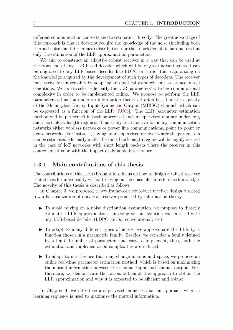
We aim to construct an adaptive robust receiver in a way that can be used atthe front end of any LLR-based decoder which will be of great advantage as it canbe migrated to any LLR-based decoder like LDPC or turbo, thus capitalizing onthe knowledge acquired by the development of such types of decoders. The receivermust strive for universality by adapting automatically and without assistance in realconditions. We aim to select efficiently the LLR parameters’ with low computationalcomplexity in order to be implemented online. We propose to perform the LLRparameter estimation under an information theory criterion based on the capacityof the Memoryless Binary Input Symmetric Output (MBISO) channel, which canbe expressed as a function of the LLR [RU08]. The LLR parameter estimationmethod will be performed in both supervised and unsupervised manner under longand short block length regimes. This study is attractive for many communicationnetworks either wireless networks or power line communications, point to point ordense networks. For instance, having an unsupervised receiver where the parameterscan be estimated efficiently under the short block length regime will be highly desiredin the case of IoT networks with short length packets where the receiver in thiscontext must cope with the impact of dynamic interference.
1.3.1 Main contributions of this thesis
The contributions of this thesis brought into focus on how to design a robust receiverthat strives for universality without relying on the noise plus interference knowledge.The novelty of this thesis is described as follows
In Chapter 3, we proposed a new framework for robust receiver design directedtowards a realization of universal receiver promised by information theory.
I To avoid relying on a noise distribution assumption, we propose to directlyestimate a LLR approximation. In doing so, our solution can be used withany LLR-based decoder (LDPC, turbo, convolutional, etc).
I To adapt to many different types of noises, we approximate the LLR by afunction chosen in a parametric family. Besides, we consider a family definedby a limited number of parameters and easy to implement, thus, both theestimation and implementation complexities are reduced.
I To adapt to interference that may change in time and space, we propose anonline real-time parameter estimation method, which is based on maximizingthe mutual information between the channel input and channel output. Fur-thermore, we demonstrate the rationale behind this approach to obtain theLLR approximation and why it is expected to be efficient and robust.
In Chapter 4, we introduce a supervised online estimation approach where alearning sequence is used to maximize the mutual information.

1.3. Aims, objectives and contributions 6
I To assess the optimal performance that can be achieved using the supervisedframework we studied it first under the long blocklength regime, we show anindirect relation between the optimization problem and minimizing the biterror rate.
I We study the robustness of the supervised approach under different noise mod-els. It is shown to be efficient for a large variety of noise distribution. Further-more, there is no need for a detection step to distinguish between Gaussianand impulsive situations.
I We propose a new LLR approximation that requires the estimation of three pa-rameters. Numerical simulations show that the performance achieved matchesthe one obtained with the true LLR and outperforms the one obtained withpreviously proposed solutions.
I We propose to evaluate the quality of the approximation by a mean squared er-ror and ascertain that this criterion is sufficient to identify the approximationsthat will be efficient instead of using the extensive Monte Carlo simulations.
I We study the effect of shortening the learning sequence and introduce themismatch risk, meaning that the learning sequence may not match the realcondition of the message.
In Chapter 5 we introduce an unsupervised online real-time estimation. It avoidsthe need of training data that reduces the useful information rate. It also allowstaking benefit from the whole data sequence to improve the accuracy of the estima-tion.
I We study the robustness of the unsupervised approach under a long block-length regime for different noise models, it exhibits a near-optimal performancein a large variety of noises and it is even better than the supervised approachif the training sequence is not sufficiently long.
I We investigate the impact of reducing the length of the packet on the BitError Rate (BER) when the LLR approximation parameters’ estimation isunsupervised.
I We analyze the reasons for the degradation that we observed compared to alonger packet case and derive an analytical tool to assess the risk of estimationfailure.
I We propose solutions to keep a robust scheme with shorter packets by increas-ing the diversity in the noise sequence extracted from the received packet andadding a regularization term.
Chapter 2Theoretical background
With the denser deployment of wireless networks, the induced interference becomesthe main system performance limitation, due to the collection of undesired signalsbroadcasted by other transmitters. If the thermal noise caused by receiver equipmentis well modeled by Gaussian distribution, it has been shown in many works thatinterference exhibits an impulsive behavior [PW10a, GCA+10, SAC04, ECdF+17] asit does not represent the impulsive nature of the interference. In this context, othermodels must therefore be considered. The study of such models is important fortwo major reasons. First, from a fundamental point of view, it brings a betterunderstanding of the phenomena. Then, from a practical point of view, it guides thedesign of communication systems and the choice of communication strategies. Thischapter presents noise/interference models often seen in the literature and introducesthe dynamic interference characterization. In particular, α-stable model and itsproperties are studied as well as their interests to model impulsive processes. This isfollowed by LDPC codes review which will be considered in the rest of this manuscriptand a brief of some useful information theory elements.
2.1 Impulsive interference
With the denser deployment of wireless networks, the induced noise and interfer-ence becomes the main system performance’s limitation on capacity, coverage,
etc. By definition, noise is an unsought signal that implicates unpredictable pertur-bations that degrade the desired information. Its source can be separated in manycategories [Vas00], for instance, acoustic noise, electronic noise, electrostatic noise,quantization noise, and communication channel, etc. Interference represents thecollection of undesired signals broadcasted by other transmitters and added to thedesired one. It is created when multiple uncoordinated links share a common com-munication medium, hence, it is featured as being a special case of artificial noisegenerated by other signals. In the cellular communication context, the frequencyplanning is used in the sake of improving the spectral efficiency and the systemcapacity, however, it will induce inevitable interference.
Limiting the impact of interference either by avoiding it or by mitigating it[CAG08, Gol05, CLCC11] is tackled in several works, in the sake of improving the
2.1. Impulsive interference 8
Fig. 2.1. Character of Impulse noise.
system capacity, the node coverage in heterogeneous networks, or any other fea-tures in the interest of system designer. Several techniques are proposed to reducethe effect of interference: interference alignment at the physical layer [EPH13], suc-cessive interference cancellation [WAYd07, And05], carrier sensing and many otheruseful techniques at the MAC layer [YV05,JHMB05] that try to avoid simultaneoustransmissions, attributing orthogonal resource blocks to different users. However,orthogonal schemes imply coordination in the network, which is not always feasible.For this reason, several techniques have been proposed as utilizing the same time-frequency resource or spatial separation [CBV+09] or the Non-Orthogonal MultipleAccess (NOMA) technique.
Creating systems with no interference is an optimal strategy, but in fact, theindispensable increase of transmitting devices may burden such an approach. An-other approach can be achieved by designing codes that benefit from the interfer-ence. This motivates the researchers to understand the fundamental characteristicsin transmissions containing interference.
Understanding the main characteristics of the noise and interference is essentialto evaluate its effect on transmission systems. A Gaussian random variable (r.v.)choice is a fundamental model justified by the Central Limit Theorem (CLT). Thismodel is attractive due to the stability property and its simplicity and its analyticaltractability. Furthermore, the optimal receiver is linear and easy to implement. Nev-ertheless, it has been shown in many works that interference exhibits an impulsivebehavior [PW10a, GCA+10, SAC04]. The receiver based on the Gaussian assump-tion exhibit a dramatic performance degradation [PW10a] in such cases. During thelast years, many new models have been investigated in various scenarios to handlethe interference phenomenon.
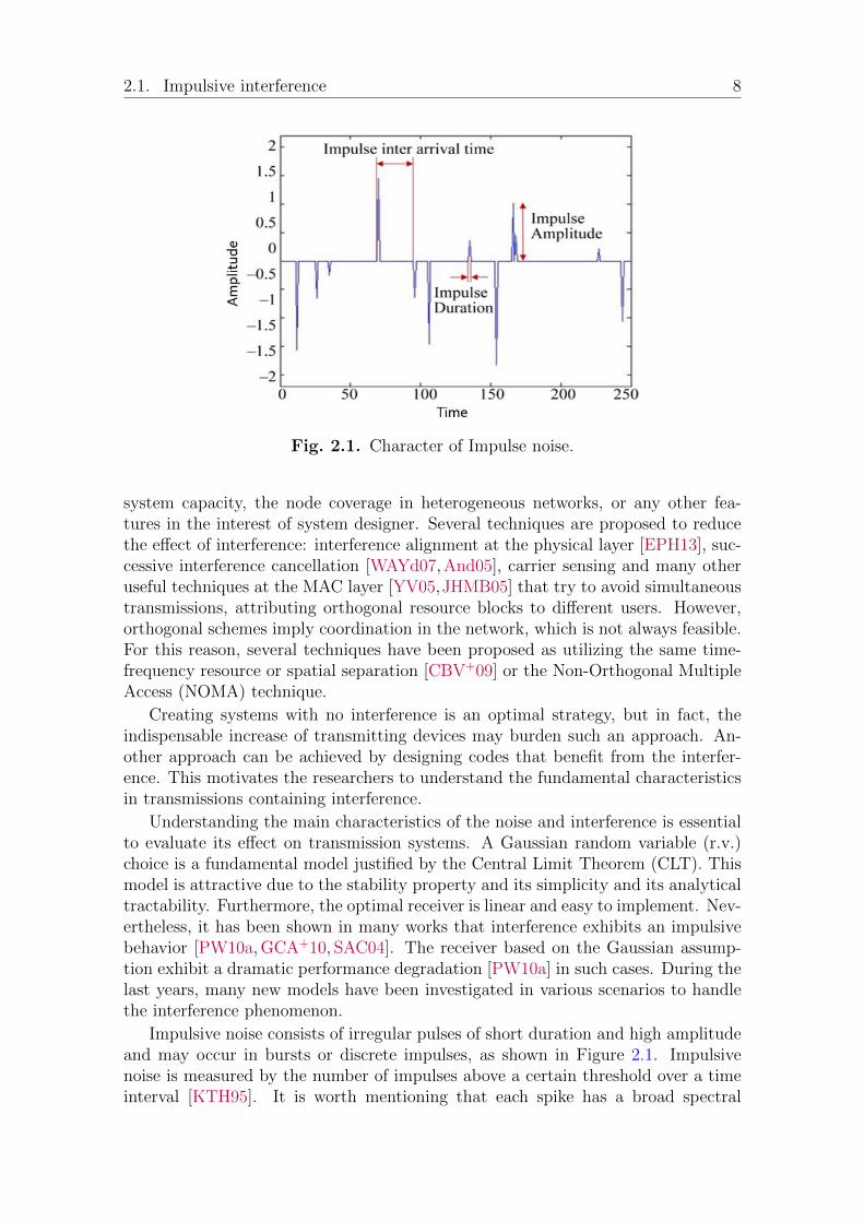
Impulsive noise consists of irregular pulses of short duration and high amplitudeand may occur in bursts or discrete impulses, as shown in Figure 2.1. Impulsivenoise is measured by the number of impulses above a certain threshold over a timeinterval [KTH95]. It is worth mentioning that each spike has a broad spectral

9 CHAPTER 2. THEORETICAL BACKGROUND
Fig. 2.2. Time and frequency sketches of (a) ideal impulse, (b) and (c) two differentshort duration pulses.
Fig. 2.3. Illustration of variation of the impulse response of a non-linear systemwith increasing amplitude of the impulse.
content. Figure 2.2 shows two examples of short-duration pulses with their respectivespectra, where m indicates the discrete-time index and f indicates the frequency. Ina communication system, at a certain point in space and time the impulsive noisewill be generated, and then propagates to the receiver through the channel.
The channel will shape the received noise which can be seen as the channel im-pulse response. Generally, the communication channel characteristics may be vari-ant or invariant, linear or non-linear. Moreover, the response to a large-amplitudeimpulse in many communication systems will exhibit a nonlinear characteristic asshown in Figure 2.3. This gives a glance behind the effect of large amplitude impulsesfrom a signal processing aspects and allows better understanding. One can definethe impulsive behavior as a random variable having a heavy-tailed probability den-sity function (PDF). From a probability theory aspect, heavy-tailed distributionsare probability distributions whose tails are not exponentially bounded, in otherwords, they have heavier tails compared to exponential distributions.
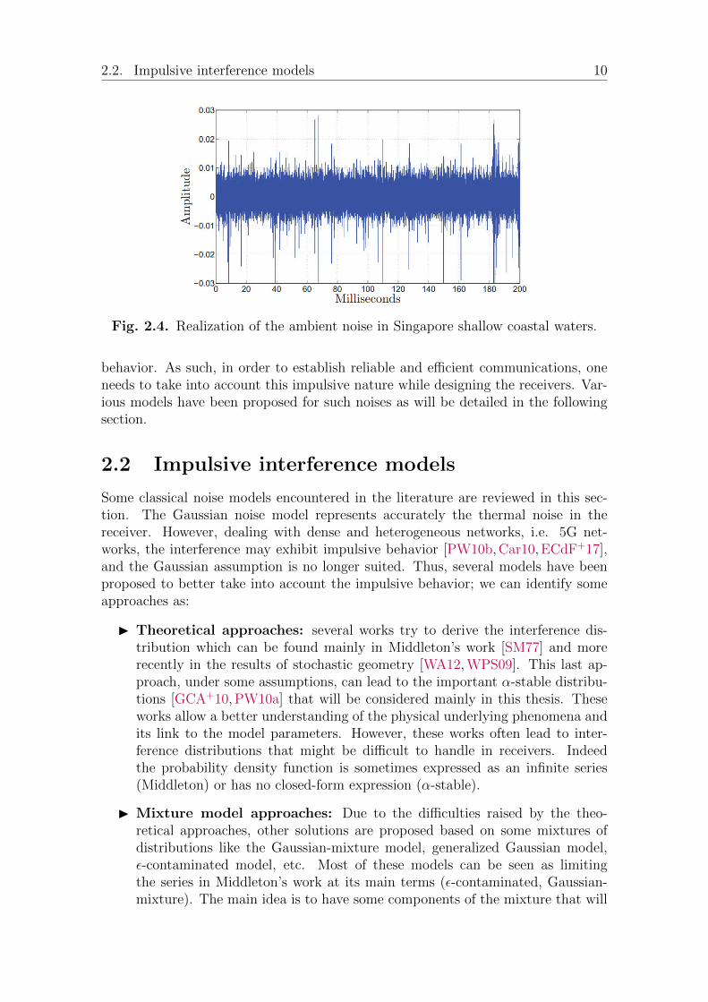
In Figure 2.4 we show the ambient noise detected by an underwater acousticreceiver operating in shallow waters of the coast of Singapore. The collected datawas taken from the National University of Singapore [KTMP03] during sea-trials bythe Acoustic Research Laboratory. Obviously, the ambient noise exhibits impulsive
2.2. Impulsive interference models 10
Fig. 2.4. Realization of the ambient noise in Singapore shallow coastal waters.
behavior. As such, in order to establish reliable and efficient communications, oneneeds to take into account this impulsive nature while designing the receivers. Var-ious models have been proposed for such noises as will be detailed in the followingsection.
2.2 Impulsive interference models
Some classical noise models encountered in the literature are reviewed in this sec-tion. The Gaussian noise model represents accurately the thermal noise in thereceiver. However, dealing with dense and heterogeneous networks, i.e. 5G net-works, the interference may exhibit impulsive behavior [PW10b, Car10, ECdF+17],and the Gaussian assumption is no longer suited. Thus, several models have beenproposed to better take into account the impulsive behavior; we can identify someapproaches as:
I Theoretical approaches: several works try to derive the interference dis-tribution which can be found mainly in Middleton’s work [SM77] and morerecently in the results of stochastic geometry [WA12, WPS09]. This last ap-proach, under some assumptions, can lead to the important α-stable distribu-tions [GCA+10, PW10a] that will be considered mainly in this thesis. Theseworks allow a better understanding of the physical underlying phenomena andits link to the model parameters. However, these works often lead to inter-ference distributions that might be difficult to handle in receivers. Indeedthe probability density function is sometimes expressed as an infinite series(Middleton) or has no closed-form expression (α-stable).
I Mixture model approaches: Due to the difficulties raised by the theo-retical approaches, other solutions are proposed based on some mixtures ofdistributions like the Gaussian-mixture model, generalized Gaussian model,ε-contaminated model, etc. Most of these models can be seen as limitingthe series in Middleton’s work at its main terms (ε-contaminated, Gaussian-mixture). The main idea is to have some components of the mixture that will

11 CHAPTER 2. THEORETICAL BACKGROUND
increase the heaviness of the tails. Mixture models may have good attributes,mainly the closed-form PDF and the existence of the 1st and 2nd order mo-ments. However, they may not truly portray the noise characteristic at thetails [Leg09] and lack the stability property, thus, restricting arguments mustbe considered in order to characterize the resulting distribution.
I Empirical approaches: they are often based on practical choices of a distri-bution that allow a good fit with generally simulated data, for instance, Paretomodel [K60], T-student model [Hal66], etc.
One can note that the aforementioned models cover the main solutions and are notan extensive list of the different impulsive models. In the following of this section,we will detail some of the most commonly used models.
2.2.1 Gaussian
The Gaussian distribution is the most common noise model used in wireless systems[Vas06,BSE10], it is characterized by two parameters: the mean µ and the varianceσ2. Essentially, it appears from external environment sources and the vibration ofatoms in conductors, known as the thermal noise. An important theorem, oftenjustifying the good adequacy of this model, is the CLT [Fel70, Dur10]: the noise isobtained by the superposition of a large number of independent contributions. Andby the CLT given below tends to be Gaussian.
Theorem 1. (Classical CLT) Let X1, X2, ..., XN be a sequence of random vari-ables independently and identically distributed (i.i.d) and let the mean µ = E [X1]and finite variance σ2 = E [(X1 − µ)2] <∞, then
1
σ√n
(n∑j=1
Xj − nµ
)d−−−→
n→∞Z ∼ N (0, 1), (2.1)
To match the following notation, this can be rewritten as
an(X1 + . . .+Xn)− bnd−−−→
n→∞Z ∼ N (0, 1), (2.2)
where an = 1/(σ√n) and bn =
√nµ/σ.
Conceptually, the CLT explains the Gaussian nature of the processes that aregenerated by the superposition of a very large number of small independent randomcauses and which present identical probability distributions. For instance, this isthe case of the thermal noise, which is generated by the superposition of a largenumber of independent random interactions at the molecular level. In summary,the CLT imposes that regardless of the Xj distribution, as n → ∞ the sum tendsto a Gaussian random variable if Xj are i.i.d. and have a finite variance.
Formally, for a continuous Gaussian random variable X the Gaussian noise PDFis given by
fG(x) =1
σ√
2πe−
(x−µ)2
2σ2 , (2.3)

2.2. Impulsive interference models 12
where µ is the mean and σ is the standard deviation. On the other hand, thecharacteristic function is represented by
φG(θ) = eiµθe−12
(σθ)2 . (2.4)
The analytical and tractable forms of the Gaussian model make it a convenientmodel. Indeed, this model appears as a universal model because of adapting tomany situations. Most of the conventional signal processing researches use thismodel. Among these situations, we find the field of communication theory wheremany algorithms assume that the studied signals obey a Gaussian law or add toGaussian noise. This hypothesis generally makes it possible to obtain compact andfast analytical solutions, but it is restrictive.
One limitation is that it is difficult to take into account a large variability in thedata. This is due to the fast tail decay of the PDF that can be quantified as
Proposition 1. Let X ∼ N (µ, σ2) then
Pr(|X − µ|> t) ≤√
2
π
σ
te−
t2
2σ2 , t > 0, (2.5)
meaning that the probability of large samples decays exponentially. As such, theprobability of having large values that appear in the interference depicted by samplesfar from the mean µ are not predicted by the Gaussian model. However, in the field oftelecommunications, many phenomena encountered have this important variabilityimpulsive by nature. Examples include noises encountered during transmission onthe power grid [ZD02], digital subscriber lines [Coo93], UWB systems [PCG+06],interference in ad hoc networks [IH98a], interference in wireless multi-user systems[Sou92a], etc.
In the following, we illustrate main approaches that have lead to impulsive mod-els: analytical approaches, for instance, Middleton class A, B, C models or undersome assumptions α-stable model and other empirical approaches based on Gaussianmixtures or mixture of distributions.
2.2.2 Middleton model
One of the first significant models in communication can be seen in Middleton’swork who described the phenomenon of impulsive noise [Mid96], where he gave amodel for impulsive noise in communications systems.
The nature, the origins, the measurement, and the prediction of the general elec-tromagnetic (EM) interference environment are a major concern of any adequatespectral management program. Middleton divided the origin of impulse noise intwo main categories: (1) man-made, which is caused by other devices connected ina communications network and (2) naturally occurring, for instance, due to thun-derstorms, and atmospheric phenomena, etc. Nevertheless, most man-made andnatural electromagnetic interference are highly non-Gaussian random processes.
General EM noise environments can be conveniently classified into three broadcategories vis-a-vis any narrow-band receiver [Mid77]: Middleton class A, class B,and class C.

13 CHAPTER 2. THEORETICAL BACKGROUND
I Class A interference (represents narrowband noise:) originally defined sothat the bandwidth of the noise is comparable to, or less than, the bandwidth ofthe receiving system [Mid72b], now modified to include all noise pulses that donot produce transients in the front end of the receiver [Mid72a]. In particular,class A noise describes the type of electromagnetic interference (EMI) oftenencountered in telecommunication applications, where this ambient noise islargely due to other, “intelligent”1 telecommunication operations.
I Class B interference (represents broadband noise:) the bandwidth of thenoise is greater than the bandwidth of the receiving system, i.e., the noisepulses produce transients in the receiver. So that transient effects, both in thebuild-up and decay, occur, with the latter predominating. Usually, ambientClass B noise represents man-made or natural “non intelligent”2 and is highlyimpulsive.
I Class C interference: a combination of Class A and Class B.
Spaulding and Middleton have studied optimum reception of signals in Class Aand B noise [SM77,Spa81].
Middleton Class A noise model is one of the most famous models which hasbeen extensively studied and utilized in the literature to become widely acceptedto model the effects of impulse noise in communications systems. Moreover, it hasbeen shown that Class A noise accurately model electromagnetic interference (EMI)and background noise, for instance, in Power line Communications (PLC) [AP10],Orthogonal Frequency-Division Multiplexing (OFDM) [III07] and Multiple InputMultiple Output (MIMO) [CGE+09].
Due to its success, we will use this model to evaluate our proposals so that wededicate space in the following to describe the Class A noise model. The PDF ofMiddleton Class A model is a Gaussian Mixture Model (GMM) with an infinitenumber of components
fM(nk) =∞∑m=0
PmN (nk; 0;σ2m), (2.6)
where N (xk;µ;σ2m) represents a Gaussian PDF with mean µ and variance σ2, and
Pm =Ame−A
m!; (2.7)
σ2m = σ2
mA
+ Γ
1 + Γ= σ2
I
m
A+ σ2
G = σ2G
( mAΓ
+ 1). (2.8)
The noise variance is σ2 which can be decomposed into two parts, σ2 = σ2G +σ2
I ,where σ2
G is the thermal noise power and σ2I is the impulsive noise power. The
1Intelligent noise or interference [Mid72b]: is man-made and intended to convey a message orinformation of some sort;
2Non-Intelligent noise or interference [Mid72b]: may be attributable to natural phenomena, e.g.,receiver noise or atmospheric noise, for example, or may be man-made, but conveys no intendedcommunication, such as automobile ignition, or radiation from power lines, etc.

2.2. Impulsive interference models 14
Fig. 2.5. Example of Impulsive index: (a) Impulsive index (density) of η impulses,each with width (duration) τ , occupying a given time period T0 and (b) impulsiveindex (density) of 3 impulses, each with width (duration) τ , occupying a given timeperiod T0 = 1.
parameter Γ = σ2G/σ
2I is the ratio between them, which gives the Gaussian to impulse
noise power. The parameter A denotes the impulsive index or more recently it isdenoted as the overlap index and used to control the impulsiveness as A > 0. Itis related to the average number of emission ”events” that collide at the receivertimes the mean duration of a typical interfering source emission [Mid77]. In otherwords, it represents the density of impulses (of a certain width) in an observationperiod. Therefore, A = ητ/T0, where η is the average number of impulses per secondand T0 = 1, which is unit time. The parameter τ , is the average duration of eachimpulse, where all impulses are taken to have the same duration. Therefore, insteadof talking about the number of impulses we use the density of impulses as shown in(2.7) where we have the density of impulse noise occurring according to a Poissondistribution.
The impulsive index A is rarely well explained in the literature, so we will givesome details to enhance its understanding. First note that A ≤ 1, this follows fromthe definition of the impulsive index being a fraction of impulses in a given periodT0. Therefore, for ητ > T0, no matter how large ητ is in the observation periodT0, the impulsive index is capped at 1. Moreover, no matter if the impulses occurwhether in bursts (next to each other) or not, the calculation of the impulsive indexfollows the same procedure. To clarify that we show in Figure 2.5 both scenarios. InFigure 2.5 (a) we present η impulses each of duration τ that occur next to each otherwhich is defined as bursts. On the other hand, in Figure 2.5 (b) we present η = 3impulses that do not necessarily occur in bursts each of duration τ , we show the

15 CHAPTER 2. THEORETICAL BACKGROUND
Fig. 2.6. PDF comparison of Middleton Class A noise with different impulsiveindex A, different Gaussian to impulsive noise power ratio Γ and compared to thenormal PDF with σ2
G = 1.
Fig. 2.7. Samples generated from a Middleton class A noise with different A, Γand σ2
G = 1.
2.2. Impulsive interference models 16
Fig. 2.8. Probability density of a Generalized Gaussian distribution with differentβ values.
usual case, in the sense that impulsive noise is sporadic by nature, the calculation ofA where spread over an observation period T0 = 1. Eventually, one can note fromFigure 2.5 that whether the impulses occur in bursts or not, the impulsive indexcalculation follows the same procedure.
Figure 2.6 compares the PDF of the Middleton Class A with different parameters’to the Normal PDF. The y-axis is given in logarithmic scale to highlight the heavinessof the tail distribution as a function of parameters. The smaller values of A produceimpulses with high amplitude samples noise as the tail of the distribution becomesheavier, thus, the probability to have severe impulses increases. Remark that despitethe fact that A = 0 degenerates into purely Gaussian (see (2.6)), conversely, as Aincreases the noise tends towards the Gaussian noise.
In Figure 2.7 we generate 2000 samples from a Middleton Class A noise withdifferent values of A and Γ. Figure 2.7 show that as A decreases (except for thespecial case A = 0) the probability to receive extremely large values will increase,however, as Γ increases the Gaussian noise will become dominant compared to theimpulsive one.
2.2.3 Generalized Gaussian distribution
The generalized Gaussian distribution (GGD) distribution has been used in severalareas such as multiple access interference in UWB systems [BY09], ad hoc networks[HEg07], in multi-user systems [ZB02], etc. This distribution is described in several

17 CHAPTER 2. THEORETICAL BACKGROUND
Fig. 2.9. Probability density of a Gaussian mixture distribution
forms [VA89], but we will use the following PDF form
f(x) =β
2αΓ(1/β)exp
(−∣∣∣∣x− µα
∣∣∣∣β)
(2.9)
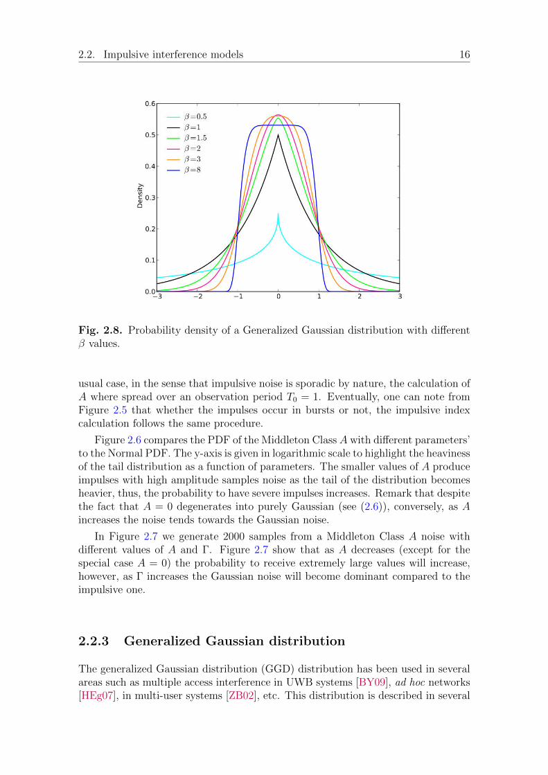
where µ ∈ R represents the location parameter, β ∈ R+ is the shape parameteror characteristic exponent, α ∈ R+ is a scaling parameter and Γ(·) is the Gammafunction. This family includes different types of distributions: Gaussian (β = 2),Laplace (β = 1) and uniform law (β →∞) as shown in Figure 2.8.
One can note that the nature of this distribution depends essentially on thevalue of the characteristic exponent β. They allow either heavier (β < 2) or lighter(β > 2) tails compared to the Gaussian case. Due to this flexibility, they becomevery useful to model the impulsive noise, however, they remain empirical withoutany theoretical justifications. In addition, when β < 1, this distribution inherits thepointed shape or peaky shape of the Laplace distribution. Furthermore, when β > 1the tails of the generalized Gaussian distributions are characterized by exponentialdecay, in contrast to the heavy tails that appear in practice [NS95,WTS88].
2.2.4 Gaussian mixture model
The Gaussian mixture [MT76,Kas88] is a statistical model represented by a densityof probability seen as a weighted combination of several weighted Gaussian. We canwrite it as follows:
f(x) =K∑k=1
λkN (x|µk, σk), (2.10)
where N (x|µk, σk) is a Gaussian density described by a vector of averages µk and avariance σk and the weighting is given by the coefficient λk that satisfies
∑Kk=1 λk =
2.2. Impulsive interference models 18
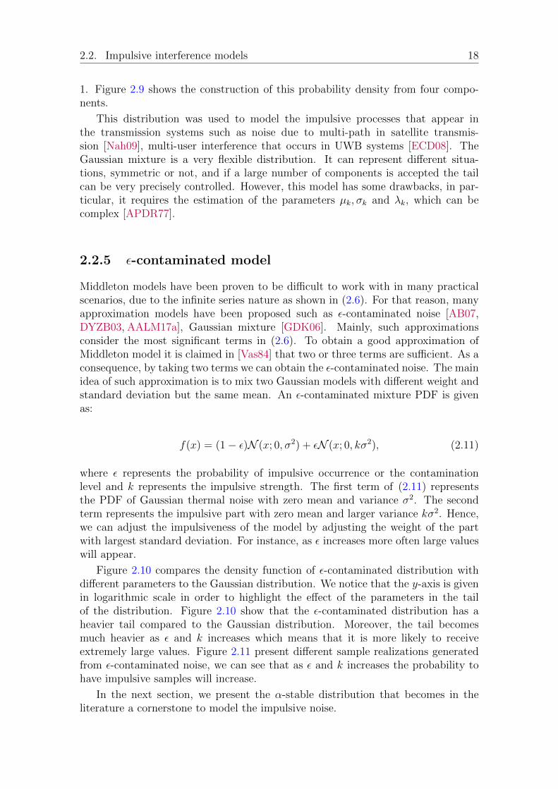
1. Figure 2.9 shows the construction of this probability density from four compo-nents.
This distribution was used to model the impulsive processes that appear inthe transmission systems such as noise due to multi-path in satellite transmis-sion [Nah09], multi-user interference that occurs in UWB systems [ECD08]. TheGaussian mixture is a very flexible distribution. It can represent different situa-tions, symmetric or not, and if a large number of components is accepted the tailcan be very precisely controlled. However, this model has some drawbacks, in par-ticular, it requires the estimation of the parameters µk, σk and λk, which can becomplex [APDR77].
2.2.5 ε-contaminated model
Middleton models have been proven to be difficult to work with in many practicalscenarios, due to the infinite series nature as shown in (2.6). For that reason, manyapproximation models have been proposed such as ε-contaminated noise [AB07,DYZB03, AALM17a], Gaussian mixture [GDK06]. Mainly, such approximationsconsider the most significant terms in (2.6). To obtain a good approximation ofMiddleton model it is claimed in [Vas84] that two or three terms are sufficient. As aconsequence, by taking two terms we can obtain the ε-contaminated noise. The mainidea of such approximation is to mix two Gaussian models with different weight andstandard deviation but the same mean. An ε-contaminated mixture PDF is givenas:
f(x) = (1− ε)N (x; 0, σ2) + εN (x; 0, kσ2), (2.11)
where ε represents the probability of impulsive occurrence or the contaminationlevel and k represents the impulsive strength. The first term of (2.11) representsthe PDF of Gaussian thermal noise with zero mean and variance σ2. The secondterm represents the impulsive part with zero mean and larger variance kσ2. Hence,we can adjust the impulsiveness of the model by adjusting the weight of the partwith largest standard deviation. For instance, as ε increases more often large valueswill appear.
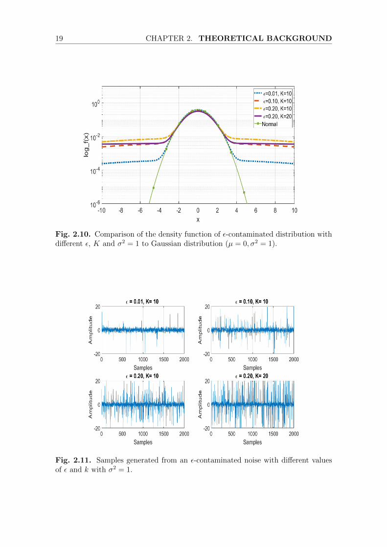
Figure 2.10 compares the density function of ε-contaminated distribution withdifferent parameters to the Gaussian distribution. We notice that the y-axis is givenin logarithmic scale in order to highlight the effect of the parameters in the tailof the distribution. Figure 2.10 show that the ε-contaminated distribution has aheavier tail compared to the Gaussian distribution. Moreover, the tail becomesmuch heavier as ε and k increases which means that it is more likely to receiveextremely large values. Figure 2.11 present different sample realizations generatedfrom ε-contaminated noise, we can see that as ε and k increases the probability tohave impulsive samples will increase.
In the next section, we present the α-stable distribution that becomes in theliterature a cornerstone to model the impulsive noise.
19 CHAPTER 2. THEORETICAL BACKGROUND
Fig. 2.10. Comparison of the density function of ε-contaminated distribution withdifferent ε, K and σ2 = 1 to Gaussian distribution (µ = 0, σ2 = 1).
Fig. 2.11. Samples generated from an ε-contaminated noise with different valuesof ε and k with σ2 = 1.

2.2. Impulsive interference models 20
2.2.6 α-stable distributions
Stable distributions also called α-stable distributions, were introduced by Paul Levyin the 1920’s. They form a very rich class of probability distributions capable ofrepresenting skewness, heavy tails and have many fascinating mathematical prop-erties. As a consequence, they are considered to be an important class that modelsimpulsive noise.
This family distribution is used in many areas such as telecommunications [CTB98],finance [BEK98], computer science [KH01], biomedical... Several books are avail-able devoted to them: Zolotarev [Zol86] studied the α-stable laws in the uni-variedcontext; Samorodnitsky and Taqqu [ST94] have studied in depth several propertiesof these laws in the univariate case as well as the multivariate case. Nikias andShao [NS95] applied these laws in the signal processing, such as signal detection andclassification, development of optimal and sub-optimal receivers in the presence ofimpulsive signals and the estimation of the parameters of an α-stable distribution.
One may adopt the α-stable distributions to describe a system essentially forthree reasons:
I The existence of theoretical justifications for the adequacy of this model.The recent work by Pinto and Win [PW10a, PW10b] are a good illustra-tion of these justifications, moreover, there are so many in the literatureNolan [Nol97, Sou92b, NS95, ST94]. One can note that, when the radius ofthe network is large with no guard zones and the active interferer set changesrapidly, the induced true interference can efficiently be approximated by stabledistributions [GEAT10, IH98b].
I The Generalized Central limit Theorem (GCLT) which states that the onlypossible non-trivial limit of normalized sums of i.i.d terms (with or withoutfinite variance) is stable. It is argued that a stable model should be used todescribe systems from which the observed quantities are results from the sumof many small terms (i.e. the noise in a communication system, the price ofstock, ..., etc).
I The third argument to adopt the stable models is empirical: many large datasets exhibit skewness and heavy tails, combining these features with the GCLTis used by many in the literature to justify the use of stable models. Examplesin communication systems which are our concern can be seen by Stuck andKleiner [SK74], Zolotarev [Zol86], Nikias and Shao [NS95]. Using a Gaussianmodel, such data sets are poorly described, however, using a stable distributionthey can be well described.
The major drawback and challenges to the use of stable distributions is thelack of closed formulas for the densities and distribution functions except for fewstable distributions such as Gaussian, Cauchy, Levy. However, reliable computerprograms nowadays allow us to compute densities numerically, distribution functionsand quantiles. With such programs, a variety of practical problems can be solvedusing stable models.
21 CHAPTER 2. THEORETICAL BACKGROUND
α-stable definitions and properties
One main property of a normal random variable is that the sum of two of them willlead to a normal random variable. Consequently, if X is normal, then for X1 andX2 independent copies of it and any a, b ∈ R>0,
aX1 + bX2d= cX + d, (2.12)
holds for some positive c ∈ R>0 and a real number d ∈ R. The symbold= means
that both right and left expressions have the same probability law (equality indistribution).
Similarly stable random variables are defined
Definition 1. A stable random variable X is said to have a stable distribution orit follows a stable law if for X1 and X2 independent copies of X all positive realnumbers a, b ∈ R>0, (2.12) holds for some positive c ∈ R>0 and a real numberd ∈ R. Particularly, if (2.12) holds with d = 0 for all choices of a and b then X is
strictly stable. If X is stable and symmetrically distributed around 0, e.g. Xd= −X
then it is symmetric stable.
One can note that the term stable is used because the shape is stable or preservedup to potential shift and scaling under sums of the type (2.12). In fact, there areother equivalent definitions of stable random variables. We will state two of themin the following.
Definition 1 can be extended to a sum of n random variables.
Definition 2. A non-degenerate Z is stable iff X1, . . . , Xn are i.i.d copies of Z andthere exist constants cn > 0 and dn ∈ R such that
X1 + . . .+Xnd= cnZ + dn. (2.13)
Lemma 1. In [P.N18, Section 3.1] it is shown that Definition 2 holds only if thescaling constants is cn = n1/α for some α ∈ (0, 2].
Putting it differently will state what is called the Generalized Central LimitTheorem.
Theorem 2. Generalized Central Limit Theorem (GCLT) for some 0 <α ≤ 2, a nondegenerate random variable Z is stable iff there is an i.i.d sequenceXii∈N, and constants cn > 0 and dn ∈ R such that
1
cn
(n∑i=1
Xi − dn
)d−−−→
n→∞Z (2.14)
or, equivalently,
limn→∞
Pr
1
cn
(n∑i=1
Xi − dn
)< x
= G(x) (2.15)
where for all continuity points x of G, G(x) denotes a non-degenerate random vari-able Z, in other words, a limiting distribution [Nol97].

2.2. Impulsive interference models 22
Theorem 2 says that the only possible non-degenerate distributions with a do-main of attraction are stable. In other words, this theorem states that if the nor-malized sum of i.i.d. random variables with or without finite variance converge toa distribution by increasing the number of variables, the limit distribution mustbelong to the family of stable laws. In particular, having a finite variance gives theCLT and the Gaussian limit distribution.
Both Definition 1 and Definition 2 use distributional properties of X or dis-tributional characterization of GCLT. While useful, these conditions do not givea concrete way of parameterizing stable distributions. However, another way todescribe stable distributions is done with the characteristic function (CF) [CL97]φX(t) = E[eitX ] =
∫∞−∞ e
itxdF (x), where X is a random variable with a distributionF (X).
Definition 3. A random variable X is stable iff Xd= γZ + δ, where γ 6= 0, δ ∈ R
and Z is a random variable with CF
E[eitX ] =
exp(−|γt|α[1− iβ tan πα
2(sign(t))] + iδt) if α 6= 1
exp(−|γt|[1 + iβ 2π(sign(t)) log |t|] + iδt) if α = 1.
(2.16)
where 0 < α ≤ 2, −1 ≤ β ≤ 1 and sign(t) defined as
sign(t) =
1 if t > 0
0 if t = 0
−1 if t < 0.
(2.17)
When β = 0 and δ = 0, these distributions are symmetric around zero and
denoted by SαS for which Xd= −X. In that case, the CF reduced to a simpler form
φ(t) = e−|γt|α
, t ∈ R. (2.18)
Except for three different cases (Normal, Cauchy, and Levy distributions), thedensity cannot be written in closed form. In practice, this appears to doom the useof stable models.
Parameterizations of stable laws
Definition 3 introduces the four parameters α, β, γ, and δ that characterize a generalstable distribution:
I The characteristic exponent or index of stability α: it characterizes the thick-ness of the distribution tail. For instance, as α increases the probability ofobserving values far from the central position is interpreted as rare events orimpulses decreases. In the wireless context, α is directly associated with thepath loss exponent of the radio channel [RSU01a]. By letting α = 0.5, 1 and2, we obtain three special cases: Levy, Cauchy and Gaussian distributions,respectively.
23 CHAPTER 2. THEORETICAL BACKGROUND
Parameter Name Range
α characteristic exponent (0,2]β skew parameter [-1, +1]γ scale parameter (0, +∞)δ location parameter (−∞, +∞)
Table 2.1 – Parameter description for Stable Distributions
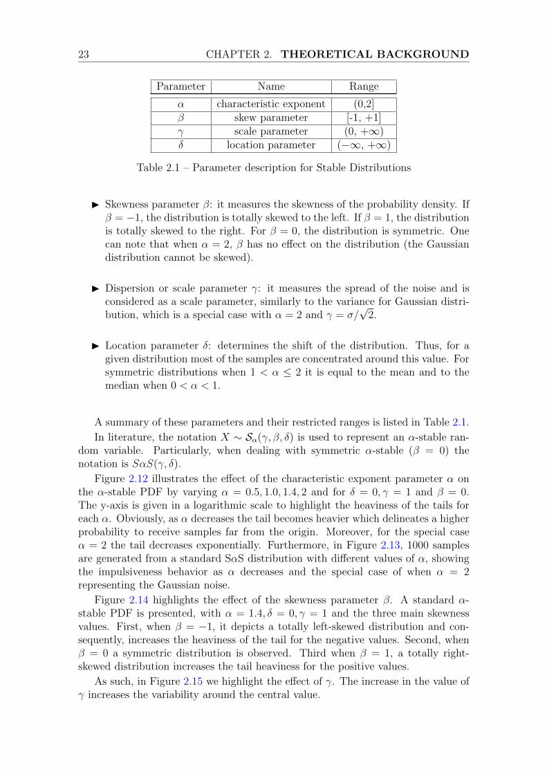
I Skewness parameter β: it measures the skewness of the probability density. Ifβ = −1, the distribution is totally skewed to the left. If β = 1, the distributionis totally skewed to the right. For β = 0, the distribution is symmetric. Onecan note that when α = 2, β has no effect on the distribution (the Gaussiandistribution cannot be skewed).
I Dispersion or scale parameter γ: it measures the spread of the noise and isconsidered as a scale parameter, similarly to the variance for Gaussian distri-bution, which is a special case with α = 2 and γ = σ/
√2.
I Location parameter δ: determines the shift of the distribution. Thus, for agiven distribution most of the samples are concentrated around this value. Forsymmetric distributions when 1 < α ≤ 2 it is equal to the mean and to themedian when 0 < α < 1.
A summary of these parameters and their restricted ranges is listed in Table 2.1.
In literature, the notation X ∼ Sα(γ, β, δ) is used to represent an α-stable ran-dom variable. Particularly, when dealing with symmetric α-stable (β = 0) thenotation is SαS(γ, δ).
Figure 2.12 illustrates the effect of the characteristic exponent parameter α onthe α-stable PDF by varying α = 0.5, 1.0, 1.4, 2 and for δ = 0, γ = 1 and β = 0.The y-axis is given in a logarithmic scale to highlight the heaviness of the tails foreach α. Obviously, as α decreases the tail becomes heavier which delineates a higherprobability to receive samples far from the origin. Moreover, for the special caseα = 2 the tail decreases exponentially. Furthermore, in Figure 2.13, 1000 samplesare generated from a standard SαS distribution with different values of α, showingthe impulsiveness behavior as α decreases and the special case of when α = 2representing the Gaussian noise.
Figure 2.14 highlights the effect of the skewness parameter β. A standard α-stable PDF is presented, with α = 1.4, δ = 0, γ = 1 and the three main skewnessvalues. First, when β = −1, it depicts a totally left-skewed distribution and con-sequently, increases the heaviness of the tail for the negative values. Second, whenβ = 0 a symmetric distribution is observed. Third when β = 1, a totally right-skewed distribution increases the tail heaviness for the positive values.
As such, in Figure 2.15 we highlight the effect of γ. The increase in the value ofγ increases the variability around the central value.

2.2. Impulsive interference models 24
Fig. 2.12. Effect of the characteristic exponent parameter α on the α-stable PDFwith δ = 0, γ = 1 and β = 0 and varying α = 0.5, 1.0, 1.4, 2.
Fig. 2.13. Effect of the characteristic exponent parameter α on the noise Samplesgenerated by an α-stable noise with δ = 0, γ = 1 and β = 0 and varying α =0.5, 1.0, 1.5, 2.

25 CHAPTER 2. THEORETICAL BACKGROUND
Fig. 2.14. Effect of the symmetry parameter β on the α-stable PDF for α =1.1, γ = 1, δ = 0 and varying the skewness β = −1, 0, 1.
Fig. 2.15. Effect of the dispersion parameter γ on the α-stable PDF for α =1.4, δ = 0, β = 0 and varying the dispersion β = 0.2, 0.4, 0.6, 0.8.
2.2. Impulsive interference models 26
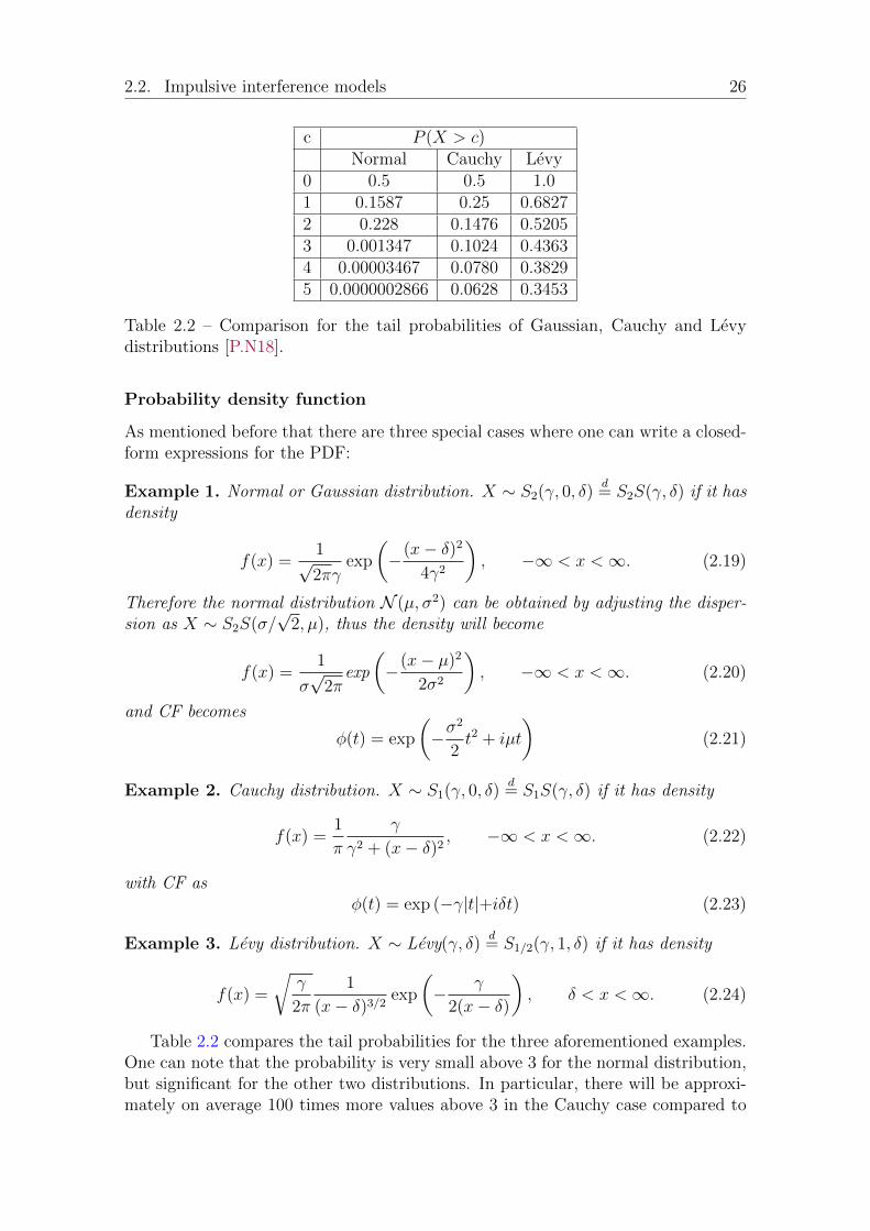
c P (X > c)Normal Cauchy Levy
0 0.5 0.5 1.01 0.1587 0.25 0.68272 0.228 0.1476 0.52053 0.001347 0.1024 0.43634 0.00003467 0.0780 0.38295 0.0000002866 0.0628 0.3453
Table 2.2 – Comparison for the tail probabilities of Gaussian, Cauchy and Levydistributions [P.N18].
Probability density function
As mentioned before that there are three special cases where one can write a closed-form expressions for the PDF:
Example 1. Normal or Gaussian distribution. X ∼ S2(γ, 0, δ)d= S2S(γ, δ) if it has
density
f(x) =1√2πγ
exp
(−(x− δ)2
4γ2
), −∞ < x <∞. (2.19)
Therefore the normal distribution N (µ, σ2) can be obtained by adjusting the disper-sion as X ∼ S2S(σ/
√2, µ), thus the density will become
f(x) =1
σ√
2πexp
(−(x− µ)2
2σ2
), −∞ < x <∞. (2.20)
and CF becomes
φ(t) = exp
(−σ
2
2t2 + iµt
)(2.21)
Example 2. Cauchy distribution. X ∼ S1(γ, 0, δ)d= S1S(γ, δ) if it has density
f(x) =1
π
γ
γ2 + (x− δ)2, −∞ < x <∞. (2.22)
with CF asφ(t) = exp (−γ|t|+iδt) (2.23)
Example 3. Levy distribution. X ∼ Levy(γ, δ)d= S1/2(γ, 1, δ) if it has density
f(x) =
√γ
2π
1
(x− δ)3/2exp
(− γ
2(x− δ)
), δ < x <∞. (2.24)
Table 2.2 compares the tail probabilities for the three aforementioned examples.One can note that the probability is very small above 3 for the normal distribution,but significant for the other two distributions. In particular, there will be approxi-mately on average 100 times more values above 3 in the Cauchy case compared to

27 CHAPTER 2. THEORETICAL BACKGROUND
the Gaussian. Which illustrates the reason behind calling the stable distributionsas heavy-tailed. Moreover, both normal and Cauchy distributions are symmetric,while the Levy distribution is totally skewed to the right with all the probabilityconcentrated on x > 0.
For α-stable random variables, there is no explicit expression of the probabilitydensity in the general case. However, we can obtain an expression in the form ofthe inverse Fourier transform of the characteristic function as
fX(x) =1
2π
∫ ∞−∞
exp(−itx)φX(t)dt. (2.25)
If X is symmetric,
fX(x) =1
2π
∫ ∞−∞
e−itxe−γα|t|αdt.
=1
π
∫ ∞0
e−γα|t|α cos(xt)dt. (2.26)
Nikias and Shao presented a simple asymptotic expansion that may well ap-proximate the probability density function fX of stable variables with unitary scaleparameter [NS95].
Proposition 2. (Asymptotic Expansion). Let X ∼ Sα(1, 0, 0), the correspond-ing probability density function fX can be approximated as
fX(x) =n∑k=1
bk|x|αk+1
+O(|x|−α(n+1)−1
), (2.27)
Corollary 1. Suppose that X ∼ Sα(1, 0, 0) with a probability density function fX(x),for x large enough, fX(x) can be written as
fX(x) ∝ |x|−(α+1) (2.28)
where (2.28) is based on the first term of (2.27) (see [NS95] for more details).
Tails and moments
The asymptotic tail properties for the normal distribution (α = 2) is well under-stood. A brief discussion is given in the following about the tails of non-Gaussian(α < 2) stable laws. When α < 1 and β = ±1, stable distributions will have onetail, while for all other cases it will have both tails, these tails are asymptoticallypower laws with heavy tails.
Proposition 3. Let X ∼ Sα(γ, β, δ) with 0 < α < 2, thenlimx→∞ x
α Pr(X > x) = γαCα1+β
2right tail,
limx→∞ xα Pr(X < −x) = γαCα
1−β2
left tail.(2.29)
where the constant Cα depends on α and is given as
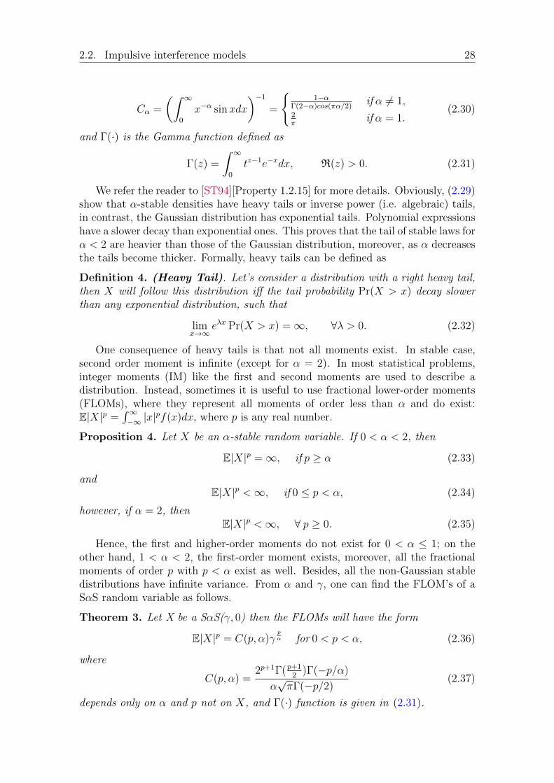
2.2. Impulsive interference models 28
Cα =
(∫ ∞0
x−α sinxdx
)−1
=
1−α
Γ(2−α)cos(πα/2)if α 6= 1,
2π
if α = 1.(2.30)
and Γ(·) is the Gamma function defined as
Γ(z) =
∫ ∞0
tz−1e−xdx, R(z) > 0. (2.31)
We refer the reader to [ST94][Property 1.2.15] for more details. Obviously, (2.29)show that α-stable densities have heavy tails or inverse power (i.e. algebraic) tails,in contrast, the Gaussian distribution has exponential tails. Polynomial expressionshave a slower decay than exponential ones. This proves that the tail of stable laws forα < 2 are heavier than those of the Gaussian distribution, moreover, as α decreasesthe tails become thicker. Formally, heavy tails can be defined as
Definition 4. (Heavy Tail). Let’s consider a distribution with a right heavy tail,then X will follow this distribution iff the tail probability Pr(X > x) decay slowerthan any exponential distribution, such that
limx→∞
eλx Pr(X > x) =∞, ∀λ > 0. (2.32)
One consequence of heavy tails is that not all moments exist. In stable case,second order moment is infinite (except for α = 2). In most statistical problems,integer moments (IM) like the first and second moments are used to describe adistribution. Instead, sometimes it is useful to use fractional lower-order moments(FLOMs), where they represent all moments of order less than α and do exist:E|X|p =
∫∞−∞ |x|
pf(x)dx, where p is any real number.
Proposition 4. Let X be an α-stable random variable. If 0 < α < 2, then
E|X|p =∞, if p ≥ α (2.33)
andE|X|p <∞, if 0 ≤ p < α, (2.34)
however, if α = 2, thenE|X|p <∞, ∀ p ≥ 0. (2.35)
Hence, the first and higher-order moments do not exist for 0 < α ≤ 1; on theother hand, 1 < α < 2, the first-order moment exists, moreover, all the fractionalmoments of order p with p < α exist as well. Besides, all the non-Gaussian stabledistributions have infinite variance. From α and γ, one can find the FLOM’s of aSαS random variable as follows.
Theorem 3. Let X be a SαS(γ, 0) then the FLOMs will have the form
E|X|p = C(p, α)γpα for 0 < p < α, (2.36)
where
C(p, α) =2p+1Γ(p+1
2)Γ(−p/α)
α√πΓ(−p/2)
(2.37)
depends only on α and p not on X, and Γ(·) function is given in (2.31).

29 CHAPTER 2. THEORETICAL BACKGROUND
Fig. 2.16. FLOM’s for a SαS random variable with different values of α.
Proof. We refer the reader to [SN93] for details.
Figure 2.16 shows the moments of order p for different α values correspondingto the (2.36) and (2.37) in Theorem 3.
Many author’s [NS95, ST94, Zol86], have investigated the fractional momentsto represent in different contexts the density of univariate and bivariate randomvariables. Indeed, they are important when the density of the random variable hasinverse power-law tails and, consequently, it lacks integer order moments. Moreover,FLOMs can be used as a measure of the dispersion of a stable distribution, and areused in some estimation schemes.
Nevertheless, FLOMs has some limitations as they do not provide a universalframework for the characterization of algebraic tail processes: when p ≥ α, the mo-ments become infinite and the statistical characterization is then no longer possible;In order to overcome this difficulty Gonzalez proposed in [GPA06, Gon97] anotherapproach based on zero order statistics (ZOS) which use logarithmic moments. Thelatter makes it possible to introduce new parameters that allow characterizing theimpulsive processes with an infinite variance which is based on so-called logarithmicprocess classes [Zol86].
Remark 1. In the case of an impulsive environment with α < 2, the second-ordermoment of a stable variable is infinite as shown before, making the conventionalnoise power measurement infinite. However, this does not mean that there are noother adequate measures of variability of stable random variables. Accordingly, in therest of this thesis, we present our simulation results as a function of the dispersionof a stable random variable γ, which is used as a measurement of the strength of theα-stable noise and plays an analogous role of the variance [BSF08, Theorem 3].

2.2. Impulsive interference models 30
Parameter estimation
The knowledge of the parameters plays a significant role in the performance of thereceiver. In the literature, several approaches exist to estimate them. Due to thelack of analytical expressions most of the methods are based on the law of largenumbers and rely on the observed samples at the receiver side. Classical parameterestimation techniques for SαS random variables can be categorized into six maincategories [WLGM15]; 1- Fractional lower order moment (FLOM) method [BMA10],2- Method of log-cumulant (MoLC) [HSSL11], 3- Extreme value method (EVM),4- Maximum likelihood (ML) [DuM73], 5- Quantile method (QM), 6- Empiricalcharacteristics function (ECF). We discuss the latter three methods.
I The maximum likelihood (ML) method: It is known that the ML ap-proach is widely favored due to its generality and asymptotic efficiency [Yu04].DuMouchel [DuM73] proposed this method and under the assumption of δ =0, β = 0 he obtained a ML estimation of α and γ. He showed that the estima-tion of the parameters is asymptotically normal and consistent after approxi-mating the likelihood function by multinomial.
I Quantiles method: Fama and Roll originate the quantile method in [FR71].They gave an approximation of the dispersion γ using the sample quantilesproperties of the SαS variable. Thereafter, they used the tail property ofthe α-stable distributions to estimate the parameter α. Later, the work ofMcCulloch [McC86a] makes the quantile method much more desired after itsextension to include asymmetric distributions and for cases where α ∈ [0.6, 2],unlike the former approach that restricts it to α ≥ 1.
I Empirical characteristic function (ECF): This method was discussed in[Yu04]. Although the likelihood function can be unbounded or not be in aclosed-form, its Fourier transform, which gives the CF hence the name of thismethod, is always bounded and has a closed form expression. The ECF realand imaginary parts will provide estimates of the parameters through givenexpressions. One can note that such a method provides an alternative way toenvision the regression estimation method.
Nolan [Nol97] provides a useful software package that can be used to estimatethe parameters of the stable distributions. Extensively, Zolotarev [Zol86] discusseda more theoretical approach to the statistical estimation of the parameters of stablelaws. Readers interested in how to simulate stable process can refer to two excellentworks of literature, Weron [WW95] and Zolotarev [Zol86].
Among the known techniques for parameter estimation, only QM, FLOM andMoLC yield to a closed form expression [WLGM15, WLF14]. However, it is worthmentioning that they are computationally expensive as they require either tablesobtained through linear interpolation as for the QM, or for ECF method one needsMonte-Carlo approach to approximate the CF. Eventually, the burden of these meth-ods is too expensive in terms of time and number of computations or under shortsequences the variances of their estimates are high. As a result, they are inconvenientfor online estimation, in other words, for applications that require low latency.

31 CHAPTER 2. THEORETICAL BACKGROUND
In this thesis, we propose a solution to design a robust receiver that does not relyon noise knowledge. Hence, it allows us to overpass the need of the noise distributionparameters estimation which is a considerable advantage. Furthermore, it shows agood performance even with a few number of samples.
Properties and further definitions
Property 1. (Stability property). let X1, X2 be independent stable r.v. withthe same characteristic exponent α as X1 ∼ Sα(γ1, β1, δ1) and X2 ∼ Sα(γ2, β2, δ2).Then, by adding the two r.v’s X3 = X1 + X2 we get a new stable r.v. X3 ∼Sα(γ3, β3, δ3) with(
γ3 = (γα1 + γα2 )1α ; β3 =
β1γα1 + β1γ
α1
γα1 + γα2; δ3 = δ1 + δ2
). (2.38)
Corollary 2. Let Xi ∼ Sα(γi, 0, 0), i = 1, 2, . . . , K, then∑K
i=1Xi ∼ Sα(γ, 0, 0)
where γ = (∑K
i=1 γαi )
1α .
Property 2. (Scaling property). Suppose X ∼ Sα(γ, β, δ), then scaling X by anon null constant b ∈ R 6=0 will give
bX ∼ Sα (|b|γ, sign(b)β, bδ) , if α 6= 1
bX ∼ S1 (|b|γ, sign(b)β, bδ − 2/πγβb(ln |b|) , if α = 1 (2.39)
Corollary 3. Suppose X ∼ Sα(γ, β, δ) where 1 < α < 2, then multiplying X by areal positive constant b ∈ R+ gives
bX ∼ Sα(bγ, β, bδ). (2.40)
The following property concerns the asymptotic behavior of the probability den-sity function of a SαS distributions as presented by Samorodnitsky and Taqqu[ST94].
Property 3. (Asymptotic behavior). Let X ∼ Sα(γ, 0, δ) then the probabilitydensity function fX(x) satisfies
fX(x) =α(1− α)γα
Γ(2− α) cos(απ2
)|x|−α−1 as |x| → ∞. (2.41)
2.3 Physical mechanism that leads to α-stable model
We claimed before that one of the main reasons to adopt the α-stable model is thetheoretical justifications behind it. In this section, we will demonstrate that an α-stable model may arise from a realistic physical mechanism under some reasonableassumptions and conditions. The transmission in a common band between networkswith different protocols, multiple applications, etc, will end up with different datatype and different symbol durations, these types of networks are known as hetero-geneous networks [AGM+15]. In particular, the network heterogeneity comes out inad-hoc networks and small-cells due to the variations in transmit power constraintsand the varied placement of the base stations.
Two key physical mechanisms can create dynamic interference:
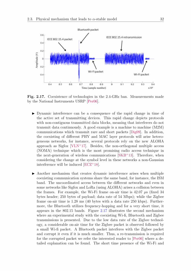
2.3. Physical mechanism that leads to α-stable model 32
Fig. 2.17. Coexistence of technologies in the 2.4-GHz ban. Measurements madeby the National Instruments USRP [Per06].
I Dynamic interference can be a consequence of the rapid change in time ofthe active set of transmitting devices. This rapid change depicts protocolswith non-contiguous transmitted data blocks, meaning that interferers do nottransmit data continuously. A good example is a machine to machine (M2M)communications which transmit rare and short packets [Dig09]. In addition,the coexisting of different PHY and MAC layer protocols will arise hetero-geneous networks, for instance, several protocols rely on the new ALOHAapproach as Sigfox [VLN+17]. Besides, the non-orthogonal multiple access(NOMA) technique which is the most promising radio access technique inthe next-generation of wireless communications [SKB+13]. Therefore, whenconsidering the change at the symbol level in these networks a non-Gaussianinterference will be induced [ECZ+18].
I Another mechanism that creates dynamic interference arises when multiplecoexisting communication systems share the same band, for instance, the ISMband. The uncoordinated access between the different networks and even insome networks like Sigfox and LoRa (using ALOHA) arises a collision betweenthe frames. For example, the Wi-Fi frame on-air time is 42.07 µs (fixed 34bytes header; 250 bytes of payload; data rate of 54 Mbps); while the Zigbeeframe on-air time is 1.28 ms (40 bytes with a data rate 250 kbps). Further-more, the Bluetooth utilizes frequency-hopping and for a very short time, itappears in the 802.15 bands. Figure 2.17 illustrates the second mechanismwhere an experimental study with the coexisting Wi-fi, Bluetooth and Zigbeetransmissions is presented. Due to the low data rate of the Zigbee technol-ogy, a considerable on-air time for the Zigbee packet is observed followed bya small Wi-fi packet. A Bluetooth packet interferes with the Zigbee packetand corrupt it even if it is much smaller. Thus, a re-transmission is requiredfor the corrupted packet we refer the interested reader to [Per06] where a de-tailed explanation can be found. The short time presence of the Wi-Fi and

33 CHAPTER 2. THEORETICAL BACKGROUND
Bluetooth interferers compared to Zigbee transmissions will result in dynamicinterference which means independent in time.
By considering a large scale wireless communication networks composed of Kaccess points and K devices, where each device transmit data to a unique accesspoint. Several works assert that the channel is characterized by a memoryless addi-tive isotropic α-stable noise (AIαSN) [PW10a,PW10b,ECdF+17].
2.4 Low-Density Parity-Check codes
The aim of channel coding is to make the noisy channel behave like a noiselesschannel. The main idea behind forward error correction (FEC) or channel codingis to increase the message length with deliberately introduced repetition, by addingextra check bits to produce a codeword for the message. In other words, the checkbits are added on purpose of having distinct codewords, thus, any corrupted bitswithin a codeword induced by noisy channel can be inferred correctly at the receiverside.
2.4.1 History and definitions
Low-Density Parity-Check (LDPC) codes first proposed in the PhD dissertationof Gallager in 1960 and then published in [Gal63] are FEC codes. LDPC codeswere mostly ignored for a long time over 35 years, due to the computational limi-tation of the hardware. More precisely, the computational demands of simulationsin an era when vacuum tubes were only just being replaced by the first transistors.Meanwhile, the development of Reed-Solomon codes in addition to highly struc-tured algebraic block and convolutional codes dominate the field of forward errorcorrection. Despite the huge practical success of these codes, their performance fellway far from the theoretical achievable limits set down by Shannon in his seminal1948 paper [Sha48]. One can note that by the late 1980s, most of the researchersresigned to this seemingly insurmountable theory, despite decades of attempts. In1981, Tanner [Tan81] proposed a graphical representation of the LDPC codes knownas Tanner graphs.
Berrou, Glavieux, and Thitimajshima transformed thoroughly the relative qui-escence of the coding field by introducing ”turbo codes” in 1993. Turbo-codes arebased on two concepts: the concatenation of two sub-codes and decoding usingfeedback. Thereafter, all the main components of successful error-correcting codeswere replaced: turbo codes focus on average rather than worst-case performance,employ iterative, distributed algorithms, rely on soft information extracted from thechannel. Using such decoders with manageable complexity, the gap to the Shannonlimit was all but eliminated. Eventually, turbo-codes paved the way for correctivecodes to approach the Shannon limit with manageable length codes and decodingthat can be implemented effectively. As researchers struggled just to understandthe successfulness of turbo codes through the 1990s, MacKay and Neal, introduceda new class of block codes in 1996 [MN96] where most of the turbo code featuresare possessed. In fact, it was recognized that such block codes are just a rediscovery

2.4. Low-Density Parity-Check codes 34
Fig. 2.18. Illustration of a parity check matrix and tanner graph representation.
of the LDPC codes developed by Gallager [Gal63]. Indeed, the decoding algorithmfor turbo codes was shown to be a special case of the decoding algorithm for LDPCcodes.
Subsequently, irregular LDPC codes were introduced which easily outperformthe best turbo codes and they can be seen as a generalization of the regular LDPCcodes. Moreover, they offer some practical advantages and a disputable cleanersetup for theoretical results. MacKay proposed Non-Binary (NB) LDPC codes overfinite fields [DM98]. It was shown that NB-LDPC codes outperform the binaryLDPC codes, but with a higher decoding complexity. Consequently, many works areproposed to reduce such complexity [GCGD07,PFD08,BD03,WSM04,DF07,Sav08].Nowadays, several design techniques for LDPC codes exist which gives the power toconstruct codes that approach within hundredths of a decibel to Shannon’s capacity[SFRU01].
In addition to the strong theoretical interest in LDPC codes, such codes arewidely used in various applications and standards due to: their superior decodingperformance [SFRU01,RSU01b]; power efficiency [MS02,PCZ+11]; high-throughputcapabilities [KC04,ZHW11]; their advantages related to hardware implementations,such as low-cost [BALE+07,DHB06]. Consequently, these codes are gradually replac-ing other well-established FEC schemes [RCS+11]. One can mention Satellite-baseddigital video broadcasting 2nd generation (DVB-S2/T2/C2), ITU-T standard fornetworking over power lines, phone lines and coaxial cable (G.hn/ G.9960), in IEEEwireless local area network standards like Wi-Fi Standard (802.11n-2009), WiMAX(802.16e), etc. Moreover, LDPC codes have been proposed as a potential candidatefor 5G cellular system [Mau16].
An LDPC code is a linear block code defined by a (M,N) sparse parity-checkmatrix denoted by H. The M rows and N columns corresponds to the parity checkequations and the coded bits, respectively. A vector v = (v1, . . . , vN) ∈ 0, 1N is acodeword iff:
HvT = 0 mod 2. (2.42)

35 CHAPTER 2. THEORETICAL BACKGROUND
By assuming a full rank matrix H and systematic code, any codeword of length Nis comprised of K = N −M information bits and M parity bits. The coding rateof the code is given by R = K/N which characterizes the amount of redundancy.Figure 2.18 depicts a miniature example of H with an illustration of its Tannergraph representation also known as a bipartite graph. It consists of two sets ofnodes: variable-nodes represent H columns (coded bits); check-nodes represent rowsof H (parity-check equations). The edges connecting both sets correspond to the1’s entries of H.
2.4.2 Construction of LDPC codes
Normally, two ways can be used to construct a LDPC code: algebraic constructionand random construction [Joh08]. The latter gives a good performance when largecode lengths LDPC codes are considered since they avoid short cycles in the Tannergraph. However such cycles are highly probable when constructing short lengthLDPC codes and for an irregular LDPC ensemble, the minimum distance becomesa critical issue as it is related to the level of error floor phenomenon. On the otherhand, a famous construction method called the Progressive Edge-Growth (PEG)algorithm was proposed in [XEA05] which can effectively construct LDPC codeswith medium or short length. PEG algorithm allows constructing the tanner graphwith a large girth by progressively establishing edges between variable and checknodes. Two main advantages result by using the PEG algorithm: first, it is veryflexible in the sense that it can be used to construct codes for any code length andcode rate, furthermore, linear time encoding is feasible under certain modifications.Second, the simplicity to construct LDPC codes with a good girth property.
2.4.3 Decoding
The majority of LDPC codes cannot be decoded algebraically due to their lengthand the limited structure of their parity matrix. Thus the decoding algorithms arebased, like turbo codes, on an iterative process. These algorithms are not optimalfor MAP decoding but allow to approach the Shannon boundary on simple channels.The non-optimality is explained by the fact that the graph representing LDPC codeshas cycles. Authors in [ETV99] show that cycle-free Tanner graphs cannot supportgood codes, moreover, the 4-cycle are inevitable for many classical binary linearblock codes as shown in [HGC06]. The minimum distance of LDPC codes that havea representation without cycles is low regardless of the performance. The use ofiterative decoding in Turbo and LDPC codes is an important element to achieve agood performance. For LDPC codes, the iterative message-passing algorithm hasshown a close performance compared to the maximum likelihood method with verylow complexity.
The advantage of LDPC codes over other codes is that they have relevant de-coding whose complexity only varies linearly with the length of the code. Thisimportant aspect is mainly due to the low density of the parity matrix. To decodeLDPC codes, a class of algorithms based on message passing along the edges ofthe tanner graph which is so-called message passing algorithms. Two types can

2.4. Low-Density Parity-Check codes 36
Fig. 2.19. Illustration of three regions characterizing the performance of an LDPCcode.
be identified by observing the messages passing through the graph: hard decisionand soft decision. The former corresponds to binary messages such as bit flippingalgorithms [Gal63] (Gallager A and B) and the latter corresponds to probabilitiesor log-likelihood ratios (LLRs) such as sum-product algorithm (SPA).
The Belief Propagation (BP) and Min-Sum algorithms are the most importantdecoding algorithms. One can note that implementing the BP algorithm is complexdue to the calculation products, and evaluating hyperbolic trigonometric functionsat the check node. Even if these functions are tabulated, the number of evaluationsremains important. At high signal-to-noise ratio, few messages are erroneous, inthis case, the magnitudes of the messages from check node to variable node arelarge and their hyperbolic tangent will be close to +1 or −1. As a result, duringthe Check-Pass only the message of lower magnitude will be taken into account inthe product and that’s where the Min-sum algorithm name came from. Hence theseremarks make it possible to greatly simplify the complexity of decoding.
Using advanced coding techniques, the evolution of the code performance infunction of the signal-to-noise ratio can be divided into three regions as shown inFigure 2.19. The first corresponds to a behaviour where the decoding does notconverge (non-convergence region), the decoding then tends to degrade performancecompared to an uncoded system. From a certain signal-to-noise ratio, called theconvergence threshold or decoding threshold, the decoding enters a phase known asthe waterfall region where the probability of error decreases very quickly with thesignal to noise ratio. Finally, the error floor region where the probability of errordecreases less rapidly than the waterfall region. The coding gain corresponds tothe difference between two systems in terms of the required energy per useful bit toachieve a given error rate.

37 CHAPTER 2. THEORETICAL BACKGROUND
2.4.4 Analyzing tools
One can mention three different techniques to analyze the iterative decoding, inparticular, the asymptotic performance of LDPC codes: Density evolution, GaussianApproximation, and EXIT charts.
I Density Evolution (DE): such a method is used to analyze the asymp-totic performance of iterative decoders [RU01]. A main objective of using DEfor LDPC codes with Message-Passing decoding is to find the SNR decodingthreshold (convergence threshold) of a specific LDPC ensemble whose lengthtends to infinity, by tracking the messages transmitting information on emit-ted codeword back and forth on the bipartite graph. Extending the DE toirregular LDPC ensembles will allow designing it by enabling optimization ofthe degree distribution [RSU01b]. Nevertheless, the large amounts of numeri-cal calculations required by the DE will arise with instability and complexity,in particular, when tracking the messages from check to variable nodes. Forsuch a reason, authors in [SFRU01] proposed the quantized density evolution(QDE) method and showed that with only 11-bit quantization one can avoidthe instability and reduce the complexity.
I Gaussian Approximation (GA): another solution to reduce the complex-ity and implement the DE was proposed in [SUR00] denoted as Gaussian ap-proximation (GA). This method was proposed for binary-input additive whiteGaussian noise (BI-AWGN) channels. The GA method assumes that the mes-sage passed through iterative decoders is Gaussian or Gaussian mixtures. Thealgorithm tracks the parameters of the message distributions instead of track-ing whole densities in the decoding process. Thus, a huge reduction in thecomplexity will be gained as one needs to track only the messages’ densitymean and variance.
I EXIT charts: the extrinsic information transfer (EXIT) chart was proposedas an alternative method compared to DE and GA. It was proposed in firstto track the exchange of intrinsic information between component decoders[ten01, Hag04]. Then it was extended to LDPC codes [tKA04] as a tool todesign good codes and to find the decoding threshold SNR by reducing it toa curve-fitting problem.
Nevertheless, the DE, GA and EXIT chart assumes that the LDPC codes areinfinite codeword length and cycle-free. Moreover, both GA and EXIT charts rely onthe assumption that the channel is Gaussian, thus, they cannot be applied directlywhen a non-Gaussian noise has to be considered. However, DE can be applied toany binary memory-less symmetric output (MBISO) channels including Gaussianand non-Gaussian i.e SαS noise.
LDPC code design is out of the scope of this thesis. Because we focus on designingan estimation of the LLR without relying on the interference plus noise knowledgesuch that it can adapt for Gaussian or impulsive noise. Thus, one can use anytype of LLR based decoders (i.e LDPC, turbo codes, ..., etc) over any Gaussian ornon-Gaussian channel type and still observe an improvement compared to the linear

2.5. Elements of Information theory 38
receiver designed only for Gaussian noise. Furthermore, having such a solution isof great advantage and it is considered inevitable when it comes to designing codesfor a specific channel because it solves the problem of mismatch decoding that hasa significant influence in the receiver performance.
2.5 Elements of Information theory
In this section, we outline the machinery to measure the information that passesthrough the channel. We introduce some notions and definitions that will be usefulin our study.
Definition 5. (Discrete channel.) A discrete channel is a statistical model withan input X and an output Y . During each signaling interval (symbol period), thechannel accepts an input symbol from X, and in response, it generates an outputsymbol from Y , generally a noisy version of X. The channel is discrete when thealphabets of X and Y are both finite.
Definition 6. (Memoryless channel.) A channel, characterized by its transitionprobability p(y|x), is said to be memoryless3 if when we transmit a sequence x =x1, x2, . . . , xN and observe a sequence of output symbols y = y1, y2, . . . , yN,
p(y|x) =N∏n=1
p(yn|xn), (2.43)
in other words, the current output symbol depends only on the current input symboland not on any of the previous input symbols which means that there is no Inter-Symbol Interference.
Definition 7. (Symmetric channel.) Assume a random variable Y that takeson a possible value in R. We say that a binary memoryless is symmetric4 (moreprecisely, output-symmetric) if
p(y|x = +1) = p(−y|x = −1), (2.44)
or as defined by Gallager (1968), if the set of outputs can be partitioned into subsetsin such a way that for each subset the matrix of transition probabilities has theproperty that each row (if more than 1) is a permutation of each other row and eachcolumn is a permutation of each other column.
Definition 8. (Ensemble X). An ensemble X is a triple (x,AX ,PX), where theoutcome x is the random variable value, which takes on one of a set possible values,AX = a1, a2, . . . , aI, having probabilities PX = p1, p2, . . . , pI, with P (x = ai) =pi, pi ≥ 0 and
∑ai∈AX P (x = ai) = 1.
3The above definition is adequate if we restrict ourselves to channels without feedback.4It is a consequence of the definition of the symmetric channel that H(Y |X) is independent of
the input distribution p(x), and depends only on the channel probabilities p(yj |xi).
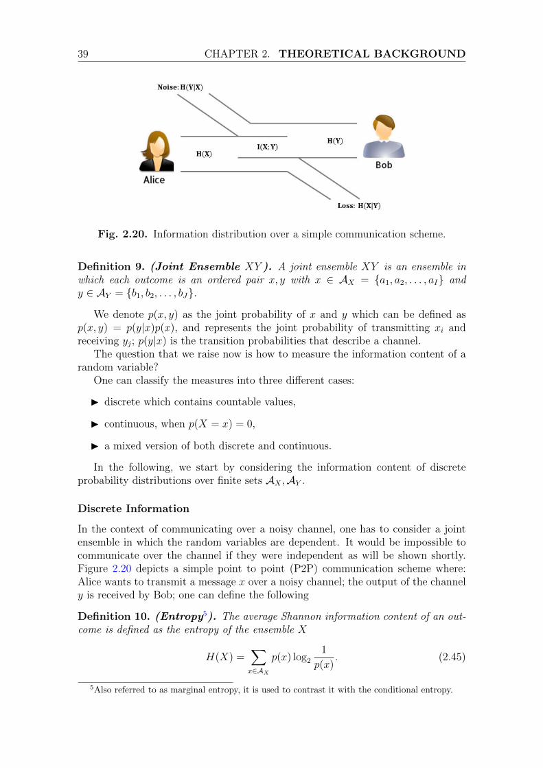
39 CHAPTER 2. THEORETICAL BACKGROUND
Fig. 2.20. Information distribution over a simple communication scheme.
Definition 9. (Joint Ensemble XY ). A joint ensemble XY is an ensemble inwhich each outcome is an ordered pair x, y with x ∈ AX = a1, a2, . . . , aI andy ∈ AY = b1, b2, . . . , bJ.
We denote p(x, y) as the joint probability of x and y which can be defined asp(x, y) = p(y|x)p(x), and represents the joint probability of transmitting xi andreceiving yj; p(y|x) is the transition probabilities that describe a channel.
The question that we raise now is how to measure the information content of arandom variable?
One can classify the measures into three different cases:
I discrete which contains countable values,
I continuous, when p(X = x) = 0,
I a mixed version of both discrete and continuous.
In the following, we start by considering the information content of discreteprobability distributions over finite sets AX ,AY .
Discrete Information
In the context of communicating over a noisy channel, one has to consider a jointensemble in which the random variables are dependent. It would be impossible tocommunicate over the channel if they were independent as will be shown shortly.Figure 2.20 depicts a simple point to point (P2P) communication scheme where:Alice wants to transmit a message x over a noisy channel; the output of the channely is received by Bob; one can define the following
Definition 10. (Entropy5). The average Shannon information content of an out-come is defined as the entropy of the ensemble X
H(X) =∑x∈AX
p(x) log2
1
p(x). (2.45)
5Also referred to as marginal entropy, it is used to contrast it with the conditional entropy.
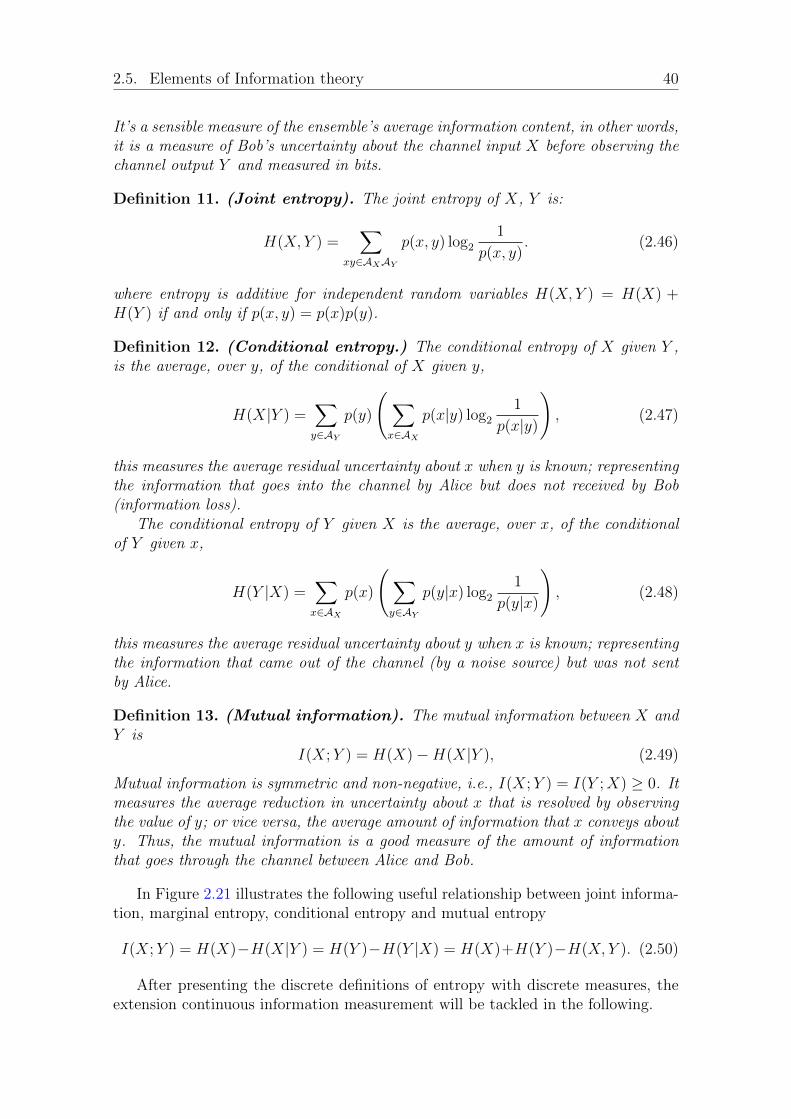
2.5. Elements of Information theory 40
It’s a sensible measure of the ensemble’s average information content, in other words,it is a measure of Bob’s uncertainty about the channel input X before observing thechannel output Y and measured in bits.
Definition 11. (Joint entropy). The joint entropy of X, Y is:
H(X, Y ) =∑
xy∈AXAY
p(x, y) log2
1
p(x, y). (2.46)
where entropy is additive for independent random variables H(X, Y ) = H(X) +H(Y ) if and only if p(x, y) = p(x)p(y).
Definition 12. (Conditional entropy.) The conditional entropy of X given Y ,is the average, over y, of the conditional of X given y,
H(X|Y ) =∑y∈AY
p(y)
(∑x∈AX
p(x|y) log2
1
p(x|y)
), (2.47)
this measures the average residual uncertainty about x when y is known; representingthe information that goes into the channel by Alice but does not received by Bob(information loss).
The conditional entropy of Y given X is the average, over x, of the conditionalof Y given x,
H(Y |X) =∑x∈AX
p(x)
(∑y∈AY
p(y|x) log2
1
p(y|x)
), (2.48)
this measures the average residual uncertainty about y when x is known; representingthe information that came out of the channel (by a noise source) but was not sentby Alice.
Definition 13. (Mutual information). The mutual information between X andY is
I(X;Y ) = H(X)−H(X|Y ), (2.49)
Mutual information is symmetric and non-negative, i.e., I(X;Y ) = I(Y ;X) ≥ 0. Itmeasures the average reduction in uncertainty about x that is resolved by observingthe value of y; or vice versa, the average amount of information that x conveys abouty. Thus, the mutual information is a good measure of the amount of informationthat goes through the channel between Alice and Bob.
In Figure 2.21 illustrates the following useful relationship between joint informa-tion, marginal entropy, conditional entropy and mutual entropy
I(X;Y ) = H(X)−H(X|Y ) = H(Y )−H(Y |X) = H(X)+H(Y )−H(X, Y ). (2.50)
After presenting the discrete definitions of entropy with discrete measures, theextension continuous information measurement will be tackled in the following.

41 CHAPTER 2. THEORETICAL BACKGROUND
Fig. 2.21. The relationship between joint information, marginal entropy, condi-tional entropy and mutual entropy.
Continuous Information
One may ask, what if the signals or messages we wish to transfer are a continuousvariable. Indeed, many practical channels have real, rather than discrete, inputsand outputs;
From the discrete case we can obtain the results for the continuous case as alimiting process. Consider a random variable X with an outcome xk = kδx for k =0,±1,±2, . . . having probability p(xk)δx, where p(xk) represents the probabilitydensity function that satisfy
∑k p(xk)δx=1.
By taking the limit of the discrete entropy formula of H(X) given in (2.45) weobtain
H(X) = limδx→0
∑k
p(xk)δx log2
(1
p(xk)δx
)
= limδx→0
[∑k
p(xk) log2
(1
p(xk)
)δx− log2(δx)
∑k
p(xk)δx
]
=
∫ ∞−∞
p(xk) log2
(1
p(x)
)dx−
(limδx→0
log2(δx))×∫ ∞−∞
p(x)dx
= h(X)− limδx→0
log2(δx) (2.51)
This is rather worrying as the second term does not exist. However, as we areoften interested in the differences between entropies in the consideration of mutualentropy or capacity we define the problem by using the first term only as a measureof differential entropy6.
Hence, we can now define also the joint and conditional entropies for continuous
6Differential entropy is not a measure of the average amount of information contained in acontinuous random variable (in general, it contains an infinite amount of information).

2.5. Elements of Information theory 42
distributions:
h(X, Y ) =
∫Y
∫X
p(x, y) log2
(1
p(x, y)
)dxdy (2.52)
h(X|Y ) =
∫Y
∫X
p(x, y) log2
(p(y)
p(x, y)
)dxdy (2.53)
h(Y |X) =
∫Y
∫X
p(x, y) log2
(p(x)
p(x, y)
)dxdy (2.54)
with:
p(x) =
∫Y
p(x, y)dy (2.55)
p(y) =
∫X
p(x, y)dx (2.56)
Eventually, the mutual information between two continuous random variable X andY is defined as
I(X, Y ) =
∫Y
∫X
p(x, y) log2
(p(x|y)
p(x)
)dxdy (2.57)
Channel capacity
The mutual information relies on both the channel characteristics (represented bythe conditional probability distribution) and the input probability distribution,which is clearly independent of the channel7. Therefore, by changing the inputprobability distribution, the average mutual information will change. Let us assumethat we want to maximize the mutual information that goes through the channel bychoosing the best possible input ensemble, one can note that it is possible to findmultiple optimal input distributions achieving the same value of I(X;Y ). We candefine the channel capacity to be its maximum mutual information
C = supPX
I(X;Y ). (2.58)
Under the input average power constraint the r.v. X satisfies E[X2i ] ≤ P . The
capacity is determined by the intrinsic properties of the channel and is independentof the content of the transmitted information and the way it is encoded.
For any binary memory less symmetric channels one can compute the capacityas a function of LLR’s [RU08].
Lemma 2. (Capacity MBISO channels.) Let f be the density associated witha MBISO channel. Then the capacity of this channel in bits per channel use is
C = 1− E[log2
(1 + e−XΛ(Y )
)](2.59)
7let p(y|x) be the conditional probability distribution of y given x, which is an inherent fixedproperty of the communication channel. Then the choice of the marginal distribution p(x) com-pletely determines the joint distribution p(x, y) due to the identity p(x, y) = p(y|x)p(x) which, inturn induces a mutual information.

43 CHAPTER 2. THEORETICAL BACKGROUND
Proof.
C = H(Y )−H(Y |X)
=
∫Y
P (y) log2
(1
P (y)
)dy −
∑x=±1
P (x)
(∫Y
P (y|x) log2
(1
P (y|x)
)dy
)=
∫Y
1
2
∑x=±1
P (y|x) log2
(2P (y|x)
P (y|1) + P (y| − 1)
)dy
=
∫Y
P (y|1) log2
(2P (y|1)
P (y|1) + P (y| − 1)
)dy (2.60)
where for the transition to the fourth line we have used Definition 7 (page 38) for asymmetric channel P (y|1) = P (−y| − 1).
Let f(y) be the probability density at the channel output y when x = 1 istransmitted. Then, P (y|1) = f(y) and P (y| − 1) = f(−y). The logarithm of thelikelihood ratio LLR8 Λ(y) then takes the following particular expression:
Λ(y) = logP (y|+ 1)
P (y| − 1)= log
f(y)
f(−y)(2.61)
from (2.61) we can obtain f(−y) = f(y)e−Λ(y), replacing it in (2.60) gives
C =
∫Y
f(y) log2
(2f(y)
f(y) + f(−y)
)dy
=
∫Y
f(y) log2
(2
1 + e−Λ(y)
)dy
=
∫Y
f(y)dy −∫Y
f(y) log2
(1 + e−Λ(y)
)dy
= 1− EY[log2
(1 + e−Λ(Y )
)]. (2.62)
By considering the two possible input values +1 or −1, (2.62) becomes
C = 1− EY[log2
(1 + e−XΛ(Y )
)]. (2.63)
2.6 Capacity for MBISO channels
The channel capacity is an extremely important quantity since it is possible totransmit information through a channel at any rate less than the channel capacitywith an arbitrarily small probability of error; completely reliable transmission is not
8The LLR is a prime tool in information theory as it constitutes a sufficient statistic relativeto the channel input [RU08]; in other words, knowing Λ(Y ) or Y is equivalent for the decodingprocess.
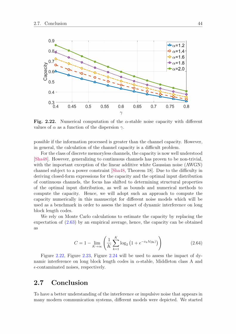
2.7. Conclusion 44
Fig. 2.22. Numerical computation of the α-stable noise capacity with differentvalues of α as a function of the dispersion γ.
possible if the information processed is greater than the channel capacity. However,in general, the calculation of the channel capacity is a difficult problem.
For the class of discrete memoryless channels, the capacity is now well understood[Sha48]. However, generalizing to continuous channels has proven to be non-trivial,with the important exception of the linear additive white Gaussian noise (AWGN)channel subject to a power constraint [Sha48, Theorem 18]. Due to the difficulty inderiving closed-form expressions for the capacity and the optimal input distributionof continuous channels, the focus has shifted to determining structural propertiesof the optimal input distribution, as well as bounds and numerical methods tocompute the capacity. Hence, we will adopt such an approach to compute thecapacity numerically in this manuscript for different noise models which will beused as a benchmark in order to assess the impact of dynamic interference on longblock length codes.
We rely on Monte Carlo calculations to estimate the capacity by replacing theexpectation of (2.63) by an empirical average, hence, the capacity can be obtainedas
C = 1− limK→∞
(1
K
K∑k=1
log2
(1 + e−xkΛ(yk)
))(2.64)
Figure 2.22, Figure 2.23, Figure 2.24 will be used to assess the impact of dy-namic interference on long block length codes in α-stable, Middleton class A andε-contaminated noises, respectively.
2.7 Conclusion
To have a better understanding of the interference or impulsive noise that appears inmany modern communication systems, different models were depicted. We started
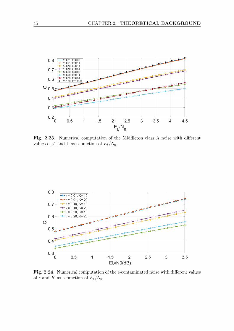
45 CHAPTER 2. THEORETICAL BACKGROUND
Fig. 2.23. Numerical computation of the Middleton class A noise with differentvalues of A and Γ as a function of Eb/N0.
Fig. 2.24. Numerical computation of the ε-contaminated noise with different valuesof ε and K as a function of Eb/N0.
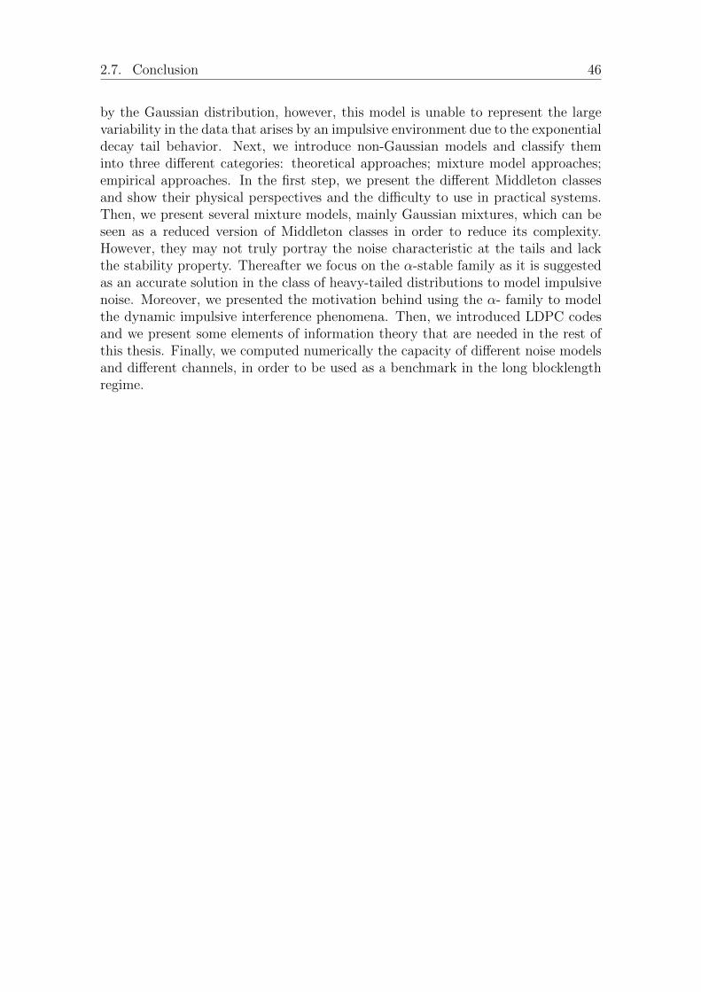
2.7. Conclusion 46
by the Gaussian distribution, however, this model is unable to represent the largevariability in the data that arises by an impulsive environment due to the exponentialdecay tail behavior. Next, we introduce non-Gaussian models and classify theminto three different categories: theoretical approaches; mixture model approaches;empirical approaches. In the first step, we present the different Middleton classesand show their physical perspectives and the difficulty to use in practical systems.Then, we present several mixture models, mainly Gaussian mixtures, which can beseen as a reduced version of Middleton classes in order to reduce its complexity.However, they may not truly portray the noise characteristic at the tails and lackthe stability property. Thereafter we focus on the α-stable family as it is suggestedas an accurate solution in the class of heavy-tailed distributions to model impulsivenoise. Moreover, we presented the motivation behind using the α- family to modelthe dynamic impulsive interference phenomena. Then, we introduced LDPC codesand we present some elements of information theory that are needed in the rest ofthis thesis. Finally, we computed numerically the capacity of different noise modelsand different channels, in order to be used as a benchmark in the long blocklengthregime.

Chapter 3Robust Receiver Design
Establishing reliable and efficient communications require to take into account theimpulsive nature while designing the receivers. The interference modeling questionwas answered in the aforementioned part; it exhibits in many situations an impul-sive behavior. Without being exhaustive we presented several approaches adapted tospecific situations. However, designing a specific receiver for each situation is notefficient as the interference characteristics can highly vary in time and space. Thus,having a receiver able to cope with a large set of different interference models (impul-sive or not) and with different degrees of impulsiveness is highly desired. This is themain challenge we address in this manuscript. For this purpose, we start by clarify-ing the impact of impulsive interference on the optimal decision regions. Then, weclassify the different receiver design approaches seen in the literature. Thereafter, weintroduce the system scenario and propose a new framework inspired by informationtheory for the sake of designing a robust receiver.
3.1 Impact of impulsive interference on optimal
decision regions
An efficient way to characterize and understand the influence of impulsive noise isto visualize the noise impact on the optimal receiver by representing the decision
regions. This was proposed by Saaifan and Henkel [SH13] for the Middleton classA case and by Shehat et al. [SME10] and by Saleh et al. [SME12] for the α-stablecase.
We represent in Figure 3.1 six different examples of noise realizations from im-pulsive noise models. We follow the framework proposed in [SME12] and use thesame parameters defined in Figure 3.1: the received vector Y is composed of tworeceived samples (two dimensions, Y = [y1, y2]), and we consider two possible trans-mitted values x ∈ Ω = −1, 1. Then we show in Figure 3.2 the decision regions rthat the optimal receiver must produce in a binary case under different interferencemodels, i.e., the regions that maximize the probability of having transmitted x whenY = (y1, y2) = (x+n1, x+n2) is received with two i.i.d. impulsive noise realizations
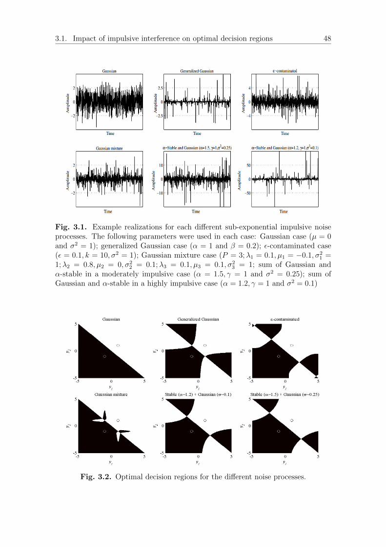
3.1. Impact of impulsive interference on optimal decision regions 48
Fig. 3.1. Example realizations for each different sub-exponential impulsive noiseprocesses. The following parameters were used in each case: Gaussian case (µ = 0and σ2 = 1); generalized Gaussian case (α = 1 and β = 0.2); ε-contaminated case(ε = 0.1, k = 10, σ2 = 1); Gaussian mixture case (P = 3;λ1 = 0.1, µ1 = −0.1, σ2
1 =1;λ2 = 0.8, µ2 = 0, σ2
2 = 0.1;λ3 = 0.1, µ3 = 0.1, σ23 = 1; sum of Gaussian and
α-stable in a moderately impulsive case (α = 1.5, γ = 1 and σ2 = 0.25); sum ofGaussian and α-stable in a highly impulsive case (α = 1.2, γ = 1 and σ2 = 0.1)
Fig. 3.2. Optimal decision regions for the different noise processes.
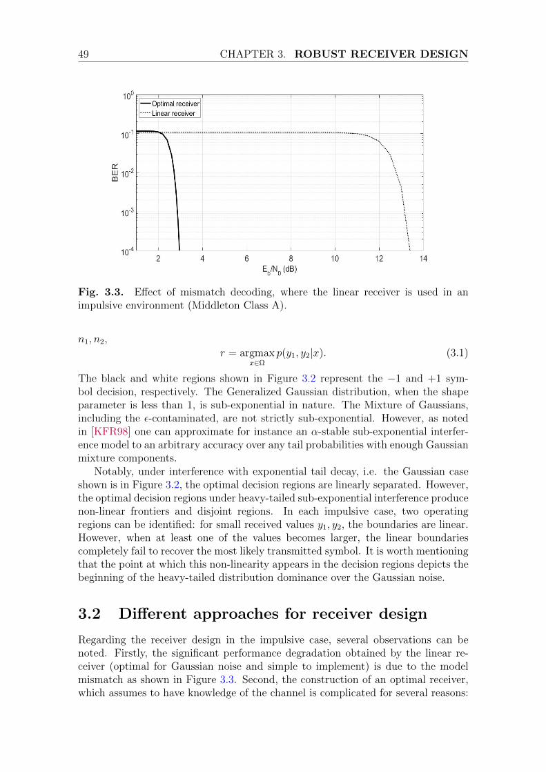
49 CHAPTER 3. ROBUST RECEIVER DESIGN
Fig. 3.3. Effect of mismatch decoding, where the linear receiver is used in animpulsive environment (Middleton Class A).
n1, n2,
r = argmaxx∈Ω
p(y1, y2|x). (3.1)
The black and white regions shown in Figure 3.2 represent the −1 and +1 sym-bol decision, respectively. The Generalized Gaussian distribution, when the shapeparameter is less than 1, is sub-exponential in nature. The Mixture of Gaussians,including the ε-contaminated, are not strictly sub-exponential. However, as notedin [KFR98] one can approximate for instance an α-stable sub-exponential interfer-ence model to an arbitrary accuracy over any tail probabilities with enough Gaussianmixture components.
Notably, under interference with exponential tail decay, i.e. the Gaussian caseshown is in Figure 3.2, the optimal decision regions are linearly separated. However,the optimal decision regions under heavy-tailed sub-exponential interference producenon-linear frontiers and disjoint regions. In each impulsive case, two operatingregions can be identified: for small received values y1, y2, the boundaries are linear.However, when at least one of the values becomes larger, the linear boundariescompletely fail to recover the most likely transmitted symbol. It is worth mentioningthat the point at which this non-linearity appears in the decision regions depicts thebeginning of the heavy-tailed distribution dominance over the Gaussian noise.
3.2 Different approaches for receiver design
Regarding the receiver design in the impulsive case, several observations can benoted. Firstly, the significant performance degradation obtained by the linear re-ceiver (optimal for Gaussian noise and simple to implement) is due to the modelmismatch as shown in Figure 3.3. Second, the construction of an optimal receiver,which assumes to have knowledge of the channel is complicated for several reasons:
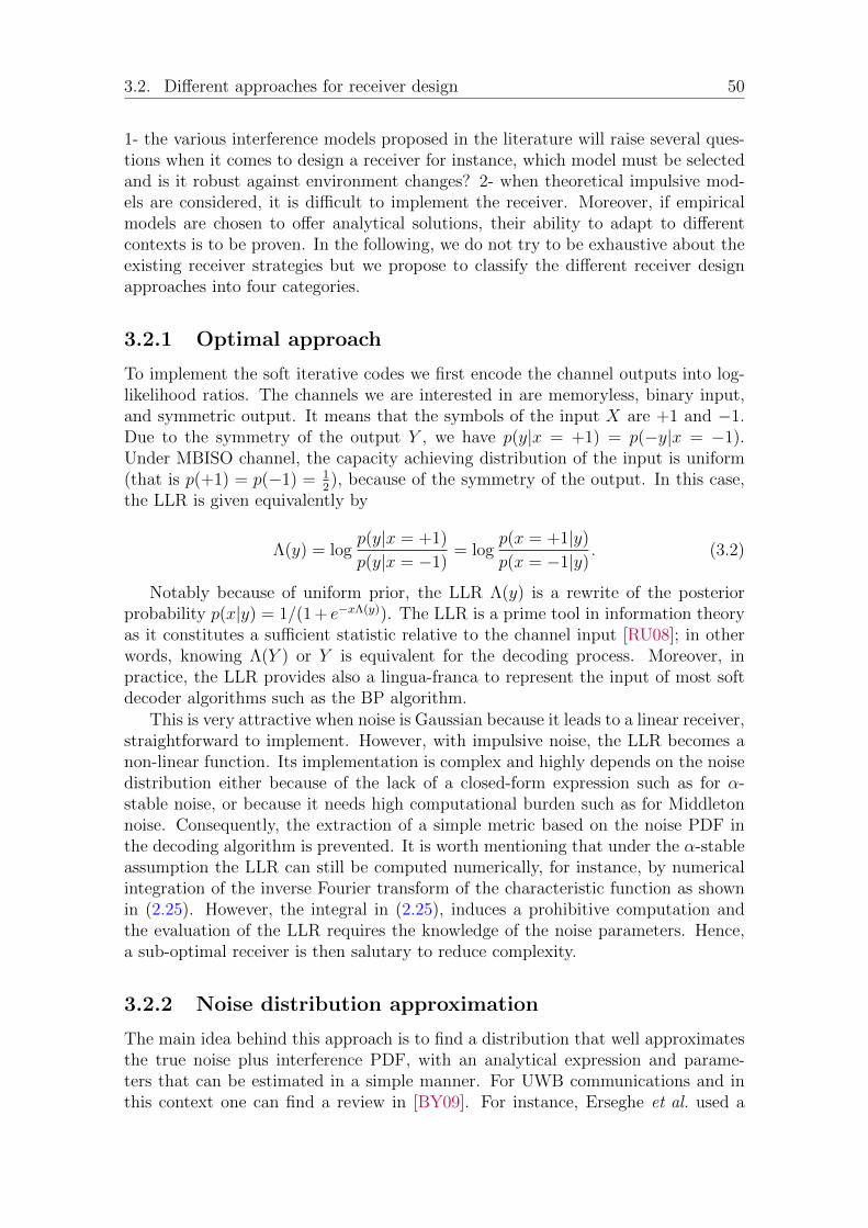
3.2. Different approaches for receiver design 50
1- the various interference models proposed in the literature will raise several ques-tions when it comes to design a receiver for instance, which model must be selectedand is it robust against environment changes? 2- when theoretical impulsive mod-els are considered, it is difficult to implement the receiver. Moreover, if empiricalmodels are chosen to offer analytical solutions, their ability to adapt to differentcontexts is to be proven. In the following, we do not try to be exhaustive about theexisting receiver strategies but we propose to classify the different receiver designapproaches into four categories.
3.2.1 Optimal approach
To implement the soft iterative codes we first encode the channel outputs into log-likelihood ratios. The channels we are interested in are memoryless, binary input,and symmetric output. It means that the symbols of the input X are +1 and −1.Due to the symmetry of the output Y , we have p(y|x = +1) = p(−y|x = −1).Under MBISO channel, the capacity achieving distribution of the input is uniform(that is p(+1) = p(−1) = 1
2), because of the symmetry of the output. In this case,
the LLR is given equivalently by
Λ(y) = logp(y|x = +1)
p(y|x = −1)= log
p(x = +1|y)
p(x = −1|y). (3.2)
Notably because of uniform prior, the LLR Λ(y) is a rewrite of the posteriorprobability p(x|y) = 1/(1 + e−xΛ(y)). The LLR is a prime tool in information theoryas it constitutes a sufficient statistic relative to the channel input [RU08]; in otherwords, knowing Λ(Y ) or Y is equivalent for the decoding process. Moreover, inpractice, the LLR provides also a lingua-franca to represent the input of most softdecoder algorithms such as the BP algorithm.
This is very attractive when noise is Gaussian because it leads to a linear receiver,straightforward to implement. However, with impulsive noise, the LLR becomes anon-linear function. Its implementation is complex and highly depends on the noisedistribution either because of the lack of a closed-form expression such as for α-stable noise, or because it needs high computational burden such as for Middletonnoise. Consequently, the extraction of a simple metric based on the noise PDF inthe decoding algorithm is prevented. It is worth mentioning that under the α-stableassumption the LLR can still be computed numerically, for instance, by numericalintegration of the inverse Fourier transform of the characteristic function as shownin (2.25). However, the integral in (2.25), induces a prohibitive computation andthe evaluation of the LLR requires the knowledge of the noise parameters. Hence,a sub-optimal receiver is then salutary to reduce complexity.
3.2.2 Noise distribution approximation
The main idea behind this approach is to find a distribution that well approximatesthe true noise plus interference PDF, with an analytical expression and parame-ters that can be estimated in a simple manner. For UWB communications and inthis context one can find a review in [BY09]. For instance, Erseghe et al. used a
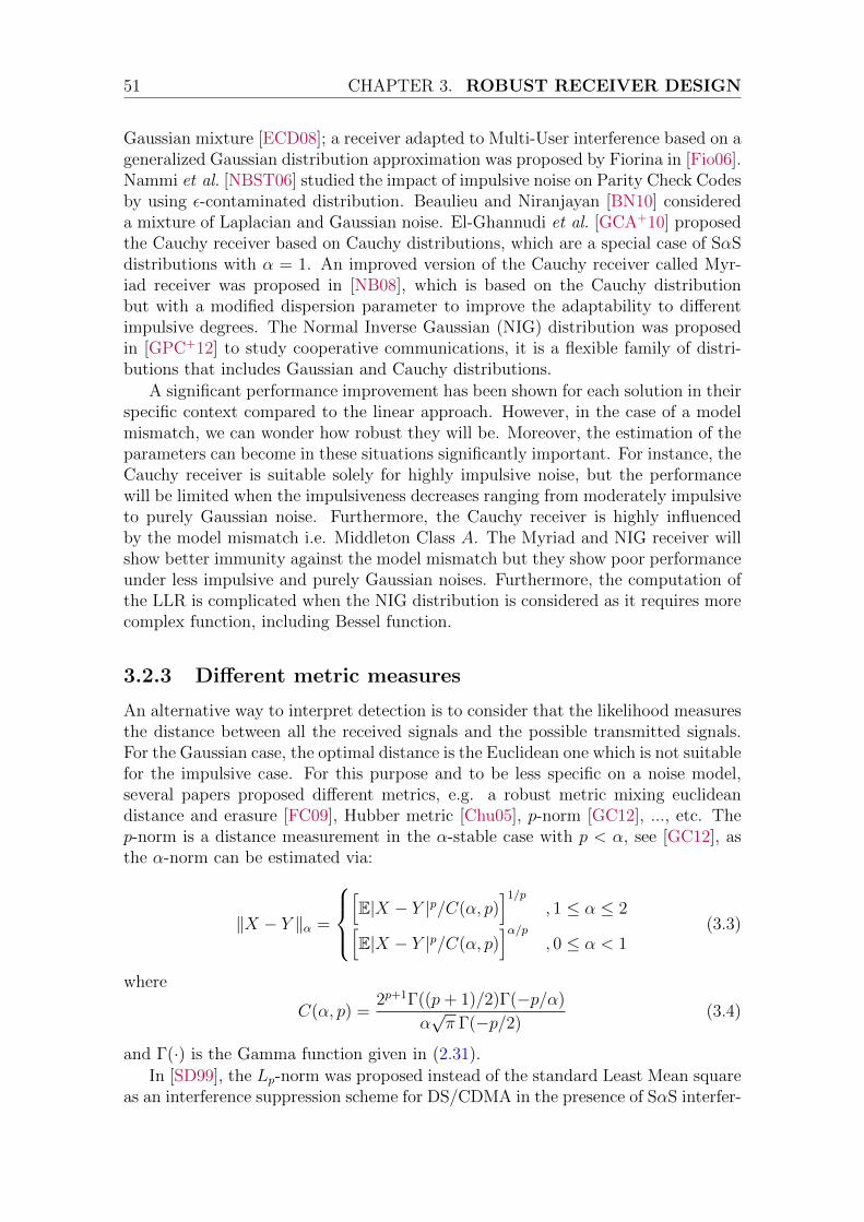
51 CHAPTER 3. ROBUST RECEIVER DESIGN
Gaussian mixture [ECD08]; a receiver adapted to Multi-User interference based on ageneralized Gaussian distribution approximation was proposed by Fiorina in [Fio06].Nammi et al. [NBST06] studied the impact of impulsive noise on Parity Check Codesby using ε-contaminated distribution. Beaulieu and Niranjayan [BN10] considereda mixture of Laplacian and Gaussian noise. El-Ghannudi et al. [GCA+10] proposedthe Cauchy receiver based on Cauchy distributions, which are a special case of SαSdistributions with α = 1. An improved version of the Cauchy receiver called Myr-iad receiver was proposed in [NB08], which is based on the Cauchy distributionbut with a modified dispersion parameter to improve the adaptability to differentimpulsive degrees. The Normal Inverse Gaussian (NIG) distribution was proposedin [GPC+12] to study cooperative communications, it is a flexible family of distri-butions that includes Gaussian and Cauchy distributions.
A significant performance improvement has been shown for each solution in theirspecific context compared to the linear approach. However, in the case of a modelmismatch, we can wonder how robust they will be. Moreover, the estimation of theparameters can become in these situations significantly important. For instance, theCauchy receiver is suitable solely for highly impulsive noise, but the performancewill be limited when the impulsiveness decreases ranging from moderately impulsiveto purely Gaussian noise. Furthermore, the Cauchy receiver is highly influencedby the model mismatch i.e. Middleton Class A. The Myriad and NIG receiver willshow better immunity against the model mismatch but they show poor performanceunder less impulsive and purely Gaussian noises. Furthermore, the computation ofthe LLR is complicated when the NIG distribution is considered as it requires morecomplex function, including Bessel function.
3.2.3 Different metric measures
An alternative way to interpret detection is to consider that the likelihood measuresthe distance between all the received signals and the possible transmitted signals.For the Gaussian case, the optimal distance is the Euclidean one which is not suitablefor the impulsive case. For this purpose and to be less specific on a noise model,several papers proposed different metrics, e.g. a robust metric mixing euclideandistance and erasure [FC09], Hubber metric [Chu05], p-norm [GC12], ..., etc. Thep-norm is a distance measurement in the α-stable case with p < α, see [GC12], asthe α-norm can be estimated via:
‖X − Y ‖α =
[E|X − Y |p/C(α, p)
]1/p
, 1 ≤ α ≤ 2[E|X − Y |p/C(α, p)
]α/p, 0 ≤ α < 1
(3.3)
where
C(α, p) =2p+1Γ((p+ 1)/2)Γ(−p/α)
α√π Γ(−p/2)
(3.4)
and Γ(·) is the Gamma function given in (2.31).
In [SD99], the Lp-norm was proposed instead of the standard Least Mean squareas an interference suppression scheme for DS/CDMA in the presence of SαS interfer-

3.2. Different approaches for receiver design 52
ence. The decision statistic for the p-norm metric is given without the normalizationconstant by
L(y) = |y − 1|p − |y + 1|p. (3.5)
Attractively, only a rough knowledge of α is needed and there is no need for anydistribution parameter estimation. However, the estimation of the p value will playa significant role in terms of performance.
3.2.4 Direct LLR approximation
Linear approximation: evaluating the LLR with a Gaussian noise assumptionresults in a linear operation for detection and is denoted as the linear receiver. Weprimarily consider this choice for its simple implementation structure and also as areference to show the gain achieved by using other approaches, though it is known toperform poorly in impulsive situations. The LLR for the Gaussian noise is expressedby:
ΛG(y) = logfN(y − 1)
fN(y + 1),
= loge−(y−1)2/2σ2
e−(y+1)2/2σ2 =2y
σ2. (3.6)
where fN(·) denotes the PDF (2.3) of the noise N and σ is the standard deviation.Using only a linear scaling whose slope depends on the additive noise variance
leads to severe performance loss as soon as noise is impulsive. This performanceloss occurs because with this linear scaling, large values in Y result into large LLR.However, under impulsive noise, large values in Y are more likely due to an impulsiveevent (meaning a less reliable sample) so that the LLR should be small.
Non-linear LLR approximation: under impulsive noise, the LLR is computa-tionally prohibitive as discussed in Section 3.2.1, consequently, we consider para-metric approximation Lθ of the LLR Λ(y). The family of functions Lθ is chosen forits simplicity and for its flexibility to represent the LLR of different channel types.Besides, if we consider a family defined by a limited number of parameters andeasy to be implemented, both the estimation and implementation complexities arereduced. Hence, to narrow down the search space and to have an easy to implementapproximation, we assume that the estimated LLR Lθ is an odd piece-wise functionof the optimization parameter θ. More precisely, we are interested in functions thatcan be represented as
Lθ(y) = sign(y) min θ1φ1(|y|), θ2φ2(|y|), . . . , θnφn(|y|) , (3.7)
where sign(x) is defined as sign(x) = x/ |x|; φi(|y|) are functions depending solelyon the channel output |y| but not necessarily linear in |y|; the parameter θ, givenas θ = [θ1, θ2, . . . , θn] ∈ Rn
+, is the the optimization parameter that needs to beestimated. This formulation includes the linear case. The family of function is then

53 CHAPTER 3. ROBUST RECEIVER DESIGN
Fig. 3.4. LLR demapper for α = 1.4, γ = 0.5, and its approximation.
simply Lθ(y) = ay, this is called thereafter the La receiver. The formulation (3.7)allows us to take into account asymptotical approximations of the LLR.
Figure 3.4 lightens the non-linearity of the LLR function for the channel outputY when the noise is α-stable. At a first look, two different parts in the LLR can beobserved: a first one when y is close to zero and another one when y becomes largeenough. When y is close to zero, the LLR is almost linear, whereas when y is largeenough, the LLR presents a power-law decrease. When the noise is Gaussian, thelinear region spreads with the decrease of the noise impulsiveness until reaching thelimit (only the linear part exists).
Remark 2. Even if Figure 3.4 delineates a specific noise model (α-stable), theoverall appearance of the LLR exhibits a similar behavior for other impulsive models.
The presence of these two parts has been used in the literature to propose severalLLR approximations [DGCG14, AIH94, MGCG13, SMET12, MSG+18] and justifiesthe proposed piece-wise affine set for the LLRs approximation. Firstly, severalapproximations cope with impulses by limiting the received values such as soft limiterand hole-puncher [AIH94]. In [MGCG13], a variant of the soft limiter was proposedcalled the clipper, where the LLR equation is:
Lclipp(y) =
py if −h/p < y < h/p
h sign(y) otherwise,(3.8)
where p represents the signal amplitude and the impulse clipping level is representedby h, using the density evolution they obtain both parameters. The clipper demap-per also falls into the formulation (3.7). In order to match the parametric notationdefined in (3.7), the clipper demapper can be rewritten as:
Lclip(y) = sgn(y) min(a|y|,
√ab)
=
ay if |y| <
√b/a,√
ab otherwise,(3.9)

3.2. Different approaches for receiver design 54
Fig. 3.5. The demapper scheme.
where a represent the slope of the linear part and√ab represent the clipping thresh-
old.Despite the performance improvement seen in the clipping receiver compared to
the linear one, we expect that approximating the optimal LLR might give a near-optimal performance. Indeed, recently the approximated LLR receiver [DGCG14]which will be called thereafter Lab was proposed. The Lab demapper decomposesthe LLR into two parts: a linear part and an asymptotic part. The linear partis proportional to the received signal and is related to the noise dispersion γ andthe asymptotic part is derived from the asymptotic expansion approximation ofthe density function of stable variable proposition 2 (page 27) and it reflects theheaviness of the tail. Hence, the Lab demapper is given by
Lab(y) = sgn(y) min(a|y|, b/|y|
)=
ay if |y| <
√b/a,
b/y otherwise,(3.10)
where a =√
2/γ and b = 2(α + 1). Remark that, the demapper may be directlyparameterized by a and b instead of α and γ.
Recently, we proposed [MSG+19c] a new approximation based on three param-eters which will be called thereafter Labc, expecting to have an approximation thatfits the true LLR to a high degree without adding much complexity. Consequently,near-optimum performance can be achieved. Hence, the Labc demapper is given by
Labc(y) = sgn(y) min(a|y|, b/|y|, c
)=
ay if |y| < c/a,
c if c/a < |y| > bc,
b/y if |y| > bc,
(3.11)
where a represents the slope of the linear part (for small values of y), b representsthe degree of decay of the asymptotic part (for large values of y) and c represents asaturation level. The Labc demapper will be further detailed in Section 4.2.3.
This thesis mainly deals with this transformation between channel output anddecoder input. This transformation is called thereafter demapping as shown inFigure 3.5. Attractively, constructing an adaptive robust receiver in a way that canbe used at the front end of any LLR-based decoder will be of great advantage as itcan be migrated to any LLR-based decoder like LDPC, turbo, etc.
The main question arising after having chosen the parametric function Lθ, ishow to estimate θ in order to minimize the BER or the Frame Error Rate (FER)?For this purpose, we study in the following different methods.

55 CHAPTER 3. ROBUST RECEIVER DESIGN
3.3 Different parameter optimization methods
The approximated LLRs require the knowledge of the parameter θ in order to betuned and match the channel state. The first idea to estimate these parameters isto compute them directly from noise samples—which may be obtained by a trainingsequence. We can mention three methods to estimate these parameters:
I direct estimation of the noise model parameters α and γ and then takinga =√
2/γ and b = 2(α + 1). This is equivalent to considering that the noisedistribution follows an α-stable law. Two different methods are used to esti-mate the parameters of the stable distribution: the first is based on quantilesproposed by McCulloch [McC86b] and the second use regression type estima-tion method based on the characteristic function proposed by Koutrouvelisin [Kou81]. Apparently, the performance in terms of BER of such methodswill be degraded as the environment changes due to the noise model mismatcheffect.
I direct noise distribution estimation: in this case, a kernel density estimationis used followed by fitting the estimated LLR (L(x)) with the approximationLab: first the noise PDF will be estimated using some classical kernel-basedapproaches. Thereafter, by using the density estimation, the LLR is estimateddirectly by computing (3.2). Unfortunately, L(x) is difficult to use as an on-line real-time likelihood approximation. This is essentially due to missingsamples which results in the appearance of zeros in the density estimation.Consequently, the two parameters a and b will be estimated from L(x) by
considering its maximum (xm): a = L(xm)/xm and b = ax2m. It is worth
mentioning that such a method will be degenerated under some extreme situ-ations, for instance, when the noise magnitude is too small or when the noisesamples are too large.
I maximization of the mutual information between the source and the output ofthe approximated LLR: this approach is attractive since it does not assume aparticular noise-plus-interference model. It is inspired by the work of Yazdaniand Ardakani in [YA09]. In order to find the best slope of the linear receiver,they used the maximization of mutual information between the source and thereceiver output. Nevertheless, this approach can be adjusted easily in order tofit our estimation problem, in general, to find the optimal parameter θ∗ thatwill tune the demapper Lθ∗ and thus match the channel state. The receiverparameter θ∗ is now given by
θ∗ = argmaxθ
I(X;Lθ(Y )). (3.12)
This method will be studied in more detail in the rest of the manuscript.
3.4 Proposed framework and system scenario
Source: we use a LDPC code associated with a BP-decoding algorithm. This caseis well-suited to our proposal because the LLR has to be estimated and fed to the

3.5. Online real-time parameter estimation method 56
BP algorithm. Nevertheless, our solution is not limited to these codes but couldbe applied to any code families whose decoding relies on the LLR, as for instanceconvolutional codes or turbo-codes.
In the following, we study the proposed framework with two different blocklengths, long and short. We assume that the binary message X is encoded using aregular (3,6) LDPC code of length 20000 and 408, respectively. We did the samestudy over different LDPC codes, but the conclusions are the same.
Channel: the channels we are interested in are memoryless, binary input, andsymmetric output (MBISO). A large number of channels fall into this class such asthe Binary Symmetric Channel (BSC), the Binary Erasure Channel (BEC) or theAdditive White Gaussian Noise (AWGN) Channel. A wide range of situations can bedealt with rather straightforwardly once we have mastered MBISO channels [RU08].More generally, channels defined by Y = X +N , whose inputs X are perturbed byan additive noise N belong to the MBISO family as long as the additive pertur-bations are symmetric and independent from the input. The noise may representthermal noise but also impulsive interference. In the latter, N can be modeled,for instance, by a Middleton class A distribution [Mid77] or a symmetric α-stabledistribution [PW10a], etc. In particular, we will focus on Symmetric α stable (SαS)distributions. Nevertheless, we also want to check the robustness against differentnoise models. Consequently, we will study the behavior of our approach with otherclassical noise models: Gaussian, Middleton class A and ε−contaminated.
Receiver: thereafter, we will adopt the Lab demapper for further study andanalysis since it outperforms the most used LLR approximations [HLZ14,MJLC15].This work can be extended with more or less efforts to other approximations or tohigher modulation schemes.
Parameter optimization method: we aim at the smallest BER and FER; butthis criterion is not within reach in practice. Moreover, we constraint ourselves tohave a criterion that can be used directly at the receiver (to achieve online real-timeparameter estimation) which requires: simple implementation and fast learning (onthe fly) in order to match practical receiver implementation. We propose to estimatethe LLR approximation parameters by maximizing the mutual information betweenthe source and the channel output (3.14). This does not rely on the knowledge of thenoise distribution. We consequently expect robustness of this approach in differentinterference contexts. The justification of such an approach will be tackled in thefollowing.
3.5 Online real-time parameter estimation method
The LLR approximations depend on several parameters, grouped here under thevariable θ, which must be optimized to make the approximation as close as possibleto the LLR.
3.5.1 LLR approximation as an optimization problem
We propose to perform the estimation under an information theory criterion basedon the capacity of MBISO channel, which can be expressed as a function of the
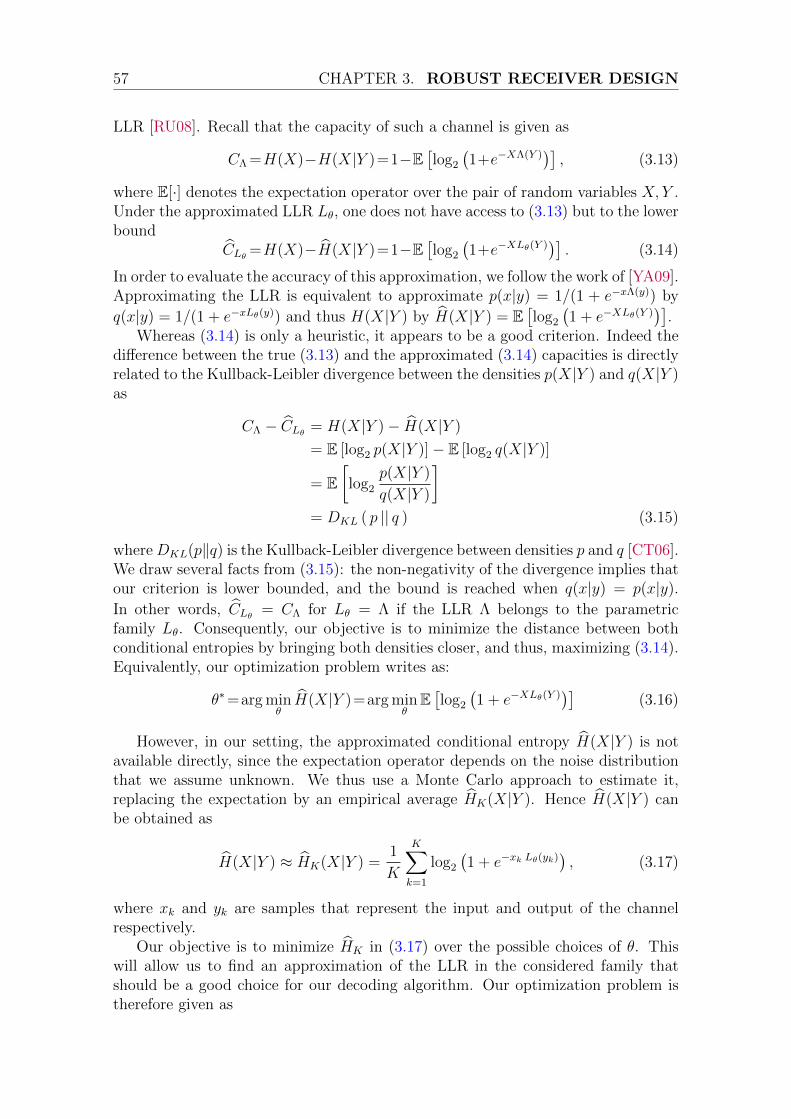
57 CHAPTER 3. ROBUST RECEIVER DESIGN
LLR [RU08]. Recall that the capacity of such a channel is given as
CΛ =H(X)−H(X|Y )=1−E[log2
(1+e−XΛ(Y )
)], (3.13)
where E[·] denotes the expectation operator over the pair of random variables X, Y .Under the approximated LLR Lθ, one does not have access to (3.13) but to the lowerbound
CLθ =H(X)−H(X|Y )=1−E[log2
(1+e−XLθ(Y )
)]. (3.14)
In order to evaluate the accuracy of this approximation, we follow the work of [YA09].Approximating the LLR is equivalent to approximate p(x|y) = 1/(1 + e−xΛ(y)) by
q(x|y) = 1/(1 + e−xLθ(y)) and thus H(X|Y ) by H(X|Y ) = E[log2
(1 + e−XLθ(Y )
)].
Whereas (3.14) is only a heuristic, it appears to be a good criterion. Indeed thedifference between the true (3.13) and the approximated (3.14) capacities is directlyrelated to the Kullback-Leibler divergence between the densities p(X|Y ) and q(X|Y )as
CΛ − CLθ = H(X|Y )− H(X|Y )
= E [log2 p(X|Y )]− E [log2 q(X|Y )]
= E[log2
p(X|Y )
q(X|Y )
]= DKL ( p || q ) (3.15)
whereDKL(p‖q) is the Kullback-Leibler divergence between densities p and q [CT06].We draw several facts from (3.15): the non-negativity of the divergence implies thatour criterion is lower bounded, and the bound is reached when q(x|y) = p(x|y).
In other words, CLθ = CΛ for Lθ = Λ if the LLR Λ belongs to the parametricfamily Lθ. Consequently, our objective is to minimize the distance between bothconditional entropies by bringing both densities closer, and thus, maximizing (3.14).Equivalently, our optimization problem writes as:
θ∗=arg minθH(X|Y )=arg min
θE[log2
(1 + e−XLθ(Y )
)](3.16)
However, in our setting, the approximated conditional entropy H(X|Y ) is notavailable directly, since the expectation operator depends on the noise distributionthat we assume unknown. We thus use a Monte Carlo approach to estimate it,replacing the expectation by an empirical average HK(X|Y ). Hence H(X|Y ) canbe obtained as
H(X|Y ) ≈ HK(X|Y ) =1
K
K∑k=1
log2
(1 + e−xk Lθ(yk)
), (3.17)
where xk and yk are samples that represent the input and output of the channelrespectively.
Our objective is to minimize HK in (3.17) over the possible choices of θ. Thiswill allow us to find an approximation of the LLR in the considered family thatshould be a good choice for our decoding algorithm. Our optimization problem istherefore given as
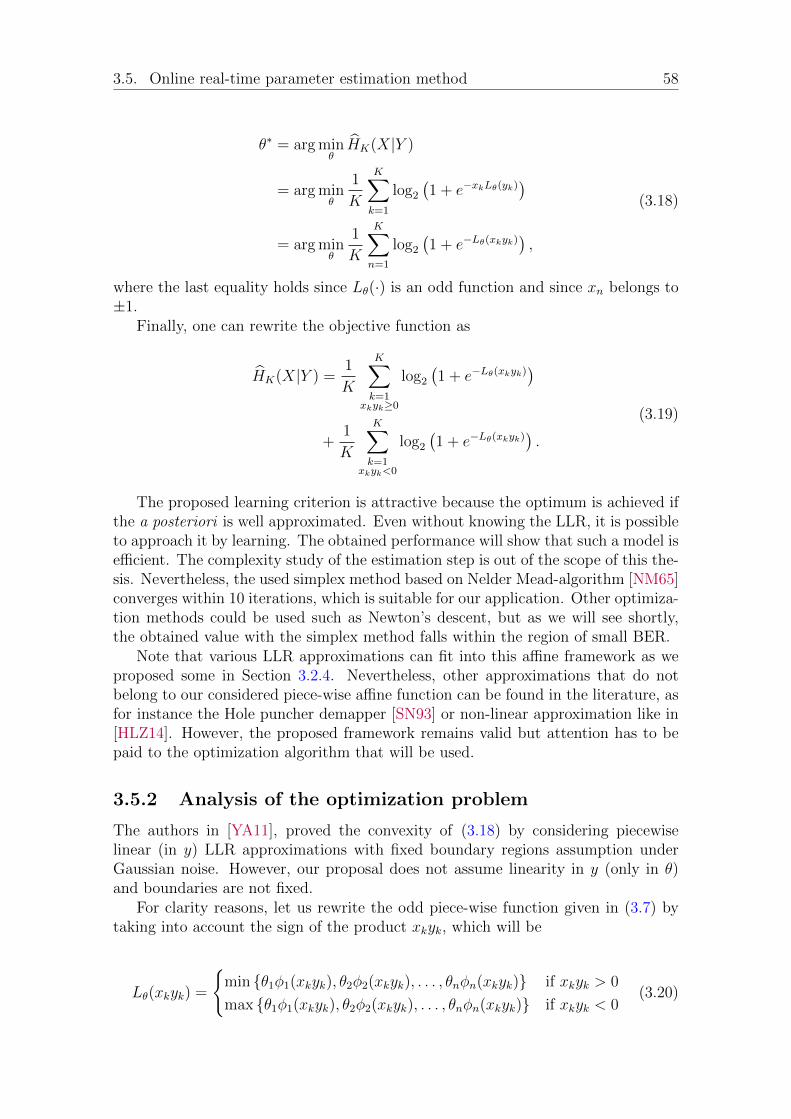
3.5. Online real-time parameter estimation method 58
θ∗ = arg minθHK(X|Y )
= arg minθ
1
K
K∑k=1
log2
(1 + e−xkLθ(yk)
)= arg min
θ
1
K
K∑n=1
log2
(1 + e−Lθ(xkyk)
),
(3.18)
where the last equality holds since Lθ(·) is an odd function and since xn belongs to±1.
Finally, one can rewrite the objective function as
HK(X|Y ) =1
K
K∑k=1
xkyk≥0
log2
(1 + e−Lθ(xkyk)
)
+1
K
K∑k=1
xkyk<0
log2
(1 + e−Lθ(xkyk)
).
(3.19)
The proposed learning criterion is attractive because the optimum is achieved ifthe a posteriori is well approximated. Even without knowing the LLR, it is possibleto approach it by learning. The obtained performance will show that such a model isefficient. The complexity study of the estimation step is out of the scope of this the-sis. Nevertheless, the used simplex method based on Nelder Mead-algorithm [NM65]converges within 10 iterations, which is suitable for our application. Other optimiza-tion methods could be used such as Newton’s descent, but as we will see shortly,the obtained value with the simplex method falls within the region of small BER.
Note that various LLR approximations can fit into this affine framework as weproposed some in Section 3.2.4. Nevertheless, other approximations that do notbelong to our considered piece-wise affine function can be found in the literature, asfor instance the Hole puncher demapper [SN93] or non-linear approximation like in[HLZ14]. However, the proposed framework remains valid but attention has to bepaid to the optimization algorithm that will be used.
3.5.2 Analysis of the optimization problem
The authors in [YA11], proved the convexity of (3.18) by considering piecewiselinear (in y) LLR approximations with fixed boundary regions assumption underGaussian noise. However, our proposal does not assume linearity in y (only in θ)and boundaries are not fixed.
For clarity reasons, let us rewrite the odd piece-wise function given in (3.7) bytaking into account the sign of the product xkyk, which will be
Lθ(xkyk) =
min θ1φ1(xkyk), θ2φ2(xkyk), . . . , θnφn(xkyk) if xkyk > 0
max θ1φ1(xkyk), θ2φ2(xkyk), . . . , θnφn(xkyk) if xkyk < 0(3.20)

59 CHAPTER 3. ROBUST RECEIVER DESIGN
In order to minimize (3.19), one needs to minimize a sum of terms, which canbe treated separately according to the sign of xkyk. Let fθ = log2(1 + e−Lθ(xkyk)),hence, on one hand, if xkyk > 0 then
f(θ) = log2
(1 + e−minθ1φ1(xkyk),...,θnφn(xkyk))
= log2
(1 + max
e−θ1φ1(xkyk), . . . , e−θnφn(xkyk)
)= max
i
log2(1 + e−θiφi(xkyk))
. (3.21)
Consequently, in order to minimize (3.21), one needs to increase the parameters θi,because the term inside max· decrease with θi. On the other hand, if xkyk < 0,then
f(θ) = log2
(1 + e−maxθ1φ1(xkyk),...,θnφn(xkyk))
= log2
(1 + min
e−θ1φ1(xkyk), . . . , e−θnφn(xkyk)
)= min
i
log2(1 + e−θiφi(xkyk))
. (3.22)
In order to minimize (3.22), one thus needs to decrease the parameters θi. Thus,
minimizing HK(X|Y ) results in a compromise between minimizing each of the twoparts, one of it tends to increase the value of the parameters while the other tendsto decrease it.
Unfortunately, based on this study, the optimization problem we are consideringis not convex: indeed, if xy > 0, one can show that the objective function is convexin θ, but this does not hold in the case xy < 0. Despite the non-convexity of theproblem, we will use a simplex method based algorithm [NM65] to obtain at least alocal minimum. The use of an algorithm adapted to non-convex methods does notresult in any significant gain. It could, however, be different for other approximationfamilies, for instance, the non-linear approximation [HLZ14]. However, the bestoptimization method, as well as its complexity study, remains out of the scope ofthis thesis.
In the following chapters, we are going to investigate and study the behavior ofour framework. Under long and short block length regimes the parameter optimiza-tion will be tackled in two different ways: using supervised learning and unsupervisedlearning as will be handled in Chapter 4 and Chapter 5, respectively.
3.6 Conclusion
Establishing reliable and efficient communications require to take into account theimpulsive nature of interference while designing the receivers. To understand theimpact of impulsive noise we started by visualizing the noise impact on the opti-mal receiver by representing the decision regions. Under the Gaussian case, theoptimal decision regions are linearly separated, however, in the presence of impul-sive noise these regions are non-linearly separated. Then, we presented differentapproaches to design a robust receiver: optimal approach; noise distribution ap-proximation approach; different metric measures approach and the LLR inspiredapproach. We show that the optimal receiver cannot be achieved as the LLR is

3.6. Conclusion 60
computationally prohibitive and it relies on the noise-plus-interference knowledge,thus, sub-optimal receivers are salutary. We show that the aforementioned secondand third approaches may be well suited to a specific noise context, but, their per-formance is subject to channel estimation accuracy. Designing a specific receiver foreach situation is not as efficient as the interference characteristics can highly varydue to many situations. Thus, having a receiver able to cope with a large set ofdifferent interference models (impulsive or not) and with different degrees of im-pulsiveness is highly desired. For this reason, we proposed to directly estimate theLLR, without relying on the interference plus noise statistics knowledge. We chose aLLR approximation function fθ in a parametric family, flexible enough to representmany different communication contexts. Furthermore, we proposed a new methodto estimate θ. This method is inspired by information theory where the parameter θis estimated by maximizing the mutual information between the channel input andthe channel output. The justifications behind this method are illustrated as well.
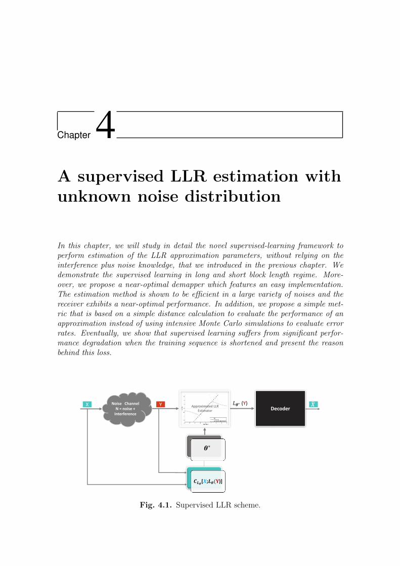
Chapter 4A supervised LLR estimation withunknown noise distribution
In this chapter, we will study in detail the novel supervised-learning framework toperform estimation of the LLR approximation parameters, without relying on theinterference plus noise knowledge, that we introduced in the previous chapter. Wedemonstrate the supervised learning in long and short block length regime. More-over, we propose a near-optimal demapper which features an easy implementation.The estimation method is shown to be efficient in a large variety of noises and thereceiver exhibits a near-optimal performance. In addition, we propose a simple met-ric that is based on a simple distance calculation to evaluate the performance of anapproximation instead of using intensive Monte Carlo simulations to evaluate errorrates. Eventually, we show that supervised learning suffers from significant perfor-mance degradation when the training sequence is shortened and present the reasonbehind this loss.
𝜽∗
𝑪𝑳𝜽[𝑿;𝑳𝜽(𝐘)]
Noise Channel N = noise +
Interference
YX 𝑿Decoder
Approximated LLR Estimator
𝐿𝜽∗ (Y)
Fig. 4.1. Supervised LLR scheme.

4.1. Supervised scheme 62
4.1 Supervised scheme
If the optimization of the criterion HK(X|Y ) (3.18) is performed in a supervisedmanner, the value of the parameter θ∗ is triggered after receiving the channel
output Y as shown in Figure 4.1. As we rely on Monte Carlo calculation to estimate(3.18), we need a known sequence of channel inputs, thanks to the learning sequencex1, . . . , xK and the corresponding outputs y1, . . . , yK . Once the optimal parameter θ∗
is obtained over the designed channel, it is used to build the approximated demapperfor the rest of the block as Lθ∗(Y ).
We investigate the accuracy of the supervised process with long block lengthperformance analysis in Section 4.2, thereafter, we study the effect of shorteningthe training sequence in Section 4.3. For clarity reasons we first focus on SαS noisedistributions, while we extend to other noise models with high and low impulsivecases, in particular, Middleton, ε−contaminated and Gaussian to investigate therobustness and the ability to adapt to different contexts. In order to assess theoptimal performance of the supervised approach, we use a large learning sequenceof 20000 samples to estimate a and b. This allows having a good grasp of the resultswith high estimation accuracy. To evaluate the performance of the proposed schemewe will use Lab (3.10) and present the BER curves using LDPC codes.
4.2 Supervised learning with long block length
regime
In this section, we investigate the accuracy of the supervised parameters estimation.
4.2.1 Parameter estimation performance analysis
The performance of the estimation process is evaluated over different noise models.To perform so, we compare the LLR shape obtained by the tuned θ∗ with the trueLLR. In order to be efficient, we can expect that the approximated demapper Lab isclose to the true one.
Estimation over impulsive SαS additive noise
Figure 4.2 and Figure 4.3 illustrates the LLR behavior of a SαS channel output forfixed value of α and by varying γ. First note, we can see that in all cases linear andasymptotic regions appear, as described in Section 3.2.4. Second, for each channelstate realization depicted by the couple α, γ, different LLR shapes are observed,thus, to match the channel state it is important to estimate correctly the LLRparameters. Third, by comparing the asymptotic part behavior between Figure 4.3and Figure 4.2 we can see that as the environment becomes more impulsive (bydecreasing α) the LLR asymptotic part will be almost the same in spite of varyingγ. Consequently, we can expect that the LLR approximation in high impulsiveenvironments will be less sensitive to parameters’ variations.
Figure 4.4 compares the evolution of the mean of the estimated parameters a andb, as a function of the dispersion γ of a SαS noise with α = 1.4 for the supervised

63 CHAPTER 4. SUPERVISED ESTIMATION
Fig. 4.2. Behavior of the LLR according to the output of the SαS channel for afixed α = 1.8 and different values of γ.
Fig. 4.3. Behavior of the LLR according to the output of the SαS channel for afixed α = 1.4 and different values of γ.
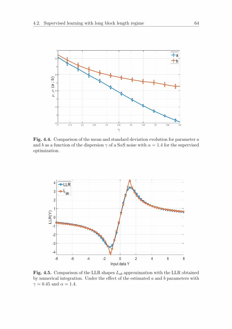
4.2. Supervised learning with long block length regime 64
Fig. 4.4. Comparison of the mean and standard deviation evolution for parameter aand b as a function of the dispersion γ of a SαS noise with α = 1.4 for the supervisedoptimization.
Fig. 4.5. Comparison of the LLR shapes Lab approximation with the LLR obtainedby numerical integration. Under the effect of the estimated a and b parameters withγ = 0.45 and α = 1.4.

65 CHAPTER 4. SUPERVISED ESTIMATION
Fig. 4.6. Comparison of the mean evolution for parameter a as a function of Eb/N0,under the Gaussian noise, the supervised optimization and the optimal receiver.
optimization. Remark that the same behaviors can be obtained for other values of αbetween 0 and 2. For each channel state, a and b are resultant of 5000 experiments.We notice that the variability in the estimated values is very small.
Figure 4.5 compares the LLR shapes of Lab obtained under supervised optimiza-tion with the true LLR obtained by numerical integration. For this comparisonwe select from Figure 4.4 γ = 0.45 (depicts the waterfall region) the estimated pa-rameters a = 3.6 and b = 5.1 that will be used to tune the Lab demapper. Thiscomparison shows the good fit between the approximated demapper Lab and thetrue LLR. Accordingly, we can expect a good BER performance.
Estimation over Gaussian noise
It is an essential feature that our proposal does not degrade the performance ofcommunication when no impulsiveness is present. Figure 4.6 compares the evolutionof the mean of the optimized parameter a and b obtained under the supervisedapproach to the optimal slope in the linear receiver aLLR. For each noise variance,we ran 5000 experiments. Recall that with our proposed demapper, the decreasingpart starts at ±
√b/a. If this value becomes large enough, the power-law part will
not impact the receiver. For Gaussian noise, large received samples are very rare,so that all samples fall into the linear part of the demapper. Numerically, whensimulating AWGN channel, we obtained values bigger than 49 for b as shown inFigure 4.6 which are larger than the one obtained for a, showing that only the linearpart impacts the receiver1. The decreasing part has consequently a negligible impact.The linear part is given by the optimal slope as a = 2/σ2. This comparison shows
1As Eb/N0 increases the noise standard deviation σ will decrease, making thus all the receivedsamples well-framed around the mean, that is the amplitude are mostly within 3σ of the mean.Consequently, all the received samples fall between ±
√b/a values and thus effected solely by the
linear part.

4.2. Supervised learning with long block length regime 66
𝜸 = 𝟎. 𝟑𝟓 𝜸 = 𝟎. 𝟒𝟓 𝜸 = 𝟎. 𝟓𝟓
Fig. 4.7. Behavior study of the HK function, as a function of parameters a and bfor different values of γ, under highly impulsive SαS noise with α = 1.4.
clearly the good fit between the slopes, proving thus the strength of the supervisedoptimization of the demapping function Lab over the AWGN channel.
4.2.2 Performance evaluation
Indirect link between the optimization method and minimizing BER
In a first step, we investigate the shape of the function HK (3.18) according toθ = (a, b). We present the obtained results for a highly impulsive noise when α = 1.4,but similar observations and conclusions would be made for other choices.
In Figure 4.7, we represent a 3D plot of the function HK for three values of γ,namely γ = 0.35, γ = 0.45 and γ = 0.55, representing the levels of HK under thesupervised criterion using a learning sequence of length 20000. The white contourin the middle figure delineates the area where the HK is less than 0.3 and this valuedecreases as γ decrease. The values of γ are selected in a way to represent the shapeof the function HK before, within and after the waterfall region, respectively, as willbe seen later in Section 4.2.1. First note that HK is quite flat around its minimumvalue. As a consequence, it may be quite sensitive to noise and thus to the lengthof the training sequence.
In Figure 4.8, we illustrate the link between the function HK and the obtainedBER. The contour plot delineates different BER values, ranging from 10−5 to 10−1,whereas the white contour delineates the set of a and b values yielding the smallestvalues of HK as shown in the middle figure of Figure 4.7. Note that the regionsmatch in the sense that the set of optimal values for a and b allows the decoder toachieve a BER below 10−5.
Indeed, as shown in Figure 4.8 when γ = 0.45, both a and b estimated meanvalues under the supervised optimization shown in Figure 4.4 fall in the small BERregion. Besides, the small variance of the estimated θ∗ ensures that the estimated

67 CHAPTER 4. SUPERVISED ESTIMATION
10−5
10−4
10−3
10−2
10−1
𝟏𝟎−𝟓𝟏𝟎−𝟒
𝟏𝟎−𝟑
𝟏𝟎−𝟐
BER
Fig. 4.8. BER comparison as a function of a and b parameters with γ = 0.45 andα = 1.4 under the supervised approximation.
values will fall in the region yielding the smallest BER.
The sensitivity to errors due to the flatness of the landscape of HK is thuslessened by the flatness of the BER region.
BER performance under SαS noise
Once our demapper is tuned with the estimated value θ∗, it is used as a front-endto the 20000 bits long regular (3,6) LDPC decoder using the BP algorithm. We testthis scheme first over an additive impulsive SαS noise.
In this case, we study a highly impulsive situation with α = 1.4 and a lessimpulsive case with α = 1.8. Figure 4.9 and Figure 4.10 present the BER forα = 1.4 and α = 1.8 respectively, as a function of the dispersion γ of the α-stablenoise2. In both cases, we compare the BER obtained via the demapping functionin a supervised manner, to the BER obtained with the true LLR computed vianumerical integration.
First, we note that in both cases, the estimation with such a long training se-quence gives performance close to the optimal LLR which shows the good behaviorof our solution. Secondly, we can figure out the ability to adapt to different impulsivestates from low impulsive up to highly impulsive.
In order to stress the need of good LLR shape design, we also optimized withour solution a linear approximation La. This receiver shows very poor performancebehavior in all impulsive cases. Thus, the impulsive nature must be tackled with adecreasing part of the LLR approximation such as with Lab.
2Recall that in case of an impulsive environment with α < 2, the second-order moment of astable variable is infinite [BSF08, Theorem 3], making the conventional noise power measurementinfinite. Accordingly, we present our simulation results as a function of the dispersion parameterγ, which is used as a measurement of the strength of the α-stable noise.

4.2. Supervised learning with long block length regime 68
Fig. 4.9. Evolution comparison of the BER as a function of the dispersion γ ofa SαS noise in low impulsive environment with α = 1.8, between the supervised,linear LLR approximations and the LLR obtained by numerical integration.
Fig. 4.10. Evolution comparison of the BER as a function of the dispersion γ ofa SαS noise in highly impulsive environment with α = 1.4, between the supervised,linear LLR approximations and the LLR obtained by numerical integration.
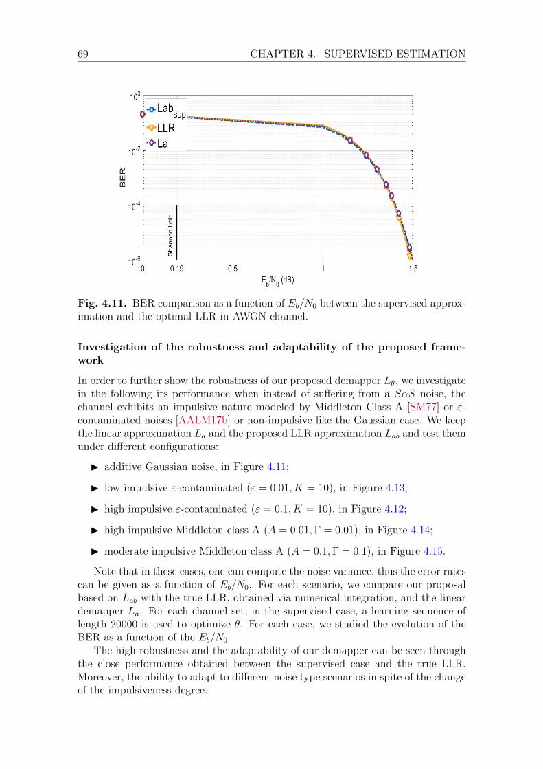
69 CHAPTER 4. SUPERVISED ESTIMATION
Fig. 4.11. BER comparison as a function of Eb/N0 between the supervised approx-imation and the optimal LLR in AWGN channel.
Investigation of the robustness and adaptability of the proposed frame-work
In order to further show the robustness of our proposed demapper Lθ, we investigatein the following its performance when instead of suffering from a SαS noise, thechannel exhibits an impulsive nature modeled by Middleton Class A [SM77] or ε-contaminated noises [AALM17b] or non-impulsive like the Gaussian case. We keepthe linear approximation La and the proposed LLR approximation Lab and test themunder different configurations:
I additive Gaussian noise, in Figure 4.11;
I low impulsive ε-contaminated (ε = 0.01, K = 10), in Figure 4.13;
I high impulsive ε-contaminated (ε = 0.1, K = 10), in Figure 4.12;
I high impulsive Middleton class A (A = 0.01,Γ = 0.01), in Figure 4.14;
I moderate impulsive Middleton class A (A = 0.1,Γ = 0.1), in Figure 4.15.
Note that in these cases, one can compute the noise variance, thus the error ratescan be given as a function of Eb/N0. For each scenario, we compare our proposalbased on Lab with the true LLR, obtained via numerical integration, and the lineardemapper La. For each channel set, in the supervised case, a learning sequence oflength 20000 is used to optimize θ. For each case, we studied the evolution of theBER as a function of the Eb/N0.
The high robustness and the adaptability of our demapper can be seen throughthe close performance obtained between the supervised case and the true LLR.Moreover, the ability to adapt to different noise type scenarios in spite of the changeof the impulsiveness degree.
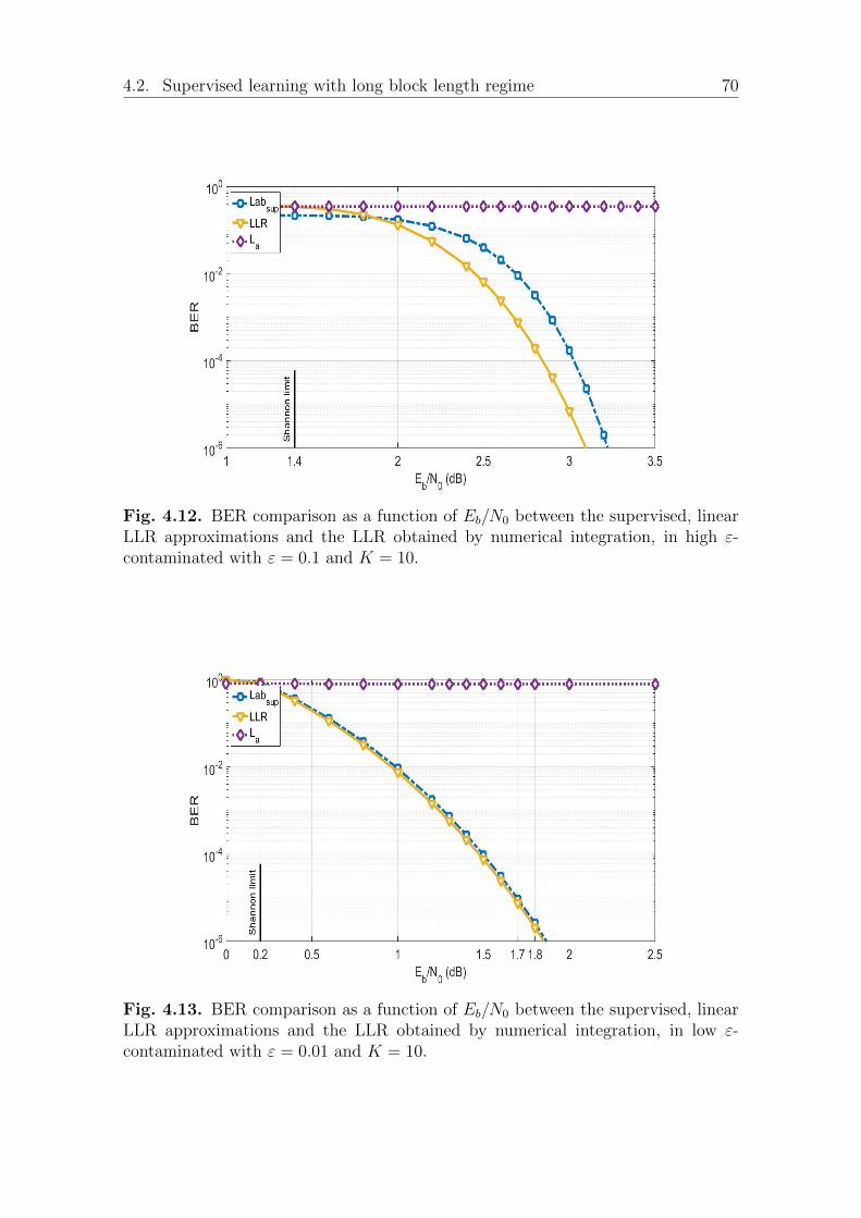
4.2. Supervised learning with long block length regime 70
Fig. 4.12. BER comparison as a function of Eb/N0 between the supervised, linearLLR approximations and the LLR obtained by numerical integration, in high ε-contaminated with ε = 0.1 and K = 10.
Fig. 4.13. BER comparison as a function of Eb/N0 between the supervised, linearLLR approximations and the LLR obtained by numerical integration, in low ε-contaminated with ε = 0.01 and K = 10.
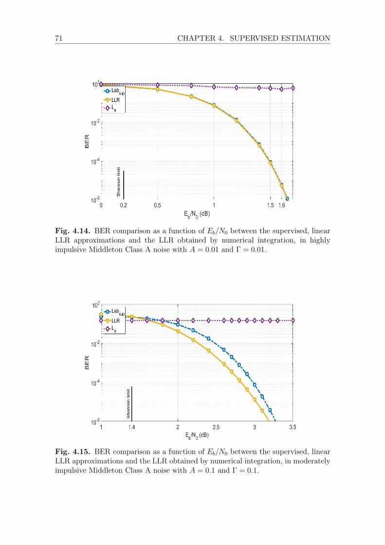
71 CHAPTER 4. SUPERVISED ESTIMATION
Fig. 4.14. BER comparison as a function of Eb/N0 between the supervised, linearLLR approximations and the LLR obtained by numerical integration, in highlyimpulsive Middleton Class A noise with A = 0.01 and Γ = 0.01.
Fig. 4.15. BER comparison as a function of Eb/N0 between the supervised, linearLLR approximations and the LLR obtained by numerical integration, in moderatelyimpulsive Middleton Class A noise with A = 0.1 and Γ = 0.1.
4.2. Supervised learning with long block length regime 72
Analysis and discussion: these numerical simulations illustrate the universalityof the supervised approach framework. The LLR family has to be wide enough toencompass the linear behavior of exponential-tail noises like the Gaussian and thenon-linear behavior of sub-exponential distributions of the impulsive noises. Theestimation of the LLR approximation parameter relies on an information theorycriteria that does not depend on any noise assumption. Consequently, this allowsour supervised framework to adapt to different noise models with different impulsivedegrees.
The gap between the supervised optimization and the true LLR is small in all thestudied examples. We extended this study to other noises parameters or a mixtureof distributions, for instance, the Gaussian plus stable noise and obtained similarconclusions. In impulsive situations, the gap between the non-linear LLR approx-imation Lθ and the linear receiver La is huge. It proves the influence of handlingcorrectly the impulses that arise due to the presence of interference. Moreover, ourdemapper function does not impact the performance when noise is not impulsive sothat we do not need a detection step to distinguish between Gaussian and impulsivesituations.
In the aforementioned study, we used a long learning sequence of 20000 samplesto estimate a and b. Consequently, the performance of the decoder depends onlyon the quality of the LLR approximation and not on estimation errors. Thus, theexisting gap compared to the true LLR in the BER figures especially when theimpulsiveness increases is relevant to the approximated LLR by itself. In the sake ofcompleteness, we deal with this loss by proposing in the next section a new demapperwith an added parameter which allows to significantly reduce the gap.
4.2.3 A robust and simple LLR approximation for receiverdesign
Note that the approximated LLR receiver Lab will remain one reference as it gives thebest performance compared to other proposed approximations [HLZ14], [MJLC15].
The main problem behind Lab is the rough transition between the linear partand the asymptotic part, where one can note, see Figure 4.16, a large gap betweenthe true LLR and the approximated one. The purple curve (or dots) denoted by thePDF of the received samples, represents the conditional probabilities Pr(Y |X = +1),respectively Pr(Y |X = −1). One can note that a large proportion of the receivedsamples fall in the transition part, where the gap to the true LLR is the largest.Consequently, we propose a new approximation as represented in Figure 4.16. Thethird parameter corresponds to a saturation of the approximated LLR in the tran-sition part, allowing to decrease the gap to the true LLR. This new approximationis detailed in the following.
Proposed Approximation
We call the new demapper Labc. It decomposes the LLR into three regions:
I First, when the channel output y is small the linear approximation of the LLR

73 CHAPTER 4. SUPERVISED ESTIMATION
Fig. 4.16. Comparison of the LLR shapes under the effect of the estimated a andb parameters with γ = 0.45 and α = 1.4, in the Lab and Labc approximations withthe LLR obtained by numerical integration.
around zero is given by:
LLR(y) = logf(y − 1)
f(y + 1)
= logf(−1) + f ′(−1)y +O(y2)
f(1) + f ′(1)y +O(y2)
= −2f ′(1)
f(1)y +O(y3) ≈ ay.
(4.1)
I Second, using Proposition 2, a simple asymptotic expansion may well approx-imate the probability density function fα of stable variables with unitary scaleparameter [NS95],
fα(y) =n∑k=1
bk|y|αk+1
+O(|y|−α(n+1)−1
). (4.2)
Using such asymptotic expansion of α-stable distribution provides a very sim-ple LLR approximation based on the first term fα(y) ∝ |y|−(α+1) for largevalues of the channel output y,
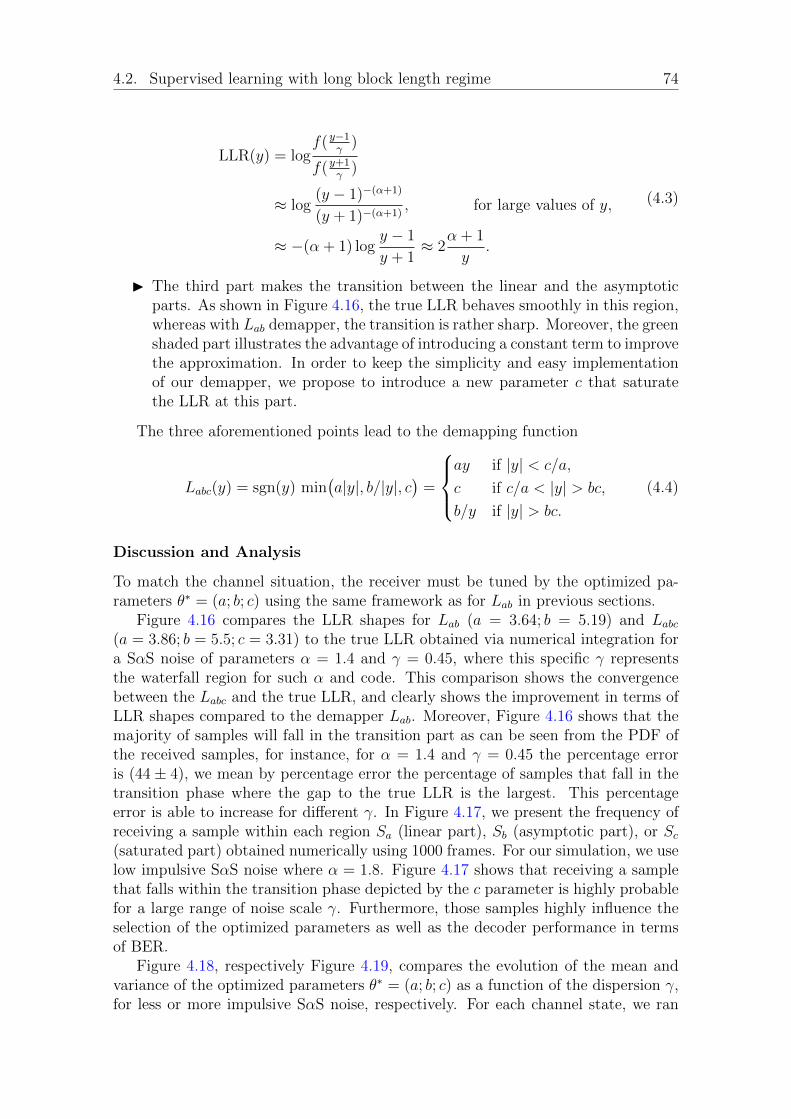
4.2. Supervised learning with long block length regime 74
LLR(y) = logf(y−1
γ)
f(y+1γ
)
≈ log(y − 1)−(α+1)
(y + 1)−(α+1), for large values of y,
≈ −(α + 1) logy − 1
y + 1≈ 2
α + 1
y.
(4.3)
I The third part makes the transition between the linear and the asymptoticparts. As shown in Figure 4.16, the true LLR behaves smoothly in this region,whereas with Lab demapper, the transition is rather sharp. Moreover, the greenshaded part illustrates the advantage of introducing a constant term to improvethe approximation. In order to keep the simplicity and easy implementationof our demapper, we propose to introduce a new parameter c that saturatethe LLR at this part.
The three aforementioned points lead to the demapping function
Labc(y) = sgn(y) min(a|y|, b/|y|, c
)=
ay if |y| < c/a,
c if c/a < |y| > bc,
b/y if |y| > bc.
(4.4)
Discussion and Analysis
To match the channel situation, the receiver must be tuned by the optimized pa-rameters θ∗ = (a; b; c) using the same framework as for Lab in previous sections.
Figure 4.16 compares the LLR shapes for Lab (a = 3.64; b = 5.19) and Labc(a = 3.86; b = 5.5; c = 3.31) to the true LLR obtained via numerical integration fora SαS noise of parameters α = 1.4 and γ = 0.45, where this specific γ representsthe waterfall region for such α and code. This comparison shows the convergencebetween the Labc and the true LLR, and clearly shows the improvement in terms ofLLR shapes compared to the demapper Lab. Moreover, Figure 4.16 shows that themajority of samples will fall in the transition part as can be seen from the PDF ofthe received samples, for instance, for α = 1.4 and γ = 0.45 the percentage erroris (44± 4), we mean by percentage error the percentage of samples that fall in thetransition phase where the gap to the true LLR is the largest. This percentageerror is able to increase for different γ. In Figure 4.17, we present the frequency ofreceiving a sample within each region Sa (linear part), Sb (asymptotic part), or Sc(saturated part) obtained numerically using 1000 frames. For our simulation, we uselow impulsive SαS noise where α = 1.8. Figure 4.17 shows that receiving a samplethat falls within the transition phase depicted by the c parameter is highly probablefor a large range of noise scale γ. Furthermore, those samples highly influence theselection of the optimized parameters as well as the decoder performance in termsof BER.
Figure 4.18, respectively Figure 4.19, compares the evolution of the mean andvariance of the optimized parameters θ∗ = (a; b; c) as a function of the dispersion γ,for less or more impulsive SαS noise, respectively. For each channel state, we ran

75 CHAPTER 4. SUPERVISED ESTIMATION
Fig. 4.17. Comparison of the mean evolution of the probability to fall within thea; b and c regions, as a function of the dispersion γ of a SαS noise with α = 1.8 forthe Labc.
Fig. 4.18. Comparison of the mean and standard deviation evolution for parametera; b and c as a function of the dispersion γ of a SαS noise with α = 1.8 for thedemapper Labc.
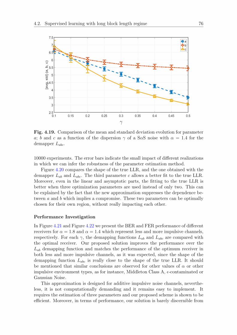
4.2. Supervised learning with long block length regime 76
Fig. 4.19. Comparison of the mean and standard deviation evolution for parametera; b and c as a function of the dispersion γ of a SαS noise with α = 1.4 for thedemapper Labc.
10000 experiments. The error bars indicate the small impact of different realizationsin which we can infer the robustness of the parameter estimation method.
Figure 4.20 compares the shape of the true LLR, and the one obtained with thedemapper Lab and Labc. The third parameter c allows a better fit to the true LLR.Moreover, even in the linear and asymptotic parts, the fitting to the true LLR isbetter when three optimization parameters are used instead of only two. This canbe explained by the fact that the new approximation suppresses the dependence be-tween a and b which implies a compromise. These two parameters can be optimallychosen for their own region, without really impacting each other.
Performance Investigation
In Figure 4.21 and Figure 4.22 we present the BER and FER performance of differentreceivers for α = 1.8 and α = 1.4 which represent less and more impulsive channels,respectively. For each γ, the demapping functions Lab and Labc are compared withthe optimal receiver. Our proposed solution improves the performance over theLab demapping function and matches the performance of the optimum receiver inboth less and more impulsive channels, as it was expected, since the shape of thedemapping function Labc is really close to the shape of the true LLR. It shouldbe mentioned that similar conclusions are observed for other values of α or otherimpulsive environment types, as for instance, Middleton Class A, ε-contaminated orGaussian Noise.
This approximation is designed for additive impulsive noise channels, neverthe-less, it is not computationally demanding and it remains easy to implement. Itrequires the estimation of three parameters and our proposed scheme is shown to beefficient. Moreover, in terms of performance, our solution is barely discernible from
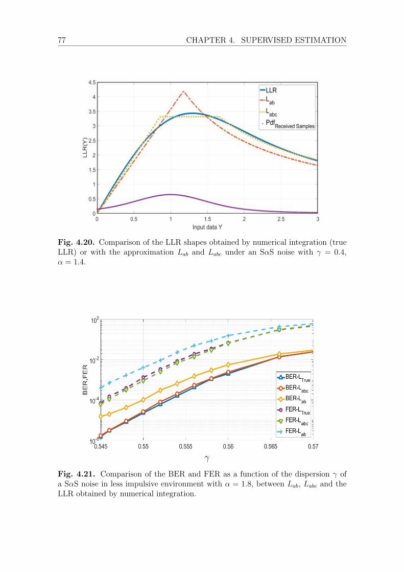
77 CHAPTER 4. SUPERVISED ESTIMATION
Fig. 4.20. Comparison of the LLR shapes obtained by numerical integration (trueLLR) or with the approximation Lab and Labc under an SαS noise with γ = 0.4,α = 1.4.
Fig. 4.21. Comparison of the BER and FER as a function of the dispersion γ ofa SαS noise in less impulsive environment with α = 1.8, between Lab, Labc and theLLR obtained by numerical integration.

4.3. Shortening the training sequence. 78
Fig. 4.22. Comparison of the BER and FER as a function of the dispersion γ of aSαS noise in highly impulsive environment with α = 1.4, between Lab, Labc and theLLR obtained by numerical integration.
the optimal receiver which is computationally prohibitive.
4.3 Shortening the training sequence.
So far we considered a learning sequence of the size of the LDPC code, which allowsto evaluate the LLR approximation without considering any performance impactinduced by the estimation step. However, in a practical setting, such a long trainingsequence is not reasonable and additional errors can be expected as the length ofthe learning sequence decreases.
In this section we will study the effect of the estimation when shortening thelearning sequence size.
We present in Table 4.1 the influence of the training sequence length. In thistable, the mean and the variance of the estimation of the parameters a and b arecollected for 20000, 1200 and 900 bits training sequences under moderate and lessimpulsive SαS noise with α = 1.4 and α = 1.8. The mean value of a is onlyslightly affected by the learning sequence length even for short or moderate lengthsequences. However, the standard deviation of the estimation significantly increases.On another hand, parameter b is more volatile and the mean of its estimation variessignificantly with the training sequence length. Such variability will affect the per-formance of the system and degrade the BER, asking for a trade-off between thetargeted BER and the sequence length.
Note that one can expect a performance degradation in terms of BER by project-ing the estimated values from Table 4.1 in Figure 4.7. Furthermore, in Figure 4.23we compare the LLR shapes of the Lab approximations obtained in the case of anα-stable noise with parameters α = 1.8 and γ = 0.55 for LS = 20000 and LS = 900

79 CHAPTER 4. SUPERVISED ESTIMATION
µa σa µb σb
α = 1.4
γ = 0.43SupLS=20000 3.73 0.07 5.10 0.12SupLS=1200 3.77 0.35 5.18 0.58SupLS=900 3.77 0.40 5.28 0.71
γ = 0.45SupLS=20000 3.57 0.07 5.06 0.13SupLS=1200 3.60 0.32 5.15 0.58SupLS=900 3.61 0.37 5.16 0.66
α = 1.8
γ = 0.53SupLS=20000 3.25 0.05 7.59 0.28SupLS=1200 3.27 0.24 8.50 14.48SupLS=900 3.27 0.27 11.72 46.15
γ = 0.55SupLS=20000 3.05 0.05 7.62 0.28SupLS=1200 3.07 0.22 7.97 1.54SupLS=900 3.07 0.26 10.73 30.41
Table 4.1 – Comparison of the mean and standard deviation evolution for the pa-rameters (a, b) as a function of the dispersion γ of a SαS noise with α = 1.4 andα = 1.8 for the supervised with different learning sequence sizes.
Fig. 4.23. Comparison of the Lab approximations obtained in the case α-stablenoise with parameters α = 1.8 and γ = 0.55 for different LS sizes with the TrueLLR obtained using numerical calculations.
with the true LLR using the mean of the estimated parameters in Table 4.1. Ob-viously, the LLR shape obtained by the estimated parameters of LS = 900 is farfrom the LLR shape. While the LLR shape obtained by the estimated parameters ofLS = 20000 is close to the true LLR shape. This degradation in the LLR shape willresult in a bad matching of the actual channel output Y and eventually a degraded

4.3. Shortening the training sequence. 80
Fig. 4.24. Showing the mismatch.
performance in terms of BER and FER.
We also (note even if it is counter-intuitive) that the estimated parameters aredegraded as α increases and γ decreases, in other words, when the channel becomesless impulsive. However, the intuitive way of thinking is that the more the channelbecomes impulsive the most difficult the estimation is, which is shown to be wrong.
In fact, when the channel becomes less impulsive the probability to observe rareevents (impulses) in the short training sequence (for instance LS=900) becomessmaller. However, this probability remains important in the whole message (20000).Thus, one can define a mismatch between what is learned from the LS and the realcondition of the whole message. To have a better understanding we demonstratethe existence of such a phenomenon in the following.
Mismatch between training phase and decoding phase: the estimation stepcan be tricky with impulsive noises because the most significant events are rare. Therisk is that what we learn from the learning sequence may not match the conditionof the message, leading to severe performance degradation.
Figure 4.24 shows three different impulsive states with SαS noise: less (α =1.8), medium (α = 1.4) and highly (α = 1.1) impulsive. The learning sequence(highlighted in the blue box) is chosen to be small (816 in our illustrative example).In each case, we compare the LS window to the up next 2000 received samples.
First, in Figure 4.24, α = 1.8 case, bottom plot, no impulse is observed in thetraining sequence and noise looks Gaussian. Consequently, the estimation will resultin a linear demapper which is perfect in such a case. However, some impulses withhigh amplitudes do appear outside the LS window. Due to the linear effect, theywill have a high likelihood and fool the receiver.
Second, in Figure 4.24, α = 1.4 case, few impulses fall in the LS window when
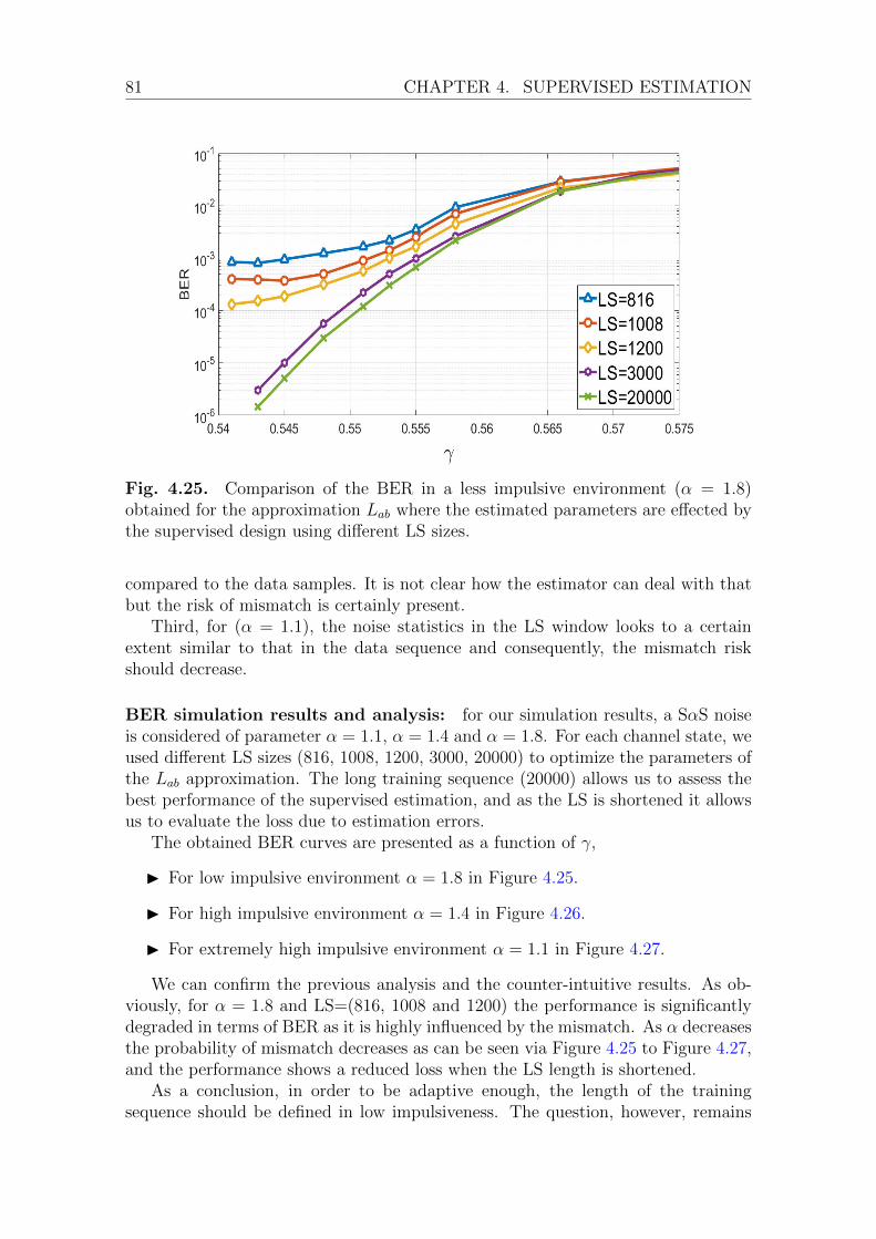
81 CHAPTER 4. SUPERVISED ESTIMATION
Fig. 4.25. Comparison of the BER in a less impulsive environment (α = 1.8)obtained for the approximation Lab where the estimated parameters are effected bythe supervised design using different LS sizes.
compared to the data samples. It is not clear how the estimator can deal with thatbut the risk of mismatch is certainly present.
Third, for (α = 1.1), the noise statistics in the LS window looks to a certainextent similar to that in the data sequence and consequently, the mismatch riskshould decrease.
BER simulation results and analysis: for our simulation results, a SαS noiseis considered of parameter α = 1.1, α = 1.4 and α = 1.8. For each channel state, weused different LS sizes (816, 1008, 1200, 3000, 20000) to optimize the parameters ofthe Lab approximation. The long training sequence (20000) allows us to assess thebest performance of the supervised estimation, and as the LS is shortened it allowsus to evaluate the loss due to estimation errors.
The obtained BER curves are presented as a function of γ,
I For low impulsive environment α = 1.8 in Figure 4.25.
I For high impulsive environment α = 1.4 in Figure 4.26.
I For extremely high impulsive environment α = 1.1 in Figure 4.27.
We can confirm the previous analysis and the counter-intuitive results. As ob-viously, for α = 1.8 and LS=(816, 1008 and 1200) the performance is significantlydegraded in terms of BER as it is highly influenced by the mismatch. As α decreasesthe probability of mismatch decreases as can be seen via Figure 4.25 to Figure 4.27,and the performance shows a reduced loss when the LS length is shortened.
As a conclusion, in order to be adaptive enough, the length of the trainingsequence should be defined in low impulsiveness. The question, however, remains
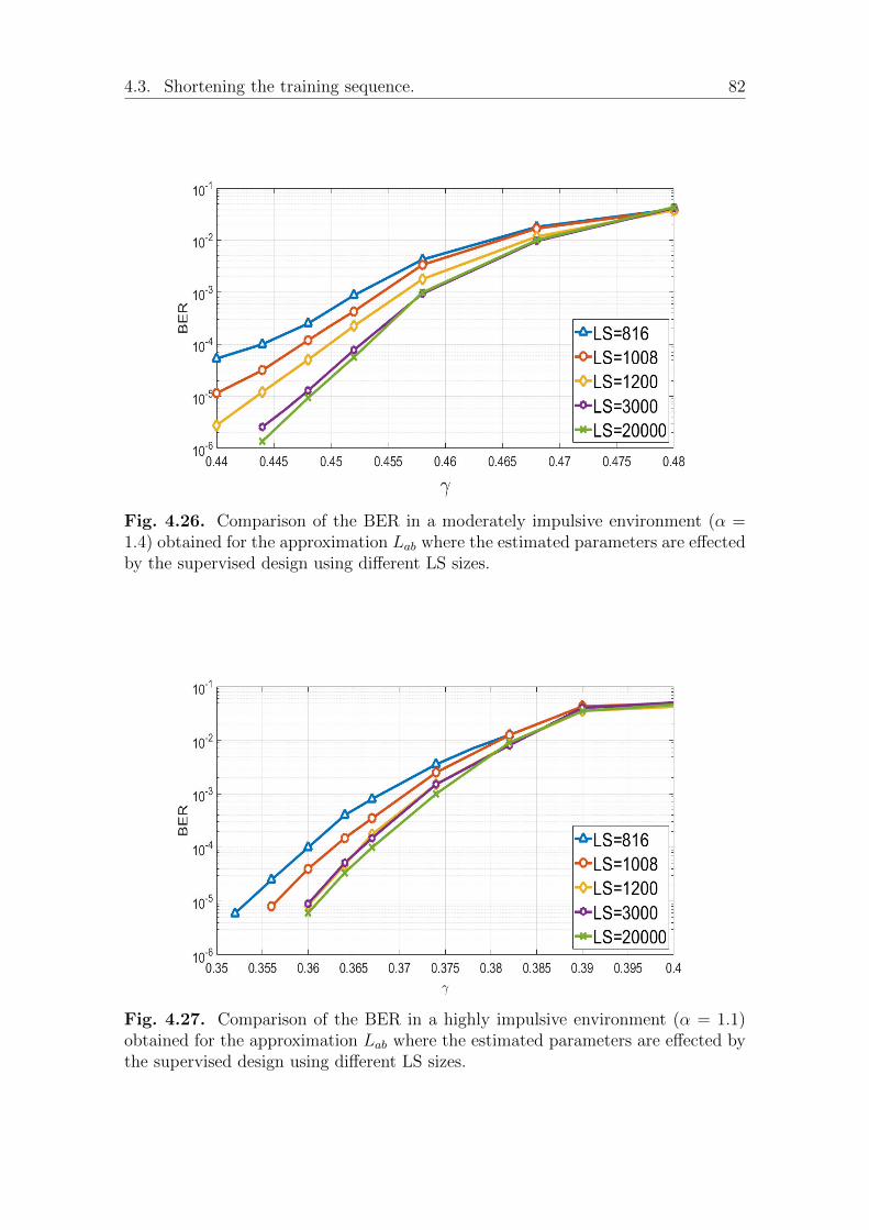
4.3. Shortening the training sequence. 82
Fig. 4.26. Comparison of the BER in a moderately impulsive environment (α =1.4) obtained for the approximation Lab where the estimated parameters are effectedby the supervised design using different LS sizes.
Fig. 4.27. Comparison of the BER in a highly impulsive environment (α = 1.1)obtained for the approximation Lab where the estimated parameters are effected bythe supervised design using different LS sizes.

83 CHAPTER 4. SUPERVISED ESTIMATION
complex and has also to account for the packet length. Quantifying the mismatchrisk in a simple way could be a solution to adjust the TS length.
But up to now we mainly rely on BER or FER to assess the performance ofthe system. Because we encompass a large number of noise models, analyticaltractability is complex to implement. We will in the next section introduce a metric,easier to handle than BER, to evaluate the performance of a LLR approximationfunction. This could be used in future work to design receivers and assess theirperformance in a more efficient way.
4.4 Indirect performance measurement of the LLR
approximations
In literature, different methods can be applied to evaluate the quality of differentapproximations (Lclip, Lab, ...) in a given channel. The most trivial method is thedirect exhaustive search using Monte Carlo simulation which can be done for variouschoices of LLR approximations for a given code. Then, the LLR approximationwhich gives rise to the best BER curve is chosen. However, this approach of findingthe best LLR approximation becomes rapidly too complex and long. In the previoussection and for estimation purposes, we used an indirect way of measuring the LLRfit with the capacity criterion (3.13). A capacity loss could be introduced to evaluatea LLR approximation.
Another way to measure the accuracy is the minimum mean square error (MMSE)between the true LLR and its approximation Lθ. In our study we consider threedifferent approximations, however, any approximation can fit the proposed frame-work. The three different approximations are: the clipping demapper Lclip(y) =
sgn(y) min(a|y|,
√ab); the approximated LLR Lab(y) = sgn(y) min
(a|y|, b/|y|
); our
previously proposed solution Labc(y) = sgn(y) min(a|y|, b/|y|, c
).
Figure 4.28 compares these different approximations and the true LLR obtainednumerically for an α-stable noise with α = 1.4 and a scale factor γ = 0.4. If theparameters are selected correctly, the simple functions Lclip, Lab and Labc are ratherclose to the LLR, at least in the linear region. In superimposition, the figure alsodisplays the density of the output Y knowing the input X; clearly, all regions of thevarious approximations are likely to be used.
The LLR approximation should be directly comparable to each other in orderto choose the best compromise between simplicity and performance. We propose touse the following criterion to rank the approximations
MSE =
∫ ∞−∞
[Λ(y)− Lθ(y)]2 p(y) dy = Ey [Λ(y)− Lθ(y)]2 . (4.5)
This metric is justified by the need for an approximation to get close to the truelikelihood of Λ(y). However, all regions must be weighted differently because thisapproximation must be better for the most likely y values, hence the p(y) factor.
More formally, it is possible to find two constants K and K ′ to frame the integral
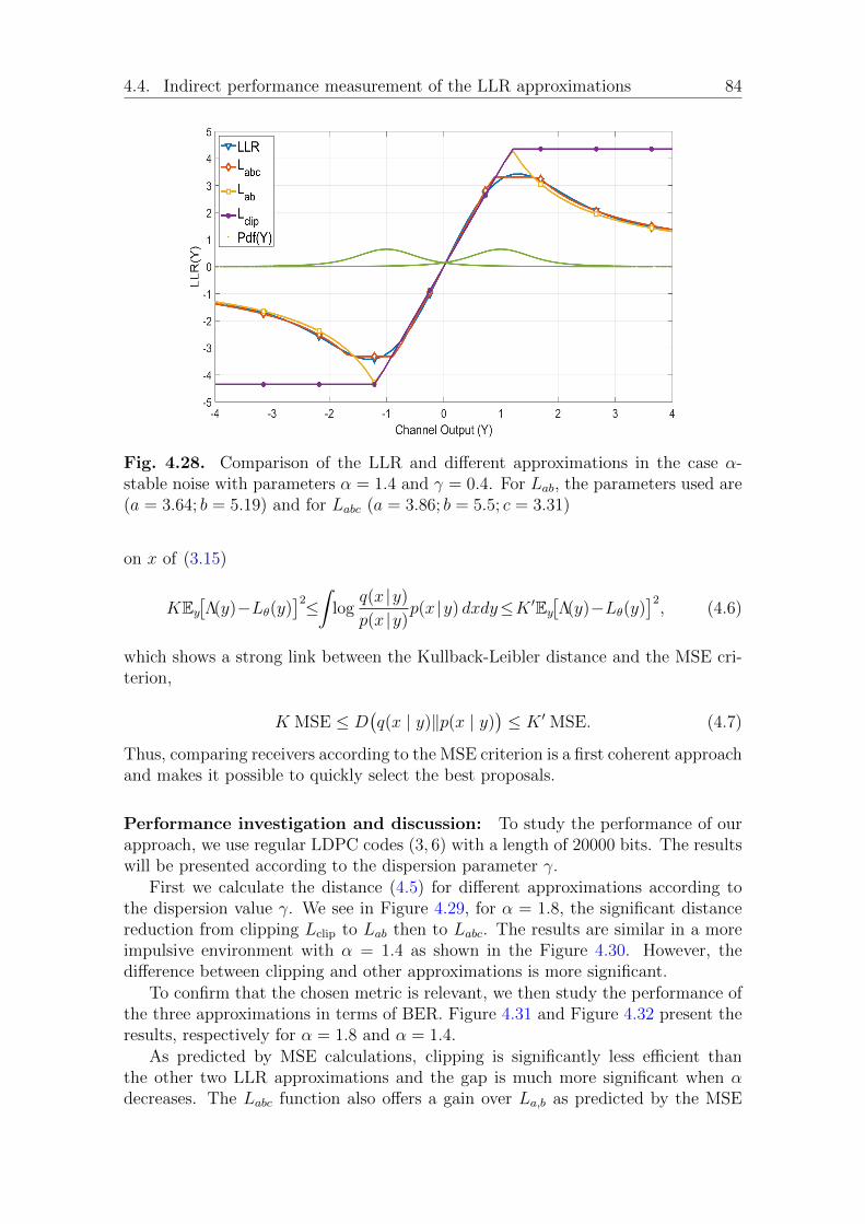
4.4. Indirect performance measurement of the LLR approximations 84
Fig. 4.28. Comparison of the LLR and different approximations in the case α-stable noise with parameters α = 1.4 and γ = 0.4. For Lab, the parameters used are(a = 3.64; b = 5.19) and for Labc (a = 3.86; b = 5.5; c = 3.31)
on x of (3.15)
KEy[Λ(y)−Lθ(y)
]2≤∫ logq(x |y)
p(x |y)p(x |y) dxdy≤K ′Ey
[Λ(y)−Lθ(y)
]2, (4.6)
which shows a strong link between the Kullback-Leibler distance and the MSE cri-terion,
K MSE ≤ D(q(x | y)‖p(x | y)
)≤ K ′ MSE. (4.7)
Thus, comparing receivers according to the MSE criterion is a first coherent approachand makes it possible to quickly select the best proposals.
Performance investigation and discussion: To study the performance of ourapproach, we use regular LDPC codes (3, 6) with a length of 20000 bits. The resultswill be presented according to the dispersion parameter γ.
First we calculate the distance (4.5) for different approximations according tothe dispersion value γ. We see in Figure 4.29, for α = 1.8, the significant distancereduction from clipping Lclip to Lab then to Labc. The results are similar in a moreimpulsive environment with α = 1.4 as shown in the Figure 4.30. However, thedifference between clipping and other approximations is more significant.
To confirm that the chosen metric is relevant, we then study the performance ofthe three approximations in terms of BER. Figure 4.31 and Figure 4.32 present theresults, respectively for α = 1.8 and α = 1.4.
As predicted by MSE calculations, clipping is significantly less efficient thanthe other two LLR approximations and the gap is much more significant when αdecreases. The Labc function also offers a gain over La,b as predicted by the MSE
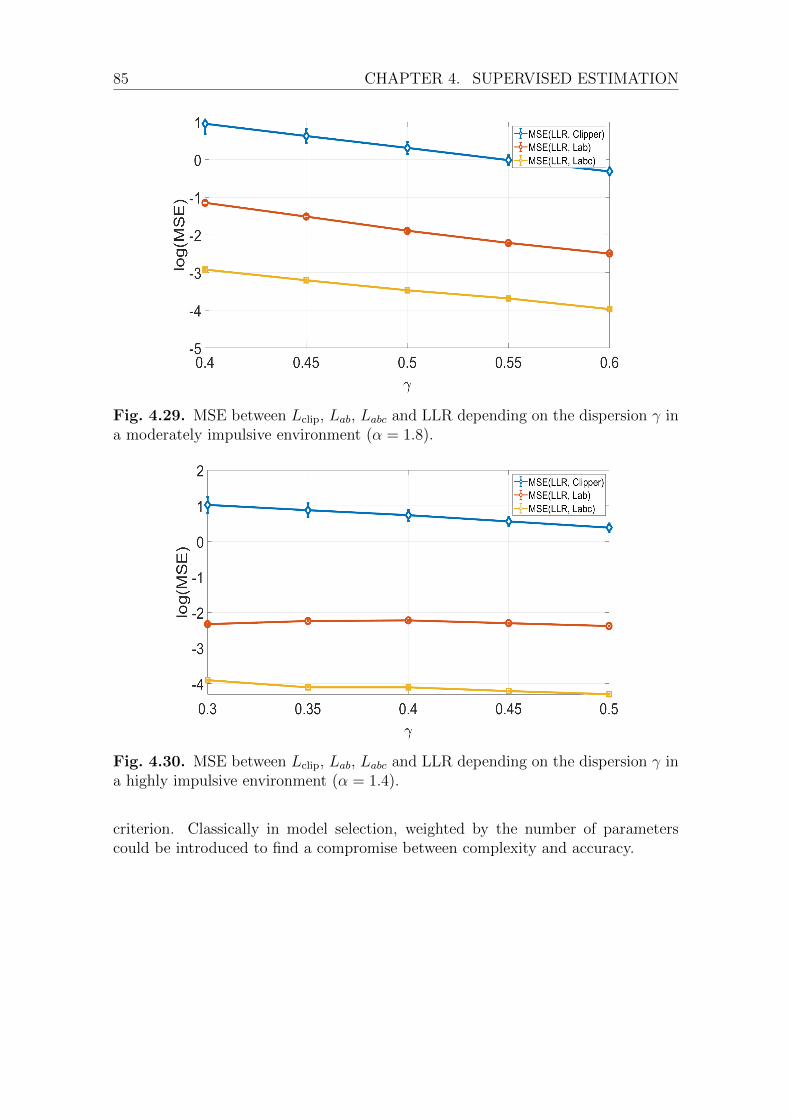
85 CHAPTER 4. SUPERVISED ESTIMATION
Fig. 4.29. MSE between Lclip, Lab, Labc and LLR depending on the dispersion γ ina moderately impulsive environment (α = 1.8).
Fig. 4.30. MSE between Lclip, Lab, Labc and LLR depending on the dispersion γ ina highly impulsive environment (α = 1.4).
criterion. Classically in model selection, weighted by the number of parameterscould be introduced to find a compromise between complexity and accuracy.
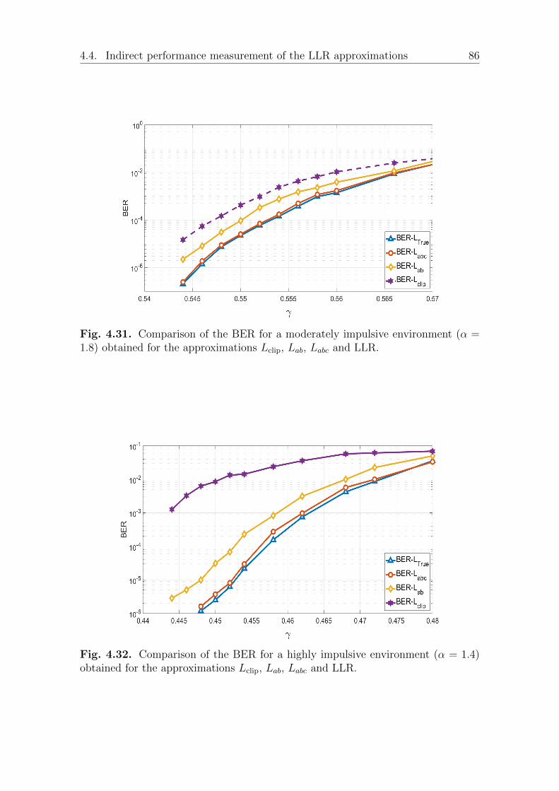
4.4. Indirect performance measurement of the LLR approximations 86
Fig. 4.31. Comparison of the BER for a moderately impulsive environment (α =1.8) obtained for the approximations Lclip, Lab, Labc and LLR.
Fig. 4.32. Comparison of the BER for a highly impulsive environment (α = 1.4)obtained for the approximations Lclip, Lab, Labc and LLR.

87 CHAPTER 4. SUPERVISED ESTIMATION
4.5 conclusion
The presence of interference or impulsive noise makes it difficult to calculate theLLRs required for decoding. We proposed in this chapter a flexible receiver designbased on a LLR approximation function fθ in a parametric family. The parameterθ is estimated through the maximization of the mutual information between thechannel input and the demapping of the channel output. A supervised estimationis proposed where first we test our framework using long sequence size. Our resultsshow that the supervised receiver design is efficient and robust in a large variety ofnoises and allows to reach performance close to the optimal.
In addition, we proposed a new LLR demapper based on a parameterized ap-proximation function with three optimization parameters. Numerical simulationsshow that the performance achieved match the one obtained with the true LLR.
Furthermore, to evaluate the performance of an approximation, we show that itis not necessary to use intensive Monte Carlo simulations but that a simple distancecalculation gives a precise idea of its performance. This makes it possible to workon the quality of the approximations and their adaptability to various contexts.Consequently, we evaluate the quality of the approximation by a mean squarederror and ascertain that this criterion is sufficient to identify the approximationsthat will be efficient.
All the obtained performances are investigated in a first approach by the useof a training sequence of the size of the codeword, in other words, assuming avery accurate estimation of the channel state. This is not realistic in real settings,for such, we evaluated the impact of shortening the training sequence. The task isespecially difficult with impulsive noise that makes the estimation step more complexand requires longer training sequence to observe enough rare events. In such acase, a risk of mismatch arises: the risk that what we learned from the learningsequence may not match the condition of the message, leading to severe performancedegradation. Indeed, the learning sequence has to be long enough to guarantee thepresence of the expected rare events. If this is not ensured, the estimation of θ won’tlead to a good LLR estimation.
A major drawback of the supervised approach relies on the necessity of thelearning sequence. As a consequence, it induces an increase in signaling and adecrease in the useful rate. Moreover, we show the LS has to be quite long toavoid the mismatch effect. For this reason, we propose in the following chapter anunsupervised estimation of θ, which focuses directly on the output of the channel,without any prior on the input.

4.5. conclusion 88

Chapter 5An unsupervised LLR estimationwith unknown noise distribution
In this chapter, we propose an unsupervised estimation of θ∗, avoiding the need of atraining sequence. The performance of our estimation method is first analyzed withlong codewords. It is shown to be efficient in a large variety of noises and the receiverexhibits a near-optimal performance. Next, this estimation is performed with shortcodewords, rending the estimation very error-sensitive. We analyze what conditionslead to the estimation failure, derive an analytical tool to assess the probability offailure and then propose to jointly use two mechanisms that prevent the aforemen-tioned failures. Our estimation is shown to be efficient and the receiver exhibits anear-optimal performance under various noisy environment types, ranging from veryimpulsive one to Gaussian.
5.1 Online parameter estimation and unsupervised
optimization
To ease the reading we recall that our optimization problem writes as:
θ∗=arg minθH(X|Y )=arg min
θE[log2
(1 + e−XLθ(Y )
)](5.1)
and can be solved using data samples as
θ∗ = arg minθ
1
K
K∑k=1
log2
(1 + e−xkLθ(yk)
), (5.2)
where K is the number of samples, xk and yk represent the input and the output ofthe channel, respectively. For more details see Section 3.5.1.
5.2 Unsupervised optimization
To solve (5.2), one needs a received sequence yk as well as the corresponding trans-mitted one xk. This is usually obtained thanks to the supervised approach where

5.2. Unsupervised optimization 90
θ∗
I[෩𝑿 ;𝑳θ(෩𝒀)]
Noise Channel N = noise +
Interference
𝐿θ∗ (Y)
෩𝑵
෩𝑿
Approximated LLR Demapper
Decoder
෩𝒀
Simulated Channel
𝑎∗ 𝑏∗
Fig. 5.1. Unsupervised LLR demapper scheme.
a training sequence is used as discusses in the previous chapter. However, this in-duces an increase in signaling and a decrease in the useful data rate. Unsupervisedoptimization is thus attractive since it does not imply any overload. Besides, a goodaspect of having such an unsupervised approach is that we optimize the approxi-mation function directly from the sequence that we are going to decode. In otherwords, the noise impacting the training phase and the decoding phase will be thesame ensuring the best knowledge of the actual channel state and the mismatchdiscussed in Section 4.3 becomes irrelevant.
Since one needs the sent sequence X as well as the corresponding channel outputY , we propose [MSG+19d,MSG+18] to extract a noise sequence N directly from thereceived channel output Y and to simulate at the receiver side the transmission ofa known sequence X. The corresponding channel output is build as Y = X + N , asdepicted in Figure 5.1. To do so, we propose to use a sign-detector yielding
N = Y − sign(Y ). (5.3)
The simulated channel input is an i.i.d. BPSK random variable, independent of N .Due to this independence, the input sequence can be chosen as a sequence of +1’s,so that the new channel output is Y = +1 + N . The optimization parameter θ canbe estimated based on (5.2) but with the newly generated input and output as
θ∗ = arg minθH(X|Y )
= arg minθ
1
K
K∑k=1
log2
(1 + e−xkLθ(yk)
)= arg min
θ
1
K
K∑k=1
log2
(1 + e−Lθ(yk)
),
(5.4)
where the last transition comes from the fact that we use X = +1. Once θ∗ isobtained, the LLR is approximated by Lθ∗(Y ), where Y is the true received sequenceover the MBISO channel.
In order to investigate the performance of the unsupervised approach, we aregoing to compare it in the following to the best achieved performance of the su-pervised approach (LS=20000). In the next section, we propose to apply our blind

91 CHAPTER 5. UNSUPERVISED ESTIMATION
LLR approximation optimization to LDPC coding where the noise exhibits eitherimpulsive or a Gaussian nature.
For our simulations, once our demapper is tuned with the estimated value θ∗,it is used as a front-end to the 20000 bits long regular (3,6) LDPC decoder whenlong block length regime analysis is considered and the 408 bits long regular (3,6)LDPC decoder when short block length regime analysis is considered using the BPalgorithm.
5.3 Unsupervised learning with long block length
regime
5.3.1 Parameter estimation
Estimation over impulsive SαS additive noise
In a first step, we compare the obtained θ∗ under blind optimization with the oneobtained under a supervised approach. In this section, we only present the obtainedresults for a highly impulsive noise when α = 1.4, but similar observations andconclusions can be made for other choices.
Figure 5.2, respectively 5.3, compares the evolution of the mean and varianceof the estimated parameter a, respectively b, as a function of the dispersion γ. Foreach noise dispersion, we ran 5000 experiments.
We can see from Figure 5.2 that the gap between the obtained values for pa-rameter a under supervised and unsupervised optimization keeps very small. Butunfortunately, as shown in Figure 5.3, the one obtained for b is significantly larger.This difference can be explained since b mainly depends on large noise samples whichare rare events; consequently, its estimation is more difficult.
In Figure 4.7, we represent a 3D plot of the function HK (5.2). We show that HK
is quite flat around its minimum value. As a consequence, it may be quite sensitiveto errors and thus to the length of the training sequence. Using the whole data setin an unsupervised approach can then be a source of robustness. We illustrate thelink between the function HK and the obtained BER. The contour plot delineatesdifferent BER values, ranging from 10−5 to 10−1.
In Figure 5.4, we project the two white crosses correspond to the mean value ofthe optimization parameters a and b obtained under supervised and unsupervisedoptimization, as provided on Figure 5.2 and Figure 5.3, respectively. Furthermore,the white contour delineates the set of a and b values yielding the smallest valuesof HK within a small precision error. First note that the obtained mean values ofa and b under both types of optimization fall within the set of points achieving aBER less than 10−5; the small variance of the estimated θ∗ under both cases ensuresthat most of the estimated values will fall in the region yielding the smallest BER.Thus, we can expect that the error on b will have a limited impact in terms ofBER performance. Through intensive simulations, we noticed that the connectionbetween HK and the BER is always assessed, irrespective of the noise model andnoise parameters value.
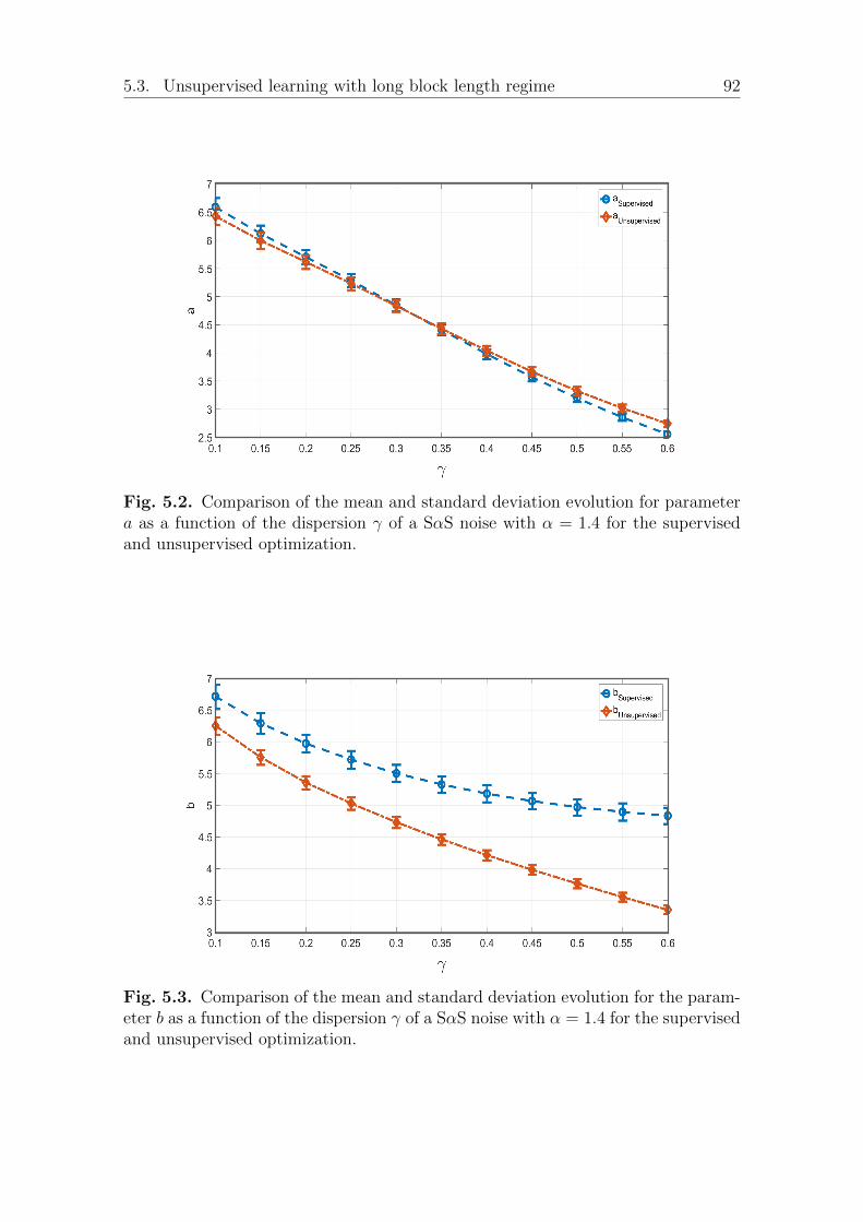
5.3. Unsupervised learning with long block length regime 92
Fig. 5.2. Comparison of the mean and standard deviation evolution for parametera as a function of the dispersion γ of a SαS noise with α = 1.4 for the supervisedand unsupervised optimization.
Fig. 5.3. Comparison of the mean and standard deviation evolution for the param-eter b as a function of the dispersion γ of a SαS noise with α = 1.4 for the supervisedand unsupervised optimization.

93 CHAPTER 5. UNSUPERVISED ESTIMATION
BER
10−5
10−4
10−3
10−2
10−1
Unsupervised
Supervised
𝟏𝟎−𝟑
𝟏𝟎- 𝟐
𝟏𝟎−𝟒
𝟏𝟎−𝟓
Fig. 5.4. BER comparison as a function of a and b parameters with γ = 0.45 andα = 1.4 under the supervised approximation.
µa σa µb σb
α = 1.8
γ = 0.53
Unsupervised 3.43 0.06 5.73 0.15SupLS=20000 3.25 0.05 7.59 0.28SupLS=1200 3.27 0.24 8.50 14.48SupLS=900 3.27 0.27 11.72 46.15
γ = 0.55
Unsupervised 3.23 0.05 5.61 0.14SupLS=20000 3.05 0.05 7.62 0.28SupLS=1200 3.07 0.22 7.97 1.54SupLS=900 3.07 0.26 10.73 30.41
Table 5.1 – Parameter Estimation. Comparison of the mean and standard deviationevolution for the parameters (a, b) as a function of the dispersion γ of a SαS noisewith α = 1.8 for the supervised with different learning sequences and unsupervisedoptimization.
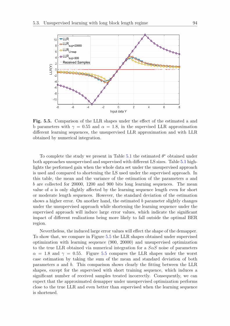
5.3. Unsupervised learning with long block length regime 94
Fig. 5.5. Comparison of the LLR shapes under the effect of the estimated a andb parameters with γ = 0.55 and α = 1.8, in the supervised LLR approximationdifferent learning sequences, the unsupervised LLR approximation and with LLRobtained by numerical integration.
To complete the study we present in Table 5.1 the estimated θ∗ obtained underboth approaches unsupervised and supervised with different LS sizes. Table 5.1 high-lights the performed gain when the whole data set under the unsupervised approachis used and compared to shortening the LS used under the supervised approach. Inthis table, the mean and the variance of the estimation of the parameters a andb are collected for 20000, 1200 and 900 bits long learning sequences. The meanvalue of a is only slightly affected by the learning sequence length even for shortor moderate length sequences. However, the standard deviation of the estimationshows a higher error. On another hand, the estimated b parameter slightly changesunder the unsupervised approach while shortening the learning sequence under thesupervised approach will induce large error values, which indicate the significantimpact of different realizations being more likely to fall outside the optimal BERregion.
Nevertheless, the induced large error values will effect the shape of the demapper.To show that, we compare in Figure 5.5 the LLR shapes obtained under supervisedoptimization with learning sequence (900, 20000) and unsupervised optimizationto the true LLR obtained via numerical integration for a SαS noise of parametersα = 1.8 and γ = 0.55. Figure 5.5 compares the LLR shapes under the worstcase estimation by taking the sum of the mean and standard deviation of bothparameters a and b. This comparison shows clearly the fitting between the LLRshapes, except for the supervised with short training sequence, which induces asignificant number of received samples treated incorrectly. Consequently, we canexpect that the approximated demapper under unsupervised optimization performsclose to the true LLR and even better than supervised when the learning sequenceis shortened.
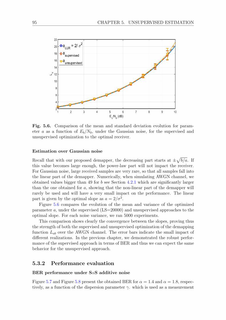
95 CHAPTER 5. UNSUPERVISED ESTIMATION
Fig. 5.6. Comparison of the mean and standard deviation evolution for param-eter a as a function of Eb/N0, under the Gaussian noise, for the supervised andunsupervised optimization to the optimal receiver.
Estimation over Gaussian noise
Recall that with our proposed demapper, the decreasing part starts at ±√b/a. If
this value becomes large enough, the power-law part will not impact the receiver.For Gaussian noise, large received samples are very rare, so that all samples fall intothe linear part of the demapper. Numerically, when simulating AWGN channel, weobtained values bigger than 49 for b see Section 4.2.1 which are significantly largerthan the one obtained for a, showing that the non-linear part of the demapper willrarely be used and will have a very small impact on the performance. The linearpart is given by the optimal slope as a = 2/σ2.
Figure 5.6 compares the evolution of the mean and variance of the optimizedparameter a, under the supervised (LS=20000) and unsupervised approaches to theoptimal slope. For each noise variance, we ran 5000 experiments.
This comparison shows clearly the convergence between the slopes, proving thusthe strength of both the supervised and unsupervised optimization of the demappingfunction Lab over the AWGN channel. The error bars indicate the small impact ofdifferent realizations. In the previous chapter, we demonstrated the robust perfor-mance of the supervised approach in terms of BER and thus we can expect the samebehavior for the unsupervised approach.
5.3.2 Performance evaluation
BER performance under SαS additive noise
Figure 5.7 and Figure 5.8 present the obtained BER for α = 1.4 and α = 1.8, respec-tively, as a function of the dispersion parameter γ. which is used as a measurement
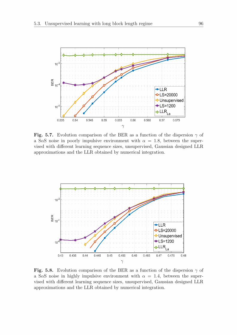
5.3. Unsupervised learning with long block length regime 96
Fig. 5.7. Evolution comparison of the BER as a function of the dispersion γ ofa SαS noise in poorly impulsive environment with α = 1.8, between the super-vised with different learning sequence sizes, unsupervised, Gaussian designed LLRapproximations and the LLR obtained by numerical integration.
Fig. 5.8. Evolution comparison of the BER as a function of the dispersion γ ofa SαS noise in highly impulsive environment with α = 1.4, between the super-vised with different learning sequence sizes, unsupervised, Gaussian designed LLRapproximations and the LLR obtained by numerical integration.

97 CHAPTER 5. UNSUPERVISED ESTIMATION
of the strength of the α-stable noise. In both cases, we compare the BER obtainedvia the demapping function Lab, either in an unsupervised or supervised manner,to the BER obtained with the true LLR computed via numerical integration. Foreach channel set, we use a learning sequence of length 1200 or 20000 samples tooptimize θ in the supervised case; the long training sequence (20000) allows to as-sess the optimal performance of the supervised estimation, the shorter one (1200)allows to evaluate the loss due to estimation with more realistic training sequences.The unsupervised approach does not perform as well as the supervised one witha long training sequence but the gap is restrained. However, in comparison to alinear receiver gain is huge. Moreover, when the training sequence is shortened, thesupervised estimation degrades and the performance of the unsupervised approachis then much better.
In order to show the robustness of our proposed unsupervised framework, we in-vestigate in the following its performance when the channel exhibits either an impul-sive nature modeled by: Middleton Class A [SM77] noise, ε-contaminated [AALM17b]noise or simply a Gaussian noise.
BER over Gaussian and other impulsive noises
The different configurations
I Gaussian noise in Figure 5.9
I high impulsive Middleton environment with A = 0.01 and Γ = 0.01 in Fig-ure 5.10
I moderate impulsive Middleton environment with A = 0.1 and Γ = 0.1 inFigure 5.11
I low impulsive ε−contaminated environment with ε = 0.01 and K = 10 inFigure 5.12.
I high impulsive ε−contaminated environment with ε = 0.1 and K = 10 inFigure 5.13.
For each scenario, we compare the true LLR, obtained via numerical integrationto the LLR approximations under supervised with 20000 long learning sequence,unsupervised parameter estimation and Gaussian designed demapper La.
In Figure 5.9 (Gaussian noise) all curves are almost superposed, with a smallperformance loss under the unsupervised optimization. Our proposed approach Lθdoes not degrade the decoding performance in a purely Gaussian case under theunsupervised estimation.
In Figure 5.10 to Figure 5.13, the high robustness and adaptability of our receivercan be seen through the close performance obtained between the unsupervised andsupervised case from one side, and between the approximations and the true LLRfrom the other side in spite of the change of the type of noise and the degree ofimpulsiveness in all scenarios.
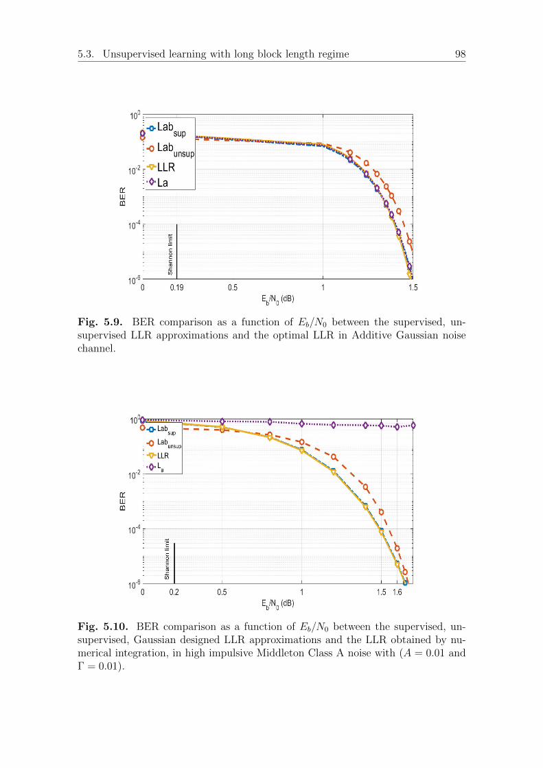
5.3. Unsupervised learning with long block length regime 98
Fig. 5.9. BER comparison as a function of Eb/N0 between the supervised, un-supervised LLR approximations and the optimal LLR in Additive Gaussian noisechannel.
Fig. 5.10. BER comparison as a function of Eb/N0 between the supervised, un-supervised, Gaussian designed LLR approximations and the LLR obtained by nu-merical integration, in high impulsive Middleton Class A noise with (A = 0.01 andΓ = 0.01).
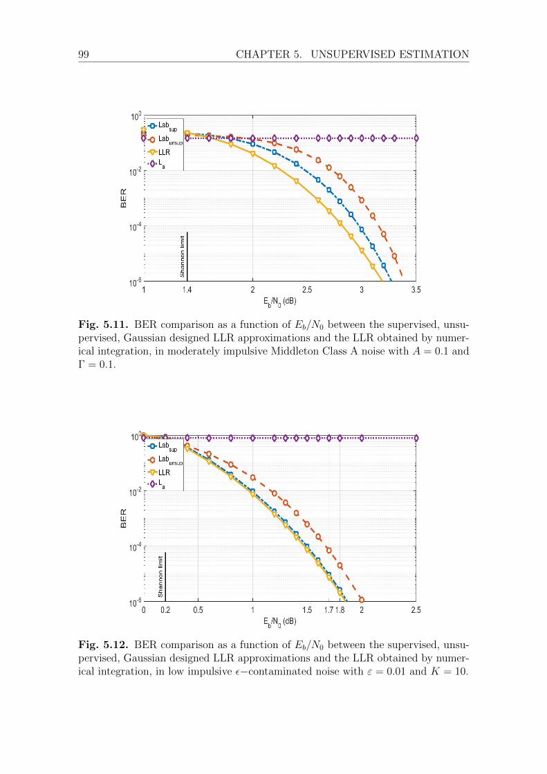
99 CHAPTER 5. UNSUPERVISED ESTIMATION
Fig. 5.11. BER comparison as a function of Eb/N0 between the supervised, unsu-pervised, Gaussian designed LLR approximations and the LLR obtained by numer-ical integration, in moderately impulsive Middleton Class A noise with A = 0.1 andΓ = 0.1.
Fig. 5.12. BER comparison as a function of Eb/N0 between the supervised, unsu-pervised, Gaussian designed LLR approximations and the LLR obtained by numer-ical integration, in low impulsive ε−contaminated noise with ε = 0.01 and K = 10.
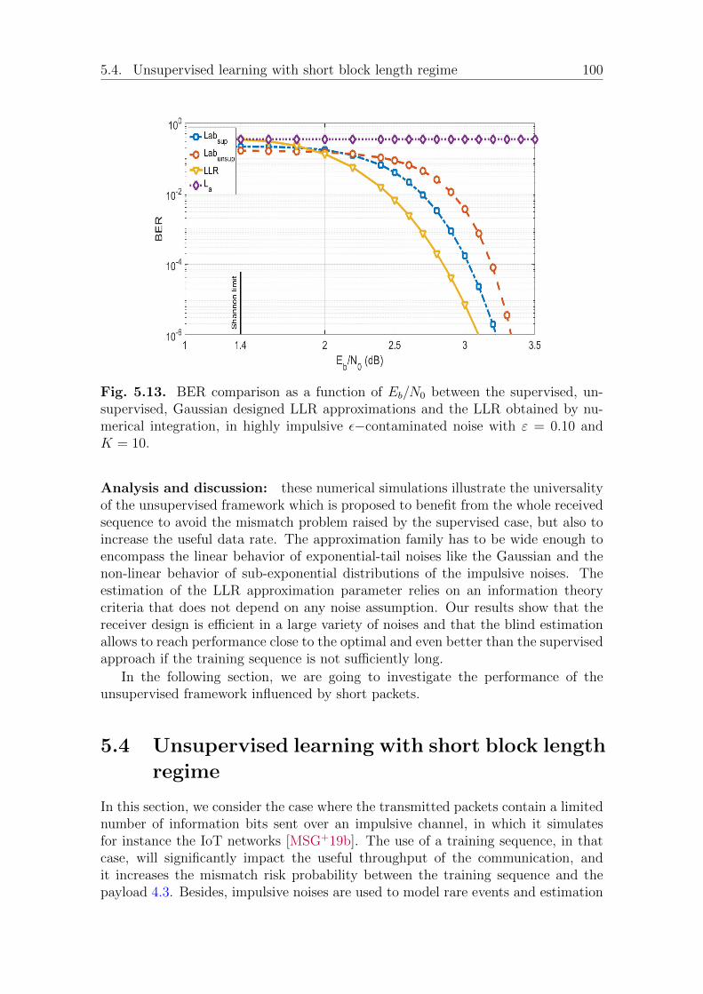
5.4. Unsupervised learning with short block length regime 100
Fig. 5.13. BER comparison as a function of Eb/N0 between the supervised, un-supervised, Gaussian designed LLR approximations and the LLR obtained by nu-merical integration, in highly impulsive ε−contaminated noise with ε = 0.10 andK = 10.
Analysis and discussion: these numerical simulations illustrate the universalityof the unsupervised framework which is proposed to benefit from the whole receivedsequence to avoid the mismatch problem raised by the supervised case, but also toincrease the useful data rate. The approximation family has to be wide enough toencompass the linear behavior of exponential-tail noises like the Gaussian and thenon-linear behavior of sub-exponential distributions of the impulsive noises. Theestimation of the LLR approximation parameter relies on an information theorycriteria that does not depend on any noise assumption. Our results show that thereceiver design is efficient in a large variety of noises and that the blind estimationallows to reach performance close to the optimal and even better than the supervisedapproach if the training sequence is not sufficiently long.
In the following section, we are going to investigate the performance of theunsupervised framework influenced by short packets.
5.4 Unsupervised learning with short block length
regime
In this section, we consider the case where the transmitted packets contain a limitednumber of information bits sent over an impulsive channel, in which it simulatesfor instance the IoT networks [MSG+19b]. The use of a training sequence, in thatcase, will significantly impact the useful throughput of the communication, andit increases the mismatch risk probability between the training sequence and thepayload 4.3. Besides, impulsive noises are used to model rare events and estimation
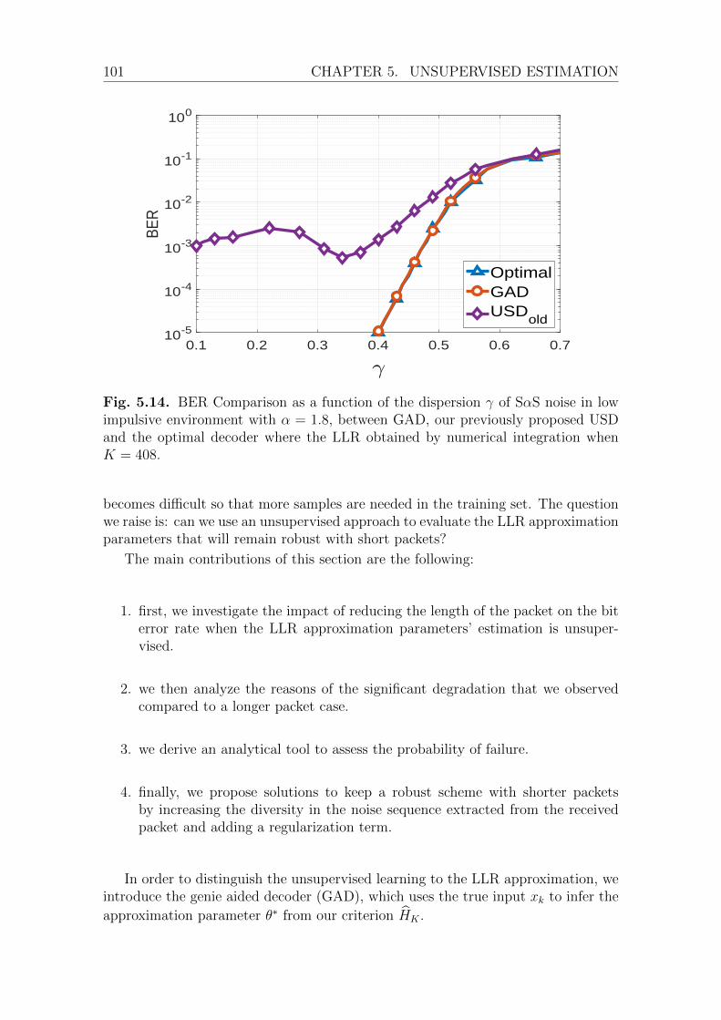
101 CHAPTER 5. UNSUPERVISED ESTIMATION
0.1 0.2 0.3 0.4 0.5 0.6 0.710-5
10-4
10-3
10-2
10-1
100
BER
OptimalGADUSD
old
Fig. 5.14. BER Comparison as a function of the dispersion γ of SαS noise in lowimpulsive environment with α = 1.8, between GAD, our previously proposed USDand the optimal decoder where the LLR obtained by numerical integration whenK = 408.
becomes difficult so that more samples are needed in the training set. The questionwe raise is: can we use an unsupervised approach to evaluate the LLR approximationparameters that will remain robust with short packets?
The main contributions of this section are the following:
1. first, we investigate the impact of reducing the length of the packet on the biterror rate when the LLR approximation parameters’ estimation is unsuper-vised.
2. we then analyze the reasons of the significant degradation that we observedcompared to a longer packet case.
3. we derive an analytical tool to assess the probability of failure.
4. finally, we propose solutions to keep a robust scheme with shorter packetsby increasing the diversity in the noise sequence extracted from the receivedpacket and adding a regularization term.
In order to distinguish the unsupervised learning to the LLR approximation, weintroduce the genie aided decoder (GAD), which uses the true input xk to infer the
approximation parameter θ∗ from our criterion HK .
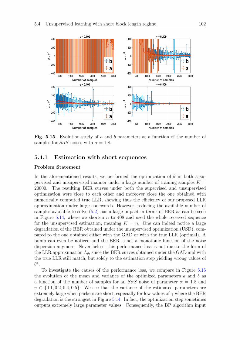
5.4. Unsupervised learning with short block length regime 102
Fig. 5.15. Evolution study of a and b parameters as a function of the number ofsamples for SαS noises with α = 1.8.
5.4.1 Estimation with short sequences
Problem Statement
In the aforementioned results, we performed the optimization of θ in both a su-pervised and unsupervised manner under a large number of training samples K =20000. The resulting BER curves under both the supervised and unsupervisedoptimization were close to each other and moreover close the one obtained withnumerically computed true LLR, showing thus the efficiency of our proposed LLRapproximation under large codewords. However, reducing the available number ofsamples available to solve (5.2) has a large impact in terms of BER as can be seenin Figure 5.14, where we shorten n to 408 and used the whole received sequencefor the unsupervised estimation, meaning K = n. One can indeed notice a largedegradation of the BER obtained under the unsupervised optimization (USD), com-pared to the one obtained either with the GAD or with the true LLR (optimal). Abump can even be noticed and the BER is not a monotonic function of the noisedispersion anymore. Nevertheless, this performance loss is not due to the form ofthe LLR approximation Lθ, since the BER curves obtained under the GAD and withthe true LLR still match, but solely to the estimation step yielding wrong values ofθ∗.
To investigate the causes of the performance loss, we compare in Figure 5.15the evolution of the mean and variance of the optimized parameters a and b asa function of the number of samples for an SαS noise of parameter α = 1.8 andγ ∈ 0.1, 0.2, 0.4, 0.5. We see that the variance of the estimated parameters areextremely large when packets are short, especially for low values of γ where the BERdegradation is the strongest in Figure 5.14. In fact, the optimization step sometimesoutputs extremely large parameter values. Consequently, the BP algorithm input

103 CHAPTER 5. UNSUPERVISED ESTIMATION
-(b/a)1/2 0 (b/a)1/2
y
-2
-1
0
1
2
L*(y
)
A-B- A+ B+
Fig. 5.16. Illustration of the LLR approximation with the four regions influencingthe shape of Lθ.
does not match the LLR, leading to poor BER. The same conclusion can be madefor other values of α.
In the rest of this section, we are going to (a) analyze in depth the reasons whythe estimation fails and (b) propose solutions to improve the robustness of this step.Thereafter we will call degeneration the fact that the optimization step outputs avery large value for parameters a or b, resulting in a bad tuning of Lθ∗ that does notmatch the real state.
Problem exploration
Let Z denote Z = XY . Z is an interesting way to present the following derivationbecause z > 0 means that x and y have the same sign (this bit detection would notbe in error) when z < 0 means that the noise modifies the sign of the transmittedbit. Since LLRs are odd functions, one can rewrite xΛ(y), respectively xLθ(y), asΛ(z) and Lθ(z). Further, let fab denote fab(z) = log2(1 + e−Lab(z)). Based on thetwo optimization parameters a and b and on the Lab approximation, one can definefour regions that influence the shape of Lθ as depicted in Figure 5.16:
B− =[−∞,−
√b/a]
;A− =[−√b/a, 0
];A+ =
[0,√b/a]
;B+ =[√
b/a,+∞].
(5.5)
Using these four regions, one can rewrite (3.19) as
H(X|Y )∝∑
zi∈B−∪B+
log2(1+e− bzi ) +
∑zi∈A−∪A+
log2(1+e−azi). (5.6)
In each of these regions, only one of the two optimization parameters influencesthe shape of Lθ: samples falling in B− and B+ are only impacting the optimizationparameter b, while samples falling in A− and A+ are only impacting the optimization

5.4. Unsupervised learning with short block length regime 104
parameter a. However, due to different exponent signs, minimizing H(X|Y ) requiresreverse optimization tendencies in the regions B+ and B−, respectively, A+ and A−.Indeed, samples zi in B− tend to decrease the value of b in order to minimize fab(zi)since b > 0 and zi < 0, whereas samples in B+ tend to increase the value of b, sincezi > 0. The optimal value of b results thus from a compromise between the two setsB+ and B−. The same analysis holds for the parameter a and one can conclude thatif one of these regions is empty, the minimization problem will converge towards anapproximated LLR far away from the true one.
Having empty A+ or empty B+ region is very unlikely since it would require allthe training samples to be decoded in error, or in other words to only have largenoise samples of the opposite sign than the input sequence. Hence only two casesremain that trigger the optimization failure:
1. empty B− region and populated B+ region: the samples in B+ will make bparameter goes to infinity in order to minimize fab. As a consequence, thethreshold
√|b/a| will increase and tend to infinity and thus the B− region
will still remain empty. This case, however, is not necessarily an optimizationfailure since under Gaussian noise, the optimal receiver is a linear one withb∗ → ∞. Under the GAD approach, such a case can also occur when nonegative z is received with a large amplitude.
2. empty A− region and populated A+ region: the terms in A+ will make aparameter goes to infinity in order to minimize fab. As a consequence, thethreshold
√|b/a| will decrease and tend to zero and thus the A− region will
remain empty. Under weak noise, the sign detector only extracts small noisesamples and thus the probability of having zero samples in A− becomes nonnegligible, leading thus to a very large value of a. The fact that it happensmore when the dispersion of the noise decreases explains the bump shapeobserved in Figure 5.14.
To conclude, the optimization step will fail when at least one of the aforemen-tioned regions is empty, which is more likely with short training sequences sincethe extracted noise does not represent its whole statistics. Indeed, impulsive noisesare characterized by large, but rare, events and their probability to appear severaltimes during the training sequence decreases when its length decreases. This can alsohappen in the unsupervised case, especially when the noise strength is low or/andwhen the impulsiveness is low. In fact, the sign detector will tend to generate noisesamples with values less than one.
Quantifying the risk of bad estimation
We will quantify the risk of optimization failure by assessing the probability of havingzero samples falling in the regions A− and B−. However, these two regions beingdelimited by a non-fixed boundary, we will relax the studied problem and considerthe case A− ∪B− = ∅, i.e. no negative samples z are obtained, which will be calleddegeneration.

105 CHAPTER 5. UNSUPERVISED ESTIMATION
The degeneration risk η is the probability that the sequence Z1, . . . , ZK has onlypositive elements:
ηk = P (Z > 0, ∀k ∈ 1, ..., K) . (5.7)
Let Qα denote the right tail of the probability function for a SαS random variableas Qα(x) =
∫ +∞x
fα(u)du, where fα is the probability density function of the SαSdistribution with dispersion parameter γ = 1.
Assuming K identically distributed and independent noise realizations, we have
η =K∏k=1
(1− P (Z ≤ 0)) = (1− P (Z ≤ 0))K . (5.8)
In the next Proposition, we will provide the degeneration risk under both theGAD and the unsupervised approach.
Proposition 5. Under the Genie-aided decoder, the degeneration risk is given as
ηK,GAD =
[1−Qα
(1
γ
)]K= (η1,GAD)K , (5.9)
whereas under the unsupervised optimization, it is given as
ηK,USD =
[1− 1
2Qα
(3
γ
)− 1
2Qα
(1
γ
)]K=(η1,USD)K . (5.10)
Proof. Let us consider the two cases separately.Under the GAD, X ∈ −1, 1 and Y = X + N , so that Z = XY is negative if
X = +1 and N < −1 or if X = −1 and N > 1. Thus,
P (Z < 0) =1
2P (N < −1|x = +1) +
1
2P (N > 1|x = −1)
=1
2
(∫ −1
−∞fα(u)du+
∫ +∞
1
fα(u)du
)= Qα
(1
γ
), (5.11)
and ηK,GAD =
[1−Qα
(1γ
)]K= (η1,GAD)K .
It should be emphasized that, due to the full access to a genie-aided providedbits X, the estimation failure will be triggered only when no negative sample existswhich translates in this case as an error-free received codeword. Thus, the BERperformance will not be influenced in spite of a badly tuned LLR approximation.
Under unsupervised optimization, the training sequence only consists of X = +1sand Y = +1 + N . As a consequence, the probability to have a negative Z = XY is
P(Z < 0
)= P
(N < −1
)= P (Y − sign (Y ) < −1) .

5.4. Unsupervised learning with short block length regime 106
.
0.1 0.2 0.3 0.4 0.5 0.6 0.7 0.8
2
0.82
0.84
0.86
0.88
0.9
0.92
0.94
0.96
0.98
USD, ,=1.8GAD, ,=1.8USD, ,=1.4GAD, ,=1.4
1
Fig. 5.17. Degeneration risk for K = 1 and α = 1.4 or 1.8 for the USD andthe GAD receivers. It is important to notice the gap between the two approaches,explaining the gap between the BER obtained with USD and the one obtained withGAD.
Necessarily, sign (Y ) = −1 since sign (Y ) = 1 would lead to Y < 0 which is incontradiction. Thus,
P(Z < 0
)= P (X +N < −2)
=1
2P (N < −3|X = 1) +
1
2P (N < −1|X = −1)
=1
2
[Qα
(3
γ
)+Qα
(1
γ
)]. (5.12)
Finally, we have ηK,USD=
[1− 1
2Qα
(3γ
)− 1
2Qα
(1γ
)]K=(η1,USD)K .
Discussion
In Figure 5.17, we represent the degeneration risk for K = 1 for the genie-aideddecoder as well as for the unsupervised decoder (USD) as given in Proposition 5.Note that the degeneration risk is only a qualitative measure which gives an idea ofthe probability of badly estimating a and b: when the value of this risk decreases, itindicates that region A− ∪B− has a higher probability to contain samples and thusthe estimation to converge.
Based on this numerical simulation, three conclusions can be made:
1. The degeneration risk under USD is significantly higher than under GAD,which shows that the estimation will be more difficult in the unsupervisedsetting and explains the BER degradation observed in Figure 5.14.

107 CHAPTER 5. UNSUPERVISED ESTIMATION
2. The degeneration risk increases when γ decreases. The dispersion γ is a scaleparameter that measures the spread of the samples around the mean, similarlyto the variance in the Gaussian case. Figure 5.17 shows that an estimationfailure (ηK tends to 1) is inevitable when the noise dispersion is small, making
all samples falling close to the mean (in our case X = 1). Thus, it is lesslikely to have samples in A− ∪B−. The consequence is most significant in themedium and low γ regions. That consequence explains the bump observed inFigure 5.14.
3. The degeneration risk decreases as α becomes smaller (more impulsive). In-deed, the smaller the value of α, the heavier the tail of the probability densityfunction, which increases the likelihood of having impulses with large ampli-tudes and far from the central location. Thus, it is more likely to have samplesin A− ∪B−.
These aspects are not intuitive because they suggest that the reduction of thepacket length will be more detrimental when noise is less impulsive and with asmaller strength. However, If the noise strength is low, its impact will be very lowand even if the estimation is not accurate, the decoding should succeed. Neverthe-less, the most impacting regime is the medium noise strength regime, in which thebump can be observed on the BER curves.
In the following, we propose a new training sequence Y design to reduce thedegeneration risk under the unsupervised optimization.
5.4.2 Proposed solution for the estimation with short blocklength
We now provide two mechanisms in order to decrease the degeneration risk obtainedunder unsupervised optimization: one regularization term in order to prevent theparameter a to tend to infinity and one algorithm to increase the diversity in theextracted noise sequence, such that the convergence of the parameter b is improved.
I Parameter a: the value of a defines the slope of the linear part for low valuesof the received signal y. Thus, if this parameter tends toward infinity, theapproximated LLR would tend towards b/y which gives the highest likelihoodin samples around 0, which obviously is not efficient. To overcome this issue,we propose to add a regularization term to (5.6) such that reasonable valuesfor a are obtained even if A− is empty. The new objective function writes as
H(X|Y )New = H(X|Y ) + log2(1 + eaε), (5.13)
where ε is a small value. The regularization term corresponds to an artifi-cial small negative sample of amplitude ε in the A− region. It prevents anempty A− region that causes degeneration. With small ε, this term could beapproximated by a linear regularization log2(1 + eaε) ≈ aε/(2 log 2).
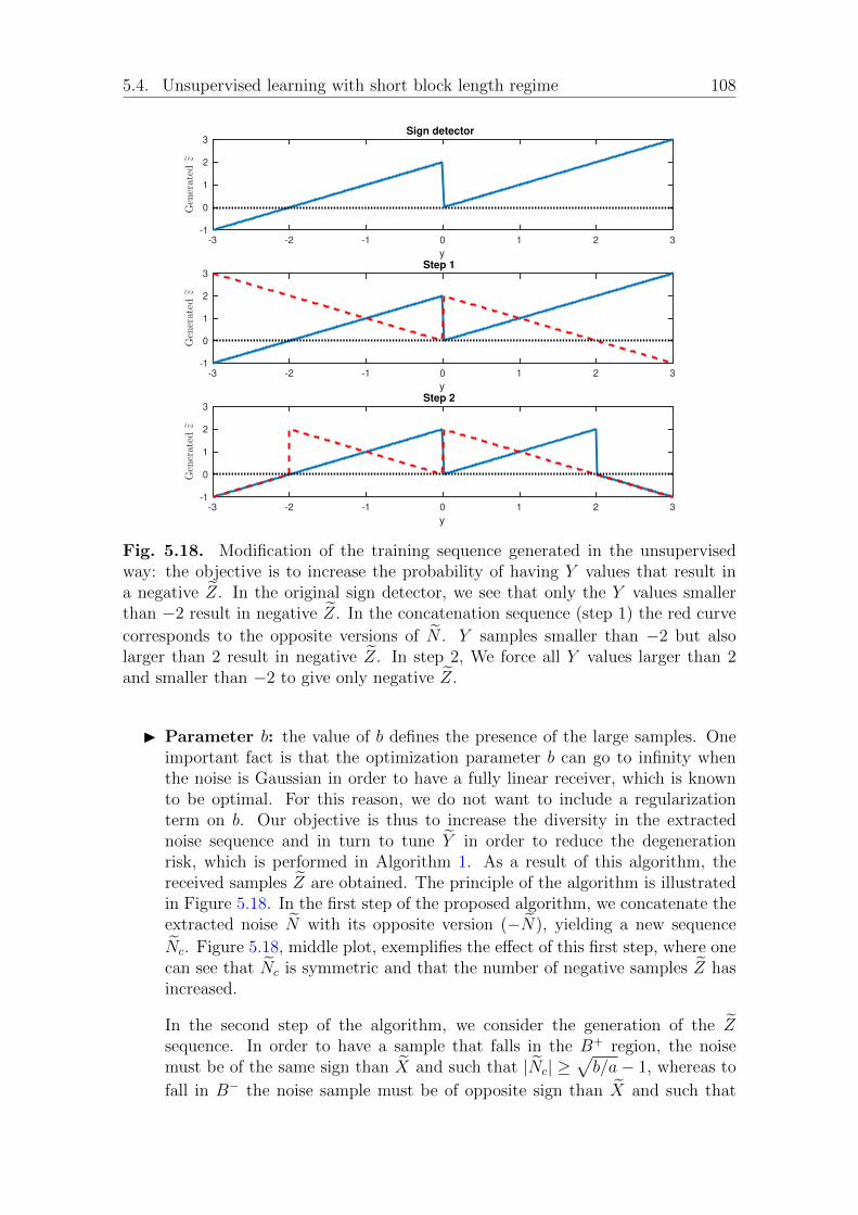
5.4. Unsupervised learning with short block length regime 108
-3 -2 -1 0 1 2 3
y
-1
0
1
2
3
Generatedz
Sign detector
-3 -2 -1 0 1 2 3
y
-1
0
1
2
3
Generatedz
Step 1
-3 -2 -1 0 1 2 3
y
-1
0
1
2
3
Generatedz
Step 2
Fig. 5.18. Modification of the training sequence generated in the unsupervisedway: the objective is to increase the probability of having Y values that result ina negative Z. In the original sign detector, we see that only the Y values smallerthan −2 result in negative Z. In the concatenation sequence (step 1) the red curve
corresponds to the opposite versions of N . Y samples smaller than −2 but alsolarger than 2 result in negative Z. In step 2, We force all Y values larger than 2and smaller than −2 to give only negative Z.
I Parameter b: the value of b defines the presence of the large samples. Oneimportant fact is that the optimization parameter b can go to infinity whenthe noise is Gaussian in order to have a fully linear receiver, which is knownto be optimal. For this reason, we do not want to include a regularizationterm on b. Our objective is thus to increase the diversity in the extractednoise sequence and in turn to tune Y in order to reduce the degenerationrisk, which is performed in Algorithm 1. As a result of this algorithm, thereceived samples Z are obtained. The principle of the algorithm is illustratedin Figure 5.18. In the first step of the proposed algorithm, we concatenate theextracted noise N with its opposite version (−N), yielding a new sequence
Nc. Figure 5.18, middle plot, exemplifies the effect of this first step, where onecan see that Nc is symmetric and that the number of negative samples Z hasincreased.
In the second step of the algorithm, we consider the generation of the Zsequence. In order to have a sample that falls in the B+ region, the noisemust be of the same sign than X and such that |Nc| ≥
√b/a− 1, whereas to
fall in B− the noise sample must be of opposite sign than X and such that

109 CHAPTER 5. UNSUPERVISED ESTIMATION
Data: Channel output YResult: Z/* Step-1 */
N = Y − sign(Y )
Nc = −N ||N % Concatenate N and −N into Nc; /* Step-2 */
for k=1 to length(Nc) do
if Nc(k) ≥ 1 then
Z(k) = +1− Nc(k)else
Z(k) = +1 + Nc(k)end
end
Algorithm 1: Generating the training sequence Z = +1.Y
|Nc| ≥√b/a+1. The probability of this second event is much smaller than the
probability of the first: having samples in B+ is highly probable but havingan empty B− has also a high probability. To reduce this last probability, weforce a negative Z when |Nc| > 1.
The next proposition states the degeneration risk of our new training design, allowingthus to evaluate its benefits.
Proposition 6. Under the new training sequence design with unsupervised opti-
mization, the degeneration risk is given as ηK,NUSD =
[1−Qα
(3γ
)−Qα
(1γ
)]K=
(η1,NUSD)K .
Proof. under this new design, Z is given either as Z = 1 ± Nc, depending on thevalue of Nc, thus
P (Z < 0) = P (Z < 0, N ≥ 1) + P (Z < 0, N ≤ −1)
+ P (Z < 0,−1 ≤ N ≤ 1)
= P (Z < 0, N ≥ 1) + P (Z < 0, N ≤ −1)
= P (N ≥ 1) + P (N ≤ −1)
= 2(P (N < −1)
)= Qα
(3
γ
)+Qα
(1
γ
)(5.14)
and ηK,NUSD =
[1−Qα
(3γ
)−Qα
(1γ
)]K= (η1,NUSD)K .
Discussion
Figure 5.19 compares the degeneration risk ηK of the GAD and USD as a functionof γ under an additive impulsive SαS noise with α ∈ 1.8; 1.4 representing low

5.4. Unsupervised learning with short block length regime 110
.
0.1 0.2 0.3 0.4 0.5 0.6
2K
10-5
100,=1.8.
0.1 0.2 0.3 0.4 0.5 0.6
2K
10-5
100,=1.4
USD-OldGADUSD-New
Fig. 5.19. Comparison of the degeneration risk ηK for GAD, the simple signdetector USD or the new unsupervised case NUSD as a function of γ, under SαSnoise with α = 1.8 and α = 1.4 representing less and high impulsive environments,respectively and with K = 408.
and high impulsive environments respectively. The block size considered is 408which depicts short codewords. The new unsupervised approach, which improvesthe diversity in the generated Z sequence, allows to significantly decrease ηK , whichgets even smaller than the one under the GAD. Nevertheless, this does not guaranteebetter BER performance but only that the estimation should be more robust fromone packet to another.
In Figure 5.20, we provide the evolution of the mean and the variance of theoptimization parameters a and b under our proposed approach, which can be com-pared to the one obtained in Figure 5.15 without the two mechanisms allowing thedegeneration risk decrease. One can note that under our proposed method, the op-timization parameters do converge for all values of the noise strength. Even if theparameter b still exhibits some variability, it is significantly reduced: the variationsaround the mean values are much more confined compared to the previous methodand will not result in catastrophic values. The threshold
√|b/a| remains stable so
that the shape of the LLR remains similar whatever the training set. It shouldbe mentioned that similar conclusions are observed for other values of α or otherimpulsive environment types, as for instance, Middleton Class A, ε-contaminated orGaussian noise.
In the following, we present some numerical simulations showing the performanceof our new designed training sequence under blind optimization.

111 CHAPTER 5. UNSUPERVISED ESTIMATION
500 1000 1500 2000 2500 3000
Number of samples
0
10
20
30
, 2
= 0.100
ba
500 1000 1500 2000 2500 3000
Number of samples
0
10
20
30
, 2
= 0.200
ba
500 1000 1500 2000 2500 3000
Number of samples
5
10
15
, 2
= 0.400
ba
500 1000 1500 2000 2500 3000
Number of samples
4
6
8
10
, 2
= 0.500
ba
Fig. 5.20. Evolution study of a and b parameters using the proposed solution as afunction of the number of samples for SαS noise with α = 1.8.
5.4.3 Numerical results using LDPC codes
Simulation Setup
We assume that the input sequence is encoded using a regular (3,6) LDPC code ofsize n = 408. Consequently, the available number of samples to solve (3.14) is setto K = 408, allowing to assess the performance gain of the new training sequencedesign in the short codeword regime. In order to assess the robustness of our method,we will consider the five following noisy environments:
I low impulsive SαS environment with α = 1.8 in Figure 5.21;
I high impulsive SαS environment with α = 1.4 in Figure 5.22;
I Gaussian noise in Figure 5.23;
I moderate impulsive Middleton environment with A = 0.1 and Γ = 0.1 inFigure 5.25.
I high impulsive Middleton environment with A = 0.01 and Γ = 0.01 in Fig-ure 5.24.
I low impulsive ε−contaminated environment with ε = 0.01 and K = 10 inFigure 5.26.
I high impulsive ε−contaminated environment with ε = 0.1 and K = 10 inFigure 5.27.
Under all noise types, we provide the BER curves obtained with the GAD,with the unsupervised optimization with our previously proposed training sequence

5.4. Unsupervised learning with short block length regime 112
0.1 0.2 0.3 0.4 0.5 0.6 0.710-5
10-4
10-3
10-2
10-1
100B
ER
OptimalGADUSD
new
USDold
Fig. 5.21. BER evolution as a function of γ under a low impulsive SαS noise withα = 1.8
0.1 0.2 0.3 0.4 0.5 0.6 0.7
10-6
10-4
10-2
100
BE
R
OptimalGADUSD
new
USDold
Fig. 5.22. BER evolution as a function of γ under a high impulsive SαS noise withα = 1.4

113 CHAPTER 5. UNSUPERVISED ESTIMATION
Fig. 5.23. BER evolution as a function of Eb/N0 under a Gaussian noise
design [MSG+18,MSG+19d] (USD old) as well as with the newly proposed trainingsequence (USD new). We furthermore provide the BER curves obtained with thenumerically obtained true LLR to represent the best possible case with the givencode and BP. Under SαS noises, we present the BER curves as a function of thedispersion γ; whereas under the Gaussian, Middleton and ε-contaminated cases, wepresent the BER curves a function of the signal-to-noise ration Eb/N0.
Discussion
Under all types of noises, impulsive or not, the GAD reaches the optimum, provingthe validity of the LLR approximation choice Lθ under the short packet assumption.It seems unnecessary in that case to use a more accurate approximation, as Labc thatwas proposed in Section 4.2.3. Moreover, under the old training sequence design, theBER curve is not monotonic and exhibits a bump due to the degeneration explainedin Section 5.4.1, whereas the BER curve obtained under the new training sequencedesign is close to the one obtained with GAD. The new training sequence improvesthe performance of the optimization step under short codewords for all types of ad-ditive noise, impulsive or not, without requiring the noise model knowledge at thereceiver. Furthermore, our method does not decrease the performance under Gaus-sian noise, where the optimal b parameter should be infinite. Thus, our proposedmethod allows to achieve almost optimal BER performance for noises ranging fromhighly impulsive, moderately impulsive to Gaussian, with a low implementationcomplexity without the knowledge of the noise model, even with a small availablenumber of data samples to perform the LLR approximation optimization.

5.4. Unsupervised learning with short block length regime 114
Fig. 5.24. BER evolution as a function of Eb/N0 under a high impulsive Middletonnoise with A = 0.01 and Γ = 0.01.
Fig. 5.25. BER evolution as a function of Eb/N0 under a moderate impulsiveMiddleton noise with A = 0.1 and Γ = 0.1.
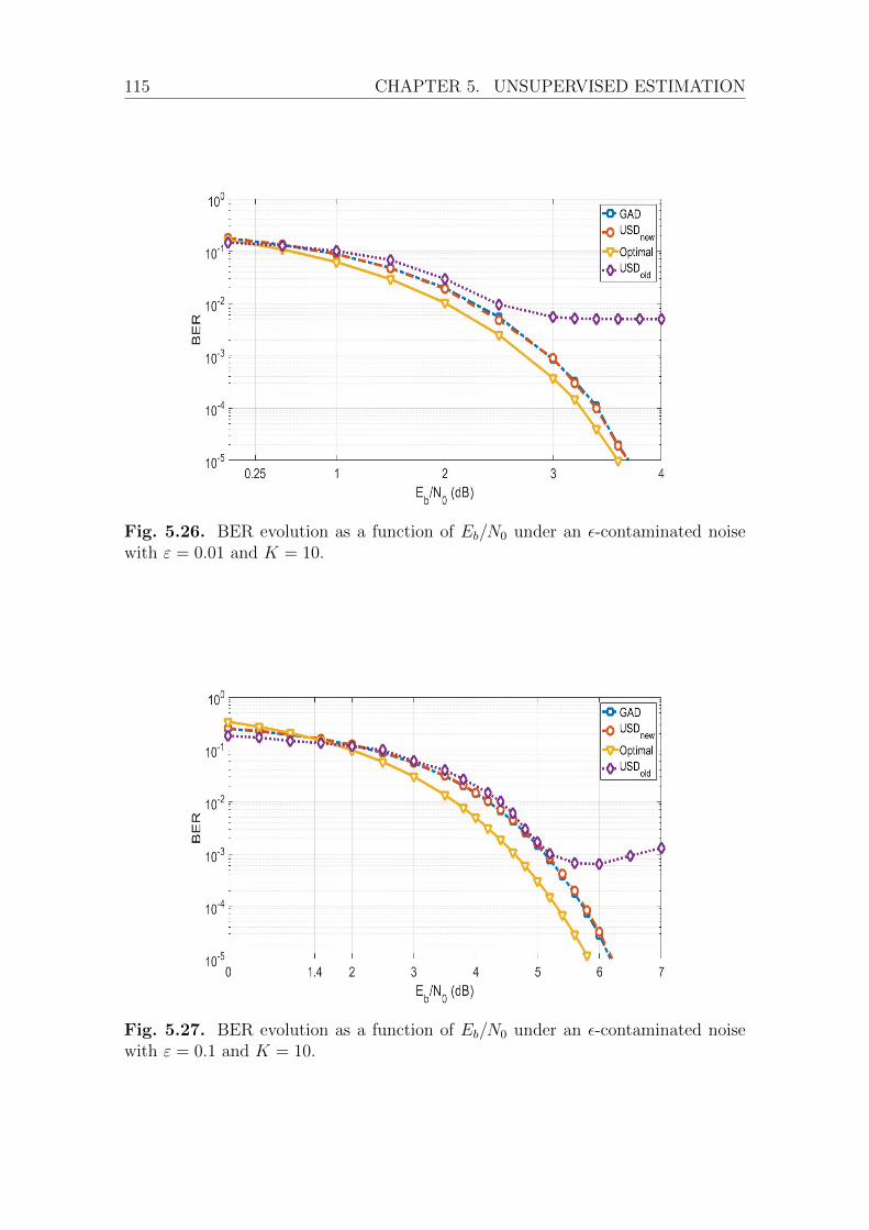
115 CHAPTER 5. UNSUPERVISED ESTIMATION
Fig. 5.26. BER evolution as a function of Eb/N0 under an ε-contaminated noisewith ε = 0.01 and K = 10.
Fig. 5.27. BER evolution as a function of Eb/N0 under an ε-contaminated noisewith ε = 0.1 and K = 10.
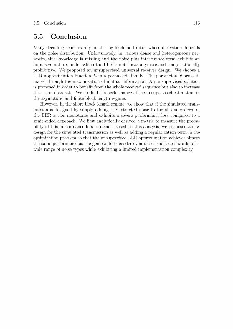
5.5. Conclusion 116
5.5 Conclusion
Many decoding schemes rely on the log-likelihood ratio, whose derivation dependson the noise distribution. Unfortunately, in various dense and heterogeneous net-works, this knowledge is missing and the noise plus interference term exhibits animpulsive nature, under which the LLR is not linear anymore and computationallyprohibitive. We proposed an unsupervised universal receiver design. We choose aLLR approximation function fθ in a parametric family. The parameters θ are esti-mated through the maximization of mutual information. An unsupervised solutionis proposed in order to benefit from the whole received sequence but also to increasethe useful data rate. We studied the performance of the unsupervised estimation inthe asymptotic and finite block length regime.
However, in the short block length regime, we show that if the simulated trans-mission is designed by simply adding the extracted noise to the all one-codeword,the BER is non-monotonic and exhibits a severe performance loss compared to agenie-aided approach. We first analytically derived a metric to measure the proba-bility of this performance loss to occur. Based on this analysis, we proposed a newdesign for the simulated transmission as well as adding a regularization term in theoptimization problem so that the unsupervised LLR approximation achieves almostthe same performance as the genie-aided decoder even under short codewords for awide range of noise types while exhibiting a limited implementation complexity.

Chapter 6Conclusion and perspectives
This thesis focused on designing a robust receiver that exhibits a near-optimalperformance over Gaussian and non-Gaussian environments without relying on
the knowledge of interference plus noise statistical properties. This receiver strivesfor universality by adapting automatically to a large variety of different conditions.Such receivers can play an important role in future networks that will face twocrucial challenges, robustness and adaptability, in a highly interfering environmentand with strict energy and lifetime constraints.
We have shown in our work that a simple module between the channel outputand the decoder input allows to combat effectively the noise and interference thatdisrupt point-to-point communications in a network. This module can be used asa front end of any LLR-based decoder. It consists of a function approximating thecalculation of the likelihood ratio, which is rarely accessible and that requires theknowledge of the channel status. However, thanks to a judicious criterion, it ispossible to search for this approximation function effectively either by supervisedlearning or by an unsupervised one. We show that it is even possible to use such ascheme for short packet communications without performance losses.
The perspectives of our work are many. To start with we can give some issuesthat have not been really discussed in the thesis but would deserve some attention.For instance, the complexity issues are not properly addressed and if we think thatour demapper would not significantly increase the decoding complexity, it should becarefully analyzed. In the short term, it is relevant to extend our results for higherorder modulations such as quadrature amplitude modulations (QAM). In this case,the likelihood ratios depend on the position of the bits in the binary coding of thesymbols. It is, therefore, necessary to propose families of functions that take intoaccount this position. Our preliminary works show that it is possible to return to amixture of our functions Lab to limit the size of the parameters or even to use theLabc. Figure 6.1 shows an example of a gray coded 16-QAM constellation as shownin plot (a) and the corresponding LLR for the first and second most significant bitsshown in plot (b), where the received samples Y is influenced by a SαS noise. Forinstance, the LLR of the first bit Lb1 can be approximated as
Lb1 = max Lab(y), Lab(y − 2) ,

118
0 01
0 1
00 00 10 00
00 01
00 11
00 10
10 01
01 00
01 01
01 11
01 00
11 00
11 01
11 11
11 10
10 11
10 10
Bit # 1
Bit # 2
I
LLR Bit #1
LLR Bit #2
𝛂 = 𝟏. 𝟒 ; 𝛄 = 𝟎. 𝟑
𝐘
𝐋𝐋𝐑(𝐘)
(a) Gray coded 16-QAM constellation. (b) LLR computation for the first and second most significant bits.
12 34xx xx
Fig. 6.1. Example of a LLR-computation for higher-order constellations (16-QAM)
or perhaps simply by using Labc.Another promising perspective is to integrate the LLR approximation to the code
design. The LLR may uniformize the distribution of the messages coming from thechannel outputs for several impulsive noises. Looking for a good code candidatewill reduce the gap between the performances and channel capacity, which, as wehave shown, is sometimes rather large. Of course, the asymptotic limit should bereplaced by the short block length regime bound proposed by Polyanskiy [PPV10]to have a better insight on the gain that can be reached (section 5.4.3), this is anon-going work.
In the longer term, since the proposed criterion is close to a variational approachto learning, it may be appropriate to integrate it directly into channel decoding sothat there is an exchange of information between the code and the LLR calculation.This is all the more relevant as in the unsupervised case, limiting the number ofdecision errors improves the quality of the noise samples obtained and therefore theestimation of the parameters. A simple joint coupling between channel decoding andLLR approximation has already been tested but we did not observe any significantimprovement. However, it deserves more detailed analysis, for example by usinga coupling of factor graphs between that of the LDPC code and that of the LLRapproximation.
Besides, we have always considered approximations that belong to a certain fam-ily built a priori. Since the criterion comes from information theory, it would bebeneficial to make the approach even more generic by choosing a function accord-ing to Jaynes [Jay03] maximum entropy approach and combining it with channeldecoding directly to make a decoder based on the principle of maximum entropy.
Also, it has been shown that interference can exhibit a non-trivial dependencestructure, especially some tail dependence [ZEC+19]. How to account for this depen-dence is an interesting open question that could significantly impact the robustness

119 CHAPTER 6. CONCLUSION AND PERSPECTIVES
of the communication.

120
121 ANNEXE A. RESUME DETAILLE EN FRANCAIS
Annexe AResume detaille en francais
A.1 Introduction
A.1.1 Contexte
Lors de communications filaires, l’agitation thermique au niveau du recepteur ex-plique en grande partie les bruits perturbant les signaux porteurs d’information.Le theoreme central limite sert alors de justification a leur modelisation par undis-tribution gaussienne centree. En effet, l’agitation thermique consiste en un grandnombre de fluctuations centrees independantes et de puissance finie qui correspondaux premisses du theoreme.
Les communications sans fils et en reseau subissent en plus du bruit thermiquedes interferences avec les communications voisines qui ne peuvent pas etre considereescomme du bruit independant et gaussien. Plusieurs techniques ont ete developpeespour les limiter comme l’alignement d’interferences au niveau de la couche phy-sique [EPH13] ou des techniques d’evitement de transmissions simultanees commele CSMA au niveau de la couche MAC [YV05,JHMB05]. Enfin, d’autres methodesessaient de les supprimer efficacement au niveau du recepteur comme l’annulationsuccessives d’interferences (SIC) [WAYd07,And05].
Toutes ces techniques ne peuvent parfaitement annuler les et divers. Cela severifie d’autant plus que nous nous dirigeons vers des reseaux denses comme LoRa,Sigfox, la 5G ou en general l’IoT sans controle centralise ni d’acces a la ressourceradio ni aux puissances des emissions.
Par consequent, prendre en compte la presence des interferences au niveau durecepteur devient une necessite, voire une obligation. Une modelisation fine et pra-tique des interferences s’avere alors un prerequis pour concevoir la chaıne de reception.Plusieurs approches ont ete envisagees dans la litterature pour construire ces modeles.La premiere, tournee vers la theorie, consiste a utiliser les outils mathematiquescomme la geometrie aleatoire [WA12,WPS09] avec des hypotheses sur la conceptionet l’utilisation du reseau pour en deduire des modeles pertinents. Ces travaux menentpar exemple aux modeles alpha-stables [PW10a,GCA+10] ou aux differentes classesdes modeles de Middleton [Mid77]. Le second type d’approche est plus pragmatique :il s’agit de trouver des familles de lois de probabilite qui soient simples d’utilisationet qui correspondent aux aspects impulsifs des interferences. Ces lois doivent avoir

A.2. Description du systeme 122
une queue lourde pour modeliser les evenements impulsifs qui se caracterisent pardes valeurs de forte amplitude. Parmi ces modeles nous retrouvons les gaussiennesgeneralisees ou les melanges de gaussiennes.
Nous avons concentre particulierement nos travaux sur les distributions alpha-stables symetriques et centrees comme modele des interferences meme si d’autresmodeles ont ete utilises pour tester nos solutions.
A.1.2 Objectifs et contributions
L’objectif principal de nos travaux consiste a developper un recepteur simple, adap-tatif et performant qui prenne en compte le caractere impulsif des interferences vuescomme un bruit additif. Simplicite signifie ici une mise en œuvre peu couteuse entemps de calcul et en memoire. Le caractere adaptatif necessite de prendre en comptel’etat reel du canal sans le connaıtre par ailleurs ; pour cela un apprentissage devientnecessaire. Enfin, les performances ne doivent pas s’ecarter de l’optimum fourni parle log rapport de vraisemblance.
Nous avons repondu a ces objectifs par nos contributions qui sont
I l’ajout d’une approximation directe du rapport de vraisemblance entre la sortiedu canal et le decodeur de canal ;
I la proposition d’un critere pertinent pour l’adaptation de cette approximationselon le type de bruit et d’interference ;
I l’utilisation de ce critere pour le developpement d’un algorithme d’adaptationsupervise, c’est-a-dire base sur une sequence d’apprentissage ;
I l’analyse de cet algorithme sur les criteres de performances et de robustesseselon la longueur de la sequence d’apprentissage ;
I l’extension de cet algorithme a un apprentissage non supervise et son etude ;
I l’amelioration de l’apprentissage non supervise dans le cadre des communica-tions a paquets courts.
A cela s’ajoute la proposition d’une nouvelle famille de fonctions d’approximationa trois parametres plus performantes mais restant toujours simples et la propositiond’un critere plus simple reliant la divergence de Kullback-Leibler avec la norme L2
pour comparer les recepteurs.
A.2 Description du systeme
Nos travaux reposent sur un bruit modelise par les distributions alpha-stables etsur un systeme qui utilise les codes LDPC. Ces deux points sont discutes dans cettesection pour finir par la specification du modele de canal considere.

123 ANNEXE A. RESUME DETAILLE EN FRANCAIS
Fig. A.1. Exemple de realisations de bruit alpha-stable.
A.2.1 Distributions alpha-stables
Les distributions alpha-stables sont les distributions limites des sommes de variablesaleatoires normalisees et centrees lorsqu’elles existent [GH97]. Nous nous limiteronspar la suite aux versions symetriques, et, dans cette situation, ces distributionslimites se decrivent par leur fonction caracteristique
φ(t) = e−|γ t|α
, (A.1)
parametree par leur exposant caracteristique α et leur facteur d’echelle γ. Parmi cesdistributions se trouvent les lois normales avec α = 2 et γ = σ/
√2 et les distributions
de Cauchy avec α = 1 et γ = 1/a.
Quelques realisations de bruits selon les distributions alpha-stables sont representeessur la figure A.1. Il est visible que le parametre α caracterise l’impulsivite du bruit :plus α est faible plus la probabilite d’avoir des echantillons de forte amplitude aug-mente ainsi que la valeur de ces amplitudes.
Des densites de probabilite de lois alpha-stables pour differentes valeurs de αsont tracees sur la figure A.2. Elle illustre bien le caractere “queues lourdes” de cesmodeles qui permet de prendre en compte le caractere impulsif des interferences. Lecas gaussien α = 2 se particularise vraiment car la probabilite des grandes ampli-tudes decroıt exponentiellement et non plus selon une loi inverse comme pour lesautres α.
Bien qu’attrayantes les distributions stables souffrent de deux defauts impor-tants. Le premier concerne leur variance qui est infinie lorsque α < 2. Par consequent,la notion de rapport sur bruit devient inoperante et c’est pourquoi, pour indiquerl’intensite des interferences nous utiliserons plutot le facteur d’echelle γ. Le seconddefaut est l’absence d’expression simple de la densite de probabilite en general ; pour

A.2. Description du systeme 124
Fig. A.2. Densite de probabilite de lois alpha-stables.
la calculer il faut avoir recours a des integrations numeriques approchees calculantla transformee de Fourier inverse de la fonction caracteristique (A.1).
A.2.2 Codes LDPC
Nos travaux permettent de transformer la sortie du canal perturbee par des in-terferents et du bruit pour qu’elle soit utilisable pour la suite de la reception. Pourpouvoir mesurer les performances obtenues, il est necessaire de recourir a un codecorrecteur d’erreurs. Le choix s’est naturellement porte vers les codes LDPC pourplusieurs raisons : ils forment une famille simple a decrire et performante pour unelarge gamme de longueurs de mots de code. L’algorithme de propagation de croyanceappele Sum Product Algorithm permet une mise en œuvre generique qui utilise di-rectement en entree les log rapports de vraisemblance (LLR) de la sortie du canal.Ainsi, nos travaux s’implementent comme un element de la chaıne entre la sortie ducanal sous la forme du signal et du bruit et le decodeur LDPC sous la forme d’unLLR.
Les performances d’une chaıne avec un code LDPC suivent generalement le tracede la figure A.3. La region de decroissance rapide du taux d’erreur s’appelle la regiondu waterfall qui est suivie par une stagnation de cette decroissance, la region duplancher d’erreur (error floor).
La suite du manuscrit ne concerne pas specifiquement les codes LDPC et nousne nous etendrons pas sur ce point. Toutefois, nous utiliserons dans nos simulationsles codes regulier (3, 6) de MacKay de longueur 20000 et de longueur 408 construitpar l’algorithme du PEG [XEA05].
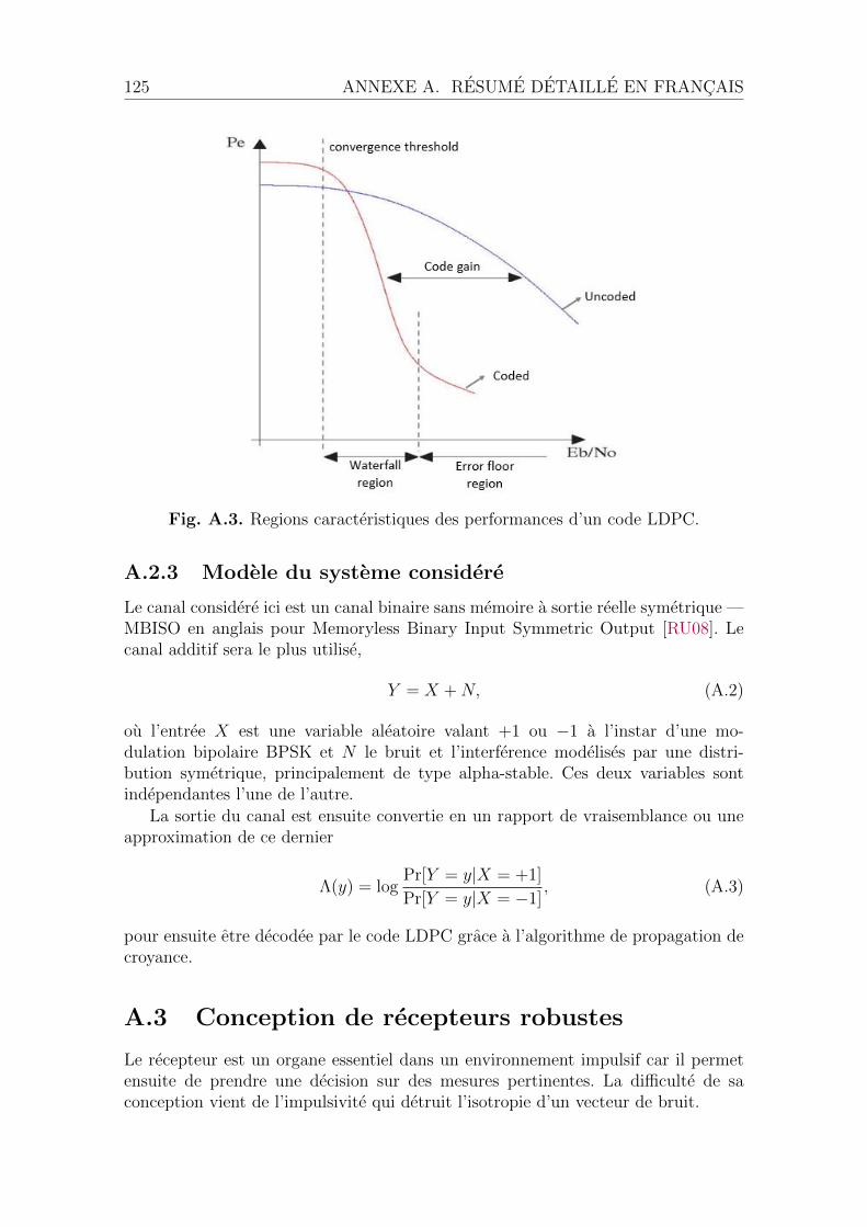
125 ANNEXE A. RESUME DETAILLE EN FRANCAIS
Fig. A.3. Regions caracteristiques des performances d’un code LDPC.
A.2.3 Modele du systeme considere
Le canal considere ici est un canal binaire sans memoire a sortie reelle symetrique —MBISO en anglais pour Memoryless Binary Input Symmetric Output [RU08]. Lecanal additif sera le plus utilise,
Y = X +N, (A.2)
ou l’entree X est une variable aleatoire valant +1 ou −1 a l’instar d’une mo-dulation bipolaire BPSK et N le bruit et l’interference modelises par une distri-bution symetrique, principalement de type alpha-stable. Ces deux variables sontindependantes l’une de l’autre.
La sortie du canal est ensuite convertie en un rapport de vraisemblance ou uneapproximation de ce dernier
Λ(y) = logPr[Y = y|X = +1]
Pr[Y = y|X = −1], (A.3)
pour ensuite etre decodee par le code LDPC grace a l’algorithme de propagation decroyance.
A.3 Conception de recepteurs robustes
Le recepteur est un organe essentiel dans un environnement impulsif car il permetensuite de prendre une decision sur des mesures pertinentes. La difficulte de saconception vient de l’impulsivite qui detruit l’isotropie d’un vecteur de bruit.

A.3. Conception de recepteurs robustes 126
Fig. A.4. Regions de decision optimale pour differents type de bruit.
A.3.1 Regions de decision et impulsivite
Considerons la reception d’un signal valant +1 ou −1 et dont on recupere la valeurdeux fois y1 et y2 mais bruitee par deux realisations independantes de bruit impulsif.
La figure A.4 montre les regions de decision en fonction des valeurs mesurees y1 ety2 pour differents types de bruit. La region blanche indique une decision pour l’envoide +1 et la region noire pour −1. Lorsque le bruit est gaussien, vignette en hauta gauche, les regions sont particulierement simples car separees par la mediatricedes points (+1,+1) et (−1,−1). Par contre, en presence d’impulsivite, les regionsde decision ne sont plus necessairement connexe comme en temoignent les autresvignettes ou le bruit est soit un melange de gaussiennes, soit la somme d’un bruitalpha-stable et d’un bruit gaussien. Dans ces cas, contrairement au cas gaussien, ladistance aux points (+1,+1) et (−1,−1) n’est plus suffisante pour decider, il fautajouter une information sur la direction des valeurs recues. En ce sens, la brisured’isotropie du vecteur bruit deconnecte les regions de decision.
A.3.2 Conception de recepteur
Pour repondre aux difficultes de detection en environnement impulsif, il est necessairede revenir au rapport de vraisemblance qui est une statistique suffisante [CT06]. Au-trement dit, l’objectif du recepteur, encore appele parfois demappeur, est de calculerle LLR Λ(y) donne par (A.3).
Dans le cas d’un canal MBISO, ce LLR represente a la fois le rapport de vraisem-blance mais aussi le rapport des probabilites a posteriori car l’a priori est uniforme,
Λ(y) = logPr[Y = y|X = +1]
Pr[Y = y|X = −1]= log
Pr[X = +1|Y = y]
Pr[X = −1|Y = y], (A.4)
et comme X est binaire et uniforme, la donnee du LLR est equivalente a celle de l’a

127 ANNEXE A. RESUME DETAILLE EN FRANCAIS
posteriori
Pr[X = x|Y = y] =1
1 + e−x Λ(y). (A.5)
Malheureusement, pour evaluer Λ(y), il est necessaire de connaıtre la distributiondu bruit affectant le canal. En effet, pour un bruit additif, le LLR s’ecrit Λ(y) =log[p(y− 1)/p(y+ 1)
]ou p(·) est la densite de probabilite du bruit. Or cette densite
est inconnue du recepteur.Plusieurs strategies sont envisageables pour calculer le LLR. La premiere consiste
a presupposer un modele de bruit, par exemple gaussien ou alpha-stable, parametrepar des coefficients qui seront estimes a partir de la sortie du canal. Par exemple,dans le cas gaussien, il est necessaire d’estimer la puissance du bruit et dans lecas alpha-stable l’exposant caracteristique et le facteur d’echelle doivent etre ob-tenus par ailleurs. Cette strategie est limitee d’une part par la difficulte d’obtenirdes estimations des parametres suffisamment fiables notamment dans un environ-nement impulsif et d’autre part par une mauvaise modelisation du bruit du canal.Par exemple, utiliser un modele gaussien dans un environnement impulsif s’averedesastreux en terme de performances [MGCG10a, MGCG13]. Enfin, lorsque l’ex-pression de la densite de probabilite du bruit n’est pas une expression simple, lecalcul du LLR s’avere soit couteuse en temps soit en espace pour mettre en placedes un systeme pre-calcul par table de correspondance. Cette situation malheureusese presente par exemple lorsque le bruit se modelise par une distribution alpha-stableou une distributions de Middleton qui necessite alors le calcul d’une serie.
Une seconde strategie est de travailler plus pres du decodage en modifiant direc-tement la metrique utilisee, par exemple les metriques de branches dans l’algorithmede Viterbi pour les codes convolutifs. Citons par exemple les normes p [GC12] oula metrique de Huber [Chu05]. Il reste alors a determiner la bonne valeur des pa-rametres selon l’etat du canal. Cette approche est simple avec une mise en œuvrepeu couteuse mais ne permet pas de dissocier clairement le decodage du recepteur.
Enfin, l’approximation directe de la fonction Λ(y) du LLR fournit la dernierestrategie. Ces approximations sont bien sur parametrees mais ces coefficients sontdirectement estimes sans recourir a un modele particulier meme si la famille desfonctions approchantes sous-entend un modele.
Plusieurs familles ont ete proposees dans la litterature pour limiter les impulsi-vites du bruit comme le recepteur lineaire avec saturation [MGCG13], les recepteursde Cauchy ou logistique [MGCG10a] ou encore le Hole-puncher [MGCG10b].
Dans la suite, nous utiliserons surtout l’approximation Lab(y) proposee dans[DGCG14] et definie par
Lab(y) =
ay si −
√b/a < y <
√b/a,
b/y sinon.(A.6)
Initialement, cette approximation est la consequence de l’etude du LLR pour lesbruits de type alpha-stable pour les valeurs de y proche de 0 et pour celles tendantvers l’infini. Les graphes du LLR pour un canal a bruit alpha-stable pour α = 1.4et des approximations lineaires et asymptotiques sont traces sur la figure A.5. Lacorrespondance est visuellement pertinente et prend bien en compte l’impulsivite en
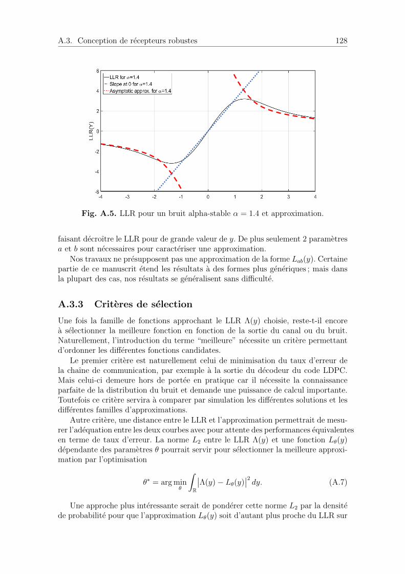
A.3. Conception de recepteurs robustes 128
Fig. A.5. LLR pour un bruit alpha-stable α = 1.4 et approximation.
faisant decroıtre le LLR pour de grande valeur de y. De plus seulement 2 parametresa et b sont necessaires pour caracteriser une approximation.
Nos travaux ne presupposent pas une approximation de la forme Lab(y). Certainepartie de ce manuscrit etend les resultats a des formes plus generiques ; mais dansla plupart des cas, nos resultats se generalisent sans difficulte.
A.3.3 Criteres de selection
Une fois la famille de fonctions approchant le LLR Λ(y) choisie, reste-t-il encorea selectionner la meilleure fonction en fonction de la sortie du canal ou du bruit.Naturellement, l’introduction du terme “meilleure” necessite un critere permettantd’ordonner les differentes fonctions candidates.
Le premier critere est naturellement celui de minimisation du taux d’erreur dela chaıne de communication, par exemple a la sortie du decodeur du code LDPC.Mais celui-ci demeure hors de portee en pratique car il necessite la connaissanceparfaite de la distribution du bruit et demande une puissance de calcul importante.Toutefois ce critere servira a comparer par simulation les differentes solutions et lesdifferentes familles d’approximations.
Autre critere, une distance entre le LLR et l’approximation permettrait de mesu-rer l’adequation entre les deux courbes avec pour attente des performances equivalentesen terme de taux d’erreur. La norme L2 entre le LLR Λ(y) et une fonction Lθ(y)dependante des parametres θ pourrait servir pour selectionner la meilleure approxi-mation par l’optimisation
θ∗ = arg minθ
∫R
∣∣Λ(y)− Lθ(y)∣∣2 dy. (A.7)
Une approche plus interessante serait de ponderer cette norme L2 par la densitede probabilite pour que l’approximation Lθ(y) soit d’autant plus proche du LLR sur
129 ANNEXE A. RESUME DETAILLE EN FRANCAIS
les domaines frequents de la sortie du canal, c’est-a-dire,
θ∗ = arg minθ
∫R
∣∣Λ(y)− Lθ(y)∣∣2 p(y) dy. (A.8)
Nous avons montre dans [MSG+19a] que ce critere permet de borner la divergencede Kullback-Leibler entre l’a posteriori Pr[X = x|Y = y] et son approximationPrθ[X = x|Y = y] obtenue en remplacant Λ(y) par Lθ(y) dans (A.5),
KEQM ≤ D(
Prθ[X = x|Y = y]∥∥∥Pr[X = x|Y = y]
)≤ K ′EQM, (A.9)
ou sont EQM, pour erreur quadratique moyenne, est la norme ponderee ou (A.8) etou K et K ′ deux constantes. Ainsi la selection par le critere EQM est proche en uncertain sens d’une selection par une recherche de probabilite la plus proche de l’aposteriori. selon une approche variationnelle.
Le dernier critere qui est a la base de l’approche que nous developperons parla suite repose sur la theorie de l’information et notamment sur l’idee presenteedans [YA09]. La capacite d’un canal MBISO s’ecrit comme C = H(X) −H(X|Y ).Or, d’une part, par equiprobabilite de l’entree binaire, H(X) = 1 et comme d’autrepart, la loi de X|Y est donnee par (A.5),
C = 1− E log2
(1 + e−XΛ(Y )
). (A.10)
Il est possible de borner inferieurement la capacite C par une valeur approcheeCθ obtenue en remplacant comme ci-dessus le LLR Λ(y) par une fonction approcheeLθ(y),
C ≥ Cθ = 1− E log2
(1 + e−XLθ(Y )
). (A.11)
Le critere de selection devient ici
θ∗ = arg maxθ
1− E log2
(1 + e−XLθ(Y )
), (A.12)
ou, de facon equivalente,
θ∗ = arg minθHθ(X|Y ) avec Hθ(X|Y ) = E log2
(1 + e−XLθ(Y )
). (A.13)
Le critere (A.13) est pertinent car l’ecart entre C et Cθ vaut la divergencede Kullback-Leibler entre l’a posteriori Pr θ[X = x|Y = y] et son approximationPrθ[X = x|Y = y].
A.4 Apprentissage supervise du LLR
Le critere de selection d’une fonction approchant le LLR dans une famille parametreeest maintenant fourni par (A.13). Il n’est pas utilisable tel quel car il fait intervenirl’esperance mathematique sur X et sur Y . Nous proposons et etudions par la suiteune methode d’optimisation de ce critere utilisable dans une chaıne de communica-tions.
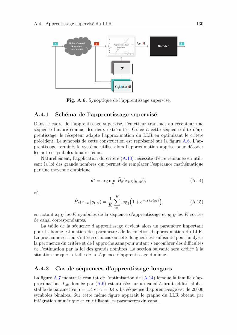
A.4. Apprentissage supervise du LLR 130
𝜽∗
𝑪𝑳𝜽[𝑿;𝑳𝜽(𝐘)]
Noise Channel N = noise +
Interference
YX 𝑿Decoder
Approximated LLR Estimator
𝐿𝜽∗ (Y)
Fig. A.6. Synoptique de l’apprentissage supervise.
A.4.1 Schema de l’apprentissage supervise
Dans le cadre de l’apprentissage supervise, l’emetteur transmet au recepteur unesequence binaire connue des deux extremites. Grace a cette sequence dite d’ap-prentissage, le recepteur adapte l’approximation du LLR en optimisant le critereprecedent. Le synopsis de cette construction est represente sur la figure A.6. L’ap-prentissage termine, le systeme utilise alors l’approximation apprise pour decoderles autres symboles binaires emis.
Naturellement, l’application du critere (A.13) necessite d’etre remaniee en utili-sant la loi des grands nombres qui permet de remplacer l’esperance mathematiquepar une moyenne empirique
θ∗ = arg minθHθ(x1:K |y1:K), (A.14)
ou
Hθ(x1:K |y1:K) =1
K
K∑i=1
log2
(1 + e−xkLθ(yk)
), (A.15)
en notant x1:K les K symboles de la sequence d’apprentissage et y1:K les K sortiesde canal correspondantes.
La taille de la sequence d’apprentissage devient alors un parametre importantpour la bonne estimation des parametres de la fonction d’approximation du LLR.La prochaine section s’interesse au cas ou cette longueur est suffisante pour analyserla pertinence du critere et de l’approche sans pour autant s’encombrer des difficultesde l’estimation par la loi des grands nombres. La section suivante sera dediee a lasituation lorsque la taille de la sequence d’apprentissage diminue.
A.4.2 Cas de sequences d’apprentissage longues
La figure A.7 montre le resultat de l’optimisation de (A.14) lorsque la famille d’ap-proximations Lab donnee par (A.6) est utilisee sur un canal a bruit additif alpha-stable de parametres α = 1.4 et γ = 0.45. La sequence d’apprentissage est de 20000symboles binaires. Sur cette meme figure apparaıt le graphe du LLR obtenu parintegration numerique et en utilisant les parametres du canal.
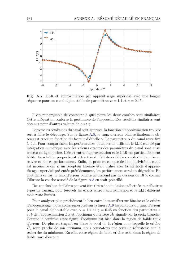
131 ANNEXE A. RESUME DETAILLE EN FRANCAIS
Fig. A.7. LLR et approximation par apprentissage supervise avec une longuesequence pour un canal alpha-stable de parametres α = 1.4 et γ = 0.45.
Il est remarquable de constater a quel point les deux courbes sont similaires.Cette adequation conforte la pertinence de l’approche. Des resultats similaires sontobtenus pour d’autres valeurs de α et γ.
Lorsque les conditions du canal sont apprises, la fonction d’approximation trouveesert a faire le decodage. Sur la figure A.8, le taux d’erreur binaire finalement ob-tenu est trace en fonction du facteur d’echelle γ. Le parametre α du canal reste fixea 1.4. Pour comparaison, les performances obtenues en utilisant le LLR calcule parintegration numerique avec les valeurs exactes des parametres du canal sont aussitracees en ligne pleine. L’ecart entre l’approximation et le LLR est particulierementfaible. La solution proposee est attractive du fait de sa faible complexite de mise enœuvre et de ses performances. Enfin, la prise en compte de l’impulsivite du canalest necessaire car si un recepteur lineaire etait utilise avec la methode d’appren-tissage supervise presentee precedemment, les performances seraient degradees. Eneffet dans ce cas, le taux d’erreur binaire ne descend pas en dessous de 10 % commel’illustre la courbe associe de la figure A.8 en trait pointille.
Des conclusions similaires peuvent etre tirees de simulations effectuees sur d’autrestypes de canaux, pour lesquels les ecarts entre l’approximation et le LLR differentmais reste limites.
Pour analyser plus precisement le lien entre le taux d’erreur binaire et le critered’apprentissage, nous avons superpose sur la figure A.9 les contours du taux d’erreurpour le canal alpha-stable avec α = 1.4 et γ = 0.45 en fonction des parametres aet b de l’approximation Lab et l’optimum du critere Hθ signale par la croix blanche.Comme le confirme cette figure, l’optimum est bien dans la region de faible tauxd’erreur. De plus en tracant en blanc le bord de la region pour laquelle le critereHθ reste proche de son optimum, nous constatons une certaine robustesse sur larecherche du minimum. En effet cette region de faible critere reste dans la region defaible taux d’erreur.

A.4. Apprentissage supervise du LLR 132
Fig. A.8. Taux d’erreur apres decodage utilisant l’approximation du LLR, le LLRou une approximation lineaire avec un canal alpha-stable d’exposant caracteristiqueα = 1.4.
10−5
10−4
10−3
10−2
10−1
𝟏𝟎−𝟓𝟏𝟎−𝟒
𝟏𝟎−𝟑
𝟏𝟎−𝟐
BER
Fig. A.9. Taux d’erreur binaire et critere Hθ.

133 ANNEXE A. RESUME DETAILLE EN FRANCAIS
Fig. A.10. Comparaison des familles Lab et Labc.
A.4.3 Une nouvelle famille d’approximations
Une analyse detaillee de l’approximation Lab nous a amene a ajouter un nouveauparametre c pour modeliser le passage de la partie lineaire a la partie asymptotique.La nouvelle famille Labc d’approximations est definie par
Labc(y) =
ay si −c/a < y < c/a,
c si c/a < y < bc,
b/y sinon.
(A.16)
La figure A.10 permet de comparer visuellement l’adequation entre le LLR, lameilleure fonction de type Lab et la meilleure de type Labc. L’ajout de ce parametrec permet de mieux prendre en compte la transition entre les deux regimes lineaireet asymptotique. Cela est particulierement important car cette zone represententenviron 40 % des sorties du canal qui sont par consequent mal pris en compte parl’approximation — la densite de la sortie du canal est aussi representee sur cettefigure.
Comme le montre la figure A.11, l’ecart de performance entre le LLR et l’op-timum des familles Lab est reduit par l’introduction de ce parametre c aussi bienpour le taux d’erreur binaire que pour le taux d’erreur paquet. Les conditions sontidentiques aux simulations de la figure A.8.
Nous resterons malgre cela sur la famille Lab par la suite pour rester sur uneoptimisation sur deux parametres.
A.4.4 Cas de sequence d’apprentissage courtes
Lorsque la sequence d’apprentissage devient plus courte, deux phenomenes appa-raissent. Le premier concerne l’estimation de Hθ par Hθ qui devient moins precise
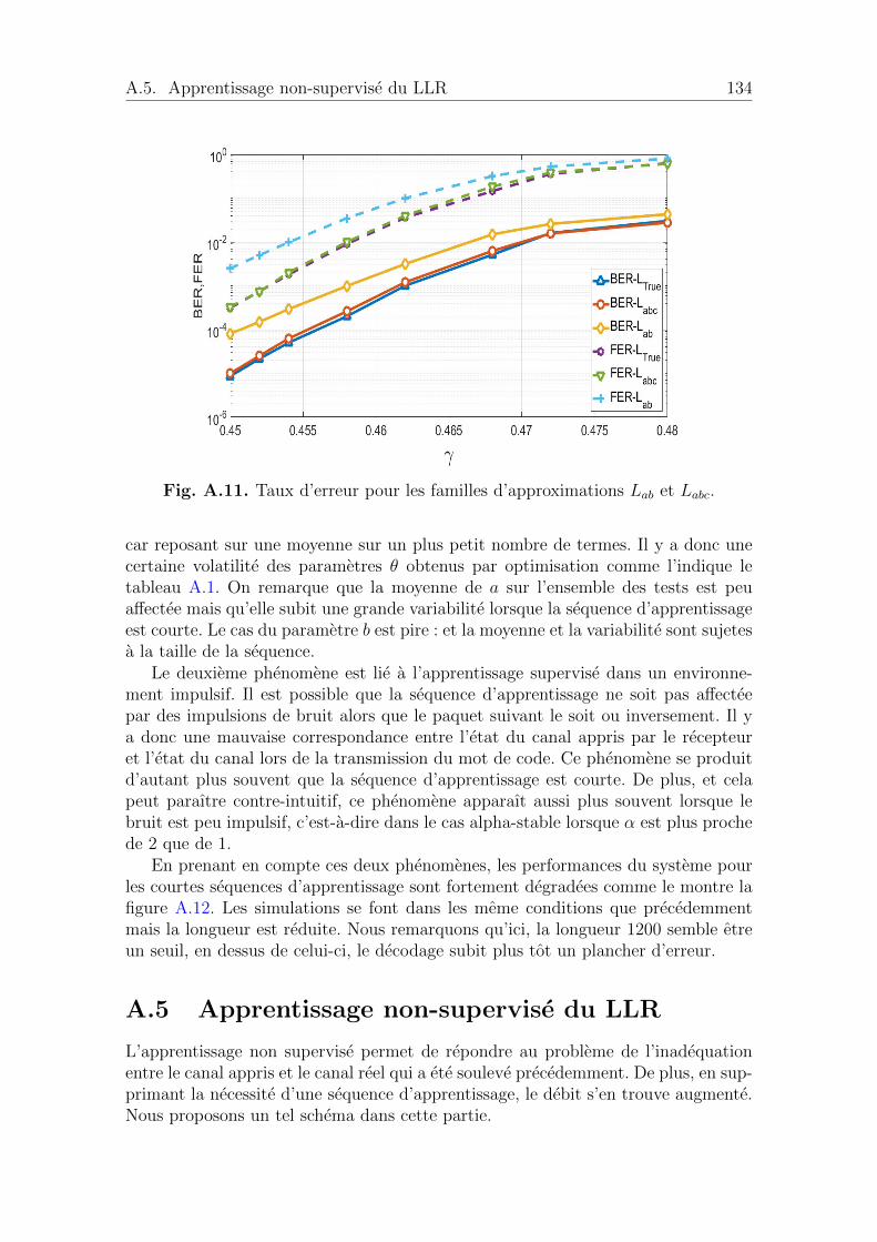
A.5. Apprentissage non-supervise du LLR 134
Fig. A.11. Taux d’erreur pour les familles d’approximations Lab et Labc.
car reposant sur une moyenne sur un plus petit nombre de termes. Il y a donc unecertaine volatilite des parametres θ obtenus par optimisation comme l’indique letableau A.1. On remarque que la moyenne de a sur l’ensemble des tests est peuaffectee mais qu’elle subit une grande variabilite lorsque la sequence d’apprentissageest courte. Le cas du parametre b est pire : et la moyenne et la variabilite sont sujetesa la taille de la sequence.
Le deuxieme phenomene est lie a l’apprentissage supervise dans un environne-ment impulsif. Il est possible que la sequence d’apprentissage ne soit pas affecteepar des impulsions de bruit alors que le paquet suivant le soit ou inversement. Il ya donc une mauvaise correspondance entre l’etat du canal appris par le recepteuret l’etat du canal lors de la transmission du mot de code. Ce phenomene se produitd’autant plus souvent que la sequence d’apprentissage est courte. De plus, et celapeut paraıtre contre-intuitif, ce phenomene apparaıt aussi plus souvent lorsque lebruit est peu impulsif, c’est-a-dire dans le cas alpha-stable lorsque α est plus prochede 2 que de 1.
En prenant en compte ces deux phenomenes, les performances du systeme pourles courtes sequences d’apprentissage sont fortement degradees comme le montre lafigure A.12. Les simulations se font dans les meme conditions que precedemmentmais la longueur est reduite. Nous remarquons qu’ici, la longueur 1200 semble etreun seuil, en dessus de celui-ci, le decodage subit plus tot un plancher d’erreur.
A.5 Apprentissage non-supervise du LLR
L’apprentissage non supervise permet de repondre au probleme de l’inadequationentre le canal appris et le canal reel qui a ete souleve precedemment. De plus, en sup-primant la necessite d’une sequence d’apprentissage, le debit s’en trouve augmente.Nous proposons un tel schema dans cette partie.
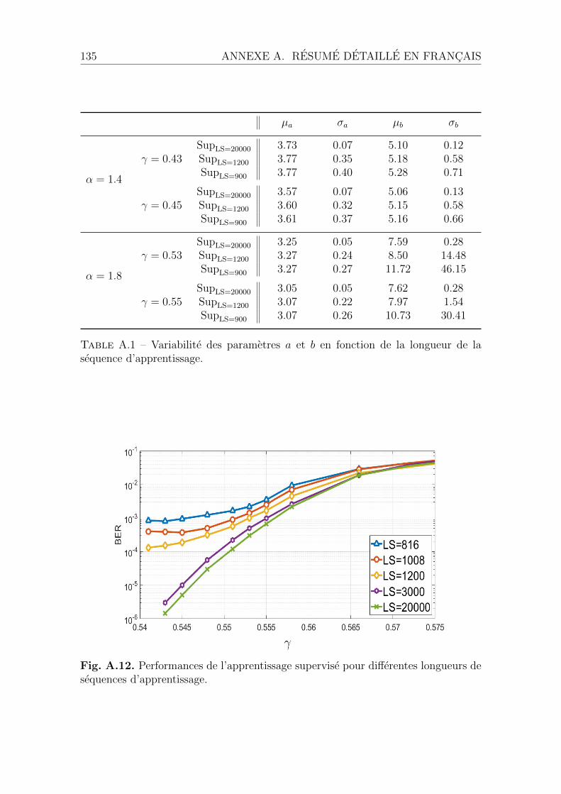
135 ANNEXE A. RESUME DETAILLE EN FRANCAIS
µa σa µb σb
α = 1.4
γ = 0.43SupLS=20000 3.73 0.07 5.10 0.12SupLS=1200 3.77 0.35 5.18 0.58SupLS=900 3.77 0.40 5.28 0.71
γ = 0.45SupLS=20000 3.57 0.07 5.06 0.13SupLS=1200 3.60 0.32 5.15 0.58SupLS=900 3.61 0.37 5.16 0.66
α = 1.8
γ = 0.53SupLS=20000 3.25 0.05 7.59 0.28SupLS=1200 3.27 0.24 8.50 14.48SupLS=900 3.27 0.27 11.72 46.15
γ = 0.55SupLS=20000 3.05 0.05 7.62 0.28SupLS=1200 3.07 0.22 7.97 1.54SupLS=900 3.07 0.26 10.73 30.41
Table A.1 – Variabilite des parametres a et b en fonction de la longueur de lasequence d’apprentissage.
Fig. A.12. Performances de l’apprentissage supervise pour differentes longueurs desequences d’apprentissage.

A.5. Apprentissage non-supervise du LLR 136
θ∗
I[෩𝑿 ;𝑳θ(෩𝒀)]
Noise Channel N = noise +
Interference
𝐿θ∗ (Y)
෩𝑵
෩𝑿
Approximated LLR Demapper
Decoder
෩𝒀
Simulated Channel
𝑎∗ 𝑏∗
Fig. A.13. Synopsis de l’apprentissage non-supervise.
A.5.1 Schema de l’apprentissage non-supervise
Notre methode cherche a reconstruire un canal equivalent avec une source connue durecepteur. Pour cela, le schema de la figure A.13 est utilise. Des echantillons de bruitsont d’abord extraits grace a une detection par le signe. Ensuite, ces echantillonsde bruit sont injectes dans un canal simule dont la pseudo-source est generee parle recepteur. Grace a cela, la methode precedente dite supervisee est utilisee pourestimer les parametres θ de l’approximation du LLR.
Meme si certaines decisions sont erronees, l’estimation obtenue pour a et bpeuvent etre suffisamment proche de l’optimum pour permettre un decodage per-formant. Deux cas sont a considerer : soit les codes sont longs soit ils sont courts.Les parties suivantes developpent ces cas.
A.5.2 Cas des paquets longs
La figure A.14 compare les parametres a et b dans le cadre d’un apprentissagesupervise et d’un apprentissage non-supervise avec une taille de sequence ou de motde code de 20000. Le parametre a est peu affecte par les erreurs de decision duschema non-supervise contrairement au second parametre b. Toutefois les ordres degrandeurs de ce parametre ne sont pas aberrants ce qui presage d’une degradationlimitee des performances.
Comme le montre la figure A.15, en reprenant les memes parametres de simu-lations que pour le cas supervise, les performances de notre systeme non superviserestent proches du systeme supervise sur de longues sequences de taille 20000. Onremarque que ces performances sont meme superieures a un systeme supervise avecune sequence d’apprentissage de longueur 1200. Naturellement, l’ecart de perfor-mance entre le supervise et le non-supervise depend du canal mais reste cependantlimite.
A.5.3 Cas des paquets courts
Le cas des paquets courts en non-supervise est plus complexe a etudier car plu-sieurs phenomenes interviennent. Comme le montre la courbe legendee ” USD ”de la figure A.16, l’apprentissage ne parvient pas a approcher correctement le LLR
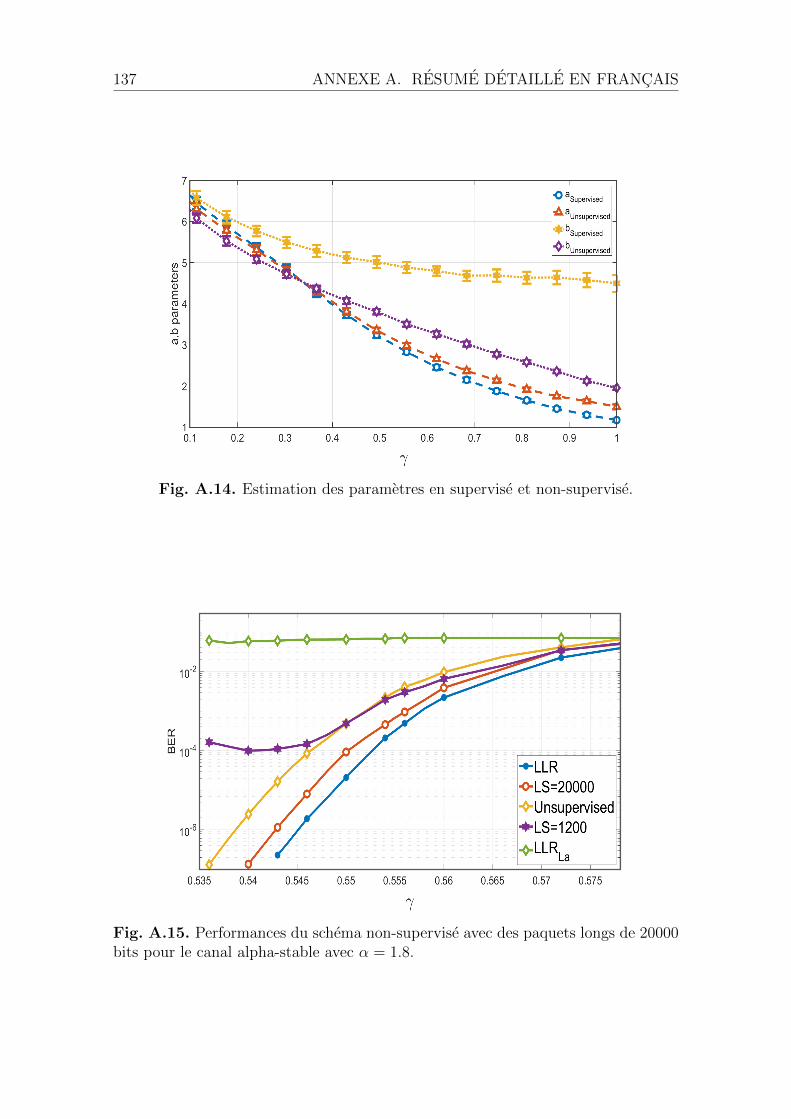
137 ANNEXE A. RESUME DETAILLE EN FRANCAIS
Fig. A.14. Estimation des parametres en supervise et non-supervise.
Fig. A.15. Performances du schema non-supervise avec des paquets longs de 20000bits pour le canal alpha-stable avec α = 1.8.

A.5. Apprentissage non-supervise du LLR 138
0.1 0.2 0.3 0.4 0.5 0.6 0.710-5
10-4
10-3
10-2
10-1
100
BE
R
OptimalGADUSD
old
Fig. A.16. Performances du schema non-supervise avec des paquets courts de 408bits sur un canal alpha-stable de parametre α = 1.8.
representee par la courbe legendee ” Optimal”. De plus, un sursaut d’erreurs ap-paraıt quand bien meme le bruit est plus faible.
Pour comprendre les raisons de ce comportement, un schema qualifie de GADpour Genie Aided Decoder est utilise. Il utilise le meme schema que l’apprentissagenon-supervise mais ou l’entree estimee X est remplacee par les bits reellement emisX. Les performances du schema GAD sont quasiment indiscernables de l’optimal.
Une etude fine permet de constater que les parametres a et b deviennent hau-tement variables en fonction des conditions du canal. Par consequent, le LLR estrarement correctement approche par la fonction Lab. Cette variabilite s’explique parune degenerescence du processus optimisation. En effet, le critere (A.15) exprimeun compromis entre quatre termes : l’un tend a faire augmenter le parametre a tan-dis que l’autre tend a l’annuler, les deux autres termes jouent des roles identiquesavec le parametre b. Il y a degenerescence si l’un de ces quatre termes disparaıtfaute d’echantillon de bruit associe. Dans ce cas, l’un des parametres a ou b devientsoit infini soit nul ce que rend l’approximation du LLR inoperante et explique ladegradation des performances.
Nous avons quantifie theoriquement le risque d’apparition d’une degenerescence.La figure A.17 en trace les valeurs. L’apprentissage non-supervise presente un risqueaccru de degenerescence par rapport au GAD. Et cette difference est la plus grandejustement dans la zone de bruit ou un sursaut d’erreur est observee dans la fi-gure A.16.
Pour corriger ces problemes de l’apprentissage non-supervise pour les paquetscourts, nous avons alors propose une solution simple. Le resultat se retrouve sur lafigure A.18 sous la legende USDnew. La solution proposee permet de retrouver desperformances proche de l’optimum du LLR.
Cette correction consiste a symetriser la distribution des echantillons de bruit

139 ANNEXE A. RESUME DETAILLE EN FRANCAIS
.
0.1 0.2 0.3 0.4 0.5 0.6 0.7 0.8
2
0.82
0.84
0.86
0.88
0.9
0.92
0.94
0.96
0.98
USD, ,=1.8GAD, ,=1.8USD, ,=1.4GAD, ,=1.4
1
Fig. A.17. Risque de degenerescence en fonction de γ pour un canal alpha-stable.
0.1 0.2 0.3 0.4 0.5 0.6 0.7
10-6
10-4
10-2
100
BER
OptimalGADUSD
new
USDold
Fig. A.18. Performances de l’apprentissage supervisee corrige.

A.5. Apprentissage non-supervise du LLR 140
reconstitues puis a introduire un terme de regulation sur le parametre a critere Hθ
qui est equivalent a ajouter un echantillon de bruit faible est negatif. Cette solutiona quasiment aucun cout de calcul supplementaire par rapport a la version originaleet pourtant ses performances sont satisfaisantes.
A.5.4 Conclusion et perspectives
Nous avons montre dans nos travaux qu’un simple module entre la sortie du canalet l’entree du decodeur de canal permet de combattre efficacement le bruit et lesinterferences qui perturbent les communications point a point dans un reseau. Cemodule consiste en un fonction approchant le calcul du rapport de vraisemblancequi est rarement accessible et qui necessite la connaissance de l’etat du canal. Or,grace a un critere judicieux, il est possible de chercher cette fonction d’approximationefficacement soit par un apprentissage supervise soit par une approche non-supervise.Nous avons montre qu’il devient meme possible d’utiliser un tel schema pour descommunications par paquets courts sans pertes redhibitoires de performances.
Les perspectives de nos travaux sont nombreux. La premiere, a court terme,consiste a etendre nos resultats pour des modulations d’ordre superieur comme lesmodulations d’amplitude en quadrature. Dans ce cas les rapports de vraisemblancesdependent de la position des bits dans le codage binaire des symboles. Il faut doncproposer des familles de fonctions approchantes qui prennent en compte cette po-sition. Toutefois, nos travaux preliminaires montrent qu’il est possible de revenir aun melange de nos fonctions Lab pour limiter la taille des parametres.
A plus long terme, comme le critere propose est tres proche d’une approchevariationnelle de l’apprentissage, il peut etre judicieux de l’integrer directement dansle decodage canal pour qu’il y ait un echange d’information entre le code et le calculdu LLR. Cela est d’autant plus pertinent que dans le cas non-supervise, la limitationdu nombre d’erreurs de decision ameliore la qualite des echantillons de bruit obtenuset donc de l’estimation des parametres. Un couplage simple entre le decodage decanal et l’approximation a deja ete teste sans resultat significatif ce qui incite arechercher une approche plus fine, par exemple par l’utilisation d’un couplage degraphes factoriels entre celui du code LDPC et celui de l’approximation du LLR.
Enfin, nous avons toujours considere des approximations qui appartiennent a unecertaine famille construite a priori. Le critere etant issu de la theorie de l’information,il serait profitable de rendre l’approche encore plus generique en choisissant unefonction selon une approche par maximum d’entropie a la Jaynes [Jay03] et en lacombinant avec le decodage de canal directement pour faire un decodeur base sur leprincipe du maximum d’entropie.
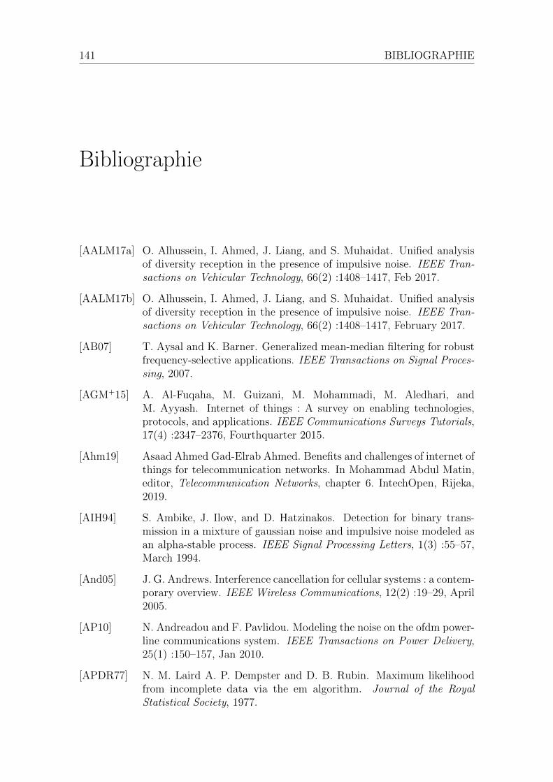
141 BIBLIOGRAPHIE
Bibliographie
[AALM17a] O. Alhussein, I. Ahmed, J. Liang, and S. Muhaidat. Unified analysisof diversity reception in the presence of impulsive noise. IEEE Tran-sactions on Vehicular Technology, 66(2) :1408–1417, Feb 2017.
[AALM17b] O. Alhussein, I. Ahmed, J. Liang, and S. Muhaidat. Unified analysisof diversity reception in the presence of impulsive noise. IEEE Tran-sactions on Vehicular Technology, 66(2) :1408–1417, February 2017.
[AB07] T. Aysal and K. Barner. Generalized mean-median filtering for robustfrequency-selective applications. IEEE Transactions on Signal Proces-sing, 2007.
[AGM+15] A. Al-Fuqaha, M. Guizani, M. Mohammadi, M. Aledhari, andM. Ayyash. Internet of things : A survey on enabling technologies,protocols, and applications. IEEE Communications Surveys Tutorials,17(4) :2347–2376, Fourthquarter 2015.
[Ahm19] Asaad Ahmed Gad-Elrab Ahmed. Benefits and challenges of internet ofthings for telecommunication networks. In Mohammad Abdul Matin,editor, Telecommunication Networks, chapter 6. IntechOpen, Rijeka,2019.
[AIH94] S. Ambike, J. Ilow, and D. Hatzinakos. Detection for binary trans-mission in a mixture of gaussian noise and impulsive noise modeled asan alpha-stable process. IEEE Signal Processing Letters, 1(3) :55–57,March 1994.
[And05] J. G. Andrews. Interference cancellation for cellular systems : a contem-porary overview. IEEE Wireless Communications, 12(2) :19–29, April2005.
[AP10] N. Andreadou and F. Pavlidou. Modeling the noise on the ofdm power-line communications system. IEEE Transactions on Power Delivery,25(1) :150–157, Jan 2010.
[APDR77] N. M. Laird A. P. Dempster and D. B. Rubin. Maximum likelihoodfrom incomplete data via the em algorithm. Journal of the RoyalStatistical Society, 1977.
Bibliographie 142
[AWM14] A. Asadi, Q. Wang, and V. Mancuso. A survey on device-to-devicecommunication in cellular networks. IEEE Communications SurveysTutorials, 16(4) :1801–1819, Fourthquarter 2014.
[BALE+07] Torben Brack, M. Alles, Timo Lehnigk-Emden, F. Kienle, NorbertWehn, N.E. L’Insalata, F. Rossi, Massimo Rovini, and Luca Fanucci.Low complexity ldpc code decoders for next generation standards. 2008Design, Automation and Test in Europe, 0 :69, 04 2007.
[BD03] L. Barnault and D. Declercq. Fast decoding algorithm for ldpc overgf(2/sup q/). In Proceedings 2003 IEEE Information Theory Workshop(Cat. No.03EX674), pages 70–73, March 2003.
[BEK98] Franco Bassi, Paul Embrechts, and Maria Kafetzaki. A Practical Guideto Heavy Tails. Birkhauser Boston Inc., Cambridge, MA, USA, 1998.
[BMA10] H. Bhaskar, L. Mihaylova, and A. Achim. Video foreground detectionbased on symmetric alpha-stable mixture models. IEEE Trans. Cir.and Sys. for Video Technol., 20(8) :1133–1138, August 2010.
[BMR+13] R. Bassoli, H. Marques, J. Rodriguez, K. W. Shum, and R. Tafazolli.Network coding theory : A survey. IEEE Communications SurveysTutorials, 15(4) :1950–1978, Fourth 2013.
[BN10] N. C. Beaulieu and S. Niranjayan. Uwb receiver designs based on agaussian-laplacian noise-plus-mai model. IEEE Transactions on Com-munications, 58(3) :997–1006, March 2010.
[BRB93] K. L. Blackard, T. S. Rappaport, and C. W. Bostian. Measurementsand models of radio frequency impulsive noise for indoor wireless com-munications. IEEE Journal on Selected Areas in Communications,11(7) :991–1001, Sep. 1993.
[BSE10] A. Skrondal B. S. Everitt. The Cambridge dictionary of Statistics.Fourth Edition Cambridge university press, 2010.
[BSF08] N. C. Beaulieu, Hua Shao, and J. Fiorina. P-order metric UWB re-ceiver structures with superior performance. IEEE Transactions onCommunications, 56(10) :1666–1676, October 2008.
[BY09] N. C. Beaulieu and D. J. Young. Designing time-hopping ultrawidebandwidth receivers for multiuser interference environments. Procee-dings of the IEEE, 97(2) :255–284, Feb 2009.
[CAG08] V. Chandrasekhar, J. G. Andrews, and A. Gatherer. Femtocell net-works : a survey. IEEE Communications Magazine, 46(9) :59–67, Sep.2008.
[Car10] P. Cardieri. Modeling interference in wireless Ad Hoc networks. IEEECommunications Surveys Tutorials, 12(4) :551–572, Fourth 2010.
143 BIBLIOGRAPHIE
[CBV+09] N. Czink, B. Bandemer, G. Vazquez-Vilar, L. Jalloul, C. Oestges, andA. Paulraj. Spatial separation of multi-user mimo channels. In 2009IEEE 20th International Symposium on Personal, Indoor and MobileRadio Communications, pages 1059–1063, Sep. 2009.
[CGE+09] A. Chopra, K. Gulati, B. L. Evans, K. R. Tinsley, and C. Sreerama.Performance bounds of mimo receivers in the presence of radio fre-quency interference. In 2009 IEEE International Conference on Acous-tics, Speech and Signal Processing, pages 2817–2820, April 2009.
[Chu05] T. C. Chuah. Robust iterative decoding of turbo codes in heavy-tailednoise. IEE Proceedings - Communications, 152(1) :29–38, Feb 2005.
[CL97] R. C. Cheng and W. Liu. A continuous representation of the familyof stable law distributions. Journal of the Royal Statistical Society :Series B (Statistical Methodology), pages 137–145, 1997.
[CLCC11] S. Cheng, S. Lien, F. Chu, and K. Chen. On exploiting cognitive radioto mitigate interference in macro/femto heterogeneous networks. IEEEWireless Communications, 18(3) :40–47, June 2011.
[Coo93] John W. Cook. Wideband impulsive noise survey of the access network.1993.
[Cos83] M. Costa. Writing on dirty paper (corresp.). IEEE Transactions onInformation Theory, 29(3) :439–441, May 1983.
[CPH04] M. Chitre, J. Potter, and O. S. Heng. Underwater acoustic chan-nel characterisation for medium-range shallow water communica-tions. In Oceans ’04 MTS/IEEE Techno-Ocean ’04 (IEEE Cat.No.04CH37600), volume 1, pages 40–45 Vol.1, Nov 2004.
[CT06] Thomas M. Cover and Joy A. Thomas. Elements of InformationTheory. Wiley, 2 edition, 2006.
[CTB98] Mark E. Crovella, Murad S. Taqqu, and Azer Bestavros. A PracticalGuide to Heavy Tails. Birkhauser Boston Inc., Cambridge, MA, USA,1998.
[DF07] D. Declercq and M. Fossorier. Decoding algorithms for nonbinary ldpccodes over gf(q). IEEE Transactions on Communications, 55(4) :633–643, April 2007.
[DGCG14] V. Dimanche, A. Goupil, L. Clavier, and G. Gelle. On detection me-thod for soft iterative decoding in the presence of impulsive interfe-rence. IEEE Communications Letters, 18(6) :945–948, June 2014.
[DHB06] J. Dielissen, A. Hekstra, and V. Berg. Low cost ldpc decoder for dvb-s2.In Proceedings of the Design Automation Test in Europe Conference,volume 2, pages 1–6, March 2006.
Bibliographie 144
[Dig09] Digi. Efficient data transfer over cellular networks. White Paper, 2009.
[DM98] M. C. Davey and D. J. C. MacKay. Low density parity check codesover gf(q). In 1998 Information Theory Workshop (Cat. No.98EX131),pages 70–71, June 1998.
[DuM73] William H. DuMouchel. On the asymptotic normality of the maximum-likelihood estimate when sampling from a stable distribution. Ann.Statist., 1(5) :948–957, 09 1973.
[Dur10] R. Durrett. Probability : Theory and Examples. 4th edition CambridgeSeries in Statistical and Probabilistic Mathematics, 2010.
[DYZB03] Duc Son Pham, Yee Hong Leung, A. Zoubir, and R. Brcic. On thecomputational aspect of robust multiuser detection. In Proceedingsof the 3rd IEEE International Symposium on Signal Processing andInformation Technology (IEEE Cat. No.03EX795), pages 22–25, Dec2003.
[ECD08] T. Erseghe, V. Cellini, and G. Dona. On uwb impulse radio receiversderived by modeling mai as a gaussian mixture process. IEEE Tran-sactions on Wireless Communications, 7(6) :2388–2396, June 2008.
[ECdF+17] M. Egan, L. Clavier, M. de Freitas, L. Dorville, J.M. Gorce, and A. Sa-vard. Wireless communication in dynamic interference. In IEEE GLO-BECOM, Singapore, December 2017.
[ECZ+18] Malcolm Egan, Laurent Clavier, Ce Zheng, Mauro de Freitas, and Jean-Marie Gorce. Dynamic interference for uplink scma in large-scale wi-reless networks without coordination. EURASIP Journal on WirelessCommunications and Networking, 2018(1) :213, Aug 2018.
[EPH13] O. El Ayach, S. W. Peters, and R. W. Heath. The practical challengesof interference alignment. IEEE Wireless Communications, 20(1) :35–42, February 2013.
[ETV99] T. Etzion, A. Trachtenberg, and A. Vardy. Which codes have cycle-free tanner graphs ? IEEE Transactions on Information Theory,45(6) :2173–2181, Sep. 1999.
[FC09] D. Fertonani and G. Colavolpe. A robust metric for soft-output detec-tion in the presence of class-A noise. IEEE Transactions on Commu-nications, 57(1) :36–40, January 2009.
[Fel70] W. Feller. An Introduction to Probability Theory and its Applications,volume I of Wiley Series in Probability and Mathematical Statistics.John Wiley & Sons, New York, 1970.
[FGCE15] N. Farsad, W. Guo, C. Chae, and A. Eckford. Stable distributionsas noise models for molecular communication. In 2015 IEEE GlobalCommunications Conference (GLOBECOM), pages 1–6, Dec 2015.

145 BIBLIOGRAPHIE
[Fio06] J. Fiorina. Wlc28-2 : A simple ir-uwb receiver adapted to multi-userinterferences. In IEEE Globecom 2006, pages 1–4, Nov 2006.
[FR71] Eugene F. Fama and Richard Roll. Parameter estimates for symmetricstable distributions. Journal of the American Statistical Association,66(334) :331–338, 1971.
[Gal63] Robert G. Gallager. Low density parity check codes. M.I.T press, 1963.
[GC12] W. Gu and L. Clavier. Decoding metric study for turbo codes in veryimpulsive environment. IEEE Communications Letters, 16(2) :256–258, February 2012.
[GCA+10] H. E. Ghannudi, L. Clavier, N. Azzaoui, F. Septier, and P. a. Rolland.α-stable interference modeling and cauchy receiver for an IR-UWB AdHoc network. IEEE Transactions on Communications, 58(6) :1748–1757, June 2010.
[GCGD07] A. Goupil, M. Colas, G. Gelle, and D. Declercq. Fft-based bp deco-ding of general ldpc codes over abelian groups. IEEE Transactions onCommunications, 55(4) :644–649, April 2007.
[GDK06] N. Guney, H. Delic, and M. Koca. Robust detection of ultra-widebandsignals in non-gaussian noise. IEEE Transactions on MicrowaveTheory and Techniques, 54(4) :1724–1730, June 2006.
[GEAT10] K. Gulati, B. L. Evans, J. G. Andrews, and K. R. Tinsley. Statistics ofco-channel interference in a field of poisson and poisson-poisson cluste-red interferers. IEEE Transactions on Signal Processing, 58(12) :6207–6222, Dec 2010.
[GH97] Jaap Geluk and Laurens Haan. Stable probability distributions andtheir domains of attraction. Tinbergen Institute, Tinbergen InstituteDiscussion Papers, 20, 01 1997.
[Gol05] A. Goldsmith. Wireless communications. Cambridge university press,2005.
[Gon97] J. G. Gonzalez. Robust techniques for wireless communications in non-Gaussian environments. PhD thesis, Dept. Elec. Eng., Univ. of Dela-ware, Newark, DE,, 1997.
[GPA06] J. Gonzalez, J. L. Paredes, and G. R. Arce. Zero-order statistics : A ma-thematical framework for the processing and characterization of veryimpulsive signals. IEEE Transactions on Signal Processing, 54 :3839–3851, 2006.
[GPC+12] W. Gu, G. Peters, L. Clavier, F. Septier, and I. Nevat. Receiver studyfor cooperative communications in convolved additive alpha-stable in-terference plus gaussian thermal noise. In 2012 International Sympo-sium on Wireless Communication Systems (ISWCS), pages 451–455,Aug 2012.
Bibliographie 146
[GSY09] X. Guo, H. Sun, and Yilong Lu. Joint suppression of radio frequencyinterference and lightning impulsive noise in hfswr. In 2009 Interna-tional Radar Conference ”Surveillance for a Safer World” (RADAR2009), pages 1–6, Oct 2009.
[Hag04] J. Hagenauer. The exit chart - introduction to extrinsic informationtransfer in iterative processing. In 2004 12th European Signal Proces-sing Conference, pages 1541–1548, Sep. 2004.
[Hal66] Harry Hall. A new model for impulsive phenomena : Application toatmospheric noise communication channels. page 179, 08 1966.
[HEg07] P.A. Rolland H. El ghannudi, L. Clavier. ”modelisation du maid’un systeme ir-uwb transpose a 60 ghz pour des reseaux ad hoc”modelisation du mai d’un systeme ir-uwb transpose a 60 ghz pour desreseaux ad hoc. GRETSI, 2007.
[HGC06] T. R. Halford, A. J. Grant, and K. M. Chugg. Which codes have4-cycle-free tanner graphs ? IEEE Transactions on Information Theory,52(9) :4219–4223, Sep. 2006.
[HH-56] An investigation of atmospheric radio noise at very low frequencies,volume 103. Proceedings of the IET, 1956.
[HLZ14] Y. Hou, R. Liu, and L. Zhao. A non-linear LLR approximation forLDPC decoding over impulsive noise channels. In 2014 IEEE/CICInternational Conference on Communications in China (ICCC), pages86–90, Oct 2014.
[HM12] J. Hoadley and P. Maveddat. Enabling small cell deployment withhetnet. IEEE Wireless Communications, 19(2) :4–5, April 2012.
[HSSL11] Y. Hao, Z. Shan, F. Shen, and D. Lv. Parameter estimation of alpha-stable distributions based on mcmc. In 2011 3rd International Confe-rence on Advanced Computer Control, pages 325–327, Jan 2011.
[IH98a] J. Ilow and D. Hatzinakos. Analytic alpha-stable noise modeling in apoisson field of interferers or scatterers. IEEE Transactions on SignalProcessing, 46(6) :1601–1611, June 1998.
[IH98b] J. Ilow and D. Hatzinakos. Analytic alpha-stable noise modeling in apoisson field of interferers or scatterers. IEEE Transactions on SignalProcessing, 46(6) :1601–1611, June 1998.
[III07] H. Ishikawa, M. Itami, and K. Itoh. A study on adaptive modulation ofofdm under middleton’s class-a impulsive noise model. In 2007 Digestof Technical Papers International Conference on Consumer Electro-nics, pages 1–2, Jan 2007.
[Jay03] E. T. Jaynes. Probability Theory : The Logic of Science. CambridgeUniversity Press, 2003.
147 BIBLIOGRAPHIE
[JG12] Sang-Woon Jeon and Michael Gastpar. A survey on interference net-works : Interference alignment and neutralization. Entropy, 14(10) :22.1842–1863, 2012.
[JHMB05] Kyle Jamieson, Bret Hull, Allen Miu, and Hari Balakrishnan. Unders-tanding the real-world performance of carrier sense. In Proceedingsof the 2005 ACM SIGCOMM Workshop on Experimental Approachesto Wireless Network Design and Analysis, E-WIND ’05, pages 52–57,New York, NY, USA, 2005. ACM.
[Joh08] S. J. Johnson. Iterative error correction : turbo, low-density parity-check and repeat-accumulate codes. Cambridge University Press, 2008.
[K60] G. Hagstroem K. Remarks on pareto distributions. Scandinavian Ac-tuarial Journal, 1960(1-2) :59–71, 1960.
[Kas88] S. A. Kassam. Signal Detection in Non-Gaussian Noise. Springer-Verlag, 1988.
[KC04] M. Karkooti and J. R. Cavallaro. Semi-parallel reconfigurable archi-tectures for real-time ldpc decoding. In International Conference onInformation Technology : Coding and Computing, 2004. Proceedings.ITCC 2004., volume 1, pages 579–585 Vol.1, April 2004.
[KFR98] E. E. Kuruoglu, W. J. Fitzgerald, and P. J. W. Rayner. Near optimaldetection of signals in impulsive noise modeled with a symmetric /splalpha/-stable distribution. IEEE Communications Letters, 2(10) :282–284, Oct 1998.
[KG95] K. J. Kerpez and A. M. Gottlieb. The error performance of digitalsubscriber lines in the presence of impulse noise. IEEE Transactionson Communications, 43(5) :1902–1905, May 1995.
[KH01] A. Karasaridis and D. Hatzinakos. Network heavy traffic modelingusing alpha-stable self-similar processes. IEEE Transaction on Com-munication, 2001.
[Kou81] Ioannis A. Koutrouvelis. An iterative procedure for the estimation ofthe parameters of stable laws. Communications in Statistics - Simula-tion and Computation, 10(1) :17–28, 1981.
[KTH95] S. Kuramoto, F. Takemoto, and M. Hattori. A study of impulse noisecaused by connecting or disconnecting coaxial cable between equip-ment. In Proceedings of International Symposium on ElectromagneticCompatibility, pages 501–506, Aug 1995.
[KTMP03] Koay Teong Beng, Tan Eng Teck, Mandar Chitre, and J. R. Potter.Estimating the spatial and temporal distribution of snapping shrimpusing a portable, broadband 3-dimensional acoustic array. In Oceans2003. Celebrating the Past ... Teaming Toward the Future (IEEE Cat.No.03CH37492), volume 5, pages 2706–2713 Vol.5, Sep. 2003.

Bibliographie 148
[Leg09] M. W. Legg. Non-Gaussian and non-homogeneous Poisson models ofsnapping shrimp noise. PhD thesis, Curtin University of Technology,2009.
[Mau16] Robert G Maunder. A vision for 5g channel coding. AccelerCommWhite Paper, October 2016.
[McC86a] J. H. McCulloch. Simple consistent estimators of stable distributionparameters. Communications on Satatistical Simulations, pages 1109–1136, 1986.
[McC86b] J. Huston McCulloch. Simple consistent estimators of stable distri-bution parameters. Communications in Statistics - Simulation andComputation, 15(4) :1109–1136, 1986.
[MGC05] H. Meng, Y. L. Guan, and S. Chen. Modeling and analysis of noiseeffects on broadband power-line communications. IEEE Transactionson Power Delivery, 20(2) :630–637, April 2005.
[MGCG10a] H. Ben Maad, A. Goupil, L. Clavier, and G. Gelle. Asymptotic perfor-mance of ldpc codes in impulsive non-gaussian channel. In Signal Pro-cessing Advances in Wireless Communications (SPAWC), 2010 IEEEEleventh International Workshop on, pages 1–5, June 2010.
[MGCG10b] H. Ben Maad, A. Goupil, L. Clavier, and G. Gelle. Robust clippingdemapper for LDPC decoding in impulsive channel. In 2010 6th Inter-national Symposium on Turbo Codes Iterative Information Processing,pages 231–235, Sept 2010.
[MGCG13] H. B. Maad, A. Goupil, L. Clavier, and G. Gelle. Clipping demapper forLDPC decoding in impulsive channel. IEEE Communications Letters,17(5) :968–971, May 2013.
[Mid72a] D. Middleton. Performance of telecommunications systems in the spec-traluse environment : Vii. interference scenarios and the canonical andquasi-canonical (first-order) probability models of class a interference.1972.
[Mid72b] David Middleton. Statistical-physical models of urban radio-noise en-vironments - part i : Foundations. 1972.
[Mid77] D. Middleton. Statistical-physical models of electromagnetic interfe-rence. IEEE Transactions on Electromagnetic Compatibility, EMC-19(3) :106–127, August 1977.
[Mid96] D. Middleton. An Introduction to Statistical Communication Theory,chapter 11. IEEE, 1996.
[MJLC15] Z. Mei, M. Johnston, S. Le, and L. Chen. Density evolution analysisof LDPC codes with different receivers on impulsive noise channels.

149 BIBLIOGRAPHIE
In 2015 IEEE/CIC International Conference on Communications inChina (ICCC), pages 1–6, Nov 2015.
[MN96] D. J. C. MacKay and R. M. Neal. Near shannon limit performance oflow density parity check codes. Electronics Letters, 32(18) :1645–, Aug1996.
[MS02] M. M. Mansour and N. R. Shanbhag. Low-power vlsi decoder archi-tectures for ldpc codes. In Proceedings of the International Symposiumon Low Power Electronics and Design, pages 284–289, Aug 2002.
[MSG+18] Yasser Mestrah, Anne Savard, Alban Goupil, Laurent Clavier, andGuillaume Gelle. Blind estimation of an approximated likelihood ra-tio in impulsive environment. In IEEE International Symposium onPersonal, Indoor and Mobile Radio Communications, 2018.
[MSG+19a] Yasser Mestrah, Anne Savard, Alban Goupil, Guillaume Gelle, andLaurent Clavier. Mesure indirecte des performances de llr approche.In GRETSI, 2019.
[MSG+19b] Yasser Mestrah, Anne Savard, Alban Goupil, Guillaume Gelle, andLaurent Clavier. On unsupervised llr estimation under finite block-length with unknown noise distribution. To be published, 2019.
[MSG+19c] Yasser Mestrah, Anne Savard, Alban Goupil, Guillaume Gelle, andLaurent Clavier. Robust and simple log-likelihood approximation forreceiver design. In IEEE Wireless Communications and NetworkingConference (IEEE WCNC), 2019.
[MSG+19d] Yasser Mestrah, Anne Savard, Alban Goupil, Guillaume Gelle, andLaurent Clavier. An unsupervised llr estimation with unknown noisedistribution. EURASIP Journal on Wireless Communications andNetworking, 2019.
[MT76] J. H. Miller and J. B. Thomas. The detection of signals in impulsivenoise modeled as a mixture process. IEEE Trans. on Comm., 1976.
[Nah09] D. F. Nahimana. Impact des multi trajets sur les performances dessystemes de navigation par satellite : Contribution a l’amelioration dela precision de localisation par modelisation bayesienne. PhD thesis,Ecole centrale Lille, 2009.
[NB08] S. Niranjayan and N. C. Beaulieu. A myriad filter detector for uwbmultiuser communication. In 2008 IEEE International Conference onCommunications, pages 3918–3922, May 2008.
[NBST06] S. Nammi, D. K. Borah, C. Schneider, and R. Thoma. Effects ofimpulse noise on the performance of multidimensional parity checkcodes. In IEEE Wireless Communications and Networking Conference,2006. WCNC 2006., volume 4, pages 1966–1971, April 2006.

Bibliographie 150
[NGK16] K. E. Nolan, W. Guibene, and M. Y. Kelly. An evaluation of lowpower wide area network technologies for the internet of things. In2016 International Wireless Communications and Mobile ComputingConference (IWCMC), pages 439–444, Sep. 2016.
[NM65] J. A. Nelder and R. Mead. A simplex method for function minimiza-tion. The Computer Journal, 7(1) :308–313, January 1965.
[NMLD02] N. Nedev, S. McLaughlin, D. Laurenson, and R. Daley. Data errors inadsl and shdsl systems due to impulse noise. In 2002 IEEE Internatio-nal Conference on Acoustics, Speech, and Signal Processing, volume 4,pages IV–4048–IV–4051, May 2002.
[Nol97] John P. Nolan. Numerical calculation of stable densities and distribu-tion functions. communications in statistics. Stochastic Models, 1997.
[NS95] Chrysostomos L. Nikias and Min Shao. Signal processing with alpha-stable distributions and applications. Wiley-Interscience, New York,NY, USA, 1995.
[PCG+06] P. C. Pinto, C. Chong, A. Giorgetti, M. Chiani, and M. Z. Win. Nar-rowband communication in a poisson field of ultrawideband interferers.In 2006 IEEE International Conference on Ultra-Wideband, pages 387–392, Sep. 2006.
[PCZ+11] X. Peng, Z. Chen, X. Zhao, D. Zhou, and S. Goto. A 115mw 1gbps qc-ldpc decoder asic for wimax in 65nm cmos. In IEEE Asian Solid-StateCircuits Conference 2011, pages 317–320, Nov 2011.
[Per06] R. J. Igual Perez. Platform Hardware/software for the energy opti-mization in a node of wireless sensor networks. PhD thesis, Lille 1,2006.
[PFD08] Charly Poulliat, Marc Fossorier, and David Declercq. Design of regular(2,dc)-ldpc codes over gf(q) using their binary images. Communica-tions, IEEE Transactions on, 56 :1626 – 1635, 11 2008.
[P.N18] John P.Nolan. Stable Distributions models for heavy Tailed Data. Ame-rican University, 2018.
[PPV10] Y. Polyanskiy, H. V. Poor, and S. Verdu. Channel coding rate in thefinite blocklength regime. IEEE Transactions on Information Theory,56(5) :2307–2359, May 2010.
[PW10a] P. C. Pinto and M. Z. Win. Communication in a poisson fieldof interferers–part I : Interference distribution and error probability.IEEE Transactions on Wireless Communications, 9(7) :2176–2186,July 2010.
151 BIBLIOGRAPHIE
[PW10b] P. C. Pinto and M. Z. Win. Communication in a poisson fieldof interferers-part II : Channel capacity and interference spectrum.IEEE Transactions on Wireless Communications, 9(7) :2187–2195,July 2010.
[RCS+11] C. Roth, A. Cevrero, C. Studer, Y. Leblebici, and A. Burg. Area,throughput, and energy-efficiency trade-offs in the vlsi implementationof ldpc decoders. In 2011 IEEE International Symposium of Circuitsand Systems (ISCAS), pages 1772–1775, May 2011.
[RSU01a] T. J. Richardson, M. A. Shokrollahi, and R. L. Urbanke. Design ofcapacity-approaching irregular low-density parity-check codes. IEEETransactions on Information Theory, 47(2) :619–637, Feb 2001.
[RSU01b] T. J. Richardson, M. A. Shokrollahi, and R. L. Urbanke. Design ofcapacity-approaching irregular low-density parity-check codes. IEEETransactions on Information Theory, 47(2) :619–637, Feb 2001.
[RU01] T. J. Richardson and R. L. Urbanke. The capacity of low-densityparity-check codes under message-passing decoding. IEEE Transac-tions on Information Theory, 47(2) :599–618, Feb 2001.
[RU08] T. J. Richardson and R. Urbkane. Modern Coding Theory. CambridgeUniversity Press, 2008.
[SAC04] M. G. Sanchez, A. V. Alejos, and I. Cuinas. Urban wide-band measu-rement of the umts electromagnetic environment. IEEE Transactionson Vehicular Technology, 53(4) :1014–1022, July 2004.
[Sav08] V. Savin. Min-max decoding for non binary ldpc codes. In 2008 IEEEInternational Symposium on Information Theory, pages 960–964, July2008.
[SD99] Seoyoung Lee and J. Dickerson. Least l/sub p/-norm interference sup-pression for ds/cdma systems in non-gaussian impulsive channels. In1999 IEEE International Conference on Communications (Cat. No.99CH36311), volume 2, pages 907–911 vol.2, June 1999.
[SFRU01] Sae-Young Chung, G. D. Forney, T. J. Richardson, and R. Urbanke.On the design of low-density parity-check codes within 0.0045 db ofthe shannon limit. IEEE Communications Letters, 5(2) :58–60, Feb2001.
[SH13] K. A. Saaifan and W. Henkel. Decision boundary evaluation of opti-mum and suboptimum detectors in class-a interference. IEEE Tran-sactions on Communications, 61(1) :197–205, January 2013.
[Sha48] Claude Elwood Shannon. A mathematical theory of communication.The Bell System Technical Journal, 27(3) :379–423, 1948.
Bibliographie 152
[SK74] B. W. Stuck and B. Kleiner. A statistical analysis of telephone noise.The Bell System Technical Journal, 53(7) :1263–1320, Sep. 1974.
[SKB+13] Y. Saito, Y. Kishiyama, A. Benjebbour, T. Nakamura, A. Li, and K. Hi-guchi. Non-orthogonal multiple access (noma) for cellular future radioaccess. In 2013 IEEE 77th Vehicular Technology Conference (VTCSpring), pages 1–5, June 2013.
[SM77] A. Spaulding and D. Middleton. Optimum reception in an impulsiveinterference environment - part I : Coherent detection. IEEE Transac-tions on Communications, 25(9) :910–923, September 1977.
[SME10] T. S. Shehata, I. Marsland, and M. El-Tanany. A novel frameworkfor signal detection in alpha-stable interference. In 2010 IEEE 71stVehicular Technology Conference, pages 1–5, May 2010.
[SME12] T. S. Saleh, I. Marsland, and M. El-Tanany. Suboptimal detectorsfor alpha-stable noise : Simplifying design and improving performance.IEEE Transactions on Communications, 60(10) :2982–2989, October2012.
[SMET12] T. S. Saleh, I. Marsland, and M. El-Tanany. Simplified LLR-basedviterbi decoder for convolutional codes in symmetric alpha-stable noise.In 2012 25th IEEE Canadian Conference on Electrical and ComputerEngineering (CCECE), pages 1–4, April 2012.
[SN93] Min Shao and C. L. Nikias. Signal detection in impulsive noise basedon stable distributions. In Proceedings of 27th Asilomar Conferenceon Signals, Systems and Computers, pages 218–222 vol.1, Nov 1993.
[Sou92a] E. S. Sousa. Performance of a spread spectrum packet radio networklink in a poisson field of interferers. IEEE Transactions on InformationTheory, 38(6) :1743–1754, Nov 1992.
[Sou92b] E. S. Sousa. Performance of a spread spectrum packet radio networklink in a poisson field of interferers. IEEE Transactions on InformationTheory, 38(6) :1743–1754, Nov 1992.
[Spa81] A. D. Spaulding. Optimum threshold signal detection in broadbandimpulsive noise employing both time and spatial sampling. IEEE trans.Communication, COM-29, 1981.
[ST94] G. Samorodnitsky and M. Taqqu. Stable Non-Gaussian Random Pro-cesses : Stochastic Models with Infinite Variance. Chapman & Hall,New York, 1994.
[SUR00] Sae-Young Chung, R. Urbanke, and T. J. Richardson. Gaussianapproximation for sum-product decoding of low-density parity-checkcodes. In 2000 IEEE International Symposium on Information Theory(Cat. No.00CH37060), pages 318–, June 2000.

153 BIBLIOGRAPHIE
[SYH17] Rashmi Sinha, Wei Yiqiao, and Seung-Hoon Hwang. A survey on lpwatechnology : Lora and nb-iot. ICT Express, 3, 03 2017.
[Tan81] R. Tanner. A recursive approach to low complexity codes. IEEE Tran-sactions on Information Theory, 27(5) :533–547, Sep. 1981.
[ten01] S. ten Brink. Convergence behavior of iteratively decoded paral-lel concatenated codes. IEEE Transactions on Communications,49(10) :1727–1737, Oct 2001.
[tKA04] S. ten Brink, G. Kramer, and A. Ashikhmin. Design of low-densityparity-check codes for modulation and detection. IEEE Transactionson Communications, 52(4) :670–678, April 2004.
[VA89] Mahesh K. Varanasi and Behnaam Aazhang. Parametric generalizedgaussian density estimation. In J. Acoust. Soc. Am., 1989.
[Vas84] K. Vastola. Threshold detection in narrow-band non-gaussian noise.IEEE Transactions on Communications, 32(2) :134–139, February1984.
[Vas00] S. V. Vaseghi. Advanced Digital Signal Processing and Noise Reduction.John Wiley & Sons ltd, 2000.
[Vas06] S. V. Vaseghi. Advanced Digital Signal Processing and Noise Reduction.Third Edition John Wiley & Sons Ltd, 2006.
[VLN+17] B. Vejlgaard, M. Lauridsen, H. Nguyen, I. Z. Kovacs, P. Mogensen,and M. Sorensen. Coverage and capacity analysis of sigfox, lora, gprs,and nb-iot. In 2017 IEEE 85th Vehicular Technology Conference (VTCSpring), pages 1–5, June 2017.
[WA12] Steven Weber and Jeffrey G. Andrews. Transmission capacity of wire-less networks. CoRR, abs/1201.0662, 2012.
[WAYd07] S. P. Weber, J. G. Andrews, X. Yang, and G. de Veciana. Transmis-sion capacity of wireless ad hoc networks with successive interferencecancellation. IEEE Transactions on Information Theory, 53(8) :2799–2814, Aug 2007.
[WLF14] C. Wang, X. Liu, and B. Fan. Estimation method for weak sinusoidalamplitude in alpha noise. In 2014 12th International Conference onSignal Processing (ICSP), pages 46–51, Oct 2014.
[WLGM15] Xueyun Wang, Kui Li, Pengyu Gao, and Suxia Meng. Research onparameter estimation methods for alpha stable noise in a laser gyro-scope’s random error. Sensors (Basel, Switzerland), 15 :18550–64, 082015.
Bibliographie 154
[WPS09] M. Z. Win, P. C. Pinto, and L. A. Shepp. A mathematical theoryof network interference and its applications. Proceedings of the IEEE,97(2) :205–230, Feb 2009.
[WSM04] H. Wymeersch, H. Steendam, and M. Moeneclaey. Log-domain deco-ding of ldpc codes over gf(q). In 2004 IEEE International Conferenceon Communications (IEEE Cat. No.04CH37577), volume 2, pages772–776 Vol.2, June 2004.
[WTS88] Edward J. Wegman, J. B. Thomas, and S. C. Schwartz, editors. Topicsin Non-Gaussian Signal Processing. Springer-Verlag, Berlin, Heidel-berg, 1988.
[WW95] Aleksander Weron and Rafal Weron. Computer simulation of levy α-stable variables and processes. In Piotr Garbaczewski, Marek Wolf, andAleksander Weron, editors, Chaos — The Interplay Between Stochasticand Deterministic Behaviour, pages 379–392, Berlin, Heidelberg, 1995.Springer Berlin Heidelberg.
[XEA05] Xiao-Yu Hu, E. Eleftheriou, and D. M. Arnold. Regular and irregularprogressive edge-growth tanner graphs. IEEE Transactions on Infor-mation Theory, 51(1) :386–398, Jan 2005.
[YA09] R. Yazdani and M. Ardakani. Linear LLR approximation for iterativedecoding on wireless channels. IEEE Transactions on Communica-tions, 57(11) :3278–3287, Nov 2009.
[YA11] R. Yazdani and M. Ardakani. Efficient LLR calculation for non-binarymodulations over fading channels. IEEE Transactions on Communi-cations, 59(5) :1236–1241, May 2011.
[Yu04] Jun Yu. Empirical Characteristic Function Estimation and Its Appli-cations. Econometric Reviews, 23(2) :93–123, 2004.
[YV05] X. Yang and N. Vaidya. On physical carrier sensing in wireless adhoc networks. In Proceedings IEEE 24th Annual Joint Conference ofthe IEEE Computer and Communications Societies., volume 4, pages2525–2535 vol. 4, March 2005.
[ZB02] A. Zoubir and R. Brcich. Multiuser detection in non-gaussian channels.Digital Sig. Proces., 12 :262–273, 2002.
[ZD02] M. Zimmermann and K. Dostert. Analysis and modeling of impulsivenoise in broad-band powerline communications. IEEE Transactions onElectromagnetic Compatibility, 44(1) :249–258, Feb 2002.
[ZEC+19] C. Zheng, M. Egan, L. Clavier, G. W. Peters, and J. Gorce. Copula-based interference models for iot wireless networks. In ICC 2019 - 2019IEEE International Conference on Communications (ICC), pages 1–6,May 2019.

155 BIBLIOGRAPHIE
[ZHW11] K. Zhang, X. Huang, and Z. Wang. A high-throughput ldpc decoderarchitecture with rate compatibility. IEEE Transactions on Circuitsand Systems I : Regular Papers, 58(4) :839–847, April 2011.
[Zol86] V. M. Zolotarez. One dimensional Stable Distribution. American Ma-thematical society, 1986.