LOW-RANK MATRIX RECOVERY WITH UNKNOWNCORRESPONDENCE

A PREPRINT

Zhiwei Tang∗The Chinese University of Hong Kong, Shenzhen

zhiweitang1@link.cuhk.edu.cn

Tsung-Hui Chang∗The Chinese University of Hong Kong, Shenzhen

changtsunghui@cuhk.edu.cn

Xiaojing YeGeorgia State University

xye.gsu.edu

Hongyuan Zha∗The Chinese University of Hong Kong, Shenzhen

zhahy@cuhk.edu.cn

October 19, 2021

ABSTRACT

We study a matrix recovery problem with unknown correspondence: given the observation matrixMo = [A, PB], where P is an unknown permutation matrix, we aim to recover the underlying matrixM = [A,B]. Such problem commonly arises in many applications where heterogeneous data areutilized and the correspondence among them are unknown, e.g., due to privacy concerns. We showthat it is possible to recover M via solving a nuclear norm minimization problem under a proper low-rank condition on M , with provable non-asymptotic error bound for the recovery of M . We proposean algorithm, M3O (Matrix recovery via Min-Max Optimization) which recasts this combinatorialproblem as a continuous minimax optimization problem and solves it by proximal gradient with aMax-Oracle. M3O can also be applied to a more general scenario where we have missing entries inMo and multiple groups of data with distinct unknown correspondence. Experiments on simulateddata, the MovieLens 100K dataset and Yale B database show that M3O achieves state-of-the-artperformance over several baselines and can recover the ground-truth correspondence with highaccuracy.

Keywords low-rank matrix recovery · optimal · transport · min-max optimization · permutation matrix

1 Introduction

In the era of big data, one usually needs to utilize data gathered from multiple disparate platforms when accomplishing aspecific task. However, the correspondence among the data samples from these different sources are often unknown dueto either missing identity information or privacy reasons [Unnikrishnan et al., 2018, Gruteser et al., 2003, Das and Lee,2018]. Examples include the multi-image matching problem studied in [Ji et al., 2014, Zeng et al., 2012, Zhou et al.,2015], the record linkage problem [Chan and Loh, 2001] and the federated recommender system [Yang et al., 2020].

In the simplest scenario, we have two data matricesA = [a1, ..., an]>, B = [b1, ..., bn]> with ai ∈ RmA and bi ∈ RmB ,which are from two different platforms (data sources). As discussed above, the correspondence (ai, bi) may not beavailable, and thereby the goal is to recover the underlying correspondence between a1, ..., an and bπ(1), ..., bπ(n),where π(·) denotes an unknown permutation. We can translate such problem described above as a matrix recoveryproblem, i.e., to recover the matrix M = [A,B] from the permuted observation Mo = [A, PB], where P ∈ Pn is anunknown permutation matrix and Pn denotes the set of all n× n permutation matrices. We term this problem as MatrixRecovery with Unknown Correspondence (MRUC).

∗Zhiwei Tang, Tsung-Hui Chang and Hongyuan Zha are also affiliated with Shenzhen Research Institute of Big Data

arX

iv:2

110.

0795

9v2

[cs

.LG

] 1

8 O

ct 2

021

Low-rank Matrix Recovery With Unknown Correspondence A PREPRINT

Inspired by the classical low-rank model for matrix recovery [Wright and Ma, 2021, Mazumder et al., 2010, Hastieet al., 2015], we especially focus on the scenario where the matrix M features a certain low-rank structure. Suchlow-rank model has achieved great success in many applications like the recommender system [Schafer et al., 2007,Mazumder et al., 2010] and the image recovery and alignment problem [Zeng et al., 2012, Zhou et al., 2015]. Bydenoting Bo = PB, we want to solve the following rank minimization problem for MRUC,

minP∈Pn

rank([A,PBo]). (1)

Practical applications. It is known that the recommender system often suffers from data sparsity [Zhang et al., 2012]because users typically only provide ratings for very few items. To enlarge the set of observable ratings for each user, wemay harness extra data from multiple platforms (Netflix, Amazon, Youtube, etc.). One classical work on this problem isthe multi-domain recommender system considered in [Zhang et al., 2012]. Unfortunately, their work neglects a crucialissue that data from these diverse platforms (or domains) are not always well aligned for two primary reasons. Thefirst is that the same user may use different identities, or even leave nothing about their identities, on these platforms.Another reason is that, those platforms are not allowed to share with each other the identity information about their usersfor preserving privacy. Another application is the visual permutation learning problem [Santa Cruz et al., 2017], whereone needs to recover the original image from the shuffled pixels. Both of the two applications give rise to a challengingextension of the MRUC problem, where we not only need to recover multiple correspondence across different datasources, but also face the difficulty of dealing with the missing values in data matrix .

Relationship to the multivariate unlabeled sensing problem. Problem (1) is closely related to the MultivariateUnlabeled Sensing (MUS) problem, which has been studied in [Pananjady et al., 2017a, Zhang et al., 2019a,b, Zhangand Li, 2020, Slawski et al., 2020a,b]. Specifically, the MUS is the multivariate linear regression problem with unknowncorrespondence, i.e., it solves

minP∈Pn,W∈Rm2×m1

‖Y − PXW‖2F , (2)

where W ∈ Rm2×m1 is the regression coefficient matrix, Y ∈ Rn×m1 and X ∈ Rn×m2 denotes the output and thepermuted input respectively, and ‖·‖F is the matrix Frobenius norm. In fact, a concurrent work [Yao et al., 2021] studiesthe same rank minimization problem as (1), but their approach is to solve it using the algorithm developed for MUSproblem. Despite of the similarity to the MUS problem, we remark that MRUC problem has it own distinct featuresand, as shown in Section 4, the algorithm for the MUS algorithm can not be directly and effectively applied, especiallywhen there are multiple unknown correspondence and missing entries to be considered.

Related works. To the best of our knowledge, the concurrent and independent [Yao et al., 2021] is the only workthat also considers the MRUC problem. Theoretically, [Yao et al., 2021] showed that there exists a non-empty opensubset U ⊆ Rn×(m1+m2), such that ∀M ∈ U , solving (1) is bound to recover the original correspondence. However,they only proved the existence of such subset U and did not provide a concrete characterization of it. Regarding thealgorithm design, [Yao et al., 2021] follows the idea of [Slawski et al., 2020a,b] and treats problem (1) heuristicallyas a MUS problem. However, there are three main drawbacks in their algorithm that largely limit its practical value.First, it can only work when the data is sparsely permuted, i.e., there are only k data vectors being shuffled with k n;Second, they only consider the scenario with a single unknown correspondence; Last but not least, their method can notdeal with data with missing values.

Contributions of this work. Our contributions in this work lie in both theoretical and practical aspects. Theoretically,we are the first to rigorously study how the rank of the data matrix is perturbed by the permutation, and show thatproblem (1) can be used to recover a generic low-rank random matrix almost surely. Besides, we also propose a nuclearnorm minimization problem as a surrogate for problem (1). The most important theoretical result in this work is thatwe provide a non-asymptotic analysis to bound the error of the nuclear norm minimization problem under a mildassumption. Practically, we propose an efficient algorithm M3O that solves the nuclear norm minimization problem,which overcomes the aforementioned three shortcomings in [Yao et al., 2021]. Notably, M3O works very well even foran extremely difficult task, where we need to recover multiple unknown correspondence from the data that are denselypermuted and contain missing values. We remark that this is so far a challenging problem unexplored in the existingliterature.

Outline. For conciseness, we will first study the MRUC problem with single unknown correspondence, and thenshow that the theoretical results and the algorithm can be readily extended to the more complicated scenarios. We startwith building the theoretical results for (1) and its convex relaxation in Section 2. Then, the algorithm is developed inSection 3. The simulation results are presented in Section 4 and the conclusions are drawn in Section 5.

Notations. Given two matrices X,Y ∈ Rn×m, we denote 〈X,Y 〉 =∑ni=1

∑mj=1XijYij as the matrix inner product.

We denote X(i) as the ith row of the matrix X and X(i, j) as the element at the ith row and the jth column. We denote

2

Low-rank Matrix Recovery With Unknown Correspondence A PREPRINT

1m ∈ Rm and 1n×m ∈ Rn×m as the all-one vector and matrix, respectively, and In be the n× n identity matrix. Forα ∈ Rm, β ∈ Rn, we define the operator ⊕ as α⊕ β = α1>n + 1mβ

> ∈ Rm×n. We denote ‖ · ‖∗ as the nuclear normfor matrices. For vectors, we denote ‖ · ‖0, ‖ · ‖1 as the zero norm and 1-norm respectively.

2 Matrix Recovery via a Low-rank Model

How is the matrix rank perturbed by the row permutation? To answer this fundamental question, we first introducethe cycle decomposition of a permutation.Definition 1 (Cycle decomposition of a permutation [Dummit and Foote, 1991]). Let S be a finite set and π(·) be apermutation on S. A cycle (a1, ..., an) is a permutation sending aj to aj+1 for 1 ≤ j ≤ n− 1 and an to a1. Then acycle decomposition of π(·) is an expression of π(·) as a union of several disjoint cycles2.

It can be verified that any permutation on a finite set has a unique cycle decomposition [Dummit and Foote, 1991].Therefore, we can define the cycle number of a permutation π(·) as the number of disjoint cycles with length greaterthan 1, which is denoted as C(π). We also define the non-sparsity of a permutation as the Hamming distance betweenit and the original sequence, i.e., H(π) =

∑s∈S I[π(s) 6= s]. It is obvious that H(π) > C(π) if π is not an identity

permutation. As a simple example, we consider the permutation π(·) that maps the sequence (1,2,3,4,5,6) to (3,1,2,5,4,6).Now the cycle decomposition for it is π(·) = (132)(45)(6), and C(π) = 2, H(π) = 5.

In all the following theoretical results, we denote the original matrix as M = [A,B] ∈ Rn×m with A ∈ Rn×mA ,B ∈ Rn×mB , and rank(M) = r, rank(A) = rA, rank(B) = rB . We denote the corresponding permutation as πP (·)for any permutation matrix P ∈ Pn. The following proposition says that the perturbation effect of a permutation π onthe rank of M becomes stronger, if π permutes more rows and contains less cycles.Proposition 1. ∀P ∈ Pn, we have

rank([A,PB]) ≤ minn,m, rA + rB , r +H(πP )− C(πP ). (3)

We have similar result for the case with multiple permutation, which is summarized in Corollary 1 in Appendix A.1. Itturns out that, without any assumption on M , (3) is the tightest upper bound for the rank of a perturbed matrix. Notably,the following proposition says that the upper bound in (3) is attained with probability 1 for a generic low-rank randommatrix.Definition 2. A probability distribution on R is called a proper distribution if its density function p(·) is absolutelycontinuous with respect the Lebesgue measure on R.Proposition 2. If the original matrix M is a random matrix with M = RE where R ∈ Rn×r and E ∈ Rr×m are tworandom matrices whose entries are i.i.d and follow a proper distribution on R , and r ≤ min

√n2 ,mA,mB, then

∀P ∈ Pn, the equality

rank([A,PB]) = min2r, r +H(πP )− C(πP ) (4)

holds with probability 1.

Convex relaxation for the rank function. Despite the previous theoretical justification for problem (1), it is non-convex and non-smooth. Another crucial issue is that we often have a noisy observation matrix and it is well knownthat the rank function is extremely sensitive to the additive noise. In this paper, we assume that the observation matrix iscorrupted by i.i.d Gaussian additive noise, i.e.,

Mo = [Ao, Bo] = [A, PB] +W, where W (i, j) ∼ N (0, σ2),

where σ2 reflects the strength of the noise. We first denote the singular values of a matrix X ∈ Rn×m as σ1X , ..., σ

kX

where k = minn,m. Since rank(X) = ‖[σ1X , ..., σ

kX ]‖0, from Proposition 2 we can view the perturbation effect

of a permutation to a low-rank matrix as breaking the sparsity of its singular values. This view leads naturally tothe well-known 1-norm minimization problem which has been proven robust to additive noise and can yield a sparsesolution [Wright and Ma, 2021], i.e.,

minP∈Pn

‖[Ao, PBo]‖∗ = ‖[σ1Mo, ..., σkMo

]‖1. (5)

Since for an arbitrary matrix, the 1-norm of its singular values is equivalent to its nuclear norm, we refer problem (5) asthe nuclear norm minimization problem.

2Two cycles are disjoint if they do not have common elements

3

Low-rank Matrix Recovery With Unknown Correspondence A PREPRINT

Theoretical justification for the nuclear norm. Nuclear norm has a long history used as a convex surrogate forthe rank, and it has been theoretically justified for applications like low-rank matrix completion [Candès and Tao,2010, Wright and Ma, 2021]. It is also important to see whether the nuclear norm is still a good surrogate for the rankminimization problem (1). In this work, we establish a sufficient condition on A and B under which problem (5) isprovably justified for correspondence recovery. We denote A =

∑rAi=1 σ

iAu

iAv

i>A , B =

∑rBi=1 σ

iBu

iBv

i>B as the singular

values decomposition of A and B, where the σiA and σiB are the non-zero singular values.

Firstly, from the definition of nuclear norm, it can be simply verified for any P ∈ Pn that

−Z/N ≤ (‖[A,PB]‖∗ − ‖M‖∗)/‖M‖∗ ≤ Z/N, (6)

where we denote N = max‖A‖∗, ‖B‖∗ and Z = min‖A‖∗, ‖B‖∗. The inequality (6) indicates that A andB should have comparable magnitude, i.e., ‖A‖∗ ≈ ‖B‖∗, otherwise the influence of the permutation will be lesssignificant. Therefore, we are interested in the scenario where the singular values of A and B are comparable, which isdescribed as the following Assumption 1.

Assumption 1. There exists a constant ε1 ≥ 0 such that

|σiA − σiB | ≤ ε1, ∀i = 1, .., r, (7)

where we denote that σiA = 0 if i > rA, and σiB = 0 if i > rB .

Similar to the matrix rank, we also need a proper low-rank assumption on the matrix M for the nuclear norm. Inthis work, we particularly study the scenario that the left singular vectors of A and B are similar, which we formallydescribe as Assumption 2. We refer Assumption 2 as a proper low-rank assumption, because it indicates that the columnspace of M can be approximated by the column space of one of its submatrices.

Assumption 2. There exists a constant ε2 ≥ 0 such that

‖uiA − uiB‖ ≤ ε2,∀i = 1, ..., T, (8)

where we denote T = minrA, rB.

Furthermore, we also need that all the column singular vectors u1A, ..., u

TA, u

1B , ..., u

TB are variant under any P ∈ Pn

with P 6= In: we define a vector u ∈ Rn to be variant under a P ∈ Pn if Pu 6= u. One simple and weak conditionfor a vector u to satisfy such property is that u dose not contains duplicated elements, which leads to the followingAssumption 3.

Assumption 3. There exists a constant ε3 ≥ 0 such that

minu∈U

mini 6=j|u(i)− u(j)| ≥ ε3 > 0, (9)

where U = u1A, ..., u

TA, u

1B , ..., u

TB.

In summary, the assumptions mentioned above feature a typical low-rank structure in M , and implies that the nuclearnorm of M is sensitive to permutation. With the three assumptions, we have the following important theorem, whichprovides high probability bound for the approximation error of (5).

We denote the solution to (5) as P ∗, and let π∗ and π be the corresponding permutation to the permutation matricesP ∗> and P , respectively. We define the difference between the two permutation π∗ and π as the Hamming distance

dH(π∗, π)def.=

n∑i=1

I(π∗(i) 6= π(i)).

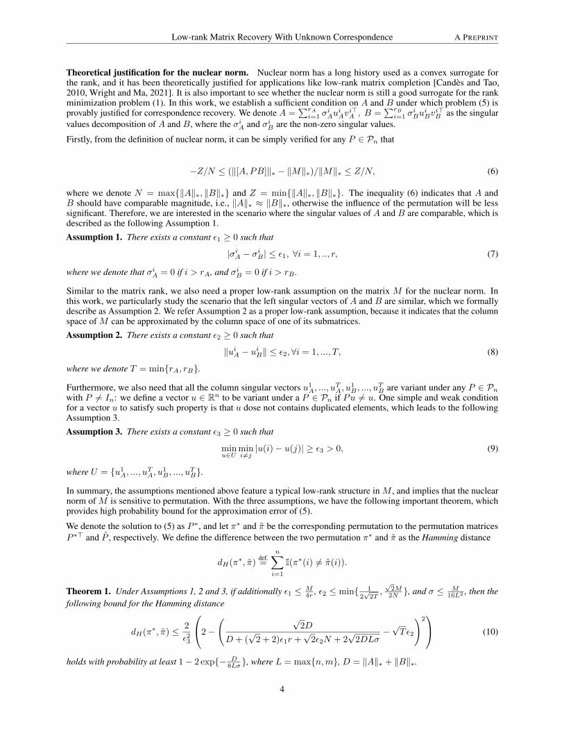
Theorem 1. Under Assumptions 1, 2 and 3, if additionally ε1 ≤ M4r , ε2 ≤ min 1

2√

2T,√

2M2N , and σ ≤ M

16L2 , then thefollowing bound for the Hamming distance

dH(π∗, π) ≤ 2

ε23

2−

( √2D

D + (√

2 + 2)ε1r +√

2ε2N + 2√

2DLσ−√Tε2

)2 (10)

holds with probability at least 1− 2 exp− D8Lσ, where L = maxn,m, D = ‖A‖∗ + ‖B‖∗.

4

Low-rank Matrix Recovery With Unknown Correspondence A PREPRINT

The proof to all the aforementioned theoretical results are provided in Appendix A.1.

Remark 1. From Theorem 1 we can see that when ε3 > 0, and ε1 → 0, ε2 → 0, σ → 0, the error dH(π∗, π) willconverge to zero with probability 1. Furthermore, we can also discover that the correspondence can be difficult torecover when:

• The rank of original matrix M is high, which can be seen from (10).• The magnitude of A and B w.r.t rank or nuclear norm are not comparable, which can be seen from (6) and (7).• The strength of noise is high, which can be seen from (10) and the probability in Theorem 1.

Notably, the numerical experiments in Section 4.1 corroborate our claims as well.

Figure 1: The relationship (11) under different percentages of observable entries.

Remark 2. Additionally, from the proof of Theorem 1 we find that the fundamental reason for the success of (5) is thatif M satisfies the previous assumptions, we have

‖[A,PB]‖∗/‖M‖∗ ≈ O(

(1−H(πP )/2n)− 1

2

). (11)

In many applications, we can only observe part of the full data. Therefore, it is also worthwhile to investigate whether(11) still holds when we can only access a small subset of the entries in Mo. Notably, Figure 1 gives the positive answerand shows that the relationship (11) is gracefully degraded when the percentage of observable entries is decreasing.This phenomenon is remarkable since it indicates the original correspondence can be recovered from only part of thefull data. The matrices used to generate Figure 1 are the same as those in Section 4.1, and the nuclear norm is computedapproximately by first filling the missing entries using Soft-Impute algorithm [Mazumder et al., 2010].

3 Algorithm

In this section, we consider the scenario with missing values, i.e., our observed data is PΩ(Mo) = PΩ([Ao, Bo]), wherePΩ is an operator that selects entries that are in the set of observable indices Ω. In this scenario, problem (5) can not bedirectly used since the evaluation of the nuclear norm and optimization of the permutation are coupled together. Inspiredby the matrix completion method [Hastie et al., 2015, Mazumder et al., 2010], we propose to solve an alternative formof (5) as follows,

minM∈Rn×m

minP∈Pn

∥∥∥PΩ([Ao, PBo])− PΩ(M)∥∥∥2

F+ λ

∥∥∥M∥∥∥∗, (12)

where λ > 0 is the penalty coefficient. We denote that M = [MA, MB ] and MA, MB are the two submatrices with thesame dimension as Ao and Bo respectively. We can write (12) equivalently as

minM∈Rn×m

minP∈Pn

∥∥∥PΩ(Ao)− PΩ(MA)∥∥∥2

F+ 〈C(MB), P 〉+ λ

∥∥∥M∥∥∥∗, (13)

5

Low-rank Matrix Recovery With Unknown Correspondence A PREPRINT

where C(MB) ∈ Rn×n is the pairing cost matrix with

C(MB)(i, j) =∑

(j,j′′)∈Ω

(MB(i, j′′)−Bo(j, j′′)

)2

, ∀i, j = 1, ..., n.

Baseline algorithm. A conventional strategy to handle an optimization problem like (13) is the alternating minimizationor the block coordinate descent algorithm [Abid et al., 2017]. Specifically, it executes the following two updatesiteratively until converge.

M new ← arg minM∈Rn×m

∥∥∥PΩ([Ao, PoldBo])− PΩ(M)

∥∥∥2

F+ λ

∥∥∥M∥∥∥∗, (14)

P new ← arg minP∈Pn

〈C(M newB ), P 〉. (15)

The first update step (14) is a convex optimization problem and can be solved by the proximal gradient algorithm[Mazumder et al., 2010]. The second update step (15) is actually a discrete optimal transport problem which can besolved by the classical Hungarian algorithm with time complexity O(n3) [Jonker and Volgenant, 1986]. However, aswe will see in the Section 4, this algorithm performs poorly, and it is likely to fall into an undesirable local solutionquickly in practice. Specifically, the main reason is that the solution of (15) is often not unique and a small change inMB would lead to large change of P . To address this issue, we propose a novel and efficient algorithm M3O algorithmbased on the entropic optimal transport [Peyré et al., 2019] and min-max optimization [Jin et al., 2020a].

Smoothing the permutation with entropy regularization. For any a ∈ Rn, b ∈ Rm, we define

Π(a, b) = S ∈ Rn×m : S1m = a, S>1n = b, S(i, j) ≥ 0, ∀i, j,

which is also known as the Birkhoff polytope. The famous Birkhoff-von Neumann theorem [Birkhoff, 1946] states thatthe set of extremal points of Π(1n,1n) is equal to Pn. Inspired by [Xie et al., 2021] and the interior point method forlinear programming [Bertsekas, 1997], in order to smooth the optimization process of the baseline algorithm, we relaxP from being an exact permutation matrix, i.e., to keep P staying inside the Birkhoff polytope Π(1n,1n). That is, wepropose to replace the combinatorial problem (15) with the following continuous optimization problem

minP∈Π(1n,1n)

〈C(MB), P 〉+ εH(P ), (16)

whereH(P )def.=∑i,j P (i, j)(log(P (i, j))−1) is the matrix negative entropy and ε > 0 is the regularization coefficient.

Notably, (16) is also known as the Entropic Optimal Transport (EOT) problem [Peyré et al., 2019], which is a stronglyconvex optimization problem and can be solved roughly in theO(n2) complexity by the Sinkhorn algorithm. Specifically,the Sinkhorn algorithm solves the dual problem of (16),

maxα,β∈Rn

Wε(MB , α, β)def.= 〈1n, α〉+ 〈1n, β〉 − ε

⟨1n×n, exp

α⊕ β − C(MB)

ε

⟩, (17)

which reduces the variables dimension from n2 to 2n and is thus greatly favorable in the high dimension scenario. Bysubstituting the inner minimization problem of (13) with (16), we end up with solving the following unconstrainedmin-max optimization problem

minM

maxα,β

∥∥∥A− MA

∥∥∥2

F+Wε(MB , α, β) + λ

∥∥∥M∥∥∥∗. (18)

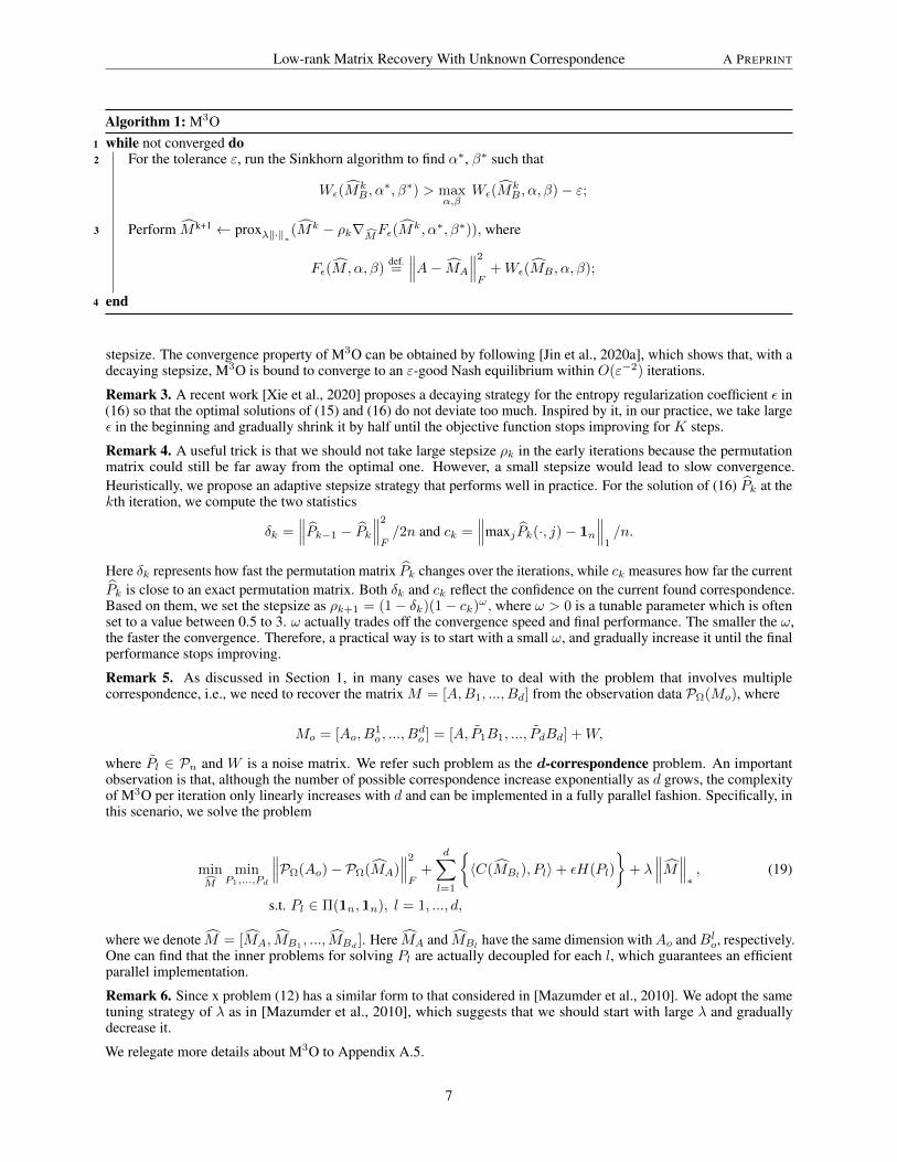
Follows the idea of [Jin et al., 2020a], we consider to adopt a proximal gradient algorithm with a Max-Oracle for(18). Specifically, we employ the Skinhorn algorithm [Peyré et al., 2019] as the Max-Oracle to retrieve an ε-goodsolution of the inner max problem (17). We summarize our proposed algorithm M3O (Matrix recovery via Min-MaxOptimization) in Algorithm 1, where proxλ‖·‖∗(·) is the proximal operator of nuclear norm and ρk is the gradient

6

Low-rank Matrix Recovery With Unknown Correspondence A PREPRINT

Algorithm 1: M3O1 while not converged do2 For the tolerance ε, run the Sinkhorn algorithm to find α∗, β∗ such that

Wε(MkB , α

∗, β∗) > maxα,β

Wε(MkB , α, β)− ε;

3 Perform M k+1 ← proxλ‖·‖∗(Mk − ρk∇MFε(M

k, α∗, β∗)), where

Fε(M, α, β)def.=∥∥∥A− MA

∥∥∥2

F+Wε(MB , α, β);

4 end

stepsize. The convergence property of M3O can be obtained by following [Jin et al., 2020a], which shows that, with adecaying stepsize, M3O is bound to converge to an ε-good Nash equilibrium within O(ε−2) iterations.

Remark 3. A recent work [Xie et al., 2020] proposes a decaying strategy for the entropy regularization coefficient ε in(16) so that the optimal solutions of (15) and (16) do not deviate too much. Inspired by it, in our practice, we take largeε in the beginning and gradually shrink it by half until the objective function stops improving for K steps.

Remark 4. A useful trick is that we should not take large stepsize ρk in the early iterations because the permutationmatrix could still be far away from the optimal one. However, a small stepsize would lead to slow convergence.Heuristically, we propose an adaptive stepsize strategy that performs well in practice. For the solution of (16) Pk at thekth iteration, we compute the two statistics

δk =∥∥∥Pk−1 − Pk

∥∥∥2

F/2n and ck =

∥∥∥maxjPk(·, j)− 1n

∥∥∥1/n.

Here δk represents how fast the permutation matrix Pk changes over the iterations, while ck measures how far the currentPk is close to an exact permutation matrix. Both δk and ck reflect the confidence on the current found correspondence.Based on them, we set the stepsize as ρk+1 = (1− δk)(1− ck)ω, where ω > 0 is a tunable parameter which is oftenset to a value between 0.5 to 3. ω actually trades off the convergence speed and final performance. The smaller the ω,the faster the convergence. Therefore, a practical way is to start with a small ω, and gradually increase it until the finalperformance stops improving.

Remark 5. As discussed in Section 1, in many cases we have to deal with the problem that involves multiplecorrespondence, i.e., we need to recover the matrix M = [A,B1, ..., Bd] from the observation data PΩ(Mo), where

Mo = [Ao, B1o , ..., B

do ] = [A, P1B1, ..., PdBd] +W,

where Pl ∈ Pn and W is a noise matrix. We refer such problem as the d-correspondence problem. An importantobservation is that, although the number of possible correspondence increase exponentially as d grows, the complexityof M3O per iteration only linearly increases with d and can be implemented in a fully parallel fashion. Specifically, inthis scenario, we solve the problem

minM

minP1,...,Pd

∥∥∥PΩ(Ao)− PΩ(MA)∥∥∥2

F+

d∑l=1

〈C(MBl

), Pl〉+ εH(Pl)

+ λ

∥∥∥M∥∥∥∗, (19)

s.t. Pl ∈ Π(1n,1n), l = 1, ..., d,

where we denote M = [MA, MB1 , ..., MBd]. Here MA and MBl

have the same dimension withAo andBlo, respectively.One can find that the inner problems for solving Pl are actually decoupled for each l, which guarantees an efficientparallel implementation.

Remark 6. Since x problem (12) has a similar form to that considered in [Mazumder et al., 2010]. We adopt the sametuning strategy of λ as in [Mazumder et al., 2010], which suggests that we should start with large λ and graduallydecrease it.

We relegate more details about M3O to Appendix A.5.

7

Low-rank Matrix Recovery With Unknown Correspondence A PREPRINT

(a) Objective value (b) Permutation error

Figure 2: Performance of various algorithms on a simulated 1-correspondence problem.

4 Experiments

In this section, we evaluate our proposed M3O on both synthetic and real-world datasets, including the MovieLens 100Kand the Extended Yale B dataset. We also provide an ablation study for the decaying entropy regularization strategyand the adaptive stepsize strategy proposed in Remarks 3 and 4. In all the experiments, we employ the Soft-Imputealgorithm [Mazumder et al., 2010] as a standard algorithm for matrix completion. Extra experiment details and auxiliaryresults can be found in Appendix A.8.

Algorithms. We denote the following algorithms for comparison in all the experiments:

1. Oracle: Running the Soft-Impute algorithm with ground-truth correspondence.2. Baseline: The Baseline algorithm in (14) and (15).3. MUS: Since there is currently no existing algorithm directly applicable to the scenario considered by (19), inspired

by [Yao et al., 2021], we modify and extend the algorithm in [Zhang and Li, 2020], which is originally proposedfor the MUS problem, to deal with the MRUC problem. The details of the adapted algorithm are provided inAppendix A.7.

4.1 Synthetic data

We first investigate the property of our proposed M3O algorithm on the synthetic data.

Data generation. We generate the original data matrix in this form M = RE + ηW, where R ∈ Rn×r, E ∈Rr×m, W ∈ Rn×m and η > 0 indicates the strength of the additive noise. The entries of R, E, W are all i.i.dsampled from the N (0, 1). Then we split the data matrix M by M = [A,B1, ..., Bd] where we denote A ∈ Rn×mA ,B1 ∈ Rn×m1 , ..., Bd ∈ Rn×md to represent data from d + 1 data sources. The permuted observation matrix Mo

is obtained by first generating d permutation matrices P1, ..., Pd randomly and independently, and then computingMo = [A,P1B1, ..., PdBd]. Finally, we remove (1− |Ω| · 100%/(n ·m)) percent of the entries of Mo randomly anduniformly, where |Ω| indicating the number of observable entries.

Ablation study. We denote the following variants of M3O for the ablation study.

1. M3O-AS-DE: M3O with both Adpative Stepsize and Decaying Entropy regularization.2. M3O-DE: M3O with Decaying Entropy regularization only. M3O-DE-1 and M3O-DE-2 adopt constant stepsizeρk = 0.5 and ρk = 0.01, respectively.

3. M3O-AS: M3O with Adpative Stepsize only. The entropy coefficient ε is fixed to 0.0005.

In the following results, we denote πl as the corresponding permutation to Pl. We initialize M from Gaussiandistribution for the M3O algorithm and its variants. We choose initial ε as 0.1 and K = 100 as the default for thedecaying entropy regularization, and set ω = 3 as the default for the adaptive stepsize. We also report the achievedobjective values of (19) for the tested algorithms, except for the MUS algorithm since it has a different objective. Wedenote π as the recovered permutation.

Results. Figure 2 displays the result under the setting η = 0.1, |Ω| · 100%/(n ·m) = 80%, n = m = 100, r = 5,d = 1, mA = 60 and m1 = 40. The algorithm M3O-AS-DE achieves the best result, and can recover the ground-truthcorrespondence. M3O-AS behaves similarly to Baseline and MUS. They all converge to a poor local solution quickly.

8

Low-rank Matrix Recovery With Unknown Correspondence A PREPRINT

M3O-DE-1 converges quickly and also falls into a poor local solution due to large stepsize, while M3O-DE-2 adopts asmall stepsize and hence suffers from slow convergence. Due to the superiority of M3O-AS-DE over the other variants,in the following results, we refer M3O as M3O-AS-DE for short.

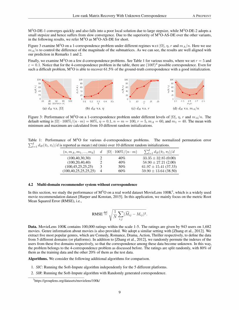
Figure 3 examine M3O on a 1-correspondence problem under different regimes w.r.t |Ω|, η, r and mA/n. Here we usemA/n to control the difference of the magnitude of the submatrices. As we can see, the results are well aligned withour prediction in Remarks 1 and 2.

Finally, we examine M3O on a few d-correspondence problems. See Table 1 for various results, where we set r = 5 andε = 0.1. Notice that for the 4-correspondence problem in the table, there are (100!)4 possible correspondence. Even forsuch a difficult problem, M3O is able to recover 61.5% of the ground-truth correspondence with a good initialization.

(a) dH v.s. |Ω| (b) dH v.s. η (c) dH v.s. r (d) dH v.s. mA/n

Figure 3: Performance of M3O on a 1-correspondence problem under different levels of |Ω|, η, r and mA/n. Thedefault setting is |Ω| · 100%/(n ·m) = 80%, η = 0.1, n = m = 100, r = 5, mA = 60, and m1 = 40. The mean withminimum and maximum are calculated from 10 different random initializations.

Table 1: Performance of M3O for various d-correspondence problems. The normalized permutation error∑dl=1 dH(πl, πl)/d is reported as mean±std (min) over 10 different random initializations.

(n,mA,m1, ...,md) d |Ω| · 100%/(n ·m)∑dl=1 dH(πl, πl)/d

(100,40,30,30) 2 40% 33.35± 32.85 (0.00)(100,20,40,40) 2 40% 58.90± 27.21 (2.00)

(100,45,25,25,25) 3 50% 61.97± 15.41 (37.33)(100,40,25,25,25,25) 4 60% 59.90± 13.64 (38.50)

4.2 Multi-domain recommender system without correspondence

In this section, we study the performance of M3O on a real world dataset MovieLens 100K3, which is a widely usedmovie recommendation dataset [Harper and Konstan, 2015]. In this application, we mainly focus on the metric RootMean Squared Error (RMSE), i.e.,

RMSE def.=

√1

N

∑i,j

(Mij −Mij)2.

Data. MovieLens 100K contains 100,000 ratings within the scale 1-5. The ratings are given by 943 users on 1,682movies. Genre information about movies is also provided. We adopt a similar setting with [Zhang et al., 2012]. Weextract five most popular genres, which are Comedy, Romance, Drama, Action, Thriller respectively, to define the datafrom 5 different domains (or platforms). In addition to [Zhang et al., 2012], we randomly permute the indexes of theusers from these five domains respectively, so that the correspondence among these data become unknown. In this way,the problem belongs to the 4-correspondence problem as discussed before. The ratings are split randomly, with 80% ofthem as the training data and the other 20% of them as the test data.

Algorithms. We consider the following additional algorithms for comparison.

1. SIC: Running the Soft-Impute algorithm independently for the 5 different platforms.

2. SIR: Running the Soft-Impute algorithm with Randomly generated correspondence.

3https://grouplens.org/datasets/movielens/100k/

9

Low-rank Matrix Recovery With Unknown Correspondence A PREPRINT

Results. As discussed in experiments on the simulated data, the exact recovery of correspondence becomes impossibledue to the small amount of observable entries. Therefore, in the following experiment, since exact correspondenceis not needed, we fix ε = 0.05 for M3O. Table 2 shows the results by averaging the RMSE on the test data over 10different random seeds.

We can first see that the matrix completion with a wrong correspondence, i.e., SIR, can be harmful to the overallperformance since it is even worse than the results of SIC. Notably, although the ground-truth correspondence can notbe recovered, each platform can still benefit from M3O since it improves the performance over SIC. This is mainlybecause M3O is still able to correspond similar users for inferring missing ratings. On the contrary, since both Baselineand MUS can only establish an exact one-to-one correspondence for each user, they fail to improve SIC significantly.Remarkably, M3O is only inferior to the Oracle method a little, and even achieves lower test RMSE than the Oraclemethod on the Comedy genre.

Table 2: Test RMSE of various algorithms on MovieLens 100KMethod Comedy Romance Drama Action Thriller Total

SIR 1.0202 1.0158 0.9808 0.9803 0.9811 0.9944SIC 0.9694 0.9695 0.9317 0.9175 0.9253 0.9418

MUS 0.9659 0.9842 0.9423 0.9305 0.9306 0.9485Baseline 0.9728 0.9562 0.9379 0.9105 0.9145 0.9395

M3O 0.9389 0.8787 0.9139 0.8556 0.8567 0.8948Oracle 0.9444 0.7825 0.9058 0.8176 0.8098 0.8667

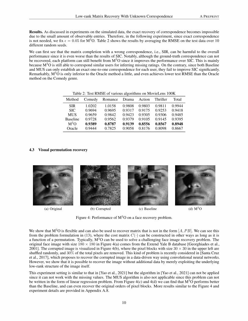
4.3 Visual permutation recovery

(a) Original (b) Corrupted (c) Baseline (d) M3O

Figure 4: Performance of M3O on a face recovery problem.

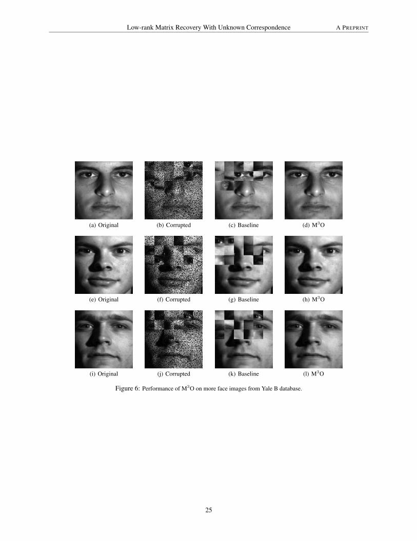
We show that M3O is flexible and can also be used to recover matrix that is not in the form [A,PB]. We can see thisfrom the problem formulation in (13), where the cost matrix C(·) can be constructed in other ways as long as it isa function of a permutation. Typically, M3O can be used to solve a challenging face image recovery problem. Theoriginal face image with size 180 × 180 in Figure 4(a) comes from the Extend Yale B database [Georghiades et al.,2001]. The corrupted image is visualized in Figure 4(b), where the pixel blocks with size 30× 30 in the upper left areshuffled randomly, and 30% of the total pixels are removed. This kind of problem is recently considered in [Santa Cruzet al., 2017], which proposes to recover the corrupted image in a data-driven way using convolutional neural networks.However, we show that it is possible to recover the image without additional data by merely exploiting the underlyinglow-rank structure of the image itself.

This experiment setting is similar to that in [Yao et al., 2021] but the algorithm in [Yao et al., 2021] can not be appliedsince it can not work with the missing values. The MUS algorithm is also not applicable since this problem can notbe written in the form of linear regression problem. From Figure 4(c) and 4(d) we can find that M3O performs betterthan the Baseline, and can even recover the original orders of pixel blocks. More results similar to the Figure 4 andexperiment details are provided in Appendix A.8.

10

Low-rank Matrix Recovery With Unknown Correspondence A PREPRINT

5 Conclusion

In this paper, we have studied the important MRUC problem where part of the observed submatrix is shuffled. Thisproblem has not been well explored in the existing literature. Theoretically, we are the first to rigorously analyze the roleof low-rank model in the MRUC problem, and is also the first to show that minimizing nuclear norm is provably efficientfor recovering a typical low-rank matrix. For practical implementations, we propose a highly efficient algorithm, theM3O algorithm, which is shown to consistently achieve the best performance over several baselines in all the testedscenarios.

It is worthwhile to point out that apart from the two applications we have studied in this paper, this problem couldarise in more scenarios like the gnome assembly problem [Huang and Madan, 1999], the video pose tracking problem[Ganapathi et al., 2012] and the privacy-aware sensor networks [Gruteser et al., 2003], etc. We believes that our workprovides a general framework to deal with unknown correspondence issue in these scenarios.

As we have shown in Figure 3, one major limit of our algorithm is the sensitivity to the initialization. The phenomenonis exacerbated when the additive noise is high or the numbers of observable entries are small. We suggest to try with afew different initialization strategy when applying M3O to a specific task. Finding stable initialization strategy is alsoan important task for our future works.

ReferencesJayakrishnan Unnikrishnan, Saeid Haghighatshoar, and Martin Vetterli. Unlabeled sensing with random linear

measurements. IEEE Transactions on Information Theory, 64(5):3237–3253, 2018.

Marco Gruteser, Graham Schelle, Ashish Jain, Richard Han, and Dirk Grunwald. Privacy-aware location sensornetworks. In HotOS, volume 3, pages 163–168, 2003.

Debasmit Das and C. S. George Lee. Sample-to-Sample Correspondence for Unsupervised Domain Adap-tation. Engineering Applications of Artificial Intelligence, 73:80–91, August 2018. ISSN 09521976.doi:10.1016/j.engappai.2018.05.001. URL http://arxiv.org/abs/1805.00355. arXiv: 1805.00355.

Pan Ji, Hongdong Li, Mathieu Salzmann, and Yuchao Dai. Robust motion segmentation with unknown correspondence.In European conference on computer vision, pages 204–219. Springer, 2014.

Zinan Zeng, Tsung-Han Chan, Kui Jia, and Dong Xu. Finding correspondence from multiple images via sparse andlow-rank decomposition. In European Conference on Computer Vision, pages 325–339. Springer, 2012.

Xiaowei Zhou, Menglong Zhu, and Kostas Daniilidis. Multi-image matching via fast alternating minimization. InProceedings of the IEEE International Conference on Computer Vision, pages 4032–4040, 2015.

Hock-Peng Chan and Wei-Liem Loh. A file linkage problem of degroot and goel revisited. Statistica Sinica, pages1031–1045, 2001.

Liu Yang, Ben Tan, Vincent W Zheng, Kai Chen, and Qiang Yang. Federated recommendation systems. In FederatedLearning, pages 225–239. Springer, 2020.

John Wright and Yi Ma. High-Dimensional Data Analysis with Low-Dimensional Models: Principles, Computation,and Applications. Cambridge University Press, 2021.

Rahul Mazumder, Trevor Hastie, and Robert Tibshirani. Spectral regularization algorithms for learning large incompletematrices. The Journal of Machine Learning Research, 11:2287–2322, 2010. Publisher: JMLR. org.

Trevor Hastie, Rahul Mazumder, Jason D. Lee, and Reza Zadeh. Matrix completion and low-rank SVD via fastalternating least squares. The Journal of Machine Learning Research, 16(1):3367–3402, 2015. Publisher: JMLR.org.

J Ben Schafer, Dan Frankowski, Jon Herlocker, and Shilad Sen. Collaborative filtering recommender systems. In Theadaptive web, pages 291–324. Springer, 2007.

Yu Zhang, Bin Cao, and Dit-Yan Yeung. Multi-domain collaborative filtering. arXiv preprint arXiv:1203.3535, 2012.

Rodrigo Santa Cruz, Basura Fernando, Anoop Cherian, and Stephen Gould. Deeppermnet: Visual permutation learning.In Proceedings of the IEEE Conference on Computer Vision and Pattern Recognition, pages 3949–3957, 2017.

Ashwin Pananjady, Martin J Wainwright, and Thomas A Courtade. Denoising linear models with permuted data. In2017 IEEE International Symposium on Information Theory (ISIT), pages 446–450. IEEE, 2017a.

Hang Zhang, Martin Slawski, and Ping Li. The benefits of diversity: Permutation recovery in unlabeled sensing frommultiple measurement vectors. arXiv preprint arXiv:1909.02496, 2019a.

11

Low-rank Matrix Recovery With Unknown Correspondence A PREPRINT

Hang Zhang, Martin Slawski, and Ping Li. Permutation recovery from multiple measurement vectors in unlabeledsensing. In 2019 IEEE International Symposium on Information Theory (ISIT), pages 1857–1861. IEEE, 2019b.

Hang Zhang and Ping Li. Optimal estimator for unlabeled linear regression. In International Conference on MachineLearning, pages 11153–11162. PMLR, 2020.

Martin Slawski, Mostafa Rahmani, and Ping Li. A sparse representation-based approach to linear regression withpartially shuffled labels. In Uncertainty in Artificial Intelligence, pages 38–48. PMLR, 2020a.

Martin Slawski, Emanuel Ben-David, and Ping Li. Two-stage approach to multivariate linear regression with sparselymismatched data. J. Mach. Learn. Res., 21(204):1–42, 2020b.

Yunzhen Yao, Liangzu Peng, and Manolis C Tsakiris. Unlabeled principal component analysis. arXiv preprintarXiv:2101.09446, 2021.

David S Dummit and Richard M Foote. Abstract algebra, volume 1999. Prentice Hall Englewood Cliffs, NJ, 1991.

Emmanuel J Candès and Terence Tao. The power of convex relaxation: Near-optimal matrix completion. IEEETransactions on Information Theory, 56(5):2053–2080, 2010.

Abubakar Abid, Ada Poon, and James Zou. Linear regression with shuffled labels. arXiv preprint arXiv:1705.01342,2017.

Roy Jonker and Ton Volgenant. Improving the hungarian assignment algorithm. Operations Research Letters, 5(4):171–175, 1986.

Gabriel Peyré, Marco Cuturi, et al. Computational optimal transport: With applications to data science. Foundationsand Trends® in Machine Learning, 11(5-6):355–607, 2019.

Chi Jin, Praneeth Netrapalli, and Michael Jordan. What is local optimality in nonconvex-nonconcave minimaxoptimization? In International Conference on Machine Learning, pages 4880–4889. PMLR, 2020a.

Garrett Birkhoff. Three observations on linear algebra. Univ. Nac. Tacuman, Rev. Ser. A, 5:147–151, 1946.

Yujia Xie, Yixiu Mao, Simiao Zuo, Hongteng Xu, Xiaojing Ye, Tuo Zhao, and Hongyuan Zha. A hypergradientapproach to robust regression without correspondence. In International Conference on Learning Representations,2021. URL https://openreview.net/forum?id=l35SB-_raSQ.

Dimitri P Bertsekas. Nonlinear programming. Journal of the Operational Research Society, 48(3):334–334, 1997.

Yujia Xie, Xiangfeng Wang, Ruijia Wang, and Hongyuan Zha. A fast proximal point method for computing exactwasserstein distance. In Ryan P. Adams and Vibhav Gogate, editors, Proceedings of The 35th Uncertainty in ArtificialIntelligence Conference, volume 115 of Proceedings of Machine Learning Research, pages 433–453. PMLR, 22–25Jul 2020. URL https://proceedings.mlr.press/v115/xie20b.html.

F Maxwell Harper and Joseph A Konstan. The movielens datasets: History and context. Acm transactions on interactiveintelligent systems (tiis), 5(4):1–19, 2015.

A.S. Georghiades, P.N. Belhumeur, and D.J. Kriegman. From few to many: Illumination cone models for facerecognition under variable lighting and pose. IEEE Trans. Pattern Anal. Mach. Intelligence, 23(6):643–660, 2001.

Xiaoqiu Huang and Anup Madan. Cap3: A dna sequence assembly program. Genome research, 9(9):868–877, 1999.

Varun Ganapathi, Christian Plagemann, Daphne Koller, and Sebastian Thrun. Real-time human pose tracking fromrange data. In European conference on computer vision, pages 738–751. Springer, 2012.

Bumsub Ham, Minsu Cho, Cordelia Schmid, and Jean Ponce. Proposal flow: Semantic correspondence from objectproposals. IEEE transactions on pattern analysis and machine intelligence, 40(7):1711–1725, 2017. Publisher:IEEE.

Kui Jia, Tsung-Han Chan, Zinan Zeng, Shenghua Gao, Gang Wang, Tianzhu Zhang, and Yi Ma. ROML: A robustfeature correspondence approach for matching objects in a set of images. International Journal of Computer Vision,117(2):173–197, 2016. Publisher: Springer.

Xiaolong Wang, Allan Jabri, and Alexei A. Efros. Learning correspondence from the cycle-consistency of time. InProceedings of the IEEE/CVF Conference on Computer Vision and Pattern Recognition, pages 2566–2576, 2019.

Tinghui Zhou, Philipp Krahenbuhl, Mathieu Aubry, Qixing Huang, and Alexei A. Efros. Learning dense correspondencevia 3d-guided cycle consistency. In Proceedings of the IEEE Conference on Computer Vision and Pattern Recognition,pages 117–126, 2016.

Amin Nejatbakhsh and Erdem Varol. Robust approximate linear regression without correspondence. arXiv preprintarXiv:1906.00273, 2019.

12

Low-rank Matrix Recovery With Unknown Correspondence A PREPRINT

Babak Barazandeh and Meisam Razaviyayn. Solving Non-Convex Non-Differentiable Min-Max Games Using ProximalGradient Method. In ICASSP 2020-2020 IEEE International Conference on Acoustics, Speech and Signal Processing(ICASSP), pages 3162–3166. IEEE, 2020.

Jiawei Zhang, Peijun Xiao, Ruoyu Sun, and Zhi-Quan Luo. A Single-Loop Smoothed Gradient Descent-AscentAlgorithm for Nonconvex-Concave Min-Max Problems. arXiv preprint arXiv:2010.15768, 2020.

Tianyi Lin, Chi Jin, and Michael Jordan. On gradient descent ascent for nonconvex-concave minimax problems. InInternational Conference on Machine Learning, pages 6083–6093. PMLR, 2020.

Chi Jin, Praneeth Netrapalli, and Michael Jordan. What is local optimality in nonconvex-nonconcave minimaxoptimization? In International Conference on Machine Learning, pages 4880–4889. PMLR, 2020b.

Kiran K. Thekumparampil, Prateek Jain, Praneeth Netrapalli, and Sewoong Oh. Efficient algorithms for smoothminimax optimization. In Advances in Neural Information Processing Systems, pages 12680–12691, 2019.

Paul Tseng. On accelerated proximal gradient methods for convex-concave optimization. submitted to SIAM Journalon Optimization, 2(3), 2008.

Constantinos Daskalakis and Ioannis Panageas. The limit points of (optimistic) gradient descent in min-max optimization.In Advances in Neural Information Processing Systems, pages 9236–9246, 2018.

Hassan Rafique, Mingrui Liu, Qihang Lin, and Tianbao Yang. Non-convex min-max optimization: Provable algorithmsand applications in machine learning. arXiv preprint arXiv:1810.02060, 2018.

Yurii Nesterov. Dual extrapolation and its applications to solving variational inequalities and related problems.Mathematical Programming, 109(2-3):319–344, 2007. Publisher: Springer.

Anatoli Juditsky and Arkadi Nemirovski. Solving variational inequalities with monotone operators on domains givenby linear minimization oracles. Mathematical Programming, 156(1-2):221–256, 2016. Publisher: Springer.

Sijia Liu, Songtao Lu, Xiangyi Chen, Yao Feng, Kaidi Xu, Abdullah Al-Dujaili, Mingyi Hong, and Una-May O’Reilly.Min-max optimization without gradients: Convergence and applications to black-box evasion and poisoning attacks.In International Conference on Machine Learning, pages 6282–6293. PMLR, 2020.

Arkadi Nemirovski. Prox-method with rate of convergence O (1/t) for variational inequalities with Lipschitz continuousmonotone operators and smooth convex-concave saddle point problems. SIAM Journal on Optimization, 15(1):229–251, 2004. Publisher: SIAM.

Maher Nouiehed, Maziar Sanjabi, Tianjian Huang, Jason D. Lee, and Meisam Razaviyayn. Solving a class of non-convex min-max games using iterative first order methods. In Advances in Neural Information Processing Systems,pages 14934–14942, 2019.

Meisam Razaviyayn, Tianjian Huang, Songtao Lu, Maher Nouiehed, Maziar Sanjabi, and Mingyi Hong. Nonconvexmin-max optimization: Applications, challenges, and recent theoretical advances. IEEE Signal Processing Magazine,37(5):55–66, 2020. Publisher: IEEE.

Songtao Lu, Ioannis Tsaknakis, Mingyi Hong, and Yongxin Chen. Hybrid block successive approximation for one-sidednon-convex min-max problems: algorithms and applications. IEEE Transactions on Signal Processing, 2020.Publisher: IEEE.

Kim-Chuan Toh and Sangwoon Yun. An accelerated proximal gradient algorithm for nuclear norm regularized linearleast squares problems. Pacific Journal of optimization, 6(615-640):15, 2010.

Daniel Billsus, Michael J Pazzani, et al. Learning collaborative information filters. In Icml, volume 98, pages 46–54,1998.

Frederik Schaffalitzky and Andrew Zisserman. Multi-view matching for unordered image sets, or “how do i organizemy holiday snaps?”. In European conference on computer vision, pages 414–431. Springer, 2002.

Dimitris Bertsimas and John N Tsitsiklis. Introduction to linear optimization, volume 6. Athena Scientific Belmont,MA, 1997.

Sanjay Mehrotra. On the implementation of a primal-dual interior point method. SIAM Journal on optimization, 2(4):575–601, 1992.

Michael Grant and Stephen Boyd. Cvx: Matlab software for disciplined convex programming, version 2.1, 2014.

Yu Zheng. Methodologies for cross-domain data fusion: An overview. IEEE transactions on big data, 1(1):16–34,2015.

Qiang Yang, Yang Liu, Tianjian Chen, and Yongxin Tong. Federated machine learning: Concept and applications. ACMTransactions on Intelligent Systems and Technology (TIST), 10(2):1–19, 2019.

13

Low-rank Matrix Recovery With Unknown Correspondence A PREPRINT

Ashwin Pananjady, Martin J Wainwright, and Thomas A Courtade. Linear regression with shuffled data: Statistical andcomputational limits of permutation recovery. IEEE Transactions on Information Theory, 64(5):3286–3300, 2017b.

Zhidong Bai and Tailen Hsing. The broken sample problem. Probability theory and related fields, 131(4):528–552,2005.

Daniel Hsu, Kevin Shi, and Xiaorui Sun. Linear regression without correspondence. arXiv preprint arXiv:1705.07048,2017.

Morris H DeGroot and Prem K Goel. Estimation of the correlation coefficient from a broken random sample. TheAnnals of Statistics, pages 264–278, 1980.

Joseph B Kruskal. Three-way arrays: rank and uniqueness of trilinear decompositions, with application to arithmeticcomplexity and statistics. Linear algebra and its applications, 18(2):95–138, 1977.

Paul R Halmos. Measure theory, volume 18. Springer, 2013.Martin J Wainwright. High-dimensional statistics: A non-asymptotic viewpoint, volume 48. Cambridge University

Press, 2019.

A Appendix

A.1 Proof for the Theoretical Results

Proof of Proposition 1. We denote that a1, .., arA as the linear bases of the column space of A. We can extend them tothe bases of the column space of M as a1, .., arA , b1, ..., br−rA . In this way, there must exists a matrix Q ∈ Rr×mB

such thatB = [a1, .., arA , b1, ..., br−rA ]Q.

Hence, we havePB = [Pa1, .., ParA , P b1, ..., P br−rA ]Q.

Similarly, there must exists a matrix T ∈ RrA×mA such thatA = [a1, .., arA ]T.

Hence, we obtain that

[A,PB] = [a1, .., arA , Pa1, .., ParA , P b1, ..., P br−rA ]

[T 00 Q

].

Now, we haverank([A,PB]) ≤ rank([a1, .., arA , Pa1, .., ParA , P b1, ..., P br−rA ])

≤ rank([a1, .., arA , Pa1, .., ParA ]) + r − rA

= rank([a1, .., arA , Pa1, .., ParA ]

[IrA −IrA0 IrA

]) + r − rA

≤ rA + r − rA + rank([Pa1 − a1, .., ParA − arA ]). (20)

Now we denote the cycles in πP with length greater than 1 as C1, ..., CC(πP ), and ζ1, ..., ζn−H(πp) as the indexes thatare not in any one of C1, ..., CC(πP ). We construct a matrix Y ∈ R(n+C(πP )−H(πp))×n as:

Y (i, j) = 1 if j = ζi else Y (i, j) = 0, for i = 1, ..., (n−H(πp));

Y (i, j) = 1 ∀j ∈ Ci, and Y (i, j) = 0 ∀j /∈ Ci,for i = (n−H(πp) + 1), ..., (n+ C(πP )−H(πp)).

It can be verified thatY (Pai − ai) = 0, i = 1, ..., rA.

We denote the null space of Y as Null(Y ) = x ∈ Rn|Y x = 0. From the construction of Y we can see thatdim(Null(Y )) = H(πP )− C(πP ). Hence we have

rank([Pa1 − a1, .., ParA − arA ]) ≤ H(πP )− C(πP ). (21)

On the other hand, we haverank([A,PB]) ≤ rank(A) + rank(PB) = rank(A) + rank(B) = rA + rB . (22)

Combining (20), (21) and (22) , we can obtain (3).

14

Low-rank Matrix Recovery With Unknown Correspondence A PREPRINT

Following the proof of Proposition 1, it is easy to show the similar result for the case with multiple permutation, whichis summarized as the Corollary 1Corollary 1. For the matrix M = [A,B1, .., Bd] ∈ Rn×m with rank(M) = r, rank(A) = rA, and rank(Bi) = rBi ,i = 1, ...d, we have ∀P1, ..., Pd ∈ Pn,

rank([A,P1B1, ..., PdBd]) ≤ minn,m, rA +

d∑i=1

rBi, r +

d∑i=1

H(πPi)− C(πPi

). (23)

Proof of Proposition 2. To prove Proposition 2, we need an important lemma on measure theory from [Halmos, 2013].

Lemma 1. Let p(x) be a polynomial on Rn. If there exists a x0 ∈ Rn such that p(x0) 6= 0, then the Lebesgue measureof the set x|p(x) = 0 is 0.

∀P ∈ Pn, we define the polynomial on Rn×r ⊗ Rr×m as

prP (R,E) =∑

S∈Sr([A,PB])

det(S)2,

where det(·) is the determinant of matrix, and Sr(X) is the set of all r × r sub-matrices in X . We denote thatrP = min2r, r +H(πP )− C(πP ). We can see that rank([A,PB]) ≥ rP if and if only prPP (R,E) > 0. Therefore,from Lemma 1 and Proposition 1 we can conclude that if there exists two matrices R0 ∈ Rn×r and E0 ∈ Rr×m suchthat prPP ([R0, E0]) > 0, then rank([A,PB]) = rP holds with probability 1. In this way, we only need to constructsuch R0 and E0 for every P ∈ Pn. For simplicity, we denote that k = H(πp) − C(πP ). We will discuss how toconstruct such R0 and E0 for the two cases 0 < k ≤ n− r and k ≥ n− r, respectively.

(1) If 0 < k ≤ n− r:

We construct the matrix Y ∈ R(n+C(πP )−H(πp))×n the same way with that in the proof of Proposition 1. Firstly, weshow that Null(Y ) =col(P − I).

col(P − I) ⊆Null(Y ): We can verify that Y (P − I) = 0.

Null(Y ) ⊆col(P − I): This is equivalent to prove that Null(P − I) ⊆col(Y ). Now we have Px = x, ∀x ∈Null(P − I).It can be verified that if Px = x, then we must have x(s) = x(q) if s and q belong to the same cycle Ci, where Ci isone of the cycles in C1, ..., CC(πP ). By the definition of Y , we can see that x ∈ col(Y ).

Now we know that rank(P − I) =dim(Null(Y )) = k. We denote the eigen vectors of P − I with non-zero eigenvalues as φ1, ..., φk, and the eigen vectors with zero eigen values as φk+1, ..., φn. Now we have (P − I)φi = λiφi fori = 1, ..., k and (P − I)φi = λiφi for i = k + 1, ..., n.

We construct the matrices R0 and E0 as

R0 = [φ1 + φk+1, φmin2,k + φk+2, ..., φminr,k + φk+r],

E0 = [Ir,0r×(mA−r), Ir,0r×(mB−r)].

Now we have

A = [φ1 + φk+1, φmin2,k + φk+2, ..., φminr,k + φk+r,0n×(mA−r)],

B = [φ1 + φk+1, φmin2,k + φk+2, ..., φminr,k + φk+r,0n×(mB−r)],

since [A,B] = R0E0. Therefore, we have

rank([A,PB]) = rank([φ1 + φk+1, ..., φminr,k + φk+r, λ1φ1, ..., λminr,kφminr,k])

= rank([φk+1, ..., φk+r, φ1, .., φminr,k])

= r + mink, r = min2r, r + k.

Now rank([A,PB]) = rP by this construction of R0 and E0. Hence prPP ([R0, E0]) > 0.

(2) If k > n− r:

We denote that the length of a cycle C as len(C), and denote the cycle with maximum length among the C1, ..., CC(πP )

as C∗. Now we have

len(C∗) ≥ H(πP )

C(πP )≥ n

n− k>n

r≥ 2r.

15

Low-rank Matrix Recovery With Unknown Correspondence A PREPRINT

To simplify the notations, we assume that the cycle C∗ permute the first j numbers, i.e.,

C∗ = (123...(j − 2)(j − 1)j),

where j > 2r. We define the vector u as u = [1, 2, 3, ..., j − 2, j − 1, j, 0, ..., 0]> ∈ Rn, and denote the correspondingpermutation matrix to C∗ as P∗ ∈ Pn. We construct the matrices R0 and E0 as

R0 =[u P 2

∗ u . . . P 2r−2∗ u

],

E0 = [Ir,0r×(mA−r), Ir,0r×(mB−r)].

Now we have

A = [u, P 2∗ u, . . . , P

2r−2∗ u,0n×(mA−r)],

B = [u, P 2∗ u, . . . , P

2r−2∗ u,0n×(mB−r)].

Therefore, we have

rank([A,PB]) = rank([u, P∗u, . . . , P2r−1∗ u]) = 2r,

because now [u, P∗u, . . . , P2r−1∗ u] is a circulant matrix. Now rank([A,PB]) = rP = 2r by this construction of R0

and E0. Hence prPP ([R0, E0]) > 0.

Proof of Theorem 1. To prove Theorem 1, we need to derive a series results. We first start with a very importantinequality w.r.t nuclear norm.

Proposition 3. Let P be a permutation matrix, then,

‖A‖∗ + ‖B‖∗ ≥ ‖[A,PB]‖∗ ≥‖A‖∗ + ‖B‖∗

‖[UAV >A , PUBV >B ]‖≥ ‖A‖∗ + ‖B‖∗√

2. (24)

Based on (24), the general idea is that under the Assumptions 1, 2 and 3, we will have ‖M‖∗ ≈ ‖A‖∗+‖B‖∗√2

and‖[UAV >A , PUBV >B ]‖ → 1 as H(πP ) increases.

Firstly, we show that under the Assumptions 1, 2, the nuclear norm of the original matrix M will reach the lower boundin (24) approximately, which is summarized as Lemma 2.

Lemma 2. Under the Assumptions 1, 2, we have

‖M‖∗ ≤ (‖A‖∗ + ‖B‖∗)/√

2 + (√

2 + 1)ε1r + ε2 max‖A‖∗, ‖B‖∗. (25)

Then, we show that under the Assumptions 2, 3, ‖[UAV >A , PUBV >B ]‖ → 1 as H(πP ) increases, which is summarizedas Lemma 3.

Lemma 3. Under the Assumptions 2, 3, we have

‖[UAV >A , PUBV >B ]‖ ≤√

2−H(πP )ε23/2 +√Tε2. (26)

Finally, we need a classical result on the tail bound for the operator norm of Gaussian matrix, whose proof can be foundin [Wainwright, 2019].

Lemma 4. Consider the random matrix W ∈ Rn×m whose elements follow N (0, σ2) i.i.d. For any δ > 0, we have

‖W‖ ≤√L(2 + δ)σ (27)

holds with probability greater than 1− 2 exp−Lδ2

2 , where L = maxn,m.

Based on Lemma 4, we have

‖W‖∗ ≤ L‖W‖ ≤√MLσ

holds with probability greater than 1− 2 exp− M8Lσ.

16

Low-rank Matrix Recovery With Unknown Correspondence A PREPRINT

From Proposition 3, Lemma 2 and Lemma 3 we can know that, for any P ∈ Pn with H(πP ) satisfies that

M√2− H(πp)ε3

2 +√Tε2

− ‖W‖∗ >M√

2+ (√

2 + 1)ε1r + ε2N + ‖W‖∗,

we must have

‖Ao, PBo‖ ≥ ‖A,PB‖ − ‖W‖∗

≥ M√2− H(πp)ε23

2 +√Tε2

− ‖W‖∗

>M√

2+ (√

2 + 1)ε1r + ε2N + ‖W‖∗

≥ ‖A,B‖∗ + ‖W‖∗ ≥ ‖Ao, Bo‖∗.

Therefore, with probability greater than 1− 2 exp− M8Lσ, if H(πP ) satisfies that

M√2− H(πp)ε23

2 +√Tε2

>M√

2+ (√

2 + 1)ε1r + ε2N + 2√MLσ, (@)

we have ‖Ao, PBo‖ > ‖Ao, Bo‖∗. Now we simplify (@) as

M√2− H(πp)ε23

2 +√Tε2

>M√

2+ (√

2 + 1)ε1r + ε2N + 2√MLσ

⇔√

2− H(πp)ε232

<

√2M

M + (√

2 + 2)ε1r +√

2ε2N + 2√

2MLσ−√Tε2.

It can be verified that √2M

M + (√

2 + 2)ε1r +√

2ε2N + 2√

2MLσ−√Tε2 > 0

from the condition on ε1, ε2 and σ.

Therefore, we have √2− H(πp)ε23

2<

√2M

M + (√

2 + 2)ε1r +√

2ε2N + 2√

2MLσ−√Tε2

⇔ H(πP ) >2

ε23

(2− (

√2M

M + (√

2 + 2)ε1r +√

2ε2N + 2√

2MLσ−√Tε2)2

).

Since P ∗ is the optimal solution to (5), we must have

‖[Ao, P ∗PBo]‖∗ ≤ ‖[Ao, Bo]‖∗.

Besides, P ∗P is also a permutation matrix, we denote its corresponding permutation as π. Now we have

dH(π∗, π) = H(π) ≤ 2

ε23

(2− (

√2M

M + (√

2 + 2)ε1r +√

2ε2N + 2√

2MLσ−√Tε2)2

).

The proof to the auxiliary results used in the proof of Theorem 1 are provided below.

Proof of Proposition 3. Since ‖ · ‖∗ is a norm, we have

‖[A,PB]‖∗ = ‖[A,0] + [0, PB]‖∗ ≤ ‖A‖∗ + ‖PB‖∗ = ‖A‖∗ + ‖B‖∗.

17

Low-rank Matrix Recovery With Unknown Correspondence A PREPRINT

Then since ‖ · ‖∗ is the dual norm of ‖ · ‖, we have

‖[A,PB]‖∗ = sup‖Q‖≤1

〈[A,PB], Q〉

≥ 〈[A,PB],[UAV

>A , PUBV

>B ]

‖[UAV >A , PUBV >B ]‖〉

=‖A‖∗ + ‖B‖∗

‖[UAV >A , PUBV >B ]‖.

Finally, we have

‖[UAV >A , PUBV >B ]‖ = supx∈Rm

‖x‖≤1

‖[UAV >A , PUBV >B ]x‖

= supx1∈RmA ,x2∈RmB

‖[x>1 ,x>2 ]‖≤1

‖[UAV >A x1, PUBV>B x2]‖

≤ supx1∈RmA ,x2∈RmB

‖[x>1 ,x>2 ]‖≤1

‖UAV >A x1‖+ ‖PUBV >B x2‖

≤ supx1∈RmA ,x2∈RmB

‖[x>1 ,x>2 ]‖≤1

‖x1‖+ ‖x2‖ =√

2.

Proof of Lemma 2. If rA ≥ rB , we have

‖M‖∗ = ‖[UAΣAV>A , UBΣBV

>B ]‖∗

= ‖[UAΣAV>A , [u

1A, ..., u

TA,0, ...,0]ΣBV

>B ]+

[0, [u1A − u1

B , ..., uTA − uTB , uT+1

B , ..., urB ]ΣBV>B ]‖∗

≤ ‖[UAΣAV>A , [u

1A, ..., u

TA,0, ...,0]ΣBV

>B ]‖∗+

‖[u1A − u1

B , ..., uTA − uTB , uT+1

B , ..., urB ]ΣBV>B ‖∗

≤ ‖[UAΣAV>A , [u

1A, ..., u

TA,0, ...,0]ΣBV

>B ]‖∗ + ε2‖B‖∗

= ‖[UAΣAV>A , UAΣBV

>B ]‖∗ + ε2‖B‖∗. (*)

We denote that trace(·) as the trace of matrix. One property of nuclear norm is

‖A‖∗ = trace(√AA>).

18

Low-rank Matrix Recovery With Unknown Correspondence A PREPRINT

Then we have

‖[UAΣAV>A , UAΣBV

>B ]‖∗ = trace(

√UA(Σ2

A + Σ2B)U>A )

=

r∑i=1

√(σiA)2 + (σiB)2

≤r∑i=1

σiA + σiB√2

+ (√

(σiA)2 + (σiB)2 − σiA + σiB√2

)

≤r∑i=1

σiA + σiB√2

+ (√

(σiA)2 + (σiA + ε1)2 − 2σiA − ε1√2

)

≤√

2ε1r

2+‖A‖∗ + ‖B‖∗√

2+

r∑i=1

2σiAε1 + ε21√2(σiA)2 + 2σiAε1 + ε21 +

√2(σiA)2

≤√

2ε1r

2+‖A‖∗ + ‖B‖∗√

2+

r∑i=1

√2ε12

+ ε1

=‖A‖∗ + ‖B‖∗√

2+ (√

2 + 1)ε1r. (**)

Combining (*) and (**), we have

‖[A,B]‖∗ ≤‖A‖∗ + ‖B‖∗√

2+ (√

2 + 1)ε1r + ε2‖B‖∗.

Similarly, if rB ≥ rA, we have

‖[A,B]‖∗ ≤‖A‖∗ + ‖B‖∗√

2+ (√

2 + 1)ε1r + ε2‖A‖∗.

Combining them together, we have

‖[A,B]‖∗ ≤‖A‖∗ + ‖B‖∗√

2+ (√

2 + 1)ε1r + ε2 max‖A‖∗, ‖B‖∗.

Proof pf Lemma 3. Firstly, if rA ≥ rB we have

‖[UAV >A , PUBV >B ]‖ = ‖[UAV >A , P [u1A, ..., u

TA,0, ...,0]V >B ]‖+

‖[0, P [u1B − u1

A, ..., uTB − uTA,0, ...,0]V >B ]‖

≤ ‖[UAV >A , P [u1A, ..., u

TA,0, ...,0]V >B ]‖+

√Tε2. (***)

To simplify the notations, we denote that k = H(πP ) and assume that πP permutes the indexes (1, ..., k) into (ζ1, ..., ζk).Now we have

〈uiA, PuiA〉 =

k∑i=1

uiA(i)uiA(ζi) +

n∑i=k+1

(uiA(i))2,

19

Low-rank Matrix Recovery With Unknown Correspondence A PREPRINT

and

|k∑i=1

uiA(i)uiA(ζi)| ≤k∑i=1

|uiA(i)uiA(ζi)|

=

k∑i=1

(uiA(i))2 + (uiA(ζi))2

2− (

(uiA(i))2 + (uiA(ζi))2

2− |uiA(i)uiA(ζi)|)

≤k∑i=1

(uiA(i))2 − ((uiA(i))2 + (|uiA(i)| − ε3)2

2− |uiA(i)|(|uiA(i)|+ ε3))

=

k∑i=1

(uiA(i))2 − (ε232

+ 2|uiA(i)|ε3) ≤k∑i=1

(uiA(i))2 − ε232.

Hence we must have

|〈uiA, PuiA〉| ≤ 1− kε232.

Therefore, we have

δ(UA, P )def.= max

x,y∈RT ,‖x‖=1,‖y‖=1

〈[u1A, ..., u

TA]x, [Pu1

A, ..., PuTA]y〉

= maxx,y∈RT ,

‖x‖=1,‖y‖=1

T∑i=1

x(i)y(i)〈uiA, PuiA〉

≤ maxx,y∈RT ,

‖x‖=1,‖y‖=1

(1− kε232

)

T∑i=1

x(i)y(i)

= 1− kε232.

Now we have,

‖[UAV >A , P [u1A, ..., u

TA,0, ...,0]V >B ]‖ = sup

x∈Rn,‖x‖=1

‖[UAV >A , P [u1A, ..., u

TA,0, ...,0]V >B ]x‖

≤ supx1∈RmA ,x2∈RmB

‖[x>1 ,x>2 ]‖≤1

√1 + 〈UAV >A x1, P [u1

A, ..., uTA,0, ...,0]V >B x2〉

≤ supx1∈RmA ,x2∈RmB

‖[x>1 ,x>2 ]‖≤1

√1 + δ(UA, P )‖x1‖‖x2‖ ≤

√2− kε23

2.. (****)

Combining (***) and (****), we have

‖[UAV >A , PUBV >B ]‖ ≤√

2− kε232

+√Tε2.

The proof is similar for the case rB ≥ rA.

A.2 Dual Problem of (16)

To simplify the notation, we denote the primal problem as

minimizeP∈Π(1n,1n)

〈C,P 〉+ εH(P ).

20

Low-rank Matrix Recovery With Unknown Correspondence A PREPRINT

We define two dual variables α, β ∈ Rn. The Lagrangian function is

L(P, α, β) = 〈C,P 〉+ ε〈logP − 1n×n, P 〉+ 〈1n − P1n, α〉+⟨1n − PT1n, β

⟩. (28)

Now we minimize the Lagrangian function w.r.t P (We note that H(P ) implicitly imposes that P ∈ Rn×n+ ). From thefirst-order necessary condition of unconstrainted optimization, we have

C−α⊕ β + ε log(P ) = 0,

⇓

P =expα⊕ β − C

ε

. (29)

Substituting it into the Lagrangian function (28) we have the dual objective

q(α, β) = minP

L(P, α, β) = 〈1n, α〉+ 〈1n, β〉 − ε⟨1n×n, exp

α⊕ β − C

ε

⟩.

Therefore the dual problem is

maxα,β∈Rn

〈1n, α〉+ 〈1n, β〉 − ε⟨1n×n, exp

α⊕ β − C

ε

⟩. (30)

We can recover the primal solution P from the dual solution α, β via (29).

A.3 A Stable Implementation for Skinhorn Algorithm

The Skinhorn algorithm [Peyré et al., 2019] are often used to solve the dual problem (30), and the standard form of itreads

p(t+1) ← 1nKq(t)

and q(t+1) ← 1nK>p(t+1)

,

where K = expα⊕β−C

ε

, and p = exp(αε ), q = exp(βε ). If we adopt a small ε, the elements of K can overflow to

infinity or zero, which causes a numerical issue. We can remedy this by using a different implementation from [Peyréet al., 2019].

α(t+1) ← Minrowε (C − α(t) ⊕ β(t)) + α(t),

β(t+1) ← Mincolε (C − α(t+1) ⊕ β(t)) + β(t),

where for any A ∈ Rn×m, we define the operator Minrowε and Mincol

ε as

Minrowε (A)

def.= (minεA(i, ·))i ∈ Rn,

Mincolε (A)

def.= (minεA(·, j))j ∈ Rm,

and for any vector z = [z1, ..., zn]> ∈ Rn, we denote

minεzdef.= min

izi − ε log

∑j

e−(zj−mini zi)/ε

as the ε-soft minimum for the elements of z.

A.4 Relationship between M3O and the Soft-Impute Algorithm

Soft-Impute algorithm [Mazumder et al., 2010] is a classical algorithm for matrix completion. Specifically, it tries tosolve the nuclear norm regularized problem

minimizeM

1

2

∥∥∥PΩ(X)− PΩ(M)∥∥∥2

F+ λ

∥∥∥M∥∥∥∗. (31)

Soft-Impute is a simple iterative algorithm with the following two steps:

X ← PΩ(X) + P⊥Ω (M), (32)

M ← proxλ‖·‖∗(X) = USλ(D)V >, (33)

21

Low-rank Matrix Recovery With Unknown Correspondence A PREPRINT

where X = UDV > denotes the singular value decomposition of X , and P⊥Ω is the operator that selects entries whoseindexes are not belonging to Ω. Here Sλ is the soft-thresholding operator that operates element-wise on the diagonalmatrix D, i.e., replacing Dii with (Dii − λ)+.

Consider the partial observation extension. For the M3O algorithm, if an exact permutation matrix is obtained, i.e.,

P = expα∗⊕β∗−C(MB)

ε

∈ Pn, it is easy to verify that the the gradient in Algorithm 1 has the following form,

∇MFε(M, α∗, β∗) = 2(PΩ(M)− PΩ([A, P B])).

In this way, if we adopts ρk = 0.5, the proximal gradient update becomes

M k+1 ← proxλ‖·‖∗(PΩ([A, P B]) + P⊥Ω (Mk)).

In practice, P often becomes very close to an exact permutation matrix and the stepsize often reaches the upperbound 0.5, when the algorithm is close to convergence. In this scenario, our algorithm becomes equivalent to theSoft-Impute algorithm. Therefore, we adopt the Soft-Impute algorithm as a baseline method for matrix completionwithout correspondence issue.

A.5 M3O-AS-DE for the d-correspondence Problem

In this section, we summarize our proposed algorithm M3O-AS-DE for the general d-correspondence problem (19) inAlgorithm 2. To determinate the stop of the Max-Oracle, we find that the criterion

1√n

∥∥∥1>n P − 1>n

∥∥∥2≤ ε

works well in practice, which serves as a good indicator for the ε-good optimality.

Algorithm 2: M3O-AS-DEInput: stepsize parameter ω, number of correspondence d, number of iterations N , number of tolerance steps K, initial entropy

coefficient ε, tolerance ε, observation matrix Mo = [Ao, B1o , ..., B

do ], initial matrix M = [MA, MB1 , ..., MBd ], nuclear

norm coefficient λ, the set of observable indexes Ω.1 Initialize P lnew = 0n×n for l = 1, ..., d.2 for k = 1 : N do3 for l = 1 : d do in parallel4 P lold = P lnew.5 αl = βl = 1n.6 Compute the partial pairwise cost matrix C(MBl).

7 while 1√n

∥∥∥1>n P − 1>n

∥∥∥2> ε do

8 αl ← Minrowε (C(MBl)− α

l ⊕ βl) + αl,9 βl ← Mincol

ε (C(MBl)− αl ⊕ βl) + βl,

10 P lnew ← expαl⊕βl−C(MBl

)

ε

.

11 end12 Compute the stepsize ρl as discussed in Section 3.13 MBl ← MBl − ρl∇MF

lε(MBl , α

l, βl), where

F lε(MBl , α, β)def.= 〈1n, α〉+ 〈1n, β〉 − ε

⟨1n×n, exp

α⊕ β − CΩ(MBl)

ε

⟩.

14 end15 MA ← PΩ(A) + P⊥Ω (MA).16 M ← proxλ‖·‖∗([MA, MB1 , ..., MBd ])).

17 if the objective value is not improved over K steps then18 ε← ε/2.19 end20 end

22

Low-rank Matrix Recovery With Unknown Correspondence A PREPRINT

A.6 The Baseline Algorithm

We also extend the Baseline algorithm to a similar d-correspondence problem as (19). Specifically, the extendedBaseline algorithm tries to solve the unsmoothed problem

minM

minP1,...,Pd

∥∥∥PΩ(Ao)− PΩ(MA)∥∥∥2

F+

d∑l=1

〈C(MBl), Pl〉+ λ

∥∥∥M∥∥∥∗, (34)

s.t. Pl ∈ Pn, for l = 1, ..., d.

We summarize the algorithm in Algorithm 3.

Algorithm 3: BaselineInput: number of iterations N , number of Proximal Gradient iterations Np, tolerance ε, observation matrix

Mo = [Ao, B1o , ..., B

do ], initial matrix M = [MA, MB1 , ..., MBd ], nuclear norm coefficient λ, partial observation

operator PΩ.1 for k = 1 : N do2 for l = 1 : d do in parallel3 Solving the inner problem of (34) for P l up to tolerance ε via Hungarian algorithm.4 end5 X ← [Ao, P

1B1o , ..., P

dBdo ].6 for i = 1 : Np do7 X ← PΩ(X) + P⊥Ω (M),8 M ← proxλ‖·‖∗(X).9 end

10 end

A.7 The MUS Algorithm

In this section, we provide details for the MUS algorithm discussed in the Section 4. Firstly, inspired by [Yao et al.,2021], we first transform the MRUC problem, i.e, to recover [A,B] from [A, PB], into a MUS problem as follows,

minP∈Pn,W∈RmB×mA

‖A− PPBW‖2F . (35)

Then, for the scenario without multiple correspondence and missing values, we adopt the algorithm in [Zhang and Li,2020] to solve (35).

To extend it into the d-correspondence problem considered by (19), we adopt tow simple procedures. Specifically, todeal with the missing value, we first fill in the missing entries of each submatrices using the Soft-Impute algorithm. Asfor the multiple correspondence issue, we simply run the MUS algorithm in multiple times. For example, if we wantsolve the d-correspondence problem, we typically apply the MUS algorithm to the following series of problems in turn,

minP∈Pn,W∈RmB×mA

‖Ao − PBloW‖2F , l = 1, ..., d.

A.8 Details for the experiments

We use Matlab 2020b for the numerical experiments. The computer environment consists of Intel i9-10920x for CPUand 32GB RAM.

A.8.1 Hyperparameters setting

Simulated data. We adopt fixed nuclear norm coefficient λ in the experiments on simulated data. Specifically, foreach setting, we choose the best λ out of three candidate values that are 0.4, 0.5 and 0.6. Since adopting large ω willpreserve the final performance and only degrade the convergence speed, we take ω = 3 for all the experiments. For thetolerance of Sinkhorn algorithm, we take ε = 0.01 for all the experiments.

MovieLens 100K. For all the algorithms, we adopt a sequence of values for λ. Specifically, we start the algorithmwith λ = 300, and once the algorithm stops improving the objective function for 10 steps, we shrink the value asλ ← λ − 10 until λ becomes lower than 10. We take ω = 0.5 for all the experiments and also set the tolerance ofSinkhorn algorithm as ε = 0.01.

23

Low-rank Matrix Recovery With Unknown Correspondence A PREPRINT

A.8.2 Numbers of Skinhorn Iteration

Typically, the numbers of Skinhorn iteration required to retrieve an ε-good solution mainly depends on the entropycoefficient ε. This also implies that the decaying entropy regularization strategy can also accelerate the convergenceprocess. Figure 5 shows the relationship between the numbers of Skinhorn iteration and entropy coefficient ε under thesame simulated data setting with Figure 2. The dash lines and intervals reflect mean, min, maximum aggregated from20 independent trials. For a practical implementation, we restrict the maximum numbers of Skinhorn iteration to 10000on the numerical experiments.

Figure 5: The required numbers of Skinhorn iteration v.s. entropy coefficient ε

A.8.3 Problem formulation for the face recovery problem

In the face recovery experiment, the cost matrix C is constructed as

C(i, j) = ‖PΩ(B(i)− M(j))‖2F ,

where B(1), ..., B(13) ∈ R30×30 are the shuffled pixel blocks from the upper left of the corrupted image shown inFigure 4(b), and M(1), ..., M(13) ∈ R30×30 are the corresponding recovered pixel blocks from the upper left of thecurrent recovered image.

We choose fixed stepsize ρk = 0.1, and choose the initial entropy coefficient as ε = 100. To obtain the initial matrix M ,we first complete each pixel blocks independently using the Soft-Impute algorithm. We denote the filled matrix as M1,and carry out the singular decomposition of it as M1 =

∑i σiuiv

>i . Then we set the initial matrix as M = σ1u1v

>1 .

More results similar to Figure 4 are shown in Figure 6.

24

Low-rank Matrix Recovery With Unknown Correspondence A PREPRINT

(a) Original (b) Corrupted (c) Baseline (d) M3O

(e) Original (f) Corrupted (g) Baseline (h) M3O

(i) Original (j) Corrupted (k) Baseline (l) M3O

Figure 6: Performance of M3O on more face images from Yale B database.

25