The Measurement of Rank Mobility∗

Marcello D’AgostinoDipartimento di Scienze Umane

Universita di Ferraradgm@unife.it

Valentino DardanoniDipartimento SEAF

Universita di Palermovdardano@unipa.it

KEYWORDS: Rank mobility, Mobility measurement, Concordance, Partial matri-ces, Spearman’s index.

JEL numbers: D31, D63.

This is the post-print authors’ version of the paper: M. D’Agostino, V. Dardanoni. Themeasurement of rank mobility. Journal of Economic Theory 144(2009):1783–1803.

∗We would like to thank an anonymous referee for extremely useful suggestions which have signif-icantly contributed to improve the paper. Address for correspondence: Valentino Dardanoni, Dipar-timento SEAF, Universita di Palermo, Viale delle Scienze, 90143 Palermo, Italy, tel. 39-091-6626221,fax 39-091-489346.

1

Abstract

In this paper we investigate the problem of measuring social mobility when thesocial status of individuals is given by their rank. In order to sensibly representthe rank mobility of subgroups within a given society, we address the problem interms of partial permutation matrices which include standard (“global”) matricesas a special case. We first provide a characterization of a partial ordering onpartial matrices which, in the standard case of global matrices, coincides withthe well-known “concordance” ordering. We then provide a characterization of anindex of rank mobility based on partial matrices and show that, in the standardcase of comparing global matrices, it is equivalent to Spearman’s ρ index.

2

1 Introduction

When discussing social mobility issues, a basic distinction is usually made betweenintergenerational mobility (how the distribution of some relevant measure of individualstatus changes between different generations in a given society) and intragenerationalmobility (how the distribution of individual status changes among a group of individualsover a given period of their lifetime). As a vehicle of discussion, we shall concentrate onintergenerational mobility, but all our considerations and results could be easily trans-posed to the intragenerational case. All the information about a social mobility contextis then contained in a bivariate cumulative distribution function, which describes thedistribution of two random variables capturing fathers’ and sons’ socio-economic sta-tus. It is widely believed that socioeconomic mobility is somewhat an elusive concept,difficult to define, let alone to measure: as remarked by Fields and Ok [11] in a re-cent survey “. . . the mobility literature does not provide a unified discourse of analysis.. . . a considerable rate of confusion confronts a newcomer in the field.”1 This may becontrasted with the literature on income inequality, where a consensus has emerged onwhat concepts of inequality mean, on the correct theoretical procedures to measure it,and on how to go from theory to empirical applications.

One of the main challenges in mobility measurement is the precise definition of in-dividual socio-economic status, and its practical evaluation using available data. Typ-ically, mobility studies use data such as current or permanent income, consumption,occupational prestige, education etc. For ease of presentation, assume that incomedata is used for this purpose. In this paper we explore the possibility that the socio-economic status of each individual is given by his rank, i.e. by its relative positionin the generation to which he belongs. This way of defining individual status seemsquite natural and intuitively satisfying. Indeed, the Encyclopedia Britannica definessocial status as “the relative rank that an individual holds” and some analysts followthis common-sense interpretation by equating the concept of social status with that ofrank.

It is generally agreed that the intuitive notion of intergenerational mobility triesto capture an idea of “dissimilarity” between two vectors, namely those representing,respectively, the social status of fathers and sons. If one holds the view that the statusof an individual is well captured by his rank, then rank mobility is a natural conceptworth of investigation. The rank-based approach has a further advantage: disregardingall information on fathers’ and sons’ incomes, besides that reflected in their rank, theresearcher is allowed to focus on comparisons which do not depend on the marginaldistributions, since these are both reduced to a common uniform one. To take asimple artificial example, consider three “societies” A, B and C, each consisting of five

1See also Maasoumi [21] for a survey on mobility measurement.

3

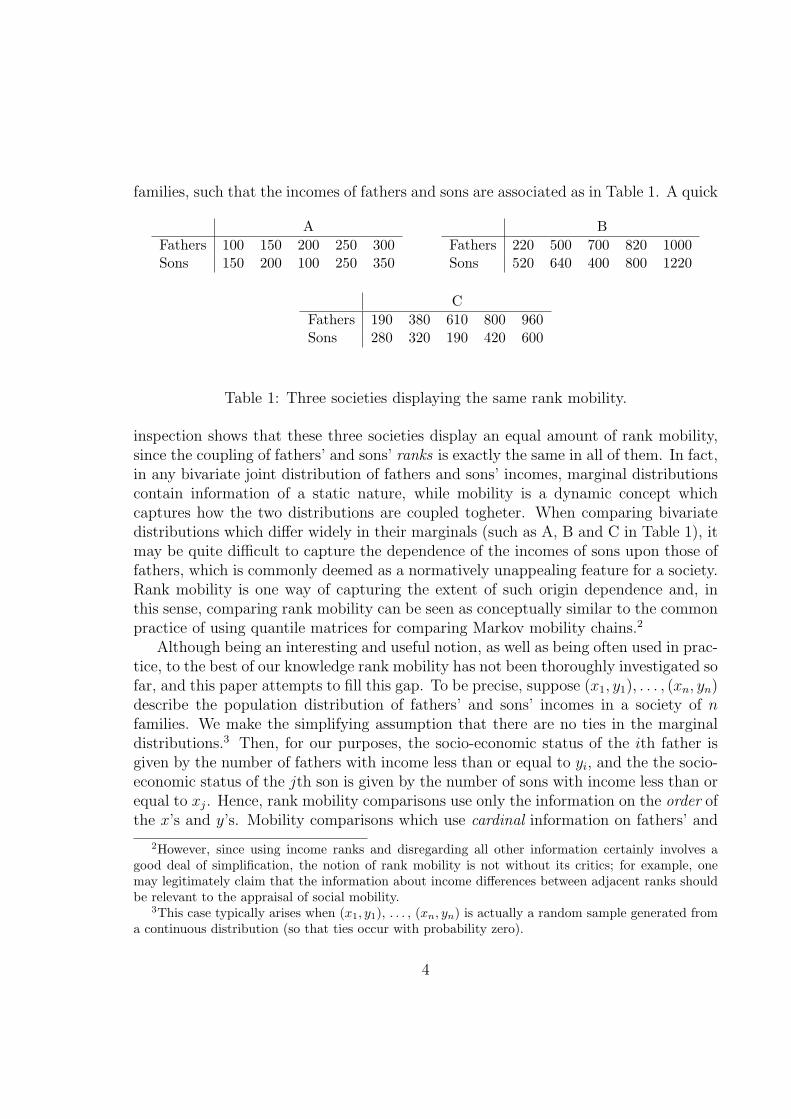
families, such that the incomes of fathers and sons are associated as in Table 1. A quick

AFathers 100 150 200 250 300Sons 150 200 100 250 350

BFathers 220 500 700 820 1000Sons 520 640 400 800 1220

CFathers 190 380 610 800 960Sons 280 320 190 420 600

Table 1: Three societies displaying the same rank mobility.

inspection shows that these three societies display an equal amount of rank mobility,since the coupling of fathers’ and sons’ ranks is exactly the same in all of them. In fact,in any bivariate joint distribution of fathers and sons’ incomes, marginal distributionscontain information of a static nature, while mobility is a dynamic concept whichcaptures how the two distributions are coupled togheter. When comparing bivariatedistributions which differ widely in their marginals (such as A, B and C in Table 1), itmay be quite difficult to capture the dependence of the incomes of sons upon those offathers, which is commonly deemed as a normatively unappealing feature for a society.Rank mobility is one way of capturing the extent of such origin dependence and, inthis sense, comparing rank mobility can be seen as conceptually similar to the commonpractice of using quantile matrices for comparing Markov mobility chains.2

Although being an interesting and useful notion, as well as being often used in prac-tice, to the best of our knowledge rank mobility has not been thoroughly investigated sofar, and this paper attempts to fill this gap. To be precise, suppose (x1, y1), . . . , (xn, yn)describe the population distribution of fathers’ and sons’ incomes in a society of nfamilies. We make the simplifying assumption that there are no ties in the marginaldistributions.3 Then, for our purposes, the socio-economic status of the ith father isgiven by the number of fathers with income less than or equal to yi, and the the socio-economic status of the jth son is given by the number of sons with income less than orequal to xj. Hence, rank mobility comparisons use only the information on the order ofthe x’s and y’s. Mobility comparisons which use cardinal information on fathers’ and

2However, since using income ranks and disregarding all other information certainly involves agood deal of simplification, the notion of rank mobility is not without its critics; for example, onemay legitimately claim that the information about income differences between adjacent ranks shouldbe relevant to the appraisal of social mobility.

3This case typically arises when (x1, y1), . . . , (xn, yn) is actually a random sample generated froma continuous distribution (so that ties occur with probability zero).

4

sons’ income are axiomatized, among others, by [4, 5, 10, 12, 16, 20, 22, 24, 26] andcapture different aspects of social mobility than the present paper. These contributionsmay be considered more complementary than alternative to our approach. Fields ([9],chapter 6) compares some theoretical properties of various indices of income mobilityincluding some indices of rank mobility such as rank correlation, and Buchinsky et al.[3] compare their empirical properties in an application to French income mobility.4

Given our assumption of no ties in the marginal distributions, all the informationconcerning the rank mobility of a society is contained in a permutation matrix P ,with typical element P (i, j) equal to 1 if there is a family in this society whose fatherhas rank i and son has rank j, and 0 otherwise. The problem is how to turn thisinformation into a quantitative measure.5 In order to achieve a faithful and consistentrepresentation of the rank mobility of subgroups within a given society, we address theproblem in terms of partial permutation matrices (defined in Section 2) which includestandard (“global”) matrices as a special case, and argue that a representation of therank mobility of a given subgroup of the population in terms of global matrices would beparadoxical. After observing that a standard decomposability property — which is keyin the characterization of additively separable indices — cannot be sensibly assumedin the context of measuring rank mobility, we take advantage of our representationin terms of partial matrices to define a weaker form of decomposability which canbe safely assumed. As an intermediate step, in section 3 we provide (Theorem 1) acharacterization of a partial ordering on partial matrices which in the case of globalmatrices coincides with the well-known “concordance” ordering.

We then provide (in Theorems 2 and 3) a rather natural and simple characteriza-tion (up to a monotonic transformation) of an index of rank mobility based on partialmatrices and show that, in the standard case of comparing the mobility of two globalmatrices of equal size, this is equivalent to Spearman’s ρ index. We also discuss (inProposition 2 and 1) another interesting incomplete preorder which lies between con-cordance and the class of its completions (over partial matrices of equal size) singledout by Theorem 2. We finally show, in the last section, how the characterized index canbe naturally extended to one which provides a complete preorder of partial matrices ofdifferent size. Our results seem to provide reasonable grounds for adopting this kind ofindex (rather than other alternative ones, such as Kendall’s τ or Spearman’s footrule)in the measurement of rank mobility.

4The only characterization of a mobility index which takes explicit account of ranks that we areaware of is [20]. King’s index uses information not only on the ranks of fathers’ and sons’ incomes,but also on their numerical values, and thus his approach in not directly conparable with ours, butcan be considered complementary.

5Note that if (x1, y1), . . . , (xn, yn) is a random sample and we multiply by 1n the permutation

matrix P we obtain the so called empirical joint rank distribution function (see Block et al. [2]).

5

2 Subgroup mobility and partial permutation ma-

trices

Let F denote the set of all families who live in a given society and consider a subsetA ⊆ F ; examples of interesting subsets are the families which live in a given geo-graphical location, or which belong to a given ethnic group, or whose fathers have agiven education level etc. Sometimes we may be interested in exploring how the statusof individuals change from one generation to the next for members of this particularsubset. We could call this kind of information the rank mobility of A with respect toF . Observe that this is not the same as considering the rank mobility of A w.r.t.A, because individuals’ rank is calculated with respect to the whole of F . A simpleexample may help to clarify. Consider a society F consisting of six families in whichthe distributions of fathers’ and sons’ incomes is summarized in Table 2 below:

1 2 3 4 5 6Fathers 100 150 200 250 300 350Sons 150 200 100 250 350 300

Table 2: Incomes of fathers and sons in F .

Now, consider the subset A of F consisting only of the third, fourth and fifth families.If we consider only A and calculate the rank of individuals with respect to this specificsubset, then there is no rank mobility from one generation to the next. Viceversa,there is clearly a sense in which the families in A exhibit some status mobility, whichis made apparent when the status is calculated with respect to the whole of F : the sonof the third family has lost two positions with respect to his generation, while the sonof the fifth family has gained one position.

This kind of “partial” mobility information, i.e. restricted to a subset of a wholeset F of families, will then be described by an n × n matrix which differs from apermutation matrix because it can have rows and columns with zeros only. Suchmatrices are called partial permutation matrices.6 When necessary for clarity, we shallcall ordinary permutation matrices global. More formally, the set Pn of n × n partialpermutation matrices is defined as follows: a matrix P belongs to Pn if and only if, forall i = 1, . . . , n and j = 1, . . . , n, we have: (i) P (i, j) ∈ {0, 1}; (ii)

∑i P (i, j) ≤ 1; (iii)∑

j P (i, j) ≤ 1. Notice that, under this definition, global matrices are nothing but aspecial case of partial matrices.

Now, suppose A and B are disjoint subsets of a set F of n families. Clearly thepartial permutation matrices that describe the rank mobility of A and B with respect

6See e.g. Horn and Johnson [17] for definitions and some properties of partial permutation matrices.

6

to F , call them P and Q, will belong to Pn and will be disjoint in a related sense thatis expressed by the following definition:

Definition 1. P,Q ∈ Pn are disjoint if

P (i, j) = 1 and Q(m, k) = 1⇒ i 6= m and j 6= k.

Corollary 1. P,Q ∈ Pn are disjoint if and only if P + Q ∈ Pn, where + is the usualsum of matrices.

Therefore, the rank mobility with respect to F of disjoint subsets of F is representedby disjoint partial matrices. Notice that if we partition F into m mutually exclusiveand exhaustive subsets A1, . . . , Am, the rank mobility of these subsets with respect toF will be described by mutually disjoint partial matrices P1, . . . , Pm such that P =P1 + · · ·+ Pm. Let us say that a partial matrix P is atomic if there exists exactly onei and one j such that P (i, j) = 1, that is, if we are considering a subset containingexactly one family. We shall use the lower case letter p (possibly with subscripts) todenote atomic matrices. Clearly, any partial permutation matrix in Pn will be equalto a sum p1 + · · ·+ pk of k ≤ n atomic matrices, where k = n only for global matrices.

Observe that any n× n partial matrix P can be regarded as representing the rankmobility of some set of families A with respect to some “society” F of size n thatincludes it. Indeed, it is always possible to find an F such that the rank mobilitydetermined by the marginal distributions of fathers’ and sons’ income is representedby a global matrix that includes P . So, the above corollary implies that the sum oftwo disjoint partial matrices can always be regarded as representing the rank mobilityof some suitable subgroup A of a possible “society” F . Therefore, in this abstractsetting, we can forget about “real” families, groups and societies and concentrate onlyon the partial matrices that represent their rank mobility. However, to avoid long-winded sentences, we shall often abuse of the more concrete terminology and speak,for instance, of “a society (group) P” to mean “a society (group) whose rank mobilityis represented by the (partial) matrix P”, or of “the family (i, j) (in a matrix P )” tomean “the family in which the father’s rank is i and the son’s rank is j (in a societywhose rank mobility is represented by P )”.

We are interested in investigating the properties of some suitable ordering � overthe class P =

⋃∞i=1Pi such that P � Q can be taken as meaning that the matrix Q

exhibits at least the same degree of social mobility as the matrix P .

3 Axiomatizing rank mobility orderings

In this section we shall start investigating the ordering relation �, by restricting ourattention to comparisons between matrices of equal size. In other words, the charac-

7

terized orderings will be such that P � Q holds true only if both P and Q belongto the same subclass Pn for some fixed n. We shall sometimes use the notation �n

for the restriction of � to Pn, but will omit the subscript n whenever it is clear fromthe context that we are comparing matrices of the same size. Then, in Section 4 weshall discuss how � can be extended in a natural way into a rank mobility index whichapplies to all partial matrices (of arbitrary size), so inducing a complete preorder overthe whole class P .

Given two matrices P and Q in Pn (for some given n), when can we say that Qdisplays at least the same rank mobility as P? We first introduce and discuss someplausible axioms to impose on the ordering� and then derive characterization theoremsfollowing an incremental approach. As a first step, in Section 3.1, we shall only assumethat � is a preorder, that is a reflexive and transitive binary relation. Then, we shallderive, in Theorem 1, a characterization of what we propose as the basic rank mobilityordering from two axioms. Such ordering allows only for comparisons between partialmatrices of equal size which satisfy the further condition of being “similar” (in thesense explained in Definition 2) and is not complete on any of the classes Pn. Next, inSection 3.2, we shall investigate possible extensions of this basic preorder. Assumingthat, for all n, �n is a complete preorder of Pn, we shall introduce further axioms whichwill allow us to obtain sharper characterizations in Theorems 2 and 3.

3.1 The concordance ordering

While it is intuitively clear that it is meaningful to compare two standard (i.e. global)permutation matrices representing the rank mobility of two societies F and F ′, itis not quite as clear whether it is equally meaningful to compare partial matrices —representing, say, the rank mobility of some subsetA ∈ F w.r.t. F and the rank mobilityof some subset B ∈ F ′ w.r.t. F ′ — when they have different marginal distributions.7

We shall therefore start by restricting the comparison to a clear-cut case.

Definition 2. We say that:

1. Two matrices P,Q ∈ Pn are similar if

{i|P (i, j) = 1 for some j} = {i|Q(i, j) = 1 for some j} and

{j|P (i, j) = 1 for some i} = {j|Q(i, j) = 1 for some i}.

2. A matrix P ∈ Pn is monotone if, for all i, j,m, k such that P (i, j) = 1 andP (m, k) = 1, we have (i−m)(j − k) > 0.

7Loosely speaking, by “marginal distributions” of a partial matrix P we mean the following: themarginal distribution of the fathers is the set of all i such that P (i, j) = 1 for some j, and the marginaldistribution of the sons is the set of all j such that P (i, j) = 1 for some i.

8

So, two matrices are similar when they have equal marginal distributions. Note that thedefinition of similarity induces an equivalence relation on Pn. Moreover, observe thatwithin each similarity set there is a unique monotone matrix which can be consideredas displaying the least amount of mobility:

Axiom 1 (Monotonicity). For all n, and for all distinct P,Q ∈ Pn such that P ismonotone and similar to Q we have P ≺ Q.

Notice also that a matrix is monotone if, and only if, there is a strictly increasingfunction from fathers’ rank to sons’ rank.8

The second axiom requires that the sum of disjoint partial matrices is a monotonicoperation:

Axiom 2 (Subgroup Consistency). For all n and for every P1, P2, P3, P4 ∈ Pn suchthat P1 is disjoint with P2 and P3 is disjoint with P4

P1 � P3 and P2 � P4 ⇒ P1 + P2 � P3 + P4.

Similar axioms are commonly used in the literature on income inequality [28],poverty [15] and mobility measurement [12],9 where they usually imply a fundamen-tal, and practically useful, decomposability property: given an arbitrary partition of apopulation into k subgroups, the problem of measuring a certain feature in the overallpopulation can be reduced to the k separate problems of measuring that feature in eachof the k subgroups.10 It must be stressed that the above axiom cannot be interpretedas asserting a similar decomposability of the rank mobility of a society F into the rankmobility of their subgroups. In the terminology used in the introduction, this wouldamount to asserting that, given a partition of F into A1, . . . , Ak, the rank mobility of Fw.r.t. F , can be decomposed into the rank mobility of A1 w.r.t. A1, A2 w.r.t. A2, etc.,where the rank of each individual is evaluated with reference to the subgroup to whichit belongs. However, this would clearly be paradoxical in the context of measuringrank mobility.

To see why, recall the simple example given in Section 2 (see Table 2), considering asociety made of six families. Let A1 be the subgroup consisting of the third, fourth and

8The reader may find it helpful to compare our concept of similar matrices with the well-knownFrechet class of distributions with fixed marginals, and our monotonicity axiom with the lower boundin the Frechet class (see e.g. Nelsen [25]).

9Though such axioms are widely accepted in these contexts, for a critical discussion see Foster andSen [14].

10For this interpretation of the decomposability property in the context of social mobility see,for instance, Fields and Ok [10]. The term decomposability has different interpretations in othertheoretical and applied contexts.

9

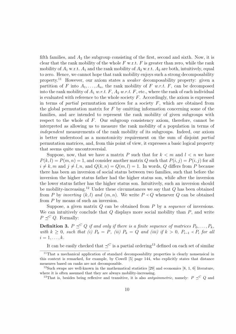
fifth families, and A2 the subgroup consisting of the first, second and sixth. Now, it isclear that the rank mobility of the whole F w.r.t. F is greater than zero, while the rankmobility of A1 w.r.t. A1 and the rank mobility of A2 w.r.t. A2 are both, intuitively, equalto zero. Hence, we cannot hope that rank mobility enjoys such a strong decomposabilityproperty.11 However, our axiom states a weaker decomposability property: given apartition of F into A1, . . . , An, the rank mobility of F w.r.t. F , can be decomposedinto the rank mobility of A1 w.r.t. F , A2 w.r.t. F , etc., where the rank of each individualis evaluated with reference to the whole society F . Accordingly, the axiom is expressedin terms of partial permutation matrices for a society F , which are obtained fromthe global permutation matrix for F by omitting information concerning some of thefamilies, and are intended to represent the rank mobility of given subgroups withrespect to the whole of F . Our subgroup consistency axiom, therefore, cannot beinterpreted as allowing us to measure the rank mobility of a population in terms ofindependent measurements of the rank mobility of its subgroups. Indeed, our axiomis better understood as a monotonicity requirement on the sum of disjoint partialpermutation matrices, and, from this point of view, it expresses a basic logical propertythat seems quite uncontroversial.

Suppose, now, that we have a matrix P such that for k < m and l < n we haveP (k, l) = P (m,n) = 1, and consider another matrix Q such that P (i, j) = P (i, j) for alli 6= k,m and j 6= l, n, and Q(k, n) = Q(m, l) = 1. In words, Q differs from P becausethere has been an inversion of social status between two families, such that before theinversion the higher status father had the higher status son, while after the inversionthe lower status father has the higher status son. Intuitively, such an inversion shouldbe mobility-increasing.12 Under these circumstances we say that Q has been obtainedfrom P by inverting (k, l) and (m,n). We write P � Q whenever Q can be obtainedfrom P by means of such an inversion.

Suppose, a given matrix Q can be obtained from P by a sequence of inversions.We can intuitively conclude that Q displays more social mobility than P , and writeP �C Q. Formally:

Definition 3. P �C Q if and only if there is a finite sequence of matrices P0, . . . , Pk,with k ≥ 0, such that (i) P0 = P , (ii) Pk = Q and (iii) if k > 0, Pi−1 � Pi for alli = 1, . . . , k.

It can be easily checked that �C is a partial ordering13 defined on each set of similar

11That a mechanical application of standard decomposability properties is clearly nonsensical inthis context is remarked, for example, by Cowell [5] page 144, who explicitly states that distancemeasures based on ranks are not decomposable.

12Such swaps are well-known in the mathematical statistics [29] and economics [8, 1, 6] literature,where it is often assumed that they are always mobility-increasing.

13That is, besides being reflexive and transitive, it is also antysimmetric, namely: P �C Q and

10

matrices. The reason for the choice of the superscript “C” is that, when the similarityclass consists of the global matrices in Pn, �C is called the concordance ordering inthe mathematical statistics literature, see e.g. Tchen [29] and Kimeldorf and Sampson[19].

Theorem 1. Within each set of similar matrices, �C is the smallest14 preorder whichsatisfies Axiom 1 and Axiom 2.

A proof of this theorem is given in Appendix A. The concordance ordering �C is avery well established and much studied ordering of bivariate distributions. It is a partialordering which, in the space of global permutation matrices, is a subrelation of manyimportant complete orders, for example, those induced by the popular nonparametricindices of concordance such as Kendall’s τ and Spearman’s ρ, see e.g. Schweizer andWolff [27]. The theorem then says that all reflexive and transitive relations � whichsatisfy Axioms 1 and 2 must have a common area of agreement equal to �C . Atkin-son [1] first applies the concordance ordering to mobility measurement; Dardanoni [6]applies it to a Markov chain model of social mobility, and shows the equivalence of aversion of this ordering to some very intuitive concepts of greater social mobility. Inparticular, appropriately defining father’s and sons’ status as monotonic functions oftheir rank, Theorem 4 of Dardanoni [6] can be adapted to this context to show theequivalence of �C with useful partial orderings for making rank mobility comparisonsin ways that parallel the classical Lorenz ordering.

On the other hand, �C allows for comparisons between similar matrices only and,while this restriction is immaterial when comparing global matrices, it makes the com-parison of partial matrices impossible except for the artificial special case in which thematrices have exactly the same marginal distributions. Moreover, being a partial or-dering, �C does not even allow for comparisons of all matrices in a given similarity set.Thus, in order to be able to compare all mobility contexts in Pn (for any n), we mustfocus on preorders � such that every restriction �n is a complete preorder of Pn.15

Clearly, even assuming that each �n is complete, Axioms 1 and 2 are not sufficient toprovide a unique characterization (since these axioms are satisfied by several distinctpreorders which are complete on every Pn, e.g. the above mentioned ρ and τ .) Fromthis point of view, Theorem 1 only implies that every preorder which is complete oneach Pn and satisfies the axioms must include �C , so that the properties expressedby the axioms can be considered as minimal requirements on any suitable mobilityordering. Thus, in the sequel, we shall take our mobility ordering � to be a complete

Q �C P imply that P = Q.14In terms of set-inclusion.15Recall that �n is a complete preorder of Pn when for all P,Q ∈ Pn, either P �n Q or Q �n P .

11

preorder of each Pn and seek for extra axiomatic properties that allow us to uniquelycharacterize it.

3.2 Completing the concordance ordering

In this section we investigate the possible completions over each Pn of the basic con-cordance ordering characterized in Theorem 1. We shall therefore assume that eachrestriction �n of our mobility ordering � is a complete preorder of Pn and considerthe class of such preorders satisfying Axioms 1 and 2. (As implied by Theorem 1, theymust all include the concordance ordering.) Our aim, now, is to investigate how theseaxioms can be expanded to single out a suitable mobility ordering from this class.

There are two distinct intuitive aspects of the notion of “greater mobility” whichemerge from its conceptual analysis. One aspect, which is apparent in the standarddefinitions of some well-known orderings — such as the concordance ordering and thecomplete preorder based on Kendall’s function τ — stems from the idea that there isan increase in mobility when two families interchange their relative position. On theother hand, from a different angle, mobility is related to the distance between father’sand sons’s status within each family, and overall mobility of a group of families maybe construed as the aggregation of the degrees of mobility exhibited by all the familiesin that group.16

Now, for a single family in a society F , such that father’s rank is i and son’s rank isj, we can take |i− j| as measuring the social distance between father’s and son’s socialstatus. This basic intuition is captured by the following:

Axiom 3 (Atomic Monotonicity). For all n and for any two atomic matrices p, q ∈ Pn

such that p(i, j) = q(i′, j′) = 1,

p � q ⇐⇒ |i− j| ≤ |i′ − j′|.

Notice that, although this axiom forces a unique complete preorder of atomic matrices,it is not sufficient to uniquely characterize �n in the whole domain of Pn. It shouldalso be noted17 that this axiom forces one to care about rank alterations only as far asthe extent of these alterations is concerned, disregarding where these alterations occur.For example, this axiom forces one to see an equal amount of mobility in an atomicpermutation matrix in which father’s rank is the worst and son’s rank is one above theworst, and in an atomic permutation matrix in which father’s rank is the second best

16Clearly these two concepts of mobility (one which considers the interplay of families and the otherwhich considers families in isolation) are interrelated, since single families cannot change relativepositions without affecting other families.

17We thank a referee for pointing this out to us.

12

and son’s rank is the best. One may find this objectionable from a normative point ofview, for lower income dynamics are often deemed more important from this angle. Onthe other hand, it can be observed that such concerns appear to be more significantwhen considering the difference between father’s and son’s actual income, rather thanbetween their rank. Clearly, the same amount of income movement may appear to bemore significant as the level of income decreases, but it is not obvious that the sameshould hold true for movement of ranks, since in this case all the information concerningthe actual income levels is discarded. It may well be that the actual movement ofincome oberved within a low rank family is much smaller than the one observed withina high rank family. Since any purely ordinal approach simply discards this kind ofinformation, it is not obviuos how to assign higher weight to lower income dynamics.

Let’s now introduce some notation which will simplify considerably the followingdiscussion. If “P” denotes a matrix in a given space Pn, then “Pm”, with m ≥ n, willdenote the matrix in Pm which coincides with P wherever P is defined and containsonly 0’s everywhere else, i.e. the matrix defined as follows:

Pm(i, j) = P (i, j) for all i, j ≤ n and

Pm(i, j) = 0 otherwise.

On the other hand, if “P” denotes a matrix in Pm, we shall attach no meaning to thenotation “P k” with k < m. Observe that, by definition,

1. (P k)m = Pm for every m ≥ k

2. (P +Q)m = Pm +Qm for every disjoint P,Q ∈ Pk with k ≤ m.

Let us say that a matrix P is null if i = j for all (i, j) such that P (i, j) = 1. Intuitively,a null-matrix says that the subgroup for which it is defined displays no mobility at all.The following axiom is an adaptation of the well-known Archimedean Property to oursetting:

Axiom 4 (Archimedean Property). For every m and all P,Q ∈ Pm, the strict inequal-ity P ≺ Q holds if and only if there is an n ≥ m and a non-null R ∈ Pn, disjoint withP n, such that

P n +R ∼ Qn.

The meaning of this axiom is that there is no gap between the mobility displayed by twopartial matrices (groups of families) which cannot be bridged if one takes into accountthe possibility that the societies in which these are embedded are expanded. That is,if the total number of families is increased and the group displaying less mobility isexpanded with new families which display positive mobility, it is always possible toequalize the mobility of the other group.

13

It must be stressed that such an axiom is acceptable only if one is concerned withthe absolute amount of mobility displayed by the partial matrices, disregarding anyconsideration of the size of the groups whose mobility they represent.18 To intuitivelygrasp this axiom one can usefully compare it with a similar property which holds inthe field of real numbers, where p < q holds true if and only if there is a positive rsuch that p + r = q. In fact, this axiom could be taken as a definition of the relationP ≺ Q, once it has been made clear that this relation concerns absolute rank mobilitycomparisons.

Observe now that, within a given class Pn, a partial permutation matrix P isuniquely determined by the set S(P ) = {(i, j)|P (i, j) = 1}. We call S(P ) the charac-teristic set of P . We can prove the following:

Theorem 2. Let � be a preorder over P such that �n is complete over Pn for everyn ∈ N. Then � satisfies Axioms 1–4 if and only if there is a strictly increasing andstrictly convex function f : N→ N such that, for all n and for all P,Q ∈ Pn,

P � Q⇐⇒∑

(i,j)∈S(P )

f(|i− j|) ≤∑

(i,j)∈S(Q)

f(|i− j|). (1)

A proof of this theorem is given in Appendix B. Theorem 2 shows that Axioms 1–4characterize (up to a monotonic transformation) a class of additive mobility indiceswhich depend on the choice of an appropriate weighting function f . It is interesting tonotice that, within the space of global matrices, two important indices of ordinal asso-ciation which would seem appropriate to (im)mobility measurement, namely Kendall’sτ and Spearman’s footrule (see e.g. Kendall and Gibbons [18] for definitions and adiscussion of their properties) do not belong to the class defined in Theorem 2.

Consider for example the global permutation matrices P , P ′ and P ′′ in P4 with thefollowing characteristic sets:

S(P ) = {(1, 1), (2, 4), (3, 3), (4, 2)}S(P ′) = {(1, 3), (2, 1), (3, 4), (4, 2)},S(P ′′) = {(1, 1), (2, 3), (3, 4), (4, 2)}.

Using any of the mobility indices, say M , in the class characterized by Theorem 2, themobility of P , P ′ and P ′′ will be equal to

M(P ) = H(f(0) + f(2) + f(0) + f(2)

),

M(P ′) = H(f(2) + f(1) + f(1) + f(2)

),

M(P ′′) = H(f(0) + f(1) + f(1) + f(2)

)18On the other hand, a “relative” notion of rank mobility, which takes into account the size of

the groups, can be soundly based on the absolute notion outlined in this section. On this point seeSection 4 below.

14

for some strictly increasing and strictly convex f and strictly increasing H. Now, ifwe adopted Spearman’s footrule as a mobility measure, which corresponds to letting fbe the identity function, P and P ′′ would display the same amount of mobility, since0 + 2 + 0 + 2 = 0 + 1 + 1 + 2. However, P can be derived from P ′′ by an inversion of thefamilies (2, 3) and (3, 4). Thus P ′′ ≺C P , and so Spearman’s footrule is inconsistentwith �C . This failure of Spearman’s footrule to satisfy the basic ordering �C makesit unsuitable for measuring rank mobility.

On the other hand, it is easy to show that, in the class of global matrices, Kendall’sτ does indeed agree with �C (see e.g. Schweizer and Wolff [27]). Nevertheless, it cannotsatisfy all our axioms, as can be seen by observing that P and P ′ have the same valueof Kendall’s τ , while any of the indices of Theorem 2 would deliver different values,since in P ′ there are two families with social distance equal to 2 (as in P ), but, inaddition, there are also two families with positive social distance (since f is strictlyincreasing).

Now, Theorem 2 characterizes a class of complete preorders of each Pn which, whilebeing small enough to exclude some important mobility indices, is still too wide andits practical application is dependent on the choice of an appropriate function f . Atthis stage a natural option, suggested by a referee, is to look for a preorder which seeksagreement in equivalence (1) for all strictly increasing and strictly convex functionsf : N → N.19 Let dP denote the vector of rank differences |i − j|’s for the families inS(P ), with dimension equal to the cardinality of S(P ), and let dP denote the decreasingrearrangement of dP . Standard results in the stochastic dominance literature20 implythe following:

Proposition 1. For all n and for all P,Q ∈ Pn such that |S(P )| = |S(Q)| = k ≤ n,the following conditions are equivalent:

1.∑

(i,j)∈S(P ) f(|i− j|) ≤∑

(i,j)∈S(Q) f(|i− j|) for all strictly increasing and strictlyconvex function f : N→ N;

2.∑j

i=1 dPi ≤

∑ji=1 d

Qi , j = 1, . . . , k.

Proposition 1 gives an empirically verifiable condition which is equivalent to theagreement in equivalence (refsumoff) for all strictly increasing and strictly convex func-tions f . Let us �M be the preorder defined by Condition 2 of Proposition 1 above,

19The axiomatic characterization of a preorder which seeks agreement in equivalence (1) for allstrictly increasing and strictly convex functions f is an intersting topic for future research. Someinspiration may come from the work of Dubra, Maccheroni and Ok [7], who characterize an expectedutility representation for a potentially incomplete preference relation over lotteries by means of a setof von Neumann-Morgenstern utility functions.

20In particular, applying Marshall and Olkin’s [[23] Theorem 3.C.1.b] on weak submajorization,using the techniques of Fishburn and LaValle [13] who investigate stochastic dominance on grids.

15

which is defined on any P,Q ∈ Pn (for some fixed n) with the same number of non-zeroentries. The following proposition shows that, within each class of similar matrices,�M is in fact an extension of �C :

Proposition 2. For all n and for all similar P,Q ∈ Pn, P �C Q implies P �M Q butthe converse does not apply.

A proof that, within each class of similar matrices, �C implies �M is in Appendix C.That the converse is not true can be established by the following example: let P be theglobal matrix in P3 with carachteristic set S(P ) equal to {(1, 2), (2, 1), (3, 3)}, and let Qbe the global matrix in P3 with carachteristic set S(Q) equal to {(1, 1), (2, 3), (3, 2)}.Then dP = (1, 1, 0) and dQ = (0, 1, 1), so that dP = dQ. Therefore, Condition 2 ofProposition 1 applies and P ∼M Q, but it can be easily checked that P and Q are notcomparable by �C .

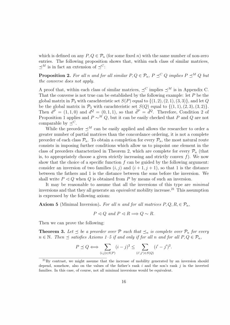
While the preorder �M can be easily applied and allows the researcher to order agreater number of partial matrices than the concordance ordering, it is not a completepreorder of each class Pn. To obtain a completion for every Pn, the most natural routeconsists in imposing further conditions which allow us to pinpoint one element in theclass of preorders characterized in Theorem 2, which are complete for every Pn (thatis, to appropriately choose a given strictly increasing and strictly convex f). We nowshow that the choice of a specific function f can be guided by the following argument:consider an inversion of two families (i, j) and (i + 1, j + 1), so that 1 is the distancebetween the fathers and 1 is the distance between the sons before the inversion. Weshall write P C Q when Q is obtained from P by means of such an inversion.

It may be reasonable to assume that all the inversions of this type are minimalinversions and that they all generate an equivalent mobility increase.21 This assumptionis expressed by the following axiom:

Axiom 5 (Minimal Inversion). For all n and for all matrices P,Q,R,∈ Pn,

P C Q and P C R =⇒ Q ∼ R.

Then we can prove the following:

Theorem 3. Let � be a preorder over P such that �n is complete over Pn for everyn ∈ N. Then � satisfies Axioms 1–5 if and only if for all n and for all P,Q ∈ Pn,

P � Q⇐⇒∑

(i,j)∈S(P )

(i− j)2 ≤∑

(i′,j′)∈S(Q)

(i′ − j′)2.

21By contrast, we might assume that the increase of mobility generated by an inversion shoulddepend, somehow, also on the values of the father’s rank i and the son’s rank j in the invertedfamilies. In this case, of course, not all minimal inversions would be equivalent.

16

A proof is given in Appendix D. It can be easily verified that, within the set of globalmatrices, Theorem 3 characterizes (up to a monotonic transformation) the well-knownSpearman index of ordinal association, since the latter (which is better described asan immobility index) can be written as

ρ(P ) = 1−6∑

(i,j)∈S(P )(i− j)2

n3 − n(see e.g. Kendall and Gibbons [18], page 8).

On the other hand, the ordering characterized in Theorem 3 is not restricted topopulations’ comparisons. For partial permutation matrices, the theorem provides ameans for comparing the status mobility of different subgroups when the concept ofsocial status we are interested in refers to the rank of individuals in the whole society.As an example, recall again the society F considered in in Section 2 (see Table 2), andassume that the third, fourth and fifth family belong to a first group, while the first,second and sixth belong to a second group. It is then easily calculated that families inthe first group exhibit a greater level of rank mobility than those in the second; since,applying Theorem 3, we have 4 + 0 + 1 > 1 + 1 + 1.

4 A rank mobility index

Theorem 3 provides a characterization of a preorder �, which is complete over eachclass Pn consisting of all partial matrices of a given fixed size n. However, in manysituations it would be useful to go beyond the preorder �, since:

• when comparing two matrices, say P and Q, we may want to conclude not onlythat P displays more rank mobility than Q, but also to be able to claim in ameaningful way that, say, P displays 20% more mobility than Q;

• the characterized ordering allows us to compare matrices of the same size ina meaningful way, but it is of no use when it comes to comparing matrices ofdifferent size. Thus, it would be desirable to be able to compare partial matricesover the set P =

⋃∞i=1Pn of partial matrices of any size;

• � allows us to compare all partial matrices of the same size n, and so to comparethe overall rank mobility of arbitrary subgroups, regardless of the number of fam-ilies (i, j) composing the subgroup. Although this may be intuitively sound whenone is interested in measuring the absolute amount of rank mobility exhibited bya subgroup, alternatively one may be interested in a relative notion of mobilitywhich takes into account the number of families which compose the subgroupswhich are being compared.

17

Let then In : Pn 7→ R be a rank mobility index implicitely characterized by Theo-rem 3:

In(P ) = Fn

( ∑(i,j)∈S(P )

(i− j)2)

where Fn is some strictly increasing function. A first reasonable property to impose onIn(P ) is that Fn is in fact a similarity transformation, that is,

In(P ) = cn( ∑

(i,j)∈S(P )

(i− j)2)

for some positive constant cn. If we now let I : P 7→ R denote a rank mobilityindex which allows comparisons of all matrices in P , it is then natural to assume that,whenever P ∈ Pn, I(P ) = In(P ).

A further property that one may wish to impose on such a rank mobility indexI is that it achieves a fixed maximum, which can be conventionally chosen to be 1,and this maximum is reached by any “antimonotone” partial matrix. In particular,let Ak,n ∈ Pn denote the partial matrix such that (i) the cardinality of S(Ak,n) is k(that is, Ak,n contains k families), and (ii) families’ ranks are as folows: (1, n), (2, n−1), ..., (k, n − k + 1). It can then be argued that, among all partial matrices P ∈ Pn

with S(P ) having cardinality k, Ak,n displays the maximum amount of mobility, thatis, for any k and n, I(Ak,n) = 1. It then immediately follows that the rank mobilityindex we seek has the following form:

I(P ) =1

(k3 − k)/3 + k(n− k)2

∑(i,j)∈S(P )

(i− j)2

for any partial matrix P ∈ Pn with cardinality of S(P ) equal to k. Notice that toderive the index above we have used the fact that, for any Ak,n,

∑(i,j)∈S(Ak,n)(i− j)2 =

(k3 − k)/3 + k(n− k)2.Two properties of our rank mobility index I may be worth noticing. First, the

index actually measures the percentage of rank mobility (measured according to theformula characterized in Theorem 3) of any given partial matrix P with respect to thetheoretically maximum achievable rank mobility for a subgroup with the same numberof families in a society of the same size. Secondly, when P is a global matrix (thatis, k = n), it is immediately checked that I coincides with Spearman’s index ρ, afterallowing for the fact that Spearman’s index range is [−1, 1] while I(P ) ∈ [0, 1] and, asremarked above, ρ measures immobility rather than mobility.

18

Appendices

A Proof of Theorem 1

Proof. We first show that the �C ordering (which, we recall, is defined on each set ofsimilar partial matrices) satisfies the axioms. It is obvious that it satisfies Axiom 1.As for Axiom 2, suppose P1, P2 and P3, P4 are mutually disjoint, and P1 �C P3 andP2 �C P4. Then there exists a sequence Q0, . . . , Qk of partial matrices in Pn such that(i) Q0 = P1, (ii) Qk = P3 and, whenever k > 0, (iii) Qi � Qi+1 for i = 0, . . . , k − 1.Similarly, there exists a sequence R0, . . . , Rk′ of partial matrices in Pn such that (i)R0 = P2, (ii) Rk′ = P4 and, whenever k′ > 0, (iii) Ri � Ri+1 for i = 0, . . . , k′ − 1.Suppose k′ > k. Then, it is easy to see that, since P1, P2, and P3, P4 are mutuallydisjoint, the sequence

Q0 +R0, . . . , Qk +Rk, Qk +Rk+1, . . . , Qk +Rk′

is such that (i) Q0 +R0 = P1 +P2, (ii) Qk +Rk′ = P3 +P4, (iii) Qi +Ri �Qi+1 +Ri+1

for i = 0, . . . , k − 1, and (iv) Qk + Rj � Qk + Rj+1 for j = k, . . . , k′ − 1. Hence, bydefinition of �C , we have that P1 + P2 �C P3 + P4. The argument is similar whenk > k′.

Next, we show that if a preorder � satisfies the axioms, then it must include theconcordance ordering. This is sufficient to conclude that �C is the smallest preordersatisfying the axioms.

Suppose � satisfies the axioms. Let P and Q be two matrices such that P �C Q.By definition, this means that P and Q are similar and there is a sequence of matricesP0, . . . , Pk, with k ≥ 0, such that P0 = P , Pk = Q and, if k > 0, Pi � Pi+1 for all i =1, . . . , k−1. Now consider the i-th inversion step, and suppose it is such that, for somej,m, l, n with j < m and l < n, Pi−1(j, l) = Pi−1(m,n) = 1 and Pi(j, n) = Pi(m, l) = 1.Consider the matrix P ∗i−1 such that only P ∗i−1(j, l) = P ∗i−1(m,n) = 1, while all the otherentries are 0 (that is, its characteristic set S(P ∗i−1) is equal to {(j, l), (m,n)}). Let alsoP ∗i be the similar matrix such that only P ∗i (j, n) = P ∗i (m, l) = 1, while all the otherentries are 0 (that is, its characteristic set S(P ∗i ) is equal to {(j, n), (m, l)}).

ClearlyPi−1 = (Pi−1 − P ∗i−1) + P ∗i−1 and Pi = (Pi − P ∗i ) + P ∗i .

Moreover, Pi−1 − P ∗i−1 = Pi − P ∗i and, since j < m and l < n, the matrix P ∗i−1 is amonotone matrix, so that P ∗i−1 � P ∗i (by Axiom 1). Therefore,

Pi−1 = (Pi−1 − P ∗i−1) + P ∗i−1 � (Pi − P ∗i ) + P ∗i = Pi

by Axiom 2. Hence, Pi−1 � Pi. The same argument holds for all i, therefore P � Q.This shows that P �C Q implies P � Q for all P,Q, i.e. �C is included in �. Since

19

� was an arbitrary preorder satisfying the axioms, �C is included in all the preorderssatisfying the axioms.

B Proof of Theorem 2

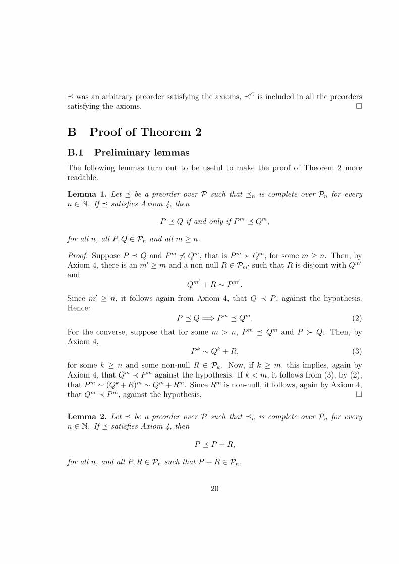
B.1 Preliminary lemmas

The following lemmas turn out to be useful to make the proof of Theorem 2 morereadable.

Lemma 1. Let � be a preorder over P such that �n is complete over Pn for everyn ∈ N. If � satisfies Axiom 4, then

P � Q if and only if Pm � Qm,

for all n, all P,Q ∈ Pn and all m ≥ n.

Proof. Suppose P � Q and Pm 6� Qm, that is Pm � Qm, for some m ≥ n. Then, byAxiom 4, there is an m′ ≥ m and a non-null R ∈ Pm′ such that R is disjoint with Qm′

andQm′

+R ∼ Pm′.

Since m′ ≥ n, it follows again from Axiom 4, that Q ≺ P , against the hypothesis.Hence:

P � Q =⇒ Pm � Qm. (2)

For the converse, suppose that for some m > n, Pm � Qm and P � Q. Then, byAxiom 4,

P k ∼ Qk +R, (3)

for some k ≥ n and some non-null R ∈ Pk. Now, if k ≥ m, this implies, again byAxiom 4, that Qm ≺ Pm against the hypothesis. If k < m, it follows from (3), by (2),that Pm ∼ (Qk +R)m ∼ Qm +Rm. Since Rm is non-null, it follows, again by Axiom 4,that Qm ≺ Pm, against the hypothesis.

Lemma 2. Let � be a preorder over P such that �n is complete over Pn for everyn ∈ N. If � satisfies Axiom 4, then

P � P +R,

for all n, and all P,R ∈ Pn such that P +R ∈ Pn.

20

Proof. Suppose P � P +R. Then, by Axiom 4,

Pm ∼ (P +R)m + S ∼ Pm +Rm + S

for some m ≥ n and some non-null S ∈ Pm. Since Rm + S is non-null, this wouldimply, again by Axiom 4, that P � P , which is impossible.

Let us denote by ⊥n the unique matrix P ∈ Pn, that we call the empty matrix, suchthat P (i, j) = 0 for all i, j, that is the n×n matrix which is everywhere undefined. Bydefinition, (i) ⊥n is a null matrix (ii) for every P ∈ Pn, ⊥n is disjoint with P , and (iii)⊥n + P = P .

Lemma 3. Let � be a preorder over P such that �n is complete over Pn for everyn ∈ N. If � satisfies Axioms 2, 3 and 4, then

⊥n ∼ P ≺ Q

for every null matrix P ∈ Pn and every non-null matrix Q in Pn.

Proof. First, recall that (by Axiom 4) ⊥n ≺ Q, for every n and every non-null Q ∈ Pn,since ⊥n + Q = Q ∼ Q. Hence, we only have to show that P ∼ ⊥n for every nullP ∈ Pn. If P = ⊥n, then it is trivially true that P ∼ ⊥n. Consider, then, the case thatP 6= ⊥n. Let us first show that p ∼ ⊥n for every null atomic matrix p in Pn. Suppose,that p � ⊥n. Then, by Axiom 4, pm ∼ ⊥m +R = R for some m ≥ n and some non-nullR ∈ Pm. Since R is non-null, R = r + T for some non-null atomic matrix r and some,possibly null, matrix T in Pm. By Axiom 3, pm ≺ r and, by Lemma 2, pm ≺ r+T = R.This is a contradiction, since we had before concluded that pm ∼ R. Suppose, then,that ⊥n � p. By Axiom 4, pm +R ∼ ⊥m for some m ≥ n and some non-null R ∈ Pm.Now, since ⊥m ≺ Q for every non-null Q ∈ Pm, it follows that ⊥m ≺ R. Then, byLemma 2, ⊥m ≺ pm + R against the previous conclusion that ⊥m ∼ pm + R. Hence,since � is a complete preorder of Pm, ⊥m ∼ p.

If P is not an atomic matrix and P 6= ⊥n, then P = p1 + · · ·+ pk for some k suchthat 1 < k ≤ n, with each pi (1 ≤ i ≤ k) being a null atomic matrix. As we havejust established, pi ∼ ⊥n for all i = 1, . . . , k. Hence, by Axiom 2 (and recalling that⊥n +⊥n = ⊥n), P ∼ ⊥n.

Say that two matrices P and Q are atomically equivalent if, for every k ≥ 0, theycontain the same number of non-zero entries (i, j) with |i − j| = k. Clearly, if P andQ are atomically equivalent, there are atomic matrices p1, . . . , pm and q1, . . . , qm, withm ≤ n, such that P = p1 + · · · + pm, Q = q1 + · · · + qm and, by Axiom 3, pi ∼ qi fori = 1, . . . ,m. Hence, by Axiom 2, if P and Q are atomically equivalent, then P ∼ Q.

21

Remark 1. Given any two matrices P,Q ∈ Pn, one can always find a sufficientlylarge m and a matrix R in Pm such that R is atomically equivalent to Qm and disjointwith Pm. For this purpose, it is sufficient to take m = 2n and R equal to the matrixsuch that (i) R(i, j) = 0 for all i, j ≤ n and (ii) R(n + i, n + j) = 1 if and only ifQ(i, j) = 1. Using this method, if P1, . . . , Pk are matrices in Pn, one can always findsuitable matrices P ′1, . . . , P

′k ∈ Pkn such that (i) P kn

i ∼ P ′i for i ≤ k and (ii) all the P ′iare mutually disjoint.

Lemma 4. Let � be a preorder over P such that �n is complete over Pn for everyn ∈ N. If � satisfies Axioms 2 and 4, then for all n, and all P,Q,R, S ∈ Pn such thatP is disjoint with R and Q is disjoint with S,

P ∼ Q and P +R ∼ Q+ S =⇒ R ∼ S.

Proof. Let us assume that P ∼ Q and P + R ∼ Q + S. Suppose, ex absurdo, thatR 6∼ S.

Case 1: R � S. Then, it follows from Axiom 4, that Rm ∼ Sm +T for some m ≥ nand some non-null T ∈ Pm. By Remark 1, there are m′ ≥ m and U ∈ Pm′ such thatU ∼ Pm′

and U is disjoint with Sm + T . Hence, by Lemma 1 and Axiom 2,

Pm′+Rm′ ∼ U + Sm′

+ T ∼ Qm′+ Sm′

.

So, by Axiom 4, U + Sm′ ≺ Qm′+ Sm′

(since T is non-null). However, by Axiom 2,U + Sm′ ∼ Qm′

+ Sm′(since U ∼ Pm′ ∼ Qm′

by hypothesis and Lemma 1), which is acontradiction.

Case 2: R ≺ S. This case is similar to Case 1 and is left to the reader.

Now, consider the set P =⋃∞

i=1Pi of all partial matrices. We define the subset ∆k,k ≥ 0, of P as the set of all P ∈ P such that for all (i, j) ∈ S(P ), |i− j| ≤ k. Noticethat ∆k ⊆ ∆m whenever k ≤ m. The matrices in ∆0 are the null matrices. We shallalso write ∆n

k for ∆k ∩ Pn. Moreover, given two matrices P,Q ∈ Pn, let us say that Qis contained in P if P (i, j) = 1 for all i, j ∈ {1, . . . , n} such that Q(i, j) = 1. Recallthat every partial matrix can be uniquely expressed as a sum of atomic matrices.

Lemma 5. Let � be a preorder over P such that �n is complete over Pn for everyn ∈ N. If � satisfies Axioms 2, 3 and 4, then for all n and all P,Q ∈ ∆n

1 , P � Qif and only if the number of non-null atomic matrices contained in P is less than orequal to the number of non-null atomic matrices contained in Q.

Proof. Suppose first that the number of non-null atomic matrices contained in P is lessthan or equal to the number of non-null atomic matrices contained in Q. Let p1, . . . , pj

22

be the non-null atomic matrices in P and q1, . . . , qk the non-null atomic matrices in Q,with j ≤ k ≤ n. Then P = p1+· · ·+pj+R for some null R ∈ Pn and Q = q1+· · ·+qj+Sfor some possibly non-null S ∈ Pn. By Axiom 3 all the non-null atomic matrices in ∆n

1

are equivalent to each other and therefore, by Axiom 2, p1 + · · · + pj ∼ q1 + · · · + qj.Moreover, by Lemma 3, R � S. Hence, again by Axiom 2, P � Q. Suppose now thatthe number of non-null atomic matrices in P is strictly greater than the number ofnon-null atomic matrices in Q. Let p1, . . . , pk the non-null atomic matrices in P andq1, . . . , qj the non-null atomic matrices in Q, with j ≤ k ≤ n. So, P = p1 + · · ·+ pj +Rfor some non-null R ∈ Pn and Q = q1 + · · ·+qj +S for some null S ∈ Pn. Moreover, byLemma 3, S ≺ R and, as argued above, p1 + · · ·+ pj ∼ q1 + · · ·+ qj. So, by Axiom 2,Q = q1 + · · · + qj + S � p1 + · · · + pj + R = P . By Lemma 4, Q ∼ P would implythat S ∼ R which, given that S is null and R is non-null, is ruled out by Lemma 3.Therefore, we can conclude that Q ≺ P .

Lemma 6. Let � be a preorder over P such that �n is complete over Pn for everyn ∈ N. If � satisfies Axioms 2–4, then for every n and every atomic matrix p ∈ Pn,there is an m ≥ n such that pm ∼ Q for some Q ∈ ∆m

1 .

Proof. Since every atomic matrix p ∈ Pn belongs to some ∆nk , with k ∈ N, we prove

the lemma by induction on the index k of the smallest class ∆nk to which p belongs. In

the course of the proof, and for the sake of clarity, we shall reserve the notation P , Q,etc. to refer to matrices in ∆1.

Base: p ∈ ∆n1 . Trivial.

Step: p ∈ ∆nj+1 (j ≥ 1). Assuming that the lemma holds for all atomic matrices

in ∆nj we show that it holds also for all atomic matrices in ∆n

j+1.Suppose p is an atomic matrix which belongs to ∆n

j+1 but does not belong to ∆nj .

Then, p is non-null and, by Axiom 3, all atomic matrices in ∆nj are strictly less than

p. Let now q be a non-null atomic matrix in ∆nj . Then, q ≺ p and, by Axiom 4,

qm + R ∼ pm for some m ≥ n and some non-null R ∈ Pm. Since, qm is itself non-null,this implies (again by Axiom 4) that R ≺ pm. Now, we argue that R must be in ∆m

j .We reason by absurd. Suppose R 6∈ ∆m

j , then R = r + S for some atomic r ∈ Pm notin ∆m

j , and some (possibly empty) matrix S ∈ Pm. However (by Axiom 3) r � pm and(by Lemma 2) r + S � pm. Hence, R � pm against the conclusion, reached before,that R ≺ pm. Thus, R must be in ∆m

j and so also qm + R is in ∆mj . By inductive

hypothesis, there is an m′ ≥ m such that qm′+ Rm′ ∼ P for some P ∈ ∆m′

1 . So, sincepm ∼ qm +R, by Lemma 1, pm′ ∼ P . This concludes the proof of the lemma.

23

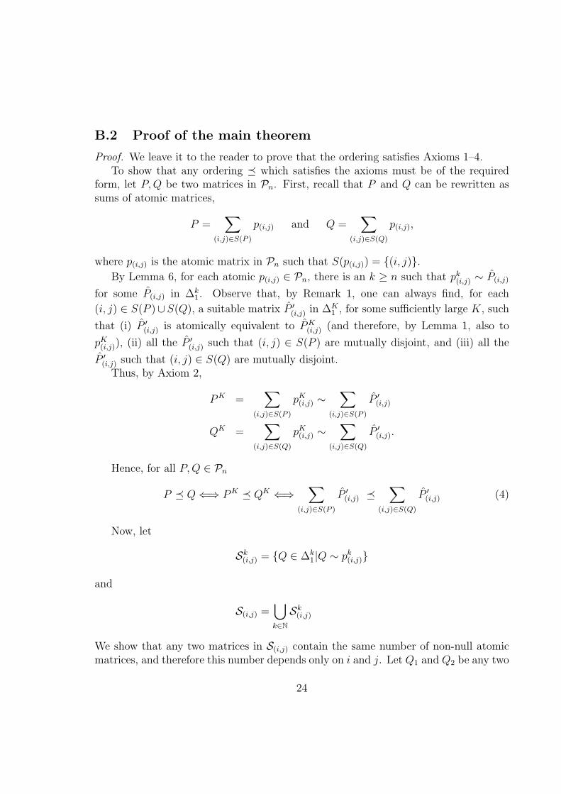
B.2 Proof of the main theorem

Proof. We leave it to the reader to prove that the ordering satisfies Axioms 1–4.To show that any ordering � which satisfies the axioms must be of the required

form, let P,Q be two matrices in Pn. First, recall that P and Q can be rewritten assums of atomic matrices,

P =∑

(i,j)∈S(P )

p(i,j) and Q =∑

(i,j)∈S(Q)

p(i,j),

where p(i,j) is the atomic matrix in Pn such that S(p(i,j)) = {(i, j)}.By Lemma 6, for each atomic p(i,j) ∈ Pn, there is an k ≥ n such that pk

(i,j) ∼ P(i,j)

for some P(i,j) in ∆k1. Observe that, by Remark 1, one can always find, for each

(i, j) ∈ S(P )∪S(Q), a suitable matrix P ′(i,j) in ∆K1 , for some sufficiently large K, such

that (i) P ′(i,j) is atomically equivalent to PK(i,j) (and therefore, by Lemma 1, also to

pK(i,j)), (ii) all the P ′(i,j) such that (i, j) ∈ S(P ) are mutually disjoint, and (iii) all the

P ′(i,j) such that (i, j) ∈ S(Q) are mutually disjoint.Thus, by Axiom 2,

PK =∑

(i,j)∈S(P )

pK(i,j) ∼

∑(i,j)∈S(P )

P ′(i,j)

QK =∑

(i,j)∈S(Q)

pK(i,j) ∼

∑(i,j)∈S(Q)

P ′(i,j).

Hence, for all P,Q ∈ Pn

P � Q⇐⇒ PK � QK ⇐⇒∑

(i,j)∈S(P )

P ′(i,j) �∑

(i,j)∈S(Q)

P ′(i,j) (4)

Now, let

Sk(i,j) = {Q ∈ ∆k

1|Q ∼ pk(i,j)}

and

S(i,j) =⋃k∈N

Sk(i,j)

We show that any two matrices in S(i,j) contain the same number of non-null atomicmatrices, and therefore this number depends only on i and j. Let Q1 and Q2 be any two

24

matrices in S(i,j). Then, for some k, k′, Q1 ∈ ∆k1, Q2 ∈ ∆k′

1 , Q1 ∼ pk(i,j) and Q2 ∼ pk′

(i,j).

We assume without loss of generality that k′ ≥ k. By Lemma 1, pk′

(i,j) ∼ Qk′1 , and so

Qk′1 ∼ Q2. Since these two matrices are both in ∆k′

1 , by Lemma 5, they must contain thesame number of non-null atomic matrices. Moreover, the number of non-null atomicmatrices contained in Qk′

1 is the same as the number of those contained in Q1. Thus,all the matrices in the set S(i,j) contain the same number of non-null atomic matriceswhich depends only on i and j. Let us denote it by n(i,j) and let f be the functionN 7→ N such that, for every i, j, f(|i− j|) = n(i,j). So, since P ′(i,j) belongs to S(i,j), the

number of non-null atomic matrices contained in P ′(i,j) is equal to f(|i− j|).Now, the matrices

∑(i,j)∈S(P ) P

′(i,j) and

∑(i,j)∈S(Q) P

′(i,j) in (4) are in ∆K

1 . So, byLemma 5, they can be compared by simply counting the number of non-null atomicmatrices contained in them. This is equal to the sum of the numbers of non-null atomicmatrices contained in each P ′(i,j) which is, in turn, equal to f(|i− j|). Therefore:∑

(i,j)∈S(P )

P ′(i,j) �∑

(i,j)∈S(Q)

P ′(i,j) ⇐⇒∑

(i,j)∈S(P )

f(|i− j|) ≤∑

(i,j)∈S(Q)

f(|i− j|). (5)

Finally, from (4) and (5) it follows that:

P � Q⇐⇒∑

(i,j)∈S(P )

f(|i− j|) ≤∑

(i,j)∈S(Q)

f(|i− j|).

It is obvious, by Axiom 3, that f must be strictly increasing. To show that f must bestrictly convex, consider, for any k ≥ 0, the matrices P and Q such that:

S(P ) = {(1, k + 1), (2, k + 2), (k + 3, k + 3), (k + 4, k + 4), · · · }S(Q) = {(1, k + 2), (2, k + 1), (k + 3, k + 3), (k + 4, k + 4), · · · }.

Hence, by Axiom 1, we must have that, for all k, 2f(k) < f(k + 1) + f(k − 1).

C Proof of Proposition 2

Proof. Within each class of similar matrices, to prove that �C implies �M , givenDefinition 3 and Proposition 1, it suffices to show that for any partial matrices Pand Q such that P � Q, we have

∑ji d

Pi ≥

∑ji d

Qk for all j ≤ k, where k denotes the

number of non-zero entries in P and Q (the cardinality of S(P ) and S(Q)). Now,notice that when P � Q, dP and dQ differ only by two elements, say dP

m 6= dQm and

dPn 6= dQ

n . The result follows since, as it is easily checked, max{dPm, d

Pn } > max{dQ

m, dQn }

and dPm + dP

n ≥ dQm + dQ

n .

25

D Proof of Theorem 3

Proof. Given Theorem 2, we can concentrate only on Axiom 5. The reader can easilycheck that if f(k) = k2 the ordering satisfies Axiom 5.

To show that, in order to satisfy Axiom 5, f must be quadratic, suppose P,Q,Rare matrices in Pn such that:

S(P ) = {(0, 0), (1, 1), (0, k), (1, k + 1)}S(Q) = {(0, 1), (1, 0), (0, k), (1, k + 1)}S(R) = {(0, 0), (1, 1), (0, k + 1), (1, k)}.

Thus, P C Q and P C R, since the inversions that lead from P to Q and from P to Rare both minimal. Then, by Axiom 5, Q ∼ R and therefore:∑(i,j)∈S(Q)

f(|i− j|) = 2f(1) + 2f(k) =∑

(i,j)∈S(R)

f(|i− j|) = 2f(0) + f(k + 1) + f(k − 1).

Observe that, by definition of f , f(0) = 0, and f(1) = 1 (see above, Appendix B.2).Therefore, to satisfy Axiom 5, since k is arbitrary and f is fixed for all n, we must havethat, for all k,

f(k + 1)− f(k) = f(k)− f(k − 1) + 2.

This difference equation has a unique solution, i.e. f(k) = k2.

26

References

[1] A.B. Atkinson. The measurement of economic mobility. In A.B. Atkinson, editor,Social Justice and Public Policy. Wheatsheaf Books Ltd., London, 1983.

[2] H.W. Block, D. Chhetry, Z. Fang, and A.R. Sampson. Partial orders on permuta-tions and dependence orderings on bivariate empirical distributions. The Annalsof Statistics, 18:1840–50, 1990.

[3] M. Buchinsky, G. Fields, D. Fougre, and F. Kramarz. Francs and ranks: Earningsmobility in france, 1967-1999. CEPR Discussion Paper, 9, 2005.

[4] S.R. Chakravarty, Dutta B., and J. A. Weymark. Ethical indices of income mo-bility. Social Choice and Welfare, 2:1–21, 1985.

[5] F. Cowell. Measures of distributional change: An axiomatic approach. Review ofEconomic Studies, 52:35–51, 1985.

[6] V. Dardanoni. Measuring social mobility. Journal of Economic Theory, 61:372–94,1993.

[7] J. Dubra, F. Maccheroni, and E. Ok. Expected utility theory without the com-pleteness axiom. Journal of Economic Theory, 115:118–133, 2004.

[8] L.G. Epstein and S.M. Tanny. Increasing generalized correlation: A definition andsome economic consequences. Canadian Journal of Economics, 13:16–34, 1980.

[9] G. S. Fields. Distribution and Development: A New Look at the Developing World.MIT Press, Boston, 2002.

[10] G.S. Fields and E. Ok. The meaning and measurement of income mobility. Journalof Economic Theory, 71:349–77, 1996.

[11] G.S. Fields and E. Ok. The measurement of income mobility. In J. Silber, ed-itor, Handbook of Income Inequality Measurement. Kluwer Academic Publishers,Dordrecht, 1999.

[12] G.S. Fields and E. Ok. Measuring movements of incomes. Economica, 66:455–71,1999.

[13] P.C. Fishburn and I. H. LaValle. Stochastic dominance on unidimensional grids.Mathematics of Operations Research, 20:513–525, 1995.

27

[14] J.E. Foster and A. Sen. On economic inequality after a quarter century. In A. Sen,editor, On Economic Inequality. Clarendon Press, Oxford, 1997.

[15] J.E. Foster and A.F. Shorrocks. Subgroup consistent poverty indices. Economet-rica, 59:687–709, 1991.

[16] P Gottschalk and E. Spolaore. On the evaluation of economic mobility. Review ofEconomic Studies, 69:191–208, 2002.

[17] R. A. Horn and C. R. Johnson. Topics in Matrix Analysis. CUP, 1991.

[18] M. Kendall and J.D. Gibbons. Rank Correlation Methods. Edward Arnold, 1990.

[19] G. Kimeldorf and A.R. Sampson. Positive dependence orderings. Annals of theInstitute of Statistical Mathematics, 39:113–128, 1987.

[20] M.A. King. An index of ineqaulity: with applications to horizontal equity andsocial mobility. Econometrica, 51:99–116, 1983.

[21] E. Maasoumi. On mobility. In D. Giles and A. Ullah, editors, The Handbook ofEconomic Statistics. Marcel Dekker, New York, 1998.

[22] E. Maasoumi and S. Zandvakili. A class of generalized measures of mobility withapplications. Economics Letters, 22:97–102, 1986.

[23] A. W. Marshall and I. Olkin. Inequalities: Theory of Majorization and Its Appli-cations. Accademic Press, New York, 1979.

[24] T. Mitra and E. Ok. The measurement of income mobility: A partial orderingapproach. Economic Theory, 12:77–102, 1998.

[25] R. B. Nelsen. An Introduction to Copulas. New York: Springer, 1999.

[26] J. Ruiz-Castillo. The measurement of structural and exchange mobility. Journalof Economic Inequality, 2:219–228, 2004.

[27] B. Schweizer and E.F. Wolff. On non-parametric measures of dependence forrandom variables. Annals of Statistics, 9:879–885, 1981.

[28] A.F. Shorrocks. Aggregation issues in inequality measurement. In W. Eichorn,editor, Measurement in Economics. Springer Verlag, New York, 1988.

[29] A.H.T. Tchen. Inequalities for distributions with given marginals. Annals ofProbability, 8:814–27, 1980.

28