Rank Position Forecasting in Car Racing
14
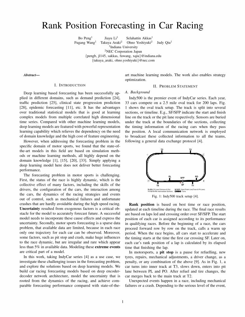
Rank Position Forecasting in Car Racing Bo Peng 1 Jiayu Li 1 Selahattin Akkas 1 Fugang Wang 1 Takuya Araki 2 Ohno Yoshiyuki 2 Judy Qiu 1 1 Indiana University 2 NEC Corporation Japan {pengb, jl145, sakkas, fuwang, xqiu}@indiana.edu {takuya araki, ohno.yoshiyuki}@nec.com Abstract— I. I NTRODUCTION Deep learning based forecasting has been successfully ap- plied in different domains, such as demand prediction [24], traffic prediction [25], clinical state progression prediction [28], epidemic forecasting [11], etc. It has the advantages over traditional statistical models that is good at learning complex models from multiple correlated high dimensional time series. Compared with other machine learning models, deep learning models are featured with powerful representation learning capability which relieves the dependency on the need of domain knowledge and the high cost of feature engineering. However, when addressing the forecasting problem in the specific domain of motor sports, we found that the state-of- the-art models in this field are based on simulation meth- ods or machine learning methods, all highly depend on the domain knowledge [1], [15], [20], [33]. Simply applying a deep learning model here does not deliver better forecasting performance. The forecasting problem in motor sports is challenging. First, the status of the race is highly dynamic, which is the collective effect of many factors, including the skills of the drivers, the configuration of the cars, the interaction among the cars, the dynamics of the racing strategies and events out of control, such as mechanical failures and unfortunate crashes that are hardly avoidable during the high speed racing. Uncertainty resulted from exogenous factors is a critical ob- stacle for the model to accurately forecast future. A successful model needs to incorporate these cause effects and express the uncertainty. Secondly, motor sports forecasting is a sparse data problem, that available data are limited, because in each race only one trajectory for each car can be observed. Moreover, some factors, such as pit stop and crash, make huge influences to the race dynamic, but are irregular and rare which appear less than 5% in available data. Modeling these extreme events are critical part of a model. In this work, taking IndyCar series [4] as a use case, we investigate these challenging issues in the forecasting problem, and explore the solutions based on deep learning models. We build car racing forecasting models based on deep encoder- decoder network architecture, model the uncertainty that is rooted from the dynamics of the racing, and achieve com- parable forecasting performance compared with state-of-the- art machine learning models. The work also enables strategy optimization. II. PROBLEM STATEMENT A. Background Indy500 is the premier event of IndyCar series. Each year, 33 cars compete on a 2.5 mile oval track for 200 laps. Fig. 1 shows the oval track setup. The track is split into several sections, or timeline. E.g., SF/SFP indicate the start and finish line on the track or the pit lane respectively. Sensors are buried under the track at the boundaries of the sections, collecting the timing information of the racing cars when they pass the position. A local communication network is employed to broadcast these collected information to all the teams, following a general data exchange protocol [4]. T3 T2 PO PL T4 T1 SFP SF PL/PO: Pit Lane Entrance & Exit T1-T2-T3-T4: Intermediate Sections SF/SFP: Start-Finish Line(Track & Pit Lane) ①②③④: Turns Fig. 1: Indy500 track setup [4]. Rank position is based on best time or race position, updated at each timeline during the race. The final race results are based on laps led and crossing order over SF/SFP. The start position of each car is assigned according to its performance in qualifying races. Before the beginning of a race, the cars proceed forward row by row on the track, calls a warm up period. When the race begins, all cars start to accelerate and the timing starts at the time the first car crossing SF. Later on, each car’s rank position of a lap is calculated by its elapsed time that finishing the lap. In motorsports, a pit stop is a pause for refuelling, new tyres, repairs, mechanical adjustments, a driver change, as a penalty, or any combination of the above [9]. As in Fig. 1, a car turns into inner track at T3, slows down, enters into pit lane between PL and PO. After refuel and tire changes, the car merges back to the main track at T2. Unexpected events happen in a race, including mechanical failures or a crash. Depending to the serious level of the event, 1
-
Upload
khangminh22 -
Category
Documents
-
view
2 -
download
0
Transcript of Rank Position Forecasting in Car Racing
Rank Position Forecasting in Car RacingBo Peng1 Jiayu Li1 Selahattin Akkas1
Fugang Wang1 Takuya Araki2 Ohno Yoshiyuki2 Judy Qiu11Indiana University
2NEC Corporation Japan{pengb, jl145, sakkas, fuwang, xqiu}@indiana.edu{takuya araki, ohno.yoshiyuki}@nec.com
Abstract—
I. INTRODUCTION
Deep learning based forecasting has been successfully ap-plied in different domains, such as demand prediction [24],traffic prediction [25], clinical state progression prediction[28], epidemic forecasting [11], etc. It has the advantagesover traditional statistical models that is good at learningcomplex models from multiple correlated high dimensionaltime series. Compared with other machine learning models,deep learning models are featured with powerful representationlearning capability which relieves the dependency on the needof domain knowledge and the high cost of feature engineering.
However, when addressing the forecasting problem in thespecific domain of motor sports, we found that the state-of-the-art models in this field are based on simulation meth-ods or machine learning methods, all highly depend on thedomain knowledge [1], [15], [20], [33]. Simply applying adeep learning model here does not deliver better forecastingperformance.
The forecasting problem in motor sports is challenging.First, the status of the race is highly dynamic, which is thecollective effect of many factors, including the skills of thedrivers, the configuration of the cars, the interaction amongthe cars, the dynamics of the racing strategies and eventsout of control, such as mechanical failures and unfortunatecrashes that are hardly avoidable during the high speed racing.Uncertainty resulted from exogenous factors is a critical ob-stacle for the model to accurately forecast future. A successfulmodel needs to incorporate these cause effects and express theuncertainty. Secondly, motor sports forecasting is a sparse dataproblem, that available data are limited, because in each raceonly one trajectory for each car can be observed. Moreover,some factors, such as pit stop and crash, make huge influencesto the race dynamic, but are irregular and rare which appearless than 5% in available data. Modeling these extreme eventsare critical part of a model.
In this work, taking IndyCar series [4] as a use case, weinvestigate these challenging issues in the forecasting problem,and explore the solutions based on deep learning models. Webuild car racing forecasting models based on deep encoder-decoder network architecture, model the uncertainty that isrooted from the dynamics of the racing, and achieve com-parable forecasting performance compared with state-of-the-
art machine learning models. The work also enables strategyoptimization.
II. PROBLEM STATEMENT
A. BackgroundIndy500 is the premier event of IndyCar series. Each year,
33 cars compete on a 2.5 mile oval track for 200 laps. Fig.1 shows the oval track setup. The track is split into severalsections, or timeline. E.g., SF/SFP indicate the start and finishline on the track or the pit lane respectively. Sensors are buriedunder the track at the boundaries of the sections, collectingthe timing information of the racing cars when they passthe position. A local communication network is employedto broadcast these collected information to all the teams,following a general data exchange protocol [4].
T3 T2
POPL
T4 T1
SFP
SF
PL/PO: Pit Lane Entrance & ExitT1-T2-T3-T4: Intermediate Sections
SF/SFP: Start-Finish Line(Track & Pit Lane)①②③④: Turns
Fig. 1: Indy500 track setup [4].
Rank position is based on best time or race position,updated at each timeline during the race. The final race resultsare based on laps led and crossing order over SF/SFP. The startposition of each car is assigned according to its performancein qualifying races. Before the beginning of a race, the carsproceed forward row by row on the track, calls a warm upperiod. When the race begins, all cars start to accelerate andthe timing starts at the time the first car crossing SF. Later on,each car’s rank position of a lap is calculated by its elapsedtime that finishing the lap.
In motorsports, a pit stop is a pause for refuelling, newtyres, repairs, mechanical adjustments, a driver change, as apenalty, or any combination of the above [9]. As in Fig. 1, acar turns into inner track at T3, slows down, enters into pitlane between PL and PO. After refuel and tire changes, thecar merges back to the main track at T2.
Unexpected events happen in a race, including mechanicalfailures or a crash. Depending to the serious level of the event,
1
sometimes it leads to a dangerous situation for other cars tocontinue the racing with high speed on the track. In thesecases, a full course yellow flag raises to indicate the raceentering a caution laps mode, in which all the cars slow downand follow a safety car and can not overtake until an othergreen flag raised.
B. Rank position forecasting problem and challenges
Rank CarId Lap LapTime
TimeBehindLeader
LapStatus
TrackStatus
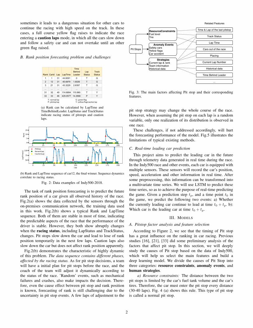
1 1 31 44.6091 0 T G2 12 31 45.6879 1.6026 T G3 21 31 43.3229 2.6397 T G... ... ... ... ... ... ...31 32 49 114.6894 115.965 T Y33 33 46 429.0577 14.2668 P Y
T : normal lap P : pitstop lap
G : green flagY : yellow flag/caution lap
(a) Rank can be calculated by LapTime andTimeBehindLeader. LapStatus and TrackStatusindicate racing status of pitstops and cuationlaps.
0 25 50 75 100 125 150 175 2000
5
10
15
Rank
0 25 50 75 100 125 150 175 200Lap
50
75
100
LapT
ime(
s)
PitStopNoramlLapCautionLap
(b) Rank and LapTime sequence of car12, the final winner. Sequence dynamicscorrelate to racing status.
Fig. 2: Data examples of Indy500-2018.
The task of rank position forecasting is to predict the futurerank position of a car given all observed history of the race.Fig.2(a) shows the data collected by the sensors through theon-premises communication network, the training data usedin this work. Fig.2(b) shows a typical Rank and LapTimesequence. Both of them are stable in most of time, indicatingthe predictable aspects of the race that the performance of thedriver is stable. However, they both show abruptly changeswhen the racing status, including LapStatus and TrackStatus,changes. Pit stops slow down the car and lead to lose of rankposition temporarily in the next few laps. Caution laps alsoslow down the car but does not affect rank position apparently.
Fig.2(b) demonstrates the characteristic of highly dynamicof this problem. The data sequence contains different phases,affected by the racing status. As for pit stop decisions, a teamwill have a initial plan for pit stops before the race, and thecoach of the team will adjust it dynamically according tothe status of the race. ’Random’ events, such as mechanicalfailures and crashes, also make impacts the decision. There-fore, even the cause effect between pit stop and rank positionis known, forecasting of rank is still challenging due to theuncertainty in pit stop events. A few laps of adjustment to the
Pit Stops
ResourceConstraintsFuel levelTire
Anomaly EventsSafety carsYellow flagsCar accident
StrategiesCurrent lap & rankTeam informationHistorical data
Related Features
Time & Lap of the last pitstop
Track Status
Placing
Current Lap Number
Cars out of the race
Historical data
Time Behind Leader
...
Lap Time
Fig. 3: The main factors affecting Pit stop and their correspondingfeatures.
pit stop strategy may change the whole course of the race.However, when assuming the pit stop on each lap is a randomvariable, only one realization of its distribution is observed inone race.
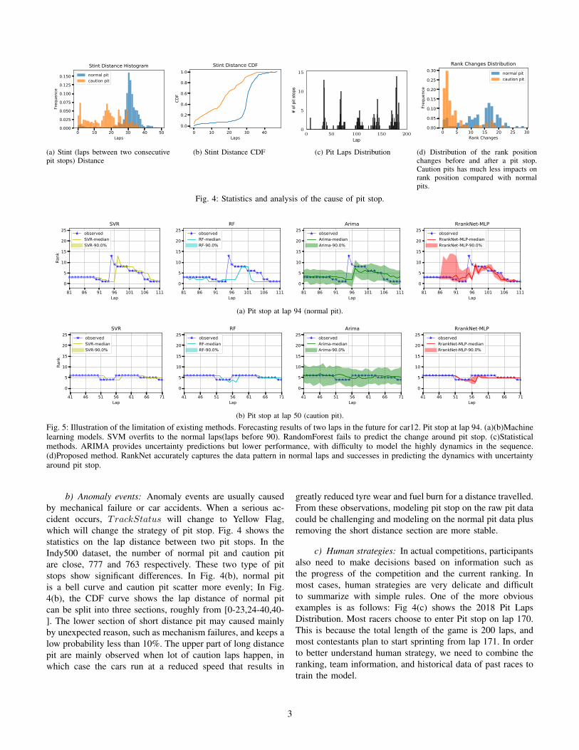
These challenges, if not addressed accordingly, will hurtthe forecasting performance of the model. Fig.5 illustrates thelimitations of typical existing methods.
C. Real-time leading car prediction
This project aims to predict the leading car in the futurethrough telemetry data generated in real time during the race.In the Indy500 race and other events, each car is equipped withmultiple sensors. These sensors will record the car’s position,speed, acceleration and other information in real time. Aftersome preprocessing, this information can be transformed intoa multivariate time series. We will use LSTM to predict thesetime series, so as to achieve the purpose of real-time predictingthe game. Given a prediction step tp, and a time point t0 inthe game, we predict the following two events: a) Whetherthe currently leading car continue to lead at time t0 + tp. b):Which car is the leading car at time t0 + tp.
III. MODELS
A. Pitstop factor analysis and feature selection
According to Figure 2, we see that the timing of Pit stophas a great influence on the ranking in car racing. Previousstudies [16], [21], [33] did some preliminary analysis of thefactors that affect pit stop. In this section, we will deeplystudy the causes of Pit stop based on the data of Indy500,which will help us select the main features and build adeep learning model. We divide the causes of Pit Stop intothree categories: resource constraints, anomaly events, andhuman strategies.
a) Resource constraints: The distance between the twopit stops is limited by the car’s fuel tank volume and the car’stires. Therefore, the car must enter the pit stop every distance(30-40 laps). Fig. 4 (a) shows this rule. This type of pit stopis called a normal pit stop.
2
0 10 20 30 40 50Laps
0.000
0.025
0.050
0.075
0.100
0.125
0.150
Freq
uenc
e
Stint Distance Histogramnormal pitcaution pit
0 10 20 30 40Laps
0.0
0.2
0.4
0.6
0.8
1.0
CDF
Stint Distance CDF
(a) Stint (laps between two consecutivepit stops) Distance
0 10 20 30 40 50Laps
0.000
0.025
0.050
0.075
0.100
0.125
0.150
Freq
uenc
eStint Distance Histogramnormal pitcaution pit
0 10 20 30 40Laps
0.0
0.2
0.4
0.6
0.8
1.0
CDF
Stint Distance CDF
(b) Stint Distance CDF
0 50 100 150 2000
5
10
15
Lap
#of
pits
tops
(c) Pit Laps Distribution
0 5 10 15 20 25 30Rank Changes
0.00
0.05
0.10
0.15
0.20
0.25
0.30
Freq
uenc
e
Rank Changes Distributionnormal pitcaution pit
(d) Distribution of the rank positionchanges before and after a pit stop.Caution pits has much less impacts onrank position compared with normalpits.
Fig. 4: Statistics and analysis of the cause of pit stop.
81 86 91 96 101 106 111Lap
0
5
10
15
20
25
Rank
observedSVR-medianSVR-90.0%
SVR
81 86 91 96 101 106 111Lap
0
5
10
15
20
25 observedRF-medianRF-90.0%
RF
81 86 91 96 101 106 111Lap
0
5
10
15
20
25 observedArima-medianArima-90.0%
Arima
81 86 91 96 101 106 111Lap
0
5
10
15
20
25 observedRrankNet-MLP-medianRrankNet-MLP-90.0%
RrankNet-MLP
(a) Pit stop at lap 94 (normal pit).
41 46 51 56 61 66 71Lap
0
5
10
15
20
25
Rank
observedSVR-medianSVR-90.0%
SVR
41 46 51 56 61 66 71Lap
0
5
10
15
20
25 observedRF-medianRF-90.0%
RF
41 46 51 56 61 66 71Lap
0
5
10
15
20
25 observedArima-medianArima-90.0%
Arima
41 46 51 56 61 66 71Lap
0
5
10
15
20
25 observedRrankNet-MLP-medianRrankNet-MLP-90.0%
RrankNet-MLP
(b) Pit stop at lap 50 (caution pit).
Fig. 5: Illustration of the limitation of existing methods. Forecasting results of two laps in the future for car12. Pit stop at lap 94. (a)(b)Machinelearning models. SVM overfits to the normal laps(laps before 90). RandomForest fails to predict the change around pit stop. (c)Statisticalmethods. ARIMA provides uncertainty predictions but lower performance, with difficulty to model the highly dynamics in the sequence.(d)Proposed method. RankNet accurately captures the data pattern in normal laps and successes in predicting the dynamics with uncertaintyaround pit stop.
b) Anomaly events: Anomaly events are usually causedby mechanical failure or car accidents. When a serious ac-cident occurs, TrackStatus will change to Yellow Flag,which will change the strategy of pit stop. Fig. 4 shows thestatistics on the lap distance between two pit stops. In theIndy500 dataset, the number of normal pit and caution pitare close, 777 and 763 respectively. These two type of pitstops show significant differences. In Fig. 4(b), normal pitis a bell curve and caution pit scatter more evenly; In Fig.4(b), the CDF curve shows the lap distance of normal pitcan be split into three sections, roughly from [0-23,24-40,40-]. The lower section of short distance pit may caused mainlyby unexpected reason, such as mechanism failures, and keeps alow probability less than 10%. The upper part of long distancepit are mainly observed when lot of caution laps happen, inwhich case the cars run at a reduced speed that results in
greatly reduced tyre wear and fuel burn for a distance travelled.From these observations, modeling pit stop on the raw pit datacould be challenging and modeling on the normal pit data plusremoving the short distance section are more stable.
c) Human strategies: In actual competitions, participantsalso need to make decisions based on information such asthe progress of the competition and the current ranking. Inmost cases, human strategies are very delicate and difficultto summarize with simple rules. One of the more obviousexamples is as follows: Fig 4(c) shows the 2018 Pit LapsDistribution. Most racers choose to enter Pit stop on lap 170.This is because the total length of the game is 200 laps, andmost contestants plan to start sprinting from lap 171. In orderto better understand human strategy, we need to combine theranking, team information, and historical data of past races totrain the model.
3

TABLE I: Summary of features used in the model
Feature Domain Description SourceLapT ime(N,L) R+ The time it took for car # N to complete lap L. [3]
LapDistance(N,T ) R+ The distance of car # N from the starting line at time T . (Availablefor year 2017 - 2018)
PitstopLap N(List) A list of the laps where car # N entered the pitstop. [3]Rank(N,L) N There are Rank(N,L) cars that completed lap L before car # N [2]Placing(N,T ) N At time t, there are Placing(N, t) cars in front of car N. [3]TrackStatus(N,L) {0, 1} Status of each lap for a car #N, normal lap or caution lap. [2]T imeBehindLeader(N,L) R+ Time behind the leader of car #N in lap #L. [2]
CautionLaps(N,L) N At Lap L, the count of caution laps since the last Pit Lap of carN .
PitAge(N,L) N At lap L, the count of laps after the previous pit stop of car N .CarID {0, 1}33 Categorical car ID
B. Modeling uncertainty in high dynamic sequences
We treat the rank position forecasting as a sequence-to-sequence modeling problem with the assumption that thereare enough information contained in the history to forecastthe future. An encoder-decoder architecture is employed tomap a input sequence zi,1:t to the output sequence zi,t+1:t+k.To modeling the uncertainty, we follow the idea proposed in[29] to deliver probabilistic forecasting. Instead of predictingvalue of target variable in the output sequence directly, aprobabilistic forecasting network predicts all parameters θ(e.g., mean and variance) of the probability distribution. Afixed distribution p(zi,t|θi,t) is parameterized by the output ofthe network hi,t.
We use zi,t to denote the value of time series i at time t, xi,tto represent the covariate that are assumed to be known at anygiven time. Our goal is to model the conditional distribution
P (zi,t0:T |zi,1:t0−1,xi,1:T )
We assume that our model distributionQΘ(zi,t0:T |zi,1:t0−1,xi,1:T ) consists of a product of likelihoodfactors
QΘ(zi,t0:T |zi,1:t0−1,xi,1:T ) =
T∏t=t0
QΘ(zi,t|zi,1:t−1,xi,1:T )
=
T∏t=t0
p(zi,t|θ(hi,t,Θ))
(1)parametrized by the output hi,t of an autoregressive recur-
rent network
hi,t = h(hi,t−1, zi,t−1,xi,t,Θ)
where h is a function that is implemented by a multi-layerrecurrent neural network with LSTM cells parametrized byΘ.
a) Training: The training process is divided into thefollowing steps:
1) At each time step t, input the covariate xi,t, the valueof the previous time step zi,t−1, and the state hi,t−1
of the previous time step. Calculate the current statehi,t = h(hi,t−1, zi,t−1,xi,t) through the neural network.
2) Calculate the parameter θi,t = θ(hi,t) of the likelihoodp(z|θ).
3) Maximize the log-likelihood:
L =
N∑i=1
T∑t=t0
log p(zi,t|θ(hi,t))
b) Prediction: After the training is completed, historicaldata is fed into the network to obtain the initial state. Thenancestral sampling is used to obtain the prediction results. Theprediction phase is divided into the following steps
1) As shown in Fig. 5(b), an independent PitModel is usedto predict the covariates xt+1:t+k.
2) Input the historical data at time step t < t0 into thenetwork to obtain the initial state hi,t0−1.
3) For time steps t, t + 1, ...T , randomly sample at eachtime step to obtain sample zi,t ∼ p(·|θi,t). E.g., for aGaussian distribution,
p(z|µ, σ) = (2πσ2)−1/2 exp(−(z − µ)2/(2σ2)) (2)
This sampled value is used as the input for the next timestep.
4) Repeat step 3 to get a series of z samples. These sampledvalues can be used to calculate the desired target values,such as quantiles, expectations, etc.
Encoder-decoder architecture provides an advantage by sup-porting to incorporate covariates known in the forecastingperiod. For example, in sales demand forecasting, holidays areknown to be important factors to achieve good predictions.These variables can be expressed as covariates inputs intoboth the encoder network and decoder network. As we know,caution laps and pit stops are important factors to the rankposition, therefore, can be considered as covariate inputs. But,different from the holidays, these variables in the future areunknown at the time of forecasting, leading to the need ofdecomposing the cause effects in building the model.
C. Modeling extreme events and cause effects decomposition
Changes of race status, including pit stops and caution laps,cause the phase changes of the rank position sequence. As a di-rect solution to address this cause effect, we can model the racestatus and rank position together and joint train the model in
4

Rank Model(c)
Pit Model(b) Xt+1:t+k
Zt+2
Historical racestatusTrackStatusLapStatusCarIdCautionLapsPitAge ...
Predicted racestatus
RankLapTimeTimeBehindLeader
PredictedRank
Input Data
(a) Process of forecasting. History data first feed intoPitModel to get RaceStatus in the future, then feedinto RankModel to get Rank forecasting. The outputof the models are samples drawed from the learneddistribution.
StackedDense
Dense
Xt+1:t+k
X1:t
θ't
(b) PitModel is a MLP predictingnext pit stop lap given features ofRaceStatus history.
Xt+2
StackedLSTM
Dense
StackedLSTM
Dense
...
Z1
Encoder
Zt
StackedLSTM
Dense
StackedLSTM
Dense
Zt+1 Zt+2
Z0X1
Zt-1Xt
Decoder
ZtXt+1
Zt+1
...
h1
θ1
ht
θt
ht+1 ht+2
Observed
Predicted
Sampling P(Z|θ)
Z
θt+1 θt+2
RankLapTime
TimeBehindLeaderX
TrackStatusLapStatusCarId
Rank Race status
CautionLapsPitAge
(c) RankModel is stacked 2-layers LSTM encoder-decoderpredicting rank for next prediction len laps, given features ofhistorical Rank and RaceStatus, and future RaceStatus predictedby PitModel.
Fig. 6: RankNet architecture.
TABLE II: Dataset statistics and model parameters
# of time series 231Granularity LapDomain R+Encoder length 40Decoder length 2# of training examples 32KItem input embedding dimension 57Item output embedding dimension 30Batch size 32Optimizer ADAMLearning rate 1e-3# of lstm layers 2# of lstm nodes 40Running time 2h
the encoder-decoder network. In this case, target variable zi,tis a multivariate vector [Rank, LapStatus, TrackStatus].However, this method fails in practice due to data sparsity.The changes of race status are rare events, and targets of rareevents require different complexity of models. For example,on average a car goes to pit stop for six times in a race.Therefore, LapStatus, a binary vector with length equals to200, contains only six ones, 3% effect data. When a longlength of context for rank position encoder is necessary, pitstops are more like a first order Markov chain, i.e., the nextpitstop mainly depends on the previous one rather than theones further in the history. TrackStatus, indicating the crashevents, is even harder to predict.
We propose to decompose the cause effect of race status andrank position in the model. RankNet, as shown in Fig. 6(a),is composed with two sub-models. First, a PitModel forecaststhe future RaceStatus, in which LapStatus is predicted andTrackStatus is set to zeros assuming no caution laps inthe future. Then the RankModel forecasts the future Ranksequence.
Target variable Zt is not limited to Rank, it can be any vari-able that enables the calculation of the rank position, includ-ing: the rank position(Rank), time spend for a lap(LapTime),time behind the leader in a lap(TimeBehindLeader). Rank,as observed, is discrete variable which means its value lost
subtle performance differences among the cars. LapTime canaccurately reflect the performance of the race, but needs toaccumulate from the first lap into elapsed time when calculatethe rank position, and may suffer from accumulating error.The last one, TimeBehindLeader, indicates rank directly andcontains correlated information across the cars.
RaceStatus is the most important feature in covariates Xt.TrackStatus indicates whether the current lap is a caution lap,in which the car follows a safety car in controlled speed.LapStatus indicates whether the current lap is a pit stop lap, inwhich the car cross SF/SFP in the pit lane. Some other staticfeatures can also be added into the input. For example, CarIdrepresents the skill level of the driver and performance of thecar.
Transformations are applied on these basic features to gener-ate new features. Embedding for categorical CarId is utilized.Accumulation sum transforms the binary status features into’age’ features, generating features such as CautionLapsandPitAge. Table I summarizes the definition of these features.For efficiency, instead of sequences input and output, PitModelin Fig.6(b) use CautionLaps and PitAge as input, and outputa scalar of the lap number of the next pit stop.
A rank position forecasting network is trained with afixed prediction length. In order to deliver a variable lengthprediction, e.g., in predicting the rank positions between twopit stops, we apply a fixed length forecasting regressively byusing previous output as input for the next prediction.
IV. EXPERIMENTS
A. Dataset
We evaluate our model on the car racing data of IndyCarseries [2]. The timing and score log data covers all the raceevents of IndyCar series from 2008 to 2020. Take 2018 as anexample, which contains 17 events, six of them are racing onthe oval speedway.
One of the challenges in forecasting car racing is datascarcity, because only one trajectory of each car was observedin each race. We have to incorporate more similar data to learn
5

TABLE III: Short-term rank position forecasting(prediction leghth=2)
Dataset Indy500-2018 Indy500-2019Model Top1Acc MAE 50-Risk 90-Risk Top1Acc MAE 50-Risk 90-RiskCurRank 0.72 1.34 0.097 0.097 0.73 1.16 0.080 0.080ARIMA 0.68 2.63 0.097 0.087 0.57 2.25 0.082 0.075RandomForest 0.51 1.75 0.127 0.127 0.62 1.33 0.092 0.092SVM 0.72 1.34 0.097 0.097 0.73 1.18 0.080 0.080XGBoost 0.46 1.63 0.118 0.118 0.64 1.25 0.086 0.086DeepAR 0.66 2.07 0.156 0.096 0.59 1.71 0.121 0.075RankNet-Joint 0.73 1.75 0.140 0.086 0.68 1.63 0.116 0.073RankNet-MLP 0.77 1.24 0.086 0.077 0.78 1.07 0.072 0.061RankNet-Oracle 0.85 1.11 0.080 0.073 0.86 0.98 0.067 0.061
TABLE IV: Short-term rank position forecasting(prediction leghth=2) of Indy500-2019
Dataset Normal lap Lap with eventsModel SignAcc MAE 50-Risk 90-Risk SignAcc MAE 50-Risk 90-RiskCurRank 0.95 0.11 0.01 0.01 0.60 1.86 0.13 0.13RandomForest 0.80 0.38 0.03 0.03 0.51 1.93 0.13 0.13SVM 0.95 0.11 0.01 0.01 0.59 1.86 0.13 0.13XGBoost 0.79 0.23 0.02 0.02 0.55 1.92 0.13 0.13RankNet-MLP 0.93 0.17 0.01 0.01 0.67 1.67 0.11 0.09RankNet-Oracle 0.93 0.17 0.01 0.01 0.81 1.50 0.10 0.09
TABLE V: Rank position changes forecasting between pit stops
Dataset Indy500-2018 Indy500-2019Model SignAcc MAE 50-Risk 90-Risk SignAcc MAE 50-Risk 90-RiskCurRank 0.10 4.15 0.259 0.234 0.15 4.33 0.280 0.262RandomForest 0.57 3.55 0.222 0.221 0.51 4.31 0.277 0.276SVM 0.61 3.42 0.214 0.212 0.51 4.22 0.270 0.249XGBoost 0.49 4.10 0.256 0.234 0.45 4.86 0.313 0.304RankNet-MLP 0.68 3.83 0.240 0.163 0.62 4.33 0.286 0.223RankNet-Oracle 0.71 3.28 0.207 0.189 0.66 3.62 0.234 0.215
a stable model. Using the historical data that are too long timeago can be inefficient because many factors changes along thetime, including the skills of the drivers, configurations of thecars and even the rules of the race. The same year data ofother races are ’similar’ in the status of the drivers, cars andrules, but different length of the track leads to different racingdynamics. In this paper, we use the data of the same event,Indy500, from 2013 to 2019, with the data from 2013 to 2017as training set and the other two years as test set.
B. Implementation and baselines
We build our model RankNet with the Gluonts framework[13]. Gluonts is a library for deep-learning-based time seriesmodeling, enables fast prototype and evaluation. RankNetis based on the DeepAR [29] implementation in Gluonts,and share the same features, including: sharing parametersbetween encoder and decoder, encoder implemented as astacking of two lstm layers(40 neurons by default), trainingwith ADAM(learing rate start from 1e-3, end at 1e-5).
First, we have a naive baseline which assumes that the rankpositions will not change in the future, denoted as CurRank.Secondly, We implemented machine learning models as base-lines that follow the ideas in [32] which forecast change ofrank position between two consecutive pit stops. As far aswe know, there is no open source model that forecast rankposition in car racing, and no related work on IndyCar series.
C. Evaluation
RankNet is a single model that able to forecast both short-term rank position(TaskA) and long term change of rank posi-tion between pitstops(TaskB). First, MAE/RMSE are generalmetrics to evaluate average accuracy of all the predictions,used for both tasks. Secondly, TaskA evaluates the accuracy ofcorrect predictions of the leader, denoted as Top1Acc. TaskBevalutes the accuracy of correct predictions of the sign of thechange which indicating whether a car achieves a better rankposition or not, denoted as SignAcc.
Thirdly, a quantile based error metric ρ-risk [30] is used toevaluate the performance of a probabilistic forecasting. Whena set of samples output by a model, the quantile ρ value of thesamples is obtained, denoted as Zρ, then ρ-risk is defined as2(Zρ −Z)((Z < Zρ)− ρ), normalized by
∑Zi. It quantifies
the accuracy of a quantile ρ of the forecasting distribution.
D. Short-term rank position forecasting
Table III shows the evaluation results of four models ina two laps rank position forecasting task. CurRank is onebaseline that predicts future with the current rank position.RandomForest, SVM and XGBoost are popular machine re-gression models that do point wise forecast. Detailed fea-tures are presented in appendix VII-A. DeepAR is the deeplearning model using the same network architecture without
6
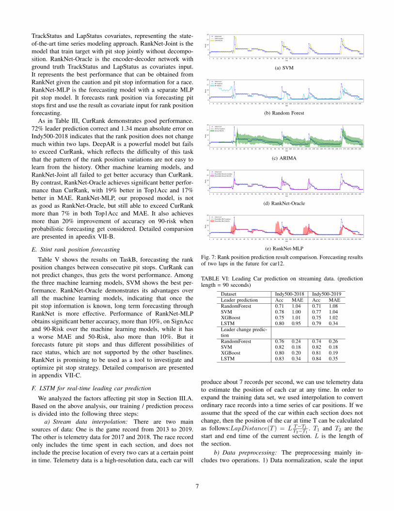
TrackStatus and LapStatus covariates, representing the state-of-the-art time series modeling approach. RankNet-Joint is themodel that train target with pit stop jointly without decompo-sition. RankNet-Oracle is the encoder-decoder network withground truth TrackStatus and LapStatus as covariates input.It represents the best performance that can be obtained fromRankNet given the caution and pit stop information for a race.RankNet-MLP is the forecasting model with a separate MLPpit stop model. It forecasts rank position via forecasting pitstops first and use the result as covariate input for rank positionforecasting.
As in Table III, CurRank demonstrates good performance.72% leader prediction correct and 1.34 mean absolute error onIndy500-2018 indicates that the rank position does not changemuch within two laps. DeepAR is a powerful model but failsto exceed CurRank, which reflects the difficulty of this taskthat the pattern of the rank position variations are not easy tolearn from the history. Other machine learning models, andRankNet-Joint all failed to get better accuracy than CurRank.By contrast, RankNet-Oracle achieves significant better perfor-mance than CurRank, with 19% better in Top1Acc and 17%better in MAE. RankNet-MLP, our proposed model, is notas good as RankNet-Oracle, but still able to exceed CurRankmore than 7% in both Top1Acc and MAE. It also achievesmore than 20% improvement of accuracy on 90-risk whenprobabilistic forecasting get considered. Detailed comparsionare presented in apeedix VII-B.
E. Stint rank position forecasting
Table V shows the results on TaskB, forecasting the rankposition changes between consecutive pit stops. CurRank cannot predict changes, thus gets the worst performance. Amongthe three machine learning models, SVM shows the best per-formance. RankNet-Oracle demonstrates its advantages overall the machine learning models, indicating that once thepit stop information is known, long term forecasting throughRankNet is more effective. Performance of RankNet-MLPobtains significant better accuracy, more than 10%, on SignAccand 90-Risk over the machine learning models, while it hasa worse MAE and 50-Risk, also more than 10%. But itforecasts future pit stops and thus different possibilities ofrace status, which are not supported by the other baselines.RankNet is promising to be used as a tool to investigate andoptimize pit stop strategy. Detailed comparison are presentedin appendix VII-C.
F. LSTM for real-time leading car prediction
We analyzed the factors affecting pit stop in Section III.A.Based on the above analysis, our training / prediction processis divided into the following three steps:
a) Stream data interpolation: There are two mainsources of data: One is the game record from 2013 to 2019.The other is telemetry data for 2017 and 2018. The race recordonly includes the time spent in each section, and does notinclude the precise location of every two cars at a certain pointin time. Telemetry data is a high-resolution data, each car will
1 6 11 16 21 26 31 36 41 46 51 56 61 66 71 76 81 86 91 96 101 106 111 116 121 126 131 136 141 146 151 156 161 166 171 176 181 186 191 196Lap
0
5
10
15
20
Rank
observedSVR-medianSVR-90.0%
(a) SVM
1 6 11 16 21 26 31 36 41 46 51 56 61 66 71 76 81 86 91 96 101 106 111 116 121 126 131 136 141 146 151 156 161 166 171 176 181 186 191 196Lap
0
5
10
15
20
Rank
observedRF-medianRF-90.0%
(b) Random Forest
1 6 11 16 21 26 31 36 41 46 51 56 61 66 71 76 81 86 91 96 101 106 111 116 121 126 131 136 141 146 151 156 161 166 171 176 181 186 191 196Lap
0
5
10
15
20
Rank
observedArima-medianArima-90.0%
(c) ARIMA
1 6 11 16 21 26 31 36 41 46 51 56 61 66 71 76 81 86 91 96 101 106 111 116 121 126 131 136 141 146 151 156 161 166 171 176 181 186 191 196Lap
0
5
10
15
20
Rank
observedRrankNet-Oracle-medianRrankNet-Oracle-90.0%
(d) RankNet-Oracle
1 6 11 16 21 26 31 36 41 46 51 56 61 66 71 76 81 86 91 96 101 106 111 116 121 126 131 136 141 146 151 156 161 166 171 176 181 186 191 196Lap
0
5
10
15
20
Rank
observedRrankNet-MLP-medianRrankNet-MLP-90.0%
(e) RankNet-MLP
Fig. 7: Rank position prediction result comparison. Forecasting resultsof two laps in the future for car12.
TABLE VI: Leading Car prediction on streaming data. (predictionlength = 90 seconds)
Dataset Indy500-2018 Indy500-2019Leader prediction Acc MAE Acc MAERandomForest 0.71 1.04 0.71 1.08SVM 0.78 1.00 0.77 1.04XGBoost 0.75 1.01 0.75 1.02LSTM 0.80 0.95 0.79 0.34Leader change predic-tionRandomForest 0.76 0.24 0.74 0.26SVM 0.82 0.18 0.82 0.18XGBoost 0.80 0.20 0.81 0.19LSTM 0.83 0.34 0.84 0.35
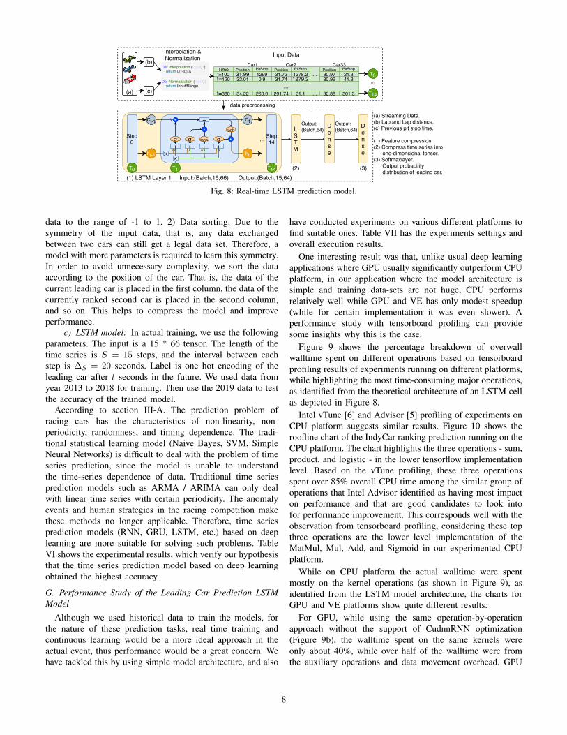
produce about 7 records per second, we can use telemetry datato estimate the position of each car at any time. In order toexpand the training data set, we used interpolation to convertordinary race records into a time series of car positions. If weassume that the speed of the car within each section does notchange, then the position of the car at time T can be calculatedas follows:LapDistance(T ) = L T−T1
T2−T1. T1 and T2 are the
start and end time of the current section. L is the length ofthe section.
b) Data preprocessing: The preprocessing mainly in-cludes two operations. 1) Data normalization, scale the input
7
Position PitStop31.99 1299
Position PitStop31.72 1278.2
Position PitStop30.97 21.3
Timet=100t=120 32.01 0.9 31.74 1279.2
...30.99 41.3
...
Def Interpolation (Input, t): return L(t-t0)/Δ
Def Normalization (Input): return Input/Range
Car33Car2Car1
+ + + +
• +•
•
ht-1
T1
Ct-1
ht
Ct
σ σ σtanh
tanh
✕✕
Interpolation &Normalization Input Data
Step0
Step14
T14T0
...
(1) LSTM Layer 1
LSTM
Dense
Dense
Input:(Batch,15,66) Output:(Batch,15,64)
data preprocessing
(b)
(c)
(a) Streaming Data.(b) Lap and Lap distance.(c) Previous pit stop time.
(1) Feature compression.(2) Compress time series into one-dimensional tensor.(3) Softmaxlayer. Output probability distribution of leading car.
...(a)
T0...
T14
(2) (3)
Output:(Batch,64)
Output:(Batch,64)
t=380 34.22 260.9 291.74 21.1 32.88 301.3...
Fig. 8: Real-time LSTM prediction model.
data to the range of -1 to 1. 2) Data sorting. Due to thesymmetry of the input data, that is, any data exchangedbetween two cars can still get a legal data set. Therefore, amodel with more parameters is required to learn this symmetry.In order to avoid unnecessary complexity, we sort the dataaccording to the position of the car. That is, the data of thecurrent leading car is placed in the first column, the data of thecurrently ranked second car is placed in the second column,and so on. This helps to compress the model and improveperformance.
c) LSTM model: In actual training, we use the followingparameters. The input is a 15 * 66 tensor. The length of thetime series is S = 15 steps, and the interval between eachstep is ∆S = 20 seconds. Label is one hot encoding of theleading car after t seconds in the future. We used data fromyear 2013 to 2018 for training. Then use the 2019 data to testthe accuracy of the trained model.
According to section III-A. The prediction problem ofracing cars has the characteristics of non-linearity, non-periodicity, randomness, and timing dependence. The tradi-tional statistical learning model (Naive Bayes, SVM, SimpleNeural Networks) is difficult to deal with the problem of timeseries prediction, since the model is unable to understandthe time-series dependence of data. Traditional time seriesprediction models such as ARMA / ARIMA can only dealwith linear time series with certain periodicity. The anomalyevents and human strategies in the racing competition makethese methods no longer applicable. Therefore, time seriesprediction models (RNN, GRU, LSTM, etc.) based on deeplearning are more suitable for solving such problems. TableVI shows the experimental results, which verify our hypothesisthat the time series prediction model based on deep learningobtained the highest accuracy.
G. Performance Study of the Leading Car Prediction LSTMModel
Although we used historical data to train the models, forthe nature of these prediction tasks, real time training andcontinuous learning would be a more ideal approach in theactual event, thus performance would be a great concern. Wehave tackled this by using simple model architecture, and also
have conducted experiments on various different platforms tofind suitable ones. Table VII has the experiments settings andoverall execution results.
One interesting result was that, unlike usual deep learningapplications where GPU usually significantly outperform CPUplatform, in our application where the model architecture issimple and training data-sets are not huge, CPU performsrelatively well while GPU and VE has only modest speedup(while for certain implementation it was even slower). Aperformance study with tensorboard profiling can providesome insights why this is the case.
Figure 9 shows the percentage breakdown of overwallwalltime spent on different operations based on tensorboardprofiling results of experiments running on different platforms,while highlighting the most time-consuming major operations,as identified from the theoretical architecture of an LSTM cellas depicted in Figure 8.
Intel vTune [6] and Advisor [5] profiling of experiments onCPU platform suggests similar results. Figure 10 shows theroofline chart of the IndyCar ranking prediction running on theCPU platform. The chart highlights the three operations - sum,product, and logistic - in the lower tensorflow implementationlevel. Based on the vTune profiling, these three operationsspent over 85% overall CPU time among the similar group ofoperations that Intel Advisor identified as having most impacton performance and that are good candidates to look intofor performance improvement. This corresponds well with theobservation from tensorboard profiling, considering these topthree operations are the lower level implementation of theMatMul, Mul, Add, and Sigmoid in our experimented CPUplatform.
While on CPU platform the actual walltime were spentmostly on the kernel operations (as shown in Figure 9), asidentified from the LSTM model architecture, the charts forGPU and VE platforms show quite different results.
For GPU, while using the same operation-by-operationapproach without the support of CudnnRNN optimization(Figure 9b), the walltime spent on the same kernels wereonly about 40%, while over half of the walltime were fromthe auxiliary operations and data movement overhead. GPU
8

TABLE VII: Experiments Hardware Specification and Overall Performance of the Leading Car Prediction LSTM Model Running on DifferentPlatforms. The model was implemented as a tensorflow keras model. CPU and GPU experiments used the official v2.0 tensorflow, whileVector Engine (VE) used a experimental forked version from the same version [10]. The cpu-only results were using only CPU resourceson each specified platform. The results were training speed (µs/sample). The speed up showed the results with accelerator compared to thecpu-only results for that platform. For GPU platform, one result was with CudnnRNN support and the other one without.
Platform CPU with speedup Hardwareonly Accelerator Specification
CPU 268 Intel Xeon E5-2670 [email protected], with 128G RAM
CPU+GPU 299 397 0.75 Intel Xeon CPU E5-2630 v4,244 (with 1.22 with 128G RAM;CudnnRNN) GPU (V100-SXM2-16GB)
CPU+VE 262 223 1.17 Intel Xeon Gold 6126 [email protected], with 192G RAM;VE (SX-Aurora Vector Engine)
CPU GPU VE
Mat
Mul
Mul
Sig
moi
d+Ta
nh+
Add
The
res
t
0
10
20
30
40
50
CPU
Ope
ratio
n W
allti
me
(%)
(a) CPU
Dat
a
Dat
a
Res
t
Res
t
Add
Add
, Sig
moi
d, T
anh
Mat
Mul
, Mul
Mat
Mul
, Mul
0
10
20
30
CPU/GPU
Ope
ratio
n W
allti
me
(%)
(b) CPU/GPU
Dat
a
Dat
a
Res
t
Res
t
Add
, Sig
moi
d, T
anh
AddMat
Mul
, Mul
Mat
Mul
, Mul
0
10
20
CPU/VE
Ope
ratio
n W
allti
me
(%)
(c) CPU/VE
Dat
a
Dat
a
Res
t
Res
t
Add
Add
, Sig
moi
d, T
anh
Cud
nnR
NN
Ops
Mat
Mul
, Mul
Mat
Mul
, Mul
0
10
20
30
40
CPU/GPU with CudnnRNN Core Enabled
Ope
ratio
n W
allti
me
(%)
(d) CPU/GPU with CudnnRNN
Fig. 9: Operation Walltime Percentage on Different Platforms. On CPU platform (a), the kernel operations (MatMul, Mul, Add, Sigmoid,Tanh) accounts for over 75% of the overall walltime spent. On GPU platform (b), 2/3 walltime were spent on the accelerator side but only40% were spent on the kernels and 25% were on other auxiliary operations. On VE platform (c) about 80% walltime spent on CPU sidewhile the rest were offloaded to VE side. On GPU platform with CudnnRNN support (d), due to the CudnnRNN optimization the majoroperations were not the same kernel operations.
0.01 0.05 0.50 5.00
15
5050
0
FLOP/Byte (Arithmetic Intensity)
GF
LOP
S
DRAM
L3
Scalar Add Peak
DP Vector FMA Peaksum (used by MatMul, Add)product (used by MatMul, Mul)logistic (used by Sigmoid)
sumproductlogistic
Fig. 10: Roofline chart of the IndyCar Ranking Prediction ModelRunning on the CPU Platform. The chart hightlights the operationsin the lower tensorflow implementation level of the identified kernels- MatMul, Mul, Add, and Sigmoid.
with CudnnRNN optimization (Figure 9d) has improved thissituation by minimizing the overhead and fully utilizing thehardware advantage of GPU. This optimization for LSTM andRNN models in CUDA library [8], [14] includes combining
and streaming matrix multiplication operations to improve theparallelism as well as fusing point-wise operations to reducedata movement overhead and kernel invocation overhead,among other tricks for more complex model. The result was afaster execution time with a 1.22x speedup, comparing to theoperation-by-operation approach which was actually slowerthan the CPU-only approach.
Vector Engine on NEC SX-Aurora machine provides an-other possible good fit due to its high memory bandwidth andhigh efficiency for vectorized operations. Figure 9c shows thesame operation percentage breakdown and allocation betweenVector Host (CPU) and VE. Among the kernel operations,Sigmoid and Tanh were all offloaded to the VE side, while forMatMul, Mul, and Add the operations occurred on both side.The offloading strategy of certain operations from VH to VEwas based on the criteria that the potential walltime saved canoffset the overhead from offloading, so the small insignificantcalculations would be just handled on CPU side. Still, theoverhead from auxiliary operations and data movement wasquite significant. If similar fusing operation strategy were to
9

applied, this large portion of the overhead could be potentiallyminimized thus achieving higher speedup.
In either GPU or VE case, for more complex model andlarger data we expect the benefit from operation offload-ing from CPU to accelerator would largely exceed the datamovement and kernel launch overhead thus obtaining higherspeedup. We have observed this during the iteration of modeloptimization, when we experimented on one previous similarbut more complex model, in which we observed about 2xspeedup for both GPU and VE.
V. RELATED WORK
Forecasting in general: Forecasting is a heavily studiedproblem interested across domains. decomposition to addressuncertainty. Classical statistical methods(e.g,ARIMA and ex-ponential smoothing) and machine learning methods(e.g, SVR,Random Forest and XGB) are wildly applied in the problemswith few of randomness, non-stationary and irregularity. Todeal with the problem of high uncertainty, decomposition andensemble is often used to separate the uncertainty signalsfrom the normal patterns and model them in dependently. [26]utilizes the Empirical Mode Decomposition [22] algorithm todecompose the load demand data into several intrinsic modefunctions and one residue, then models each of them separatelyby a deep belief network, finally forecast by the ensembleof the sub-models. Another type of decomposition occursin local and global modeling. ES-RNN [31], winner of M4forecasting competition [7], hybrids exponential smoothing tocapture non-stationary trends per series and learn global effectsby RNN, ensemble the outputs finally. Similar approaches areadopted in DeepState [27], DeepFactor [35]. In this work,based on the understanding of the cause effects of the problem,we decompose the uncertainty by modeling the causal factorsand the target series separately and hybrid the sub-modelsaccording to the cause effects relationship. Different fromthe works of counterfactual prediction [12], [19], we do notdiscover causal effects from data.
modeling extreme events. Extreme events [23] are featuredwith rare occurrence, difficult to model, and their predictionare of a probabilistic nature. [24], [36] use a autoencoder tocapture complex time-series dynamics during extreme events,show improved results. Autoencoder shows improve resultsin capturing complex time-series dynamics during extremeevents, such as [24] for uber riding forecasting and [36] whichdecomposes normal traffic and accidents for traffic forecasting.[17] proposes to use a memory network with attention tocapture the extreme events pattern and a novel loss functionbased on extreme value theory. In our work, we classifythe extreme events in car racing into different categories,model the more preditable pit stops in normal laps by MLPwith probabilistic output. Exploring autoencoder and memorynetwork can be one of our future work.
express uncertainty in model. [18] first proposed to modeluncertainty in deep neural network by using dropout as aBayesian approximation. [36] followed this idea and success-fully apply it to large-scale time series anomaly detection at
Uber. Our work follows the idea in [29] that parameterizesa fixed distribution with the output of a neural network. [34]adopts the same idea and apply it to weather forecasting.
Car racing forecasting: Simulation-based method:Racingsimulation is widely used in motor sports analysis [1], [15],[20]. To calculating the final race time for all the carsaccurately, a racing simulator models different factors thatimpact lap time during the race, such as car interactions, tyredegradation, fuel consumption, pit stop etc., via equationswith fine tuned parameters. Specific domain knowledge arenecessary to build successful simulation models. [20] presentsa simulator that reduce the race time calculation error toaround one second for Formula 1 2017 Abu Dhabi Grand Prix.But, the author mentioned that user is required to provide thepit stop information for every driver as an input.
Machine learning-based method: [16], [32] is a series ofwork forecasting the decision-to-decision loss in rank posi-tion for each racer in NASCAR. [32] describes how theyleveraged expert knowledge of the domain to produce a real-time decision system for tire changes within a NASCAR race.They chose to model the change in rank position and avoidpredicting the rank position directly since it is complicateddue to its dependency on the timing of other racers’ pit stops.In our work, we aim to build a forecasting that rely less ondomain knowledge and investigate the pit stop modeling.
VI. CONCLUSION
In this work, we build rank position forecasting model forcar racing on IndyCar dataset. We adopt the deep learningmodeling approach that aims to do it best to automaticallyextract features and learn effective model, reducing the de-pendency on domain experts in other machine learning andsimulation approaches. A combination of encoder-decodernetwork and separate MLP network that capable to deliverprobabilistic forecasting are proposed to model the pit stopevents and rank position in car racing.
Through extensive evaluation experiments, we find thatpit stop information is critical for rank position forecastingtasks. Our proposed model achieves significant better accuracythan baseline models when pit stop information are given.When using predicted pit stop information, the model obtainscomparable performance in both the rank position forecastingtask and change of the rank position forecasting task, withthe advantages of needing less feature engineering efforts andproviding probabilistic forecasting that enables racing strategyoptimizations via our deep learning based model.
There are several limitations of this work. Since there arenot many related work, the performance evaluation in thispaper is still limited. An other major challenge lies in thelimitation of the volume of the dataset. Car racing is a one timeevent that the observed data are always limited. Consideringto add extra information with finer granularity could be onedirection of our future work.
REFERENCES
[1] Building a Race Simulator. https://f1metrics.wordpress.com/2014/10/03/building-a-race-simulator/. visited on 04/15/2020.
10
[2] IndyCar Dataset. https://racetools.com/logfiles/IndyCar/. visited on04/15/2020.
[3] IndyCar Stats. https://www.indycar.com/Stats.[4] IndyCar Understanding-The-Sport. https://www.indycar.com/Fan-
Info/INDYCAR-101/Understanding-The-Sport/Timing-and-Scoring.visited on 04/15/2020.
[5] Intel Advisor. https://software.intel.com/content/www/us/en/develop/tools/advisor.html.[6] Intel vTune. https://software.intel.com/content/www/us/en/develop/tools/vtune-
profiler.html.[7] M4Competition. https://forecasters.org/resources/timeseriesdata/m4-
competition/. visited on 04/15/2020.[8] Optimizing Recurrent Neural Networks in cuDNN 5.
https://devblogs.nvidia.com/optimizing-recurrent-neural-networks-cudnn-5/.
[9] PitStop. https://en.wikipedia.org/wiki/Pit stop. visited on 04/15/2020.[10] TensorFlow for SX-Aurora TSUBASA. https://github.com/sx-aurora-
dev/tensorflow.[11] B. Adhikari, X. Xu, N. Ramakrishnan, and B. A. Prakash. EpiDeep:
Exploiting Embeddings for Epidemic Forecasting. In Proceedings of the25th ACM SIGKDD International Conference on Knowledge Discovery& Data Mining, KDD ’19, pages 577–586, New York, NY, USA, 2019.ACM. event-place: Anchorage, AK, USA.
[12] A. M. Alaa, M. Weisz, and M. van der Schaar. Deep CounterfactualNetworks with Propensity-Dropout. arXiv:1706.05966 [cs, stat], June2017. arXiv: 1706.05966.
[13] A. Alexandrov, K. Benidis, M. Bohlke-Schneider, V. Flunkert,J. Gasthaus, T. Januschowski, D. C. Maddix, S. Rangapuram, D. Salinas,J. Schulz, L. Stella, A. C. Turkmen, and Y. Wang. GluonTS: Proba-bilistic Time Series Models in Python. arXiv:1906.05264 [cs, stat], June2019. arXiv: 1906.05264.
[14] J. Appleyard, T. Kocisky, and P. Blunsom. Optimizing performance ofrecurrent neural networks on gpus. arXiv preprint arXiv:1604.01946,2016.
[15] J. Bekker and W. Lotz. Planning Formula One race strategies usingdiscrete-event simulation. Journal of the Operational Research Society,60(7):952–961, 2009. Publisher: Taylor & Francis.
[16] C. L. W. Choo. Real-time decision making in motorsports: analytics forimproving professional car race strategy. PhD Thesis, MassachusettsInstitute of Technology, 2015.
[17] D. Ding, M. Zhang, X. Pan, M. Yang, and X. He. Modeling ExtremeEvents in Time Series Prediction. In Proceedings of the 25th ACMSIGKDD International Conference on Knowledge Discovery & DataMining, KDD ’19, pages 1114–1122, New York, NY, USA, 2019. ACM.event-place: Anchorage, AK, USA.
[18] Y. Gal and Z. Ghahramani. Dropout as a bayesian approximation:Representing model uncertainty in deep learning. In internationalconference on machine learning, pages 1050–1059, 2016.
[19] J. Hartford, G. Lewis, K. Leyton-Brown, and M. Taddy. Deep IV:a flexible approach for counterfactual prediction. In Proceedings ofthe 34th International Conference on Machine Learning - Volume70, ICML’17, pages 1414–1423, Sydney, NSW, Australia, Aug. 2017.JMLR.org.
[20] A. Heilmeier, M. Graf, and M. Lienkamp. A Race Simulation forStrategy Decisions in Circuit Motorsports. In 2018 21st InternationalConference on Intelligent Transportation Systems (ITSC), pages 2986–2993, Nov. 2018.
[21] A. Heilmeier, M. Graf, and M. Lienkamp. A race simulation for strategydecisions in circuit motorsports. In 2018 21st International Conferenceon Intelligent Transportation Systems (ITSC), pages 2986–2993. IEEE,2018.
[22] N. E. Huang, Z. Shen, S. R. Long, M. C. Wu, H. H. Shih, Q. Zheng, N.-C. Yen, C. C. Tung, and H. H. Liu. The empirical mode decompositionand the Hilbert spectrum for nonlinear and non-stationary time seriesanalysis. Proceedings of the Royal Society of London. Series A:mathematical, physical and engineering sciences, 454(1971):903–995,1998. Publisher: The Royal Society.
[23] H. Kantz, E. G. Altmann, S. Hallerberg, D. Holstein, and A. Riegert.Dynamical Interpretation of Extreme Events: Predictability and Predic-tions. In S. Albeverio, V. Jentsch, and H. Kantz, editors, Extreme Eventsin Nature and Society, The Frontiers Collection, pages 69–93. Springer,Berlin, Heidelberg, 2006.
[24] N. Laptev, J. Yosinski, L. E. Li, and S. Smyl. Time-series extreme eventforecasting with neural networks at uber. In International Conferenceon Machine Learning, volume 34, pages 1–5, 2017.
[25] B. Liao, J. Zhang, C. Wu, D. McIlwraith, T. Chen, S. Yang, Y. Guo, andF. Wu. Deep Sequence Learning with Auxiliary Information for TrafficPrediction. In Proceedings of the 24th ACM SIGKDD InternationalConference on Knowledge Discovery & Data Mining, KDD ’18, pages537–546, New York, NY, USA, 2018. ACM. event-place: London,United Kingdom.
[26] X. Qiu, Y. Ren, P. N. Suganthan, and G. A. J. Amaratunga. EmpiricalMode Decomposition based ensemble deep learning for load demandtime series forecasting. Applied Soft Computing, 54:246–255, May 2017.
[27] S. S. Rangapuram, M. W. Seeger, J. Gasthaus, L. Stella, Y. Wang, andT. Januschowski. Deep state space models for time series forecasting. InAdvances in neural information processing systems, pages 7785–7794,2018.
[28] R. Ryan, H. Zhao, and M. Shao. CTC-Attention based Non-ParametricInference Modeling for Clinical State Progression. In 2019 IEEEInternational Conference on Big Data (Big Data), pages 145–154, Dec.2019.
[29] D. Salinas, V. Flunkert, J. Gasthaus, and T. Januschowski. DeepAR:Probabilistic forecasting with autoregressive recurrent networks. Inter-national Journal of Forecasting, Oct. 2019.
[30] M. W. Seeger, D. Salinas, and V. Flunkert. Bayesian intermittent demandforecasting for large inventories. In Advances in Neural InformationProcessing Systems, pages 4646–4654, 2016.
[31] S. Smyl. A hybrid method of exponential smoothing and recurrentneural networks for time series forecasting. International Journal ofForecasting, 36(1):75–85, Jan. 2020.
[32] T. Tulabandhula. Interactions between learning and decision making.PhD Thesis, Massachusetts Institute of Technology, 2014.
[33] T. Tulabandhula and C. Rudin. Tire changes, fresh air, and yellowflags: challenges in predictive analytics for professional racing. Bigdata, 2(2):97–112, 2014.
[34] B. Wang, J. Lu, Z. Yan, H. Luo, T. Li, Y. Zheng, and G. Zhang. Deepuncertainty quantification: A machine learning approach for weatherforecasting. In Proceedings of the 25th ACM SIGKDD InternationalConference on Knowledge Discovery & Data Mining, pages 2087–2095,2019.
[35] Y. Wang, A. Smola, D. C. Maddix, J. Gasthaus, D. Foster, andT. Januschowski. Deep Factors for Forecasting. arXiv:1905.12417 [cs,stat], May 2019. arXiv: 1905.12417.
[36] R. Yu, Y. Li, C. Shahabi, U. Demiryurek, and Y. Liu. Deep learning: Ageneric approach for extreme condition traffic forecasting. In Proceed-ings of the 2017 SIAM international Conference on Data Mining, pages777–785. SIAM, 2017.
VII. APPENDIX
A. Feature engineering and parameter tuning for machinelearning baselines
Three machine learning models, RandomForest, SVM and XG-Boost, have been presented as baselines in the forecasting tasks.
First, performance of machine learning models rely heavily onfeature engineering, e.g., [33] employs more than one hundred offeatures by the help of domain experts. In this work, we followthe similar ideas of feature extraction for the machine learningbaselines in the following five aspects: global information, Rank,LapTime, PitStop and features of the near neighbors, as in Table. VIII.RankNet, as a deep learning based forecasting model, demonstratesits advantages over traditional machine learning methods in the lowcost of feature engineering, as the recurrent neural network learnsbetter feature representations from the input sequence than manualfeature extractions deployed in Table. VIII.
Hyper-parameter tuning is another important factor for these ma-chine learning models. We deployed grid search and cross validationto find the optimal hyper parameters. In contrast, RankNet has lesshyper parameters.
B. Short-term rank position forecastingFig.11 demonstrate the performance improvement over a strong
baseline CurRank for all the models. It shows that the threemachine learning models, deep learning model DeepAR and thejoint train model RankNet-Joint all failed to get better accuracy than
11

TABLE VIII: Features extracted for machine learning models. In short-term forecasting, a stage is defined as a window with length of thesame context length in RankNet. In stint forecasting, a stage is the laps between two consecutive pit stops.
Type Feature Meaning
Gobal infostart position #rank at the beginning of the racestageid sequence id of stagefirststage is the first stage?
Rank
start rank #rank at the forecasting positionstart rank ratio #rank/totalcarnumtop pack #rank in top5?bottom pack #rank in bottom5?average rank
1st to 3rd moment of rank inprevious stagechange in rankrate of changeaverage rank all
1st to 3rd moment of rank inall previous stageschange in rank allrate of change all
Laptime
laptime green mean prev mean and std of the lap time in green laps of the previous stagelaptime green std prevlaptime green mean all mean and std of the lap time in all green laps beforelaptime green std alllaptime mean prev mean and std of the lap time in all laps of the previous stagelaptime std prevlaptime mean all mean and std of the lap time in all laps beforelaptime std all
Pitstop
pit in caution the previous pit in caution laplaps prev lap number to the previous pitstopcautionlaps prev caution laps number to the previous pitstoppittime prev pit time of the previous pitstop
Neighbors’ Info nb change in rank features of three previous cars and three following carsnb laptime difference
-0.07
-0.29
0.00
-0.36
0.01
0.19
0.07
-0.54
-0.31
0.00
-0.22-0.30
0.17
0.07
-0.61
-0.31
-0.01
-0.23
-0.45
0.180.11
0.01
-0.31
-0.01
-0.23
0.11
0.240.20
Per
form
ance
Impr
ovem
ent
-0.75
-0.50
-0.25
0.00
0.25
DeepA
R
Rando
mForest
SVM
XGBoost
RankN
et-Jo
int
RankN
et-Orac
le
RankN
et-MLP
DeepA
R
Rando
mForest
SVM
XGBoost
RankN
et-Jo
int
RankN
et-Orac
le
RankN
et-MLP
DeepA
R
Rando
mForest
SVM
XGBoost
RankN
et-Jo
int
RankN
et-Orac
le
RankN
et-MLP
DeepA
R
Rando
mForest
SVM
XGBoost
RankN
et-Jo
int
RankN
et-Orac
le
RankN
et-MLP
Top1Acc MAE 50-Risk 90-Risk
Performance Improvement over CurRank
Fig. 11: Performance comparison for short-term forecasting modelson Indy500-2018.
CurRank. By contrast, RankNet-Oracle achieves significant betterperformance than CurRank, with 19% better in Top1Acc and 17%better in MAE. RankNet-MLP, our proposed model, is not as goodas RankNet-Oracle, but still able to exceed CurRank more than7% in both Top1Acc and MAE. It also achieves more than 20%improvement of accuracy on 90-risk when probabilistic forecastingget considered.
C. Stint rank position forecastingFor long-term forecasting, CurRank does not perform well.
Fig.12(a) demonstrate the performance improvement over a baselineSVM for all the models. Performance of RankNet-MLP obtainssignificant better accuracy, more than 10%, on SignAcc and 90-Riskover the machine learning models, while it has a worse MAE and50-Risk, also more than 10%.
Fig.12(b) shows an example of stint forecasting with 100 samplesat pit stop lap 94 for car 12 in Indy500-2018. When the observed
-0.05
-0.19
0.180.13
-0.04
-0.20
0.04
-0.12
-0.04
-0.20
0.03
-0.12
-0.04
-0.10
0.11
0.23
Per
form
ance
Impr
ovem
ent
-0.30
-0.20
-0.10
0.00
0.10
0.20
0.30
Rando
mForest
XGBoost
RankN
et-Orac
le
RankN
et-MLP
Rando
mForest
XGBoost
RankN
et-Orac
le
RankN
et-MLP
Rando
mForest
XGBoost
RankN
et-Orac
le
RankN
et-MLP
Rando
mForest
XGBoost
RankN
et-Orac
le
RankN
et-MLP
SignAcc MAE 50-Risk 90-Risk
Performance Improvement over SVM
113 114 115 116 117 118 119 120 121 122 123 124 125 126 127 128 129Predicted Lap of Next PitStop
0.0
2.5
5.0
7.5
10.0
12.5
15.0
Prob
abilit
y(%
)
0 1 2 3 4 5 6 7 8Predicted Rank Posisiton of Next PitStop
0
20
40
60
80
Prob
abilit
y(%
)
observedforecast
Fig. 12: Performance comparison for stint forecasting models onIndy500-2018.
next pit stop lap is 128, RankNet-MLP predicts it with probabilityaround 3%. Accordingly, observed rank at next pit stop is 1, andRankNet-MLP predicts it with probability 22%. This deviationcomes from the uncertainty of extreme events and the bias of thetrained model. Because of the sparsity of data, the PitModel istrained on data from 2013 to 2017, improvements of the cars enablethem run longer between pit stops at 2018, which may bring bias.
D. Impact of Oracle FeaturesAn oracle model, a model given the future pit stop information as
input, can be used to represents the upper bound of performance that
12
-0.17
-0.08
-0.23
-0.02 -0.03
-0.09
-0.01 -0.03
-0.08-0.11
-0.55
-0.06
Per
form
ance
Impr
ovem
ent o
ver R
ankN
et
-0.60
-0.40
-0.20
0.00
Rando
mForest
SVM
XGBoost
Rando
mForest
SVM
XGBoost
Rando
mForest
SVM
XGBoost
Rando
mForest
SVM
XGBoost
SignAcc MAE 50-Risk 90-Risk
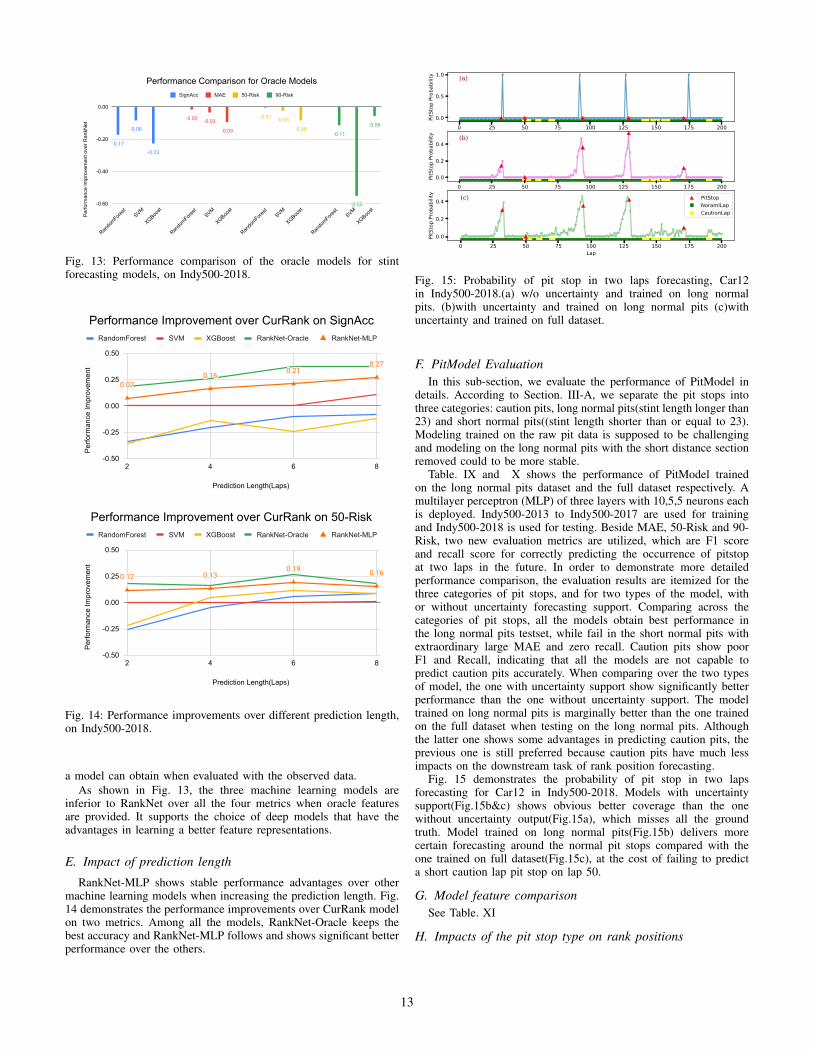
Performance Comparison for Oracle Models
Fig. 13: Performance comparison of the oracle models for stintforecasting models, on Indy500-2018.
0.070.16
0.210.27
Prediction Length(Laps)
Per
form
ance
Impr
ovem
ent
-0.50
-0.25
0.00
0.25
0.50
2 4 6 8
RandomForest SVM XGBoost RankNet-Oracle RankNet-MLP
Performance Improvement over CurRank on SignAcc
0.12 0.130.19 0.16
Prediction Length(Laps)
Per
form
ance
Impr
ovem
ent
-0.50
-0.25
0.00
0.25
0.50
2 4 6 8
RandomForest SVM XGBoost RankNet-Oracle RankNet-MLP
Performance Improvement over CurRank on 50-Risk
Fig. 14: Performance improvements over different prediction length,on Indy500-2018.
a model can obtain when evaluated with the observed data.As shown in Fig. 13, the three machine learning models are
inferior to RankNet over all the four metrics when oracle featuresare provided. It supports the choice of deep models that have theadvantages in learning a better feature representations.
E. Impact of prediction length
RankNet-MLP shows stable performance advantages over othermachine learning models when increasing the prediction length. Fig.14 demonstrates the performance improvements over CurRank modelon two metrics. Among all the models, RankNet-Oracle keeps thebest accuracy and RankNet-MLP follows and shows significant betterperformance over the others.
0 25 50 75 100 125 150 175 200Lap
0.0
0.5
1.0
PitS
top
Prob
abilit
y (a)
0 25 50 75 100 125 150 175 200Lap
0.0
0.2
0.4
PitS
top
Prob
abilit
y (b)
0 25 50 75 100 125 150 175 200Lap
0.0
0.2
0.4
PitS
top
Prob
abilit
y
(c) PitStopNoramlLapCautionLap
Fig. 15: Probability of pit stop in two laps forecasting, Car12in Indy500-2018.(a) w/o uncertainty and trained on long normalpits. (b)with uncertainty and trained on long normal pits (c)withuncertainty and trained on full dataset.
F. PitModel EvaluationIn this sub-section, we evaluate the performance of PitModel in
details. According to Section. III-A, we separate the pit stops intothree categories: caution pits, long normal pits(stint length longer than23) and short normal pits((stint length shorter than or equal to 23).Modeling trained on the raw pit data is supposed to be challengingand modeling on the long normal pits with the short distance sectionremoved could to be more stable.
Table. IX and X shows the performance of PitModel trainedon the long normal pits dataset and the full dataset respectively. Amultilayer perceptron (MLP) of three layers with 10,5,5 neurons eachis deployed. Indy500-2013 to Indy500-2017 are used for trainingand Indy500-2018 is used for testing. Beside MAE, 50-Risk and 90-Risk, two new evaluation metrics are utilized, which are F1 scoreand recall score for correctly predicting the occurrence of pitstopat two laps in the future. In order to demonstrate more detailedperformance comparison, the evaluation results are itemized for thethree categories of pit stops, and for two types of the model, withor without uncertainty forecasting support. Comparing across thecategories of pit stops, all the models obtain best performance inthe long normal pits testset, while fail in the short normal pits withextraordinary large MAE and zero recall. Caution pits show poorF1 and Recall, indicating that all the models are not capable topredict caution pits accurately. When comparing over the two typesof model, the one with uncertainty support show significantly betterperformance than the one without uncertainty support. The modeltrained on long normal pits is marginally better than the one trainedon the full dataset when testing on the long normal pits. Althoughthe latter one shows some advantages in predicting caution pits, theprevious one is still preferred because caution pits have much lessimpacts on the downstream task of rank position forecasting.
Fig. 15 demonstrates the probability of pit stop in two lapsforecasting for Car12 in Indy500-2018. Models with uncertaintysupport(Fig.15b&c) shows obvious better coverage than the onewithout uncertainty output(Fig.15a), which misses all the groundtruth. Model trained on long normal pits(Fig.15b) delivers morecertain forecasting around the normal pit stops compared with theone trained on full dataset(Fig.15c), at the cost of failing to predicta short caution lap pit stop on lap 50.
G. Model feature comparisonSee Table. XI
H. Impacts of the pit stop type on rank positions
13
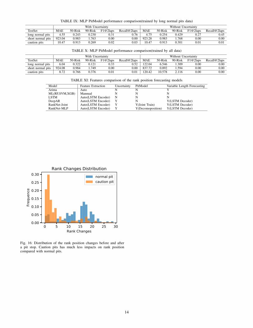
TABLE IX: MLP PitModel performance comparison(trained by long normal pits data)
With Uncertainty Without UncertaintyTestSet MAE 50-Risk 90-Risk F1@2laps Recall@2laps MAE 50-Risk 90-Risk F1@2laps Recall@2lapslong normal pits 4.55 0.243 0.230 0.31 0.76 4.75 0.254 0.429 0.27 0.45short normal pits 923.04 0.983 1.763 0.00 0.00 923.28 0.983 1.768 0.00 0.00caution pits 10.47 0.913 0.269 0.02 0.03 10.47 0.913 0.301 0.01 0.01
TABLE X: MLP PitModel performance comparison(trained by all data)
With Uncertainty Without UncertaintyTestSet MAE 50-Risk 90-Risk F1@2laps Recall@2laps MAE 50-Risk 90-Risk F1@2laps Recall@2lapslong normal pits 6.04 0.322 0.121 0.33 0.52 122.04 6.546 1.309 0.00 0.00short normal pits 924.08 0.984 1.749 0.00 0.00 837.72 0.892 1.594 0.00 0.00caution pits 8.72 0.766 0.376 0.01 0.01 120.42 10.578 2.116 0.00 0.00
TABLE XI: Features comparison of the rank position forecasting models
Model Feature Extraction Uncertainty PitModel Variable Length ForecastingArima Auto N N YML(RF,SVM,XGB) Mannual N N NLSTM Auto(LSTM Encoder) N N NDeepAR Auto(LSTM Encoder) Y N Y(LSTM Decoder)RankNet-Joint Auto(LSTM Encoder) Y Y(Joint Train) Y(LSTM Decoder)RankNet-MLP Auto(LSTM Encoder) Y Y(Decomoposition) Y(LSTM Decoder)
0 5 10 15 20 25 30Rank Changes
0.00
0.05
0.10
0.15
0.20
0.25
0.30
Freq
uenc
e
Rank Changes Distributionnormal pitcaution pit
Fig. 16: Distribution of the rank position changes before and aftera pit stop. Caution pits has much less impacts on rank positioncompared with normal pits.
14