arX

iv:0

810.

0394

v1 [

cs.P

F] 2

Oct

200

8

Mobility Management Framework

Peter Fulopa,∗, Benedek Kovacsb,∗, Sandor Imrec,∗,

a,cDepartment of Telecommunications, Budapest University of Technology H-1521

Pf. 91,Hungary,b Department of Mathematical Analysis, Budapest University of Technology

H-1111, 1 Egry Jozsef Hungary

Abstract

This paper investigates mobility management strategies from the point of view of

their need of signalling and processing resources on the backbone network and load on

the air interface. A method is proposed to model the serving network and mobile node

mobility in order to be able to compare the different types of mobility management

algorithms. To obtain a good description of the network we calculate descriptive

parameters from given topologies. Most mobility approaches derived from existing

protocols are analyzed and their performances are numerically compared in various

network and mobility scenarios. We developed a mobility management framework

that is able to give general designing guidelines for the next generation mobility

managements on given network, technology and mobility properties. With our model

an operator can design the network and tune the parameters to obtain the optimal

implementation of course revising existing systems is also possible. We present a

vertical handover decision method as a special application of our model framework.

Key words: mobility, management, modeling, network, graph

1 Introduction

Information mobility has became one of the most common services in the mod-ern world with the widespread of the portable phones and other mobile equip-ments. The wireless multimedia and other services has many requirements andthe resources in the serving network are often expensive and limited.

Email address: {fulopp,imre}@hit.bme.hu,bence@mcl.hu (Peter Fulopa,∗,Benedek Kovacsb,∗, Sandor Imrec,∗).

Preprint submitted to Elsevier 21 November 2021

We investigate mobility as an abstract problem regardless of actual technicalsolutions or serving network. In the first mobility protocol designs, the mainscope was to create a well-functioning mobility. For example, the Global Sys-tem for Mobile Communication (GSM) network uses a Cellular approach tosave bandwidth on the air interface but does not really focus on the problemof signalling load on the wired serving network. In the Mobile IP (MIP) [10]structure the IP mobility is in the main scope. There are many enhancementsof MIP to optimize the original protocol and introduces for example hierar-chy, location tracking to obtain a solution that is more cost efficient in a way.There are various other technologies, too. Host Identity Protocol (HIP) [5] isdrastically different from MIP although they have similar centralized mobil-ity approach but are implemented on a different network layer. The WirelessLocal Area Networks (WLAN) are constructed similarly to the original LocalArea Networks (LAN) and provide mobility only within the radio interface anduses Dynamic Host Configuration Protocol (DHCP). Future protocols mightuse different media and technological background to provide mobility.

The advantage in our work is that we do not focus on a selected technologynot even on a given network generation but discuss mobility in general withinthe modern computer and telecommunication networking technologies. To de-scribe the environment we focus on the bottlenecks such as the air interface,bandwidth on the core network and processing load on the network nodes andas one of the most significant properties: complexity involving scalability.

We compare selected mobility approaches and show how the network proper-ties affect the usability of each. The aim is to find the suitable one for differentscenarios and to give guidelines how to construct the network for a protocolor a protocol to the network. To generalize the model we have to uniformthe notations as well. The cooperating mobility management elements in ourapproach will be the Mobile Nodes (MNs) attaching to Mobility Access Points(MAPs) as a subset of the network of Mobility Agents (MAs).

This paper is structured as follows. The model for the network and the mobilenode with its mobility parameters are introduced in Section 3. This is followedwith the definitions of the cost functions for existing approaches in Section 4.One can see figures of the numerical results in Section 5 while the conclusionis derived in Section 6.

2 Mobility Management

In this paper the mobility management is discussed generally regardless of theparticular technology used. We try to grab the most significant properties ofthe mobility that is worth to discuss within the scope of the modern mobility

2

protocols.

2.1 The Mobility Management System

We define Mobility Management System – MMS as an application running onnetwork nodes that helps to locate the mobile equipment towards its uniqueidentifier (the IP address for example).

• The Mobile Nodes (MN) are the mobile equipments who want to commu-nicate to any other mobile or fixed partner.

• There are Mobility Access Points (MAP) as the only entities that directlyconnects the Mobile Equipments. (Note: mobility does not necessarily im-ply radio communication. It means only that the Mobile Node changes itsMobility Access Points and when it is attached to one, connection betweenthem can be established.)

• The Mobility Agents (MA) are network entities running the mobility man-agement application.

• There is a core network that provides communication between the MobilityAccess Points and has a structure that can be described with a graph.Vertices are either Mobility Access Points or Mobility Agents other servingnodes who are not part of the mobility management application and theedges can be various links (even radio links) for the data communicationbetween the vertices.

With this definition one can see that most of the functional entities of thecurrent mobility protocols and others under development can be generallydescribed. (Details and proof of the above statement is given in Section 4.)

We simplify the problem of mobility management to a protocol that finds thecorrect, marked Mobility Access Point where a given Mobile Node is attached.To create this model we need some practical assumptions:

• A Mobility Access Point is always a Mobility Agent.• All the nodes presented above are logical entities i.e. Mobility Access Pointscan mean a set of physical access points.

• A mobile equipment can communicate with multiple Access Points at thesame time but one connection is necessary and enough to maintain thecorrect communication. The mobile can also attach and detach from anyMobility Access Points. At this point we assume that the mobile node isadministrated only at one agent. This means that the problem of findingthe mobile node is the same as finding the correct access point. (It is notdifficult to enhance the discussion to the case where the MN can be find atmultiple MAPs but it is out of the scope of the paper.)

• The nodes in the core network communicate and find each other using a

3

given protocol or method (for example via IP routing). For this reason thispart of the mobility protocols is not discussed.

The above definition and assumptions suit our aim that is to investigate theproperties of various management strategy approaches, since the number ofmessages sent and the number of tasks should be completed can be calculated.With assigning appropriate cost parameters to each message or task one willbe able to model exact mobility management solutions and can analyze them.We are going to give an example in Section 5.

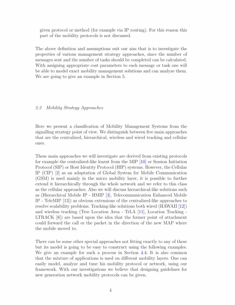
2.2 Mobility Strategy Approaches

Here we present a classification of Mobility Management Systems from thesignalling strategy point of view. We distinguish between five main approachesthat are the centralized, hierarchical, wireless and wired tracking and cellularones.

These main approaches we will investigate are derived from existing protocolsfor example the centralized-like learnt from the MIP [10] or Session InitiationProtocol (SIP) or Host Identity Protocol (HIP) systems. However, the CellularIP (CIP) [2] as an adaptation of Global System for Mobile Communication(GSM) is used mainly in the micro mobility layer, it is possible to furtherextend it hierarchically through the whole network and we refer to this classas the cellular approaches. Also we will discuss hierarchical-like solutions suchas (Hierarchical Mobile IP - HMIP [3], Telecommunication Enhanced MobileIP - TeleMIP [13]) as obvious extensions of the centralized-like approaches toresolve scalability problems. Tracking-like solutions both wired (HAWAII [12])and wireless tracking (Tree Location Area - TrLA [11], Location Tracking -LTRACK [8]) are based upon the idea that the former point of attachmentcould forward the call or the packet in the direction of the new MAP wherethe mobile moved to.

There can be some other special approaches not fitting exactly to any of thesebut its model is going to be easy to construct using the following examples.We give an example for such a process in Section 4.4. It is also commonthat the mixture of applications is used on different mobility layers. One caneasily model, analyze and tune his mobility protocol or network, using ourframework. With our investigations we believe that designing guidelines fornew generation network mobility protocols can be given.

4

3 Network Graph and Node Mobility Parameters

In this Section, we introduce how we will model the network structure on whichthe Mobility Management Systems work. To derive the main parameters wewill have to model the behavior of the Mobile Nodes as well. There will begeneral and algorithm specific parameters derived and also we will describehow we handle some protocol specific, extra problems like looping (how likelythat a mobile returns to a former MAP) and the frequency of location areachanges (how likely that a MN moves within a given subset of MAPs).

Secondly, we present the cost dimensions include to our model. These costparameters related to the “signalling on the links” as a bandwidth and inter-working equipment usage (or even QoS and Service Cost ratio), the “process-ing in the nodes” which are taken into account only on the nodes running themobility protocol, the “access cost” or “air interface usage” containing thecost of accessing the fixed network (MAP-MN attachment) or explicitly forexample the battery consumption of the MN.

3.1 Modelling the Network

As the first step we go through existing comparison works because in manypapers, the network is modelled in order to emphasize the properties of a sin-gle protocol compared to another one. This approach is not flexible since newprotocols cannot be imported to the comparison and also the little modifica-tions in the protocols are difficult to follow but a model of this type sometimesessential for a protocol. Let us see the two main approaches of network models.

One approach to describe the network is to give global parameters like ageneral average distance between nodes. It is true with this approach, anykind of network could be described since the parameters can mostly be derivedalthough the method to derive them is often not presented in the works.However, as we will see, introducing these parameters is not enough to comparemost of the protocols because they cannot emphasize the benefits of each.(See [9] as an example.)

Other works model the network with given network structure so each proto-col is examined in the environment it was designed into. Clearly, it is oftenessential to make appropriate examination but it makes difficult to extend thediscussion. For example, when a GSM cell structure is used, no vertical han-dovers are taken into account: another mobility protocol might have a differentstructure of covering the same geographical region when the graph, describingthe network might not even be able to be drawn on a plane that will be thecase in our model. (See [11] as an example.)

5

Summing up the requirements we introduce a method to derive global pa-rameters from any kind of network to get the benefits of the first approachand we show a method how the protocol specific structure parameters can bederived. This generalizes the discussion while keeping some important specificcharacteristics.

3.2 Deriving Parameters of a Given Network

Let us have a given network topology with a given MN behavior. The networkis modelled with a graph and so are the possible movements of the mobilenodes. Thus the initial model is a weighted adjacency matrix for the networkand a handover frequency (intensity) matrix for the Mobile Nodes movement.

3.2.1 MN behavior and position, - Handover Frequency Matrix

Let us assume that the aggregated behavior of the Mobile Nodes can be mod-elled with a finite state continuous Markov chain (the handover or call arrivalrate than is a Poisson process with various intensity parameters as in manyworks, e.g. [4]). The chain is given with a rate matrix BQ = [bij ]. In thismatrix, all the possible (in practice: the practically possible) MA-s are listedwhere the Mobility application runs. (These MAs can also denote single accesspoints, bigger networks or the Home Agent if desired.) The number of MAs isn and so the matrix will be an n × n matrix where each element bij denoteshow frequent the movement of the mobile is from MAPi → MAPj . If an MAis not a MAP then there are 0 values in its row and column (i.e. we threat itthe same way that the MN cannot or never attaches to it).

From the rate matrix the transition matrix BΠ can be determined easily.We assume that the matrix BΠ, without the non-MAP nodes, is practicallyirreducible and aperiodic that implies that the chain is stable and there existsa stationary distribution. This will be denoted by a density vector b. In thisvector, the ith element denotes the probability of the MN being located underthe ith MAP. This is the same probability as the relative number of handoversfrom and to the ith MAP. (For MA nodes that does not support access pointfunctionality, there is an element in the vector with 0 value.)

3.2.2 Network, - Network Matrix

Let us have the corresponding network graph given with its weighted adja-cency matrix: A. This matrix should include all the nodes in the network wherethe mobility application runs (all the MAs again) so has the same n× n sizeas matrix BQ and BΠ. The weights are relative values thus wij = 1, wjl = 2

6

means that the relative cost (or any kind of measure) of any mobility man-agement signalling from j → i is the double of the cost from i → j. Severalinterpretations of the weights are possible for example relative delay or jitteror the number of routers on the path, etc.

With the Floyd algorithm the optimal distances between the nodes can be cal-culated (even with weighted or directed edges as well). The distance betweennodes will be the sum of weights on the shortest (cheapest) path from one tothe other. Let this result matrix be given by Ad. In the ith row of the matrix,the distances from MAis are listed. Let the distances from the HA, - a specialMA, - be given with the vector a.

We will parameter w to denote the average of the weights in the network. Itcan be calculated by summing up the elements of A and dividing it with n2.

3.2.3 Determining m

Parameter m will denote the average depth level, that is the average sumon weighted edges on the shortest (cheapest) path from the MN to the HA.Clearly, the average number of vertices among the path is m+1 if wij = 1∀i, j.

We will use matrix Ad and vector a to calculate this parameter. Both haveto be normalized with the average weight of edges in the network (w). Nowmw can be calculated with determining the weighted average of the distanceswhere the weights are the probabilities that the node is under a given MAP.

m =a ∗ b

w, (1)

where ∗ stand for the scalar product. One can see that the nodes which arenot MAPs have a 0 multiplier and do not count in the average distance asexpected.

These parameters m,mw we learnt show the real average number of edges anddistances along the shortest path from the HA. If there is a call or deliveryrequest, we suppose that it is routed on this optimal path towards the currentMA of the MN. In this sense these are the smallest values of our parameters.(After calculating m one can further manipulate it for example multiply itwith the probability of choosing the optimal path for each protocol if needed,etc.)

7

3.2.4 Parameter gT

We will have another parameter like m that is the average distance betweentwo nodes who handles the MNs handovers. They might be connected, but theycan also be quite far from each other logically due to different technologiesespecially in the case of vertical handovers. So as we see this parameter has todenote the weighted average value of the length between every two neighboringMAs where the mobile can attach. Than it is calculated as follows:

gT =b ∗ tr(Ad · BΠ)

w. (2)

We denote it with gT since this parameter will have the most effect on theTracking-like management solutions as we will see.

3.2.5 Parameter gH

This parameter denotes how far is the nearest hierarchical junction to registerin average if we consider the optimal covering tree of the network with the HAin the root. The junction node is the nearest common node of the paths fromHA to the old and the new FA of the MN. In Figure 1 MN moves to position2, in this case the nearest hierarchical node is MAP B, and gH representsthe distance between MAP A and MAP B (In most cases, the optimal treestructure is not possible to achieve since the different service providers willnot mesh their networks: approximate values can be used instead.)

Our hierarchical structure will be built up using two main parameters. Firstis the number of nodes: n. The other parameter is the average number ofneighboring MAs that can be accessed via a wire from a given node: δ. Itshould be also weighted with the probability density of the MN.

δ =(b · sign(BΠ)) · 1

n. (3)

From this, our parameter gH will be computed using the approach to computeg, derived in [8].

3.2.6 Parameter gC

This parameter will denote the average distance of MAPs from the main MA ofa Location Area in the Cellular-like approaches. Together with this parameterwe can compute the number of MAPs in a cell (nC) and the average probabilityof making handovers out from the cell (pC). These will be introduced later.

8

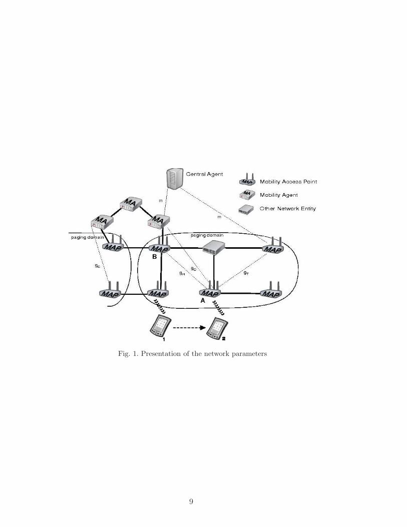
Fig. 1. Presentation of the network parameters

9

It is an NP full problem to calculate the optimal cell structure, but there arealgorithms approaching it very good in some sense. For example [16] solvesthis problem under additional constraints and limits the maximal paging cost.In our numerical simulation we have run the algorithms developed and pub-lished in [14] and obtained gC with them. However, concerning the NP fullnesstwo important notes have to be mentioned. When talking about an existingnetwork, these parameters can be calculated easily. If we work with small net-work patterns, the optimal cell structure can be selected from the not toomany options.

3.3 Modelling the Mobile Node

As we have seen, matrix BQ describes the movement behavior of the MN,handover-wise. If one sums up the ith row in this matrix it gets a rate howfrequent the MN moves from the ith MA (MAP) with a Poisson-process. Letλ denote the average parameter of the Poisson-process (at each MAP) and sodenote the rate of handovers for a general MN anywhere in the network.

The other parameter that can be introduced in a similar manner is the rateof receiving a call: µ. This parameter can also be time- or location-dependent.We take its average value as we did in the case of λ and we assume it isconstant in the examined very small time interval just like we did in the caseof matrix BQ and through the whole modelling.

Using the achievements in [8], let us introduce ρ as the ”mobility ratio” mean-ing the probability that the MN changes its FA before a call arrives. The goodthing in our notation is that various movement modelling can be embeddedinto it with varying BQ.

3.4 Loop Removal Effect and Moving Within a Subset of MAPs

We include the movement directions of the mobile node because many proto-cols try to exploit the advantage of returning to the a previous point of attach-ment or staying within a range of nodes. The first gives significant advantage oftracking protocols while the second has the effect on the performance on everyprotocol especially on the cellular approaches except the centralized-like ones.The loop removal is discussed within the optimization of the Tracking-likeand Cellular-like protocols. We use the achievement presented in our previouswork on LTRACK mobility management [8]. Returning to a subset of node isstill open for investigations but party incorporated to the problem of PagingArea decisions where we used one of our colleagues‘ method [14].

10

3.5 Definitions of Cost Constants

The three main classes of cost types and the corresponding cost constantsthat can describe the technology level will be introduced here. Why do weneed distinguished cost types?

The main reason is that the same kind of protocol can be implemented onvarious network layers that influences its signalling and processing needs ofeach protocol message. Another reason to introduce such network topology andmobility strategy independent cost constants is that the underlying networkingequipments might have very different characteristics so it might be importantto test the behavior of the Mobility Management System on different servingnetworks to find the most suitable one. For these reasons, one will always haveto tune these parameters according to the very implementation used. For ournumerical example values see Section 5 where we also show that modifyingthe ratio of some (or some set of) parameters (for example the registrationand packet forwarding cost) strongly affect the performance of a mobilitymanagement system.

3.5.1 Link Related Constants

First class of the cost constants are the “link related constants” (see. Table 1).They are introduced since one of the most important properties of a network isthe bottleneck of uplink and downlink bandwidth especially when the servicehas to satisfy Quality of Service (QoS) requirements as well.

As it was described, our network model does not necessarily show the realnetwork topology. Each edge in the graph denotes the link from one MA toanother. There might be several routers and subnetworks among the path. Theparameters introduced here gives one unit signalling cost in each direction.

3.5.2 Node Related Constants

The “node related constants” model the cost of resources in the MA nodes(the vertices of our graph). For example the cost of creating a packet mightbe different for different protocols (number of headers, if there is tunnelling,etc.) so these constants should be adopted to the examined protocol but alsomight be different using equipments of different vendors too.

11

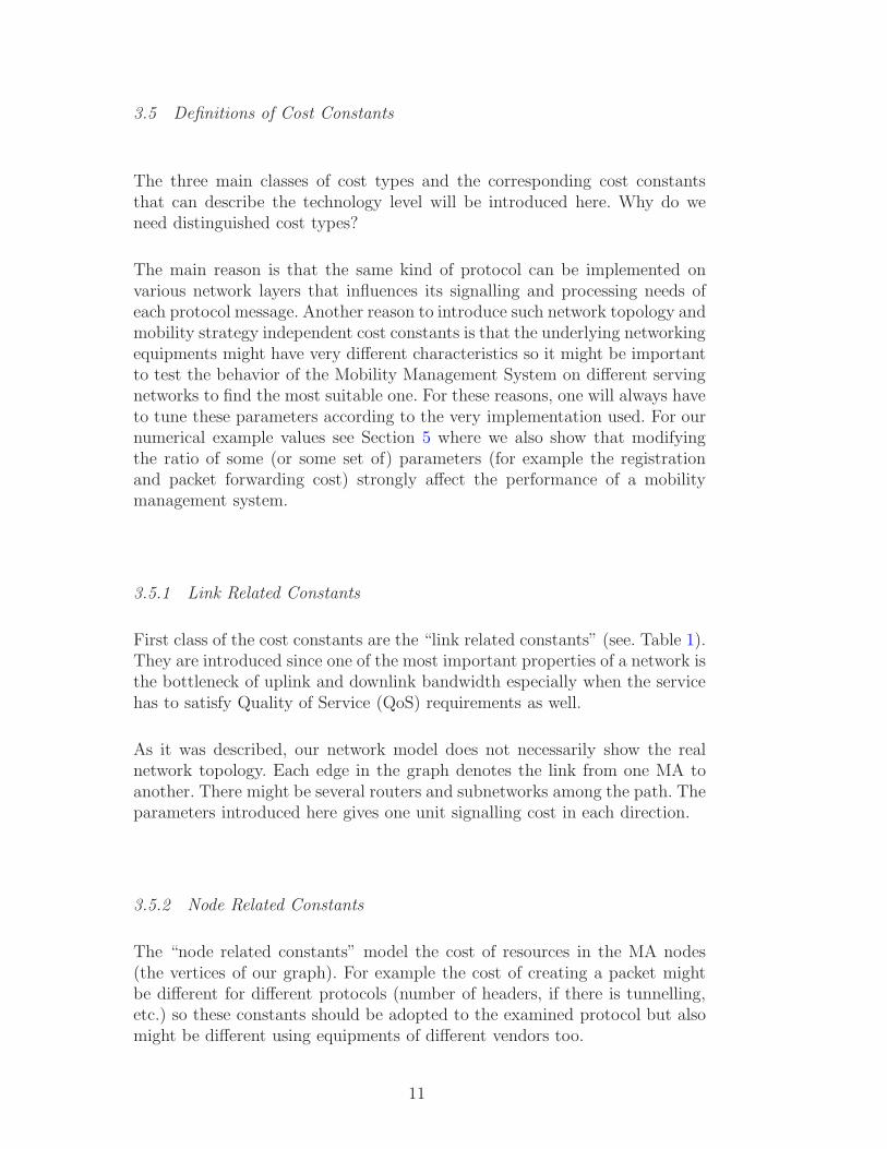
Table 1The cost contants

Signalling cu The unit cost of one update on a link.

constants cd The unit cost of one delivery on a link.

Processing cr Registration cost, the cost of the process in the MAP

constants when a MN node wants to attach.

cf Forwarding cost at a MA.

cm This is the constant cost of modifying some node

related records in a MA.

cec The cost of building up a message.

crc The cost of recapsulating or rebuliding a message.

cdc The cost of decapsulate or open the message at an endpoint.

In many cases crc = cdc + cec.

Air if. cau The cost of uplink message between the MN and the MAP.

constants cad The cost of downlink messaging between the MN

and the MAP.

3.5.3 Mobile Equipment Connection Related Constants

The “access interface and connection related constants” will denote of theunit cost of using the “access interface”. This access interface can denoteradio access or the cost when one connects his laptop to an ethernet cable andthere is load on the network from the laptop (MN) to the MAP (server of thenetwork). We will collect the costs of this group of tasks in two parameters:upload and download.

It is easy to see that the cost might be different for upload, download especiallyif download is a simple broadcasted paging (mainly MAP resources needed)while upload is a registration message that needs more resource (battery)at the MN side. As we mentioned in Section 3.1 the layer 2 handoff costs,for example the movement detection, Access Point (AP) searching, and APreassociation can be taken into account here.

3.5.4 Example for cost diversification

Here we try to underpin the above classification theoretically. We want togive an example but of course many kinds of setups are possible. When aMN moves (leaves its old MAP and connects to a new one) different eventshappens in layer 2 and layer 3. The costs of these events, the layer 2 handoff,the agent discovery and the actual registration are incorporated to interfaceand air interface cost in our paper. The first one depends on the access tech-nology and can be accomplished in different ways. For example in the case ofIEEE 802.11b WLAN it means the AP changes, and can be split into threeparts: movement detection, AP searching, and AP reassociation. In order tohandle this difference of layer 2 handoff of access technology we can take

12

into account this cost using an average layer 2 handoff cost. Agent discoveryis another process in layer 3, during this phase, the Mobility Access Pointadvertises their services on the network by using a Discovery Protocol forexample ICMP Router Discovery Protocol (IRDP) in Mobil IP. The MobileNode listens to these advertisements to determine where it is connected to, orif it is connected to its home network or foreign network. The Discovery Pro-tocol advertisements can carry the types of services MAP will provide such asreverse tunneling and Generic Routing Encapsulation (GRE) and the allowedregistration lifetime or roaming period for visiting Mobile Nodes. Rather thanwaiting for agent advertisements, a Mobile Node can send out an agent solic-itation. This solicitation forces any agents on the link to immediately send anagent advertisement. When the Mobile Node hears an Agent advertisementand detects that it has moved outside of its last network then registers itscurrent location during registration process.

4 Modelling the Existing Approaches

In this Section, the five main classes of mobility management protocols intro-duced in Section 2 are shortly described and modelled with their signalling-,processing-, and air interface cost functions.

The cost function as the model for the mobility approach can be any kindof utility function depending on the purpose of use. It is constructed as acalculation of expected utility as a function of network topology descriptorsand cost constants with respect to mobility i.e. the conditioned probability ofchanging the attachment point with λ(MAPij , t) intensity on not being pagedwith µ(t) intensity generally:

C =E[

∞∫

−∞

fh(n, c)dP (λ(MAPij, t)) (4)

+

∞∫

−∞

fp(n, c)dP (µ(t))],

where λ, µ are the intensities of a Poisson process and n ∈ {“network parameters”}, c ∈{“technology constants”}. Functions fh, fp are unique for each mobility man-agement strategy and mostly are a linear function of the network parametersand the technology constants. They tell us the cost of one handover or onepaging for each protocol respectively. Since the integral is taken with respectto a Poisson process it will be a simple sum and with introducing the handover

13

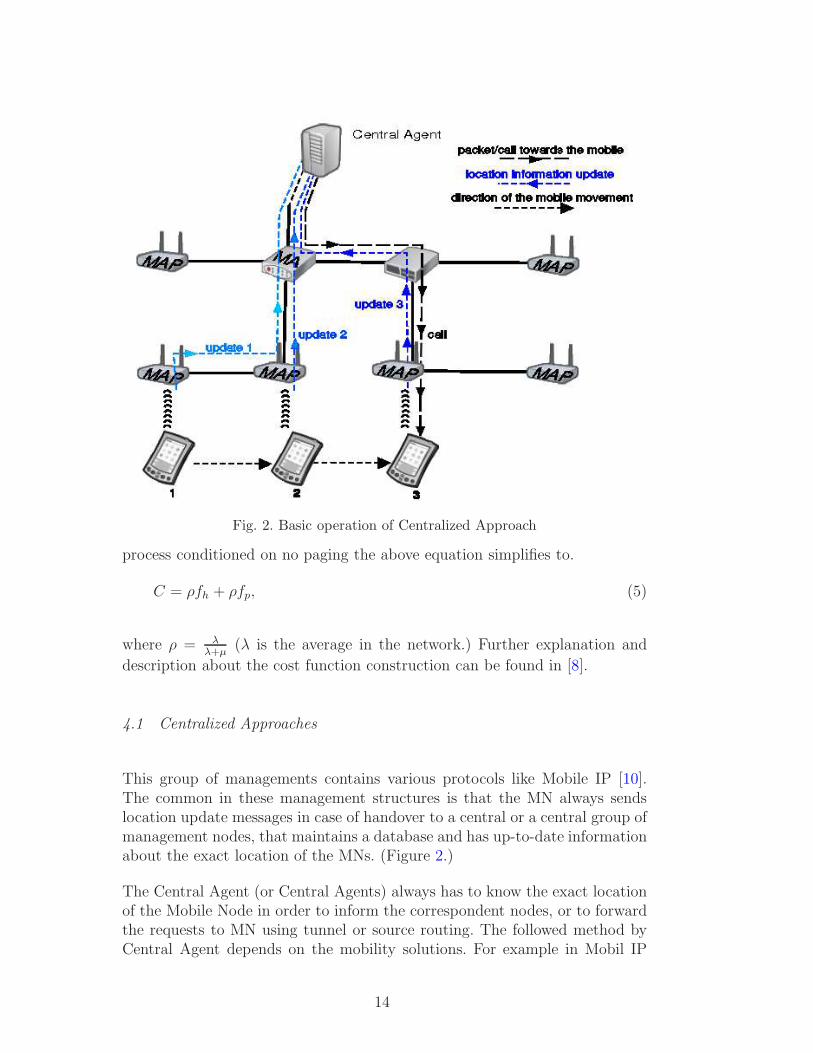
Fig. 2. Basic operation of Centralized Approach

process conditioned on no paging the above equation simplifies to.

C = ρfh + ρfp, (5)

where ρ = λλ+µ

(λ is the average in the network.) Further explanation and

description about the cost function construction can be found in [8].

4.1 Centralized Approaches

This group of managements contains various protocols like Mobile IP [10].The common in these management structures is that the MN always sendslocation update messages in case of handover to a central or a central group ofmanagement nodes, that maintains a database and has up-to-date informationabout the exact location of the MNs. (Figure 2.)

The Central Agent (or Central Agents) always has to know the exact locationof the Mobile Node in order to inform the correspondent nodes, or to forwardthe requests to MN using tunnel or source routing. The followed method byCentral Agent depends on the mobility solutions. For example in Mobil IP

14

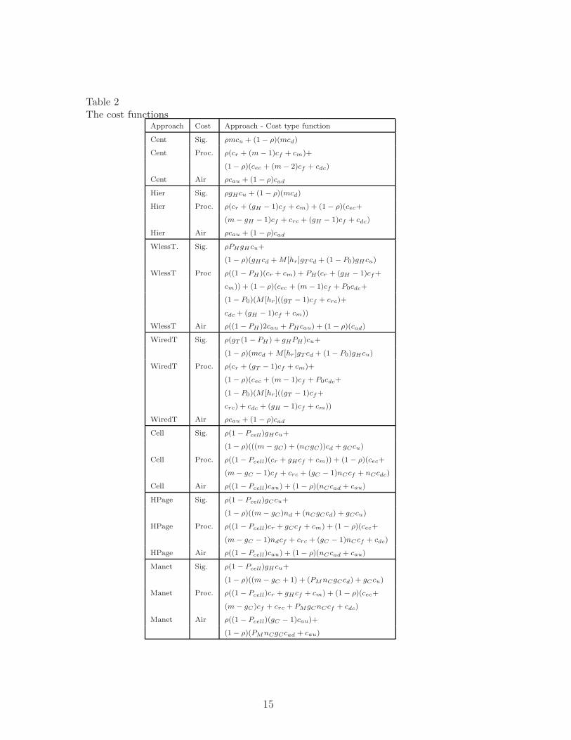
Table 2The cost functions

Approach Cost Approach - Cost type function

Cent Sig. ρmcu + (1− ρ)(mcd)

Cent Proc. ρ(cr + (m− 1)cf + cm)+

(1− ρ)(cec + (m− 2)cf + cdc)

Cent Air ρcau + (1 − ρ)cad

Hier Sig. ρgHcu + (1− ρ)(mcd)

Hier Proc. ρ(cr + (gH − 1)cf + cm) + (1− ρ)(cec+

(m− gH − 1)cf + crc + (gH − 1)cf + cdc)

Hier Air ρcau + (1 − ρ)cad

WlessT. Sig. ρPHgHcu+

(1− ρ)(gHcd +M [hr]gT cd + (1 − P0)gHcu)

WlessT Proc ρ((1 − PH )(cr + cm) + PH(cr + (gH − 1)cf+

cm)) + (1− ρ)(cec + (m − 1)cf + P0cdc+

(1− P0)(M [hr ]((gT − 1)cf + crc)+

cdc + (gH − 1)cf + cm))

WlessT Air ρ((1 − PH )2cau + PHcau) + (1− ρ)(cad)

WiredT Sig. ρ(gT (1 − PH ) + gHPH)cu+

(1− ρ)(mcd +M [hr]gT cd + (1− P0)gHcu)

WiredT Proc. ρ(cr + (gT − 1)cf + cm)+

(1− ρ)(cec + (m− 1)cf + P0cdc+

(1− P0)(M [hr ]((gT − 1)cf+

crc) + cdc + (gH − 1)cf + cm))

WiredT Air ρcau + (1 − ρ)cad

Cell Sig. ρ(1− Pcell)gHcu+

(1− ρ)(((m − gC) + (nCgC))cd + gCcu)

Cell Proc. ρ((1 − Pcell)(cr + gHcf + cm)) + (1− ρ)(cec+

(m− gC − 1)cf + crc + (gC − 1)nCcf + nCcdc)

Cell Air ρ((1 − Pcell)cau) + (1− ρ)(nCcad + cau)

HPage Sig. ρ(1− Pcell)gCcu+

(1− ρ)((m − gC)nd + (nCgCcd) + gCcu)

HPage Proc. ρ((1 − Pcell)cr + gCcf + cm) + (1− ρ)(cec+

(m− gC − 1)ndcf + crc + (gC − 1)nCcf + cdc)

HPage Air ρ((1 − Pcell)cau) + (1− ρ)(nCcad + cau)

Manet Sig. ρ(1− Pcell)gHcu+

(1− ρ)((m − gC + 1) + (PMnCgCcd) + gCcu)

Manet Proc. ρ((1 − Pcell)cr + gHcf + cm) + (1− ρ)(cec+

(m− gC)cf + crc + PMgCnCcf + cdc)

Manet Air ρ((1 − Pcell)(gC − 1)cau)+

(1− ρ)(PMnCgCcad + cau)

15

protocol the Home Agent as a Central Agent, forwards the packets usingtunnel, but in SIP based mobility the Registrar server answers the IP addressof MN to the SIP Proxy, which controls the communication.

As we have just seen on Table 2 the cost functions are obvious and simple. Inthe processing function there is only one encapsulation, one decapsulation andm − 2 forwarding cost, which do not need a big computative capacity. Theapplication of such a protocol has a second main advantage along with itssimplicity, namely these approaches can be built by installing a Central Agentin the network and by running an IP-level software module on the MN. Thereis no need to change any other entity in the network, therefore it is cheap andeasily installable. But we have to take a relevant disadvantage into account,centralized mobility puts extraordinary high overload on the bearer networkand uses non optimal routing, which are unacceptable. However, this solutionis far from the optimal, still the most of the mobility implementations use thesame kind of this centralized approach. Transport layer mobility, for examplemSCTP (multi-homing Stream Control Transmission Protocol), HIP and Ap-plication layer mobility for example SIP, as it was mentioned above, belongto this centralized approach. (The mSCTP allows an association between twoend points to span multiple IP addresses or network interface cards. It sup-ports to keep alive the TCP sessions during IP address change. HIP separatethe node identification and location information in the network layer. Thissolution affords the applications a permanent network layer. SIP provide thepossibility of many Voice over IP services.)

Despite these advantages all of these protocols need a centralized managementto accomplish the mobility, which is far from the efficiency it could have.

4.2 Hierarchical Solutions

Instead of the global management node regional management system can beused to reduce the signalling traffic by maintaining the location informationlocally. For this reason we can use the MAPs and MAs as local agents, thathave database to store the actual IP addresses of MN. So we can considerthis hierarchical network structure as a tree of MAP, MA and other networknode with Central Agent in the root of the tree. The main idea is that theupdate information is sent only to the nearest MA on the network, if the MNmoves within the subnetwork managed by this entity. Parameter gH denotesthis distance as it is explained in Section 3.2.5.

Let us now take a look at the network tree of the hierarchical mobility. Onepath from the HA leads to the old MA of the MN and another one leads tothe new one. It is enough to send the location update message to the nearest

16

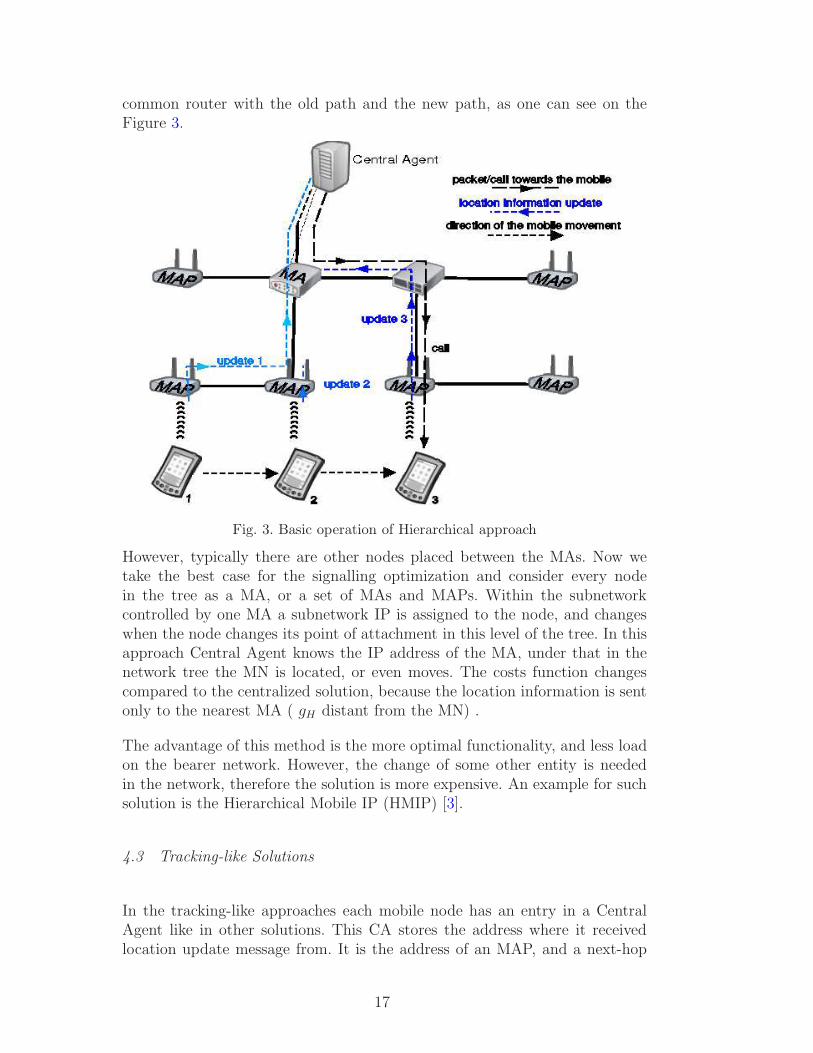
common router with the old path and the new path, as one can see on theFigure 3.

Fig. 3. Basic operation of Hierarchical approach

However, typically there are other nodes placed between the MAs. Now wetake the best case for the signalling optimization and consider every nodein the tree as a MA, or a set of MAs and MAPs. Within the subnetworkcontrolled by one MA a subnetwork IP is assigned to the node, and changeswhen the node changes its point of attachment in this level of the tree. In thisapproach Central Agent knows the IP address of the MA, under that in thenetwork tree the MN is located, or even moves. The costs function changescompared to the centralized solution, because the location information is sentonly to the nearest MA ( gH distant from the MN) .

The advantage of this method is the more optimal functionality, and less loadon the bearer network. However, the change of some other entity is neededin the network, therefore the solution is more expensive. An example for suchsolution is the Hierarchical Mobile IP (HMIP) [3].

4.3 Tracking-like Solutions

In the tracking-like approaches each mobile node has an entry in a CentralAgent like in other solutions. This CA stores the address where it receivedlocation update message from. It is the address of an MAP, and a next-hop

17

towards the mobile node. The mobile node is either still connected to thatMAP, or that MAP knows another next-hop MAP towards the mobile. Finallythe mobile node can be found at the end of a chain of MAPs.

As it was introduced the main idea behind the tracking-like algorithm is thatif the MN changes its point of attachment then it could be a good solution tosend an update to the old MAP. The MAP that the mobile node moves awayis called old MAP, the one it moves to is called new MAP. After this handover,called tracking handover the old MAP is able to forward the request towardsthe MN via the new MAP.

There is another kind of handover in tracking-like solutions, the normal han-dover. Normal handover occurs when mobile equipment updated its entry inthe Central Agent by sending the address of the new MAP node to it.

The normal handover is similar to centralized solutions; it generates a lot ofsignalling traffic, but a tracking handover puts less, or no signaling to thenetwork (see Section 4.3.2 and 4.3.1). But if an incoming packet arrives tothe mobile node, we have to find it in a hop-by-hop manner, and send alocation update message to the Central Agent, which are expensive. In trackingscheme a normal handover can be followed by some tracking handovers beforeanother normal handover takes place. If the mobile node does not receive apacket between two normal handovers then less signalling is used, if a packetis received after some tracking handovers, more signalling is used comparedto a centralized mobility scheme.

Thus the most important decision of tracking-like mobility is when to makea normal handover, and when to make a tracking handover. In the tracking-like approaches each mobile node has an entry in a Central Agent like inother solutions. This CA stores the address where it received location updatemessage from. It is the address of an MAP, and is a next-hop towards themobile node. The mobile node is either still connected to that MAP, or thatMAP knows another next-hop MAP towards the mobile. Finally the mobilenode can be found at the end of a chain of MAPs. One can read more aboutthese protocols in works: [1], [12], [8].

We distinguish between two different tracking-like solutions based on the kindof tracking handover: wireless tracking and wired tracking. In case of track-ing handover of wireless tracking the mobile sends the address of the newMAP node to the old MAP node over the air interface (for reference seeLTRACK [8]) while in case of the wired tracing the information is sent overthe wired network [12].

The optimal number of tracking handovers between two normal handovers hasto be calculated in both cases. We use the achievements in [8] to determinethese parameters and define the optimal cost function. The model and the

18

effect of loop-removal is imported to our work as well.

4.3.1 Wireless Tracking

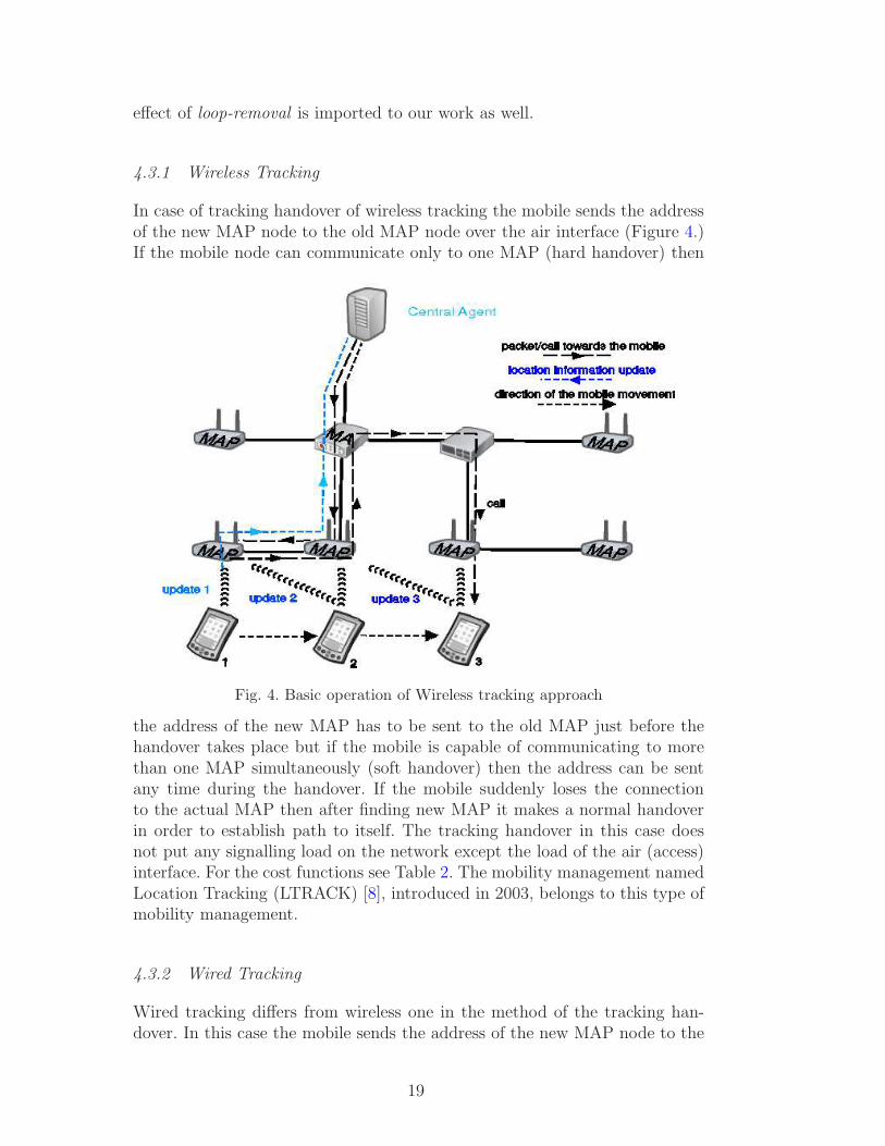
In case of tracking handover of wireless tracking the mobile sends the addressof the new MAP node to the old MAP node over the air interface (Figure 4.)If the mobile node can communicate only to one MAP (hard handover) then

Fig. 4. Basic operation of Wireless tracking approach

the address of the new MAP has to be sent to the old MAP just before thehandover takes place but if the mobile is capable of communicating to morethan one MAP simultaneously (soft handover) then the address can be sentany time during the handover. If the mobile suddenly loses the connectionto the actual MAP then after finding new MAP it makes a normal handoverin order to establish path to itself. The tracking handover in this case doesnot put any signalling load on the network except the load of the air (access)interface. For the cost functions see Table 2. The mobility management namedLocation Tracking (LTRACK) [8], introduced in 2003, belongs to this type ofmobility management.

4.3.2 Wired Tracking

Wired tracking differs from wireless one in the method of the tracking han-dover. In this case the mobile sends the address of the new MAP node to the

19

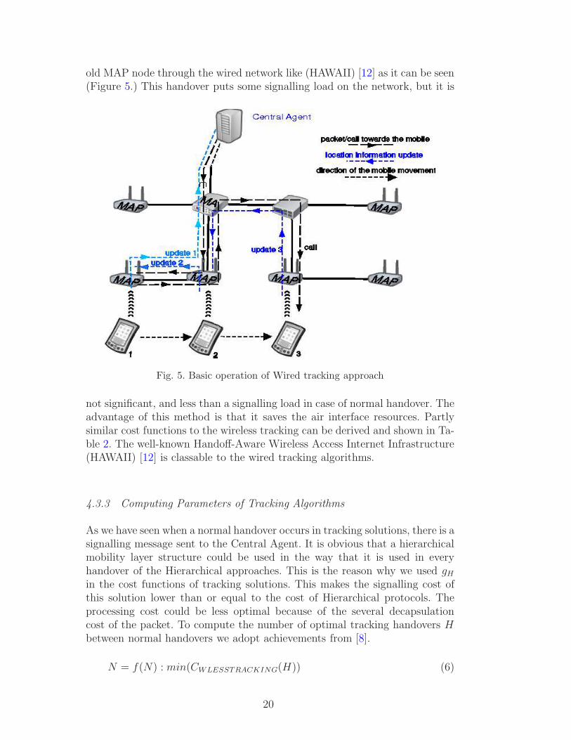
old MAP node through the wired network like (HAWAII) [12] as it can be seen(Figure 5.) This handover puts some signalling load on the network, but it is

Fig. 5. Basic operation of Wired tracking approach

not significant, and less than a signalling load in case of normal handover. Theadvantage of this method is that it saves the air interface resources. Partlysimilar cost functions to the wireless tracking can be derived and shown in Ta-ble 2. The well-known Handoff-Aware Wireless Access Internet Infrastructure(HAWAII) [12] is classable to the wired tracking algorithms.

4.3.3 Computing Parameters of Tracking Algorithms

As we have seen when a normal handover occurs in tracking solutions, there is asignalling message sent to the Central Agent. It is obvious that a hierarchicalmobility layer structure could be used in the way that it is used in everyhandover of the Hierarchical approaches. This is the reason why we used gHin the cost functions of tracking solutions. This makes the signalling cost ofthis solution lower than or equal to the cost of Hierarchical protocols. Theprocessing cost could be less optimal because of the several decapsulationcost of the packet. To compute the number of optimal tracking handovers Hbetween normal handovers we adopt achievements from [8].

N = f(N) : min(CWLESSTRACKING(H)) (6)

20

For the basic model the cost functions of wireless tracking can be treated asa continuous one and can be derived. This provides a fast and easy solutionfor computing the optimal value of H with taking looping into account aswell. If we extend our model with the effect of loop removal, it is clear thatthe cost function for tracking approaches remains the same, but values of thestate probabilities (PH , P0), and the expected point of return (M [hr]) will bedifferent.

4.4 Cellular-like Solutions

To mobility problem there are cellular-like solutions as well. One well-knownexample is Cellular IP (CIP) [2]. The idea behind this kind of approach comesfrom the GSM protocol. Basically this kind of protocols can be used in lowerlevel of the hierarchical network.

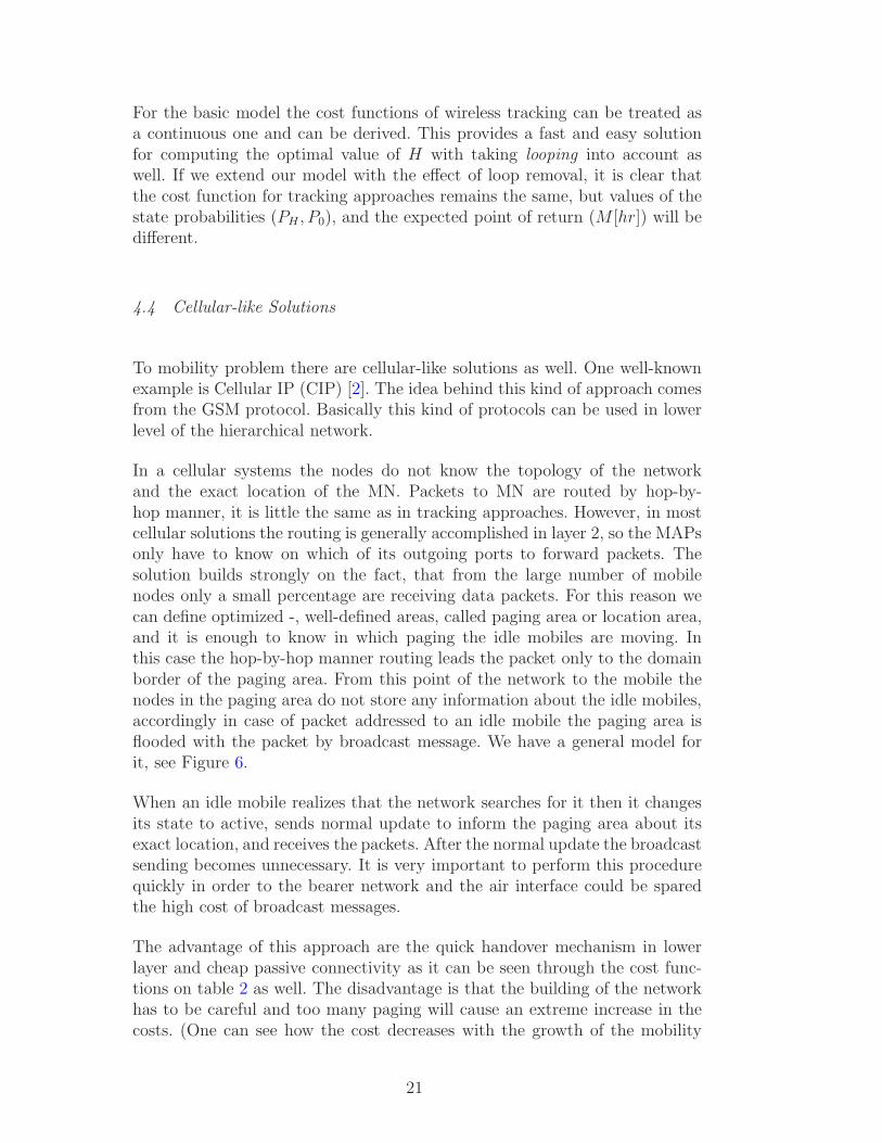
In a cellular systems the nodes do not know the topology of the networkand the exact location of the MN. Packets to MN are routed by hop-by-hop manner, it is little the same as in tracking approaches. However, in mostcellular solutions the routing is generally accomplished in layer 2, so the MAPsonly have to know on which of its outgoing ports to forward packets. Thesolution builds strongly on the fact, that from the large number of mobilenodes only a small percentage are receiving data packets. For this reason wecan define optimized -, well-defined areas, called paging area or location area,and it is enough to know in which paging the idle mobiles are moving. Inthis case the hop-by-hop manner routing leads the packet only to the domainborder of the paging area. From this point of the network to the mobile thenodes in the paging area do not store any information about the idle mobiles,accordingly in case of packet addressed to an idle mobile the paging area isflooded with the packet by broadcast message. We have a general model forit, see Figure 6.

When an idle mobile realizes that the network searches for it then it changesits state to active, sends normal update to inform the paging area about itsexact location, and receives the packets. After the normal update the broadcastsending becomes unnecessary. It is very important to perform this procedurequickly in order to the bearer network and the air interface could be sparedthe high cost of broadcast messages.

The advantage of this approach are the quick handover mechanism in lowerlayer and cheap passive connectivity as it can be seen through the cost func-tions on table 2 as well. The disadvantage is that the building of the networkhas to be careful and too many paging will cause an extreme increase in thecosts. (One can see how the cost decreases with the growth of the mobility

21

Fig. 6. Basic operation of Cellular approach

ratio ρ in Section 5.)

4.4.1 Cellular-like Systems

The Cellular IP (CIP) is not the only one that uses the GSM like solutionfor mobility management. We will present another micro-mobility protocolbased on the MANET [6] that uses the technique of wireless ad-hoc networks.However, the algorithm can be extended to macro-mobility level too and thusHierarchical Paging [7] is introduced as an alternative Mobility Managementsolution.

The ”MANET [6] in the paging areas” solutions introduced by us could be thebest solution when we would like to save the infrastructure cost and the airinterface using is cheaper. In this management system it is assumed that allMN could be reached via other MNs. Paging areas are defined like in other cell-like solutions, but only one MAP exists in one page, through this the packetsare routed using an optimal MANET algorithm. Advantage of this solutionalso is that signaling cost can be saved with correct MANET protocol in apage. However, in the suboptimal case some mobiles could not be reached,and aggregate air interface cost can be high.

The main idea behind the Hierarchical Paging [7] is that not only the lowerlayer network is flooded with the packet but broadcast message is used to find

22

0.2 0.4 0.6 0.8 1Ρ

7.5

10

12.5

15

17.5

20

22.5

COST

0.2 0.4 0.6 0.8 1Ρ

7.5

10

12.5

15

17.5

20

22.5

COST

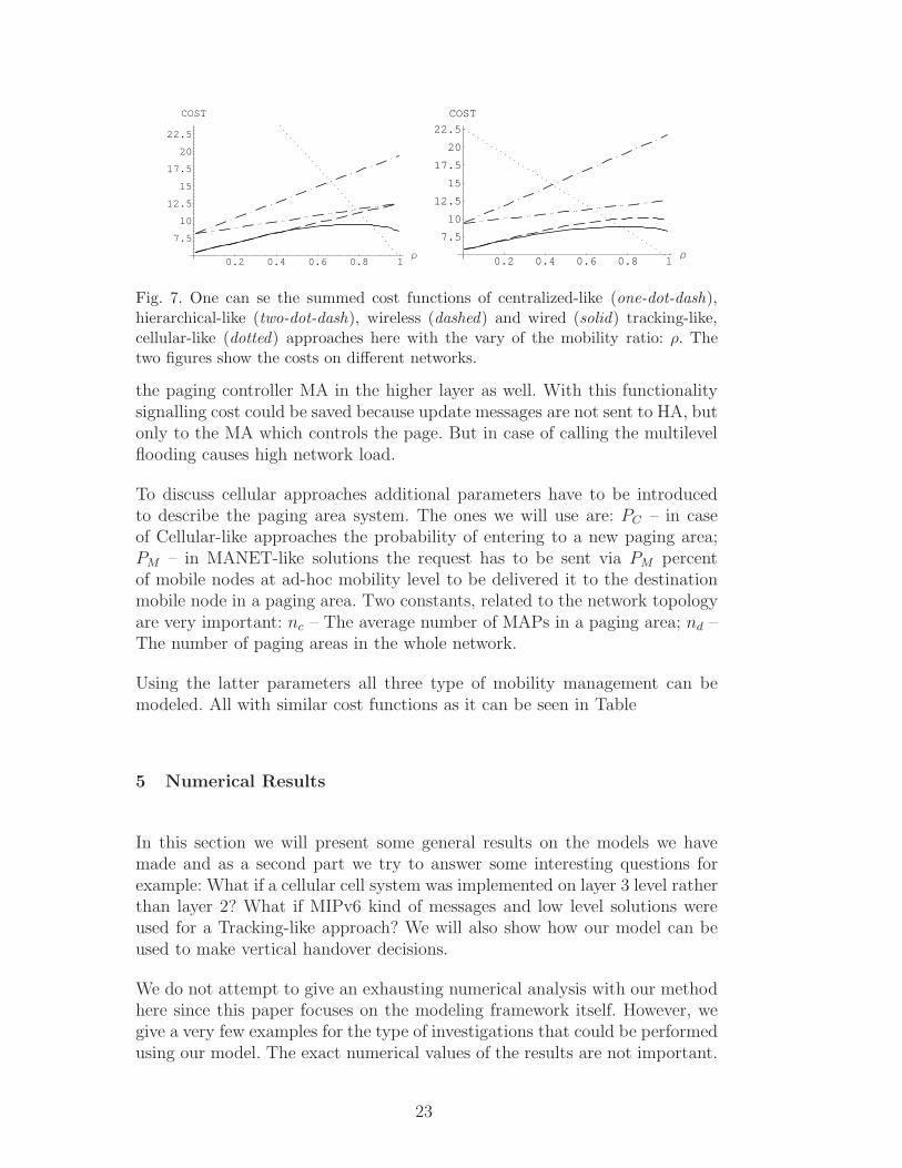
Fig. 7. One can se the summed cost functions of centralized-like (one-dot-dash),hierarchical-like (two-dot-dash), wireless (dashed) and wired (solid) tracking-like,cellular-like (dotted) approaches here with the vary of the mobility ratio: ρ. Thetwo figures show the costs on different networks.

the paging controller MA in the higher layer as well. With this functionalitysignalling cost could be saved because update messages are not sent to HA, butonly to the MA which controls the page. But in case of calling the multilevelflooding causes high network load.

To discuss cellular approaches additional parameters have to be introducedto describe the paging area system. The ones we will use are: PC – in caseof Cellular-like approaches the probability of entering to a new paging area;PM – in MANET-like solutions the request has to be sent via PM percentof mobile nodes at ad-hoc mobility level to be delivered it to the destinationmobile node in a paging area. Two constants, related to the network topologyare very important: nc – The average number of MAPs in a paging area; nd –The number of paging areas in the whole network.

Using the latter parameters all three type of mobility management can bemodeled. All with similar cost functions as it can be seen in Table

5 Numerical Results

In this section we will present some general results on the models we havemade and as a second part we try to answer some interesting questions forexample: What if a cellular cell system was implemented on layer 3 level ratherthan layer 2? What if MIPv6 kind of messages and low level solutions wereused for a Tracking-like approach? We will also show how our model can beused to make vertical handover decisions.

We do not attempt to give an exhausting numerical analysis with our methodhere since this paper focuses on the modeling framework itself. However, wegive a very few examples for the type of investigations that could be performedusing our model. The exact numerical values of the results are not important.

23

-2 -1 1 22fel7.5

10

12.5

15

17.5

20

22.5

COST

-2 -1 1 22fel

10

12

14

16

18

20

COST

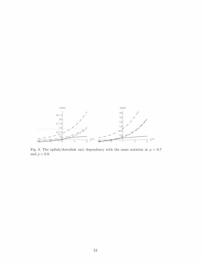
Fig. 8. The uplink/downlink vary dependency with the same notation at ρ = 0.7and ρ = 0.9.

24

We focus on the behavior of mobility with the change of the parameters.

5.1 General Differences Between Management Approaches

On Fig. 7 one can see the difference between the approaches considering allthe cost types (signalling, processing, air). It is clear that with the bigger fre-quency of handovers (ρ) the cost is bigger for the centralized-like, hierarchical-like and wired tracking-like approaches since each handover gives more sig-nalling on the network. In the wireless tracking-like case if the number ofhandovers rise between the incoming calls it starts to save the costs of thererouting of the packets. In the centralized-like ones, it is clear that the rarerthere is an incoming call the less load the network has. The cost is obviouslyhigh in these case. The same case is printed on both figures, but the valuesof gT , gC network parameters are significantly less than gH (more meshed net-work). One can see that the wired tracking-like solution is getting cheaper aswell and begins to behave as its tracking-like pair.

On Fig. 8 the mobility ratio is fixed to (ρ = 0.7, ρ = 0.9) respectively. Onthe other hand the cost of a single upload (cu) to a single download (cd) isexponentially changing from the half to the twice on the horizontal axis. Mostof the solutions are more expensive if the upload is higher but it can be seenthat the wireless tracking cuts this cost as expected.

5.2 Technology Tendency via Cost Constants and Simulation

To answer questions like ”What if a strategy like a cellular approach was imple-mented on a different technology level, we should give clear values of the costconstants. To do this we build up a simulation environment. OMNet++ [18]was used, which is a public-source, component-based, simulation environmentwith strong GUI support and an embeddable kernel. We have realized four IPlayer mobility management, Mobile IPv4, Mobile IPv6 and our previous pro-posal, LTRACK on IPv4 and IPv6. We expect different technology constantsfor the two types of Internet Protocol however it is also unavoidable that twodifferent kind of realized protocols differ in the constant values. During thesimulation develop we followed strictly the protocols description and the resultis presented in Table 3.

Shortly discussing the results we would like to point out an example. Taking alook at Table 3 it can be seen that in the case of MIPv6 the encapsulation cost(cec) is lower because there is no “triangle communication” instead it uses themechanism of constantly updated “binding caches” while the registration cost(cd) is higher because the IPv6 protocol overhead itself is higher. These facts

25

Table 3The cost constants of different technology levels from the simulation.

Cost type MIPv4 MIPv6 LTRACKv4 LTRACKv6

cu 499 777 481 695

cd 1825 1821 1814 1843

cr 187 1068 711 821

cf 652 685 636 690

cm 543 1239 538 541

cec 240 234 237 239

crc 0 0 235 238

cdc 240 234 240 240

cau 136 181 138 165

cad 390 396 368 397

2 4 6 8 10p�s

10000

20000

30000

40000

COST

2 4 6 8 10a�s

4000

6000

8000

COST

Fig. 9. The left Figure represents the cost of protocols in the ratio of “processing”and “signalling” costs while the right does the same in the ratio of “accessing” and“signalling” again.

intuitively verify our simulations. To prove the applicability of the simulationto our model framework we ran it on different network topologies and mo-bile movement setups and derived the expected value of each. With long runsimulations the distribution concentrated near to the mean with low variationwhat proves the fact that these technology related constants are network andalgorithm independent. (The network dependent cost constants for examplethe bandwidth measures are given in the weighted adjacency matrix A.)

In addition to the table above one is supposed to weight each type (“process-ing”, “signalling”, “accessing”) of cost with different values since the cost ofbandwidth is not in the same measure as the cost of processor load for ex-ample. On Figure 9 it can be followed for each how the cost of the mobilitychanges with the ratio of “processing” and “signalling” then the ratio of “ac-cessing” and “signalling” cost respectively. If we know that in the future themobile equipments and accessing technologies will become relatively cheap tothe signaling resources then Figure 9 tells us that the ... protocol saves rela-tively the most with this tendency (of course on the given network and withthe given implementation with the given mobility parameters, etc.).

26

5.3 How to Use the Model for Vertical Handover Decisions

We will present how to use our mobility management framework to make ver-tical handover decisions. Consider a vertical handover system of two protocolson the same region. The weights on network edges will denote the relative costof using the given protocol divided by the QoS it provides. As an example,let network “A” be a locally maintained university WLAN network that canbe used almost for free but provides bad QoS and network “B” be a GSMnetwork covering the same area which provides better QoS but expensive.The ratio of the relative cost in money and some QoS measure depends onthe user (or installed service). The network matrix than splits to two parts.One is for network “A” and the link weights (that basically shows relationsbetween all the links) are multiplied by the above ratio expressing the user(anti-)preference. If the value ratio value is higher then the user is less willingto use the network since it has the more basic cost.

To grab the meaning of the vertical handover decision we have to manipulatethe MN movement modeling part, the handover frequency matrix. If the net-work “A” is too expensive, then the total handovers from the network “B”are lower while backward handovers became higher expressing that the user ismore willing to stay at the preferred part. Of course topologically the mobilenodes have to move within a given network too if they are making handovers.

In Figure 10 we depict an example how the vertical handover decision can bemodeled within our framework. The two networks can be found on the top andthe bottom. The nodes can move within the access points (MAP) of a networkas a part of the normal operation. Note that the two Access network do notneed to cover the same geographical area instead where vertical handover ispossible we put a link into the Handover Frequency graph with ν and 1/ν foreach direction.

As one can realize we used a stochastic method to make vertical handoverdecisions. It is in the scope of our research to compare it to others but fornow we try to emphasize why a stochastic method should be applied throughan example. Suppose that the cost of a required QoS on the nodes are as it isdepicted on the graph on Figure 10. The total cost of QoS in access network“A” is higher than in “B”. On the other hand if the user mobility is higherthan while it receives less traffic it is much more worth to stay at network“A”. Since the mobility is a Poisson process, and the threshold depends on it(not just on its mean), it will vary according to a random variable too.

We used Mathematica for the implementation of the cost functions and themodeling and its capability for symbolic computations helps us to easily ma-nipulate those rows and columns in the handover frequency matrix which

27

Fig. 10. Vertical handover modelling example

28

1 2 3 4 5Η

18

20

22

24

26

1�Utility

0.2 0.4 0.6 0.8 1QoS�Cost

16

18

20

22

1�Utility

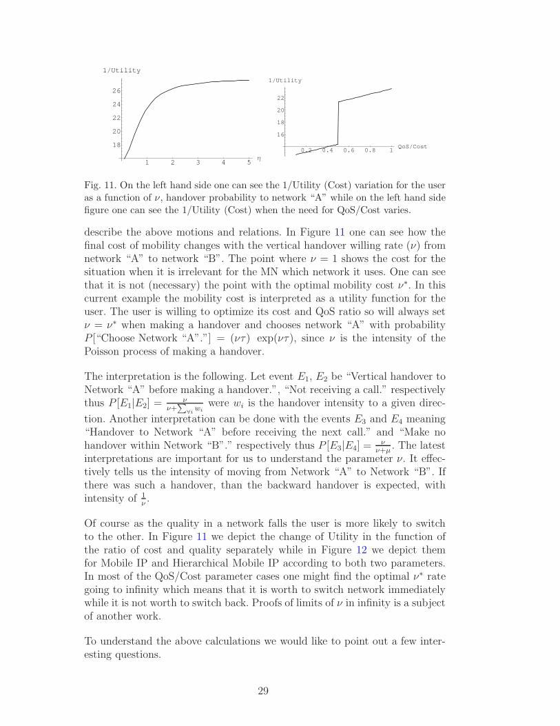
Fig. 11. On the left hand side one can see the 1/Utility (Cost) variation for the useras a function of ν, handover probability to network “A” while on the left hand sidefigure one can see the 1/Utility (Cost) when the need for QoS/Cost varies.

describe the above motions and relations. In Figure 11 one can see how thefinal cost of mobility changes with the vertical handover willing rate (ν) fromnetwork “A” to network “B”. The point where ν = 1 shows the cost for thesituation when it is irrelevant for the MN which network it uses. One can seethat it is not (necessary) the point with the optimal mobility cost ν∗. In thiscurrent example the mobility cost is interpreted as a utility function for theuser. The user is willing to optimize its cost and QoS ratio so will always setν = ν∗ when making a handover and chooses network “A” with probabilityP [“Choose Network “A”.”] = (ντ) exp(ντ), since ν is the intensity of thePoisson process of making a handover.

The interpretation is the following. Let event E1, E2 be “Vertical handover toNetwork “A” before making a handover.”, “Not receiving a call.” respectivelythus P [E1|E2] =

νν+

∑∀i

wiwere wi is the handover intensity to a given direc-

tion. Another interpretation can be done with the events E3 and E4 meaning“Handover to Network “A” before receiving the next call.” and “Make nohandover within Network “B”.” respectively thus P [E3|E4] =

νν+µ

. The latestinterpretations are important for us to understand the parameter ν. It effec-tively tells us the intensity of moving from Network “A” to Network “B”. Ifthere was such a handover, than the backward handover is expected, withintensity of 1

ν.

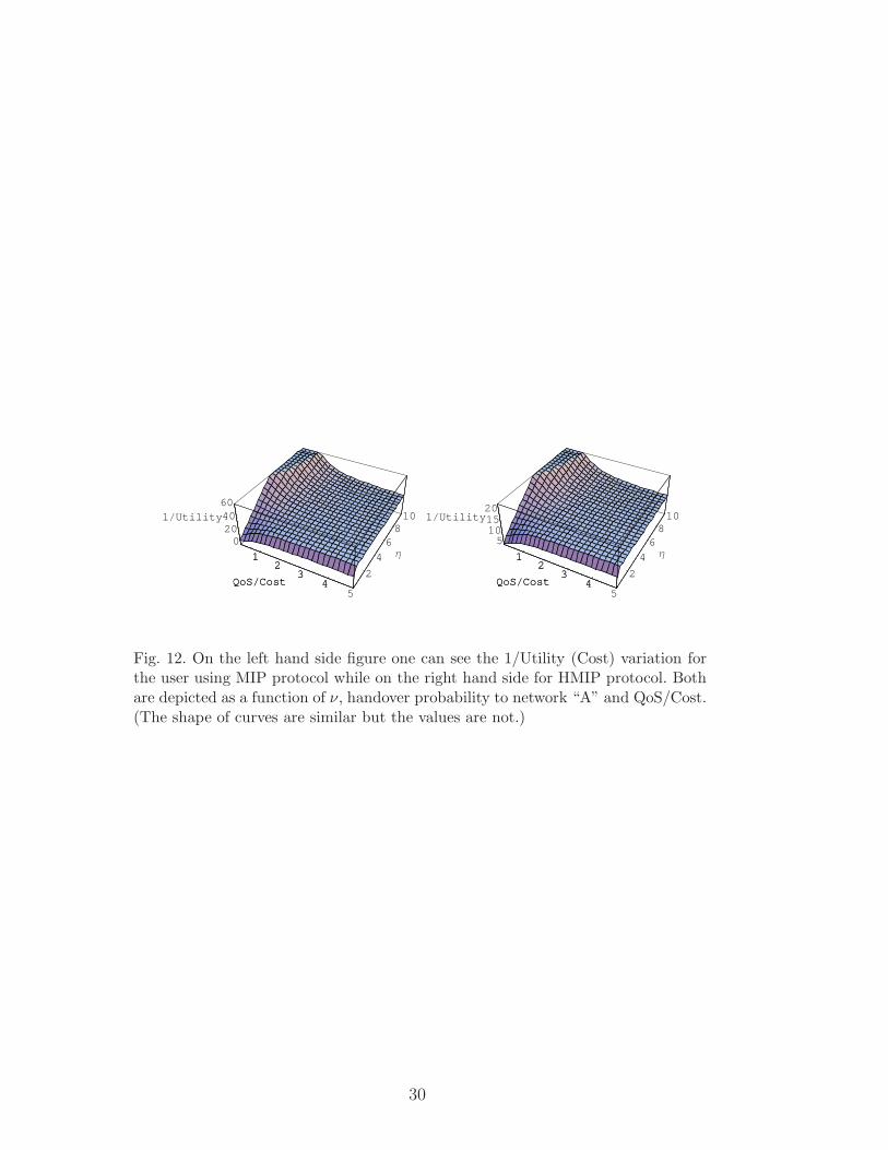
Of course as the quality in a network falls the user is more likely to switchto the other. In Figure 11 we depict the change of Utility in the function ofthe ratio of cost and quality separately while in Figure 12 we depict themfor Mobile IP and Hierarchical Mobile IP according to both two parameters.In most of the QoS/Cost parameter cases one might find the optimal ν∗ rategoing to infinity which means that it is worth to switch network immediatelywhile it is not worth to switch back. Proofs of limits of ν in infinity is a subjectof another work.

To understand the above calculations we would like to point out a few inter-esting questions.

29

12

34

5QoS�Cost

2

4

6810

Η

0204060

1�Utility

12

34

5QoS�Cost

12

34

5QoS�Cost

2

4

6810

Η

5101520

1�Utility

12

34

5QoS�Cost

Fig. 12. On the left hand side figure one can see the 1/Utility (Cost) variation forthe user using MIP protocol while on the right hand side for HMIP protocol. Bothare depicted as a function of ν, handover probability to network “A” and QoS/Cost.(The shape of curves are similar but the values are not.)

30

The first to answer is: ”How does the single network matrix and the derivedparameter m, gH , etc. differentiate between the two networks?” The answer isit does via the stationary distribution of the Mobile Nodes. If the ν is highthan handover rate from Network “A” to “B” is much higher than backwards.This means that the MNs spend more time at the Access Points of Network“B”. When we calculate m we multiply the shortest paths in the networkgraph with this probability distributions thus paths with higher Utility (thepaths of Network “B”) will have bigger weights that says we use them moreoften.

One might believe that the intensity of handovers to the network with thebigger Utility is higher than backwards but “Why do we have handovers tothe network with less Utility at all?”. The answer for this question is obvious:because we have used a Stochastic model. We have never stated that Network“A” is better than Network “B” in terms of QoS to Cost ratio, but we havestated that it is better with respect to the stochastic model we used (stochasticprocesses for both call arrival and handover rate). It is not a part of our currentwork to give analytical proof of the fact that our stochastic model is betterfor vertical handover decisions than existing deterministic ones.

6 Conclusions and Future Work

In this paper we grabbed numerous significant parameters of mobility andproposed a framework to model the mobile node behavior and the networkindependently of the very technology used. As an example we modeled somegeneral management strategies and obtained technology constants with simu-lations to give some analytical results. We showed how each modeled protocolresponds to tendencies in technology developments and trends and proposeda method to deal with vertical handover decisions using the framework. Withour work it could be shown which mobility management gives the best solu-tion in different given network scenarios and which aspect of resources couldbe a bottleneck in each case. This can help operators to tune the parame-ters of their systems, plan their networks and researchers to propose mobilitymanagement solutions of low cost.

Acknowledgements

Special thanks to the support from the High Speed Network Laboratory:http://www.tmit.bme.hu/labgroup/hsn!eng.

31

References

[1] Abondo, C., & Pierre, S., Dynamic Location And Forwarding Pointers ForMobility Management, 2005, Mobile Information Systems, IOS Press, 3-24.

[2] Campbell, A. T., Gomez, J., & Valko, A. G., An Overview of Cellural IP. 1999,IEEE., 29-34.

[3] Castelluccia, C., A Hierarchical Mobile IP Proposal, 1998, Inria TechnicalReport.

[4] Fang, Y., & Lin, Y., Portable Movement Modelling for PCS Networks, 2000,IEEE Transactions on Vehicular Technology, 1356-1362.

[5] Jokela, P., Nikander, P., Melen, J., Ylitalo, J., &Wall, J., Host Identity Protocol:Achieving IPv4 - IPv6 handovers without tunneling, 2003, Proceedings ofEvolute workshop, ”Beyond 3G Evolution of Systems and Services”, Universityof Surrey, Guildford, UK.

[6] Ashwini K. Pandey, Hiroshi Fujinoki, Study of MANET routing protocols byGloMoSim simulator International 2005, Journal of Network Management.

[7] Szalay, M., Imre, S., Hierarchical Paging - A novel location managementalgorithm, 2006, ICLAN’2006 International Conference on Late Advances inNetworks, Paris, France.

[8] Kovacs, B., Szalay, M., & Imre, S., Modelling and Quantitative Analysis ofLTRACK - A Novel Mobility Management Algorithm, 2006, Mobile InformationSystems, Issue: Volume 2, Number 1/2006, 21 - 50.

[9] Ma, W., & Fang, Y., Dynamic Hierarchical Mobility Management Strategy forMobile IP Networks, 2004, IEEE Journal of Selected Areas In Communications.

[10] Perkins, C. E., Mobile IP, 1997, IEEE Communications Magazine.

[11] Escalle, P. G., Giner, V. C., & Oltra, J. M., Reducing Location Updateand Paging Costs in a PCS Network, 2002, IEEE Transactions on WirelessCommunications, 200-209.

[12] Ramjee, R., La Porta, T., Thuel, S., Varadhan, K., & Salgarelli, L., AHierarchical Mobile IP Proposal, 1998, Inria Technical Report.

[13] S. Das, A., Misra, P. Agraval & S. K. Das, TeleMIP: Telecommunications-Enhanced Mobile IP Architecture for Fast Intradomain Mobility, 2000, IEEEPersonal Communications, 50-58.

[14] Vilmos Simon, Sndor Imre, Location Area Design Algorithms for MinimizingSignalling Costs in Mobile Networks, International Journal of Business Data,2007, Communications and Networking.

[15] Szalay, M., Imre, S., Hierarchical Paging- Efficient Location Management, 2007,Fourth European Conference on Universal Multiservice Networks (ECUMN’07),301-310.

32

[16] Vilmos Simon, Sndor Imre, A Paging Cost Constrained Location Area Planningin Next Generation Mobile Networks, 2006, The 4th International Conferenceon Advances in Mobile Multimedia- MoMM 2006.

[17] Wolfram Research Inc.: Mathematica. http://www.wolfram.com/.

[18] http://www.omnetpp.org/

33