Mobility and Aspirations

Garance Genicot and Debraj Ray

LAC Regional Report on Inequality in Human Development

0-0

We discuss some ideas in the study of economic mobility.

A new mobility measure

Aspirations, inequality and mobility

In later version, plan to integrate these two parts more tightly.

0-1

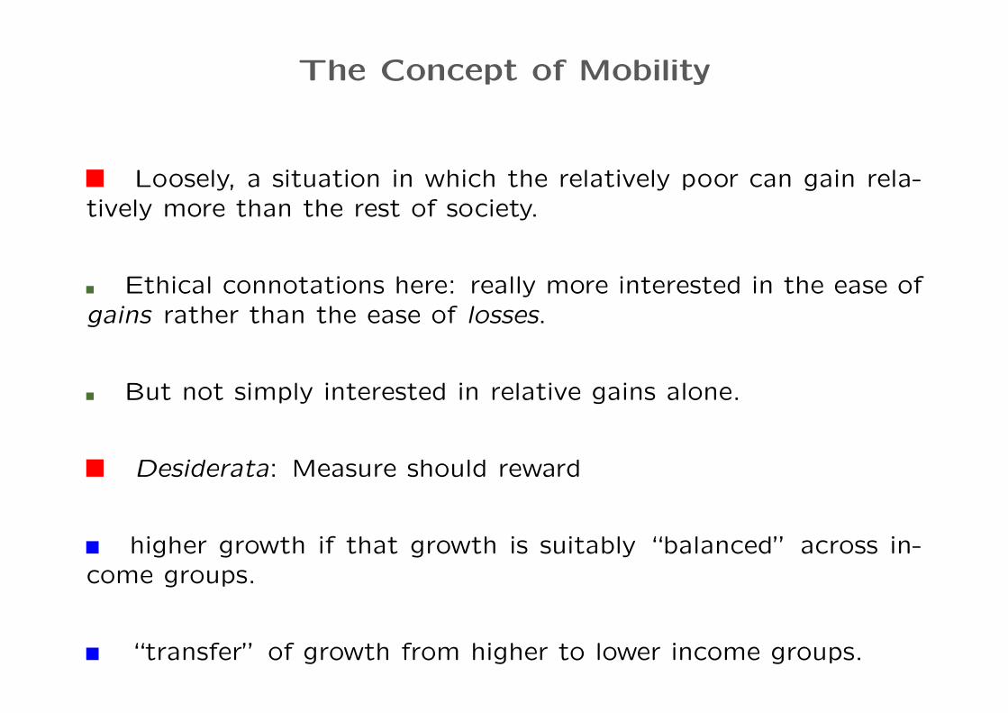
The Concept of Mobility

Loosely, a situation in which the relatively poor can gain rela-tively more than the rest of society.

Ethical connotations here: really more interested in the ease ofgains rather than the ease of losses.

But not simply interested in relative gains alone.

Desiderata: Measure should reward

higher growth if that growth is suitably “balanced” across in-come groups.

“transfer” of growth from higher to lower income groups.

0-2

Yet most mobility measures are relative:

Atkinson (1981), Bartholomew (1982), Chakravarty, Dutta andWeymark (1985), Conlisk (1974), Dardanoni (1993), Prais (1955),Shorrocks (1978).

Rewards “movement” in transition matrices whether this comesfrom growth or decline.

Many of these relativist measures also insensitive to who gains,the poor or the rich.

[But not all: see Benabou and Ok (2001), Chakravarty, Duttaand Weymark (1985), or Fields (2007).]

So the fundamental problem is that overall growth is ignored.

0-3

Fields and Ok (1996) and Mitra and Ok (1998) study absolutemobility.

Measures developed from coherent axiomatic basis.

But these papers have similar drawbacks:

Rewards change equally no matter from rich or poor.

Does not distinguish between upward and downward change.

At one level, easy to adjust these measures:

E.g., add a growth component to Chakravarty-Dutta-Weymark

Look at absolute Lorenz curves before and after (Silber andWeber (2005))

But extremely hard to evaluate: no axiomatic basis.

0-4

An Axiomatic Approach

Data: n individuals; for each i we have starting income yi andsubsequent growth rate gi.

zi = (yi, gi), and z = (z1, z2, . . . , zn).

A mobility measure is M defined on each z, continuous andanonymous.

Axioms:

[M.1] (Sensitivity to Growth) If gi ≥ g′i (strict inequality forsome i), then M(z) > M(z′).

[M.2] (Balanced Growth Normalization) If gi = g for all iunder z, then M(z) = g.

0-5

[M.3] (Sensitivity to the Poor) Suppose that yi < yj. Thena “growth rate transfer” from j to i raises mobility.

[M.4] (Independence of Irrelevant Alternatives) The growth-rate tradeoffs between any two persons depend only on the incomesand current growth rates of those two persons.

[M.5] (Relativity of Baseline Incomes) No mobility compar-isons are altered if every baseline income is scaled up by the samepercentage.

Proposition 1. A mobility measure satisfies [M.1]–[M.5] if andonly if it can be written as

Mα(z) =Pn

i=1 giy−αiPn

i=1 y−αi

for some α > 0.

0-6

Remarks on the Measure

Similarity to poverty-weighted growth rates (Chenery et al.(1974)) except that discipline imposed on income weights.

Power of characterization due to [M.3]:

[M.3] (Sensitivity to the Poor) Suppose that yi < yj. Thena “growth rate transfer” from j to i raises mobility.

makes sense as long there are no “income crossings”

But easy to extend to these cases (wait for the next draft!)

0-7

Mobility and Aspirations

We discuss aspirations as an important determinant of eco-nomic mobility.

Well aware of several important pathways:

poverty traps (Azariadis and Drazen (1990), Dasgupta and Ray(1986))

imperfect or missing credit markets (Banerjee and Newman(1993), Galor and Zeira (1993))

marital sorting (Fernandez and Rogerson (2001), Fernandez(2003))

The aspirations pathway is complementary to these.

0-8

Literature

Appadurai (2004) and Ray (2006) discuss the “capacity to as-pire”.

Karandikar et al. (1998) and Bendor et al. (2001) study aspi-rations in game theory.

Kahneman and Tversky (1979) and Kozsegi and Rabin (2007)study “reference points” in behavioral economics.

0-9

Aspirations: A Framework

Think of “aspirations” as some reference standard of living.

Aspirations gap: (relative) distance between aspiration and cur-rent standard of living.

Theory has two parts:

How individuals react to some given aspiration gap (positive ornegative).

The formation of aspirations.

Both these elements needed to close the model.

0-10

I. Reacting to Aspirations

Basic idea: large aspirations gap creates frustration, a small ornegative gap creates complacency.

Background Model

yt = ct + kt

yt+1 = (1 + r)kt

can add nonlinear production function, stochastic shocks . . .

Preferences: u(ct) + v(yt+1) + w(yt+1/at)

at is the aspiration of generation t (for next generation).

0-11

u(ct) + v(yt+1) + w(yt+1/at)

standard assumptions on u and v (logarithmic for calculations)

σt ≡ yt+1/at is the target gap (endogenous).

Assume utility excess (or shortfall) increasing at a decreasingrate in either direction.

0-12

z/a

w(z/a)

1

0-13

1− σ is the target gap (positive or negative).

Define γ ≡ yt/at (exogenous).

1− γ is the aspirations gap (positive or negative).

“Narrowing” or “widening” of the gap has obvious meanings.

An aspiration is unattained if target gap remains positive.

It is exceeded if the target gap is made negative.

0-14

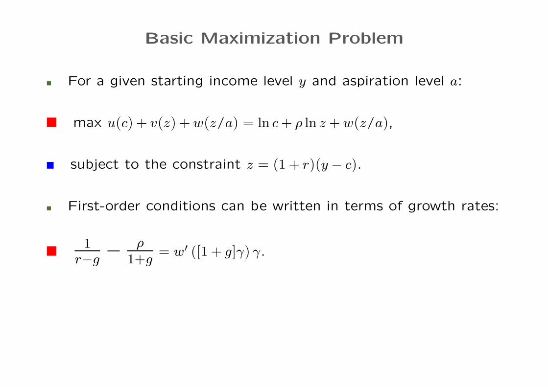
Basic Maximization Problem

For a given starting income level y and aspiration level a:

max u(c) + v(z) + w(z/a) = ln c + ρ ln z + w(z/a),

subject to the constraint z = (1 + r)(y− c).

First-order conditions can be written in terms of growth rates:

1r−g

− ρ1+g

= w′ ([1 + g]γ) γ.

0-15

g

LHS, RHS

rg1 g2

LHS

RHS

RHS

-1

0-16

Proposition 2. If aspirations are unattained, a narrowing of thegap must lead to an increase in growth.

If aspirations already exceeded the result is more complex.

Assume constant-elasticity: w(σ) = K1 + K2(σ− 1)b for σ ≥ 1.

Proposition 3. Suppose that b is not too high in the sense thatb(1 + r)γ < 1.

(i) If aspirations exceeded and gap is negative, a local narrowing ofthe gap must lead to an increase in growth.

(ii) If aspirations exceeded but gap is negative a local narrowing ofthe gap must lead to a decrease in growth.

0-17

2. The Determination of Aspirations

Internal or social? Social, in this talk.

Dependence on ambient environment in the form of incomedistribution.

Begin with simple case to illustrate:

at =Z

ydFt+1(y)

(where Ft+1 is next generation’s anticipated income distribution).

Individual with income y under Ft has aspiration γt(y) = y/at.

0-18

Equilibrium: a “consistent” sequence (Ft, at).

Steady State: incomes and aspirations grow at same rate g∗.

Equal Steady State: steady state with all incomes the same.

Necessary condition for equal steady state: g = g∗ must solve

1

r− g−

ρ

1 + g= w′

„1 + g

1 + g∗

«1

1 + g∗

Allows us to solve out for g∗:

1 + g∗

r− g∗− ρ = w′(1).

0-19

The Breakdown of Equality

Proposition 4. If w′(1) is steep enough while w is still bounded,an equal steady state cannot exist.

g

LHS, RHS

g*

LHS

RHS

g

LHS, RHS

g*

LHSRHS

g'

0-20

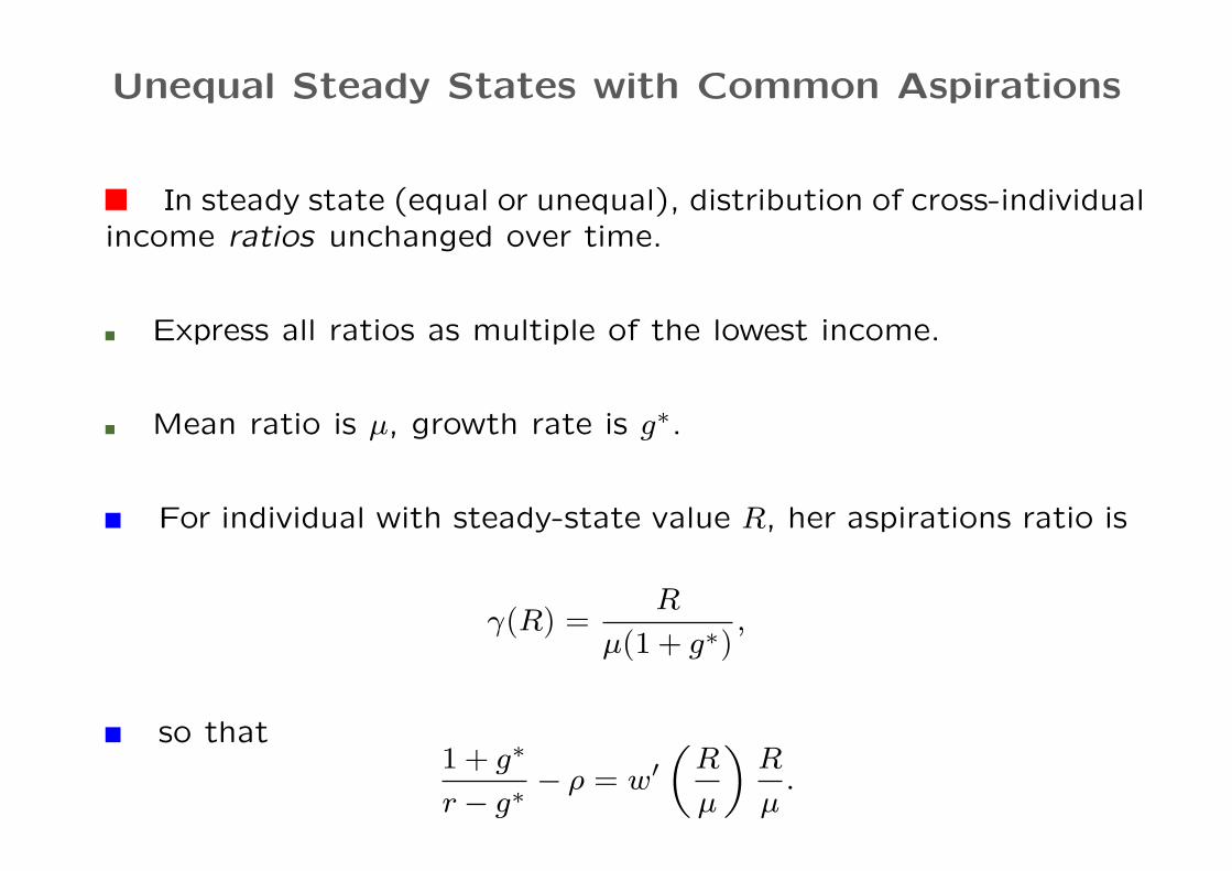
Unequal Steady States with Common Aspirations

In steady state (equal or unequal), distribution of cross-individualincome ratios unchanged over time.

Express all ratios as multiple of the lowest income.

Mean ratio is µ, growth rate is g∗.

For individual with steady-state value R, her aspirations ratio is

γ(R) =R

µ(1 + g∗),

so that1 + g∗

r− g∗− ρ = w′

„R

µ

«R

µ.

0-21

1 + g∗

r− g∗− ρ = w′

„R

µ

«R

µ.

Every unequal steady state with common aspirations must ex-hibit convergence to single mass point below the mean income ofsociety.

Convergence to one or more mass points above mean income.

E.g., if w′(σ)σ is declining in σ for σ > 1, just two mass points.

If w is constant-elasticity, no more than three mass points.

Equilibrium growth rates — and therefore mobility — mustdecline in steady-state inequality.

0-22

Looking Uphill: Diversity in Aspirations

We now depart from commonly held aspirations.

Natural formulation: individual looks at others richer than her.

Then

a(y) =1

1− F (y)

Z ∞

yxdF (x).

Corresponding aspirations ratio is γ(y) = y/a(y).

Assume earlier model plus symmetric constant-elasticity w(σ)with coefficient b; b(1 + r) < 1.

0-23

Questions

How do aspirations vary along the income distribution?

What about the growth rates of different income groups?

How does overall inequality affect growth and mobility?

Do steady state income distributions exist?

0-24

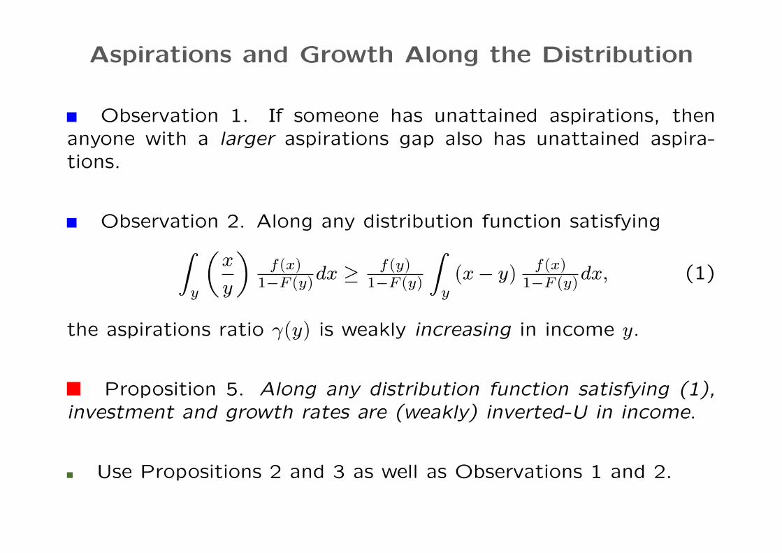
Aspirations and Growth Along the Distribution

Observation 1. If someone has unattained aspirations, thenanyone with a larger aspirations gap also has unattained aspira-tions.

Observation 2. Along any distribution function satisfyingZy

„x

y

«f (x)

1−F (y)dx ≥ f (y)1−F (y)

Zy

(x− y) f (x)1−F (y)dx, (1)

the aspirations ratio γ(y) is weakly increasing in income y.

Proposition 5. Along any distribution function satisfying (1),investment and growth rates are (weakly) inverted-U in income.

Use Propositions 2 and 3 as well as Observations 1 and 2.

0-25

Example : Uniform distribution over [a, b].

a = 1, 000, b = 100, 000, ρ = 0.9, r = 0.38, K1 = 0, K2 = 20, b = 0.5.

0 1 2 3 4 5 6 7 8 9 10

x 104

0

0.1

0.2

0.3

0.4

0.5

0.6

0.7

0.8

0.9

1

income y

0-26

0 1 2 3 4 5 6 7 8 9 10

x 105

-0.4

-0.2

0

0.2

0.4

0.6

0.8

1

y

growth ratesgammas

0-27

Overall aggregate growth rate is 32%.

But families along the distribution experience very differentrates.

Mobility significantly lower: M1 is 3% and M2 is −20%.

(remember mobility numbers normalized for comparison withgrowth)

0-28

Easy to see that γ(y) = 2yb+y

.

Increase in b raises inequality; lowers γ(y) for all y.

More inequality

Reduces growth rates for all unattained aspirations.

Increases growth rates for exceeded aspirations.

Net effect on growth is ambiguous.

(If b ↑ to 150,000, overall growth unaffected at 32%.)

0-29

0 1 2 3 4 5 6 7 8 9 10

x 105

-0.4

-0.2

0

0.2

0.4

0.6

0.8

1

y

growth ratesgammas

0-30

0 1 2 3 4 5 6 7 8 9 10

x 104

-0.4

-0.2

0

0.2

0.4

0.6

0.8

1

y

growth ratesgammasgrowth ratesgammas

0-31

Effect of higher inequality on mobility is clearer.

If b ↑ to 150,000, M1 falls to 0 and M2 to −24%.

0-32

Steady State Distributions

Which income distributions generate equal growth for all?

Pareto distribution with parameter κ > 1,

γ(y) =κ− 1

κfor all y.

Generates balanced growth.

Conjecture. Every steady state must belong to the class ofgeneralized Pareto distributions.

0-33

As before, can study growth-inequality tradeoff in steady state

(reduce κ to increase inequality).

Net effect depends on whether aspirations are attained to beginwith.

In a highly unequal society aspirations are unattained:

Greater equality results in higher growth.

But in highly equal societies, aspirations may be exceeded sothat a further reduction in inequality reduces growth.

0-34

0 0.1 0.2 0.3 0.4 0.5 0.6 0.7 0.8 0.9 1-0.4

-0.3

-0.2

-0.1

0

0.1

0.2

0.3

0.4

Gini Coefficient

Mob

ility

Mobility and Growth

0-35

Rough Sketch of a Numerical Application

Estimate parameters of lognormal approximation for incomedistributions in the US & some LA countries (late 1980s).

Find rates of return r to match predicted aggregate intergen-erational growth rates to actual growth over 15-year window

Forces predictions of growth rates by income categories in thesecountries.

Allows assessment of overall mobility

(variations possible once we have data on growth by incomecategories)

0-36

Estimating Lognormal parameters µ and σ:

One-to-one between σ and the Gini (Aitchison and Brown (1966)):

σ = 2(Φ−1((1 + G)/2))2.

Mean µ simply a function of σ and per-capita µy:

µ = ln µy −σ2

2.

Data:

Ginis from UNU-WIDER and

GDP pc in constant 2005 international $ (PPP) from WDI

0-37

The parameters:

Country GDPpc Gini µ σ

Brazil 89 7,692 0.63 7.61 1.64Costa Rica 86 5,520 0.46 8.33 0.75Mexico 89 8,900 0.46 8.81 0.75Chile 89 6,501 0.44 8.55 0.68Columbia 88 4,742 0.44 8.23 0.68Argentina 90 7,472 0.43 8.71 0.65US 89 31,640 0.38 10.24 0.50

0-38

Now let ρ = 0.9, r = 0.38, K1 = 0, K2 = 20 and b = 1/2 as before

Find returns to capital r that matches aggregate growth ratesover 15-year window:

Country r annual i Growth

US 89 0.3527 2.03% 0.2986Argentina 90 0.5110 2.79% 0.4473Brazil 89 0.2751 1.63% 0.0852Chile 89 0.8746 4.28% 0.8011Colombia 88 0.2492 1.49% 0.1594Costa Rica 86 0.4852 2.67% 0.4069Mexico 89 0.3410 0.25% 0.2572

Now generate growth rates by income category:

0-39

negative growth rates for the poor

Brazil vs. Argentina: similar income; higher inequality in Brazil

0-40

Mobility:

Country GDPpc Gini M1 M2 M5 Growth

US 89 31,640 0.38 0.26 0.23 0.14 0.30Arg 90 7,472 0.43 0.36 0.28 0.07 0.45Chi 89 6,501 0.44 0.72 0.64 0.44 0.80Col 88 4,742 0.44 0.07 0.00 −0.18 0.16Cos 86 5,520 0.46 0.27 0.16 −0.05 0.41Mex 89 8,900 0.46 0.13 0.01 −0.22 0.26Bra 89 7,692 0.63 −0.32 −0.39 −0.39 0.09

Compare mobility to growth.

Negative correlation between mobility and inequality.

0-41

Summary

Paper studies interconnections between mobility and aspira-tions.

Important to start with a tractable, axiomatically well-foundedmeasure of mobility.

Our mobility measure is indexed by a single parameter which weplan to restrict further in future work (discrete versus continuousgrowth paths).

We then turn to a model of aspirations that builds on theoryof reference points.

Main difference is that we “close” that model using socially-determined references or aspirations.

0-42

Summary, contd.

We embed aspirations into a model of growth.

Theory predicts how growth rates move on the income cross-section.

Theory also predicts a connection between rising inequality andlower mobility, though an ambiguous connection between inequalityand growth.

Finally, possible to study steady-state income distributions inwhich all income-specific growth rates are the same.

For these distributions the theory predicts a generally negativerelationship between inequality and growth.

0-43