IEEE TRANSACTIONS ON SYSTEMS, MAN, AND CYBERNETICS, V(5)0.. SMC-8. No. 7, Jiltly 1978

[7] J. N. Warfield, "Toward interpretation of complex structuralmodels," IEEE Trans. Syst., Man, Cybern., vol. SMC-4, pp. 405-417,Sept. 1973.

[8] D. V. Steward, "Partitioning and tearing systems of equations," J.SIAM Numer. Anal., ser. B, vol. 2, no. 2, pp. 345-365, 1965.

[9] R. D. Smith et al., "System partitioning study final report," McDon-nell Douglas, Rep. MDC G6603, Dec. 1976.

[10] R. J. Bidlack and C. R. Everhart, "System partitioning methodologyand evaluation," Teledyne Brown Engineering, Huntsville, AL,Interim Rep. SD76-BMDSC-2049, Oct. 1976.

[11] J. L. Uhrig, "A life-cycle evaluation model for system partitioning,"Bell Laboratories System Architectural Study Report to U.S. ArmyBMDSCOM, Huntsville, AL, Apr. 1977.

[12] A. D. Hall, III, "Three-dimensional morphology of systems engineer-ing," IEEE Trans. Syst. Sci. Cybern., vol. SSC-5, pp. 156-160, Apr.1969.

[13] J. N. Warfield, "Crossing theory and hierarchy mapping," IEEETrans. Syst., Man, Cybern., vol. SMC-7, pp. 505-523, July 1977.

[14] G. B. Dantzig, Linear Programming and Extensions. Princeton, NJ:Princeton Univ., 1963.

[15] T. C. Koopmans and M. Beckman, "Assignment problems and thelocation of economic activities," Econometrica, vol. 25, pp. 53-76,Jan. 1957.

[16] A. H. Land, "A problem of assignment with inter-related costs," Opnl.Res. Quart., vol. 14, pp. 185-199, June 1963.

[17] L. Steinberg, "The backboard wiring problem: A placement algo-

rithm," SIAM Rev., vol. 3, pp. 37-50, Jan. 1961.[18] R. J. Freeman et al., "A mathematical model of supply support for

space operations," Oper. Res., vol. 14, no. 1, pp. 1 -15. Jan. -Feb. 1966.[19] R. C. Carlson and G. L. Nemhauser, "Scheduling to minimize inter-

action cost," Oper. Res., vol. 14, no. 1, pp. 52 -58, Jan.-Feb., 1966.[20] H. Greenberg, "A quadratic assignment problem without column

constraints," Naval Res. Logist. Qiuart., vol. 16. no. 3, pp. 417 421,Sept. 1969.

[21] L. J. Ackerman et al., "Application of sequencing policies to tele-phone switching facilities," IEEE Trans. Svst.. Mlan. Cybern. vol.SMC-7, pp. 604-609, Aug. 1977.

[22] E. L. Lawler, "The quadratic assignment problem," Management Sti.,vol. 9, pp. 586-599, July 1963.

[23] G. Hadley, Nonlinear and Dynamic Programming. Reading, MA:Addison-Wesley, 1964.

[24] G. H. Hardy et al., Inequalities, 2nd ed. Cambridge, England: Cam-bridge Univ., 1964.

[25] J. L. Uhrig, "Life-cycle evaluation of system partitioning," in Proc.Ist Int. Computer Software and Applications Conf, Chicago, IL. Nov.1977.

[26] A. P. Sage, "On interpretive structural models for single-sink digraphtrees," in Proc. Conf Systems, Man, and Cybernetics, Washington,DC, Sept. 1977.

[27] A. P. Sage and T. J. Smith, "On group assessment of utility and worthattributes using interpretive structural modeling," Compuiters alndElec. Eng.. vol. 4, no. 3, pp. 185-198. Sept. 1977.

Correspondence-

Determining Compatibility Coefficients forCurve Enhancement Relaxation Processes

SHMUEL PELEG AND AZRIEL ROSENFELD, FELLOW, IEEE

Abstract Relaxation labeling is a process that attempts todisambiguate probabilistic labelings of objects. Compatibilitycoefficients play an important role in the relaxation process. Noexplanation exists at present for their exact meaning, and noalgorithm has been proposed to generate them. Some possibleinterpretations of these coefficients are presented, and algorithms aresuggested to obtain them from the initial probabilistic labeling.Examples are given for the case where relaxation is used todisambiguate the detection of curves in a picture.

I. INTRODUCTION

In many image processing tasks a classification of each pointinto one of several classes is desired. For example, in line detec-tion, points are classified as being on a line having a certain direc-tion or as not being on a line. However, classification processessuch as this, based on local detection, do not usually give perfectresults. The processes are sensitive to local noise and sometimescannot determine the exact classification. A line detector, for

Manuscript received October 7, 1977; revised February 6, 1978. This work was

supported in part by the National Science Foundation under Grant MCS-76-23763.S. Peleg's studies were supported by the Lady Davis Fellowship Trust.The authors are with the Computer Saence Center. University of Maryland, Col-

lege Park MD 20742.

example, can often find substantial responses in several directionsat a given point. A method that has been used to improve theinitial classification is relaxation labeling.To apply relaxation labeling, we initially assign to each point

the probabilities of its possible class memberships, based on localinformation. The relaxation labeling process uses knowledge ofhow labels interact locally to improve and disambiguate this priorclassification. This process is described in Section 11. This corre-

spondence suggests several automatic methods of determining themutual support coefficients used in relaxation according to differ-ent possible interpretations of these coefficients.

II. THE RELAXATION LABELING PROCESS

In this section we review some of the concepts involved in

relaxation labeling. The subject is discussed in greater detail in

[1]; for further references see [2].The relaxation process involves a set of objects A - a I, a2,

an} and a set of labels (class names) A = {A', A2, *m} For eachobject a, we are given a set of local measurements, which are usedas a basis for estimating the probabilities Pi(A) of object at havingeach label i. These probabilities satisfy the condition

(1)Z Pi(A)= 1. for all ai E AI 0 < P,(s.) c 1.A E A

The relaxation process is a parallel algorithm that updates theprobabilities of labels. The probabilities are updated using a set of

0018-9472 78/0700-0548$00.75 CO 1978.IEEE

548

CORRESPONDENCE

(a) (b) (c) %%AI

Fig. 1. Images used in experiments. (a), (b) Original images. (c), (d) Edge detector outputs.

given "compatibility coefficients" r1AA, A'), where rnj: A x A[-1, 1] and:

a) if A and A' are compatible for objects a, and aj, respectively,then rij(A, A') > 0;

b) if A and A' are incompatible for a, and aj, respectively, thenr1j(A,A') < 0;

c) if neither labeling is constrained by the other, then rgj(A,A') = O;

d) the magnitude of r,j represents the strength of thecompatibility.

Methods for computing the r,j are suggested in Sections IV and V.We now discuss the probability updating rule. The updating

factor for the estimate P,k(A) (at the kth iteration) is

q$(A) = 1 E rij(A, A')Pj(A') (2)

where n is the number of objects. The new estimate of the probabi-Lity of A at a, is

k++l)(A) Pi'(AXI + qt1(A)], P; (A')[1 + qk'(A')](

Thus each Pil(A) is multipLed by [1 - qi(A)], and the values are

normaLized at each object to satisfy (1) The relaxation process isiterated until some termination criterion is met.

III. CURVE ENHANCEMENT USING RELAXATION

Since the domain from which the examples in this report are

drawn is curve enhancement, this application is briefly describedin this section. A detailed discussion appears in [3]. Line detectorsare applied to the picture, and at each point probabiLities are

assigned to nine labels: Lines in eight possible directions and a "noLine" label.Two methods of line detection can be used: Linear and nonlin-

ear. The response of a Linear line detector for vertical Lines, giventhe configuration of points

a b c

d e fg h i

will be 2(b + e + h) - (a + c + d +f+ g + i). The response of a

nonlinear detector for vertical Lnes will be

2(b + e + h) - (a + c + d +f+ g +i),

if a<b>c, d <e>f, g<h>i

0,

otherwise.

The initial probabilistic labeling is obtained from the line detectoroutput by normalization (see [3])The coefficients used in the probability updating rule will be

discussed below. They are computed only for neighboring pairs ofpoints; in other words, they are assumed to be zero for nonneigh-boring point pairs.

The following simplifications have been made in the relaxationprocess described in Section II. The probability of a label whosecurrent estimate is greater than 0.9 and which gets maximumsupport is increased to 1, and that point is never considered againfor updating. Also, the q1(A) of (2) are not divided by n (when thisdoes not violate the condition q(A) > - 1), in order to increasethe effect of each iteration on the P,(A)

Input images for our curve enhancement experiments were ob-tained by applying an edge detection operator (based on differ-ences of two-by-two averages) to the two pictures shown in Fig.1(a), (b), yielding the outline pictures shown in Fig. 1(c), (d}

IV. CoMPATIBILrry COEFFICIENTS AS CORRELATIONSFor brevity, let p,j denote the compatibility between the points

(x, y) and (x + i, y +j)-e.g., pIo(A, A') is the compatibility be-tween label A at a point and label A' at its right-hand neighbor.One possible interpretation of the compatibilities is in terms of

statistical correlation, since correlation has properties a)d) listedin Section II. Estimates of the correlation coefficients derived fromanalyzing the initial labeling are

E [P(x,,)(A) -(A)J[P(X+I,,+,,(A')-P(A')]Rij(A, A') = (x,y) a(A)a(A') (4)

Here P(.,b)(A) is the initial estimate of the probability of labelingpoint (a, b) with A, P(A) is the average of P(X,,)(A) for all points (x,y), and a(A) is the standard deviation of P(X, )(A)To test these R,J in a line enhancement relaxation process, non-

linear line detection operators (see Section III) in eight orienta-tions were applied to the picture in Fig. 1(c), and the responsestrengths were used, as in [3], to compute initial estimates of theprobabilities of the nine labels (eight line orientations and "noline"> Fig. 2(a) is a symbolic representation of the most probablelabel at each point; the "no line" labels are represented by solid3 x 3 squares with gray level proportional to the "no line" prob-ability (0 = black, 1 = white), while the line labels are representedby three-point line segments in the appropriate orientations withgray levels "negatively proportional" to the line probability(0 = white, 1 = black}, It can be seen that the line detections aresomewhat noisy.Table I shows correlation coefficients derived from Fig. 2(a)

using (4), and Fig. 2(b)-(d) show iterations 2, 6, and 12 of therelaxation process using these coefficients, appLied to Fig. 2(a)The results are very poor. This is because when one label domin-ates the picture, as the "no line" label does in our case, its correla-tion coefficients with all other labels are high. Thus in therelaxation updating, the "no line" label gets most of the support,and after a few iterations almost all the points have this labeL ,The effect of dominance among labels can be alleviated by

weighting the R's by the probabilities that the corresponding labelsdo not occur. This greatly reduces the values of the coefficientsinvolving dominant labels, but will only slightly reduce the valuesof the coefficients involving rare labels. The new coefficients are

Rt(A, A') = [1 - P(A)][l - P(A')] RiJ(A, A') (5)

549

IEEE TRANSACTIONS ON SYSTEMS, MAN, AND CYBERNETICS, VOL. sMC-8, NO. 7, JULY 1978

(b)(a)

(c) (d)

Fig 2. Iterations 0, 2, 6, 12 of relaxation proces using unweighted correlationcoefficents derived from Fig. 2(a) (For explanation of symbols in these figures, seetext.)

TABLE ICORRELATION COEFFICIENTS DERIVED FROM FIG. 2(a)

0o16 -019 0 03 0 04 0 -0 07 -0.06 -010 -0 02-012 0.26 -0. 02 -0. 02 -0 01 -0 03 -0. 0 0.01 -0. 020.03 -0-02 0.00 -0.01 0~00 -0.02 -0.01 -0.01 -0.01

a) 0.04 -0.02 -0.01 -02 0.02 -0.02 -001I -0.01 -0 01a) ~ 0.0 -0.01 -00 -001l -002 -00I0.1-0-0:09 -003 -00 -002 -0~02 0,21 0-0 -0.0-0.03 0 01 -001 - 001 0.03 -001 019og -&000 -.001-06 -01 -0.01 -0.01 -0.01 0.00 -0.00 0. 43 -0.01

-0 is 0~19 -0.01 -0 01-01-02-.1 0.1 0 16

0 49 -0. 50 -0. 09 -0. 09 -0.01 -0 09 -0 04 -0. 01 -0. 20-0.53 0.83 0.03 -_002 -0.02 -0.03 -0.01 -0.01 0.13-0.16 0.10 0.32 0.07 -0.00 -0.02 -0.01 0.01 0.00-0.08 -0.02 -0.01 29 0.05 -0.02 -0.01 -0.01 0.02b) 0 02 -0.02 -0.01 -0 01 003 -0 02 -e 01 -0o01 -0o01-0. 11 -003 -0.01 -0.02 -0. 02 025 0.0 -00 -002-0. 03 -0. 01 0.00 0.02 00 7 -0 01 13 -0.00 -001-0 06 -0 01 -0. 01 -0 01 -0. 01 0.00 -0.00 0. 19 0 13-0 08 -002 0.00 -0.01 -0,01 -0.02 -0.01 -001 O:35

0 29 -0.13 -0.14 -0.25 -0.13 -0.11 -0.01 0.02 -0.03-019 0.27 008 -0 02 -0 02 -0.03 -0.02 -0.01 0.08-0 04 -_002 0.21 00 7 -0.00 -0.02 -0.01 -0.01 -0.01-0 25 -0.02 0.11 0 78 O003 -0.02 -0.01 -0.01 -0.01

-0 06 -0. 00 -0.01 002 029 -0 02 -0.01 -0.01 -0.01-0 15 -003 -0.02 -0 02 0 11 0 28 0.06 -0.01 -0.02-0.00 -0. 00 0.00 0.02 -0.00 0 01 -0.01 -0.00 -0.010.01 -0 01 0.03 -0 -0 01 -0 01 -0 00 -0 00 -0 010.01 -0.02 0.04 0. 01 -001 - 002 - 001 -0.01 0 00

where Rjj is defined by (4)1 These coefficients have the propertythat they support rare labels at points having no evidence fromtheir neighborhoods, since the self-support coefficients (the Roo)are the highest for the rare labels. In case this effect is undesirable,one might ignore the self-support in the relaxation.The coefficients defined by (5) for the case of Fig. 2(a) are shown

in Table II. Fig. 3 shows iterations 0, 2, 6, and 12 of the relaxationprocess using these coefficients, and Fig. 4 is analogous exceptthat the self-support coefficients are ignored. (Figs. 3(a) and 4(a)are the same as Fig. 2(a)) The results are extremely similar andare much better than those in Fig. 2. The ambiguity has beengreatly reduced, and the curves have survived the process. Notethat the surviving curve points are, for the most part, just thepoints whose most probable initial label was a line label; theresults do not differ greatly from a maximum-likelihoodclassification of the points based on the initial probabilityestimates.

It should be noted that the ideal correlation coefficients shouldbe symmetric, i.e., pairs of neighbors on opposite sides of a pointshould yield the same sets of coefficients (transposed) In theestimated coefficients of Tables I and II, this is almost exactly true.Any discrepancy is due partly to computational error and partlyto picture border effects. Analogous remarks apply to the tables ofmutual information coefficients (Table III, ff.)

V. COMPATIBILITY COEFFICIENTS AS

"MUTUAL INFORMATION"A different approach to defining compatibility coefficients is

based on the mutual information of the labels at neighboringpoints. This approach too satisfies our intuitive ideas about thenature of the coefficients: If two labels have a high positivecorrelation, we can expect them to have a high mutual informa-tion, and vice versa.We estimate the probability of any point having the label A by

PF(A= 1 E P)(,y)

(6)

The choice of weighting function in (5) was somewhat arbitrary. For example, we

could have chosen to define the weight to be /[1 P(A)][1 P(A')] rather than[I P(A)][I P(AX)], i.e., the geometric mean rather than the product.

0.40 -0.17 0.02 -0.06 -o.013 -0:43 -0 04 -007 0o00-0.12 0o26 -0 02 -O 02 -0.02 -0 03 -0 -0. 01 -0 02-002 -002 -006 -001 0.01 -0.02 -0:01 -0.01-0g06 -0 02 -0.1 0g29 0g00 -0g02 -0g01 -0.010g082-0.09 -0 02 -.01 -.0 0.36 0.05 -0.01 -01 -0.01

42 -003 -.02 -0.02 0.10 0.81 -00 :-01-010 -002 -001 003 00 010 036 -0.00 -00101 -0 01 -0 01 -O 01 -001 0 00 -0 00 05 -001

-0. 11 0 15 -0 01 -0 01 -0 01 -0 02 -0 01 0 25 -0 01

0.99 -0 58 -.26 -29 -026 -0.51 -0.14 -0.14 -0.29-0:58 0:99 002 -0.092 -0.02 -03-001 -0.01 -0.02

-0 26 0 2 1.0 0.03 -0.00 02 1 -001e) -0 29 -0 02 0 03 1 00 0 00 -0 02 -0 01 -0 01 0 0

-0.26 -0 02 -0.00 0.00 100 0.04 -0 01 -0.01_001-_0 51 -0 03 -0g02 -0.02 004 1°00 -0.01 -0 01 -0 02

-0 14 -0 01 -0. 01 -001 -0. 01 -0. I 00 -0 00 -0 01

-0 14 -0.01 -0.01 -0.01 -0.01 -0.00 1.00 -0 0

-0:29 -002 -001 -0g01 -001 -002 -0.01 -0.01 100

0:41 -0: 12 -0 02 -0.06 -009 -0 44 -010 0:01-017 026 -002 -00 2 -0 02 -003 -002 -001 0150.02 -0 02 0.06 -.01 -001 -0 02 -001 -o0 -0. 01-0 .06 -001 0.29 -0 01 -0f ) - 16 Jg: 02 0g0lg:008:3 g 1o83 0g: 01~gg13 02 0.01 00 0 36 0 10 -0 01 -0 01 -0.01

-0.45 -0 03 -0.02 -0o02 0.05 _0985 0. 10 0.00 -002-0.04 -001 -0~01 -0~01 -0.01 -001 036 -O000 -0 01

-0g07 -0 0l -0 0l -001 -00l -_0,01 -0:00 0g05 0 250o00 -0.02 0.08 002 -0 01 -0.02 -0 01 -0.01 -0.01

0 29 -0.1 -0 04 -0.25 -0.06 -0o14 -0.00 0.01 0.01-0.13 027 -0 02 -002 -0.00 -0 03 -0.00 -0.01 -0.02-0214 0.08 02 0.11 -0 01-0g02 0g00 0.03 0.04

-0.25 -0.02 0-07 07 002 -002 002 -0 01 0 01

g -013 -002 _0.00 0.03 0229 0 -000 -g00 -0-0.109 0.03 002 -0.02 -O 02 0. 0.01 -001 -0 02-0.01 -0 02 -001 -00 -00 0.06 -00 -000 -0.01002 -0.01 -001 -001 -001-'001 -000 -000 -0.01

-0.03 008 001 -0.01 -o001 -002 -0 01 -0 01 0 00

0o4 -0o52 -0. -0.08 0.02 -0911 -0o03 -0.06 -00-0 49 0 2 0.0 -0.002 -02 -003 -0.01 -0.01 -0.02

: g43 :0.030g32 -00 2 0.00 -01 0 00

-0 .01 -0.02 0.02 -0.

h) 0.02001-0 00 O.02- . 03 -0. 02 _0.07 -0.01 -0.01o-00 -0 03 -0 02 -g02 -g02 025 -001 -02

-0:049 -0.001 -0:1 -001 -001 0 06 0.13 -0 00 -0011-0 01 -001 001 -001 -001 -001 -0. 00 019 -0. 1

-0 20 0 130 00 -0 02 -0. 01 -0. 02 -0 01 0. 13 03

-0116 -0:12 _003 -004 0.03 -0.09 -0.03 -0 06 -019

025 -002 -002 -02 -0:03 0.01 -0.01 0:19003 .0 01_ 0 0 - 0 - 0

0 04 -0.02 -0 01 -00 -001 -0 -001 -0 001 -000

2 -001 00-002 -.1 -0 02 -003 -0.01 -001

il -~0 0.01 0:0 -0.0

-000 -.0 -001 -0~01 009 019 -000 -0.01

-0.10 -0.0 001 -0 .0001-00

0 -0 -0.01 -0 00 0 403 .0

-002 -0 02 -0.01 -0.01 -0.01 -0.02 -0.01 -0.01 0. 16,

The nine parts (a-i) correspond to the nineneighbors of point (e) in the following order:

a b cd e fg h i

In each part, the first row and first columncorrespond to no-line probabilities; the remain-ing rows and columns correspond to slopes measuredclockwise from the vertical in steps of 221°F'

550

CORRESPONDENCE

(b)

(d)

ig, 3. Analogous to Fig. 2, but using weighted correlation coefficients.

(b)

(d)

Fig. 4. Same as Fig. 3. but ignoring the self-support coefficients.

TABLE IIWEIGHTED CORRELATION COEFFICIENTS DERIVED FROM FIG. 2(a)

0. 00 -0.01 -0. o0 0.o0 o 00 -o00 -0.00 -0.01 -0. 00-0.01 0. 25 -0. 02 -0. 02 -001 -O 03 -.00 -0. 01 -0 02

a) Q O2 O.000-0.01 000 -O 2 -O 01 -0.01 -0 01a, O. 00-O. 02 -O. 01 - 002 O 02 -O 2 -0 01 -0. 01 -0 01O 00 -0 01 -. 01 -0 01 -0 1 - 2 -o.00 -o.00 -0 01

-0.01 -0. 03 -0. 01 -0.02 -002O 20 0.08 -0.01 -002-0. 00 0 01 -0 01 -0.01 0 03 -O 01 0 19 -0 00 -0 01-O 00 -0.01 -0.01 -O 01 -O 01 0 00-000 0.42 -001-001 0.19 -0.01 -0.01 -0 01 -02 -01. 01. 0O 16

0.00 -0.03 -0.01 -0.01 -000 -001 -0.00 -0O00 -0.01-0.04 0.79 0.03 -0.02 -0.02 -003 -0.01 -0.01 0.12-001 0.10 0.32 0.07 -0.00 -0.02 -0.01 0.01 0.00

b) -0. 01 -0.02 -0.01 0.29 0. 05 -0.02 -0.01 -0. 01 0.020. 00 -0.02 -O 01 -O. 01 0.03 -0.02 -0.01 -0. 01 -0.01-0 01 -0.03 -0.01 -0.02 -0.02 0.24 O.06 -0.01 -0.02-0.00 -0.01 0.00 0 02 07 -001 13 -0.00 -0.01-0 00 -001 - 01 -O.01 -.01 00 -. 00 0. 19 013-0.01 -002 0 00 -0.01 -0.01 -002O -0 01 -0. 01 0 34

000 -O 001 -0 01 -0.02 -0.01 -0.01 -0000 00 -0.00-0 01 0.26 0.08 -0.02 -0.02 -0.03 -0.02 -0.01 0.08-0.00 02 0.21 00 -000 -0.02 -001 -0.01 -.01

cl -°0.02 -.02 0. 10 0 76 003 -0o02 _0.01 -0. 01 -0 01-O.00 -0.00 -0.01 0.020o29 -002 -01 -0.01 0-.01-0.01 -0.03 -0.02 -O 02o 11 0.27 0. 0 -0 0 -0 02-0. 00 -0.00 0.00 0.02 -O. 00 0.00 -0. Ol -O. 00 -0. 1

0. 00 -0.01 0.03 -0.01 -0.01 -0.01 -0.00 -0.00 -0.010 00 -002 0.04 001 -001 -0.02 -0.01 -0.01 000

0.00 -0.01O 0 00 -0.00 -0.01 -0.03 -0.00 -0 01 000-0.01 0.25 -002 -0.02 -0.02 -0.03 -001 -O01O -0.02-0. 00 -0.02 006 -0 01 0.01 -0.02 -0.01 -O 01 008-O000--0.02 -001 029 0 00 -0.02 -0.01 -0. 01 002

d) °-001 -0.02 -0.01 -O 01 0 35 0.04 -0.01 -0.01 -0.01-0.03 -0.03 -0 02 -002 0.09 0.79 -0.01 -0.01 -0.02-0.01 -2 -001 003 -0. 1 10 0 36 -000 -0.01O. 00 -0O0 -I001 -0O01 -001 00 -0.00 0.05 -0.01

-0.01 0.14 -0.01 -0 01 -0.01 -002 -001 025 -0.01

0.00 -0.04 -0.02 -0 02 -0.02-0 04 0 94 0.02 -02 -0 02-0.02 0.02 0.99 03 00

e-)-002 -0 02 0 03 0o98 000

-0. 02 -0. 02 -0.00 00 0 99

-0.03 -0 03 -0. 02 -0 02 0 03-001 -0 01 -0.01 -_001 -0 01-0.01 -0 01 -0.01 -0.01 -001-0.02 -0.02 -0.01 -0.01 -0.01

-0 03-0 03-0 02

-0 020 030 96

-0 01

-0 02

-0 01 -0 01 -0 02-001 -001 -002

-0 -0. -001-0. -0 01 -0 01-0.01 -0.01 -0 01

-0.01 -0 -0 -0 020 99 -0 00 -0 01

-0 00 1 00 -O 01-0.01 -001 0 99

0.00 -0.01 -0.00 -0.00 -0 01 -0.03 -0.01 0.00 -0.01-001 0.25 -0.02 -0 02 -002 -0.03 -0.02 -0.01 0.140.00 -0.02O 0.06 -0.01 -0 01 -002 -0.01 -0.01 -0.01-0 00 0.02 0. 01 0.28 0 01 -0.02 003 -0.01 -0.01

f) -0.01 -0.02 0.01 0.00 0.35 0.09 -0.01 -0.01 -0.01-0.03 -0.03 -0.02 -0.02 0.04 0.02 0.10 0.00 -0.02-0 00 -0 01 -. 01 -0.01 -0 01 01 .36 -0 00 -0. 010. 01 001 -0. 01 -0. 01 -001 -001 -0.00 005 025000 -002 00 00 -0.01 -0.02 -001 -001 -0.01

0 00 -0 01 -0.00 -0.02 -0 00 001 0 00 0. 00 0. 00-0.01 0.26 -0 02 -0.02 -00 -003 -000 -001 -0020 01 0 08 021 010 001 -02 0 00 0 03 0 04-0.02 -0.02 0.06 -0O002 02 -0 01 0.01

g) -0°01 -0.02O 0 00 0 03 0 29 0. 11 -0.00 -0.01 -0.01-0.01 -003 -002 02 -002 0 28 0 00 -0 01 -0.02-0.00 -0 02 -0.01 -0.01 0.01 006 001 -000 -0 010.00 -0 01 -0.01 -0.01 -0.01 -0.01 -0. 00 -0 00 -01-0.00 0.08 -0.01 -0.01 -0.01 -0.02 -001 -001 0.00

and the joint probability of a pair of points having labels A and A'by

PipA, A') E (7)n (,.y)

where n is the number of points and P(,y)(A) is the initial estimateof the probability of point (x, y) having the label A. We can now

estimate the conditional probability that (x, y) is labeled A giventhat (x + i, y + j) is labeled A' by

P IAl (8)P(A') (i)(xX(a.y)

For any event A whose probability of occurrence is P(A), theamount of information we receive as a result of being told that Ahas occurred is defined by

I(A)= -log P(A). (9)This information is zero when P(A) = 1, since we knew alreadythat A will occur, and approaches infinity when P(A) approacheszero. In the same manner, the conditional information that we

0.00 -0.04 -0.01 -0.01 0.00 -0o01 -0.00 -0.00 -0.01-0.03 0.78 0 10 -. 02 -0 02 -0 03 -0 01 -0 o -0. 02-0.01 0.03 0.32 -O 01 -001 -0:01 0.OO -0.01 0.00-0.01 -0.02 0.07 0.29 -0.01 -0. 02 0. 02 -0.0 -0. 01,O 00 -0.02 -0.00 0. 05 0.03 -0. 02 00 7 -0 01 -0. ol-0. 01 -0.03 -0.02 -0.02 -0.02 0. 24 -0.010l00 -0. 02-0 00 -0.01 -001 -001 -0.01 0.08 0.13 -00. 0 -0. O

-0 00 -o 01 ol0 -0.01 -ol -O 01 -0. 00 0 19 -0.01-0 01 0 12 0.00 0 02 -0 01 -0.02 -0.01 0 13 0.34

000 -0 01 O0 00 O0.00 0 00 -001 -000 -0.00 -001-0 01 0 24 -0 02 -0. 02 -o 01 -0 03 0 01 -0.01 0 19

0. 0 -0.02 0.00 -0.01 -0o01 -0 01 -0.01 -0.01 -0.010 00 -002 -0.01 -0.02 -0.01 -0o02 -0.01 -0.01 -0010.00 -0.01 0.00 0.02 -0.0 -0 02 0.03 -o001 -0.01

i) -0.01 -0.03 -0. 02 -02 -0.02 0. 21 -0.01 0.00 -02-0.00 -0.00 -0. 01 -0.0 -0 0.19 -0.00 -001-001 -0.01 -0

O-001 -00 -0 O -000 0.42 0 15

-0.00 -0.02 -00.o -0.01 -001 -0o02 -0.01 -0.01 0,16

receive if we already know that B has occurred and are told that Ahas occurred is

I(AIB)= -log P(A I B (10)

The contribution of B to the information about A is expressed bythe mutual information

I(A; B) = I(A) - I(A B) = log P(A B) (11)

Note that if A is highly correlated with B, P(A B) should be closeto one, so that I(A B) is close to zero, making l(A; B) high (close

(a)

(c)

Fi

(a)

(c)

551

IEEE TRANSACTIONS ON SYSTEMS, MAN, AND CYBERNEnCS, VOL. smc-8, No. 7, JULY 1978

TABLE IIIMUTUAL INFORMATION COEFFICENTS DERIVED FROM FIG. 2(a)

0.00 -0.05 0.01 0.01 0.01 -0.02 -0.03 -0.09 -0.01-0.03 _043 -1.00-°l: 00 -0.32 -0.85 -0.06 -1.00 -1.000.01 -1.00 _008 -1 00 0 01 -1 00 -1.00 -1.00 -1.00

a) B1 -.00 -100 1.00 0.17 -1.00 -1,0-I8 1.00 -1. 00a . 0 -0. 35 -1. 00 -1. 00 -1. 00 -1.0 -1. 00 -. 00 -. 00-0.02 -0.61 -0.21 -0.29 -1.00 0.40 O. 36 -1. 00 -1. 00-0. 01 0. -1. 00 -.00 0. 30 -1.00 -1.00 -.00-0.05 -1.00 -.00 -1.00 -1.00 0.07 -1.00 0.9 -1. 00-0.06 0.47 -1.00 -1.00 -1.00 -1.00 1.00 0.65 0.53

0.00 -0. 1 -0.04 -0.03 -0.00 -0.02 -0.02 -0.01 -0. 10-0.18 0.84 0.18 -1.00 -0.44 -0.74 -0.42 -100 0.39-0.07 0.36 0.69 0.37 -0.09 -1.00 -1.00 0.22 0.02-0 03 -1.00 -0.15 0.80 0.32 -1.00 -1.00 -1.00 0.15b) 0.01 -0.71 -1.00 -1.00 0.29 -1O00 -1.00 -1.00 -042-0.03 -0.52 -0.23 -1.00 -1.00 0.44 0.34 -1.00 -1.00-0.02 -0.23 0.09 0.19 0.44 -0.09 0.59 -1.00 -1.000-005 -1.00 -1.00 -1.00 -1.00 0.04 -1.00 0.82 0.82-0.03 -1.00 0.08 -1.00 -1.00 -1.00 -1.00 -1.00 0.88

0.00 -0.03 -0.07 -0.10 -0.06 -0.03 -0.01 0.01 -0.01-0.05 0.44 0.33 -1.00 -1.00 -0.49 -1.00 -1.00 0.32-0.02 -1.00 0.60 0.38 -0,07 -1.00 -1.00 -1.00 -1 00-0.10 -1.00 0.44 0.78 0.28 -1.00 -1.00 -1.00 -1.00

c) -0.03 -0.00 -0.23 0.21 0.89 -1.00 -1.00 -1.00 -1.0000-04 -0.53 -0.48 -1.00 0.39 0.48 0.32 -1o00 -1.00-0.00 -0.08 0.01 0.23 -0.10 0.08 -1.00 -1.00 -1.000. 01 -1. 00 0.39 -1. 00 -1. 00 -1. 00 -1.00 -1.00 -1. 000.01 -1.00 0.29 0.10 -0.14 -1.00 -1.00 -1.00 0.08

0. 00 -0. 04 0. 01 -0.02 -0. 08 -0. 14 -0. 02 -O. 06 0 00-0.03 0.43 -1.00 -1.00 -0.49 -0.90 -0.09 -1. 00 -1. 00-0.01 -1.00 0.38 -1.00 0. 14 -0.82 -1.00 -1.00 0.42-0.02 -1.00 -1.00 0.59 0.02 -1.00 -1.00 -1.00 0.18-0.04 -1.00 -1.00 -1.00 0.73 0.28 -0.39 -1.00 -027-0.13 -0.73 -0.46 -1.00 0.38 0.86 -1.00 -1.00 -1.00-0.08 -1.00 -1.00 0.25 -1.00 0.41 0.79 -1.00 -1.000.00 -1.00 -1.00 -1.00 -1.00 0.01 -1.00 0.58 -1.00-0.04 0.42 -1.00 -1.00 -0.17 -1.00 -1.00 0.75 -019

0.01 -0.21 -0.15 -0.13 -0.16 -0.18 -0.08 -014 -016-0.21 0.68 0. 16 -1.00 -0.51 -0.99 -0.43 -1 00 -1 00-0. 15 0. 16 0. 91 0.26 -0.08 -0.71 -1. 00 -1.00 -1.00

e) -0.13 -1.00 0. 28 0.83 0. 01 -1. 00 -1.00 -100 -1.00-0.18 -0.51 -0.08 0.01 0.93 0.22 -0.40 -1o00 -0.23-0.18 -0.99 -0.71 -1.00 0.22 0.70 -1.00 -1.00 -100-0.08 -0.43 -1.00 -1.00 -0.40 -1.000o99 -1.00 -I 00-0.14 -1.00 -1.00 -1.00 -1. 00 -1. 00 -1. 00 1.00 -1.00-0. 18 -1. 00 -1.00 -1. 00 -0.23 -1.00 -1. 00 -1.00 .e88

0.00 -0.03 -0.01 -0.02 -0.04 -014 -0.06 0.00 -004-0.04 0.43 -1.00 -1.00 -1.00 -0.73 -1.00 -1.00 0o420.01 -1.00 0.38 -1.00 -1.00 -0.46 -1.00 -1.00 -1.00

f) :0.02 -1.00 -1.00 0. 59 -1. 00 -I 00 o 25 -1o00 -100-O.06 -0. 49 0. 14 0.02 0. 73 0.38 -1.00 -1.00 -0.17-0.15 -0.90 -0.62 -1.00 0.26 0866 0.41 0.01 -1.00-0.02 -0.09 -1.00 -1.00 -039 -I o00 079 -1.00 -100-0.06 -1. 00 -1.00 -1. 00 -1. 00 -1.00 -1. 00 0 58 0o750. 00 -1.00 0.42 0. 18 -0.27 -1.00 -1.00 -1. 00 -0.19

0.00 -0.05 -0.02 -0.10 -0.03 -004 -0.00 0.01 0o01-0.03 0.43 -1.00 -1.00 -0.00 -0.53 -0.06 -1.00 -1.00-00.7 0.33 0.80 0.44 -0.23 -0.48 0.01 0.39 0.29-O. 10 -1. 00 0.36 0.78 0. 21 -1. 00 0.23 -1 00 0 10

g) -0. 0 -1. 00 -0. 07 0.28 0.69 0.39 -0o10 -1. 00 -014-0.03 -0.49 -1.00 -1.00 -1.00 0.45 0.06 -100 -1.00-0. 01 -1. 00 -1. 00 -1. 00 -1.00 0 32 -1. 00 -1. 0o -1 000. 01 -1. 00 -1. 00 -1. 00 -1.00 -1. 00 -1 00 -1 00 -1 00

-0. 01 0 32 -1. 00 -1. 00 -1. 00 -1. 00 -1. 00 -1. 00 0.06

o.0o -0.18 -0.07 -0.03 0.01 -0.03 -0.02 -0.03 -0.03-0.18 0.64 0.38 -1.00 -0. 71 -0.52 -0.23 -1. 00 -1. 00-0.04 0.18 0.69 -0.13 -1.00 -0.23 0.09 -1.00 0 08

-0.03 -1.00 0.37 0. 0 -1. 00 -100 0. 19 -1. 00 -1 00h) -0.00 -0.44 -0°09 0.32 0.29 -1.00 0.44 -100 -1. 00

-0.02 -0.74 -1 00 -1. 00 -1.00 0.44 -0.09 0.04 -1.00-0.02 -0.42 -1. 00 -1. 00 -1 00 0°34 0.59 -1.00-1°00-0.01 -1. 00 0.22 -1. 00 -1.00 -1 00 -1 00 0.82 -1.00-0.10 0. 39 0.02 0. 15 -0.42 -1.00 -1.00 0.82 0.68

0.00 -0.02 0.01 0.01 0.01 -002 -0.01 -0.03 -0.08-00.3 0.42 -1.00 -1.00 -0.35 -0.61 0.10 -1.00 0.470. 01 -1.00 0.08 -1.00 -1. 00 -0.21 -1.00 -1 00 -1.000.01 -1.00 -1.00 -1.00 -1.00 -0.29 -1.00 -1.00 -1.000. 01 -0.32 0. 01 0. 17 -1.00 - o00 0.30 -1 00 -1 00

, -0.02 -0. 65 -1.00 -1. 00 -1.00 0.41 -1 00 0 07 -1 00

-0.03 -0.06 -1.00 -1.00 -1.00 0.36 0.67 -1.00 -1.00-0.09 -1.00 -1.00 -1.00 -1.00 -1.00 -1.00 0o98 0865-0. 01 -1.00 -1.00 -1. 00 -1. 00 -1 00 -1. 00 -1. 00 0 53

to I(A)); while if A is negatively correlated with B, P(A B) will beclose to zero, so that I(A; B) will be very small.An estimate of I(A; B) for the labels in the relaxation process

can be derived from (11) using (6) and (8):

n E P(x,jyA)(X )I1AA; A')= log (X) E

(X.Y) (xjY)

The Ij can be used as estimates for the Pij if we can insure that the

(a)

(c)

Fig. 5. Analogous to Fig. 2, but using mutual information coeficients.

(b)

(d)

updated probabilities of (3) will not be negative.2 Extreme valuesof IiAA; A') result only when one of the events involved is ex-tremely rare. We shall assume here that events that causeP(A IB)IP(A) to be outside the range [e-5, e5] can be ignored,since either P(A B) is less than e-5 or P(A) is less than e 5. Thusvalues of log [P(A B)/P(A)] can be considered to lie in the range[-5, 5], and we can divide them by five to obtain coefficients inthe range [- 1, 1].Table III shows the coefficients derived in this way from Fig.

2(a), and Fig. 5 shows iterations 0 (= same as Fig. 2(a)) 2, 6, and12 of the relaxation process using these coefficients. The resultsare quite good; few noise points have survived, but the curves aregenerally well preserved.The similar results obtained using weighted correlation and

mutual information can be explained by noting that formulas (5)and (12) are related to one another, at least approximately. In fact,from (5) we can derive

R (A, l')= [1-P(A)][1 - P(A')]- a(A) - a(A')n n

[n(y_ P(xy)(i)Px+i,y+2 -)-F(A')]. (13)

On the other hand, by using a first-order approximation to log x,namely x - 1 (using the series log x = (x - 1)- l(x - 1)2 ),we can derive from (12)

lIjjA; A,)nI'()FA) -

A) Pl(A)P( -y)p(1+i-y+(')-F(A)F(A/)=PGA)P(A') [n P(x,y)P+.+B'-(14)

In both (13) and (14) the expression

[n Y P(x,yP()P(x+i,y+AA())- (A)FP(A )I(12)

2 The discussion of the relaxation process by Hummel [4] views the expression(I + q,(A)] in (3) as a first approximation to exp [q,(A)]. If we used exp, the problemof negative values in (3) would not exist.

552

CORRESPONDENCE

(b)

TABLE IVMUTUAL INFORMATION COEFFICIENIS DERIVED FROM FIG. 6(a)

0.00 -0 03 0.00 0.01 -0.04 -0.02 -0.07 -0.08 -0.05-0.01 0.52 -1.00 -1. 00 0.46 -1.00 0.31 0.36 0.02-0.03 0.25 0.37 -1.00 0.67 0.29 -1.00 -1.00 0.45

a) 0. 01 -1.00 -1.00 -1. 00 -1. 00 -1. 00 -1 00 -1 00 -1. 000.0 -100 -100 -100 0.09 -1.00 -1.00 -1.00 -1.00

-0. 03 -1.00 -100 -100 -1.00 0.53 0.46 -1.00 0.20-0.03 -1.00 -100 -1.00 0.39 -1.00 0.80 0.57 -1.00-0. 05 0.36 -1 00 -1.00 -1.00 -1.00 0.66 0.9E4 -1.00-0. 07 -1.00 -1 00 -1.00 -1 00 0.24 -1.00 0.94 0.87

0.00 -0.10 -0.07 -0.03 -0.03 -0.03 -0.02 -0.01 -0.07-0.08 0.73 0.46 -1.00 -1.00 -0.09 -1.00 -1.00 0.47-0.10 0.52 0.83 0.65 0.66 0.01 -1.00 -1.00 -1.00

b) -0.02 -1.00 -1.00 0.93 0.65 -1.00 -1.00 -1.00 -1.000.01 -1.00 -1.00 -1.00 0.11 -1.00 -1.00 -1.00 -1.00

-0.04 -012-1. 0 -10 0-- 1.0008 560842 0.14 -1, 00-0.01 -1 00 -1.00 -1 00 0.52 -1.00 0.62 -1.00 -1 00

-0.02 -1.00 -1.00 -1.00 -1.00 -. 00 -1.00 0 60 0.75

-0.04 -1.00 0.36 -1.00 -1.00 0.37 -1.00 -1.00 0.93

Fig. 6. Analogous to Fig. 5, for the image in Fig. 1(d}

(d)

(b)

(d)

Fig 7. Same as Fig. 6, but using coefficients derived from Fig. 5(a) rather than fromFig. 6(a4

appears, multiplied by positive expressions that depend similarlyon P(A) and P(A')Mutual information is, of course, not the only possible choice;

many other functions meet the criteria for compatibility functions.However, mutual information is certainly a very simple choice,since it is simply the log of the ratio of conditional frequency tounconditional frequency.

VI. THE GENERALITY OF THE COEFFICIENTS

The methods described in Sections IV and V indicate thatuseful compatibility coefficients for relaxation curve enhancementof a given picture can be derived by analyzing the initial curve

probabilities for that picture. We shall now demonstrate thatthese coefficients can also be used to perform the same relaxationprocess on other pictures. The experiments described in this sec-tion use the mutual information coefficients defined in Section V.

Initial line and "no line" probabilities were derived from theimage in Fig. l(d) by applying nonlinear line detectors; the high-est probability at each point is displayed symbolically in Fig. 6(a),which is analogous to Figs. 2(a)-5(a). The coefficients derivedfrom Fig. 6(a) using (12) are shown in Table IV. Fig. 6(b)-(d)shows iterations 2, 6, and 12 of the relaxation process using thesecoefficients, applied to Fig. 6(a). The results are analogous to

0.00 -0.03 -0.09 -0e06 -0.09 -0.04 -0.01 0.00 -0.01-0.03 0.56 0.66 -1.00 -1.00 -0.09 0.15 -1.00 0.47-0.02 -1. 00 0. 66 0. 67 -1.00 -1. 00 -1. 00 -1. 00 -1.00-0.02 -0. 1 -1. 00 O 92 -1 00 -1.00 -1. 00 -1.00 -1 00

c) -0.01 -100 -1.00 0.76 -0.04 -1.00 -1.00 -1.00 -1.00-0.03 -1.00 -1.00 -1.00 06.2 0.53 0.41 0.14 -1.00-0.01 0.28 0.33 -1. 00 0. 1 -1.00 -1 00 -1 00 -1 00

0°01 -1.00 -1.00 -1.00 -1.00 -1.00 -1.00 -1.00 -1.00

-0.02-1.00 0.57 -1.00 0.76 0~09 -100 -100 -100

0.00 -0.02 -0.01 0.01 -0.0o -0.11 -0.06 -0.04 -0.03-0.02 0.61 -1.00 -1.00 0.34 -0.10 0.37 -1.00 -1.00-0.02 -1.00 0.59 -1.00 0.52 -1.00 -1.00 -1.00 0.63

-0.02 -1.00 -1.00 -100 0.90 0.26 -ld -1.00 -1.00

d) -0.03 -1 -1.00 -1 00 06.4 0. 54 -1 0 -100 -1.00-0. 11 -100 -.00 -1. 00 0.44 0. 75 034 -Loo 0. 1

-0.09 0. 15 -1. 00 -1 00 -100 0.56 0.83 0.42 0.42

-0.01 -1 .00 -1 00 -1 00 -1 00 0. 35 -_1.0 -1. -1 00

-0.06 0.42 -1 00 -1 00 -1 00 -1. 00 -1. 00 0.9 .64

0. 00 -0.17 -0.20 -0.14 -0.13 -0.19 -0.15 -0. 14 -0.15-0. 17 0.85 0.40 -1.00 00 -1 00 -1 00 - 00 -1.00

-0.20 0.40 1 00 0.35 -1. o -100 -10 -0 -1.00

e) -0 14 -_100 0.035 1.00 -1.00 -1 00 -1 00 -1 00 - 00-0.13 -1.00 -100 -1 00 00 0.49 -1.00 -1.00 -1 00-0. -_1 00 -100 -1 00 0.49 0.93 -_10 -10 - o00-0. 15 -1 00 -I 00 -1 00 -1. 00 -1.00 1. 0o 5. -1.00-0 14 -1.00 -1.00 -1.00 -1.00 -1 00 51 1.00 -1 0O-0. 15 -1-.00 -1.00 100 -1. 00 -1. 00 -1. 00 -1.00 1. 00

0 00 -0.02 -0.02 -0.02 -0.03 -0 12 -0.09 -0 01 -0 06

-0.02 06. 1 -1.00 1.00 -100 -100 0. 15 -1.00 0.42-0.01 -1. 00 0. 59 -1 00 -1.,00 -1.00 -1. 00 -i. 00 -1.00

0.01-

-1.00 -1. 00-1.00 -1.00 -1. 00 -1.00 -

00

f) -0.08 0.34 0520.90 0.64 0.44 -1.00 -1.00 -1.00-0.12 -0.10 -100 0.26 0.54 0.74 0. 56 0. 35 -1 00-0.06 0.37 -1.00 -1.00 -1. 00 0. 34 0983 -1.00 -1 00-0. 04 -1.00 -1.00 -1. 00 -1.00 -1 00 0. 42 -1.00 0.98-0.03 -1.00 0.63 -1 00 -1.00 01.9 0.42 -1.00 0.64

.000 -0.02 -0.02 -0.02 -0.01 :-003 -0.01 0.01 -0 02-0.02 0.6 -1. 00 -0.61 100 -1 00 0.28 -1. 00 -1.00

-0.09 0.66 06.6 -1.00 -1.00 -L00 0.33 -10 0.57-0.06 -1 .00 0.67 0. 92 _0.76 -00 -100 -1o00 -1.00

g) -0.0 -1.00 -1.00 -1 00-0 04 O0 62 0.51 -:100 0.76-0.03 -.08 :1.00 1-. 00 -1.00 0.55 1.00 1.00 0.09-0.01 0 15 -100 -1.00 -1 00 0.41 -1.00 -1 00 -1 000.00 -1.00 -1.00 -1 00 -1.00 O014 -1.00 -1.00 -1.00

-0.01 0.47 -1. 00 -1 00 -1 00 -1 0O -1. 00 -1. 00 -1.00

0.00 -0 07 -0.10 -0.02 0.01 -0.04 -0.01 -0.02 -0.04-0.10 0.78 0.52 -1.00 -1.00 -0.12 -1.00 -1.00 -1.00-00 7 0.46 0. 83 -1.00 -1.00 -1.00 -1.00 -1 00 0. 36-0.03 -1.00 0.65 0983-10- 100-10 -1100 -1 00-0. 03 -1.00 066 0.65 0 11 -I 00 -1.00 -1 00h) -0 03 :l oo ° 1: oo 0. 52 -00o-lo

/ -0.03 -0.09 0 01 -1.00 -1 00 0 6 -100 -1.00 0:37-0.02 _1- 00

- 00 -1.00 -. 00 0 0.62 -1.00 -1 00-0.01 1. 00 -1.00O -1100 -1.00 0.14 -1. 0:60 -100-0.07 0.47 -100 -1 00 -1.00 -_1.00 -_1 00 0. 75 0. 83

000 00 -0 0.01 0.01-004 -003

-0.05 -0.07-001 059 025 -10 -1 - .00 -1. O 0.36 -1.000.00 -100 0.37 -1 00 -_10 -1 - .00 -_1 00 -10O0.01 -1 -00 -1.00 -1.00 -1.00 -1.00 1.00 -1.00 -1 00

-0 04 0.46 06.7 -1.00 009 -1.00 0.39 -1.00 -1.00) -0.02 -1.00 0.29 -100 -100 051 -100 -1.00 0.24

-007 0.31 -100 - 00 -00 046 00 0 66 -1 00-08 0. 36 -1 00 -1. - 00 -1 00 0 .57 0.94 0.94

-0.05 0 02 0.45 -1.00 -1.00 0.20 -1.00 -1 00 0.87

those in Fig. 5; ambiguity has been reduced, and the basic regionoutlines have been preserved.

Fig. 7 shows the results of applying the coefficients of Table III

(derived from Fig. 5(a)) to Fig. 6(a), and Fig. 8 shows the results ofapplying the Table IV coefficients to Fig. 5(a). These results are

very similar to those of Figs. 5 and 6. Relaxation curve enhance-ment seems to work about as well when the coefficients are

derived from a picture of an entirely different type, as long as itcontains a reasonable set of curves.

On the other hand, one cannot indiscriminately use relaxation

coefficients derived from one line detection operator to performcurve enhancement on the output of another operator. Fig. 9

(a)

(c)

(a)

(c)

553

IEEE TRANSACTIONS ON SYSTEMS, MAN, AND CYBERNETICS, VOL. sMC-8, NO. 7, JULY 1978

(a)

(c)

(b)

(d)

Fig. 8. Same as Fig. 5, but using coeffcients derived from Fig. 6(a) rather than fromFig. 5(a).

(b)(a)

(c)

Fig. 9. Analogous to Fig. 8, but using coeffidents derived from linear detectoroutputs rather than from nonlinear detector outputs used in previous examples.

shows what hap,pens when the coefficients derived from the out-puts of linear line detectors (see Section III) are applied to theinitial probabilities derived from nonlinear detector outputs. Am-biguity is reduced, but many of the weaker curves are destroyed.(The coefficients themselves are shown in Table V.)A quantitative or comparative evaluation of the results ob-

tained using the various sets of coefficients has not been attemptedhere. We could have, for example, compared the results obtainedusing mutual information coefficients with those obtained using asimple continuation measure (e.g., based on a product of cosines)as in [3]. However, note that the continuation coefficients couldequally well have been used with any line detection operator,whereas the information coefficients are specific to a particularoperator, so that it seems unfair to compare the two methods. Wecould also have evaluated the reduction in ambiguity produced bythe relaxation process by using, e.g., an entropy measure; but notethat this measure is very low when there are (e.g.) only "no line"responses (as happens in the case of Fig. 2), so that it might ratethe unweighted correlation coefficients as very successful. Theproblem of quantitatively evaluating the results of relaxationprocesses still lacks a satisfactory solution.

(d)

TABLE VMUTUAL INFORMATION COEFFICIENTS DERIVED FROM OUTPUTS OF

LINEAR LINE DETECTORS APPLIED TO FIG. I(C)

0.01 -0.06 -0.02 -0.02 -0.04 -0.02 -0.03 -0.04 -0o05-0.03 0.24 0.06 0.09 -0.06 -0.06 -0. 04 0.19 0.16-0.05 0.24 0.19 0.16 0.07 -0 02 -0.10 0.07 0.23

a) -0°02 0.07 0.10 0.16 0.0 0.01 -009 -0.00 0.12-0 02 -0 07 -0.04 -0 03 0 19 0 09 0. 14 -0.05 0 00-0.04 -0 09 -0 07 -0 02 0.27 0.24 0.23 -0.06 -0.05-0.04 -0 03 -0 00 0.04 0.24 0.17 0.20 -0.01 -0.01-0.03 0.16 0 06 0.02 -080 -002 0.04 0.22 0.12-0 05 0 27 0. 10 -0 02 -0 12 -0 06 0 04 0 24 0 25

0.01 -0.0O -0.06 -0.04 -0.06 -0.03 -0.03 -0.02 -O.O-0.06 0.34 0.23 0 10 -0.06 -0.09 -0.05 0.15 0.30-0. 07 0.23 0.29 0.23 0.06 -0.02 -0.06 -0.02 0.20

b) -0.04 0.12 0.17 0. 25 0. 1 0.02 -0.09 -0.02 0.09-0. 03 -0 05 -0 01 0 05 0. 24 0 14 0 13 -0 1t -.001-O0 05 -0.06 -0.05 -001 0.29 0.26 0.24 -0.07 -0.06-O. 04 -0.04 0.01 0.03 0.24 0.16 0.22 -0.02 -0.03-0.03 0.14 0.06 -0. 04 -0.09 -O.05 0.05 0.25 0.20-0.06 0.25 0.21 0.04 -O 06 -007 -0.02 0.15 030

0.01 -0.03 -0.07 -0.05 -0.06 -003 -0.04 -0.01 -0.05-0.06 02.3 0.28 0.14 -0.04 -0.10 -0.06 0.06 026-0.04 0.13 0.24 0.23 0.02 -0.02 -0.02 -0o01 0.10-0.05 0.16 0.20 0.23 010 0.03 -0.01 _0.04 0.09

c) -0.04 -0.03 0.02 0.11 0.26 0 17 0.15 -0.10 -002-0. 06 -007 -0.04 0.01 0.30 0. 27 0.25 -0.09 -006-0. 03 -0.07 -0 01 -0 02 0.22 0 17 0.23 -0.04 -007-0.03 0 10 0 10 -0.01 -0.04 -0 07 0.03 0 17 020-0. 03 0 09 0 23 0 14 0.00 -0 0B -0 10 0 02 0 20

001 -0.06 -0.03 -004 -0.06 -0.07 -0.04 -0.03 -004-0.03 0.24 0 10 0.14 -0 04 -O.O -0o6 0.15 0 13-0.07 0.27 023 0.20 0.06 -0.03 -0.06 0.09 0.24-0. 04 0.11 0.19 0.22 0.12 0.02 -0. 10 -0.02 0. 15

d) -006 -0°06 -0.01 0.05 0.30 0.26 0.20 -0 07 0 02-0.07 -0.10 -0 04 0.01 0.28 0.34 0.24 -0.06 -0 07-0.06 -0.05 -0.01 0 03 0.23 0.27 0.29 0.02 -0.07-O. 02 0.12 0.01 0.02 -0.13 -_006 0.00 0.21 0.07-0.05 0.27 0.09 001 -0.10 -0 07 -0.03 0.23 0.24

0.01 -0.09 -0.07 -0.05 -0.07 -0.07 -0.05 -0.03 -007-0.09 0.35 0.24 0.11 -005 -0.09 -0.05 0.15 0.26-0.07 0.24 0.32 0.22 0.05 -0.04 -0.04 -0.00 0.20

e) -0.05 0.11 0.22 0.30 0.11 0.02 -0.04 -0.06 0.06-0o07 -005 0.05 011 0.33 0.2 0.21 -0.16 -004-0.07 -0.09 -0 04 0.02 0.26 0.36 0.27 -0.06 -0.06-0.05 -0.05 -O.04 -0.04 0.21 0.27 0.32 0.04 -0.05-_003 0.15 -0 00 -0.06 -0.16 -0.06 0.04 0.30 0.19-0.07 0.26 0.20 0.06 -0.04 -0.06 -0.05 0.19 033

0.01 -0.03 -0.07 -0.04 -0.06 -0.07 -0.06 -0.02 -0.05-0.06 0.24 0.27 0.11 -0 06 -0.10 -0.05 0 120I27-0.03 0.10 0.23 0.19 -0.01 -0.04 -0.01 001 0.09

f -0.04 0. 14 0.20 0.22 0.05 0 01 0.03 0.02 0.01-0.07 -_0.4 006 0.12 0.31 0.26 0.23 -0.13 -0.10-007 -0.06 -0.03 0.01 0.26 0.35 0.26 -0.06 -0.07-0.04 -0.06 -0.06 -0.10 0.20 0.25 0.29 -0.00 -0.03-0.03 0.15 0.06 -0 02 -0.07 -0.07 0.02 0.21 0.23-0.04 0 13 0.24 0.15 0.02 -0.07 -0.07 0.07 0 24

0. 01 -0.06 -0.04 -0.OS5 -0.04 -0.06 -0. 03 -0.03 -0. 03

-0. 03 0. 23 0. 13 0.17 -0. 03 -0. 07 -0.07 0. 10 0 09

-0. 07 0. 26 0-24 0 20 0. 02 -004 01 01I0 0.22

-0.05 0.14 0.23 0.23 0.11 0.01 -0.02 -001 0.14

g) -0.06 -0.04 0.02 0 10 0.26 0.30 0.22 -0.05 0.00

-0.03 -0.10 -0.02 0.03 0.17 0.27 0.17 -0.07 -0.06

-0.03 -0.06 -0.02 -0.01 0.15 0.25 0.23 0~03 -0.10

-001I0.06 -0.02 0.03 -0.09 -0.09 -0.04 0.17 0.02-0.05 0. 26 0.10 0.09 -0.02 -006 -007 0.20 0.20

0.01 -0.06 -0~06 -0.04 -0.03 -0.05 -0.04 -0.03 -0.06

-0.06 0.34 0.23 012 -005 -009B -0.05 0.14 0.25

-0:06 0.23 0.29 017 -0. 01 -0 05 0.01 0.06 0.21

-0.04 0.10 0.23 0.25 0.05 -0.01 0 03 -0.04 0.04

h) -0.06 -0 06 0.06 0.11 024 0~29 0:24 -0.09 -0.06

-0.03 -0.09 -0.02 0.02 0.14 0.26 0.19 -0 05 -0.07

-0 03 -0.05 -0.08 -009 0.13 0.24 0.22 0.05 -0.02

-0.02 OlS5 -0.02 -0.02 -01I1 -007 -0.02 0.25 0.15-0.06 .0 0 -001 -00 -0.03 0.20

0.01 -0.03 -0.05 -0.02 -002 4 -004-006 0-24 0.24 0.07 -0.07 -0.09 -0.03 0.16 0.27-0. 02 0.06 0.19 0.10 -0.04 -0.07 -0.00 0.06 0.10

-0.02 06 0.16 0.16 -0.03 -0.02 0.04 0.02 -0.02

-0.05 -0.06 0.07 0.07 0.19 0.27 0.24 -0.08 -0.12

-0.02 -0 06 -0.02 0.01 0.09 0.24 0.17 -0.02 -0.06-0.03 -0:04 -00.10 -0.09 0.14 0.23 0.20 0.04 0.04

-0.04 0.16 0.07 -0.00 -0 05 -OOS5 -0.02 0 22 0.23

-0~05 0.16 0.23 0.12 0.00 -0.05 -0.01 0.12 0.25

VII. CONCLUDING REMARKS

The results reported here indicate that usable compatibilitycoefficients for some types of relaxation processes can be derivedby statistical analysis of the initial label probabilities. This processappears to be robust, in the sense that the coefficients can becomputed in at least two different ways (weighted correlationcoefficients or mutual information values) and that coefficientscomputed from one image will also give good performance onother images. Thus it does not seem to be necessary to derive thecoefficients by analyzing a large ensemble of images. It would beof interest to conduct further studies of this approach in connec-tion with other applications of relaxation processes [2].

554

CORRESPONDENCE

ACKNOWLEDGMENTThe authors gratefully acknowledge the help of Ms. Shelly

Rowe in preparing this paper.

REFERENCES

[1] A. Rosenfeld, R. A. Hummel, and S. W. Zucker, "Scene labeling by relaxationoperations,' IEEE Trans. Syst., Man, Cybern., vol. SMC-6, pp. 420-433, June1976.

[2] A. Rosenfeld, "Iterative methods in image analysis," in Proc. IEEE Conf. PatternRecognition and Image Processing, Troy, NY, June 1977, pp. 14-18.

[3] S. W. Zucker, R. A. Hummel, and A. Rosenfeld, "An application of relaxationlabeling to line and curve enhancement," IEEE Trans. Comput., voL C-26, pp.394403, April 1976

[4] R. A. Hummel and A. Rosenfeld, "Relaxation processes for scene labeling," Com-puter Science Center, Univ. Maryland, College Park, Rep. TR-562, Aug. 1977.

Iterative Histogram Modification, 2

SHMUEL PELEG

Abstract-Histogram peaks can be sharpened using an iterativeprocess in which large bins grow at the expense of nearby smallerbins. The modified histogram will consist of a few spikes correspond-ing to the peaks of the original histogram. The image correspondingto the modified histogram is often almost undistinguishable from theoriginal image. The small number of different gray levels in thatimage can be used to facilitate approximating or segmenting it.

I. INTRODUCTIONThe histogram of an image is the discrete distribution function

of the gray levels of the pixels in it. This correspondence describesa process for sharpening peaks on an image's histogram. It supple-ments preliminary work by Rosenfeld and Davis [1]. The processthins each peak on the original histogram into a spike. The image,corresponding to the modified histogram, has only a few graylevels. These gray levels correspond to the spikes in the modifiedhistogram. The process can also generate a spike from the "shoul-der" of a peak. Such shoulders are created by small peaks close tobigger ones; the process provides a cheap method of discoveringsuch hidden peaks. The resulting image is a mapping of the orig-inal image into very few gray levels corresponding to the spikesfound. This mapping provides an initial segmentation of theimage, each segment corresponding to a spike in the histogram.Even though the modified image generally consists of very fewgray levels, no deterioration in the image detail is seen. Thisshould make possible efficient coding of the image without no-ticeable deterioration in its quality.

II. THE ALGORITHMThe algorithm described below operates on a one-dimensional

histogram, but has a natural generalization to any number ofdimensions. Thus it could be used to process three-dimensionalcolor histograms or histograms based on additional pixel proper-ties besides gray level. (This generalization was suggested by E.Riseman in a personal communication.)

Manuscript received December 23, 1977; revised March 6, 1978. This work wassupported by the U.S. Army Night Vision Laboratory under ContractDAAG53-76C-0138 (ARPA Order 3206}The author is with the Computer Science Center, University of Maryland, College

Park, MD 20742

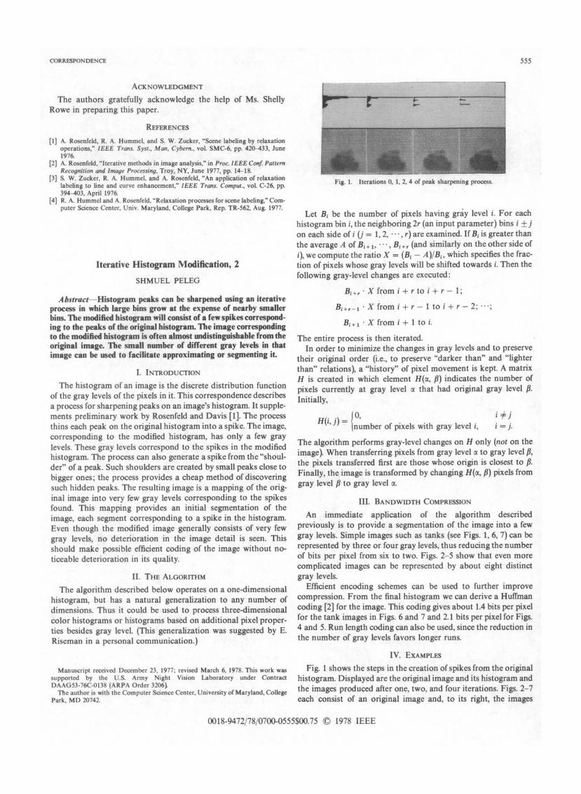
Fig. 1. Iterations 0, 1, 2, 4 of peak sharpening process.

Let Bi be the number of pixels having gray level i. For eachhistogram bin i, the neighboring 2r (an input parameter) bins i + jon each side of i (j = 1, 2, - * *, r) are examined. If B, is greater thanthe average A ofB+ 1, * B+, (and similarly on the other side ofi), we compute the ratio X = (Bi- A)/Bi, which specifies the frac-tion of pixels whose gray levels will be shifted towards i. Then thefollowing gray-level changes are executed:

B -+, X from i + r to i + r - 1;

Bj,,_j Xfrom i +r-1I toi+r -2;--;.

Bj+j *X from i + I to i.

The entire process is then iterated.In order to minimize the changes in gray levels and to preserve

their original order (i.e., to preserve "darker than" and "lighterthan" relations), a "history" of pixel movement is kept. A matrixH is created in which element H(a, P) indicates the number ofpixels currently at gray level a that had original gray level .Initially,

H(i, j) = I0, i *j(number of pixels with gray level i, i =j.

The algorithm performs gray-level changes on H only (not on theimage,\ When transferring pixels from gray level a to gray level P.the pixels transferred first are those whose origin is closest to p.Finally, the image is transformed by changing H(a, P) pixels fromgray level P to gray level a.

III. BANDWIDTH COMPRESSIONAn immediate application of the algorithm described

previously is to provide a segmentation of the image into a fewgray levels. Simple images such as tanks (see Figs. 1, 6, 7) can berepresented by three or four gray levels, thus reducing the numberof bits per pixel from six to two. Figs. 2-5 show that even morecomplicated images can be represented by about eight distinctgray levels.

Efficient encoding schemes can be used to further improvecompression. From the final histogram we can derive a Huffmancoding [2] for the image. This coding gives about 1.4 bits per pixelfor the tank images in Figs. 6 and 7 and 2.1 bits per pixel for Figs.4 and 5. Run length coding can also be used, since the reduction inthe number of gray levels favors longer runs.

IV. EXAMPLESFig. 1 shows the steps in the creation of spikes from the original

histogram. Displayed are the original image and its histogram andthe images produced after one, two, and four iterations. Figs. 2-7each consist of an original image and, to its right, the images

0018-9472/78/0700-0555$00.75 ©) 1978 IEEE

555