Injectivity Conditions of 2D and 3D Uniform Cubic B-Spline Functions

Graphical Models62,411–427 (2000)

doi:10.1006/gmod.2000.0531, available online at http://www.idealibrary.com on

Injectivity Conditions of 2D and 3D UniformCubic B-Spline Functions

Yongchoel Choi and Seungyong Lee1

Department of Computer Science and Engineering, Pohang University of Science and Technology(POSTECH), Pohang, 790-784, Korea

Received December 31, 1999; revised July 15, 2000; accepted August 1, 2000;published online October 13, 2000

Uniform cubic B-spline functions have been used for mapping functions in variousareas such as image warping and morphing, 3D deformation, and volume morphing.The injectivity (one-to-one property) of a mapping function is crucial to obtain-ing desirable results in these areas. This paper considers the injectivity conditionsof 2D and 3D uniform cubic B-spline functions. We propose a geometric interpre-tation of the injectivity of a uniform cubic B-spline function, with which 2D and3D cases can be handled in a similar way. Based on our geometric interpretation,we present sufficient conditions for injectivity which are represented in terms ofcontrol point displacements. These sufficient conditions can be easily tested andwill be useful in guaranteeing the injectivity of mapping functions in applicationareas. c© 2000 Academic Press

1. INTRODUCTION

In computer graphics, mapping functions that transform certain domains into themselvesare widely used. In image warping and morphing, an image is distorted by a 2D mappingfunction that provides a new position for each point in the image [14]. In deformationtechniques such as free-form deformations [12], 3D mapping functions are used to determinethe deformed positions of object points. In volume morphing, user-specified features arealigned by distorting given volumes with 3D mapping functions [2, 10].

In these areas, the injectivity (one-to-one property) of a mapping function is essentialto obtaining good results. In image warping and morphing, if a mapping function is notinjective, the resulting distorted image may contain undesirable wrinkles because partsof the original image are folded upon nearby parts. Several techniques have been devel-oped to generate injective mapping functions for image warping and morphing [3, 7–9].

1 To whom correspondence should be addressed. E-mail: [email protected]. URL:http://www.postech.ac.kr/∼leesy. Fax: +82-54-279-5699.

411

1524-0703/00 $35.00Copyright c© 2000 by Academic Press

All rights of reproduction in any form reserved.

412 CHOI AND LEE

In deformation techniques, the injectivity of a mapping function guarantees that no self-intersection is introduced to an object in the deformation process. In volume morphing,there is no ambiguity in determining the voxel values of a distorted volume provided thatthe mapping function is injective.

Due to their local control property and simplicity, uniform cubic B-spline functions havebeen used for mapping functions in image morphing and 3D deformation. A 2D uniformcubic B-spline function is defined by applying uniform cubic B-spline bases to 2D controlpoints in a 2D control lattice. Similarly, a 3D uniform cubic B-spline function is determinedby a 3D parallelepiped control lattice that consists of 3D control points. Note that each ofthe 2D and 3D B-spline functions is different from a B-spline surface, which is a functionfrom 2D to 3D and is obtained from a 2D control lattice with 3D control points. Leeet al.used2D B-spline functions to efficiently generate mapping functions in image morphing [8, 9].Three-dimensional B-spline functions have been adopted to develop direct manipulationtechniques for free-form deformations [5, 6].

Figure 1 gives an example of the application of 2D B-spline functions to image warping.Figure 1a is the original image with a control lattice overlaid on it. In Fig. 1b, the controllattice is changed to obtain a warped image. Figure 1c shows that a noninjective B-splinefunction generates an undesirable foldover, where the nose is covered with the mouth. InFig. 2, 3D B-spline functions are used to deform a 3D object. Figure 2a shows a sharkwith a control lattice overlaid around the tail. The tail can be deformed by manipulating thecontrol lattice, as shown in Fig. 2b. In Fig. 2c, the 3D B-spline function resulting from thechanged control lattice is not injective and the back part of the tail penetrates the front partin the deformed shape.

To obtain injective mapping functions in image morphing, Leeet al.presented a sufficientcondition for the injectivity of a 2D uniform cubic B-spline function [8, 9]. The sufficientcondition provides a single bound for the displacements of control points that guaranteesthe injectivity of a 2D B-spline function. However, the condition cannot cover the casesin which several control point displacements are above the bound and other are far belowthe bound while the resulting function is still injective. Goodman and Unsworth proposeda sufficient condition for a 2D B´ezier surface to be injective [4], which can be appliedto a 2D B-spline function. For anm× n lattice of control points, the condition contains2m(m+ 1)+ 2n(n+ 1) linear inequalities. Unfortunately, when the number of controlpoints is large, the time to check the condition becomes prohibitive. Although it could beuseful in 3D deformation and volume morphing, there has been no research on an injectivitycondition for a 3D B-spline function.

In this paper, we consider the injectivity conditions of 2D and 3D uniform cubic B-splinefunctions. We first propose a geometric interpretation of the injectivity of a 2D B-splinefunction. Based on this geometric interpretation, we obtain novel sufficient conditionsfor the injectivity of a 2D B-spline function. The sufficient conditions are representedby inequalities of control point displacements and cover more cases than the previousresult [8, 9]. To examine the injectivity condition of a 3D B-spline function, which has notbeen explored yet, we expand the geometric interpretation of injectivity to 3D. Sufficientconditions for the injectivity of a 3D B-spline function are then obtained, which are alsorepresented by inequalities of control point displacements.

The remainder of this paper is organized as follows. In Section 2, we review the mathemat-ical preliminaries. Sections 3 and 4 consider the injectivity conditions of 2D and 3D B-splinefunctions, respectively. Section 5 concludes this paper with future work descriptions.

UNIFORM CUBIC B-SPLINE FUNCTIONS 413

FIG. 1. 2D B-spline functions for image warping.

FIG. 2. 3D B-spline functions for deformation.

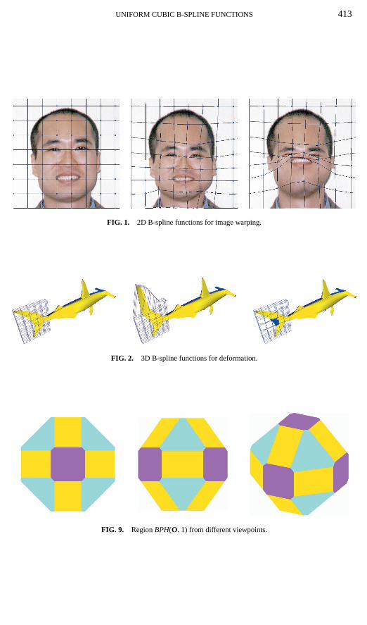
FIG. 9. RegionBPH(O, 1) from different viewpoints.

414 CHOI AND LEE

2. MATHEMATICAL PRELIMINARIES

Let F2 be a 2D uniform cubic B-spline function defined with an (m+ 3)× (n+ 3)control lattice8. FunctionF2 consists ofm× n 2D patches, each of which is determinedby 4× 4 control points inR2. The injectivity of functionF2 may be violated in two cases.First, a global violation of the injectivity happens when a patch ofF2 intersects anotherpatch. Due to the convex hull property of B-splines, this global violation is possible onlyif the control lattice8 contains a self-intersection. Second, the injectivity may be violatedlocally in a patch even though the control lattice8 is not self-intersecting. Although it iscounterintuitive that a B-spline function may not be injective when a control lattice doesnot self-intersect, Leeet al.showed an example of such a configuration [9].

In applications of B-spline functions such as morphing and deformation, the global viola-tion of injectivity is not allowed in most cases and can be prevented by using control latticeswhich are free from self-intersection. Hence, in this paper, we focus on the local injectivityof a B-spline function, which cannot be determined by checking the self-intersection of acontrol lattice.

When we investigate sufficient conditions for the local injectivity of functionF2, it issufficient to consider only one patch ofF2 because the same conditions can be applied toall other patches. Without loss of generality, we represent a 2D uniform cubic B-splinefunction by a patchf2, which is defined by

f2(u, v) = (x, y) =3∑

i=0

3∑j=0

Bi (u)Bj (v)φi j , (1)

where 0≤ u, v ≤ 1. Uniform cubic B-spline basis functions,B0, B1, B2, andB3, are definedby

B0(u) = (1− u)3

6,

B1(u) = 3u3− 6u2+ 4

6,

B2(u) = −3u3+ 3u2+ 3u+ 1

6,

B3(u) = u3

6,

where 0≤ u ≤ 1.φi j = (xi j , yi j ), i, j = 0, 1, 2, 3, are 4× 4 control points that determinefunction f2. Similarly, we represent a 3D uniform cubic B-spline function by a patchf3,which is defined by

f3(u, v, w) = (x, y, z) =3∑

i=0

3∑j=0

3∑k=0

Bi (u)Bj (v)Bk(w)φi jk , (2)

where 0≤ u, v, w ≤ 1.Functions f2 and f3 are locally injective if and only if their Jacobian matrices are non-

singular all over the domain [1]. The Jacobian matrix off2 is defined by

J( f2) =[∂x∂u

∂x∂v

∂y∂u

∂y∂v

].


The Jacobian matrix of functionf3 is defined by

J( f3) =

∂x∂u

∂x∂v

∂x∂w

∂y∂u

∂y∂v

∂y∂w

∂z∂u

∂z∂v

∂z∂w

.It is known that a square matrix is nonsingular if and only if its row vectors are linearlyindependent [13]. Hence, functionf2 is locally injective if and only if two 2D vectors,( ∂x∂u ,

∂x∂v

) and (∂y∂u ,

∂y∂v

), are linearly independent all over the domain. Similarly, functionf3

is locally injective if and only if three 3D vectors, (∂x∂u , ∂x

∂v, ∂x∂w

), ( ∂y∂u , ∂y

∂v, ∂y∂w

), and (∂z∂u ,

∂z∂v

, ∂z∂w

), are linearly independent. In Sections 3 and 4, these conditions are interpretedgeometrically to obtain sufficient conditions for the local injectivity of functionsf2 and f3,respectively.

The following properties of uniform cubic B-spline basis functions and their derivativesare used in later sections.

• Bi (u) ≥ 0, for i = 0, 1, 2, 3• ∑3

i=0 Bi (u) = 1• Bi (u) = B3−i (1− u), for i = 0, 1, 2, 3• ∑3

i=0 |B′i (u)| = −2u2+ 2u+ 1≤ 32

• B′i (u) = −B′3−i (1− u), for i = 0, 1, 2, 3.

3. INJECTIVITY CONDITIONS OF 2D B-SPLINE FUNCTIONS

In this section, we first propose a geometric interpretation of the local injectivity conditionof a 2D uniform cubic B-spline functionf2. The two row vectors in the Jacobian matrixJ( f2)are mapped to two regions inR2 such thatf2 is locally injective if no line simultaneouslypasses through the origin and the two regions. We then obtain sufficient conditions for thelocal injectivity of f2 by computing control point displacements which guarantee such aconfiguration of the two regions.

3.1. Geometric Interpretation of 2D Injectivity

Let f2 be a 2D uniform cubic B-spline function defined by Eq. (1). The injectivityof function f2 is determined by the configuration of the 4× 4 control pointsφi j , i, j =0, 1, 2, 3. Whenφi j equalsφ0

i j = (i − 1, j − 1) for all i, j , function f2 is reduced to anidentity function. Let1φi j be the displacement of control pointφi j fromφ0

i j ; that is1φi j =φi j − φ0

i j = (1xi j ,1yi j ). Then functionf2 can be represented by

f2(u, v) = (u, v)+3∑

i=0

3∑j=0

Bi (u)Bj (v)1φi j .

Now we have

∂x

∂u= 1+

3∑i=0

3∑j=0

Dui j (u, v)1xi j ,

∂x

∂v=

3∑i=0

3∑j=0

Dvi j (u, v)1xi j ,

416 CHOI AND LEE

∂y

∂u=

3∑i=0

3∑j=0

Dui j (u, v)1yi j ,

∂y

∂v= 1+

3∑i=0

3∑j=0

Dvi j (u, v)1yi j ,

whereDui j (u, v) = B′i (u)Bj (v) andDv

i j (u, v) = Bi (u)B′j (v).LetÄ2 be a rectangular domain inR2 that contains points (u, v) such that 0≤ u, v ≤ 1.

Let r1 = ( ∂x∂u , ∂x

∂v) andr2 = ( ∂y

∂u , ∂y∂v

) denote the row vectors of the Jacobian matrixJ( f2).Note thatr1 andr2 are functions fromÄ2 to R2 that depend onu andv. Functionf2 is locallyinjective all over the domainÄ2 if and only if vectorsr1 andr2 are linearly independent foreach (u, v) in Ä2.

A 2D vector (x, y) can be interpreted as a point (x, y) in R2. In this paper, we use a 2Dvector and a point inR2 interchangeably. Two different 2D vectors (x1, y1) and (x2, y2)are linearly independent if and only if the line passing through the two points (x1, y1) and(x2, y2) does not intersect the origin. Hence, functionf2 is locally injective overÄ2 if andonly if no line simultaneously passes through the origin,r1, andr2 for any (u, v) in Ä2.

Let S2(c, δ) be a region inR2 defined by

S2(c, δ) =(x + cx, y+ cy) | x =

3∑i=0

3∑j=0

Dui j (u, v)δi j , y =

3∑i=0

3∑j=0

Dvi j (u, v) δi j

,where c= (cx, cy), |δi j | ≤ δ, and 0≤ u, v ≤ 1. Let e1 = (1, 0) and e2 = (0, 1). Then,S2(e1, δx) is the set of all possible values ofr1 from the configurations of control pointsφi j

that satisfy|1xi j | ≤ δx. Similarly, S2(e2, δy) contains all possible values ofr2 under theconstraint|1yi j | ≤ δy. Figure 3 shows a schematic diagram ofS2(e1, δx) andS2(e2, δy).

Let δx = max{|1xi j |} andδy = max{|1yi j |}. Then, for any (u, v) in Ä2, r1 andr2 arecontained inS2(e1, δx) and S2(e2, δy), respectively. Suppose that no line simultaneouslyintersects the origin,S2(e1, δx), andS2(e2, δy) as shown in Fig. 3. In this case, for each (u, v)in Ä2, no line can simultaneously passes through the origin,r1, andr2 and hence function

FIG. 3. A schematic diagram ofS2(e1, δx) andS2(e2, δy).


f2 is locally injective. The following lemma summarizes the relationship ofS2(e1, δx) andS2(e2, δy) with the local injectivity of functionf2.

LEMMA 1. Function f2 is locally injective all over the domain if no line simultaneouslypasses through the origin, S2(e1, δx), and S2(e2, δy).

To determine the values ofδx andδy that satisfy the condition in Lemma 1, it is necessaryto represent the shape ofS2(c, δ) in terms ofc andδ. Since it is not easy to analyze theexact shape ofS2(c, δ), we find two simple regions inR2 that includeS2(c, δ). The shapeof S2(c, δ) can then be approximated by the intersection of the two regions.

3.2. Bounding Regions of S2(c, δ)

Let BS(c, δ) be a rectangular region inR2 defined by

BS(c, δ) ={

(x + cx, y+ cy) | |x| ≤ 3

2δ, |y| ≤ 3

2δ

},

wherec= (cx, cy). Let O denote the origin inR2. Figure 4a shows the configuration ofBS(O, δ). It is simple to verify thatBS(c, δ) is a bounding region ofS2(c, δ) by using theproperties of uniform cubic B-spline basis functions. In the proofs of the following lemmasabout bounding regions, without loss of generality, we only consider the case whenc is theorigin O.

LEMMA 2. S2(c, δ) ⊂ BS(c, δ).

Proof. For each point (x, y) ∈ S2(O, δ), we have

|x| =∣∣∣∣∣

3∑i=0

3∑j=0

Dui j (u, v)δi j

∣∣∣∣∣≤

3∑i=0

|B′i (u)|3∑

j=0

Bj (v)δ

≤ 3

2δ.

Similarly, we can show that|y| ≤ 32δ.

FIG. 4. Regions (a)BS(O, δ) and (b)BD(O, δ).

418 CHOI AND LEE

To obtain the second bounding region ofS2(c, δ), we introduce a constantK2 that isrelated to uniform cubic B-spline basis functions,

K2 = max0≤u,v≤1

{g2(u, v)},

where

g2(u, v) =3∑

i=0

3∑j=0

∣∣Dui j (u, v)+ Dv

i j (u, v)∣∣.

To compute the value ofK2, the domainÄ2 = {(u, v) | 0≤ u, v ≤ 1} is partitioned to a verydense grid with the grid spacing 10−10. We then evaluate the functiong2 at every grid point,and the maximum occurs at (u0, u0), whereu0 = 0.2448210078 oru0 = 0.7551789922.Thus,K2 is approximately 2.046392675.

Let BD(c, δ) be a region inR2 defined by

BD(c, δ) = {(x + cx, y+ cy) | |x + y| ≤ K2δ, |x − y| ≤ K2δ}.

Figure 4b shows the configuration ofBD(O, δ). The following lemma shows thatBD(c, δ)is a bounding region ofS2(c, δ).

LEMMA 3. S2(c, δ) ⊂ BD(c, δ).

Proof. Let Rz(S2(O, δ)) be the region inR2 that corresponds to the rotation ofS2(O, δ)by−π

4 with respect to the origin,

Rz(S2(O, δ)) ={

(x′, y′) | x′ = 1√2

(x + y), y′ = 1√2

(−x + y)

},

where (x, y) ∈ S2(O, δ). Let Rz(BD(O, δ)) be the rotation ofBD(O, δ) by−π4 with respect

to the origin,

Rz(BD(O, δ)) ={

(x′, y′) | |x′| ≤ K2√2δ, |y′| ≤ K2√

2δ

}.

For each point (x′, y′) ∈ Rz(S2(O, δ)), we have

|x′| =∣∣∣∣∣ 1√

2

3∑i=0

3∑j=0

(Du

i j (u, v)+ Dvi j (u, v)

)δi j

∣∣∣∣∣≤ 1√

2

3∑i=0

3∑j=0

∣∣Dui j (u, v)+ Dv

i j (u, v)∣∣|δi j |

≤ K2√2δ.

Similarly, we can show that|y′| ≤ K2√2δ by using

K2 = max0≤u,v≤1

{3∑

i=0

3∑j=0

∣∣Dui j (u, v)− Dv

i j (u, v)∣∣},


FIG. 5. Regions (a)BP(O, δ) and (b)BC(O, δ).

which holds from Bj (v) = B3− j (1− v) and B′j (v) = −B′3− j (1− v). Then we haveRz(S2(O, δ)) ⊂ Rz(BD(O, δ)), which impliesS2(O, δ) ⊂ BD(O, δ).

Let BP(c, δ) be the intersection ofBS(c, δ) andBD(c, δ):

BP(c, δ) = BS(c, δ) ∩ BD(c, δ).

Figure 5a shows the configuration ofBP(O, δ). It trivially holds thatBP(c, δ) is a polygonalbounding region ofS2(c, δ).

LEMMA 4. S2(c, δ) ⊂ BP(c, δ).

Let BC(c, δ) be a circular region inR2 defined by

BC(c, δ) = {(x + cx, y+ cy) | x2+ y2 ≤ (A2δ)2},

wherec= (cx, cy) and

A2 =√(

3

2

)2

+(

K2− 3

2

)2

.

BC(c, δ) is the smallest circular region that enclosesBP(c, δ). Figure 5b shows the config-uration ofBC(O, δ) overlaid onBP(O, δ). It is obvious thatBC(c, δ) is a circular boundingregion ofS2(c, δ).

LEMMA 5. S2(c, δ) ⊂ BC(c, δ).

3.3. Sufficient Conditions for 2D Injectivity

With the geometric interpretation presented in Section 3.1 and the bounding regionsobtained in Section 3.2, we can derive sufficient conditions for the local injectivity ofa 2D uniform cubic B-spline function. Letf2 be the function defined by Eq. (1) and1φi j = φi j − φ0

i j = (1xi j ,1yi j ) for i, j = 0, 1, 2, 3. Let δx = max{|1xi j |} and δy =max{|1yi j |}.

420 CHOI AND LEE

FIG. 6. The configuration ofBP(e1,1

K2) andBP(e2,

1K2

).

THEOREM1. Function f2 is locally injective all over the domain ifδx <1

K2andδy <

1K2

.

Proof. Suppose thatδx <1

K2and δy <

1K2

. Then we haveBP(e1, δx) ⊂ {(x, y) | x +y > 0, x − y > 0} andBP(e2, δy) ⊂ {(x, y) | x + y > 0, x − y < 0} (see Fig. 6). Hence,no line that passes through the origin can intersect bothBP(e1, δx) andBP(e2, δy). FromLemma 4, this implies that no line simultaneously passes through the origin,S2(e1, δx), andS2(e2, δy). Then, from Lemma 1, functionf2 is locally injective all over the domain.

In Theorem 1, the sufficient condition for local injectivity provides the same bound forthe x- andy-displacements of control points. This condition cannot cover cases in whichfunction f2 may be locally injective ifδy is much smaller than1

K2thoughδx ≥ 1

K2. We can

obtain a sufficient condition that can handle such a case by using the circular boundingregionBC(c, δ). We first show a lemma related to a line passing through the origin andregionsBC(e1, δx) andBC(e2, δy).

LEMMA 6. If there is a line that simultaneously passes through the origin, BC(e1, δx),and BC(e2, δy), thenδ2

x + δ2y ≥ ( 1

A2)2.

Proof. Let l be a line that passes through the origin, which is represented byax+ by=0. Let d1 and d2 be the distances ofe1 and e2 from line l , respectively. Then we haved1 = |a|/

√a2+ b2 andd2 = |b|/

√a2+ b2, which givesd2

1 + d22 = 1. Suppose that linel

simultaneously intersectsBC(e1, δx) andBC(e2, δy). Figure 7 shows an example of such a

FIG. 7. A configuration ofBC(e1, δx) andBC(e2, δy) with a line passing through the origin.


configuration. Then we haved1 ≤ A2δx andd2 ≤ A2δy. This implies that 1= d21 + d2

2 ≤A2

2(δ2x + δ2

y).

THEOREM2. Function f2 is locally injective all over the domain ifδ2x + δ2

y < ( 1A2

)2.

Proof. Suppose thatδ2x + δ2

y < ( 1A2

)2. Then, from Lemma 6, there cannot be a linepassing through the origin that simultaneously intersectsBC(e1, δx) andBC(e2, δy). Thisimplies from Lemmas 1 and 5 that functionf2 is locally injective all over the domain.

Since the constantK2 is approximately 2.046392675, the bounds1K2

and ( 1A2

)2 given inTheorems 1 and 2 are approximately 0.488664767 and 0.392380757, respectively. Thus itseems that the sufficient conditions in Theorems 1 and 2 only provide very small bounds forcontrol point displacements. However, by using the affine invariance property of B-splines,we can extend Theorems 1 and 2 to handle general cases with possibly large control pointdisplacements. That is, we can apply the bounds to the normalized values of control pointdisplacements instead of the given values.

To normalize the control point displacements, we consider a 2D affine transformationM2 that moves the given control pointsφi j toward the canonical positionsφ0

i j . Letφ′i j be thenew position of a control pointφi j when it is transformed byM2. We determine the affinetransformationM2 so that it minimizes the approximation error,

∑3i=0

∑3j=0 ‖φ′i j − φ0

i j ‖2.Such a transformationM2 can simply be obtained by using the matrix representation ofM2. For details of inferring an affine transformation from a set of corresponding pointpairs and the least-squares solution of a linear system, refer to the references [11, 14]. Let1φ′i j = φ′i j − φ0

i j = (1x′i j ,1y′i j ). Let δ′x = max{|1x′i j |} andδ′y = max{|1y′i j |}.THEOREM3. Function f2 is locally injective all over the domain if the 2D affine trans-

formation M2 is invertible and ifδ′x andδ′y satisfy one of the conditionsδ′x <1

K2andδ′y <

1K2

or (δ′x)2+ (δ′y)2 < ( 1A2

)2.

Proof. Let f ′2 be the 2D uniform cubic B-spline function determined by transformedcontrol pointsφ′i j . If δ′x <

1K2

andδ′y <1

K2or if (δ′x)2+ (δ′y)2 < ( 1

A2)2, function f ′2 is locally

injective all over the domain from Theorem 1 or Theorem 2, respectively. Due to the affineinvariance property of B-splines, the function valuef2(u, v) is mapped to the functionvalue f ′2(u, v) by transformationM2. If M2 is invertible, the mapping betweenf2(u, v) andf ′2(u, v) is a one-to-one correspondence.

For example, when control point displacements1φi j are (5, 5) for alli, j , it is obviousthat function f2 is locally injective all over the domain. However, Theorems 1 and 2 do notcover this case because the conditions in them are not satisfied by1φi j = (5, 5). In contrast,when we normalize the displacements1φi j , transformationM2 is a translation by (−5,−5)and1φ′i j = (0, 0) for all i, j , which obviously satisfies the condition in Theorem 3.

The sufficient conditions in Theorems 1 and 2 are not necessary for the local injectivityof function f2 even if we apply them to the normalized control point displacements. Forexample, let1x0 j = 1x1 j = −1x2 j = −1x3 j = 0.65 and1yi j = 0, for i, j = 0, 1, 2, 3.In this case, both of the conditions in Theorems 1 and 2 are violated but functionf2 is stilllocally injective.

However, the bound for the control point displacements in Theorem 1 is tight. Leeet al. [9] presented a control lattice configuration with which functionf2 is not locallyinjective whenδx = δy = 1

K2. In the configuration,1xi j = 1yi j = 1

K2if i + j ≤ 3 and

1xi j = 1yi j = − 1K2

if i + j > 3 for i, j = 0, 1, 2, 3. Then the Jacobian|J( f2)| vanishes

422 CHOI AND LEE

for the point (u0, u0) at which the functiong2 has the maximum valueK2. For Theorem 2,we have not yet fully investigated the tightness of the inequality in it.

Theorem 2 is more useful than Theorem 1 whenδx andδy are different. For example,given a control lattice withδx = 0.62 andδy = 0, we cannot verify the local injectivity ofthe resulting functionf2 with Theorem 1. In contrast, Theorem 2 can be used to guaranteethat the functionf2 is locally injective.

4. INJECTIVITY CONDITIONS OF 3D B-SPLINE FUNCTIONS

In this section, we present sufficient conditions for the local injectivity of a 3D uniformcubic B-spline function by expanding the geometric interpretation and the bounding regionspresented in Section 3 to 3D space.

4.1. Geometric Interpretation of 3D Injectivity

Let f3 be a 3D uniform cubic B-spline function defined by Eq. (2). Whenφi jk equalsφ0

i jk = (i − 1, j − 1, k− 1) for i, j, k = 0, 1, 2, 3, functionf3 is reduced to an identityfunction. Let1φi jk be the displacement of control pointφi jk from φ0

i jk ; that is,1φi jk =φi jk − φ0

i jk = (1xi jk ,1yi jk ,1zi jk ). Then we have

f3(u, v, w) = (u, v, w)+3∑

i=0

3∑j=0

3∑k=0

Bi (u)Bj (v)Bk(w)1φi jk .

Let r1 = ( ∂x∂u ,

∂x∂v, ∂x∂w

), r2 = ( ∂y∂u ,

∂y∂v,∂y∂w

), and r3 = ( ∂z∂u ,

∂z∂v, ∂z∂w

) denote the row vec-tors of the Jacobian matrixJ( f3). Let Du

i jk (u, v, w)= B′i (u)Bj (v)Bk(w), Dvi jk (u, v, w)=

Bi (u)B′j (v)Bk(w), andDwi jk (u, v, w) = Bi (u)Bj (v)B′k(w). We defineS3(c, δ) as a region in

R3 such that

S3(c, δ) ={

(x + cx, y+ cy, z+ cz) | x =3∑

i=0

3∑j=0

3∑k=0

Dui jk (u, v, w)δi jk ,

y =3∑

i=0

3∑j=0

3∑k=0

Dvi jk (u, v, w)δi jk , z=

3∑i=0

3∑j=0

3∑k=0

Dwi jk (u, v, w)δi jk

},

wherec= (cx, cy, cz), |δi jk | ≤ δ, and 0≤ u, v, w ≤ 1. S3(c, δ) is the 3D expansion ofthe regionS2(c, δ). Let e1 = (1, 0, 0), e2 = (0, 1, 0), ande3 = (0, 0, 1). Figure 8 shows aschematic diagram of the regionsS3(e1, δx), S3(e2, δy), andS3(e3, δz).

Let δx = max{|1xi jk |}, δy = max{|1yi jk |}, andδz = max{|1zi jk |}. The 3D extension ofLemma 1 can easily be proved from the fact that three vectorsr1, r2, and r3 in R3 arelinearly independent if and only if there is no plane passing through the origin that containsthe pointsr1, r2, andr3. As in the 2D case, we interchangeably use a 3D vector and a pointin R3.

LEMMA 7. Function f3 is locally injective all over the domain if no plane simultaneouslypasses through the origin, S3(e1, δx), S3(e2, δy), and S3(e3, δz).


FIG. 8. A schematic diagram ofS3(e1, δx), S3(e2, δy), andS3(e3, δz).

4.2. Bounding Regions of S3(c, δ)

Let BTS(c, δ) be a region inR3 defined by

BTS(c, δ) ={

(x + cx, y+ cy, z+ cz) | |x| ≤ 3

2δ, |y| ≤ 3

2δ, |z| ≤ 3

2δ

},

wherec= (cx, cy, cz). It can be proved in a similar way to Lemma 2 thatBTS(c, δ) is abounding region ofS3(c, δ).

LEMMA 8. S3(c, δ) ⊂ BTS(c, δ).

Let BTD(c, δ) be a region inR3 defined by

BTD(c, δ) = BTX(c, δ) ∩ BTY(c, δ) ∩ BTZ(c, δ),

where

BTX(c, δ) ={

(x + cx, y+ cy, z+ cz) | |x| ≤ 3

2δ, |y+ z| ≤ K2δ, |y− z| ≤ K2δ

},

BTY(c, δ) ={

(x + cx, y+ cy, z+ cz) | |y| ≤ 3

2δ, |z+ x| ≤ K2δ, |z− x| ≤ K2δ

},

BTZ(c, δ) ={

(x + cx, y+ cy, z+ cz) | |z| ≤ 3

2δ, |x + y| ≤ K2δ, |x − y| ≤ K2δ

},

andc= (cx, cy, cz). Note thatBTZ(c, δ) is an extrusion of the 2D regionBD(c, δ) in thez-direction. Similarly,BTX(c, δ) andBTY(c, δ) are extrusions ofBD(c, δ) when it is definedin the yz- andzx-planes, respectively. It is simple to show thatBTD(c, δ) is a boundingregion ofS3(c, δ).

LEMMA 9. S3(c, δ) ⊂ BTD(c, δ).

424 CHOI AND LEE

Proof. It can be shown thatS3(O, δ) ⊂ BTZ(O, δ) in a way similar to Lemma 3. Also,we can show thatS3(O, δ) ⊂ BTX(O, δ) andS3(O, δ) ⊂ BTY(O, δ) by using rotations withrespect to thex- andy-axes, respectively.

To obtain a regular octahedron that includesS3(c, δ), we introduce a constantK3, whichis the 3D correspondence ofK2,

K3 = max0≤u,v,w≤1

{g3(u, v, w)},

where

g3(u, v, w) =3∑

i=0

3∑j=0

3∑k=0

∣∣Dui jk (u, v, w)+ Dv

i jk (u, v, w)+ Dwi jk (u, v, w)

∣∣.To compute the value ofK3, the domain,Ä3 = {(u, v, w) | 0≤ u, v, w ≤ 1}, is partitionedinto a very dense grid with the grid spacing 10−10. We then evaluate the functiong3 atevery grid point, and the maximum occurs at (u0, u0, u0), whereu0 = 0.1640662347 oru0 = 0.8359337653. Thus,K3 is approximately 2.479472335.

Let BTO(c, δ) be a region inR3 defined by

BTO(c, δ) = BTP1(c, δ) ∩ BTP2(c, δ) ∩ BTP3(c, δ) ∩ BTP4(c, δ),

where

BTP1(c, δ) = {(x + cx, y+ cy, z+ cz) | |x + y+ z| ≤ K3δ},BTP2(c, δ) = {(x + cx, y+ cy, z+ cz) | |x + y− z| ≤ K3δ},BTP3(c, δ) = {(x + cx, y+ cy, z+ cz) | |x − y+ z| ≤ K3δ},BTP4(c, δ) = {(x + cx, y+ cy, z+ cz) | |x − y− z| ≤ K3δ}

andc= (cx, cy, cz). The following lemma shows thatBTO(c, δ) is a bounding region ofS3(c, δ).

LEMMA 10. S3(c, δ) ⊂ BTO(c, δ).

Proof. Consider a 3D rotationRxy that maps the vector (1, 1, 1) onto thez-axis. RotationRxy transformsBTP1(O, δ) to Rxy(BTP1(O, δ)), where

Rxy(BTP1(O, δ)) ={

(x′, y′, z′) | |z′| ≤ K3√3δ

}.

Let z′ be thez-coordinate of the new position when we apply rotationRxy to a point(x, y, z) ∈ S3(O, δ). Then we have

|z′| =∣∣∣∣ 1√

3(x + y+ z)

∣∣∣∣≤ 1√

3

3∑i=0

3∑j=0

3∑k=0

∣∣Dui jk (u, v, w)+ Dv

i jk (u, v, w)+ Dwi jk (u, v, w)

∣∣|δi jk |

≤ K3√3δ,


which impliesS3(O, δ) ⊂ BTP1(O, δ). Similarly, we can show thatS3(O, δ) ⊂ BTP2(O, δ)S3(O, δ) ⊂ BTP3(O, δ), andS3(O, δ) ⊂ BTP4(O, δ).

Let BPH(c, δ) be the intersection ofBTS(c, δ),BTD(c, δ), andBTO(c, δ):

BPH(c, δ) = BTS(c, δ) ∩ BTD(c, δ) ∩ BTO(c, δ).

The boundary ofBPH(c, δ) consists of 26 faces. Figure 9 illustrates the shape ofBPH(O, 1).Figure 9a is the shape ofBPH(O, 1) that is seen from thex-axis toward the origin. Notethat, due to the symmetry, the shape is the same whenBPH(O, 1) is seen from they- orz-axis. The shape in Fig. 9b is obtained when we look atBPH(O, 1) from the liney = x inthexy-plane toward the origin. Figure 9c shows the shape ofBPH(O, 1) with a viewpointlooking downward. In Fig. 9, magenta, yellow, and cyan faces are originally part of the facesof BTS(O, 1), BTD(O, 1), andBTO(O, 1), respectively. It trivially holds thatBPH(c, δ) is apolyhedral bounding region ofS3(c, δ).

LEMMA 11. S3(c, δ) ⊂ BPH(c, δ).

Let BSP(c, δ) be a spherical region defined by

BSP(c, δ) = {(x + cx, y+ cy, z+ cz) | x2+ y2+ z2 ≤ (A3δ)2},

wherec= (cx, cy, cz) and

A3 =√(

3

2

)2

+(

K2− 3

2

)2

+ (K3− K2)2.

BSP(c, δ) is the smallest spherical region that enclosesBPH(c, δ). It is obvious thatBSP(c, δ)is a bounding region ofS3(c, δ).

LEMMA 12. S3(c, δ) ⊂ BSP(c, δ).

4.3. Sufficient Conditions for 3D Injectivity

Now we present sufficient conditions for the local injectivity of a 3D uniform cubic B-spline function. Letf3 be the function defined by Eq. (2) and let1φi jk = φi jk − φ0

i jk =(1xi jk ,1yi jk ,1zi jk ) for i, j, k = 0, 1, 2, 3. Letδx = max{|1xi jk |}, δy = max{|1yi jk |}, andδz = max{|1zi jk |}.

THEOREM 4. Function f3 is locally injective all over the domain ifδx <1

K3, δy <

1K3,

andδz <1

K3.

Proof. By using the polyhedral bounding regionBPH(c, δ) of S3(c, δ), this theorem canbe proved in a way similar to Theorem 1.

THEOREM5. Function f3 is locally injective all over the domain ifδ2x + δ2

y + δ2z< ( 1

A3)2.

Proof. Using the spherical bounding regionBSP(c, δ) of S3(c, δ), this theorem can beproved in a way similar to Theorem 2.

To normalize the control point displacements, we consider a 3D affine transforma-tion M3. Let φ′i jk be the new position of a control pointφi jk when it is transformed by

426 CHOI AND LEE

M3. We determine the affine transformationM3 so that it minimizes the approximationerror,

∑3i=0

∑3j=0

∑3k=0 ‖φ′i jk − φ0

i jk‖2. Let 1φ′i jk = φ′i jk − φ0i jk = (1x′i jk ,1y′i jk ,1z′i jk ).

Let δ′x = max{|1x′i jk |}, δ′y = max{|1y′i jk |}, andδ′z = max{|1z′i jk |}.THEOREM6. Function f3 is locally injective all over the domain if the 3D affine transfor-

mation M3 is invertible and ifδ′x, δ′y, andδ′z satisfy one of the conditionsδ′x <

1K3, δ′y <

1K3,

andδ′z <1

K3or (δ′x)2+ (δ′y)2+ (δ′z)

2 < ( 1A3

)2.

Proof. By using the affine invariance property of B-splines, this theorem can be provedin a way similar to Theorem 3.

As in the 2D case, the sufficient conditions in Theorems 4 and 5 are not necessary forthe local injectivity of functionf3. However, similarly to Theorem 1, Theorem 4 provides atight bound for the control point displacements. There is a control lattice configuration withwhich f3 is not locally injective whenδx = δy = δz = 1

K3. In the configuration,1xi jk =

1yi jk = 1zi jk = 1K3

if i + j + k ≤ 3 and1xi j = 1yi j = 1zi jk = − 1K2

if i + j + k > 3for i, j, k = 0, 1, 2, 3. Then the Jacobian|J( f3)| vanishes for the point (u0, u0, u0) at whichthe functiong3 has the maximum valueK3. We have not yet fully investigated the tightnessof the inequality in Theorem 5.

5. CONCLUSIONS

In this paper, we have presented sufficient conditions for the local injectivity of 2D and3D uniform cubic B-spline functions. We first proposed a geometric interpretation of thelocal injectivity of a uniform cubic B-spline function. Row vectors in the Jacobian matrix aremapped to regions in the space, for which we obtained simple bounding regions. Sufficientconditions represented in terms of control point displacements were finally derived by usingthe bounding regions. These sufficient conditions are straightforward and easily tested sothat they may be useful to guarantee the injectivity of mapping functions in applicationssuch as image warping and morphing, 3D deformation, and volume morphing.

Future work will involve an investigation of sufficient conditions that consider eachcontrol point displacement independently. In this paper, sufficient conditions are representedonly in terms of the maximums of the control point displacements in principal directions.The ultimate future goal will be to obtain simple and easy-to-check necessary and sufficientconditions for the injectivity of uniform cubic B-spline functions.

ACKNOWLEDGMENTS

This work was supported by the University Research Program of the Ministry of Information and Communica-tion in South Korea (Grant 2NI9890701). Additional support was provided by the Ministry of Education of Koreathrough the Brain Korea 21 program.

REFERENCES

1. R. C. Buck,Advanced Calculus, 3rd ed., McGraw–Hill, New York, 1978.

2. D. Cohen-Or, A. Solomovic, and D. Levin, Three-dimensional distance field metamorphosis,ACM Trans.Graphics17(2), 1998, 116–141.

3. K. Fujimura and M. Makarov, Foldover-free image warping,Graphical Models Image Process.60, 1998,100–111.


4. T. Goodman and K. Unsworth,Injective Bivariate Maps, Technical Report CS94/02, Dundee University, 1994.

5. M. Hagenlocker and K. Fujimura, CFFD: A tool for designing flexible shapes,Visual Comput.14(5), 1998,271–287.

6. W. M. Hsu, J. F. Hughes, and H. Kaufman, Direct manipulation of free-form deformations, inProceedings ofSIGGRAPH ’92, ACM Comput. Graphics26(2), 1992, 177–184.

7. S. Lee, K.-Y. Chwa, J. Hahn, and S. Y. Shin, Image morphing using deformation techniques,J. Visualizat.Comput. Animat.7(1), 1996, 3–23.

8. S. Lee, K.-Y. Chwa, S. Y. Shin, and G. Wolberg, Image metamorphosis using snakes and free-form deforma-tions, inProceedings of SIGGRAPH ’95, ACM Comput. Graphics, 1995, 439–448.

9. S. Lee, G. Wolberg, K.-Y. Chwa, and S. Y. Shin, Image metamorphosis with scattered feature constraints,IEEE Trans. Visualizat. Comput. Graphics2(4), 1996, 337–354.

10. A. Lerios, C. D. Garfinkle, and M. Levoy, Feature-based volume metamorphosis, inProceedings ofSIGGRAPH ’95, ACM Comput. Graphics, 1995, 449–456.

11. W. H. Press, S. A. Teukolsky, W. T. Vetterling, and B. P. Flannery,Numerical Recipes in C, 2nd ed., CambridgeUniv. Press, Cambridge, UK, 1992.

12. T. W. Sederberg and S. R. Parry, Free-form deformation of solid geometric models,ACM Comput. Graphics(Proc. of SIGGRAPH ’86)20(4), 1986, 151–160.

13. G. Strang,Linear Algebra and Its Applications, 3rd ed., Harcourt Brace Jovanovich, San Diego, 1988.

14. G. Wolberg,Digital Image Warping, IEEE Comput. Soc. Press, Los Alamitos, CA, 1990.

Injectivity Conditions of 2D and 3D Uniform Cubic B-Spline Functions

Documents

Transcript of Injectivity Conditions of 2D and 3D Uniform Cubic B-Spline Functions