Implementation and performance evaluation of different cubic ...
35
http://lib.ulg.ac.be http://matheo.ulg.ac.be Implementation and performance evaluation of different cubic equations of state for the estimation of properties of organic mixtures Auteur : Welliquet, Jonathan Promoteur(s) : Quoilin, Sylvain Faculté : Faculté des Sciences appliquées Diplôme : Master en ingénieur civil électromécanicien, à finalité approfondie Année académique : 2015-2016 URI/URL : https://github.com/CoolProp/CoolProp; http://hdl.handle.net/2268.2/2013 Avertissement à l'attention des usagers : Tous les documents placés en accès ouvert sur le site le site MatheO sont protégés par le droit d'auteur. Conformément aux principes énoncés par la "Budapest Open Access Initiative"(BOAI, 2002), l'utilisateur du site peut lire, télécharger, copier, transmettre, imprimer, chercher ou faire un lien vers le texte intégral de ces documents, les disséquer pour les indexer, s'en servir de données pour un logiciel, ou s'en servir à toute autre fin légale (ou prévue par la réglementation relative au droit d'auteur). Toute utilisation du document à des fins commerciales est strictement interdite. Par ailleurs, l'utilisateur s'engage à respecter les droits moraux de l'auteur, principalement le droit à l'intégrité de l'oeuvre et le droit de paternité et ce dans toute utilisation que l'utilisateur entreprend. Ainsi, à titre d'exemple, lorsqu'il reproduira un document par extrait ou dans son intégralité, l'utilisateur citera de manière complète les sources telles que mentionnées ci-dessus. Toute utilisation non explicitement autorisée ci-avant (telle que par exemple, la modification du document ou son résumé) nécessite l'autorisation préalable et expresse des auteurs ou de leurs ayants droit.
-
Upload
khangminh22 -
Category
Documents
-
view
0 -
download
0
Transcript of Implementation and performance evaluation of different cubic ...
httplibulgacbe httpmatheoulgacbe
Implementation and performance evaluation of different cubic equations of
state for the estimation of properties of organic mixtures
Auteur Welliquet Jonathan
Promoteur(s) Quoilin Sylvain
Faculteacute Faculteacute des Sciences appliqueacutees
Diplocircme Master en ingeacutenieur civil eacutelectromeacutecanicien agrave finaliteacute approfondie
Anneacutee acadeacutemique 2015-2016
URIURL httpsgithubcomCoolPropCoolProp httphdlhandlenet226822013
Avertissement agrave lattention des usagers
Tous les documents placeacutes en accegraves ouvert sur le site le site MatheO sont proteacutegeacutes par le droit dauteur Conformeacutement
aux principes eacutenonceacutes par la Budapest Open Access Initiative(BOAI 2002) lutilisateur du site peut lire teacuteleacutecharger
copier transmettre imprimer chercher ou faire un lien vers le texte inteacutegral de ces documents les disseacutequer pour les
indexer sen servir de donneacutees pour un logiciel ou sen servir agrave toute autre fin leacutegale (ou preacutevue par la reacuteglementation
relative au droit dauteur) Toute utilisation du document agrave des fins commerciales est strictement interdite
Par ailleurs lutilisateur sengage agrave respecter les droits moraux de lauteur principalement le droit agrave linteacutegriteacute de loeuvre
et le droit de paterniteacute et ce dans toute utilisation que lutilisateur entreprend Ainsi agrave titre dexemple lorsquil reproduira
un document par extrait ou dans son inteacutegraliteacute lutilisateur citera de maniegravere complegravete les sources telles que
mentionneacutees ci-dessus Toute utilisation non explicitement autoriseacutee ci-avant (telle que par exemple la modification du
document ou son reacutesumeacute) neacutecessite lautorisation preacutealable et expresse des auteurs ou de leurs ayants droit
Implementation and performance evaluation of different cubic equations ofstate for the estimation of properties of organic mixtures
Jonathan WelliquetUniversity of Liegravege Faculty of Applied Sciences
Aerospace and mechanical engineering departmentThermodynamic Laboratory
Abstract
The thermodynamic properties of organic mixtures is a really important aspect for the development ofthe new thermodynamic cycles However mixtures are not all yet well known and a model that could givea good approximation of the properties in a fast way could help
The cubic equations of states provide a simple way requiring minimal information to approximate thestate of a fluid This provide an interesting tool with enough flexibility to improve the accuracy as moreexperimental data become available The results for vapour-liquid equilibrium of mixtures are particularlygood
Keywords CoolProp Cubic EOS Mixtures
URL httpwwwfacsaulgacbe (Jonathan Welliquet)
Preprint submitted to Thermodynamic Laboratory August 20 2016
Contents
1 Introduction 3
2 State of the art 421 Cubic Equations of State 4
211 Soave-Redlich-Kwong 4212 Peng-Robinson 4213 Volume translation 5214 VTPR 6
22 Mixing rules 823 Software 8
231 RefProp 8232 CoolProp 8
3 Volume translation implementation 931 Solving the cubic equation 932 Preparing for the other thermodynamic properties 9
4 Comparison 1141 Pure fluid 1142 Binary mixtures 2243 Ternary mixtures 29
5 Acknowledgements 32
6 Conclusions 33
2
1 Introduction
The improvements in thermodynamic cycles relies on the possibility to chose the most suitable fluid andto model it accurately
Thermodynamic libraries likes RefProp FluidProp and CoolProp provides efficient models for sufficientlywell known fluids (mainly through Helmholtz equation of state or interpolation from experimental data)However there are still a lack of data for less studied fluids particularly mixtures which usually need exper-imental data to evaluate the interaction parameters required for the models These interaction parameterare often approximated or not used at all
Accurate models like the Helmholtz equations of state (HEOS) usually require a consequent numberof experimental data whereas the cubic equations of state are simpler model that can already gives goodresults with very few experimental data (critical pressure and temperature pcrit Tcrit and acentric factor ω)Being simpler models they also have the benefit from being faster Of course these advantages comes at thecost of a lower accuracy These cubic models can be enhanced by some parameters (approximated or fittedto experimental data) to increase their accuracy
The cubic equations of state are thus a good candidate to have a fast model to approximate the behaviourof non yet well studied fluids This is extremely helpful in the research field where this allows to quicklyevaluate a lot of potentials fluids and select the one worthy of interest before running expensive experimentalsetup to evaluate more accurately their behaviour
The scope of this work is to evaluate what can be expected from these Cubic equations of state A focuswill be set on organic mixtures relevant for refrigeration and heat pump applications The implementationa simple volume translation model has also been proceed and is explained in this report
3
2 State of the art
21 Cubic Equations of StateThe thermodynamic state of a fluid can be defined by two independent state variables An equations
of state (EOS) is a relation between state variables generally aiming to compute a third variable from twoother known ones
Cubic equations of state have of cubic that they can be expressed as a cubic equation of the molarvolume v
The first cubic equation of state was the so called Van der Waals equation of state and of the form(p +
av2
)(v minus b) = RT (1)
With the a and b parameters depending on the critical pressure and critical molar volumeThis equation 1 is linking the pressure p the molar volume v and the temperature T Theses kind of
equations are generally referred as PVTEOS and have the advantage to provide both the liquid and vapourphases with a single equation (Frey et al 2007)
With time some improvements have been added to improve the quality of the approximation in boththe general formula and in the way to compute the attraction parameter a and the repulsion parameter (oreffective molecular volume) bThe attractive parameter is often separated in a constant part ac multiplied by a temperature dependantone α(TR ω) such as a = acα(TR ω)
The most common equations of state used in process simulation are mainly based on the Soave-Redlich-Kwong and Peng-Robinson EOS (Frey et al 2007)
211 Soave-Redlich-KwongThe Soave-Redlich-Kwong (SRK) is an improved Redlich-Kwong equation of state and has the original
form (Soave 1972)
p =RT
v minus bminus
acα(TR ω)
v(v + b)(2)
With the parameters
ac = 042747
(R2T2
c
Pc
)b = 008664
(RTc
Pc
)α(TR ω) =
[1 + m(ω)
(1minus
radicTR
)]2m(ω) = 0480 + 1574ω minus 0176ω2
(3)
212 Peng-RobinsonThe Peng-Robinson (PR) equation is a modification of the SRK that allows better molar volume for
liquids and better representation of liquid-vapour equilibrium for many mixtures (Valderrama 2003) How-ever when considering the entire family of EOS derived from the SRK and PR neither has a clear advantagein the accuracy of itrsquos property predictions (Frey et al 2007) It has the original form (Peng and Robinson1976)
p =RT
v minus bminus
acα(TR ω)
v(v + b) + b(v minus b)(4)
4
With the parameters
ac = 045724
(R2T2
c
Pc
)b = 007780
(RTc
Pc
)α(TR ω) =
[1 + m(ω)
(1minus
radicTR
)]2m(ω) = 037464 + 154226ω minus 026992ω2
(5)
213 Volume translation
10minus3 10minus2 10minus1 100
200
250
300
350
400
P=
10times
104
Pa
P=
10times
104
Pa
P=
32times
104
Pa
P=
32times
104
Pa
P=
10times
105
Pa
P=
10times
105
Pa
P=
32times
105
Pa
P=
32times
105
Pa
P=
10times
106
Pa
P=
10times
106
Pa
P=
32times
106
Pa
P=
32times
106
Pa
P=
60times
106 P
a
P=
60times
106 P
a
P=
10times
107 P
a
P=
10times
107
Pa
P=
10times
108
Pa
P=
10times
108
Pa
Specific volume [m3kg]
Tem
pera
ture
[K]
REFPROPSRK
Figure 1 Isobar curves and saturation curve (dashed) on temperaturevolume plot comparison of SRK with REFPROP fluidR407C
A correction to the molar volume of the form vc = v + c can be applied to the cubic equations of stateThis correction is particularly interesting for mixtures as the molar volume of the pure fluid is different fromthe molar volume of the mixture
The need for such correction can be seen in the Figure 1 A constant translation would correct most ofthe error on the liquid side while having nearly no impact on the gaseous phase (the volume being order ofmagnitude higher)
Densities are usually known from experiments for the majority of pure fluids (an similarly for knownmixtures) and tabulated in databases Molar mass is constant for a given material and also generally knownfor pure fluids So when molar volume is not directly known density and molar mass are generally availableto compute itIt is common to use the molar volume at the reduce temperature Tr = 07 to compute the translationparameter (Schmid and Gmehling 2012)
c = (vEOS minus vexp)∣∣∣Tr=07
(6)
This constant volume translation can significantly improve the results for the saturated liquid densitiesin the low temperature range (Tr lt 08) but fail near the critical temperature (Ahlers and Gmehling 2001)
5
A solution to this can be to have a temperature dependant volume correction Ji and Lempe (1997) suggesta dependency of the form
c = (vEOS minus vexp)∣∣∣T=Tc
035
035 + η∣∣∣α(TR ω) minus TR
∣∣∣γ (7)
Where α(TR ω) is the same as in the one of the cubic equation of choice and η and γ are obtained bymatching experimental data For SRK Ji and Lempe (1997) propose the general formulation
η = 23010eminus38267(13minuszc
)+ 0950
γ = 15458eminus57684(13minuszc
)+ 0635
(8)
With zc being the compressibility factor at the critical pointA volume translated Peng-Robinson (VTPR) would be written (Schmid and Gmehling 2012)
p =RT
v + c minus bminus
acα(TR ω)
(v + c)(v + c + b) + b(v + c minus b)(9)
214 VTPRDespite its name the VTPR model is more than just a Volume Translated Peng-Robinson It generally
refers to a combination of the UNIFAQ group contribution mixture and a volume translation (Schmid andGmehling 2012 Schmid et al 2014)
The equations of the model are developed in the Figure 2
Figure 2 Diagram of the VTPR equations From source Schmid and Gmehling (2012)
The group contribution model discompose the different functional groups of the organic molecules and setinteraction parameters between each of them This gives a very interesting way to evaluate the interactionany mixture will have without the need to specifically test this mixture This however has the cost to requireto evaluate the interaction between all the functional groups and gives a slower model to solve
This model is currently in development for CoolProp (VTPR)
6
Table 1 Mixing and combining rules in two-constant cubic EOS (Valderrama 2003 Chen and Liu 2007 Wong and Sandler1992)
Van der Waals a =sum
i
sumj
xi x jai j ai j =radic
aia j b =sum
i
sumj
xi x jbi j bi j =bi + b j
2
One parameter ai j =radic
aia j (1 minus ki j) bi j =bi + b j
2
two parameters ai j =radic
aia j (1 minus ki j) bi j =bi + b j
2(1 minus Ii j)
Panagiotopoulos-Reid (PR)
two parameters ai j =radic
aia j [1 minus ki j + (ki j minus k ji xi)] bi j =bi + b j
2
three parameters ai j =radic
aia j [1 minus ki j + (ki j minus k ji xi)] bi j =bi + b j
2(1 minus Ii j)
General nonquadratic (GNQ)
two parameters ai j =radic
aia j (1 minus ki j) ki j = δi xi + δ j x j bi j =bi + b j
2
four parameters ai j =radic
aia j (1 minus ki j) ki j = δi xi + δ j x j bi j =bi (1 minus βi) + b j (1 minus β j)
2
Kurihara et al (KTK)
three parameters a =sum
i
sumj
xi x jradic
aia j minus(τ minus φ) gE
RES
ln(
bminusφbminusτ
)]
b =sum
i
sumj
xi x jbi j bi j =bi + b j
2
gERES = RT x1x2
[η1 + η2 (x1 minus x2) + η3 (x1 minus x2)
2]
Huron-Vidal a = b
sumi
xiai
bi+
gE(x)Clowast
b =sum
i
sumj
xi x jbi j bi j =bi + b j
2
Wong-Sandler a = b
sumi
xiai
biminus AE
infin(x)
b =
sumisum
j xi x j
(b minus a
RT
)i j
1 minussum
i xiaibiminusAEinfin(x)
RT
one parameters V1(b minus
aRT
)i j=
(bi minus
aiRT
)+
(b j minus
a jRT
)2
(1 minus ki j)
one parameters V2(b minus
aRT
)i j=
bi + b j
2minus
radicaia j (1 minus ki j)
RT
three parameters(b minus
aRT
)i j=
bi(1 minus li) + b j
2minus
radicaia j (1 minus ki j)
RT
7
22 Mixing rulesA summary of the most common mixing rules for two constants EOS can be found in the Table 1It worth noting that it is possible to simplify the b constant in the basic Van der Waals mixing rule
b =sum
isum
j xix jbi j
=sum
isum
j xix jbi+b j
2
=sum
isum
j xix jbi2 +
sumisum
j xix jb j
2
= 2(sum
isum
j xix jbi2
)=
sumisum
j xix jbi
=sum
i(sum
j x j)xibi
=sum
i xibi
(10)
23 Software231 RefProp
RefProp is a commercial software developed by NIST (Lemmon et al 2013)It has different models such as Helmholtz equations of state and translated Peng-Robinson equation
(PRT)This software is used as a reference value to compare the accuracy of the different models
232 CoolPropCoolProp is an open-source software CoolProp (2016)It has different models such as the Helmholtz equations of state IF97 Incompressible models and
different cubic equations of statesThe Soave-Redlich-Kwong (SRK) and Peng-Robinson (PR) models are used with the general form
p =RT
v minus b+
a(T )(v +∆1b)(v +∆2b)
(11)
For SRK ∆1 = 0 ∆2 = 1For PR ∆ = 1 plusmn
radic2
This allows to have a single implementation to cover both casesThis equation is used to define the residual non-dimensional Helmholtz energy and its derivatives as
explained in ()The residual non-dimensional Helmholtz energy and its derivatives are afterwards used to compute the
other thermodynamic properties
8
3 Volume translation implementation
In this work the volume translation is considered as a constant value cThe cubic equations of states for Soave-Redlich-Kwong and Peng-Robinson are implemented in Cool-
Prop in the general form seen in equation 11The volume translation can be added in this general form as
p =RT
v + c minus b+
a(T )(v + c +∆1b)(v + c +∆2b)
(12)
31 Solving the cubic equationThe cubic equation is solved in the function rho_Tp_cubic who uses the temperature and pressure to
solves the cubic and give back the density solution(s)The equation 12 is thus rewritten in term of density
p =RT
1ρ+ c minus b
+a(T )(
1ρ+ c +∆1b
) (1ρ+ c +∆2b
) (13)
This equation can be simplified by introducing
d1 = c minus b (14)d2 = c +∆1b (15)d3 = c +∆2b (16)
p =RTρ
1 + d1ρ+
a(T )ρ2
(1 + d2ρ) (1 + d3ρ)(17)
Then expresses as a polynomial of the density ρ
0 = minusp (18)+ ρ (RT minus p (d1 + d2 + d3)) (19)+ ρ2 (RT (d2 + d3) minus p(d1d2 + d1d3 + d2d3) minus a(T )) (20)+ ρ3(RTd2d3 minus pd1d2d3 minus d1a(T )) (21)
The coefficients of this 3rd order polynomial are then sent to an analytic cubic equation solver to givethe one to 3 solutions for density
32 Preparing for the other thermodynamic propertiesTo compute the other values CoolProp uses the residual non-dimensional Helmholtz energy and itrsquos
derivatives First the equation 13 is reformulated as a function of the non dimensional density δ = ρρr
andreciprocal reduced temperature τ = Tr
T Further explanation on the choice of the reducing parameters ρr
and Tr are available in ()This leads to
p =Tr
τ
R1δρr
+ c minus b+
a(τ)(1δρr
+ c +∆1b) (
1δρr
+ c +∆2b) (22)
or
p =Tr
τ
δρrr1 + (c minus b)δρr
+δ2ρ2r a(τ)
(1 + (c +∆1b)δρr) (1 + (c +∆2b)δρr)(23)
9
The derivative with respect to δ of the residual non-dimensional Helmholtz energy is given by ()(partαr
partδ
)τ
=pτ
δ2ρrRTrminus1
δ(24)
Inserting equation 23 into equation 24 leads to(partαr
partδ
)τ
=(b minus c)ρr
1 minus (b minus c)δρrminusτa(τ)RTr
ρr
(1 + (b∆1 + c)δρr) (1 + (b∆2 + c)δρr)(25)
The value of the residual non-dimensional Helmholtz energy can be obtained by integrating this equa-tion 25 The result can be decomposed to the form
αr = ψ(minus) minusτa(τ)RTr
ψ(+) (26)
With the two integrals
ψ(minus) =
int δ
0
(b minus c)ρr
1 minus (b minus c)δρrdδ (27)
= minus ln (1 minus (b minus c)δρr) (28)
ψ(+) =
int δ
0
ρr
(1 + (b∆1 + c)δρr) (1 + (b∆2 + c)δρr)dδ (29)
=
ln(1 + (b∆1 + c)δρr
1 + (b∆2 + c)δρr
)b(∆1 minus∆2)
(30)
∆1 minus∆2 0 is required but satisfied for PR and SRKSeveral derivatives with respect to τ and δ at constant composition are required in CoolProp Some of
them are not impacted by the volume translation and can be found in () and the one affected are developedin the supplementary material
10
4 Comparison
To evaluate the accuracy of the cubic equation of state models is done by comparing with recognisedthermodynamic software and experimental data All the fluids studies here are already quite well studiedfluids this will allows to compare the models with a known reference This gives an overview of what canbe expected for fluids that have not been yet studied enough to have an accurate state model
Only a small portion of the studied fluids are displayed here You will find many other graphics in thesupplementary material
41 Pure fluidA large data set of experimental data has been collected by NIST for pure fluid who gracefully allowed
its use for this workThe part in use here are temperature-pressure-density data and temperature-quality-density data The
experimental density is compared to the one computed from the different equations of state by the pressureand temperature input or temperature-quality input The density deviation is defined by
Eρ =ρdata minus ρcalc
ρdata(31)
In order to enhance data displaying any deviation bigger than 100 has been caped to 100 Thisapproximation was considered reasonable as a magnitude of 100 deviation is already not acceptable
The box plot (as in Figure 3) indicate the repartition of the deviation values The lower bar representthe minimal deviation value the first bar of the rectangle represent the first quartile the middle bar themedian the upper bar of the rectangle the third quartile and the upper bar the maximal value
This allows to know that for instance in Figure 3 for fluid R134A 75 of the data for RefProp andHEOS are under 02 of deviation to the experimental data and half of the data under 004 of deviation
In order to have a general overview of where the differences occurs isobars in temperature volume plothave also been done These plots however do not include the experimental data
10minus4
10minus3
10minus2
10minus1
100
101
102
REFPROP HEOS PR SRK PR kij SRK kij10minus1110minus910minus7
Den
sity
rela
tive
devi
atio
n[
]
Figure 3 Relative density deviation to experimental data for fluid R134A
11
160 180 200 220 240 260 280 300 320 340 360 380 400 420 440 460 480 500
10minus3
10minus2
10minus1
100
101
102
Temperature [K]
Den
sity
devi
atio
n[
]
REFPROPHEOS
PRSRK
PR VTSRK VT
minus01 0 01 02 03 04 05 06 07 08 09 1 11
middot108
10minus3
10minus2
10minus1
100
101
102
Pressure [Pa]
Den
sity
devi
atio
n[
]
REFPROPHEOS
PRSRK
PR VTSRK VT
Figure 4 Density dependence on the temperature and pressure for fluid R134A
12
For a lot of pure fluids it can be observed as in Figures 3 and 4 that RefProp and the HEOS model ofCoolProp gives very similar results It however happens that the model differs slightly as can be observedin the Figure 5 and 6
The maximal deviation with fluid R134A tops at least 100 (Figures 3) for all EOS but it can beobserved in Figure 4 that this is the case for only one point at a bit more than 400 K and 15 MPa This isprobably an invalid data point If we exclude this outlier the deviations for fluid R134A are under 3 forall HEOS
10minus4
10minus3
10minus2
10minus1
100
101
102
REFPROP HEOS PR SRK PR kij SRK kij10minus1110minus910minus7
Den
sity
rela
tive
devi
atio
n[
]
Figure 5 Relative density deviation to experimental data for fluid R41
For these pure fluid density comparison the Cubic models give significantly worst deviations comparedto the Helmholtz equations of state
When looking at the isobars (Figure 7) it can be seen that a big part of the difference between theHEOS and the cubics looks like a translation in volume in the liquid phase
A volume translation parameter has been computed by making the difference between the volume of therespective cubic and RefProp at a reduced temperature of 07Tcrit This introduce RefProprsquos own errorbut correct most of the translation error
We can see in the Figures 3 4 5 and 6 that the effect is generally positive reducing significantly thedeviation This effect depends of course on the actual translation which is not the same for al fluid and alsodepend on the cubic equation in use (PR or SRK)
The specific effect of this translation can be seen on the Figures 8 and 9The constant translation parameter correct a big part of the volume translation issue but do not correct
it entirely Near critical values still have a significant deviation (see Figures 8 and 9) A more complextemperature dependant parameter could potentially improve the behaviour in that area
For some fluids the Peng-Robinson model gives better results than the Soave-Redlich-Kwong (as canbe seen for R134A 3 and R41 5) but this is not always the case Carbon monoxide for instance is betterrepresented by the SRK model than PR as can be seen in Figure 10 and 11 but the PR becomes moreaccurate with volume translation Some others like the MethylPalmitate have quite good volume translatedSRK (12 and 11)
13
100 150 200 250 300 350 400 450 500 550 600
10minus3
10minus2
10minus1
100
101
102
Temperature [K]
Den
sity
devi
atio
n[
]
REFPROPHEOS
PRSRK
PR VTSRK VT
minus02 0 02 04 06 08 1 12 14 16 18 2 22 24 26 28 3 32
middot108
10minus3
10minus2
10minus1
100
101
102
Pressure [Pa]
Den
sity
devi
atio
n[
]
REFPROPHEOS
PRSRK
PR VTSRK VT
Figure 6 Density dependence on the temperature and pressure for fluid R41
14
10minus3 10minus2 10minus1 100
200
250
300
350
400
450
P=
100times
104
Pa
P=
100times
104
Pa
P=
100times
104
Pa
P=
100times
104
Pa
P=
320times
104
Pa
P=
320times
104
Pa
P=
320times
104
Pa
P=
320times
104
Pa
P=
100times
105
Pa
P=
100times
105
Pa
P=
100times
105
Pa
P=
100times
105
Pa
P=
320times
105
Pa
P=
320times
105
Pa
P=
320times
105
Pa
P=
320times
105
Pa
P=
100times
106
Pa
P=
100times
106
Pa
P=
100times
106
Pa
P=
100times
106
Pa
P=
320times
106
Pa
P=
320times
106
Pa
P=
320times
106
Pa
P=
320times
106
Pa
P=
600times
106
Pa
P=
600times
106
Pa
P=
600times
106
Pa
P=
600times
106
Pa
P=
100times
107 P
a
P=
100times
107 P
a
P=
100times
107 P
a
P=
100times
107
Pa
P=
100times
108
Pa
P=
100times
108
Pa
P=
100times
108 P
a
P=
100times
108
Pa
Specific volume [m3kg]
Tem
pera
ture
[K]
REFPROPHEOS
PRSRK
Figure 7 Isobar curves and saturation curve (dashed) on temperaturevolume plot fluid R134A
10minus3 10minus2 10minus1 100
200
250
300
350
400
450
P=
100times
104
Pa
P=
100times
104
Pa
P=
100times
104
Pa
P=
320times
104
Pa
P=
320times
104
Pa
P=
320times
104
Pa
P=
100times
105
Pa
P=
100times
105
Pa
P=
100times
105
Pa
P=
320times
105
Pa
P=
320times
105
Pa
P=
320times
105
Pa
P=
100times
106
Pa
P=
100times
106
Pa
P=
100times
106
Pa
P=
320times
106
Pa
P=
320times
106
Pa
P=
320times
106
Pa
P=
600times
106
Pa
P=
600times
106
Pa
P=
600times
106
Pa
P=
100times
107 P
a
P=
100times
107 P
a
P=
100times
107 P
a
P=
100times
108
Pa
P=
100times
108 P
a
P=
100times
108 P
a
Specific volume [m3kg]
Tem
pera
ture
[K]
REFPROPPR
PR VT
Figure 8 Isobar curves and saturation curve (dashed) on temperaturevolume plot comparison of PR with REFPROP fluidR134A
15
10minus3 10minus2 10minus1 100
200
250
300
350
400
450
P=
100times
104
Pa
P=
100times
104
Pa
P=
100times
104
Pa
P=
320times
104
Pa
P=
320times
104
Pa
P=
320times
104
Pa
P=
100times
105
Pa
P=
100times
105
Pa
P=
100times
105
Pa
P=
320times
105
Pa
P=
320times
105
Pa
P=
320times
105
Pa
P=
100times
106
Pa
P=
100times
106
Pa
P=
100times
106
Pa
P=
320times
106
Pa
P=
320times
106
Pa
P=
320times
106
Pa
P=
600times
106
Pa
P=
600times
106
Pa
P=
600times
106
Pa
P=
100times
107 P
a
P=
100times
107
Pa
P=
100times
107
Pa
P=
100times
108
Pa
P=
100times
108
Pa
P=
100times
108
Pa
Specific volume [m3kg]
Tem
pera
ture
[K]
REFPROPSRK
SRK VT
Figure 9 Isobar curves and saturation curve (dashed) on temperaturevolume plot comparison of SRK with REFPROP fluidR134A
10minus4
10minus3
10minus2
10minus1
100
101
102
REFPROP HEOS PR SRK PR kij SRK kij10minus1110minus910minus7
Den
sity
rela
tive
devi
atio
n[
]
Figure 10 Relative density deviation to experimental data for fluid Carbon Monoxide
16
50 100 150 200 250 300 350 400 450 500 550 600
10minus3
10minus2
10minus1
100
101
102
Temperature [K]
Den
sity
devi
atio
n[
]
REFPROPHEOS
PRSRK
PR VTSRK VT
minus05 0 05 1 15 2 25 3 35 4 45 5 55 6 65
middot108
10minus3
10minus2
10minus1
100
101
102
Pressure [Pa]
Den
sity
devi
atio
n[
]
REFPROPHEOS
PRSRK
PR VTSRK VT
Figure 11 Density dependence on the temperature and pressure for fluid Carbon Monoxide
17
10minus4
10minus3
10minus2
10minus1
100
101
102
REFPROP HEOS PR SRK PR kij SRK kij10minus1110minus910minus7
Den
sity
rela
tive
devi
atio
n[
]
Figure 12 Relative density deviation to experimental data for fluid MethylPalmitate
It can also be noted that sometimes some EOS do not gives results when other ones gives or givesunacceptable deviations (ge 100) where others gives more reasonable results as for the fluid n-Dodecane(14 and 15)
In a general manner the relative deviations do not seem to be much affected by the temperature nor thepressure value 4 6 11 13 and 15 This means that the absolute deviation (the deviation in Pa or K) willincrease proportionally with the pressure and the temperature
18
310 320 330 340 350 360 370 380 390
10minus3
10minus2
10minus1
100
101
102
Temperature [K]
Den
sity
devi
atio
n[
]
REFPROPHEOS
PRSRK
PR VTSRK VT
minus05 0 05 1 15 2 25 3 35 4 45 5 55
middot107
10minus3
10minus2
10minus1
100
101
102
Pressure [Pa]
Den
sity
devi
atio
n[
]
REFPROPHEOS
PRSRK
PR VTSRK VT
Figure 13 Density dependence on the temperature and pressure for fluid MethylPalmitate
19
10minus4
10minus3
10minus2
10minus1
100
101
102
REFPROP HEOS PR SRK PR kij SRK kij10minus1110minus910minus7
Den
sity
rela
tive
devi
atio
n[
]
Figure 14 Relative density deviation to experimental data for fluid n-Dodecane
20
250 300 350 400 450 500 550 600 650
10minus3
10minus2
10minus1
100
101
102
Temperature [K]
Den
sity
devi
atio
n[
]
REFPROPHEOS
PRSRK
PR VTSRK VT
minus05 0 05 1 15 2 25 3 35 4 45 5 55 6 65 7 75
middot108
10minus3
10minus2
10minus1
100
101
102
Pressure [Pa]
Den
sity
devi
atio
n[
]
REFPROPHEOS
PRSRK
PR VTSRK VT
Figure 15 Density dependence on the temperature and pressure for fluid n-Dodecane
21
42 Binary mixturesAn other data set of experimental data has been collected by NIST for mixtures but only containing
vapour-liquid equilibrium (VLE) dataThese data consist of the molar fraction of each component and the temperature and pressure The
molar fraction at a given temperature and pressure are specified to be either liquid or gaseous which allowsto define the quality (0 or 1)
Two values where computed thanks to the state models the temperature from the pressure and thequality and the pressure from the temperature and quality The deviation between the computed valuesand the experimental data where then computed as following
ET =Tdata minus Tcalc
Tdata(32)
Ep =pdata minus pcalc
pdata(33)
The effect of the volume translation has not been evaluated here as no densityvolume data whereprovided
As these are mixtures there is the possibility to use an interaction parameter The one currentlyimplemented in CoolProp is the Van der Waals mixing rules with one parameter ki j For this work theinteraction parameter was fitted to minimize the deviation to experimental data with Brentrsquos method Theerror to minimise was expressed as follow
E =sum∣∣∣ET + 01Ep
∣∣∣ (34)
were ET and Ep are from equations 32 and 33The difference of results between pure temperature or pure pressure errors where not significant The
pressure term has been weighted by 01 as itrsquos magnitude was around 10 times bigger than the deviation interm of temperature
With the mixture the differences between RefProp and CoolProprsquos HEOS are a bit more marked as canbe seen in Figure 16 Depending on the fluid RefProp can be better than CoolProprsquos HEOS especiallywhen it comes to near critical data where the later tend to gives very wrong values (see Figure 18) but theFigure 19 is a good example where CoolProprsquos HEOS is far better
On the cubicrsquos side the results for the liquid-vapour equilibrium seems extremely good and comparablewith RefProp and CoolProprsquos HEOS It is interesting to notice that the volume translation problem occurringwith density and volume value do not seem to be a weight for these VLE data
A very important thing to notice with the mixture R1234YF-R134A is the influence of the molar fractionon the deviation (Figure 20) RefProp and the two cubics (without the binary interaction parameter ki j)have a deviation that considerable increases (around 10 times bigger) when mixing the two fluid comparedto the pure fluids with a maximum around equimolar composition This is the kind of behaviour that isexpected when using two sufficiently different fluids the way they interact together is different to the waythey interact with themselves
This effect is reduced with the interaction model and it appears that CoolProprsquos HEOS have a goodinteraction model for this mixture This is also corrected for the cubic by the ki j interaction parameterThis explains the better behaviour of CoolProprsquos HEOS and the cubics with interaction parameter for thisparticular mixture
Other mixtures like R134A-R32 are more similar and donrsquot benefit that much from a better mixing rule(Figure 17) This lead to more homogeneous deviations between the EOS
Again the variation of temperature and pressure on the relative deviation seems minimal except whenapproaching to the critical point
The temperature deviations are significantly smaller than the pressure deviations for all EOS
22
10minus4
10minus3
10minus2
10minus1
100
101
102
REFPROP HEOS PR SRK PR kij SRK kij10minus11
10minus9
10minus7Tem
pera
ture
rela
tive
devi
atio
n[
]
(a) Temperature deviation
10minus4
10minus3
10minus2
10minus1
100
101
102
REFPROP HEOS PR SRK PR kij SRK kij10minus11
10minus9
10minus7
Pres
sure
rela
tive
devi
atio
n[
]
(b) Pressure deviation
Figure 16 Relative deviation to experimental saturation data for mixtures based on R125 and R134A
23
0 01 02 03 04 05 06 07 08 09 110minus4
10minus3
10minus2
10minus1
100
Molar fraction of R134A [minus]
Tem
pera
ture
devi
atio
n[
]
REFPROPHEOS
PRSRK
PR ki jSRK ki j
0 01 02 03 04 05 06 07 08 09 110minus3
10minus2
10minus1
100
101
Molar fraction of R134A [minus]
Pres
sure
devi
atio
n[
]
REFPROPHEOS
PRSRK
PR ki jSRK ki j
Figure 17 Dependence on the molar fraction for the binary mixture R134A-R32
24
190 200 210 220 230 240 250 260 270 280 290 300 310 320 330 340 350 36010minus4
10minus3
10minus2
10minus1
100
Temperature [K]
Tem
pera
ture
devi
atio
n[
]
REFPROPHEOS
PRSRK
PR ki jSRK ki j
0 05 1 15 2 25 3 35 4
middot106
10minus3
10minus2
10minus1
100
101
Pressure [Pa]
Pres
sure
devi
atio
n[
]
REFPROPHEOS
PRSRK
PR ki jSRK ki j
Figure 18 Dependence on the temperature and pressure for the binary mixture R134A-R32
25
10minus4
10minus3
10minus2
10minus1
100
101
102
REFPROP HEOS PR SRK PR kij SRK kij10minus11
10minus9
10minus7Tem
pera
ture
rela
tive
devi
atio
n[
]
(a) Temperature deviation
10minus4
10minus3
10minus2
10minus1
100
101
102
REFPROP HEOS PR SRK PR kij SRK kij10minus11
10minus9
10minus7
Pres
sure
rela
tive
devi
atio
n[
]
(b) Pressure deviation
Figure 19 Relative deviation to experimental saturation data for mixtures based on R1234YF and R134A
26
0 01 02 03 04 05 06 07 08 09 110minus4
10minus3
10minus2
10minus1
100
Molar fraction of R1234YF [minus]
Tem
pera
ture
devi
atio
n[
]
REFPROPHEOS
PRSRK
PR ki jSRK ki j
0 01 02 03 04 05 06 07 08 09 110minus3
10minus2
10minus1
100
101
Molar fraction of R1234YF [minus]
Pres
sure
devi
atio
n[
]
REFPROPHEOS
PRSRK
PR ki jSRK ki j
Figure 20 Dependence on the molar fraction for the binary mixture R1234YF-R134A
27
270 275 280 285 290 295 300 305 310 315 320 325 330 335 34010minus4
10minus3
10minus2
10minus1
100
Temperature [K]
Tem
pera
ture
devi
atio
n[
]
REFPROPHEOS
PRSRK
PR ki jSRK ki j
02 03 04 05 06 07 08 09 1 11 12 13 14 15 16 17 18
middot106
10minus3
10minus2
10minus1
100
101
Pressure [Pa]
Pres
sure
devi
atio
n[
]
REFPROPHEOS
PRSRK
PR ki jSRK ki j
Figure 21 Dependence on the temperature and pressure for the binary mixture R1234YF-R134A
28
43 Ternary mixturesThe ternary mixtures are from the same data set as the binaries The binary interaction parameters ki j
where fitted with the binary mixture and reused hereThe results for the ternary mixtures are similar to the ones from the binaries
29
10minus4
10minus3
10minus2
10minus1
100
101
102
REFPROP HEOS PR SRK PR kij SRK kij10minus11
10minus9
10minus7Tem
pera
ture
rela
tive
devi
atio
n[
]
(a) Temperature deviation
10minus4
10minus3
10minus2
10minus1
100
101
102
REFPROP HEOS PR SRK PR kij SRK kij10minus11
10minus9
10minus7
Pres
sure
rela
tive
devi
atio
n[
]
(b) Pressure deviation
Figure 22 Relative deviation to experimental saturation data for mixtures based on R125 R32 and R134A
30
200 210 220 230 240 250 260 270 280 290 300 310 320 330 340 35010minus4
10minus3
10minus2
10minus1
100
Temperature [K]
Tem
pera
ture
devi
atio
n[
]
REFPROPHEOS
PRSRK
PR ki jSRK ki j
minus02 0 02 04 06 08 1 12 14 16 18 2 22 24 26 28 3 32 34 36 38
middot106
10minus3
10minus2
10minus1
100
101
Pressure [Pa]
Pres
sure
devi
atio
n[
]
REFPROPHEOS
PRSRK
PR ki jSRK ki j
Figure 23 Dependence on the temperature and pressure for the ternary mixture R125-R32-R134A
31
5 Acknowledgements
I would like to thank the professor Sylvain Quoilin for having given to me the opportunity to make thismaster thesis abroad This was a very interesting experience which allowed me to practice English and meetan other culture
I have a big thank to give to the DTU team who took care of me in Denmark the professor FredrikHaglind and the two post doctorates Maria E Mondejar Montagud and Jorrit Wronski It was a realpleasure to work with them
I also thanks Ian Bell our contact at NIST who manage to provide us with the database and withoutwho CoolProp would not exist
32
6 Conclusions
The simple cubic equations of state do not always gives satisfying results to compute density This canhowever be mostly corrected with a simple translation coefficient requiring a single measurement of saturatedliquid and more complex translation models could potentially give more accurate results
The cubic equations of states are very effective at modelling the liquid vapour equilibrium competingwith well recognise software
Depending on the interaction between the fluid constituting the mixtures all models benefit from binaryinteraction knowledge This is sometimes integrated in the software but would generally be an issue withnot yet well studied mixtures A simple coefficient (to be determined experimentally or approximated) canbe used to improve greatly the results of cubic equations when the interaction between the fluids is signif-icant An alternative would be to approximate the interaction with the UNIFAQ model as it is done withthe VTPR Determination of models to approximate the binary interaction parameters depending on thetype of fluid used would be an interesting subject for complementary study
More complex models can be used for the attractive parameter like the Mathias-Copeman and the TWUequations They both require 3 supplementary parameters and are already implemented in CoolProp Theirimpact could be interesting for a further study
The speed of the models are not compared in this work The comparison would be interesting butit is useful to notice CoolProp also provide a tabular interface which allows for extremely fast propertiescomputation when the tables have been generated (with a small loss of accuracy)
The cubic equations of states gives a wide range of possibilities from the simplest and fast model butslightly lacking accuracy to more complex and accurate models They provide a great tool for evaluation offluids when few data are available
33
Ahlers J Gmehling J 2001 Development of an universal group contribution equation of state Prediction of liquid densitiesfor pure compounds with a volume translated Peng-Robinson equation of state Fluid Phase Equilibria 191 (1-2) 177ndash188URL httpwwwsciencedirectcomsciencearticlepiiS0378381201006264pdfftmd5=86daea9e53bace87587e62b056b3007eamppid=1-s20-S0378381201006264-mainpdf
Bell I Jaumlger A 2016a Helmholtz energy transformation of common cubic equations of state for use with pure fluids andmixtures Journal of Research of the National Institute of Standards and Technology 121 (July) 238ndash263URL httpswwwresearchgatenetpublication304186500_Helmholtz_Energy_Transformations_of_Common_Cubic_Equations_of_State_for_Use_with_Pure_Fluids_and_Mixtures
Bell I H Jaumlger A 2016b Intermediate Terms 1ndash14Bell I H Jaumlger A 2016c Supplementary Information to accompany Helmholtz energy transformations of common cubic
equations of state for use with pure fluids and mixtures No 5Chen W-Y Liu J 2007 Mathcad Modules for Supercritical Fluid Extraction based on Mixing Rules Appendix A - Mixing
Rules (662) 1ndash10URL httphomeolemissedu~cmchengsExtractionAppendixA_MixingRulesdoc
CoolProp 2016 Cubic Equations of StateURL httpwwwcoolproporgcoolpropCubicshtml
Fauacutendez C a Valderrama J O 2009 Low pressure vaporndashliquid equilibrium in ethanol+congener mixtures using theWongndashSandler mixing rule Thermochimica Acta 490 (1-2) 37ndash42URL httpwwwsciencedirectcomsciencearticlepiiS0040603109000999pdfftmd5=65533f85d53569eeebae29e565402cc4amppid=1-s20-S0040603109000999-mainpdf
Frey K Augustine C Ciccolini R P Paap S Modell M Tester J 2007 Volume translation in equations of state as ameans of accurate property estimation Fluid Phase Equilibria 260 (2) 316ndash325URL httpwwwsciencedirectcomsciencearticlepiiS0378381207004591pdfftmd5=c750d4ea93f662a13b87183c76a8654eamppid=1-s20-S0378381207004591-mainpdf
Ji W-R Lempe D 1997 Density improvement of the SRK equation of state Fluid Phase Equilibria 130 (1-2) 49ndash63URL httpwwwsciencedirectcomsciencearticlepiiS0378381296031901
Lemmon E W Huber M L McLinden M O 2013 Reference Fluid Thermodynamic and Transport Properties-REFPROPversion 91URL httpwwwnistgovsrduploadREFPROP9PDF
Loacutepez J A Cardona C A 2006 Phase equilibrium calculations for carbon dioxide+n-alkanes binary mixtures with theWongndashSandler mixing rules Fluid Phase Equilibria 239 (2) 206ndash212URL httpwwwsciencedirectcomsciencearticlepiiS0378381205004565
Martin J J 1967 Equations of StatemdashApplied Thermodynamics Symposium Industrial amp Engineering Chemistry 59 (12)34ndash52URL httpdxdoiorg101021ie50696a008$delimiter026E30F$nhttppubsacsorgdoipdf101021ie50696a008
Martin J J 1979 Cubic Equations of State-Which Industrial amp Engineering Chemistry Fundamentals 18 (2) 81ndash97URL httpdxdoiorg101021i160070a001
Meng L Duan Y Y Wang X D 2007 Binary interaction parameter kij for calculating the second cross-virial coefficientsof mixtures Fluid Phase Equilibria 260 (2) 354ndash358URL httpwwwsciencedirectcomsciencearticlepiiS0378381207004323pdfftmd5=e3b19d08e08099003d28392a4450f768amppid=1-s20-S0378381207004323-mainpdf
Peng D-Y Robinson D B 1976 A New Two-Constant Equation of State Industrial amp Engineering Chemistry Fundamentals15 (1) 59ndash64URL httppubsacsorgdoiabs101021i160057a011
Schmid B Gmehling J 2012 Revised parameters and typical results of the VTPR group contribution equation of stateFluid Phase Equilibria 317 110ndash126URL httpdxdoiorg101016jfluid201201006
Schmid B Schedemann A Gmehling J 2014 Extension of the VTPR group contribution equation of state Groupinteraction parameters for additional 192 group combinations and typical results Industrial and Engineering ChemistryResearch 53 (8) 3393ndash3405
Soave G 1972 Equilibrium constants from a modified Redlich-Kwong equation of state Chemical Engineering Science 27 (6)1197ndash1203URL httpacels-cdncom00092509728009641-s20-0009250972800964-mainpdf_tid=cd3fc6c8-1dbd-11e6-a8de-00000aacb35dampacdnat=1463661351_8f1dbe034b52854e2d97cd6d80b7b56b
Valderrama J O 2003 The State of the Cubic Equations of State Industrial amp Engineering Chemistry Research 42 (8)1603ndash1618URL httppubsacsorgdoiabs101021ie020447b
Valderrama J O Marambio L E Silva A a 2002 Mixing rules in cubic equations of state applied to refrigerant mixturesJournal of Phase Equilibria 23 (6) 495ndash501URL httpdownloadspringercomstaticpdf558art3A1013612F105497102770331181pdforiginUrl=httplinkspringercomarticle101361105497102770331181amptoken2=exp=1463652668~acl=staticpdf558art253A101361252F105497102770
Wong D S H Sandler S I 1992 A Theoretically Correct Mixing Rule for Cubic Equations of State 38 (5)URL httponlinelibrarywileycomdoi101002aic690380505epdf
34
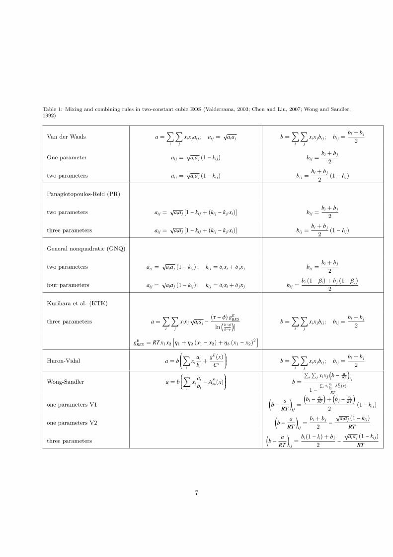
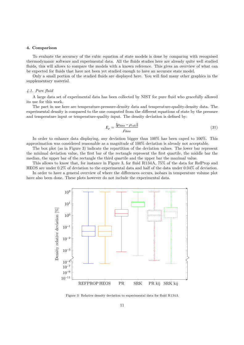
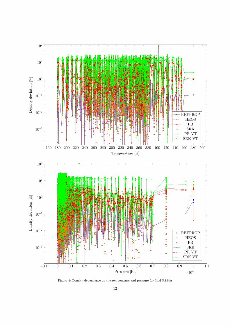
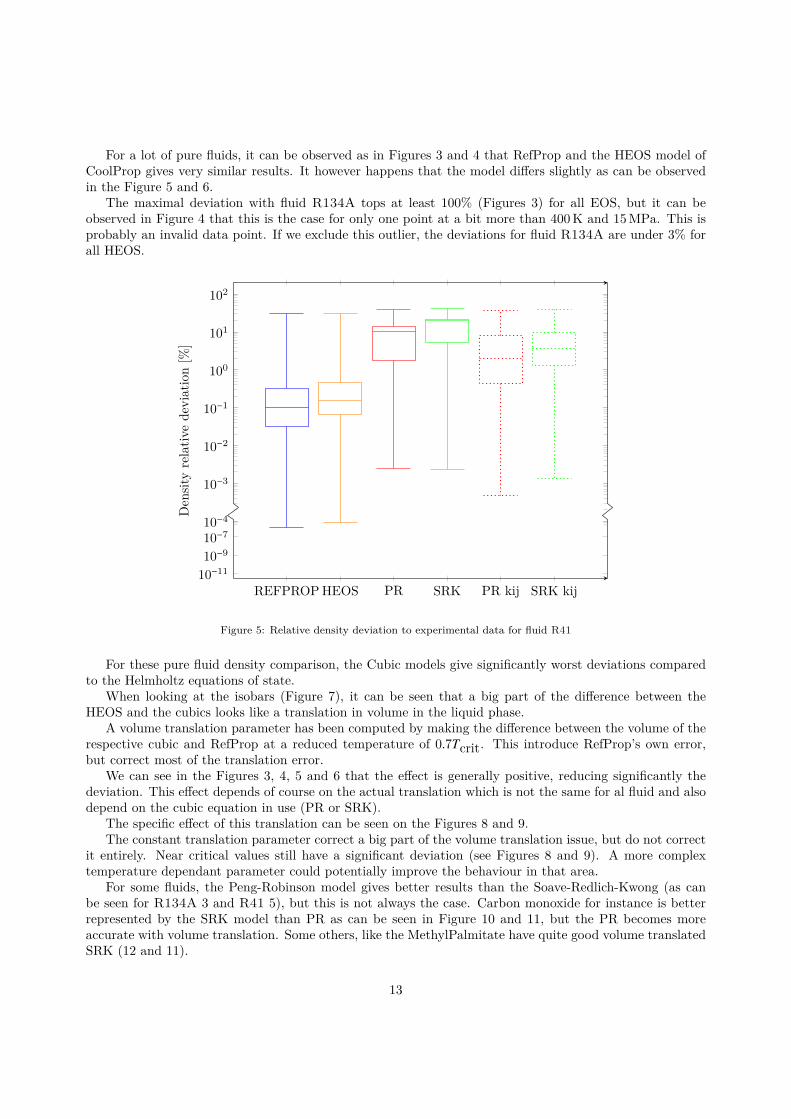
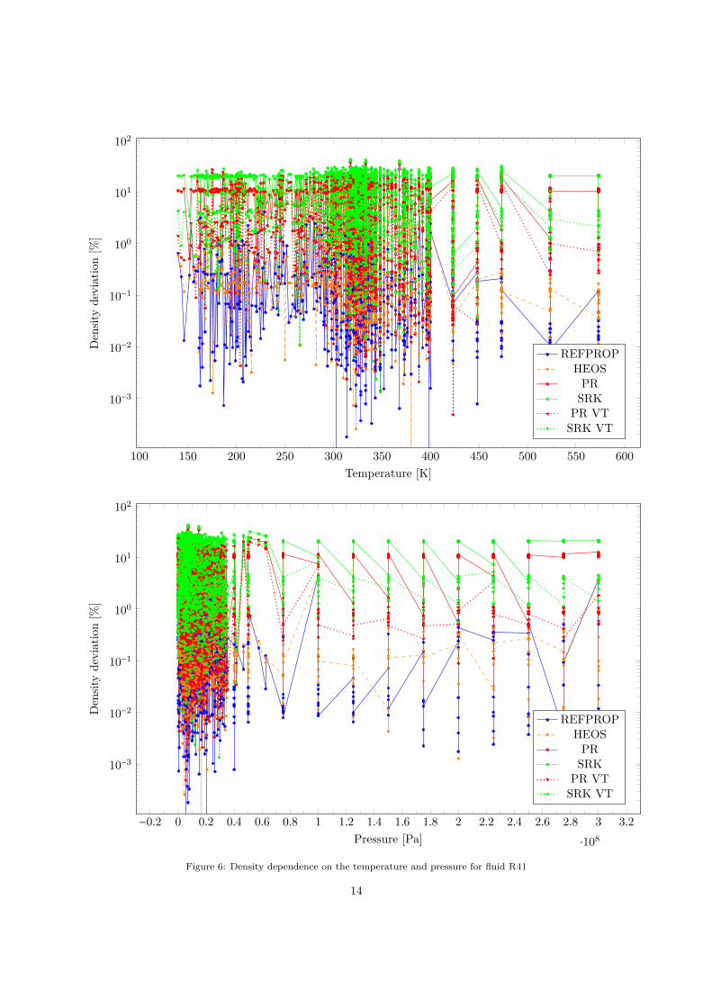
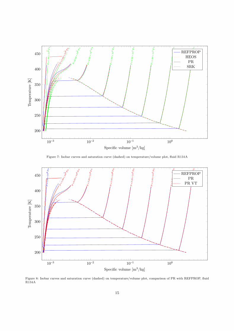
10minus3 10minus2 10minus1 100
200
250
300
350
400
450
P=
100times
104
Pa
P=
100times
104
Pa
P=
100times
104
Pa
P=
100times
104
Pa
P=
320times
104
Pa
P=
320times
104
Pa
P=
320times
104
Pa
P=
320times
104
Pa
P=
100times
105
Pa
P=
100times
105
Pa
P=
100times
105
Pa
P=
100times
105
Pa
P=
320times
105
Pa
P=
320times
105
Pa
P=
320times
105
Pa
P=
320times
105
Pa
P=
100times
106
Pa
P=
100times
106
Pa
P=
100times
106
Pa
P=
100times
106
Pa
P=
320times
106
Pa
P=
320times
106
Pa
P=
320times
106
Pa
P=
320times
106
Pa
P=
600times
106
Pa
P=
600times
106
Pa
P=
600times
106
Pa
P=
600times
106
Pa
P=
100times
107 P
a
P=
100times
107 P
a
P=
100times
107 P
a
P=
100times
107
Pa
P=
100times
108
Pa
P=
100times
108
Pa
P=
100times
108 P
a
P=
100times
108
Pa
Specific volume [m3kg]
Tem
pera
ture
[K]
REFPROPHEOS
PRSRK
Figure 7 Isobar curves and saturation curve (dashed) on temperaturevolume plot fluid R134A
10minus3 10minus2 10minus1 100
200
250
300
350
400
450
P=
100times
104
Pa
P=
100times
104
Pa
P=
100times
104
Pa
P=
320times
104
Pa
P=
320times
104
Pa
P=
320times
104
Pa
P=
100times
105
Pa
P=
100times
105
Pa
P=
100times
105
Pa
P=
320times
105
Pa
P=
320times
105
Pa
P=
320times
105
Pa
P=
100times
106
Pa
P=
100times
106
Pa
P=
100times
106
Pa
P=
320times
106
Pa
P=
320times
106
Pa
P=
320times
106
Pa
P=
600times
106
Pa
P=
600times
106
Pa
P=
600times
106
Pa
P=
100times
107 P
a
P=
100times
107 P
a
P=
100times
107 P
a
P=
100times
108
Pa
P=
100times
108 P
a
P=
100times
108 P
a
Specific volume [m3kg]
Tem
pera
ture
[K]
REFPROPPR
PR VT
Figure 8 Isobar curves and saturation curve (dashed) on temperaturevolume plot comparison of PR with REFPROP fluidR134A
15
10minus3 10minus2 10minus1 100
200
250
300
350
400
450
P=
100times
104
Pa
P=
100times
104
Pa
P=
100times
104
Pa
P=
320times
104
Pa
P=
320times
104
Pa
P=
320times
104
Pa
P=
100times
105
Pa
P=
100times
105
Pa
P=
100times
105
Pa
P=
320times
105
Pa
P=
320times
105
Pa
P=
320times
105
Pa
P=
100times
106
Pa
P=
100times
106
Pa
P=
100times
106
Pa
P=
320times
106
Pa
P=
320times
106
Pa
P=
320times
106
Pa
P=
600times
106
Pa
P=
600times
106
Pa
P=
600times
106
Pa
P=
100times
107 P
a
P=
100times
107
Pa
P=
100times
107
Pa
P=
100times
108
Pa
P=
100times
108
Pa
P=
100times
108
Pa
Specific volume [m3kg]
Tem
pera
ture
[K]
REFPROPSRK
SRK VT
Figure 9 Isobar curves and saturation curve (dashed) on temperaturevolume plot comparison of SRK with REFPROP fluidR134A
10minus4
10minus3
10minus2
10minus1
100
101
102
REFPROP HEOS PR SRK PR kij SRK kij10minus1110minus910minus7
Den
sity
rela
tive
devi
atio
n[
]
Figure 10 Relative density deviation to experimental data for fluid Carbon Monoxide
16
50 100 150 200 250 300 350 400 450 500 550 600
10minus3
10minus2
10minus1
100
101
102
Temperature [K]
Den
sity
devi
atio
n[
]
REFPROPHEOS
PRSRK
PR VTSRK VT
minus05 0 05 1 15 2 25 3 35 4 45 5 55 6 65
middot108
10minus3
10minus2
10minus1
100
101
102
Pressure [Pa]
Den
sity
devi
atio
n[
]
REFPROPHEOS
PRSRK
PR VTSRK VT
Figure 11 Density dependence on the temperature and pressure for fluid Carbon Monoxide
17
10minus4
10minus3
10minus2
10minus1
100
101
102
REFPROP HEOS PR SRK PR kij SRK kij10minus1110minus910minus7
Den
sity
rela
tive
devi
atio
n[
]
Figure 12 Relative density deviation to experimental data for fluid MethylPalmitate
It can also be noted that sometimes some EOS do not gives results when other ones gives or givesunacceptable deviations (ge 100) where others gives more reasonable results as for the fluid n-Dodecane(14 and 15)
In a general manner the relative deviations do not seem to be much affected by the temperature nor thepressure value 4 6 11 13 and 15 This means that the absolute deviation (the deviation in Pa or K) willincrease proportionally with the pressure and the temperature
18
310 320 330 340 350 360 370 380 390
10minus3
10minus2
10minus1
100
101
102
Temperature [K]
Den
sity
devi
atio
n[
]
REFPROPHEOS
PRSRK
PR VTSRK VT
minus05 0 05 1 15 2 25 3 35 4 45 5 55
middot107
10minus3
10minus2
10minus1
100
101
102
Pressure [Pa]
Den
sity
devi
atio
n[
]
REFPROPHEOS
PRSRK
PR VTSRK VT
Figure 13 Density dependence on the temperature and pressure for fluid MethylPalmitate
19
10minus4
10minus3
10minus2
10minus1
100
101
102
REFPROP HEOS PR SRK PR kij SRK kij10minus1110minus910minus7
Den
sity
rela
tive
devi
atio
n[
]
Figure 14 Relative density deviation to experimental data for fluid n-Dodecane
20
250 300 350 400 450 500 550 600 650
10minus3
10minus2
10minus1
100
101
102
Temperature [K]
Den
sity
devi
atio
n[
]
REFPROPHEOS
PRSRK
PR VTSRK VT
minus05 0 05 1 15 2 25 3 35 4 45 5 55 6 65 7 75
middot108
10minus3
10minus2
10minus1
100
101
102
Pressure [Pa]
Den
sity
devi
atio
n[
]
REFPROPHEOS
PRSRK
PR VTSRK VT
Figure 15 Density dependence on the temperature and pressure for fluid n-Dodecane
21
42 Binary mixturesAn other data set of experimental data has been collected by NIST for mixtures but only containing
vapour-liquid equilibrium (VLE) dataThese data consist of the molar fraction of each component and the temperature and pressure The
molar fraction at a given temperature and pressure are specified to be either liquid or gaseous which allowsto define the quality (0 or 1)
Two values where computed thanks to the state models the temperature from the pressure and thequality and the pressure from the temperature and quality The deviation between the computed valuesand the experimental data where then computed as following
ET =Tdata minus Tcalc
Tdata(32)
Ep =pdata minus pcalc
pdata(33)
The effect of the volume translation has not been evaluated here as no densityvolume data whereprovided
As these are mixtures there is the possibility to use an interaction parameter The one currentlyimplemented in CoolProp is the Van der Waals mixing rules with one parameter ki j For this work theinteraction parameter was fitted to minimize the deviation to experimental data with Brentrsquos method Theerror to minimise was expressed as follow
E =sum∣∣∣ET + 01Ep
∣∣∣ (34)
were ET and Ep are from equations 32 and 33The difference of results between pure temperature or pure pressure errors where not significant The
pressure term has been weighted by 01 as itrsquos magnitude was around 10 times bigger than the deviation interm of temperature
With the mixture the differences between RefProp and CoolProprsquos HEOS are a bit more marked as canbe seen in Figure 16 Depending on the fluid RefProp can be better than CoolProprsquos HEOS especiallywhen it comes to near critical data where the later tend to gives very wrong values (see Figure 18) but theFigure 19 is a good example where CoolProprsquos HEOS is far better
On the cubicrsquos side the results for the liquid-vapour equilibrium seems extremely good and comparablewith RefProp and CoolProprsquos HEOS It is interesting to notice that the volume translation problem occurringwith density and volume value do not seem to be a weight for these VLE data
A very important thing to notice with the mixture R1234YF-R134A is the influence of the molar fractionon the deviation (Figure 20) RefProp and the two cubics (without the binary interaction parameter ki j)have a deviation that considerable increases (around 10 times bigger) when mixing the two fluid comparedto the pure fluids with a maximum around equimolar composition This is the kind of behaviour that isexpected when using two sufficiently different fluids the way they interact together is different to the waythey interact with themselves
This effect is reduced with the interaction model and it appears that CoolProprsquos HEOS have a goodinteraction model for this mixture This is also corrected for the cubic by the ki j interaction parameterThis explains the better behaviour of CoolProprsquos HEOS and the cubics with interaction parameter for thisparticular mixture
Other mixtures like R134A-R32 are more similar and donrsquot benefit that much from a better mixing rule(Figure 17) This lead to more homogeneous deviations between the EOS
Again the variation of temperature and pressure on the relative deviation seems minimal except whenapproaching to the critical point
The temperature deviations are significantly smaller than the pressure deviations for all EOS
22
10minus4
10minus3
10minus2
10minus1
100
101
102
REFPROP HEOS PR SRK PR kij SRK kij10minus11
10minus9
10minus7Tem
pera
ture
rela
tive
devi
atio
n[
]
(a) Temperature deviation
10minus4
10minus3
10minus2
10minus1
100
101
102
REFPROP HEOS PR SRK PR kij SRK kij10minus11
10minus9
10minus7
Pres
sure
rela
tive
devi
atio
n[
]
(b) Pressure deviation
Figure 16 Relative deviation to experimental saturation data for mixtures based on R125 and R134A
23
0 01 02 03 04 05 06 07 08 09 110minus4
10minus3
10minus2
10minus1
100
Molar fraction of R134A [minus]
Tem
pera
ture
devi
atio
n[
]
REFPROPHEOS
PRSRK
PR ki jSRK ki j
0 01 02 03 04 05 06 07 08 09 110minus3
10minus2
10minus1
100
101
Molar fraction of R134A [minus]
Pres
sure
devi
atio
n[
]
REFPROPHEOS
PRSRK
PR ki jSRK ki j
Figure 17 Dependence on the molar fraction for the binary mixture R134A-R32
24
190 200 210 220 230 240 250 260 270 280 290 300 310 320 330 340 350 36010minus4
10minus3
10minus2
10minus1
100
Temperature [K]
Tem
pera
ture
devi
atio
n[
]
REFPROPHEOS
PRSRK
PR ki jSRK ki j
0 05 1 15 2 25 3 35 4
middot106
10minus3
10minus2
10minus1
100
101
Pressure [Pa]
Pres
sure
devi
atio
n[
]
REFPROPHEOS
PRSRK
PR ki jSRK ki j
Figure 18 Dependence on the temperature and pressure for the binary mixture R134A-R32
25
10minus4
10minus3
10minus2
10minus1
100
101
102
REFPROP HEOS PR SRK PR kij SRK kij10minus11
10minus9
10minus7Tem
pera
ture
rela
tive
devi
atio
n[
]
(a) Temperature deviation
10minus4
10minus3
10minus2
10minus1
100
101
102
REFPROP HEOS PR SRK PR kij SRK kij10minus11
10minus9
10minus7
Pres
sure
rela
tive
devi
atio
n[
]
(b) Pressure deviation
Figure 19 Relative deviation to experimental saturation data for mixtures based on R1234YF and R134A
26
0 01 02 03 04 05 06 07 08 09 110minus4
10minus3
10minus2
10minus1
100
Molar fraction of R1234YF [minus]
Tem
pera
ture
devi
atio
n[
]
REFPROPHEOS
PRSRK
PR ki jSRK ki j
0 01 02 03 04 05 06 07 08 09 110minus3
10minus2
10minus1
100
101
Molar fraction of R1234YF [minus]
Pres
sure
devi
atio
n[
]
REFPROPHEOS
PRSRK
PR ki jSRK ki j
Figure 20 Dependence on the molar fraction for the binary mixture R1234YF-R134A
27
270 275 280 285 290 295 300 305 310 315 320 325 330 335 34010minus4
10minus3
10minus2
10minus1
100
Temperature [K]
Tem
pera
ture
devi
atio
n[
]
REFPROPHEOS
PRSRK
PR ki jSRK ki j
02 03 04 05 06 07 08 09 1 11 12 13 14 15 16 17 18
middot106
10minus3
10minus2
10minus1
100
101
Pressure [Pa]
Pres
sure
devi
atio
n[
]
REFPROPHEOS
PRSRK
PR ki jSRK ki j
Figure 21 Dependence on the temperature and pressure for the binary mixture R1234YF-R134A
28
43 Ternary mixturesThe ternary mixtures are from the same data set as the binaries The binary interaction parameters ki j
where fitted with the binary mixture and reused hereThe results for the ternary mixtures are similar to the ones from the binaries
29
10minus4
10minus3
10minus2
10minus1
100
101
102
REFPROP HEOS PR SRK PR kij SRK kij10minus11
10minus9
10minus7Tem
pera
ture
rela
tive
devi
atio
n[
]
(a) Temperature deviation
10minus4
10minus3
10minus2
10minus1
100
101
102
REFPROP HEOS PR SRK PR kij SRK kij10minus11
10minus9
10minus7
Pres
sure
rela
tive
devi
atio
n[
]
(b) Pressure deviation
Figure 22 Relative deviation to experimental saturation data for mixtures based on R125 R32 and R134A
30
200 210 220 230 240 250 260 270 280 290 300 310 320 330 340 35010minus4
10minus3
10minus2
10minus1
100
Temperature [K]
Tem
pera
ture
devi
atio
n[
]
REFPROPHEOS
PRSRK
PR ki jSRK ki j
minus02 0 02 04 06 08 1 12 14 16 18 2 22 24 26 28 3 32 34 36 38
middot106
10minus3
10minus2
10minus1
100
101
Pressure [Pa]
Pres
sure
devi
atio
n[
]
REFPROPHEOS
PRSRK
PR ki jSRK ki j
Figure 23 Dependence on the temperature and pressure for the ternary mixture R125-R32-R134A
31
5 Acknowledgements
I would like to thank the professor Sylvain Quoilin for having given to me the opportunity to make thismaster thesis abroad This was a very interesting experience which allowed me to practice English and meetan other culture
I have a big thank to give to the DTU team who took care of me in Denmark the professor FredrikHaglind and the two post doctorates Maria E Mondejar Montagud and Jorrit Wronski It was a realpleasure to work with them
I also thanks Ian Bell our contact at NIST who manage to provide us with the database and withoutwho CoolProp would not exist
32
6 Conclusions
The simple cubic equations of state do not always gives satisfying results to compute density This canhowever be mostly corrected with a simple translation coefficient requiring a single measurement of saturatedliquid and more complex translation models could potentially give more accurate results
The cubic equations of states are very effective at modelling the liquid vapour equilibrium competingwith well recognise software
Depending on the interaction between the fluid constituting the mixtures all models benefit from binaryinteraction knowledge This is sometimes integrated in the software but would generally be an issue withnot yet well studied mixtures A simple coefficient (to be determined experimentally or approximated) canbe used to improve greatly the results of cubic equations when the interaction between the fluids is signif-icant An alternative would be to approximate the interaction with the UNIFAQ model as it is done withthe VTPR Determination of models to approximate the binary interaction parameters depending on thetype of fluid used would be an interesting subject for complementary study
More complex models can be used for the attractive parameter like the Mathias-Copeman and the TWUequations They both require 3 supplementary parameters and are already implemented in CoolProp Theirimpact could be interesting for a further study
The speed of the models are not compared in this work The comparison would be interesting butit is useful to notice CoolProp also provide a tabular interface which allows for extremely fast propertiescomputation when the tables have been generated (with a small loss of accuracy)
The cubic equations of states gives a wide range of possibilities from the simplest and fast model butslightly lacking accuracy to more complex and accurate models They provide a great tool for evaluation offluids when few data are available
33
Ahlers J Gmehling J 2001 Development of an universal group contribution equation of state Prediction of liquid densitiesfor pure compounds with a volume translated Peng-Robinson equation of state Fluid Phase Equilibria 191 (1-2) 177ndash188URL httpwwwsciencedirectcomsciencearticlepiiS0378381201006264pdfftmd5=86daea9e53bace87587e62b056b3007eamppid=1-s20-S0378381201006264-mainpdf
Bell I Jaumlger A 2016a Helmholtz energy transformation of common cubic equations of state for use with pure fluids andmixtures Journal of Research of the National Institute of Standards and Technology 121 (July) 238ndash263URL httpswwwresearchgatenetpublication304186500_Helmholtz_Energy_Transformations_of_Common_Cubic_Equations_of_State_for_Use_with_Pure_Fluids_and_Mixtures
Bell I H Jaumlger A 2016b Intermediate Terms 1ndash14Bell I H Jaumlger A 2016c Supplementary Information to accompany Helmholtz energy transformations of common cubic
equations of state for use with pure fluids and mixtures No 5Chen W-Y Liu J 2007 Mathcad Modules for Supercritical Fluid Extraction based on Mixing Rules Appendix A - Mixing
Rules (662) 1ndash10URL httphomeolemissedu~cmchengsExtractionAppendixA_MixingRulesdoc
CoolProp 2016 Cubic Equations of StateURL httpwwwcoolproporgcoolpropCubicshtml
Fauacutendez C a Valderrama J O 2009 Low pressure vaporndashliquid equilibrium in ethanol+congener mixtures using theWongndashSandler mixing rule Thermochimica Acta 490 (1-2) 37ndash42URL httpwwwsciencedirectcomsciencearticlepiiS0040603109000999pdfftmd5=65533f85d53569eeebae29e565402cc4amppid=1-s20-S0040603109000999-mainpdf
Frey K Augustine C Ciccolini R P Paap S Modell M Tester J 2007 Volume translation in equations of state as ameans of accurate property estimation Fluid Phase Equilibria 260 (2) 316ndash325URL httpwwwsciencedirectcomsciencearticlepiiS0378381207004591pdfftmd5=c750d4ea93f662a13b87183c76a8654eamppid=1-s20-S0378381207004591-mainpdf
Ji W-R Lempe D 1997 Density improvement of the SRK equation of state Fluid Phase Equilibria 130 (1-2) 49ndash63URL httpwwwsciencedirectcomsciencearticlepiiS0378381296031901
Lemmon E W Huber M L McLinden M O 2013 Reference Fluid Thermodynamic and Transport Properties-REFPROPversion 91URL httpwwwnistgovsrduploadREFPROP9PDF
Loacutepez J A Cardona C A 2006 Phase equilibrium calculations for carbon dioxide+n-alkanes binary mixtures with theWongndashSandler mixing rules Fluid Phase Equilibria 239 (2) 206ndash212URL httpwwwsciencedirectcomsciencearticlepiiS0378381205004565
Martin J J 1967 Equations of StatemdashApplied Thermodynamics Symposium Industrial amp Engineering Chemistry 59 (12)34ndash52URL httpdxdoiorg101021ie50696a008$delimiter026E30F$nhttppubsacsorgdoipdf101021ie50696a008
Martin J J 1979 Cubic Equations of State-Which Industrial amp Engineering Chemistry Fundamentals 18 (2) 81ndash97URL httpdxdoiorg101021i160070a001
Meng L Duan Y Y Wang X D 2007 Binary interaction parameter kij for calculating the second cross-virial coefficientsof mixtures Fluid Phase Equilibria 260 (2) 354ndash358URL httpwwwsciencedirectcomsciencearticlepiiS0378381207004323pdfftmd5=e3b19d08e08099003d28392a4450f768amppid=1-s20-S0378381207004323-mainpdf
Peng D-Y Robinson D B 1976 A New Two-Constant Equation of State Industrial amp Engineering Chemistry Fundamentals15 (1) 59ndash64URL httppubsacsorgdoiabs101021i160057a011
Schmid B Gmehling J 2012 Revised parameters and typical results of the VTPR group contribution equation of stateFluid Phase Equilibria 317 110ndash126URL httpdxdoiorg101016jfluid201201006
Schmid B Schedemann A Gmehling J 2014 Extension of the VTPR group contribution equation of state Groupinteraction parameters for additional 192 group combinations and typical results Industrial and Engineering ChemistryResearch 53 (8) 3393ndash3405
Soave G 1972 Equilibrium constants from a modified Redlich-Kwong equation of state Chemical Engineering Science 27 (6)1197ndash1203URL httpacels-cdncom00092509728009641-s20-0009250972800964-mainpdf_tid=cd3fc6c8-1dbd-11e6-a8de-00000aacb35dampacdnat=1463661351_8f1dbe034b52854e2d97cd6d80b7b56b
Valderrama J O 2003 The State of the Cubic Equations of State Industrial amp Engineering Chemistry Research 42 (8)1603ndash1618URL httppubsacsorgdoiabs101021ie020447b
Valderrama J O Marambio L E Silva A a 2002 Mixing rules in cubic equations of state applied to refrigerant mixturesJournal of Phase Equilibria 23 (6) 495ndash501URL httpdownloadspringercomstaticpdf558art3A1013612F105497102770331181pdforiginUrl=httplinkspringercomarticle101361105497102770331181amptoken2=exp=1463652668~acl=staticpdf558art253A101361252F105497102770
Wong D S H Sandler S I 1992 A Theoretically Correct Mixing Rule for Cubic Equations of State 38 (5)URL httponlinelibrarywileycomdoi101002aic690380505epdf
34
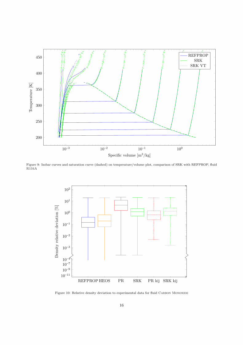
10minus3 10minus2 10minus1 100
200
250
300
350
400
450
P=
100times
104
Pa
P=
100times
104
Pa
P=
100times
104
Pa
P=
320times
104
Pa
P=
320times
104
Pa
P=
320times
104
Pa
P=
100times
105
Pa
P=
100times
105
Pa
P=
100times
105
Pa
P=
320times
105
Pa
P=
320times
105
Pa
P=
320times
105
Pa
P=
100times
106
Pa
P=
100times
106
Pa
P=
100times
106
Pa
P=
320times
106
Pa
P=
320times
106
Pa
P=
320times
106
Pa
P=
600times
106
Pa
P=
600times
106
Pa
P=
600times
106
Pa
P=
100times
107 P
a
P=
100times
107
Pa
P=
100times
107
Pa
P=
100times
108
Pa
P=
100times
108
Pa
P=
100times
108
Pa
Specific volume [m3kg]
Tem
pera
ture
[K]
REFPROPSRK
SRK VT
Figure 9 Isobar curves and saturation curve (dashed) on temperaturevolume plot comparison of SRK with REFPROP fluidR134A
10minus4
10minus3
10minus2
10minus1
100
101
102
REFPROP HEOS PR SRK PR kij SRK kij10minus1110minus910minus7
Den
sity
rela
tive
devi
atio
n[
]
Figure 10 Relative density deviation to experimental data for fluid Carbon Monoxide
16
50 100 150 200 250 300 350 400 450 500 550 600
10minus3
10minus2
10minus1
100
101
102
Temperature [K]
Den
sity
devi
atio
n[
]
REFPROPHEOS
PRSRK
PR VTSRK VT
minus05 0 05 1 15 2 25 3 35 4 45 5 55 6 65
middot108
10minus3
10minus2
10minus1
100
101
102
Pressure [Pa]
Den
sity
devi
atio
n[
]
REFPROPHEOS
PRSRK
PR VTSRK VT
Figure 11 Density dependence on the temperature and pressure for fluid Carbon Monoxide
17
10minus4
10minus3
10minus2
10minus1
100
101
102
REFPROP HEOS PR SRK PR kij SRK kij10minus1110minus910minus7
Den
sity
rela
tive
devi
atio
n[
]
Figure 12 Relative density deviation to experimental data for fluid MethylPalmitate
It can also be noted that sometimes some EOS do not gives results when other ones gives or givesunacceptable deviations (ge 100) where others gives more reasonable results as for the fluid n-Dodecane(14 and 15)
In a general manner the relative deviations do not seem to be much affected by the temperature nor thepressure value 4 6 11 13 and 15 This means that the absolute deviation (the deviation in Pa or K) willincrease proportionally with the pressure and the temperature
18
310 320 330 340 350 360 370 380 390
10minus3
10minus2
10minus1
100
101
102
Temperature [K]
Den
sity
devi
atio
n[
]
REFPROPHEOS
PRSRK
PR VTSRK VT
minus05 0 05 1 15 2 25 3 35 4 45 5 55
middot107
10minus3
10minus2
10minus1
100
101
102
Pressure [Pa]
Den
sity
devi
atio
n[
]
REFPROPHEOS
PRSRK
PR VTSRK VT
Figure 13 Density dependence on the temperature and pressure for fluid MethylPalmitate
19
10minus4
10minus3
10minus2
10minus1
100
101
102
REFPROP HEOS PR SRK PR kij SRK kij10minus1110minus910minus7
Den
sity
rela
tive
devi
atio
n[
]
Figure 14 Relative density deviation to experimental data for fluid n-Dodecane
20
250 300 350 400 450 500 550 600 650
10minus3
10minus2
10minus1
100
101
102
Temperature [K]
Den
sity
devi
atio
n[
]
REFPROPHEOS
PRSRK
PR VTSRK VT
minus05 0 05 1 15 2 25 3 35 4 45 5 55 6 65 7 75
middot108
10minus3
10minus2
10minus1
100
101
102
Pressure [Pa]
Den
sity
devi
atio
n[
]
REFPROPHEOS
PRSRK
PR VTSRK VT
Figure 15 Density dependence on the temperature and pressure for fluid n-Dodecane
21
42 Binary mixturesAn other data set of experimental data has been collected by NIST for mixtures but only containing
vapour-liquid equilibrium (VLE) dataThese data consist of the molar fraction of each component and the temperature and pressure The
molar fraction at a given temperature and pressure are specified to be either liquid or gaseous which allowsto define the quality (0 or 1)
Two values where computed thanks to the state models the temperature from the pressure and thequality and the pressure from the temperature and quality The deviation between the computed valuesand the experimental data where then computed as following
ET =Tdata minus Tcalc
Tdata(32)
Ep =pdata minus pcalc
pdata(33)
The effect of the volume translation has not been evaluated here as no densityvolume data whereprovided
As these are mixtures there is the possibility to use an interaction parameter The one currentlyimplemented in CoolProp is the Van der Waals mixing rules with one parameter ki j For this work theinteraction parameter was fitted to minimize the deviation to experimental data with Brentrsquos method Theerror to minimise was expressed as follow
E =sum∣∣∣ET + 01Ep
∣∣∣ (34)
were ET and Ep are from equations 32 and 33The difference of results between pure temperature or pure pressure errors where not significant The
pressure term has been weighted by 01 as itrsquos magnitude was around 10 times bigger than the deviation interm of temperature
With the mixture the differences between RefProp and CoolProprsquos HEOS are a bit more marked as canbe seen in Figure 16 Depending on the fluid RefProp can be better than CoolProprsquos HEOS especiallywhen it comes to near critical data where the later tend to gives very wrong values (see Figure 18) but theFigure 19 is a good example where CoolProprsquos HEOS is far better
On the cubicrsquos side the results for the liquid-vapour equilibrium seems extremely good and comparablewith RefProp and CoolProprsquos HEOS It is interesting to notice that the volume translation problem occurringwith density and volume value do not seem to be a weight for these VLE data
A very important thing to notice with the mixture R1234YF-R134A is the influence of the molar fractionon the deviation (Figure 20) RefProp and the two cubics (without the binary interaction parameter ki j)have a deviation that considerable increases (around 10 times bigger) when mixing the two fluid comparedto the pure fluids with a maximum around equimolar composition This is the kind of behaviour that isexpected when using two sufficiently different fluids the way they interact together is different to the waythey interact with themselves
This effect is reduced with the interaction model and it appears that CoolProprsquos HEOS have a goodinteraction model for this mixture This is also corrected for the cubic by the ki j interaction parameterThis explains the better behaviour of CoolProprsquos HEOS and the cubics with interaction parameter for thisparticular mixture
Other mixtures like R134A-R32 are more similar and donrsquot benefit that much from a better mixing rule(Figure 17) This lead to more homogeneous deviations between the EOS
Again the variation of temperature and pressure on the relative deviation seems minimal except whenapproaching to the critical point
The temperature deviations are significantly smaller than the pressure deviations for all EOS
22
10minus4
10minus3
10minus2
10minus1
100
101
102
REFPROP HEOS PR SRK PR kij SRK kij10minus11
10minus9
10minus7Tem
pera
ture
rela
tive
devi
atio
n[
]
(a) Temperature deviation
10minus4
10minus3
10minus2
10minus1
100
101
102
REFPROP HEOS PR SRK PR kij SRK kij10minus11
10minus9
10minus7
Pres
sure
rela
tive
devi
atio
n[
]
(b) Pressure deviation
Figure 16 Relative deviation to experimental saturation data for mixtures based on R125 and R134A
23
0 01 02 03 04 05 06 07 08 09 110minus4
10minus3
10minus2
10minus1
100
Molar fraction of R134A [minus]
Tem
pera
ture
devi
atio
n[
]
REFPROPHEOS
PRSRK
PR ki jSRK ki j
0 01 02 03 04 05 06 07 08 09 110minus3
10minus2
10minus1
100
101
Molar fraction of R134A [minus]
Pres
sure
devi
atio
n[
]
REFPROPHEOS
PRSRK
PR ki jSRK ki j
Figure 17 Dependence on the molar fraction for the binary mixture R134A-R32
24
190 200 210 220 230 240 250 260 270 280 290 300 310 320 330 340 350 36010minus4
10minus3
10minus2
10minus1
100
Temperature [K]
Tem
pera
ture
devi
atio
n[
]
REFPROPHEOS
PRSRK
PR ki jSRK ki j
0 05 1 15 2 25 3 35 4
middot106
10minus3
10minus2
10minus1
100
101
Pressure [Pa]
Pres
sure
devi
atio
n[
]
REFPROPHEOS
PRSRK
PR ki jSRK ki j
Figure 18 Dependence on the temperature and pressure for the binary mixture R134A-R32
25
10minus4
10minus3
10minus2
10minus1
100
101
102
REFPROP HEOS PR SRK PR kij SRK kij10minus11
10minus9
10minus7Tem
pera
ture
rela
tive
devi
atio
n[
]
(a) Temperature deviation
10minus4
10minus3
10minus2
10minus1
100
101
102
REFPROP HEOS PR SRK PR kij SRK kij10minus11
10minus9
10minus7
Pres
sure
rela
tive
devi
atio
n[
]
(b) Pressure deviation
Figure 19 Relative deviation to experimental saturation data for mixtures based on R1234YF and R134A
26
0 01 02 03 04 05 06 07 08 09 110minus4
10minus3
10minus2
10minus1
100
Molar fraction of R1234YF [minus]
Tem
pera
ture
devi
atio
n[
]
REFPROPHEOS
PRSRK
PR ki jSRK ki j
0 01 02 03 04 05 06 07 08 09 110minus3
10minus2
10minus1
100
101
Molar fraction of R1234YF [minus]
Pres
sure
devi
atio
n[
]
REFPROPHEOS
PRSRK
PR ki jSRK ki j
Figure 20 Dependence on the molar fraction for the binary mixture R1234YF-R134A
27
270 275 280 285 290 295 300 305 310 315 320 325 330 335 34010minus4
10minus3
10minus2
10minus1
100
Temperature [K]
Tem
pera
ture
devi
atio
n[
]
REFPROPHEOS
PRSRK
PR ki jSRK ki j
02 03 04 05 06 07 08 09 1 11 12 13 14 15 16 17 18
middot106
10minus3
10minus2
10minus1
100
101
Pressure [Pa]
Pres
sure
devi
atio
n[
]
REFPROPHEOS
PRSRK
PR ki jSRK ki j
Figure 21 Dependence on the temperature and pressure for the binary mixture R1234YF-R134A
28
43 Ternary mixturesThe ternary mixtures are from the same data set as the binaries The binary interaction parameters ki j
where fitted with the binary mixture and reused hereThe results for the ternary mixtures are similar to the ones from the binaries
29
10minus4
10minus3
10minus2
10minus1
100
101
102
REFPROP HEOS PR SRK PR kij SRK kij10minus11
10minus9
10minus7Tem
pera
ture
rela
tive
devi
atio
n[
]
(a) Temperature deviation
10minus4
10minus3
10minus2
10minus1
100
101
102
REFPROP HEOS PR SRK PR kij SRK kij10minus11
10minus9
10minus7
Pres
sure
rela
tive
devi
atio
n[
]
(b) Pressure deviation
Figure 22 Relative deviation to experimental saturation data for mixtures based on R125 R32 and R134A
30
200 210 220 230 240 250 260 270 280 290 300 310 320 330 340 35010minus4
10minus3
10minus2
10minus1
100
Temperature [K]
Tem
pera
ture
devi
atio
n[
]
REFPROPHEOS
PRSRK
PR ki jSRK ki j
minus02 0 02 04 06 08 1 12 14 16 18 2 22 24 26 28 3 32 34 36 38
middot106
10minus3
10minus2
10minus1
100
101
Pressure [Pa]
Pres
sure
devi
atio
n[
]
REFPROPHEOS
PRSRK
PR ki jSRK ki j
Figure 23 Dependence on the temperature and pressure for the ternary mixture R125-R32-R134A
31
5 Acknowledgements
I would like to thank the professor Sylvain Quoilin for having given to me the opportunity to make thismaster thesis abroad This was a very interesting experience which allowed me to practice English and meetan other culture
I have a big thank to give to the DTU team who took care of me in Denmark the professor FredrikHaglind and the two post doctorates Maria E Mondejar Montagud and Jorrit Wronski It was a realpleasure to work with them
I also thanks Ian Bell our contact at NIST who manage to provide us with the database and withoutwho CoolProp would not exist
32
6 Conclusions
The simple cubic equations of state do not always gives satisfying results to compute density This canhowever be mostly corrected with a simple translation coefficient requiring a single measurement of saturatedliquid and more complex translation models could potentially give more accurate results
The cubic equations of states are very effective at modelling the liquid vapour equilibrium competingwith well recognise software
Depending on the interaction between the fluid constituting the mixtures all models benefit from binaryinteraction knowledge This is sometimes integrated in the software but would generally be an issue withnot yet well studied mixtures A simple coefficient (to be determined experimentally or approximated) canbe used to improve greatly the results of cubic equations when the interaction between the fluids is signif-icant An alternative would be to approximate the interaction with the UNIFAQ model as it is done withthe VTPR Determination of models to approximate the binary interaction parameters depending on thetype of fluid used would be an interesting subject for complementary study
More complex models can be used for the attractive parameter like the Mathias-Copeman and the TWUequations They both require 3 supplementary parameters and are already implemented in CoolProp Theirimpact could be interesting for a further study
The speed of the models are not compared in this work The comparison would be interesting butit is useful to notice CoolProp also provide a tabular interface which allows for extremely fast propertiescomputation when the tables have been generated (with a small loss of accuracy)
The cubic equations of states gives a wide range of possibilities from the simplest and fast model butslightly lacking accuracy to more complex and accurate models They provide a great tool for evaluation offluids when few data are available
33
Ahlers J Gmehling J 2001 Development of an universal group contribution equation of state Prediction of liquid densitiesfor pure compounds with a volume translated Peng-Robinson equation of state Fluid Phase Equilibria 191 (1-2) 177ndash188URL httpwwwsciencedirectcomsciencearticlepiiS0378381201006264pdfftmd5=86daea9e53bace87587e62b056b3007eamppid=1-s20-S0378381201006264-mainpdf
Bell I Jaumlger A 2016a Helmholtz energy transformation of common cubic equations of state for use with pure fluids andmixtures Journal of Research of the National Institute of Standards and Technology 121 (July) 238ndash263URL httpswwwresearchgatenetpublication304186500_Helmholtz_Energy_Transformations_of_Common_Cubic_Equations_of_State_for_Use_with_Pure_Fluids_and_Mixtures
Bell I H Jaumlger A 2016b Intermediate Terms 1ndash14Bell I H Jaumlger A 2016c Supplementary Information to accompany Helmholtz energy transformations of common cubic
equations of state for use with pure fluids and mixtures No 5Chen W-Y Liu J 2007 Mathcad Modules for Supercritical Fluid Extraction based on Mixing Rules Appendix A - Mixing
Rules (662) 1ndash10URL httphomeolemissedu~cmchengsExtractionAppendixA_MixingRulesdoc
CoolProp 2016 Cubic Equations of StateURL httpwwwcoolproporgcoolpropCubicshtml
Fauacutendez C a Valderrama J O 2009 Low pressure vaporndashliquid equilibrium in ethanol+congener mixtures using theWongndashSandler mixing rule Thermochimica Acta 490 (1-2) 37ndash42URL httpwwwsciencedirectcomsciencearticlepiiS0040603109000999pdfftmd5=65533f85d53569eeebae29e565402cc4amppid=1-s20-S0040603109000999-mainpdf
Frey K Augustine C Ciccolini R P Paap S Modell M Tester J 2007 Volume translation in equations of state as ameans of accurate property estimation Fluid Phase Equilibria 260 (2) 316ndash325URL httpwwwsciencedirectcomsciencearticlepiiS0378381207004591pdfftmd5=c750d4ea93f662a13b87183c76a8654eamppid=1-s20-S0378381207004591-mainpdf
Ji W-R Lempe D 1997 Density improvement of the SRK equation of state Fluid Phase Equilibria 130 (1-2) 49ndash63URL httpwwwsciencedirectcomsciencearticlepiiS0378381296031901
Lemmon E W Huber M L McLinden M O 2013 Reference Fluid Thermodynamic and Transport Properties-REFPROPversion 91URL httpwwwnistgovsrduploadREFPROP9PDF
Loacutepez J A Cardona C A 2006 Phase equilibrium calculations for carbon dioxide+n-alkanes binary mixtures with theWongndashSandler mixing rules Fluid Phase Equilibria 239 (2) 206ndash212URL httpwwwsciencedirectcomsciencearticlepiiS0378381205004565
Martin J J 1967 Equations of StatemdashApplied Thermodynamics Symposium Industrial amp Engineering Chemistry 59 (12)34ndash52URL httpdxdoiorg101021ie50696a008$delimiter026E30F$nhttppubsacsorgdoipdf101021ie50696a008
Martin J J 1979 Cubic Equations of State-Which Industrial amp Engineering Chemistry Fundamentals 18 (2) 81ndash97URL httpdxdoiorg101021i160070a001
Meng L Duan Y Y Wang X D 2007 Binary interaction parameter kij for calculating the second cross-virial coefficientsof mixtures Fluid Phase Equilibria 260 (2) 354ndash358URL httpwwwsciencedirectcomsciencearticlepiiS0378381207004323pdfftmd5=e3b19d08e08099003d28392a4450f768amppid=1-s20-S0378381207004323-mainpdf
Peng D-Y Robinson D B 1976 A New Two-Constant Equation of State Industrial amp Engineering Chemistry Fundamentals15 (1) 59ndash64URL httppubsacsorgdoiabs101021i160057a011
Schmid B Gmehling J 2012 Revised parameters and typical results of the VTPR group contribution equation of stateFluid Phase Equilibria 317 110ndash126URL httpdxdoiorg101016jfluid201201006
Schmid B Schedemann A Gmehling J 2014 Extension of the VTPR group contribution equation of state Groupinteraction parameters for additional 192 group combinations and typical results Industrial and Engineering ChemistryResearch 53 (8) 3393ndash3405
Soave G 1972 Equilibrium constants from a modified Redlich-Kwong equation of state Chemical Engineering Science 27 (6)1197ndash1203URL httpacels-cdncom00092509728009641-s20-0009250972800964-mainpdf_tid=cd3fc6c8-1dbd-11e6-a8de-00000aacb35dampacdnat=1463661351_8f1dbe034b52854e2d97cd6d80b7b56b
Valderrama J O 2003 The State of the Cubic Equations of State Industrial amp Engineering Chemistry Research 42 (8)1603ndash1618URL httppubsacsorgdoiabs101021ie020447b
Valderrama J O Marambio L E Silva A a 2002 Mixing rules in cubic equations of state applied to refrigerant mixturesJournal of Phase Equilibria 23 (6) 495ndash501URL httpdownloadspringercomstaticpdf558art3A1013612F105497102770331181pdforiginUrl=httplinkspringercomarticle101361105497102770331181amptoken2=exp=1463652668~acl=staticpdf558art253A101361252F105497102770
Wong D S H Sandler S I 1992 A Theoretically Correct Mixing Rule for Cubic Equations of State 38 (5)URL httponlinelibrarywileycomdoi101002aic690380505epdf
34
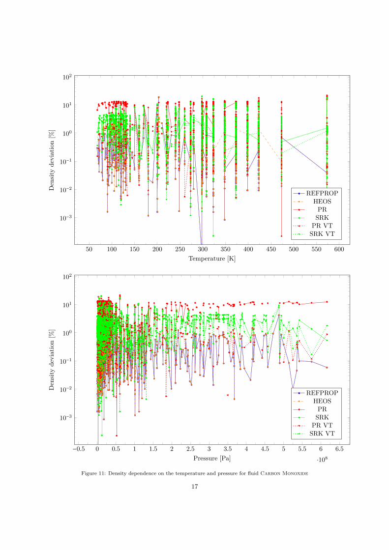
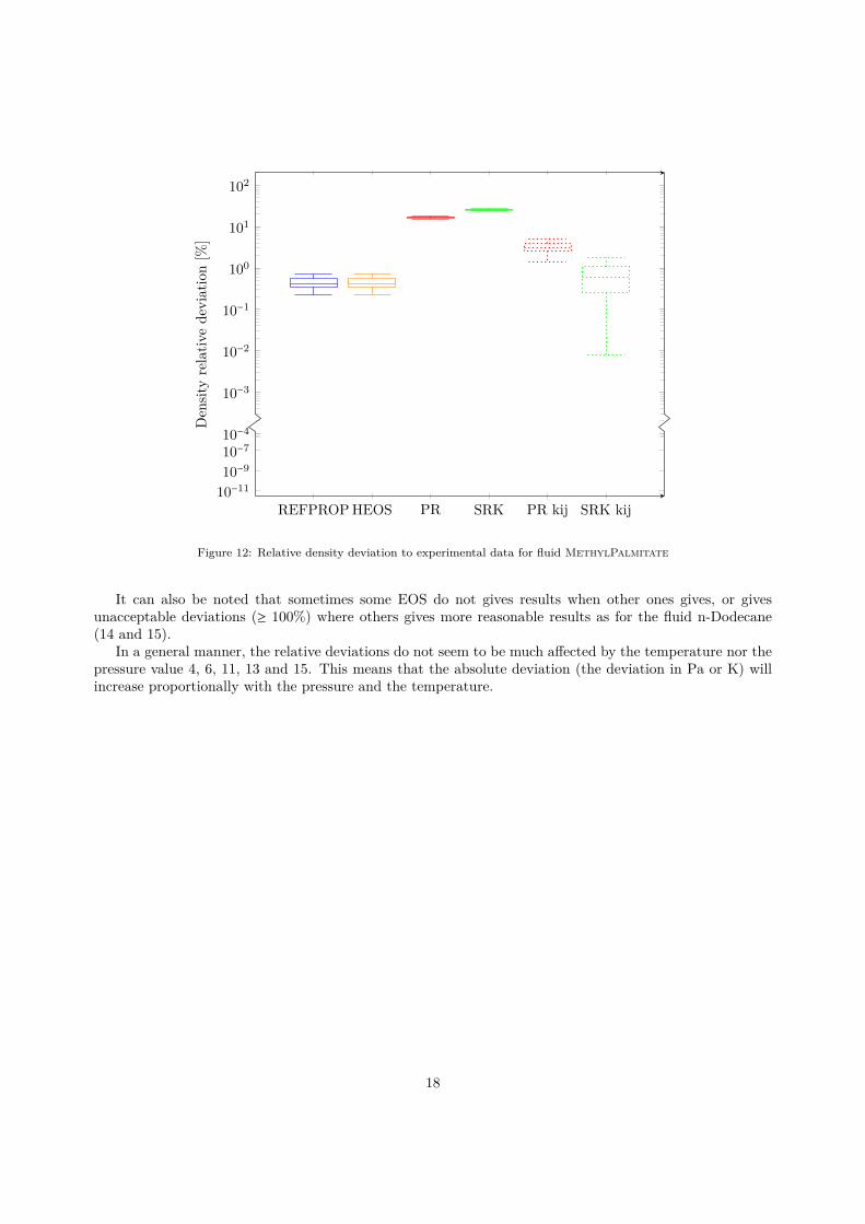
10minus4
10minus3
10minus2
10minus1
100
101
102
REFPROP HEOS PR SRK PR kij SRK kij10minus1110minus910minus7
Den
sity
rela
tive
devi
atio
n[
]
Figure 12 Relative density deviation to experimental data for fluid MethylPalmitate
It can also be noted that sometimes some EOS do not gives results when other ones gives or givesunacceptable deviations (ge 100) where others gives more reasonable results as for the fluid n-Dodecane(14 and 15)
In a general manner the relative deviations do not seem to be much affected by the temperature nor thepressure value 4 6 11 13 and 15 This means that the absolute deviation (the deviation in Pa or K) willincrease proportionally with the pressure and the temperature
18
310 320 330 340 350 360 370 380 390
10minus3
10minus2
10minus1
100
101
102
Temperature [K]
Den
sity
devi
atio
n[
]
REFPROPHEOS
PRSRK
PR VTSRK VT
minus05 0 05 1 15 2 25 3 35 4 45 5 55
middot107
10minus3
10minus2
10minus1
100
101
102
Pressure [Pa]
Den
sity
devi
atio
n[
]
REFPROPHEOS
PRSRK
PR VTSRK VT
Figure 13 Density dependence on the temperature and pressure for fluid MethylPalmitate
19
10minus4
10minus3
10minus2
10minus1
100
101
102
REFPROP HEOS PR SRK PR kij SRK kij10minus1110minus910minus7
Den
sity
rela
tive
devi
atio
n[
]
Figure 14 Relative density deviation to experimental data for fluid n-Dodecane
20
250 300 350 400 450 500 550 600 650
10minus3
10minus2
10minus1
100
101
102
Temperature [K]
Den
sity
devi
atio
n[
]
REFPROPHEOS
PRSRK
PR VTSRK VT
minus05 0 05 1 15 2 25 3 35 4 45 5 55 6 65 7 75
middot108
10minus3
10minus2
10minus1
100
101
102
Pressure [Pa]
Den
sity
devi
atio
n[
]
REFPROPHEOS
PRSRK
PR VTSRK VT
Figure 15 Density dependence on the temperature and pressure for fluid n-Dodecane
21
42 Binary mixturesAn other data set of experimental data has been collected by NIST for mixtures but only containing
vapour-liquid equilibrium (VLE) dataThese data consist of the molar fraction of each component and the temperature and pressure The
molar fraction at a given temperature and pressure are specified to be either liquid or gaseous which allowsto define the quality (0 or 1)
Two values where computed thanks to the state models the temperature from the pressure and thequality and the pressure from the temperature and quality The deviation between the computed valuesand the experimental data where then computed as following
ET =Tdata minus Tcalc
Tdata(32)
Ep =pdata minus pcalc
pdata(33)
The effect of the volume translation has not been evaluated here as no densityvolume data whereprovided
As these are mixtures there is the possibility to use an interaction parameter The one currentlyimplemented in CoolProp is the Van der Waals mixing rules with one parameter ki j For this work theinteraction parameter was fitted to minimize the deviation to experimental data with Brentrsquos method Theerror to minimise was expressed as follow
E =sum∣∣∣ET + 01Ep
∣∣∣ (34)
were ET and Ep are from equations 32 and 33The difference of results between pure temperature or pure pressure errors where not significant The
pressure term has been weighted by 01 as itrsquos magnitude was around 10 times bigger than the deviation interm of temperature
With the mixture the differences between RefProp and CoolProprsquos HEOS are a bit more marked as canbe seen in Figure 16 Depending on the fluid RefProp can be better than CoolProprsquos HEOS especiallywhen it comes to near critical data where the later tend to gives very wrong values (see Figure 18) but theFigure 19 is a good example where CoolProprsquos HEOS is far better
On the cubicrsquos side the results for the liquid-vapour equilibrium seems extremely good and comparablewith RefProp and CoolProprsquos HEOS It is interesting to notice that the volume translation problem occurringwith density and volume value do not seem to be a weight for these VLE data
A very important thing to notice with the mixture R1234YF-R134A is the influence of the molar fractionon the deviation (Figure 20) RefProp and the two cubics (without the binary interaction parameter ki j)have a deviation that considerable increases (around 10 times bigger) when mixing the two fluid comparedto the pure fluids with a maximum around equimolar composition This is the kind of behaviour that isexpected when using two sufficiently different fluids the way they interact together is different to the waythey interact with themselves
This effect is reduced with the interaction model and it appears that CoolProprsquos HEOS have a goodinteraction model for this mixture This is also corrected for the cubic by the ki j interaction parameterThis explains the better behaviour of CoolProprsquos HEOS and the cubics with interaction parameter for thisparticular mixture
Other mixtures like R134A-R32 are more similar and donrsquot benefit that much from a better mixing rule(Figure 17) This lead to more homogeneous deviations between the EOS
Again the variation of temperature and pressure on the relative deviation seems minimal except whenapproaching to the critical point
The temperature deviations are significantly smaller than the pressure deviations for all EOS
22
10minus4
10minus3
10minus2
10minus1
100
101
102
REFPROP HEOS PR SRK PR kij SRK kij10minus11
10minus9
10minus7Tem
pera
ture
rela
tive
devi
atio
n[
]
(a) Temperature deviation
10minus4
10minus3
10minus2
10minus1
100
101
102
REFPROP HEOS PR SRK PR kij SRK kij10minus11
10minus9
10minus7
Pres
sure
rela
tive
devi
atio
n[
]
(b) Pressure deviation
Figure 16 Relative deviation to experimental saturation data for mixtures based on R125 and R134A
23
0 01 02 03 04 05 06 07 08 09 110minus4
10minus3
10minus2
10minus1
100
Molar fraction of R134A [minus]
Tem
pera
ture
devi
atio
n[
]
REFPROPHEOS
PRSRK
PR ki jSRK ki j
0 01 02 03 04 05 06 07 08 09 110minus3
10minus2
10minus1
100
101
Molar fraction of R134A [minus]
Pres
sure
devi
atio
n[
]
REFPROPHEOS
PRSRK
PR ki jSRK ki j
Figure 17 Dependence on the molar fraction for the binary mixture R134A-R32
24
190 200 210 220 230 240 250 260 270 280 290 300 310 320 330 340 350 36010minus4
10minus3
10minus2
10minus1
100
Temperature [K]
Tem
pera
ture
devi
atio
n[
]
REFPROPHEOS
PRSRK
PR ki jSRK ki j
0 05 1 15 2 25 3 35 4
middot106
10minus3
10minus2
10minus1
100
101
Pressure [Pa]
Pres
sure
devi
atio
n[
]
REFPROPHEOS
PRSRK
PR ki jSRK ki j
Figure 18 Dependence on the temperature and pressure for the binary mixture R134A-R32
25
10minus4
10minus3
10minus2
10minus1
100
101
102
REFPROP HEOS PR SRK PR kij SRK kij10minus11
10minus9
10minus7Tem
pera
ture
rela
tive
devi
atio
n[
]
(a) Temperature deviation
10minus4
10minus3
10minus2
10minus1
100
101
102
REFPROP HEOS PR SRK PR kij SRK kij10minus11
10minus9
10minus7
Pres
sure
rela
tive
devi
atio
n[
]
(b) Pressure deviation
Figure 19 Relative deviation to experimental saturation data for mixtures based on R1234YF and R134A
26
0 01 02 03 04 05 06 07 08 09 110minus4
10minus3
10minus2
10minus1
100
Molar fraction of R1234YF [minus]
Tem
pera
ture
devi
atio
n[
]
REFPROPHEOS
PRSRK
PR ki jSRK ki j
0 01 02 03 04 05 06 07 08 09 110minus3
10minus2
10minus1
100
101
Molar fraction of R1234YF [minus]
Pres
sure
devi
atio
n[
]
REFPROPHEOS
PRSRK
PR ki jSRK ki j
Figure 20 Dependence on the molar fraction for the binary mixture R1234YF-R134A
27
270 275 280 285 290 295 300 305 310 315 320 325 330 335 34010minus4
10minus3
10minus2
10minus1
100
Temperature [K]
Tem
pera
ture
devi
atio
n[
]
REFPROPHEOS
PRSRK
PR ki jSRK ki j
02 03 04 05 06 07 08 09 1 11 12 13 14 15 16 17 18
middot106
10minus3
10minus2
10minus1
100
101
Pressure [Pa]
Pres
sure
devi
atio
n[
]
REFPROPHEOS
PRSRK
PR ki jSRK ki j
Figure 21 Dependence on the temperature and pressure for the binary mixture R1234YF-R134A
28
43 Ternary mixturesThe ternary mixtures are from the same data set as the binaries The binary interaction parameters ki j
where fitted with the binary mixture and reused hereThe results for the ternary mixtures are similar to the ones from the binaries
29
10minus4
10minus3
10minus2
10minus1
100
101
102
REFPROP HEOS PR SRK PR kij SRK kij10minus11
10minus9
10minus7Tem
pera
ture
rela
tive
devi
atio
n[
]
(a) Temperature deviation
10minus4
10minus3
10minus2
10minus1
100
101
102
REFPROP HEOS PR SRK PR kij SRK kij10minus11
10minus9
10minus7
Pres
sure
rela
tive
devi
atio
n[
]
(b) Pressure deviation
Figure 22 Relative deviation to experimental saturation data for mixtures based on R125 R32 and R134A
30
200 210 220 230 240 250 260 270 280 290 300 310 320 330 340 35010minus4
10minus3
10minus2
10minus1
100
Temperature [K]
Tem
pera
ture
devi
atio
n[
]
REFPROPHEOS
PRSRK
PR ki jSRK ki j
minus02 0 02 04 06 08 1 12 14 16 18 2 22 24 26 28 3 32 34 36 38
middot106
10minus3
10minus2
10minus1
100
101
Pressure [Pa]
Pres
sure
devi
atio
n[
]
REFPROPHEOS
PRSRK
PR ki jSRK ki j
Figure 23 Dependence on the temperature and pressure for the ternary mixture R125-R32-R134A
31
5 Acknowledgements
I would like to thank the professor Sylvain Quoilin for having given to me the opportunity to make thismaster thesis abroad This was a very interesting experience which allowed me to practice English and meetan other culture
I have a big thank to give to the DTU team who took care of me in Denmark the professor FredrikHaglind and the two post doctorates Maria E Mondejar Montagud and Jorrit Wronski It was a realpleasure to work with them
I also thanks Ian Bell our contact at NIST who manage to provide us with the database and withoutwho CoolProp would not exist
32
6 Conclusions
The simple cubic equations of state do not always gives satisfying results to compute density This canhowever be mostly corrected with a simple translation coefficient requiring a single measurement of saturatedliquid and more complex translation models could potentially give more accurate results
The cubic equations of states are very effective at modelling the liquid vapour equilibrium competingwith well recognise software
Depending on the interaction between the fluid constituting the mixtures all models benefit from binaryinteraction knowledge This is sometimes integrated in the software but would generally be an issue withnot yet well studied mixtures A simple coefficient (to be determined experimentally or approximated) canbe used to improve greatly the results of cubic equations when the interaction between the fluids is signif-icant An alternative would be to approximate the interaction with the UNIFAQ model as it is done withthe VTPR Determination of models to approximate the binary interaction parameters depending on thetype of fluid used would be an interesting subject for complementary study
More complex models can be used for the attractive parameter like the Mathias-Copeman and the TWUequations They both require 3 supplementary parameters and are already implemented in CoolProp Theirimpact could be interesting for a further study
The speed of the models are not compared in this work The comparison would be interesting butit is useful to notice CoolProp also provide a tabular interface which allows for extremely fast propertiescomputation when the tables have been generated (with a small loss of accuracy)
The cubic equations of states gives a wide range of possibilities from the simplest and fast model butslightly lacking accuracy to more complex and accurate models They provide a great tool for evaluation offluids when few data are available
33
Ahlers J Gmehling J 2001 Development of an universal group contribution equation of state Prediction of liquid densitiesfor pure compounds with a volume translated Peng-Robinson equation of state Fluid Phase Equilibria 191 (1-2) 177ndash188URL httpwwwsciencedirectcomsciencearticlepiiS0378381201006264pdfftmd5=86daea9e53bace87587e62b056b3007eamppid=1-s20-S0378381201006264-mainpdf
Bell I Jaumlger A 2016a Helmholtz energy transformation of common cubic equations of state for use with pure fluids andmixtures Journal of Research of the National Institute of Standards and Technology 121 (July) 238ndash263URL httpswwwresearchgatenetpublication304186500_Helmholtz_Energy_Transformations_of_Common_Cubic_Equations_of_State_for_Use_with_Pure_Fluids_and_Mixtures
Bell I H Jaumlger A 2016b Intermediate Terms 1ndash14Bell I H Jaumlger A 2016c Supplementary Information to accompany Helmholtz energy transformations of common cubic
equations of state for use with pure fluids and mixtures No 5Chen W-Y Liu J 2007 Mathcad Modules for Supercritical Fluid Extraction based on Mixing Rules Appendix A - Mixing
Rules (662) 1ndash10URL httphomeolemissedu~cmchengsExtractionAppendixA_MixingRulesdoc
CoolProp 2016 Cubic Equations of StateURL httpwwwcoolproporgcoolpropCubicshtml
Fauacutendez C a Valderrama J O 2009 Low pressure vaporndashliquid equilibrium in ethanol+congener mixtures using theWongndashSandler mixing rule Thermochimica Acta 490 (1-2) 37ndash42URL httpwwwsciencedirectcomsciencearticlepiiS0040603109000999pdfftmd5=65533f85d53569eeebae29e565402cc4amppid=1-s20-S0040603109000999-mainpdf
Frey K Augustine C Ciccolini R P Paap S Modell M Tester J 2007 Volume translation in equations of state as ameans of accurate property estimation Fluid Phase Equilibria 260 (2) 316ndash325URL httpwwwsciencedirectcomsciencearticlepiiS0378381207004591pdfftmd5=c750d4ea93f662a13b87183c76a8654eamppid=1-s20-S0378381207004591-mainpdf
Ji W-R Lempe D 1997 Density improvement of the SRK equation of state Fluid Phase Equilibria 130 (1-2) 49ndash63URL httpwwwsciencedirectcomsciencearticlepiiS0378381296031901
Lemmon E W Huber M L McLinden M O 2013 Reference Fluid Thermodynamic and Transport Properties-REFPROPversion 91URL httpwwwnistgovsrduploadREFPROP9PDF
Loacutepez J A Cardona C A 2006 Phase equilibrium calculations for carbon dioxide+n-alkanes binary mixtures with theWongndashSandler mixing rules Fluid Phase Equilibria 239 (2) 206ndash212URL httpwwwsciencedirectcomsciencearticlepiiS0378381205004565
Martin J J 1967 Equations of StatemdashApplied Thermodynamics Symposium Industrial amp Engineering Chemistry 59 (12)34ndash52URL httpdxdoiorg101021ie50696a008$delimiter026E30F$nhttppubsacsorgdoipdf101021ie50696a008
Martin J J 1979 Cubic Equations of State-Which Industrial amp Engineering Chemistry Fundamentals 18 (2) 81ndash97URL httpdxdoiorg101021i160070a001
Meng L Duan Y Y Wang X D 2007 Binary interaction parameter kij for calculating the second cross-virial coefficientsof mixtures Fluid Phase Equilibria 260 (2) 354ndash358URL httpwwwsciencedirectcomsciencearticlepiiS0378381207004323pdfftmd5=e3b19d08e08099003d28392a4450f768amppid=1-s20-S0378381207004323-mainpdf
Peng D-Y Robinson D B 1976 A New Two-Constant Equation of State Industrial amp Engineering Chemistry Fundamentals15 (1) 59ndash64URL httppubsacsorgdoiabs101021i160057a011
Schmid B Gmehling J 2012 Revised parameters and typical results of the VTPR group contribution equation of stateFluid Phase Equilibria 317 110ndash126URL httpdxdoiorg101016jfluid201201006
Schmid B Schedemann A Gmehling J 2014 Extension of the VTPR group contribution equation of state Groupinteraction parameters for additional 192 group combinations and typical results Industrial and Engineering ChemistryResearch 53 (8) 3393ndash3405
Soave G 1972 Equilibrium constants from a modified Redlich-Kwong equation of state Chemical Engineering Science 27 (6)1197ndash1203URL httpacels-cdncom00092509728009641-s20-0009250972800964-mainpdf_tid=cd3fc6c8-1dbd-11e6-a8de-00000aacb35dampacdnat=1463661351_8f1dbe034b52854e2d97cd6d80b7b56b
Valderrama J O 2003 The State of the Cubic Equations of State Industrial amp Engineering Chemistry Research 42 (8)1603ndash1618URL httppubsacsorgdoiabs101021ie020447b
Valderrama J O Marambio L E Silva A a 2002 Mixing rules in cubic equations of state applied to refrigerant mixturesJournal of Phase Equilibria 23 (6) 495ndash501URL httpdownloadspringercomstaticpdf558art3A1013612F105497102770331181pdforiginUrl=httplinkspringercomarticle101361105497102770331181amptoken2=exp=1463652668~acl=staticpdf558art253A101361252F105497102770
Wong D S H Sandler S I 1992 A Theoretically Correct Mixing Rule for Cubic Equations of State 38 (5)URL httponlinelibrarywileycomdoi101002aic690380505epdf
34
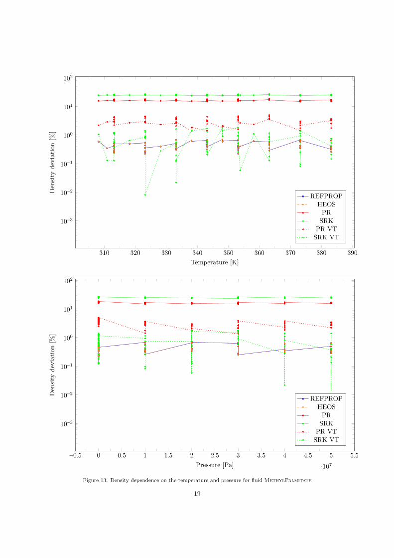
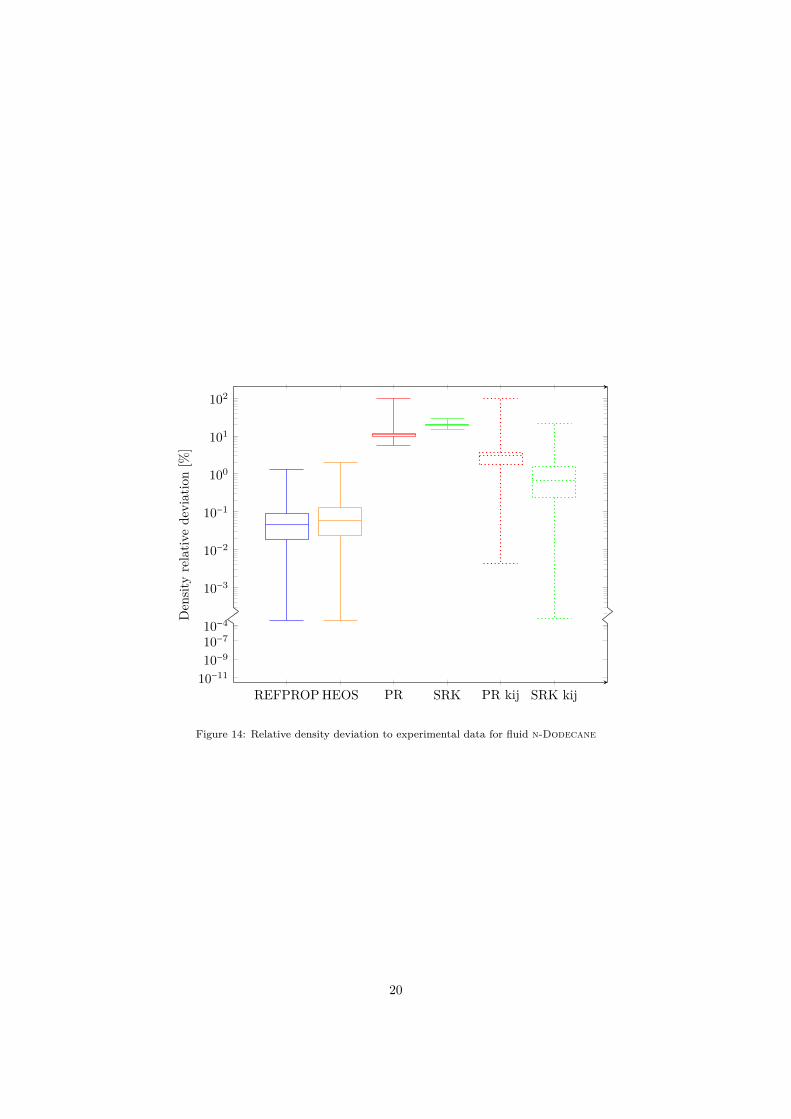
10minus4
10minus3
10minus2
10minus1
100
101
102
REFPROP HEOS PR SRK PR kij SRK kij10minus1110minus910minus7
Den
sity
rela
tive
devi
atio
n[
]
Figure 14 Relative density deviation to experimental data for fluid n-Dodecane
20
250 300 350 400 450 500 550 600 650
10minus3
10minus2
10minus1
100
101
102
Temperature [K]
Den
sity
devi
atio
n[
]
REFPROPHEOS
PRSRK
PR VTSRK VT
minus05 0 05 1 15 2 25 3 35 4 45 5 55 6 65 7 75
middot108
10minus3
10minus2
10minus1
100
101
102
Pressure [Pa]
Den
sity
devi
atio
n[
]
REFPROPHEOS
PRSRK
PR VTSRK VT
Figure 15 Density dependence on the temperature and pressure for fluid n-Dodecane
21
42 Binary mixturesAn other data set of experimental data has been collected by NIST for mixtures but only containing
vapour-liquid equilibrium (VLE) dataThese data consist of the molar fraction of each component and the temperature and pressure The
molar fraction at a given temperature and pressure are specified to be either liquid or gaseous which allowsto define the quality (0 or 1)
Two values where computed thanks to the state models the temperature from the pressure and thequality and the pressure from the temperature and quality The deviation between the computed valuesand the experimental data where then computed as following
ET =Tdata minus Tcalc
Tdata(32)
Ep =pdata minus pcalc
pdata(33)
The effect of the volume translation has not been evaluated here as no densityvolume data whereprovided
As these are mixtures there is the possibility to use an interaction parameter The one currentlyimplemented in CoolProp is the Van der Waals mixing rules with one parameter ki j For this work theinteraction parameter was fitted to minimize the deviation to experimental data with Brentrsquos method Theerror to minimise was expressed as follow
E =sum∣∣∣ET + 01Ep
∣∣∣ (34)
were ET and Ep are from equations 32 and 33The difference of results between pure temperature or pure pressure errors where not significant The
pressure term has been weighted by 01 as itrsquos magnitude was around 10 times bigger than the deviation interm of temperature
With the mixture the differences between RefProp and CoolProprsquos HEOS are a bit more marked as canbe seen in Figure 16 Depending on the fluid RefProp can be better than CoolProprsquos HEOS especiallywhen it comes to near critical data where the later tend to gives very wrong values (see Figure 18) but theFigure 19 is a good example where CoolProprsquos HEOS is far better
On the cubicrsquos side the results for the liquid-vapour equilibrium seems extremely good and comparablewith RefProp and CoolProprsquos HEOS It is interesting to notice that the volume translation problem occurringwith density and volume value do not seem to be a weight for these VLE data
A very important thing to notice with the mixture R1234YF-R134A is the influence of the molar fractionon the deviation (Figure 20) RefProp and the two cubics (without the binary interaction parameter ki j)have a deviation that considerable increases (around 10 times bigger) when mixing the two fluid comparedto the pure fluids with a maximum around equimolar composition This is the kind of behaviour that isexpected when using two sufficiently different fluids the way they interact together is different to the waythey interact with themselves
This effect is reduced with the interaction model and it appears that CoolProprsquos HEOS have a goodinteraction model for this mixture This is also corrected for the cubic by the ki j interaction parameterThis explains the better behaviour of CoolProprsquos HEOS and the cubics with interaction parameter for thisparticular mixture
Other mixtures like R134A-R32 are more similar and donrsquot benefit that much from a better mixing rule(Figure 17) This lead to more homogeneous deviations between the EOS
Again the variation of temperature and pressure on the relative deviation seems minimal except whenapproaching to the critical point
The temperature deviations are significantly smaller than the pressure deviations for all EOS
22
10minus4
10minus3
10minus2
10minus1
100
101
102
REFPROP HEOS PR SRK PR kij SRK kij10minus11
10minus9
10minus7Tem
pera
ture
rela
tive
devi
atio
n[
]
(a) Temperature deviation
10minus4
10minus3
10minus2
10minus1
100
101
102
REFPROP HEOS PR SRK PR kij SRK kij10minus11
10minus9
10minus7
Pres
sure
rela
tive
devi
atio
n[
]
(b) Pressure deviation
Figure 16 Relative deviation to experimental saturation data for mixtures based on R125 and R134A
23
0 01 02 03 04 05 06 07 08 09 110minus4
10minus3
10minus2
10minus1
100
Molar fraction of R134A [minus]
Tem
pera
ture
devi
atio
n[
]
REFPROPHEOS
PRSRK
PR ki jSRK ki j
0 01 02 03 04 05 06 07 08 09 110minus3
10minus2
10minus1
100
101
Molar fraction of R134A [minus]
Pres
sure
devi
atio
n[
]
REFPROPHEOS
PRSRK
PR ki jSRK ki j
Figure 17 Dependence on the molar fraction for the binary mixture R134A-R32
24
190 200 210 220 230 240 250 260 270 280 290 300 310 320 330 340 350 36010minus4
10minus3
10minus2
10minus1
100
Temperature [K]
Tem
pera
ture
devi
atio
n[
]
REFPROPHEOS
PRSRK
PR ki jSRK ki j
0 05 1 15 2 25 3 35 4
middot106
10minus3
10minus2
10minus1
100
101
Pressure [Pa]
Pres
sure
devi
atio
n[
]
REFPROPHEOS
PRSRK
PR ki jSRK ki j
Figure 18 Dependence on the temperature and pressure for the binary mixture R134A-R32
25
10minus4
10minus3
10minus2
10minus1
100
101
102
REFPROP HEOS PR SRK PR kij SRK kij10minus11
10minus9
10minus7Tem
pera
ture
rela
tive
devi
atio
n[
]
(a) Temperature deviation
10minus4
10minus3
10minus2
10minus1
100
101
102
REFPROP HEOS PR SRK PR kij SRK kij10minus11
10minus9
10minus7
Pres
sure
rela
tive
devi
atio
n[
]
(b) Pressure deviation
Figure 19 Relative deviation to experimental saturation data for mixtures based on R1234YF and R134A
26
0 01 02 03 04 05 06 07 08 09 110minus4
10minus3
10minus2
10minus1
100
Molar fraction of R1234YF [minus]
Tem
pera
ture
devi
atio
n[
]
REFPROPHEOS
PRSRK
PR ki jSRK ki j
0 01 02 03 04 05 06 07 08 09 110minus3
10minus2
10minus1
100
101
Molar fraction of R1234YF [minus]
Pres
sure
devi
atio
n[
]
REFPROPHEOS
PRSRK
PR ki jSRK ki j
Figure 20 Dependence on the molar fraction for the binary mixture R1234YF-R134A
27
270 275 280 285 290 295 300 305 310 315 320 325 330 335 34010minus4
10minus3
10minus2
10minus1
100
Temperature [K]
Tem
pera
ture
devi
atio
n[
]
REFPROPHEOS
PRSRK
PR ki jSRK ki j
02 03 04 05 06 07 08 09 1 11 12 13 14 15 16 17 18
middot106
10minus3
10minus2
10minus1
100
101
Pressure [Pa]
Pres
sure
devi
atio
n[
]
REFPROPHEOS
PRSRK
PR ki jSRK ki j
Figure 21 Dependence on the temperature and pressure for the binary mixture R1234YF-R134A
28
43 Ternary mixturesThe ternary mixtures are from the same data set as the binaries The binary interaction parameters ki j
where fitted with the binary mixture and reused hereThe results for the ternary mixtures are similar to the ones from the binaries
29
10minus4
10minus3
10minus2
10minus1
100
101
102
REFPROP HEOS PR SRK PR kij SRK kij10minus11
10minus9
10minus7Tem
pera
ture
rela
tive
devi
atio
n[
]
(a) Temperature deviation
10minus4
10minus3
10minus2
10minus1
100
101
102
REFPROP HEOS PR SRK PR kij SRK kij10minus11
10minus9
10minus7
Pres
sure
rela
tive
devi
atio
n[
]
(b) Pressure deviation
Figure 22 Relative deviation to experimental saturation data for mixtures based on R125 R32 and R134A
30
200 210 220 230 240 250 260 270 280 290 300 310 320 330 340 35010minus4
10minus3
10minus2
10minus1
100
Temperature [K]
Tem
pera
ture
devi
atio
n[
]
REFPROPHEOS
PRSRK
PR ki jSRK ki j
minus02 0 02 04 06 08 1 12 14 16 18 2 22 24 26 28 3 32 34 36 38
middot106
10minus3
10minus2
10minus1
100
101
Pressure [Pa]
Pres
sure
devi
atio
n[
]
REFPROPHEOS
PRSRK
PR ki jSRK ki j
Figure 23 Dependence on the temperature and pressure for the ternary mixture R125-R32-R134A
31
5 Acknowledgements
I would like to thank the professor Sylvain Quoilin for having given to me the opportunity to make thismaster thesis abroad This was a very interesting experience which allowed me to practice English and meetan other culture
I have a big thank to give to the DTU team who took care of me in Denmark the professor FredrikHaglind and the two post doctorates Maria E Mondejar Montagud and Jorrit Wronski It was a realpleasure to work with them
I also thanks Ian Bell our contact at NIST who manage to provide us with the database and withoutwho CoolProp would not exist
32
6 Conclusions
The simple cubic equations of state do not always gives satisfying results to compute density This canhowever be mostly corrected with a simple translation coefficient requiring a single measurement of saturatedliquid and more complex translation models could potentially give more accurate results
The cubic equations of states are very effective at modelling the liquid vapour equilibrium competingwith well recognise software
Depending on the interaction between the fluid constituting the mixtures all models benefit from binaryinteraction knowledge This is sometimes integrated in the software but would generally be an issue withnot yet well studied mixtures A simple coefficient (to be determined experimentally or approximated) canbe used to improve greatly the results of cubic equations when the interaction between the fluids is signif-icant An alternative would be to approximate the interaction with the UNIFAQ model as it is done withthe VTPR Determination of models to approximate the binary interaction parameters depending on thetype of fluid used would be an interesting subject for complementary study
More complex models can be used for the attractive parameter like the Mathias-Copeman and the TWUequations They both require 3 supplementary parameters and are already implemented in CoolProp Theirimpact could be interesting for a further study
The speed of the models are not compared in this work The comparison would be interesting butit is useful to notice CoolProp also provide a tabular interface which allows for extremely fast propertiescomputation when the tables have been generated (with a small loss of accuracy)
The cubic equations of states gives a wide range of possibilities from the simplest and fast model butslightly lacking accuracy to more complex and accurate models They provide a great tool for evaluation offluids when few data are available
33
Ahlers J Gmehling J 2001 Development of an universal group contribution equation of state Prediction of liquid densitiesfor pure compounds with a volume translated Peng-Robinson equation of state Fluid Phase Equilibria 191 (1-2) 177ndash188URL httpwwwsciencedirectcomsciencearticlepiiS0378381201006264pdfftmd5=86daea9e53bace87587e62b056b3007eamppid=1-s20-S0378381201006264-mainpdf
Bell I Jaumlger A 2016a Helmholtz energy transformation of common cubic equations of state for use with pure fluids andmixtures Journal of Research of the National Institute of Standards and Technology 121 (July) 238ndash263URL httpswwwresearchgatenetpublication304186500_Helmholtz_Energy_Transformations_of_Common_Cubic_Equations_of_State_for_Use_with_Pure_Fluids_and_Mixtures
Bell I H Jaumlger A 2016b Intermediate Terms 1ndash14Bell I H Jaumlger A 2016c Supplementary Information to accompany Helmholtz energy transformations of common cubic
equations of state for use with pure fluids and mixtures No 5Chen W-Y Liu J 2007 Mathcad Modules for Supercritical Fluid Extraction based on Mixing Rules Appendix A - Mixing
Rules (662) 1ndash10URL httphomeolemissedu~cmchengsExtractionAppendixA_MixingRulesdoc
CoolProp 2016 Cubic Equations of StateURL httpwwwcoolproporgcoolpropCubicshtml
Fauacutendez C a Valderrama J O 2009 Low pressure vaporndashliquid equilibrium in ethanol+congener mixtures using theWongndashSandler mixing rule Thermochimica Acta 490 (1-2) 37ndash42URL httpwwwsciencedirectcomsciencearticlepiiS0040603109000999pdfftmd5=65533f85d53569eeebae29e565402cc4amppid=1-s20-S0040603109000999-mainpdf
Frey K Augustine C Ciccolini R P Paap S Modell M Tester J 2007 Volume translation in equations of state as ameans of accurate property estimation Fluid Phase Equilibria 260 (2) 316ndash325URL httpwwwsciencedirectcomsciencearticlepiiS0378381207004591pdfftmd5=c750d4ea93f662a13b87183c76a8654eamppid=1-s20-S0378381207004591-mainpdf
Ji W-R Lempe D 1997 Density improvement of the SRK equation of state Fluid Phase Equilibria 130 (1-2) 49ndash63URL httpwwwsciencedirectcomsciencearticlepiiS0378381296031901
Lemmon E W Huber M L McLinden M O 2013 Reference Fluid Thermodynamic and Transport Properties-REFPROPversion 91URL httpwwwnistgovsrduploadREFPROP9PDF
Loacutepez J A Cardona C A 2006 Phase equilibrium calculations for carbon dioxide+n-alkanes binary mixtures with theWongndashSandler mixing rules Fluid Phase Equilibria 239 (2) 206ndash212URL httpwwwsciencedirectcomsciencearticlepiiS0378381205004565
Martin J J 1967 Equations of StatemdashApplied Thermodynamics Symposium Industrial amp Engineering Chemistry 59 (12)34ndash52URL httpdxdoiorg101021ie50696a008$delimiter026E30F$nhttppubsacsorgdoipdf101021ie50696a008
Martin J J 1979 Cubic Equations of State-Which Industrial amp Engineering Chemistry Fundamentals 18 (2) 81ndash97URL httpdxdoiorg101021i160070a001
Meng L Duan Y Y Wang X D 2007 Binary interaction parameter kij for calculating the second cross-virial coefficientsof mixtures Fluid Phase Equilibria 260 (2) 354ndash358URL httpwwwsciencedirectcomsciencearticlepiiS0378381207004323pdfftmd5=e3b19d08e08099003d28392a4450f768amppid=1-s20-S0378381207004323-mainpdf
Peng D-Y Robinson D B 1976 A New Two-Constant Equation of State Industrial amp Engineering Chemistry Fundamentals15 (1) 59ndash64URL httppubsacsorgdoiabs101021i160057a011
Schmid B Gmehling J 2012 Revised parameters and typical results of the VTPR group contribution equation of stateFluid Phase Equilibria 317 110ndash126URL httpdxdoiorg101016jfluid201201006
Schmid B Schedemann A Gmehling J 2014 Extension of the VTPR group contribution equation of state Groupinteraction parameters for additional 192 group combinations and typical results Industrial and Engineering ChemistryResearch 53 (8) 3393ndash3405
Soave G 1972 Equilibrium constants from a modified Redlich-Kwong equation of state Chemical Engineering Science 27 (6)1197ndash1203URL httpacels-cdncom00092509728009641-s20-0009250972800964-mainpdf_tid=cd3fc6c8-1dbd-11e6-a8de-00000aacb35dampacdnat=1463661351_8f1dbe034b52854e2d97cd6d80b7b56b
Valderrama J O 2003 The State of the Cubic Equations of State Industrial amp Engineering Chemistry Research 42 (8)1603ndash1618URL httppubsacsorgdoiabs101021ie020447b
Valderrama J O Marambio L E Silva A a 2002 Mixing rules in cubic equations of state applied to refrigerant mixturesJournal of Phase Equilibria 23 (6) 495ndash501URL httpdownloadspringercomstaticpdf558art3A1013612F105497102770331181pdforiginUrl=httplinkspringercomarticle101361105497102770331181amptoken2=exp=1463652668~acl=staticpdf558art253A101361252F105497102770
Wong D S H Sandler S I 1992 A Theoretically Correct Mixing Rule for Cubic Equations of State 38 (5)URL httponlinelibrarywileycomdoi101002aic690380505epdf
34
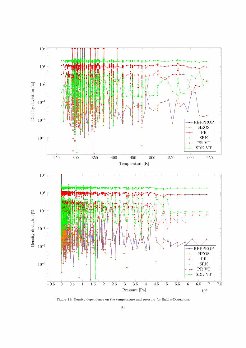
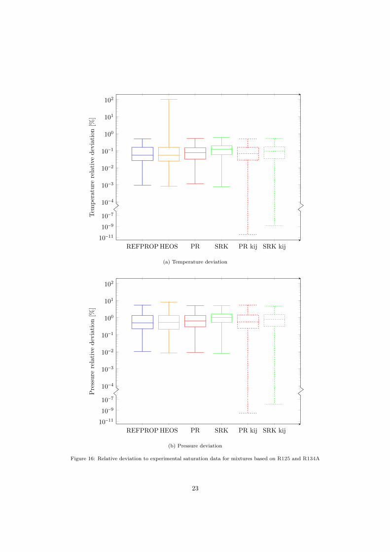
10minus4
10minus3
10minus2
10minus1
100
101
102
REFPROP HEOS PR SRK PR kij SRK kij10minus11
10minus9
10minus7Tem
pera
ture
rela
tive
devi
atio
n[
]
(a) Temperature deviation
10minus4
10minus3
10minus2
10minus1
100
101
102
REFPROP HEOS PR SRK PR kij SRK kij10minus11
10minus9
10minus7
Pres
sure
rela
tive
devi
atio
n[
]
(b) Pressure deviation
Figure 16 Relative deviation to experimental saturation data for mixtures based on R125 and R134A
23
0 01 02 03 04 05 06 07 08 09 110minus4
10minus3
10minus2
10minus1
100
Molar fraction of R134A [minus]
Tem
pera
ture
devi
atio
n[
]
REFPROPHEOS
PRSRK
PR ki jSRK ki j
0 01 02 03 04 05 06 07 08 09 110minus3
10minus2
10minus1
100
101
Molar fraction of R134A [minus]
Pres
sure
devi
atio
n[
]
REFPROPHEOS
PRSRK
PR ki jSRK ki j
Figure 17 Dependence on the molar fraction for the binary mixture R134A-R32
24
190 200 210 220 230 240 250 260 270 280 290 300 310 320 330 340 350 36010minus4
10minus3
10minus2
10minus1
100
Temperature [K]
Tem
pera
ture
devi
atio
n[
]
REFPROPHEOS
PRSRK
PR ki jSRK ki j
0 05 1 15 2 25 3 35 4
middot106
10minus3
10minus2
10minus1
100
101
Pressure [Pa]
Pres
sure
devi
atio
n[
]
REFPROPHEOS
PRSRK
PR ki jSRK ki j
Figure 18 Dependence on the temperature and pressure for the binary mixture R134A-R32
25
10minus4
10minus3
10minus2
10minus1
100
101
102
REFPROP HEOS PR SRK PR kij SRK kij10minus11
10minus9
10minus7Tem
pera
ture
rela
tive
devi
atio
n[
]
(a) Temperature deviation
10minus4
10minus3
10minus2
10minus1
100
101
102
REFPROP HEOS PR SRK PR kij SRK kij10minus11
10minus9
10minus7
Pres
sure
rela
tive
devi
atio
n[
]
(b) Pressure deviation
Figure 19 Relative deviation to experimental saturation data for mixtures based on R1234YF and R134A
26
0 01 02 03 04 05 06 07 08 09 110minus4
10minus3
10minus2
10minus1
100
Molar fraction of R1234YF [minus]
Tem
pera
ture
devi
atio
n[
]
REFPROPHEOS
PRSRK
PR ki jSRK ki j
0 01 02 03 04 05 06 07 08 09 110minus3
10minus2
10minus1
100
101
Molar fraction of R1234YF [minus]
Pres
sure
devi
atio
n[
]
REFPROPHEOS
PRSRK
PR ki jSRK ki j
Figure 20 Dependence on the molar fraction for the binary mixture R1234YF-R134A
27
270 275 280 285 290 295 300 305 310 315 320 325 330 335 34010minus4
10minus3
10minus2
10minus1
100
Temperature [K]
Tem
pera
ture
devi
atio
n[
]
REFPROPHEOS
PRSRK
PR ki jSRK ki j
02 03 04 05 06 07 08 09 1 11 12 13 14 15 16 17 18
middot106
10minus3
10minus2
10minus1
100
101
Pressure [Pa]
Pres
sure
devi
atio
n[
]
REFPROPHEOS
PRSRK
PR ki jSRK ki j
Figure 21 Dependence on the temperature and pressure for the binary mixture R1234YF-R134A
28
43 Ternary mixturesThe ternary mixtures are from the same data set as the binaries The binary interaction parameters ki j
where fitted with the binary mixture and reused hereThe results for the ternary mixtures are similar to the ones from the binaries
29
10minus4
10minus3
10minus2
10minus1
100
101
102
REFPROP HEOS PR SRK PR kij SRK kij10minus11
10minus9
10minus7Tem
pera
ture
rela
tive
devi
atio
n[
]
(a) Temperature deviation
10minus4
10minus3
10minus2
10minus1
100
101
102
REFPROP HEOS PR SRK PR kij SRK kij10minus11
10minus9
10minus7
Pres
sure
rela
tive
devi
atio
n[
]
(b) Pressure deviation
Figure 22 Relative deviation to experimental saturation data for mixtures based on R125 R32 and R134A
30
200 210 220 230 240 250 260 270 280 290 300 310 320 330 340 35010minus4
10minus3
10minus2
10minus1
100
Temperature [K]
Tem
pera
ture
devi
atio
n[
]
REFPROPHEOS
PRSRK
PR ki jSRK ki j
minus02 0 02 04 06 08 1 12 14 16 18 2 22 24 26 28 3 32 34 36 38
middot106
10minus3
10minus2
10minus1
100
101
Pressure [Pa]
Pres
sure
devi
atio
n[
]
REFPROPHEOS
PRSRK
PR ki jSRK ki j
Figure 23 Dependence on the temperature and pressure for the ternary mixture R125-R32-R134A
31
5 Acknowledgements
I would like to thank the professor Sylvain Quoilin for having given to me the opportunity to make thismaster thesis abroad This was a very interesting experience which allowed me to practice English and meetan other culture
I have a big thank to give to the DTU team who took care of me in Denmark the professor FredrikHaglind and the two post doctorates Maria E Mondejar Montagud and Jorrit Wronski It was a realpleasure to work with them
I also thanks Ian Bell our contact at NIST who manage to provide us with the database and withoutwho CoolProp would not exist
32
6 Conclusions
The simple cubic equations of state do not always gives satisfying results to compute density This canhowever be mostly corrected with a simple translation coefficient requiring a single measurement of saturatedliquid and more complex translation models could potentially give more accurate results
The cubic equations of states are very effective at modelling the liquid vapour equilibrium competingwith well recognise software
Depending on the interaction between the fluid constituting the mixtures all models benefit from binaryinteraction knowledge This is sometimes integrated in the software but would generally be an issue withnot yet well studied mixtures A simple coefficient (to be determined experimentally or approximated) canbe used to improve greatly the results of cubic equations when the interaction between the fluids is signif-icant An alternative would be to approximate the interaction with the UNIFAQ model as it is done withthe VTPR Determination of models to approximate the binary interaction parameters depending on thetype of fluid used would be an interesting subject for complementary study
More complex models can be used for the attractive parameter like the Mathias-Copeman and the TWUequations They both require 3 supplementary parameters and are already implemented in CoolProp Theirimpact could be interesting for a further study
The speed of the models are not compared in this work The comparison would be interesting butit is useful to notice CoolProp also provide a tabular interface which allows for extremely fast propertiescomputation when the tables have been generated (with a small loss of accuracy)
The cubic equations of states gives a wide range of possibilities from the simplest and fast model butslightly lacking accuracy to more complex and accurate models They provide a great tool for evaluation offluids when few data are available
33
Ahlers J Gmehling J 2001 Development of an universal group contribution equation of state Prediction of liquid densitiesfor pure compounds with a volume translated Peng-Robinson equation of state Fluid Phase Equilibria 191 (1-2) 177ndash188URL httpwwwsciencedirectcomsciencearticlepiiS0378381201006264pdfftmd5=86daea9e53bace87587e62b056b3007eamppid=1-s20-S0378381201006264-mainpdf
Bell I Jaumlger A 2016a Helmholtz energy transformation of common cubic equations of state for use with pure fluids andmixtures Journal of Research of the National Institute of Standards and Technology 121 (July) 238ndash263URL httpswwwresearchgatenetpublication304186500_Helmholtz_Energy_Transformations_of_Common_Cubic_Equations_of_State_for_Use_with_Pure_Fluids_and_Mixtures
Bell I H Jaumlger A 2016b Intermediate Terms 1ndash14Bell I H Jaumlger A 2016c Supplementary Information to accompany Helmholtz energy transformations of common cubic
equations of state for use with pure fluids and mixtures No 5Chen W-Y Liu J 2007 Mathcad Modules for Supercritical Fluid Extraction based on Mixing Rules Appendix A - Mixing
Rules (662) 1ndash10URL httphomeolemissedu~cmchengsExtractionAppendixA_MixingRulesdoc
CoolProp 2016 Cubic Equations of StateURL httpwwwcoolproporgcoolpropCubicshtml
Fauacutendez C a Valderrama J O 2009 Low pressure vaporndashliquid equilibrium in ethanol+congener mixtures using theWongndashSandler mixing rule Thermochimica Acta 490 (1-2) 37ndash42URL httpwwwsciencedirectcomsciencearticlepiiS0040603109000999pdfftmd5=65533f85d53569eeebae29e565402cc4amppid=1-s20-S0040603109000999-mainpdf
Frey K Augustine C Ciccolini R P Paap S Modell M Tester J 2007 Volume translation in equations of state as ameans of accurate property estimation Fluid Phase Equilibria 260 (2) 316ndash325URL httpwwwsciencedirectcomsciencearticlepiiS0378381207004591pdfftmd5=c750d4ea93f662a13b87183c76a8654eamppid=1-s20-S0378381207004591-mainpdf
Ji W-R Lempe D 1997 Density improvement of the SRK equation of state Fluid Phase Equilibria 130 (1-2) 49ndash63URL httpwwwsciencedirectcomsciencearticlepiiS0378381296031901
Lemmon E W Huber M L McLinden M O 2013 Reference Fluid Thermodynamic and Transport Properties-REFPROPversion 91URL httpwwwnistgovsrduploadREFPROP9PDF
Loacutepez J A Cardona C A 2006 Phase equilibrium calculations for carbon dioxide+n-alkanes binary mixtures with theWongndashSandler mixing rules Fluid Phase Equilibria 239 (2) 206ndash212URL httpwwwsciencedirectcomsciencearticlepiiS0378381205004565
Martin J J 1967 Equations of StatemdashApplied Thermodynamics Symposium Industrial amp Engineering Chemistry 59 (12)34ndash52URL httpdxdoiorg101021ie50696a008$delimiter026E30F$nhttppubsacsorgdoipdf101021ie50696a008
Martin J J 1979 Cubic Equations of State-Which Industrial amp Engineering Chemistry Fundamentals 18 (2) 81ndash97URL httpdxdoiorg101021i160070a001
Meng L Duan Y Y Wang X D 2007 Binary interaction parameter kij for calculating the second cross-virial coefficientsof mixtures Fluid Phase Equilibria 260 (2) 354ndash358URL httpwwwsciencedirectcomsciencearticlepiiS0378381207004323pdfftmd5=e3b19d08e08099003d28392a4450f768amppid=1-s20-S0378381207004323-mainpdf
Peng D-Y Robinson D B 1976 A New Two-Constant Equation of State Industrial amp Engineering Chemistry Fundamentals15 (1) 59ndash64URL httppubsacsorgdoiabs101021i160057a011
Schmid B Gmehling J 2012 Revised parameters and typical results of the VTPR group contribution equation of stateFluid Phase Equilibria 317 110ndash126URL httpdxdoiorg101016jfluid201201006
Schmid B Schedemann A Gmehling J 2014 Extension of the VTPR group contribution equation of state Groupinteraction parameters for additional 192 group combinations and typical results Industrial and Engineering ChemistryResearch 53 (8) 3393ndash3405
Soave G 1972 Equilibrium constants from a modified Redlich-Kwong equation of state Chemical Engineering Science 27 (6)1197ndash1203URL httpacels-cdncom00092509728009641-s20-0009250972800964-mainpdf_tid=cd3fc6c8-1dbd-11e6-a8de-00000aacb35dampacdnat=1463661351_8f1dbe034b52854e2d97cd6d80b7b56b
Valderrama J O 2003 The State of the Cubic Equations of State Industrial amp Engineering Chemistry Research 42 (8)1603ndash1618URL httppubsacsorgdoiabs101021ie020447b
Valderrama J O Marambio L E Silva A a 2002 Mixing rules in cubic equations of state applied to refrigerant mixturesJournal of Phase Equilibria 23 (6) 495ndash501URL httpdownloadspringercomstaticpdf558art3A1013612F105497102770331181pdforiginUrl=httplinkspringercomarticle101361105497102770331181amptoken2=exp=1463652668~acl=staticpdf558art253A101361252F105497102770
Wong D S H Sandler S I 1992 A Theoretically Correct Mixing Rule for Cubic Equations of State 38 (5)URL httponlinelibrarywileycomdoi101002aic690380505epdf
34
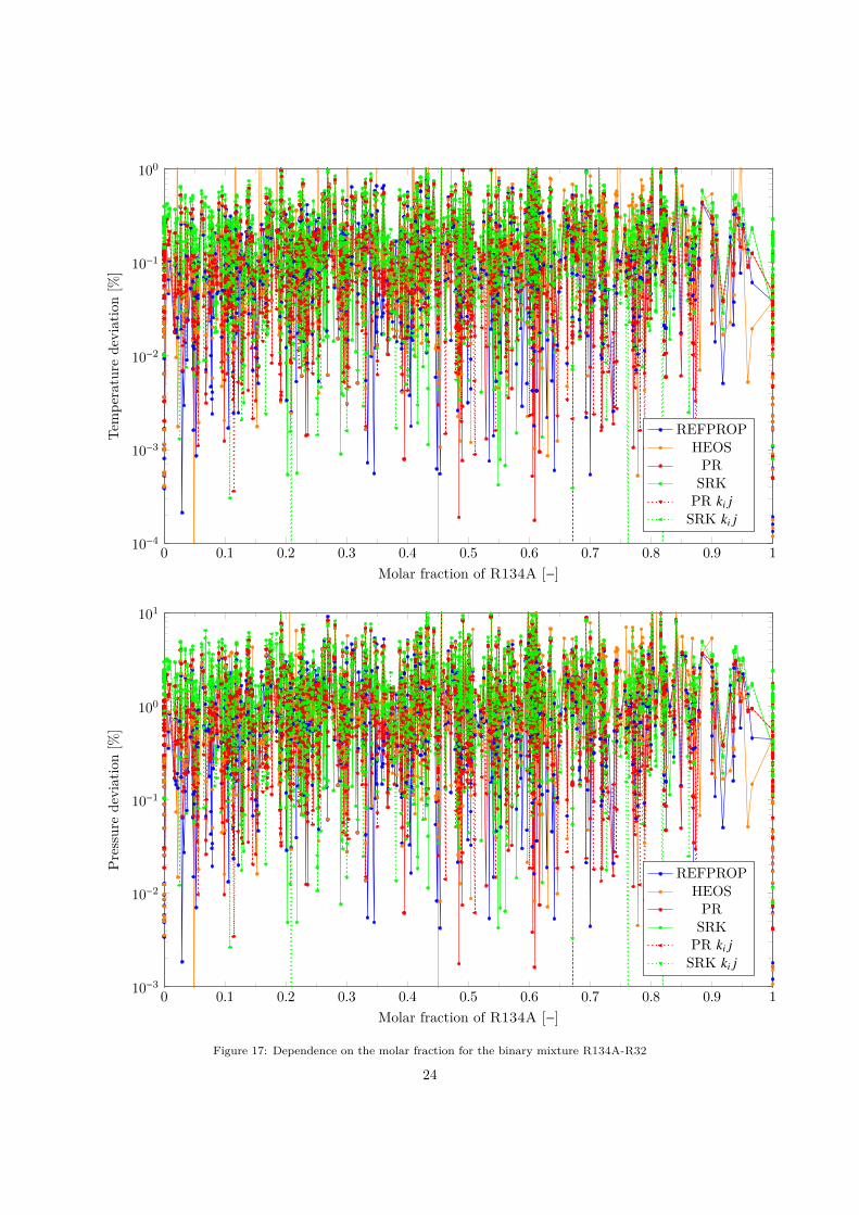
0 01 02 03 04 05 06 07 08 09 110minus4
10minus3
10minus2
10minus1
100
Molar fraction of R134A [minus]
Tem
pera
ture
devi
atio
n[
]
REFPROPHEOS
PRSRK
PR ki jSRK ki j
0 01 02 03 04 05 06 07 08 09 110minus3
10minus2
10minus1
100
101
Molar fraction of R134A [minus]
Pres
sure
devi
atio
n[
]
REFPROPHEOS
PRSRK
PR ki jSRK ki j
Figure 17 Dependence on the molar fraction for the binary mixture R134A-R32
24
190 200 210 220 230 240 250 260 270 280 290 300 310 320 330 340 350 36010minus4
10minus3
10minus2
10minus1
100
Temperature [K]
Tem
pera
ture
devi
atio
n[
]
REFPROPHEOS
PRSRK
PR ki jSRK ki j
0 05 1 15 2 25 3 35 4
middot106
10minus3
10minus2
10minus1
100
101
Pressure [Pa]
Pres
sure
devi
atio
n[
]
REFPROPHEOS
PRSRK
PR ki jSRK ki j
Figure 18 Dependence on the temperature and pressure for the binary mixture R134A-R32
25
10minus4
10minus3
10minus2
10minus1
100
101
102
REFPROP HEOS PR SRK PR kij SRK kij10minus11
10minus9
10minus7Tem
pera
ture
rela
tive
devi
atio
n[
]
(a) Temperature deviation
10minus4
10minus3
10minus2
10minus1
100
101
102
REFPROP HEOS PR SRK PR kij SRK kij10minus11
10minus9
10minus7
Pres
sure
rela
tive
devi
atio
n[
]
(b) Pressure deviation
Figure 19 Relative deviation to experimental saturation data for mixtures based on R1234YF and R134A
26
0 01 02 03 04 05 06 07 08 09 110minus4
10minus3
10minus2
10minus1
100
Molar fraction of R1234YF [minus]
Tem
pera
ture
devi
atio
n[
]
REFPROPHEOS
PRSRK
PR ki jSRK ki j
0 01 02 03 04 05 06 07 08 09 110minus3
10minus2
10minus1
100
101
Molar fraction of R1234YF [minus]
Pres
sure
devi
atio
n[
]
REFPROPHEOS
PRSRK
PR ki jSRK ki j
Figure 20 Dependence on the molar fraction for the binary mixture R1234YF-R134A
27
270 275 280 285 290 295 300 305 310 315 320 325 330 335 34010minus4
10minus3
10minus2
10minus1
100
Temperature [K]
Tem
pera
ture
devi
atio
n[
]
REFPROPHEOS
PRSRK
PR ki jSRK ki j
02 03 04 05 06 07 08 09 1 11 12 13 14 15 16 17 18
middot106
10minus3
10minus2
10minus1
100
101
Pressure [Pa]
Pres
sure
devi
atio
n[
]
REFPROPHEOS
PRSRK
PR ki jSRK ki j
Figure 21 Dependence on the temperature and pressure for the binary mixture R1234YF-R134A
28
43 Ternary mixturesThe ternary mixtures are from the same data set as the binaries The binary interaction parameters ki j
where fitted with the binary mixture and reused hereThe results for the ternary mixtures are similar to the ones from the binaries
29
10minus4
10minus3
10minus2
10minus1
100
101
102
REFPROP HEOS PR SRK PR kij SRK kij10minus11
10minus9
10minus7Tem
pera
ture
rela
tive
devi
atio
n[
]
(a) Temperature deviation
10minus4
10minus3
10minus2
10minus1
100
101
102
REFPROP HEOS PR SRK PR kij SRK kij10minus11
10minus9
10minus7
Pres
sure
rela
tive
devi
atio
n[
]
(b) Pressure deviation
Figure 22 Relative deviation to experimental saturation data for mixtures based on R125 R32 and R134A
30
200 210 220 230 240 250 260 270 280 290 300 310 320 330 340 35010minus4
10minus3
10minus2
10minus1
100
Temperature [K]
Tem
pera
ture
devi
atio
n[
]
REFPROPHEOS
PRSRK
PR ki jSRK ki j
minus02 0 02 04 06 08 1 12 14 16 18 2 22 24 26 28 3 32 34 36 38
middot106
10minus3
10minus2
10minus1
100
101
Pressure [Pa]
Pres
sure
devi
atio
n[
]
REFPROPHEOS
PRSRK
PR ki jSRK ki j
Figure 23 Dependence on the temperature and pressure for the ternary mixture R125-R32-R134A
31
5 Acknowledgements
I would like to thank the professor Sylvain Quoilin for having given to me the opportunity to make thismaster thesis abroad This was a very interesting experience which allowed me to practice English and meetan other culture
I have a big thank to give to the DTU team who took care of me in Denmark the professor FredrikHaglind and the two post doctorates Maria E Mondejar Montagud and Jorrit Wronski It was a realpleasure to work with them
I also thanks Ian Bell our contact at NIST who manage to provide us with the database and withoutwho CoolProp would not exist
32
6 Conclusions
The simple cubic equations of state do not always gives satisfying results to compute density This canhowever be mostly corrected with a simple translation coefficient requiring a single measurement of saturatedliquid and more complex translation models could potentially give more accurate results
The cubic equations of states are very effective at modelling the liquid vapour equilibrium competingwith well recognise software
Depending on the interaction between the fluid constituting the mixtures all models benefit from binaryinteraction knowledge This is sometimes integrated in the software but would generally be an issue withnot yet well studied mixtures A simple coefficient (to be determined experimentally or approximated) canbe used to improve greatly the results of cubic equations when the interaction between the fluids is signif-icant An alternative would be to approximate the interaction with the UNIFAQ model as it is done withthe VTPR Determination of models to approximate the binary interaction parameters depending on thetype of fluid used would be an interesting subject for complementary study
More complex models can be used for the attractive parameter like the Mathias-Copeman and the TWUequations They both require 3 supplementary parameters and are already implemented in CoolProp Theirimpact could be interesting for a further study
The speed of the models are not compared in this work The comparison would be interesting butit is useful to notice CoolProp also provide a tabular interface which allows for extremely fast propertiescomputation when the tables have been generated (with a small loss of accuracy)
The cubic equations of states gives a wide range of possibilities from the simplest and fast model butslightly lacking accuracy to more complex and accurate models They provide a great tool for evaluation offluids when few data are available
33
Ahlers J Gmehling J 2001 Development of an universal group contribution equation of state Prediction of liquid densitiesfor pure compounds with a volume translated Peng-Robinson equation of state Fluid Phase Equilibria 191 (1-2) 177ndash188URL httpwwwsciencedirectcomsciencearticlepiiS0378381201006264pdfftmd5=86daea9e53bace87587e62b056b3007eamppid=1-s20-S0378381201006264-mainpdf
Bell I Jaumlger A 2016a Helmholtz energy transformation of common cubic equations of state for use with pure fluids andmixtures Journal of Research of the National Institute of Standards and Technology 121 (July) 238ndash263URL httpswwwresearchgatenetpublication304186500_Helmholtz_Energy_Transformations_of_Common_Cubic_Equations_of_State_for_Use_with_Pure_Fluids_and_Mixtures
Bell I H Jaumlger A 2016b Intermediate Terms 1ndash14Bell I H Jaumlger A 2016c Supplementary Information to accompany Helmholtz energy transformations of common cubic
equations of state for use with pure fluids and mixtures No 5Chen W-Y Liu J 2007 Mathcad Modules for Supercritical Fluid Extraction based on Mixing Rules Appendix A - Mixing
Rules (662) 1ndash10URL httphomeolemissedu~cmchengsExtractionAppendixA_MixingRulesdoc
CoolProp 2016 Cubic Equations of StateURL httpwwwcoolproporgcoolpropCubicshtml
Fauacutendez C a Valderrama J O 2009 Low pressure vaporndashliquid equilibrium in ethanol+congener mixtures using theWongndashSandler mixing rule Thermochimica Acta 490 (1-2) 37ndash42URL httpwwwsciencedirectcomsciencearticlepiiS0040603109000999pdfftmd5=65533f85d53569eeebae29e565402cc4amppid=1-s20-S0040603109000999-mainpdf
Frey K Augustine C Ciccolini R P Paap S Modell M Tester J 2007 Volume translation in equations of state as ameans of accurate property estimation Fluid Phase Equilibria 260 (2) 316ndash325URL httpwwwsciencedirectcomsciencearticlepiiS0378381207004591pdfftmd5=c750d4ea93f662a13b87183c76a8654eamppid=1-s20-S0378381207004591-mainpdf
Ji W-R Lempe D 1997 Density improvement of the SRK equation of state Fluid Phase Equilibria 130 (1-2) 49ndash63URL httpwwwsciencedirectcomsciencearticlepiiS0378381296031901
Lemmon E W Huber M L McLinden M O 2013 Reference Fluid Thermodynamic and Transport Properties-REFPROPversion 91URL httpwwwnistgovsrduploadREFPROP9PDF
Loacutepez J A Cardona C A 2006 Phase equilibrium calculations for carbon dioxide+n-alkanes binary mixtures with theWongndashSandler mixing rules Fluid Phase Equilibria 239 (2) 206ndash212URL httpwwwsciencedirectcomsciencearticlepiiS0378381205004565
Martin J J 1967 Equations of StatemdashApplied Thermodynamics Symposium Industrial amp Engineering Chemistry 59 (12)34ndash52URL httpdxdoiorg101021ie50696a008$delimiter026E30F$nhttppubsacsorgdoipdf101021ie50696a008
Martin J J 1979 Cubic Equations of State-Which Industrial amp Engineering Chemistry Fundamentals 18 (2) 81ndash97URL httpdxdoiorg101021i160070a001
Meng L Duan Y Y Wang X D 2007 Binary interaction parameter kij for calculating the second cross-virial coefficientsof mixtures Fluid Phase Equilibria 260 (2) 354ndash358URL httpwwwsciencedirectcomsciencearticlepiiS0378381207004323pdfftmd5=e3b19d08e08099003d28392a4450f768amppid=1-s20-S0378381207004323-mainpdf
Peng D-Y Robinson D B 1976 A New Two-Constant Equation of State Industrial amp Engineering Chemistry Fundamentals15 (1) 59ndash64URL httppubsacsorgdoiabs101021i160057a011
Schmid B Gmehling J 2012 Revised parameters and typical results of the VTPR group contribution equation of stateFluid Phase Equilibria 317 110ndash126URL httpdxdoiorg101016jfluid201201006
Schmid B Schedemann A Gmehling J 2014 Extension of the VTPR group contribution equation of state Groupinteraction parameters for additional 192 group combinations and typical results Industrial and Engineering ChemistryResearch 53 (8) 3393ndash3405
Soave G 1972 Equilibrium constants from a modified Redlich-Kwong equation of state Chemical Engineering Science 27 (6)1197ndash1203URL httpacels-cdncom00092509728009641-s20-0009250972800964-mainpdf_tid=cd3fc6c8-1dbd-11e6-a8de-00000aacb35dampacdnat=1463661351_8f1dbe034b52854e2d97cd6d80b7b56b
Valderrama J O 2003 The State of the Cubic Equations of State Industrial amp Engineering Chemistry Research 42 (8)1603ndash1618URL httppubsacsorgdoiabs101021ie020447b
Valderrama J O Marambio L E Silva A a 2002 Mixing rules in cubic equations of state applied to refrigerant mixturesJournal of Phase Equilibria 23 (6) 495ndash501URL httpdownloadspringercomstaticpdf558art3A1013612F105497102770331181pdforiginUrl=httplinkspringercomarticle101361105497102770331181amptoken2=exp=1463652668~acl=staticpdf558art253A101361252F105497102770
Wong D S H Sandler S I 1992 A Theoretically Correct Mixing Rule for Cubic Equations of State 38 (5)URL httponlinelibrarywileycomdoi101002aic690380505epdf
34
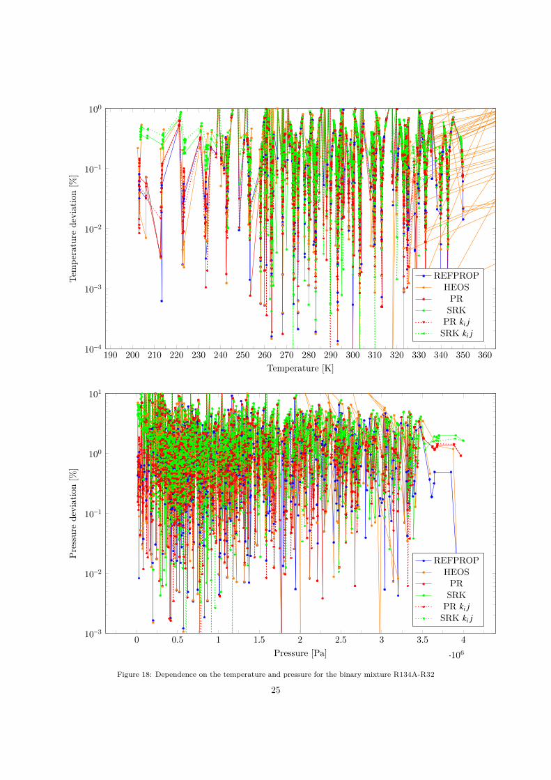
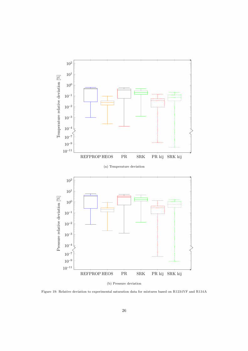
10minus4
10minus3
10minus2
10minus1
100
101
102
REFPROP HEOS PR SRK PR kij SRK kij10minus11
10minus9
10minus7Tem
pera
ture
rela
tive
devi
atio
n[
]
(a) Temperature deviation
10minus4
10minus3
10minus2
10minus1
100
101
102
REFPROP HEOS PR SRK PR kij SRK kij10minus11
10minus9
10minus7
Pres
sure
rela
tive
devi
atio
n[
]
(b) Pressure deviation
Figure 19 Relative deviation to experimental saturation data for mixtures based on R1234YF and R134A
26
0 01 02 03 04 05 06 07 08 09 110minus4
10minus3
10minus2
10minus1
100
Molar fraction of R1234YF [minus]
Tem
pera
ture
devi
atio
n[
]
REFPROPHEOS
PRSRK
PR ki jSRK ki j
0 01 02 03 04 05 06 07 08 09 110minus3
10minus2
10minus1
100
101
Molar fraction of R1234YF [minus]
Pres
sure
devi
atio
n[
]
REFPROPHEOS
PRSRK
PR ki jSRK ki j
Figure 20 Dependence on the molar fraction for the binary mixture R1234YF-R134A
27
270 275 280 285 290 295 300 305 310 315 320 325 330 335 34010minus4
10minus3
10minus2
10minus1
100
Temperature [K]
Tem
pera
ture
devi
atio
n[
]
REFPROPHEOS
PRSRK
PR ki jSRK ki j
02 03 04 05 06 07 08 09 1 11 12 13 14 15 16 17 18
middot106
10minus3
10minus2
10minus1
100
101
Pressure [Pa]
Pres
sure
devi
atio
n[
]
REFPROPHEOS
PRSRK
PR ki jSRK ki j
Figure 21 Dependence on the temperature and pressure for the binary mixture R1234YF-R134A
28
43 Ternary mixturesThe ternary mixtures are from the same data set as the binaries The binary interaction parameters ki j
where fitted with the binary mixture and reused hereThe results for the ternary mixtures are similar to the ones from the binaries
29
10minus4
10minus3
10minus2
10minus1
100
101
102
REFPROP HEOS PR SRK PR kij SRK kij10minus11
10minus9
10minus7Tem
pera
ture
rela
tive
devi
atio
n[
]
(a) Temperature deviation
10minus4
10minus3
10minus2
10minus1
100
101
102
REFPROP HEOS PR SRK PR kij SRK kij10minus11
10minus9
10minus7
Pres
sure
rela
tive
devi
atio
n[
]
(b) Pressure deviation
Figure 22 Relative deviation to experimental saturation data for mixtures based on R125 R32 and R134A
30
200 210 220 230 240 250 260 270 280 290 300 310 320 330 340 35010minus4
10minus3
10minus2
10minus1
100
Temperature [K]
Tem
pera
ture
devi
atio
n[
]
REFPROPHEOS
PRSRK
PR ki jSRK ki j
minus02 0 02 04 06 08 1 12 14 16 18 2 22 24 26 28 3 32 34 36 38
middot106
10minus3
10minus2
10minus1
100
101
Pressure [Pa]
Pres
sure
devi
atio
n[
]
REFPROPHEOS
PRSRK
PR ki jSRK ki j
Figure 23 Dependence on the temperature and pressure for the ternary mixture R125-R32-R134A
31
5 Acknowledgements
I would like to thank the professor Sylvain Quoilin for having given to me the opportunity to make thismaster thesis abroad This was a very interesting experience which allowed me to practice English and meetan other culture
I have a big thank to give to the DTU team who took care of me in Denmark the professor FredrikHaglind and the two post doctorates Maria E Mondejar Montagud and Jorrit Wronski It was a realpleasure to work with them
I also thanks Ian Bell our contact at NIST who manage to provide us with the database and withoutwho CoolProp would not exist
32
6 Conclusions
The simple cubic equations of state do not always gives satisfying results to compute density This canhowever be mostly corrected with a simple translation coefficient requiring a single measurement of saturatedliquid and more complex translation models could potentially give more accurate results
The cubic equations of states are very effective at modelling the liquid vapour equilibrium competingwith well recognise software
Depending on the interaction between the fluid constituting the mixtures all models benefit from binaryinteraction knowledge This is sometimes integrated in the software but would generally be an issue withnot yet well studied mixtures A simple coefficient (to be determined experimentally or approximated) canbe used to improve greatly the results of cubic equations when the interaction between the fluids is signif-icant An alternative would be to approximate the interaction with the UNIFAQ model as it is done withthe VTPR Determination of models to approximate the binary interaction parameters depending on thetype of fluid used would be an interesting subject for complementary study
More complex models can be used for the attractive parameter like the Mathias-Copeman and the TWUequations They both require 3 supplementary parameters and are already implemented in CoolProp Theirimpact could be interesting for a further study
The speed of the models are not compared in this work The comparison would be interesting butit is useful to notice CoolProp also provide a tabular interface which allows for extremely fast propertiescomputation when the tables have been generated (with a small loss of accuracy)
The cubic equations of states gives a wide range of possibilities from the simplest and fast model butslightly lacking accuracy to more complex and accurate models They provide a great tool for evaluation offluids when few data are available
33
Ahlers J Gmehling J 2001 Development of an universal group contribution equation of state Prediction of liquid densitiesfor pure compounds with a volume translated Peng-Robinson equation of state Fluid Phase Equilibria 191 (1-2) 177ndash188URL httpwwwsciencedirectcomsciencearticlepiiS0378381201006264pdfftmd5=86daea9e53bace87587e62b056b3007eamppid=1-s20-S0378381201006264-mainpdf
Bell I Jaumlger A 2016a Helmholtz energy transformation of common cubic equations of state for use with pure fluids andmixtures Journal of Research of the National Institute of Standards and Technology 121 (July) 238ndash263URL httpswwwresearchgatenetpublication304186500_Helmholtz_Energy_Transformations_of_Common_Cubic_Equations_of_State_for_Use_with_Pure_Fluids_and_Mixtures
Bell I H Jaumlger A 2016b Intermediate Terms 1ndash14Bell I H Jaumlger A 2016c Supplementary Information to accompany Helmholtz energy transformations of common cubic
equations of state for use with pure fluids and mixtures No 5Chen W-Y Liu J 2007 Mathcad Modules for Supercritical Fluid Extraction based on Mixing Rules Appendix A - Mixing
Rules (662) 1ndash10URL httphomeolemissedu~cmchengsExtractionAppendixA_MixingRulesdoc
CoolProp 2016 Cubic Equations of StateURL httpwwwcoolproporgcoolpropCubicshtml
Fauacutendez C a Valderrama J O 2009 Low pressure vaporndashliquid equilibrium in ethanol+congener mixtures using theWongndashSandler mixing rule Thermochimica Acta 490 (1-2) 37ndash42URL httpwwwsciencedirectcomsciencearticlepiiS0040603109000999pdfftmd5=65533f85d53569eeebae29e565402cc4amppid=1-s20-S0040603109000999-mainpdf
Frey K Augustine C Ciccolini R P Paap S Modell M Tester J 2007 Volume translation in equations of state as ameans of accurate property estimation Fluid Phase Equilibria 260 (2) 316ndash325URL httpwwwsciencedirectcomsciencearticlepiiS0378381207004591pdfftmd5=c750d4ea93f662a13b87183c76a8654eamppid=1-s20-S0378381207004591-mainpdf
Ji W-R Lempe D 1997 Density improvement of the SRK equation of state Fluid Phase Equilibria 130 (1-2) 49ndash63URL httpwwwsciencedirectcomsciencearticlepiiS0378381296031901
Lemmon E W Huber M L McLinden M O 2013 Reference Fluid Thermodynamic and Transport Properties-REFPROPversion 91URL httpwwwnistgovsrduploadREFPROP9PDF
Loacutepez J A Cardona C A 2006 Phase equilibrium calculations for carbon dioxide+n-alkanes binary mixtures with theWongndashSandler mixing rules Fluid Phase Equilibria 239 (2) 206ndash212URL httpwwwsciencedirectcomsciencearticlepiiS0378381205004565
Martin J J 1967 Equations of StatemdashApplied Thermodynamics Symposium Industrial amp Engineering Chemistry 59 (12)34ndash52URL httpdxdoiorg101021ie50696a008$delimiter026E30F$nhttppubsacsorgdoipdf101021ie50696a008
Martin J J 1979 Cubic Equations of State-Which Industrial amp Engineering Chemistry Fundamentals 18 (2) 81ndash97URL httpdxdoiorg101021i160070a001
Meng L Duan Y Y Wang X D 2007 Binary interaction parameter kij for calculating the second cross-virial coefficientsof mixtures Fluid Phase Equilibria 260 (2) 354ndash358URL httpwwwsciencedirectcomsciencearticlepiiS0378381207004323pdfftmd5=e3b19d08e08099003d28392a4450f768amppid=1-s20-S0378381207004323-mainpdf
Peng D-Y Robinson D B 1976 A New Two-Constant Equation of State Industrial amp Engineering Chemistry Fundamentals15 (1) 59ndash64URL httppubsacsorgdoiabs101021i160057a011
Schmid B Gmehling J 2012 Revised parameters and typical results of the VTPR group contribution equation of stateFluid Phase Equilibria 317 110ndash126URL httpdxdoiorg101016jfluid201201006
Schmid B Schedemann A Gmehling J 2014 Extension of the VTPR group contribution equation of state Groupinteraction parameters for additional 192 group combinations and typical results Industrial and Engineering ChemistryResearch 53 (8) 3393ndash3405
Soave G 1972 Equilibrium constants from a modified Redlich-Kwong equation of state Chemical Engineering Science 27 (6)1197ndash1203URL httpacels-cdncom00092509728009641-s20-0009250972800964-mainpdf_tid=cd3fc6c8-1dbd-11e6-a8de-00000aacb35dampacdnat=1463661351_8f1dbe034b52854e2d97cd6d80b7b56b
Valderrama J O 2003 The State of the Cubic Equations of State Industrial amp Engineering Chemistry Research 42 (8)1603ndash1618URL httppubsacsorgdoiabs101021ie020447b
Valderrama J O Marambio L E Silva A a 2002 Mixing rules in cubic equations of state applied to refrigerant mixturesJournal of Phase Equilibria 23 (6) 495ndash501URL httpdownloadspringercomstaticpdf558art3A1013612F105497102770331181pdforiginUrl=httplinkspringercomarticle101361105497102770331181amptoken2=exp=1463652668~acl=staticpdf558art253A101361252F105497102770
Wong D S H Sandler S I 1992 A Theoretically Correct Mixing Rule for Cubic Equations of State 38 (5)URL httponlinelibrarywileycomdoi101002aic690380505epdf
34
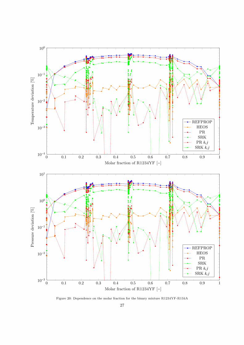
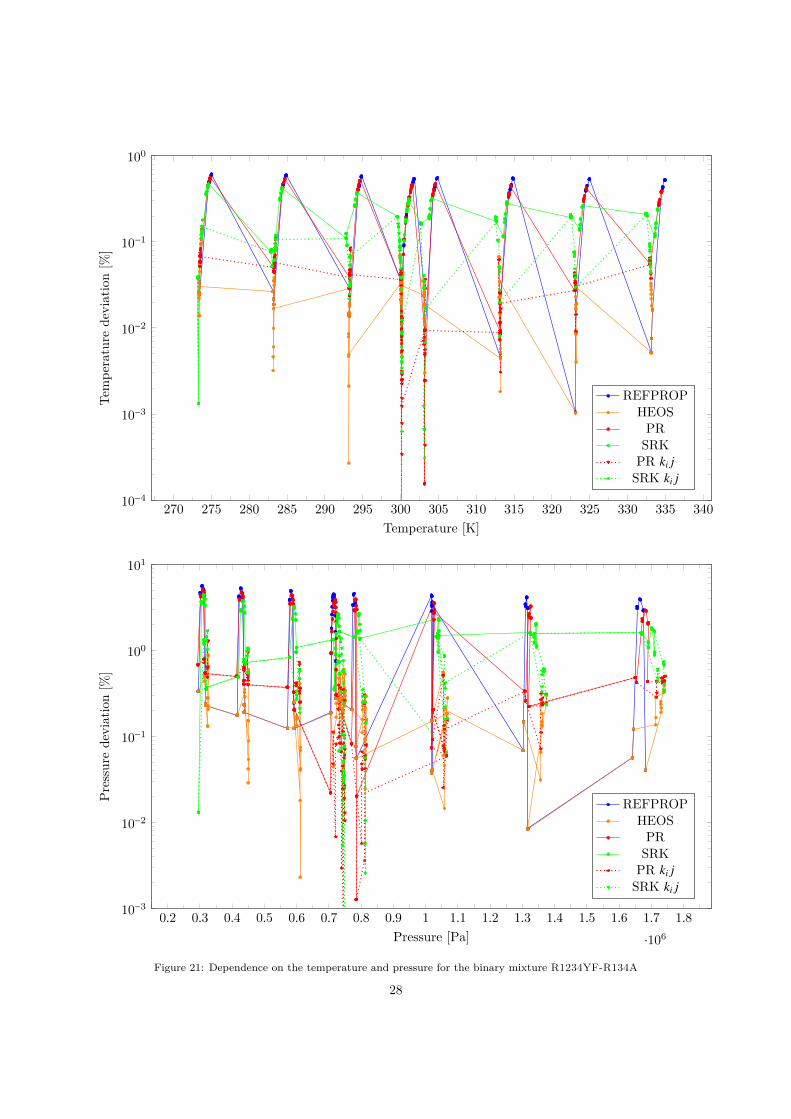
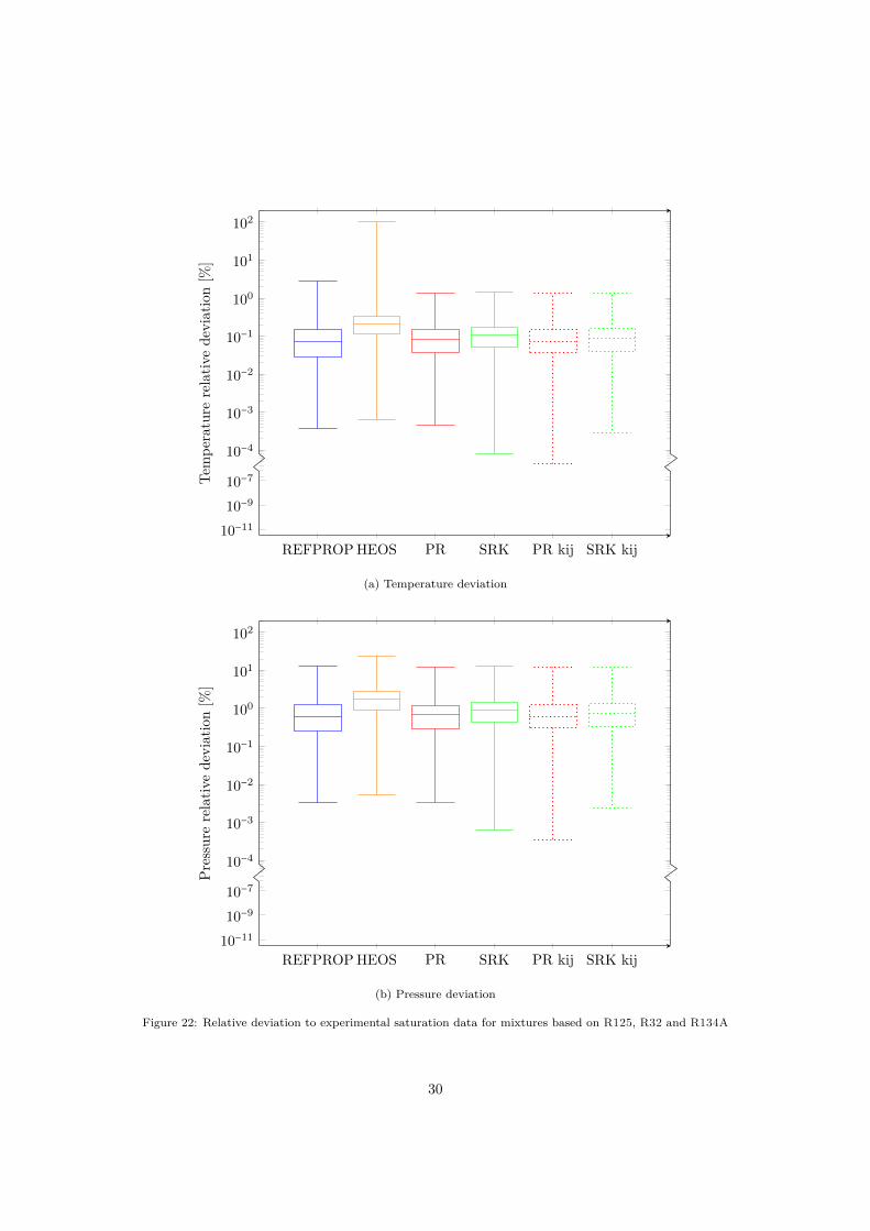
10minus4
10minus3
10minus2
10minus1
100
101
102
REFPROP HEOS PR SRK PR kij SRK kij10minus11
10minus9
10minus7Tem
pera
ture
rela
tive
devi
atio
n[
]
(a) Temperature deviation
10minus4
10minus3
10minus2
10minus1
100
101
102
REFPROP HEOS PR SRK PR kij SRK kij10minus11
10minus9
10minus7
Pres
sure
rela
tive
devi
atio
n[
]
(b) Pressure deviation
Figure 22 Relative deviation to experimental saturation data for mixtures based on R125 R32 and R134A
30
200 210 220 230 240 250 260 270 280 290 300 310 320 330 340 35010minus4
10minus3
10minus2
10minus1
100
Temperature [K]
Tem
pera
ture
devi
atio
n[
]
REFPROPHEOS
PRSRK
PR ki jSRK ki j
minus02 0 02 04 06 08 1 12 14 16 18 2 22 24 26 28 3 32 34 36 38
middot106
10minus3
10minus2
10minus1
100
101
Pressure [Pa]
Pres
sure
devi
atio
n[
]
REFPROPHEOS
PRSRK
PR ki jSRK ki j
Figure 23 Dependence on the temperature and pressure for the ternary mixture R125-R32-R134A
31
5 Acknowledgements
I would like to thank the professor Sylvain Quoilin for having given to me the opportunity to make thismaster thesis abroad This was a very interesting experience which allowed me to practice English and meetan other culture
I have a big thank to give to the DTU team who took care of me in Denmark the professor FredrikHaglind and the two post doctorates Maria E Mondejar Montagud and Jorrit Wronski It was a realpleasure to work with them
I also thanks Ian Bell our contact at NIST who manage to provide us with the database and withoutwho CoolProp would not exist
32
6 Conclusions
The simple cubic equations of state do not always gives satisfying results to compute density This canhowever be mostly corrected with a simple translation coefficient requiring a single measurement of saturatedliquid and more complex translation models could potentially give more accurate results
The cubic equations of states are very effective at modelling the liquid vapour equilibrium competingwith well recognise software
Depending on the interaction between the fluid constituting the mixtures all models benefit from binaryinteraction knowledge This is sometimes integrated in the software but would generally be an issue withnot yet well studied mixtures A simple coefficient (to be determined experimentally or approximated) canbe used to improve greatly the results of cubic equations when the interaction between the fluids is signif-icant An alternative would be to approximate the interaction with the UNIFAQ model as it is done withthe VTPR Determination of models to approximate the binary interaction parameters depending on thetype of fluid used would be an interesting subject for complementary study
More complex models can be used for the attractive parameter like the Mathias-Copeman and the TWUequations They both require 3 supplementary parameters and are already implemented in CoolProp Theirimpact could be interesting for a further study
The speed of the models are not compared in this work The comparison would be interesting butit is useful to notice CoolProp also provide a tabular interface which allows for extremely fast propertiescomputation when the tables have been generated (with a small loss of accuracy)
The cubic equations of states gives a wide range of possibilities from the simplest and fast model butslightly lacking accuracy to more complex and accurate models They provide a great tool for evaluation offluids when few data are available
33
Ahlers J Gmehling J 2001 Development of an universal group contribution equation of state Prediction of liquid densitiesfor pure compounds with a volume translated Peng-Robinson equation of state Fluid Phase Equilibria 191 (1-2) 177ndash188URL httpwwwsciencedirectcomsciencearticlepiiS0378381201006264pdfftmd5=86daea9e53bace87587e62b056b3007eamppid=1-s20-S0378381201006264-mainpdf
Bell I Jaumlger A 2016a Helmholtz energy transformation of common cubic equations of state for use with pure fluids andmixtures Journal of Research of the National Institute of Standards and Technology 121 (July) 238ndash263URL httpswwwresearchgatenetpublication304186500_Helmholtz_Energy_Transformations_of_Common_Cubic_Equations_of_State_for_Use_with_Pure_Fluids_and_Mixtures
Bell I H Jaumlger A 2016b Intermediate Terms 1ndash14Bell I H Jaumlger A 2016c Supplementary Information to accompany Helmholtz energy transformations of common cubic
equations of state for use with pure fluids and mixtures No 5Chen W-Y Liu J 2007 Mathcad Modules for Supercritical Fluid Extraction based on Mixing Rules Appendix A - Mixing
Rules (662) 1ndash10URL httphomeolemissedu~cmchengsExtractionAppendixA_MixingRulesdoc
CoolProp 2016 Cubic Equations of StateURL httpwwwcoolproporgcoolpropCubicshtml
Fauacutendez C a Valderrama J O 2009 Low pressure vaporndashliquid equilibrium in ethanol+congener mixtures using theWongndashSandler mixing rule Thermochimica Acta 490 (1-2) 37ndash42URL httpwwwsciencedirectcomsciencearticlepiiS0040603109000999pdfftmd5=65533f85d53569eeebae29e565402cc4amppid=1-s20-S0040603109000999-mainpdf
Frey K Augustine C Ciccolini R P Paap S Modell M Tester J 2007 Volume translation in equations of state as ameans of accurate property estimation Fluid Phase Equilibria 260 (2) 316ndash325URL httpwwwsciencedirectcomsciencearticlepiiS0378381207004591pdfftmd5=c750d4ea93f662a13b87183c76a8654eamppid=1-s20-S0378381207004591-mainpdf
Ji W-R Lempe D 1997 Density improvement of the SRK equation of state Fluid Phase Equilibria 130 (1-2) 49ndash63URL httpwwwsciencedirectcomsciencearticlepiiS0378381296031901
Lemmon E W Huber M L McLinden M O 2013 Reference Fluid Thermodynamic and Transport Properties-REFPROPversion 91URL httpwwwnistgovsrduploadREFPROP9PDF
Loacutepez J A Cardona C A 2006 Phase equilibrium calculations for carbon dioxide+n-alkanes binary mixtures with theWongndashSandler mixing rules Fluid Phase Equilibria 239 (2) 206ndash212URL httpwwwsciencedirectcomsciencearticlepiiS0378381205004565
Martin J J 1967 Equations of StatemdashApplied Thermodynamics Symposium Industrial amp Engineering Chemistry 59 (12)34ndash52URL httpdxdoiorg101021ie50696a008$delimiter026E30F$nhttppubsacsorgdoipdf101021ie50696a008
Martin J J 1979 Cubic Equations of State-Which Industrial amp Engineering Chemistry Fundamentals 18 (2) 81ndash97URL httpdxdoiorg101021i160070a001
Meng L Duan Y Y Wang X D 2007 Binary interaction parameter kij for calculating the second cross-virial coefficientsof mixtures Fluid Phase Equilibria 260 (2) 354ndash358URL httpwwwsciencedirectcomsciencearticlepiiS0378381207004323pdfftmd5=e3b19d08e08099003d28392a4450f768amppid=1-s20-S0378381207004323-mainpdf
Peng D-Y Robinson D B 1976 A New Two-Constant Equation of State Industrial amp Engineering Chemistry Fundamentals15 (1) 59ndash64URL httppubsacsorgdoiabs101021i160057a011
Schmid B Gmehling J 2012 Revised parameters and typical results of the VTPR group contribution equation of stateFluid Phase Equilibria 317 110ndash126URL httpdxdoiorg101016jfluid201201006
Schmid B Schedemann A Gmehling J 2014 Extension of the VTPR group contribution equation of state Groupinteraction parameters for additional 192 group combinations and typical results Industrial and Engineering ChemistryResearch 53 (8) 3393ndash3405
Soave G 1972 Equilibrium constants from a modified Redlich-Kwong equation of state Chemical Engineering Science 27 (6)1197ndash1203URL httpacels-cdncom00092509728009641-s20-0009250972800964-mainpdf_tid=cd3fc6c8-1dbd-11e6-a8de-00000aacb35dampacdnat=1463661351_8f1dbe034b52854e2d97cd6d80b7b56b
Valderrama J O 2003 The State of the Cubic Equations of State Industrial amp Engineering Chemistry Research 42 (8)1603ndash1618URL httppubsacsorgdoiabs101021ie020447b
Valderrama J O Marambio L E Silva A a 2002 Mixing rules in cubic equations of state applied to refrigerant mixturesJournal of Phase Equilibria 23 (6) 495ndash501URL httpdownloadspringercomstaticpdf558art3A1013612F105497102770331181pdforiginUrl=httplinkspringercomarticle101361105497102770331181amptoken2=exp=1463652668~acl=staticpdf558art253A101361252F105497102770
Wong D S H Sandler S I 1992 A Theoretically Correct Mixing Rule for Cubic Equations of State 38 (5)URL httponlinelibrarywileycomdoi101002aic690380505epdf
34
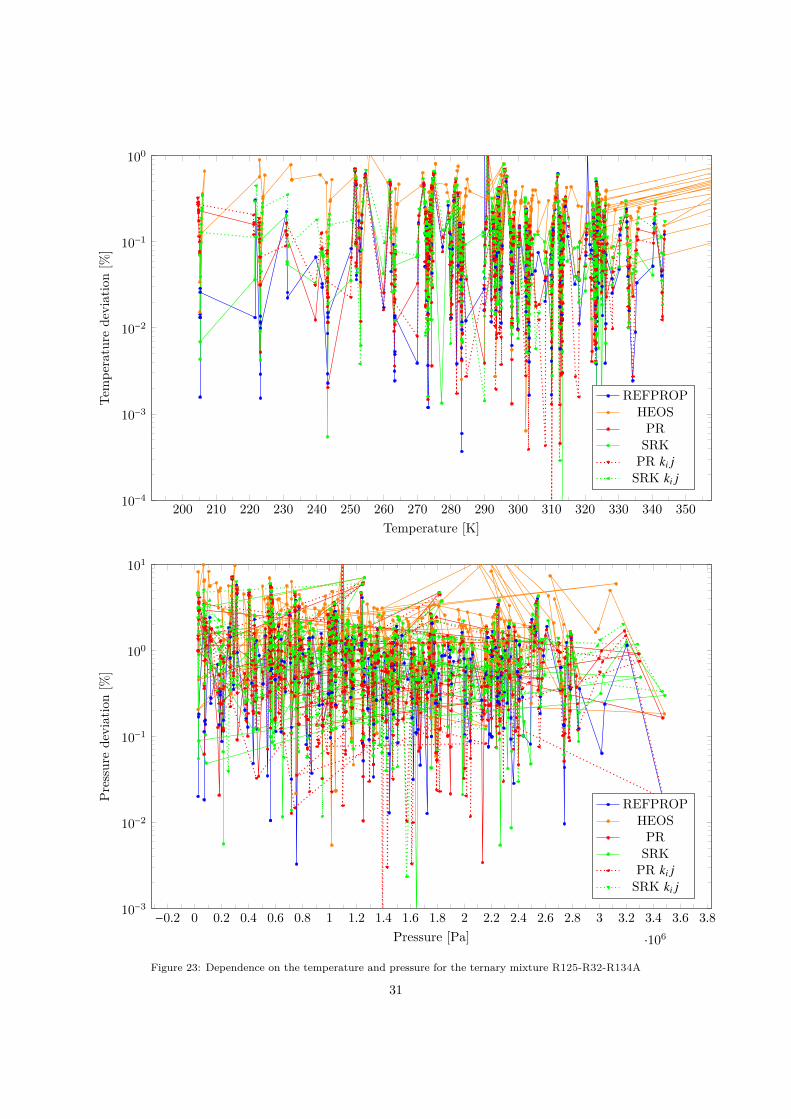