Locking-free adaptive mixed �nite elementmethods in linear elasticityDedicated to D. BraessC. Carstensen a G. Dolzmann b S. A. Funken a D. S. Helm aaMathematisches Seminar, Christian-Albrechts-Universit�at zu KielLudewig-Meyn-Str. 4, D-24098 Kiel, FRG.Email: fcc,saf,dshg@numerik.uni-kiel.debMax Planck Institute for Mathematics in the Sciences, Inselstr. 22-26, D-04103Leipzig. FRG. Email: georg@mis.mpg.deAbstractMixed �nite element methods such as PEERS or the BDMS methods are designedto avoid locking for nearly incompressible materials in plane elasticity. In this paper,we establish a robust adaptive mesh-re�ning algorithm that is rigorously based ona reliable and e�cient a posteriori error estimate. Numerical evidence is providedfor the �-independence of the constants in the a posteriori error bounds and for thee�ciency of the adaptive mesh-re�ning algorithm proposed.Key words: a posteriori error estimates, adaptive algorithm, reliability, mixed�nite element method, locking1 IntroductionIn this paper we investigate �nite element solutions of the Lam�e system inlinear elasticity and consider a plane elastic body with reference con�gura-tion � R2 and boundary @ = � = �D [ �N , �D 6= ;, �N = �n�D.Given a volume force f : ! R2 and a traction g : �N ! R2, we seek (anapproximation to) the displacement �eld u : ! R2 and the stress tensor� : !M2�2sym := f� 2M2�2 : � = � tg satisfying�div�= f; (1.1)�= C "(u) in ; (1.2)u=0 on �D; (1.3)�n= g on �N ; (1.4)Preprint submitted to Elsevier Preprint 29 July 1998

where "(v) = 12(rv + (rv)t) is the linearised Green strain tensor and� = �tr("(u))Id + 2�"(u); (1.5)is the Cauchy stress tensor (under the plain strain hypothesis). For positiveLam�e constants � and �, the fourth order elasticity tensor C is symmetric,bounded, and positive de�nite; tr(A) = A11 + A22 is the trace of the matrixA and Id is the 2� 2 unit matrix. As a consequence of Korn's inequality andthe Lax-Milgram lemma, problem (1.1){(1.4) has a unique solution (�; u) 2L2(;M2�2sym )�W 1;2()2.For nearly incompressible materials, i.e., for a Poisson ration � near to 1=2,the Lam�e constant � is very large and the standard computation of a �niteelement solution uh which is based on a displacement formulation (where (1.5)is used to substitute � in (1.1) and (1.4)) fails: The constant C(�) in the errorestimatejjC 1=2"(u� uh)jj2; � C(�)h� (1.6)(for small mesh-sizes h) tends to in�nity as �!1. To illustrate this lockinge�ect, Figure 1 displays the energy error vs mesh-size of numerical results forsix sequences of uniform meshes with six di�erent Poisson ratios �. For each �,an entry � is given at the position (pN; jjC 1=2"(u� uh)jj2;) for a mesh withN degrees of freedoms. The decription of the underlying test example will begiven below in Section 6. Note that we have a logarithmic scaling on bothaxes and so we observe from Figure 1 that the empirical convergence rate � isapproximately 0:5445 which is the (negative) slope of the a�ne interpolationof the data points. This is in agreement with theoretical predicitions becausethe exact solution has a singularity at the re-entering corner of the domain. The dependence of the constant in (1.6) suggests C(�) / 1=(0:5 � �) / �:Multiplication of � by 10 increases the error by a factor 3:16 � p10.Mixed �nite element formulations are designed for a robust approximation, i.e.,the constant C(�) in an error estimate as (1.6) is then �-independent. Stablenumerical schemes are obtained by relaxing the symmetry of the discrete stresstensor �h [19,8,2,21]: We seek (an approximation to) u : ! R2, � : !M2�2 and : !M2�2skew := f� 2 M2�2 : � + �t = 0g satisfying� = C (ru � ); � = �t; �div� = f in ;u = 0 on �D; �n = g on �N : (1.7)We refer to Section 2 for a variational formulation and its discretization whichyields the approximation (�h; uh; h) 2 �g;h�Uh�Wh with respect to PEERS(plane elasticity element with reduced symmetry) [2] and a modi�cation of the2

100

101

102

10−4

10−3

10−2

10−1

100

ν=0.3−0.45

ν=0.49

ν=0.499

ν=0.4999

ν=0.49999

1

0.5445

sqrt(N)

Err

or in

the

ener

gy n

orm

E=100000

sqrt(N)

Err

or in

the

ener

gy n

orm

Fig. 1. Energy norm of P1-displacement FE approximation error on the uniformmesh in Example 6.1 vs degrees of freedom N .BDM element BDMk due to Stenberg which we will therefore refer to asBDMSk element.The practical performance of the PEERS is robust in the sense that, at leastfor very small mesh-sizes, the error is (almost) independent of the crucialparameter � ! 1=2. This is supported by Figure 2 where we display numericalresults for the lowest order PEERS in Example 6.1 (compare with Figure 1).10

110

210

−4

10−3

10−2

10−1

100

1

1

ν=0.3−0.49999

1

0.5445

sqrt(N)

Err

or in

the

ener

gy n

orm

E=100000

adaptive uniform

sqrt(N)

Err

or in

the

ener

gy n

orm

Fig. 2. PEERS approximation error on uniform and adaptive meshes in Example6.1 vs degrees of freedom. (Energy norm of the stress errors.)In the example, a corner singularity reduces the convergence rate from theoptimal value 1 to � = 0:5445. This paper aims to improve such a poor con-vergence rate by proposing a robust mesh-re�ning algorithm for an e�cientautomatic mesh-design. In contrast to the ansatz in [6], our algorithm is rig-orously based on an e�cient and reliable a posteriori error estimate in natural3

norms established in [12] and proved with methods from [1,10].Given the discrete solution (�h; uh; h) and an element T in the triangulationTh, we compute�2T := h2T�2 jjf + div�hjj22;T + h2T jjcurl (C �1�h + h)jj22;T+ 1�2 jjAs (�h)jj22;T + hEjj h(C �1�h + h)tEi jj22;@Tn�+ hEkg � �hnk22;@T\�N + hEjj h(C �1�h + h �ruD)tEi jj22;@T\�D: (1.8)Here, hT is the diameter of T and E is an edge of T with length hE and [�]denotes the jump of the indicated quantity over an inner-element edge E. (SeeSection 3 for a detailed notation.) Notice that all terms are residuals: f+div�his the residual of (1.1), curl (C �1�h+ h) and [(C �1�h + h)tE] are residuals ofC �1�+ = ru (since the curlru = 0 and @u=@s = ru�tE = 0), As (�h) is theresidual to As� = 0, and the remaining terms are their modi�cations on theboundary of the domain. Then the proposed mesh-re�ning algorithm generatesa sequence of meshes and related Galerkin solutions. The corresponding errorsare shown in Figure 2.Adaptive Algorithm (A).(a) Start with coarse mesh T0.(b) Solve discrete problem w.r.t. Tk.(c) Compute �T for all T 2 Tk.(d) Compute error bound �PT2Tk �(T )2�1=2 and terminate or goto (e).(e) Mark element T red i� �(T ) � 12 maxT 02Tk �(T 0).(f) Perform red-green-blue-re�nement to avoid hanging nodes, update meshand goto (b).We refer to [18,23] for details on red-green-blue re�nement procedures andcorresponding data handling.>From the numerical results in Figure 2, we conclude that our algorithm ise�cient (because the experimental convergence rate is improved to the optimalvalue 1) and robust (because the errors are almost independent of �!1).The remaining part of the paper is organised as follows. The discrete subspacesas well as the weak form to (1.7) are described in Section 2. The underlyinga posteriori error estimate is given in Section 3. The proof is given in Section 4for convenient reading and because, compared to [12], we use di�erent scalingswith the Lam�e constant �. This leads to an a posteriori estimatejjC 1=2(� � �h)jj2; � c1(XT2Th �2T )1=2 =: c1 �(�;Th) (1.9)4

where the constant c1 is independent of � and �. Since PEERS appears tobe not very frequently used in practise, we give some details of our Matlab-relisation in Section 5. The experimental results are presented and discussedin Section 6. In particular, we will see that the convergence behaviour inExample 6.1 can indeed be optimised by Algorithm (A).2 Mixed �nite elementsIn the mixed variational formulation one seeks (�; u; ) 2 �g � U �W suchthat a(�; � ) + b(� ;u; ) = 0 and b(�; v; �) = �(f; v); (2.1)for all (�; v; �) 2 �0 � U � W. Here, the linear and bilinear forms and thefunction spaces �t, U , W are de�ned for t = 0 and t = g bya(�; � )= Z C �1� : �dx;b(�;u; )= Z �u � div� + � : �dx;(f; v)= Z f � vdx;�t= f� 2 L2(;M2�2) : div� 2 L2(;Rd); �n = t on �Ng;U �W =L2(;Rd)� L2(;M2�2skew):In this approach, the symmetry of the stress tensor � is relaxed and onlyimposed by means of the Lagrange multiplier . For �t;h, Uh, Wh �nite di-mensional spaces approximating �t, U , and W we de�ne the discrete solution(�h; uh; h) 2 �g;h � Uh �Wh bya(�h; �h) + b(�h;uh; h) = 0 and b(�h; vh; �h) = �(f; vh) (2.2)for all (�h; vh; �h) 2 �0;h � Uh �Wh. In this formulation, �h satis�es only theweak symmetry conditionZ �h : hdx = 0 ( h 2 Wh); (2.3)which does not imply �h = �th if �h � �th 62 Wh. In two dimensions, existence,uniqueness, and a priori estimates for several choices of discrete spaces havebeen proven in [21] which include the low order PEERS (plane elasticity ele-ment with reduced symmetry) constructed by Arnold-Brezzi-Douglas [2]5

and a modi�cation of the Brezzi-Douglas-Marini element BDMk due toStenberg (which we will refer to as BDMSk element).We assume that is a simply connected bounded domain in R2with polygonalboundary. Let Th be a regular triangulation of in the sense of [17], whichsatis�es the minimum angle condition, i.e., there exists a constant c2 > 0 suchthat c�12 h2T � jT j � c2h2T . Here, jT j is the area and hT is the diameter ofT 2 Th. The set of all element sides in Th is denoted by Eh and hE is thelength of the edge E 2 Eh. We assume in addition that �N is a �nite unionof connected components �i, i = 0; : : : ;M , and that �D has positive surfacemeasure. Thus we have Eh = E [ ED [ EN where E is the set of all interiorelement sides and ED and EN is the collection of all edges contained in �D and�N , respectively. We write E0h = E [ EN . It is useful to de�ne a function hThon by hTh jT = hT and a function hE on the union of all element sides byhE jE = hE.The de�nition of the �nite element spaces involves the bubble function bT =�1�2�3 on a triangle T 2 Th, where �i are the barycentric coordinates on T .The PEERS is based on the following function spacesUh= fvh 2 U : 8T 2 Th vhjT 2 P0(T )2g;Wh= f h 2 W \ C0(;M2�2skew) : 8T 2 Th hjT 2 P1(T ;M2�2skew)g;�h= f�h 2 L2(;M2�2) : div�h 2 U ;8T 2 Th �hjT 2 RT0(T )�B0(T )g;�t;h= f�h 2 �h : �hn = ~t on �Ng;where ~t is the L2(E)-projection of t onto P0(E)2 for all edges E � �N . Here,RT0 is the Raviart-Thomas space of lowest degree, andRT0(T )= f� 2 L2(T ;M2�2) : � = � + a x; � 2M2�2; a 2 R2g;B0(T )= f� 2 L2(T ;M2�2) : � = a Curl bT ; a 2 R2g;BDMk()= f�h 2 L2(;M2�2) : div�h 2 U ; �hjT 2 Pk(T ;M2�2)g:The higher order methods BDMSk are de�ned for k � 2 byUh= fvh 2 U : 8T 2 Th vhjT 2 Pk�1(T )2g;Wh= f h 2 W : 8T 2 Th hjT 2 Pk(T ;M2�2skew)g;�h= f�h 2 L2(;M2�2) : div� 2 U ;8T 2 Th �hjT 2 Pk(T ;M2�2)�Bk�1(T )g;�t;h= f�h 2 �h : �hn = ~t on �Ng;where ~t is the L2(E)-projection of t onto Pk(E)2, i.e., ~tjE := RE t ds=meas (E)6

if k = 0, andBk�1(T ) = f� 2 L2(T ;M2�2) : � = Curl (bTw); w 2 Pk�1(T )2g:3 A posteriori error estimateWe write u 2 Wm;p(Th) and v 2 Wm;p(Eh) if ujT 2 Wm;p(T ) for all T 2 Thand vjE 2 Wm;p(E) for all E 2 Eh. For each E 2 Eh we �x a normal nE to Esuch that nE coincides with the exterior normal to @ if E � @. Then,[v] jE := (vjT+)jE � (vjT�)jEif E = �T+ \ �T� and nE is the exterior normal to T+ on E and[v] jE = (vjT)jEif E = �T \ @. Finally we de�neCurl� = (�;2; ��;1) for � 2 W 1;2();Curlu = 0B@ u1;2 �u1;1u2;2 �u2;11CA ; curlu = u2;1 � u1;2;curl� = 0B@ �12;1 � �11;2�22;1 � �21;21CA ; div� = 0B@ �11;1+ �12;2�21;1+ �22;21CA :We use the standard notation for the Lebesgue spaces Lp() with norm k � kp;and the Sobolev spaces Wm;p() with norm k � km;p; and seminorm j � jm;p;.The closure of C1c (), the space of in�nitely often di�erentiable functionswith compact support, with respect to k � km;p; is denoted by Wm;p0 ().Theorem 3.1. Let Th be a shape-regular triangulation of � R2 and let(�h; uh; h) be the solution of (2.2) for the PEERS or the BDMSk element.Then there exists a �- and �-independent constant c3, which depends only on;�N ;�D and the polynomial degree of the elements, such that7

kC�1=2(� � �h)k2; � c3 �(�;Th) := c3 0@XT2Th �2T1A1=2 :Remark 3.1 (Displacement estimate). Amore general estimate is given in [12],ku� uhk2; + k � hk2; + kC �1=2(� � �h)k2;� c40@�(�;Th)2 + XT2Th h2T infvh2Uh kC �1�h + h �rvhk22;T1A1=2 : (3.1)Remark 3.2 (E�ciency). Assume in addition to the hypotheses of Theorem 3.1that curl (C �1�h+ h)jT is a polynomial for all T 2 Th and (���h)njE for allE � �N . Then there exists a constant c5, which depends only on , �, andthe polynomial degree of the elements, such that�(�;Th)� c5�ku� uhk2; + kC �1(� � �h) + � hk2;+k� � �hk2; + khTh(f + div�h)k2;�:Remark 3.3 (Volume contributions). As explained in [11], a Cl�ement-typeweakinterpolation can be used to re�ne Theorem 3.1. Indeed, the contributionXT2Th h2Tkcurl (C �1�h + h)k22;Tcould be replaced by a higher-order term.4 Proof of a posteriori error estimateThe proof is in the spirit of [1,10,12] and based on a Helmholtz decompositionof � � �h = sym(� � �h)� ' where sym(�) := [(�) + (�)t] =2 and ' := As (�h).De�ne v 2 H1D() := fv 2 H1()2 : v = 0 on �Dg as the solution toZ "(w) : C "(v) dx = Z "(w) : (� � �h) dx (w 2 H1D()): (4.1)Then, S := � � �h � C "(v) + ' 2 L2(;M2�2sym ) satis�esZ S : rwdx = 0 (w 2 H1D()) (4.2)and so, for j = 1; 2, (Sj1; Sj2) is divergence-free. According to classical resultsin potential theory, (Sj1; Sj2) is some Curl j, i.e., S = Curl for some 28

H1()2. We refer to [20,22] for details. Partial integration of (4.2) shows R�N w�Snds = 0. Since w is arbitrary on �N , Sn = 0, whence Curl n = 0 witht = (�n2; n1). This is r � t = 0, i.e., is constant on each component of �N .Because S = Curl is symmetric, 1;1+ 2;2 = 0 and so is divergence-free.Thus, = Curl� for some � 2 H2(). Altogether, cf. [12, Sect. 3],� � �h = C "(v) + Curl Curl�� ' where ' = As (�h):Therefore, the stress error is decomposed asZ C �1(� � �h) : (� � �h) dx = Z "(v) : (� � �h) dx+ ZCurl Curl� : C �1(� � �h) dx� Z ' : C �1(� � �h) dx (4.3)and we havekC�1=2(� � �h)k2; � kC �1=2CurlCurl�k2;+ kC 1=2"(v)k2; + kC �1=2'k2;: (4.4)Since C �1� = "(u) and since CurlCurl� is symmetric we haveZ CurlCurl� : C �1(� � �h) dx = Z CurlCurl� : (ru� C �1�h) dx: (4.5)Let 2 S1(Th) be constant on each component of �N and equal to there.The assumption on the trial space is �h := Curl 2 �0;h and so div �h = 0and (2.2) lead to Z C �1�h : �h dx = � Z �h : h dx : (4.6)Hence, Eqn. (4.5) leads toZ CurlCurl� : C �1(� � �h) dx= Z Curl ( �) : (� h � C �1�h) dx+ Z Curl : (� h � C �1�h) dx= � Z Curl ( �) : ( h + C �1�h) dx= Z( �) � curl h( h + C �1�h) dx+ Z[Eh( �) � h( h + C �1�h)tEi ds;(4.7)9

(curl h denotes the Th-piecewise curl operator). For any V 2 S0(Th)2, i.e., Vis Th-piecewise constant and possibly discontinuos, we computeZ "(v) : (� � �h) dx = Z "(v) : (� � �h +As (�h)) dx= Zrv : (� � �h +As (�h)) dx= Z�N v(g � �hn) ds+ Zrv : 'dx � Z(v � V ) � div(� � �h) dx� Z�N v(g��hn) ds� Z(v�V ) �div(���h) dx+kC �1=2'k2; kC 1=2rvk2;:(4.8)It follows from Korn's inequality that there is a constant c6 such thatkC 1=2rvk2; � c6kC 1=2"(v)k2;:>From Eqn. (4.3), (4.7), (4.8), (recall that hT resp. hE are mesh-sizes)kC�1=2(� � �h)k22; � kC �1=2'k2; kC 1=2rvk2;+q2�kh�1T (v � V )k2; 1=q2�khT div(� � �h)k2;+q2�kh�1=2E (v � ~V )k2;�N 1=q2�kh1=2E (g � �hn)k2;�N+ 1=q2�kh�1T ( �)k2;q2�khT curl h( h + C �1�h)k2;+ 1=q2�kh�1=2E ( �)k2;SEh q2�kh1=2E [( h + C �1�h)tE]k2;SEh+ kC �1=2'k2; kC �1=2(� � �h)k2;: (4.9)By Poincar�e's inequality with V being the elementwise integral mean of v, and~V jE the integral mean of vjE for an edge E � �N ,kh�1T (v � V )k2; � c7krvk2; (4.10)is bounded independently of the size of the elements. According to a weakinterpolation operator due to Cl�ement (see [7,16,17,11] and [13,14] for explicitbounds on c8 and c9) one can de�ne such thatkh�1T ( �)k2;+ kh�1=2E ( �)k2;SEh (4.11)� c8kr k2; = c8kCurl k2; ;kh�1=2E (v � ~V )k2;�N � c9krvk2;; (4.12)10

are bounded independently of the size of the elements. >From (4.9){(4.12), wededuce with Young's inequality, ab � a2=(2c) + b2c=2 for all a; b; c > 0,kC�1=2(� � �h)k22; � C c10�kC�1=2'k22; + 2�khT curl h( h + C �1�h)k22;+ 1=(2�)kh1=2E (g � �hn)k2;�N + 2�kh1=2E [( h + C �1�h)tE]k22;SEh+ 1=(2�)khT (f + div�h)k22;�+ c11=C �kC �1=2"(v)k22; + kC �1=2(� � �h)k22; + �=2kCurl k22;� (4.13)with C := 2c11c12 > 0 and constants c10; c11 > 0. A closer inspection ofkC �1=2Curl k2; adopting arguments from [9, page 199], showskCurl k22; � c122�kC �1=2Curl k22;: (4.14)>From this, Eqn. (4.4) yields the estimatec�113 kC �1=2(� � �h)k22; � khThcurl h(C �1�h + h)k22;+ kh1=2E h(C �1�h + h)tEi k22;E0h + khThdiv (� � �h)k22;+ kC�1=2As (�h)k22; + khE(g � �hn)k22;�N : (4.15)This concludes the proof.5 Matlab-Realization of PEERSIn this section we describe the Matlab implementation of PEERS with em-phasis on the sti�ness matrices which results in the global linear system ofequations Ax = b, namely0BBBBBBBBBBBB@ B C D E FC t 0 0 0 0Dt 0 0 0 0Et 0 0 0 0F t 0 0 0 0 1CCCCCCCCCCCCA0BBBBBBBBBBBB@x�xux x�Ex�F 1CCCCCCCCCCCCA = 0BBBBBBBBBBBB@ bDbf00bg 1CCCCCCCCCCCCA : (5.1)The symmetric and positive de�nite matrix B corresponds to the bilinearform a, C and D result from the bilinear form b. The continuity of stressvectors along inner edges is implemented through Lagrangian multipliers inthe matrix E for interior edges and F for edges on the Neumann boundary �N .The components x�, xu, x , x�E and x�F of the unknown vector x corrrespond11

to the basis of �h, Uh, Wh and to the Lagrange multipliers. The componentsbD, bf and bg re ect inhomogeneous Dirichlet boundary conditions, the volumeforce and applied surface forces. To approximate the integrals of the Dirichlet-conditions in the right hand side a 3-point-Gau�-quadrature is used.On a triangle T 2 Th with vertices P1, P2, P3 and center of mass s := (P1 +P2 + P3)=3 any discrete stress �h in �̂h,�̂h := f�h 2 L2(;M2�2) : 8T 2 Th �hjT 2 RT0(T )�B0(T )g;is of the form�h(x) = p + q (x� s) + r Curl bt = 8Xj=1 aj�j(x) (x 2 T ):Here p 2 R2�2 and q, r are coe�cient vectors in R2. The basis �1; : : : ; �8 weimplemented is shown in Table 1. The spaces for the Lagrangian multipliersare de�ned byMh= f� : �jE 2 P0(E)2; E � @T; T 2 T ; �jE = 0 for E � �Dg;Nh= f� : �jE 2 P0(E)2; E � �N ; �jE = 0 for E � �Dg:We chose (�1; �2) as a basis of Vh. The basis functions of Mh and Nh for theLagrange multipliers equal �1, �2 on the edge E and vanish elsewhere. Thebasis of the rotations in Wh is de�ned by �k, where, for each node zj, the hatfunction 'j is given by'j(zk)= �jk (k = 1; : : : ; card (K)); (5.2)card (K) denotes the cardinality of the nodes K. The components of the re-sulting sti�ness matrix B,Bjk := ZT (C �1�j) : �k dx (j; k = 1; : : : ; 8);12

Table 1Basis functions �1 = 0@ 1 00 11A �2 = 0@ 1 00 �11A�3 = 0@ 0 11 01A �4 = 0@ 0 �11 01A�̂h �5 = 0@ 111A (x� s)t �6 = 0@ 1�11A (x� s)t�7 = 0@ 111ACurl bt �8 = 0@ 1�11ACurl btUh �1 = 0@ 101A �2 = 0@ 011AMh; Nh �1 = 0@ 101A �2 = 0@ 011AWh �k = 0@ 0 'k�'k 0 1A (k = 1; 2; 3)are shown inB = jT j0BBBBBBBBBBBBBBBBBBBBBBB@2(� + 2�) 0 0 0 0 0 0 00 2� 0 0 0 0 0 00 0 2� 0 0 0 0 00 0 0 2� 0 0 0 00 0 0 0 B55 B56 0 � �300 0 0 0 B56 B66 �30 00 0 0 0 0 �30 B77 B780 0 0 0 � �30 0 B78 B88

1CCCCCCCCCCCCCCCCCCCCCCCA ;while the remaining coe�cients areB55 = �6 P3̀=1 jP` � sj2 + �12P2j;k=1P3̀=1(P`j � sj)(P`k � sk)t;B56 = �12P3̀=1((P`1 � s1)2 � (P`2 � s2)2);B66 = 2�+�12 P3̀=1 jP` � sj2 � �6 P3̀=1(P`1 � s1)(P`2 � s2);B77 = (2�+�)180 �P3j=1P2k=1 �2j;k�� �90 �P3j=1 �j;1�j;2� ;13

B78 = �180 ��P3j=1 �2j;1 +P3j=1 �2j;2� ;B88 = (2�+�)180 �P3j=1P2k=1 �2j;k�+ �90 �P3j=1 �j;1�j;2� :(Here, P`k (` 2 f1; 2; 3g; k 2 f1; 2g) denotes the k'th component of the `'thvertex of a triangle T 2 Th.)The bilinear form b(�i;�j; �k) results into two matrices C and D, with com-ponentsCjk = ZT �k � div�j dx (j = 1; : : : ; 8; k = 1; 2);Djk = ZT �j : �k dx (j = 1; : : : ; 8; k = 1; 2; 3):We obtain the local sti�ness matricesC = 2jT j0BBBBBBBBBBBBBBBBBBBBBBB@0 00 00 00 01 11 �10 00 0

1CCCCCCCCCCCCCCCCCCCCCCCA and D = 0BBBBBBBBBBBBBBBBBBBBBBB@0 0 00 0 00 0 0�23jT j �23jT j �23jT jD51 D52 D53D61 D62 D63D71 D72 D73D81 D82 D83

1CCCCCCCCCCCCCCCCCCCCCCCA ;where for j = 1; 2; 3D5j = jT j12 (Pjy � s2 � Pjx + s1);D6j = jT j12 (Pjy � s2 + Pjx � s1);D71 = 1120(P2y � P3y + P3x � P2x),D72 = 1120(P3y � P1y + P1x � P3x),D73 = 1120(P1y � P2y + P2x � P1x),D81 = 1120(P2y � P3y � P3x + P2x),D82 = 1120(P3y � P1y � P1x + P3x),D83 = 1120(P1y � P2y � P2x + P1x).14

The Lagrangian multipliers contribute to the matrices E and F , given byEjk = Fjk = � ZE �j � nE � �k dsfor j = 1; : : : ; 8; k = 1; 2 and an edge E = conv fP1; P2g � (E1; E2). Twoneighbouring elements T1; T2 with common edge E result in two matricesET1; ET2, whereET1 =0B@�E2 �E2 E1 �E1 � � 0 0E1 �E1 �E2 �E2 � 0 01CAtwith = (E2;�E1)�(P1�s). The matrix ET2 is then computed by ET2 = �ET1and using the center of mass of the triangle T2 instead of T1. For the Lagrangianmultipliers corresponding to the Neumann boundary only one matrix F of theform F = ET1 is necessary for every E � �N and neighbouring element T .6 Numerical ExamplesWe investigate three model problems of two-dimensional plain strain to pro-vide experimental evidence of the robustness, reliability and e�ciency of thea posteriori error estimate as the superiority of Algorithm (A) over a unifrommesh-re�ning.6.1 L-shaped domain with analytic solutionThe �rst model example on the L-shaped domain shown in Figure 3 modelssingularities arising at re-entrant corners. Using polar coordinates (r; �), �� <� � �, which are centered at the re-entrant corner, the exact solution u withradial component ur isur(r; �)= r�2� (�(�+ 1) cos((�+ 1)�) + (C2 � (�+ 1))C1 cos((�� 1)�));u�(r; �)= r�2� ((�+ 1) sin((� + 1)�) + (C2 + �� 1)C1 sin((� � 1)�)):The parameters are C1 = � cos((�+1)!)= cos((��1)!), C2 = 2(�+2�)=(�+�)where � = 0:54448373::: is the positive solution of � sin 2! + sin 2!� = 0 for! = 3�=4; the Young modulus is E = 100000 and the Poisson ratio varies inthe range 0:3 � � < 1=2). 15

4

21

ΓD

y

x

φrFig. 3. System and initial mesh in Example 6.1The standard FEM for the displacement formulation shows locking as shownFigure 1 and discussed in the introduction. The PEERS performs much betteras shown in Figure 2 for uniform meshes and in Figure 2 for automaticallygenerated meshes by Algorithm (A).In Table 4 the errors and the rates of convergence are displayed for � = 0:3. Fora mesh with N degrees of freedom, h := pN represents an averaged mesh-sizeand the energy error is jjj� � �hjjj = jjC�1=2(� � �h)jj2;. The experimentalconvergence rate (CR) is de�ned as a corresponding (negative) slope in Fig-ure 2; CR is shown in Table 4 and computed with the entries of the currentand the preceeding mesh.We observe that the experimental convergence rate tends to � which is ex-pected theoretically according to approximation results on uniform meshes ofsingular functions like u. The quotient jjj���hjjj=�(�;Th) of the energy normof the stress error and the a posteriori error bound �(�;Th) := (PT2Th �2T )1=2is seen to be nicely bounded from above and below. This con�rms numericallythat the a posteriori error estimate is h-independent.Table 4Errors and convergence rates (CR) on uniform meshes in Example 6.1 for � = 0:3.N h jjj� � �hjjj CR jju� uhjj2; CR jjj���hjjj�(�;Th)78 1.4142 0.007686 2.8676e-05 66.3309317 0.7071 0.006166 0.3142 1.4955e-05 0.9286 69.68941281 0.3536 0.004503 0.4501 7.5946e-06 0.9704 72.25365153 0.1768 0.003159 0.5094 3.8188e-06 0.9878 72.418420673 0.0884 0.002188 0.5284 1.9140e-06 0.9944 72.360782817 0.0442 0.001508 0.5362 9.5799e-07 0.9974 72.350016

Table 5 displays the ratio jjj���hjjj=�(�;Th) (which gives an estimate for c3)for di�erent values of h! 0 and �!1 in Example 6.1.Table 5Quotients for �=0.49999 for PEERS on uniform mesh in Example 6.1N h jjj���hjjj�(�;Th)78 1.4142 94.1275317 0.7071 79.81911281 0.3536 77.91295153 0.1768 76.435520673 0.0884 75.928282817 0.0442 75.765810

110

210

−6

10−5

10−4

10−3

ν=0.3−0.49999

1

1

sqrt(N)

η

E=100000

uniform adaptive

sqrt(N)

ηFig. 4. Error estimator � = �(�; Th) vs mesh-size pN in Example 6.1.In Figures 2, 4 and Table 6 we summarize the results of our computationswith Algorithm (A). The �nal mesh after 9 adaptive re�nements is shown inFigure 5.6.2 Cook's membrane problemAs a further test example we investigate a tapered panel clamped on oneend and subjected to a shearing load on the opposite end with f = 0 andg(x; y) = (0; 1000) if (x; y) 2 �N with x = 48 and g = 0 on the remaining partof �N as shown in Figure 6; E = 1 and � = 1=3. The linear elastic version17

Table 6Terms of the error estimator for � = 0:3 and uniform mesh re�nement:�2curl := XT2T h2T jjcurl (C�1�h + h)jj22;T , �2As :=PT2T h2T 1�2 jjAs(�h)jj22;T ,�2E := XE2E hE�jj �(C�1�h + h)tE� jj22;@Tn�+ jj �(C�1�h + h � ruD)tE� jj22;@T\�D+jjg � �hnjj22;�N�:N h �curl CR �As CR �E CR78 1.4142 3.5342e-05 9.4257e-06 1.0995e-04317 0.7071 3.8710e-05 -0.1298 1.3661e-05 -0.5293 7.8386e-05 0.48271281 0.3536 2.6029e-05 0.5684 1.0976e-05 0.3134 5.5559e-05 0.49295153 0.1768 1.7836e-05 0.5431 7.9072e-06 0.4712 3.9018e-05 0.507820673 0.0884 1.2316e-05 0.5331 5.5175e-06 0.5180 2.7068e-05 0.526582817 0.0442 8.4722e-06 0.5392 3.8165e-06 0.5312 1.8667e-05 0.5355−2 −1.5 −1 −0.5 0 0.5 1 1.5 2

−2.5

−2

−1.5

−1

−0.5

0

0.5

1

1.5

2

2.5

5

10

15

20

25

30

Fig. 5. Deformed mesh (left, displacements magni�ed by factor 2000) and vonMisesstress (right, with colour bar) plus a magni�ed detail of the neighbourhood of there-entering corner after 9 re�nements (N=12174) with Algorithm (A).of this simulation is often referred to as the Cook's membrane problem, andconstitutes a standard test for bending dominated response.Within 8 re�nement steps, Algorithm (A) generates a mesh and a stress ap-proximation displayed in Figure 7.The Figure 8 shows the vertical displacement of the top right corner vs thenumber of elements for two series of meshes, nameley for a uniform and andan adaptive mesh generated with Algorithm (A). We may conclude that theadaptively re�ned discretization is more e�cient than the uniform one and so18

DΓ

ΓN

48 mm

16 mm

44 mm

B

Fig. 6. Cook's membrane problem. System and initial mesh.0 10 20 30 40

10

20

30

40

50

60

0.05

0.1

0.15

0.2

0.25

0.3

0.35

0.4

0.45

0.5

Fig. 7. Deformed mesh (left, displacements magni�ed by factor 1=10) and von-Misesstress (right, with colour bar) plus a magni�ed detail of the neighbourhood of theupper left corner after 8 re�nements with Algorithm (A) for E = 1.the re�nement towards the top corner points appears reasonable.0 0.5 1 1.5 2 2.5

x 104

21

21.5

22

22.5

23

23.5

24

24.5

Number of elements

disp

lace

men

t in

y−di

rect

ion

at p

oint

B ν=1/3

E=1

uniform adaptive

Dis

plac

emen

t in

y-di

rect

ion

at p

oint

B

Number of ElementsFig. 8. Vertical displacement of the top corner point B vs number of elements.In comparison with the numerical results reported in [6], both adaptive schemesare of equaly good performance. The exact solution is unknown to the authors19

(the value for the exact displacement in Figure 8 was taken from [6]). To assesthe quality of the meshes, we therefore compute the error estimator �(�;Th)which is displayed in Figure 9. We observe for uniform and adapted meshesan experimental convergence rate 1 which is independent of the Poisson ratio�. The adaptive Algorithm (A) is signi�cantly better than a simple uniformdiscretization.10

110

210

310

−2

10−1

100

101

ν=0.3−0.49999

1

1

sqrt(dof)

η*

E=100000

uniform adaptive

η

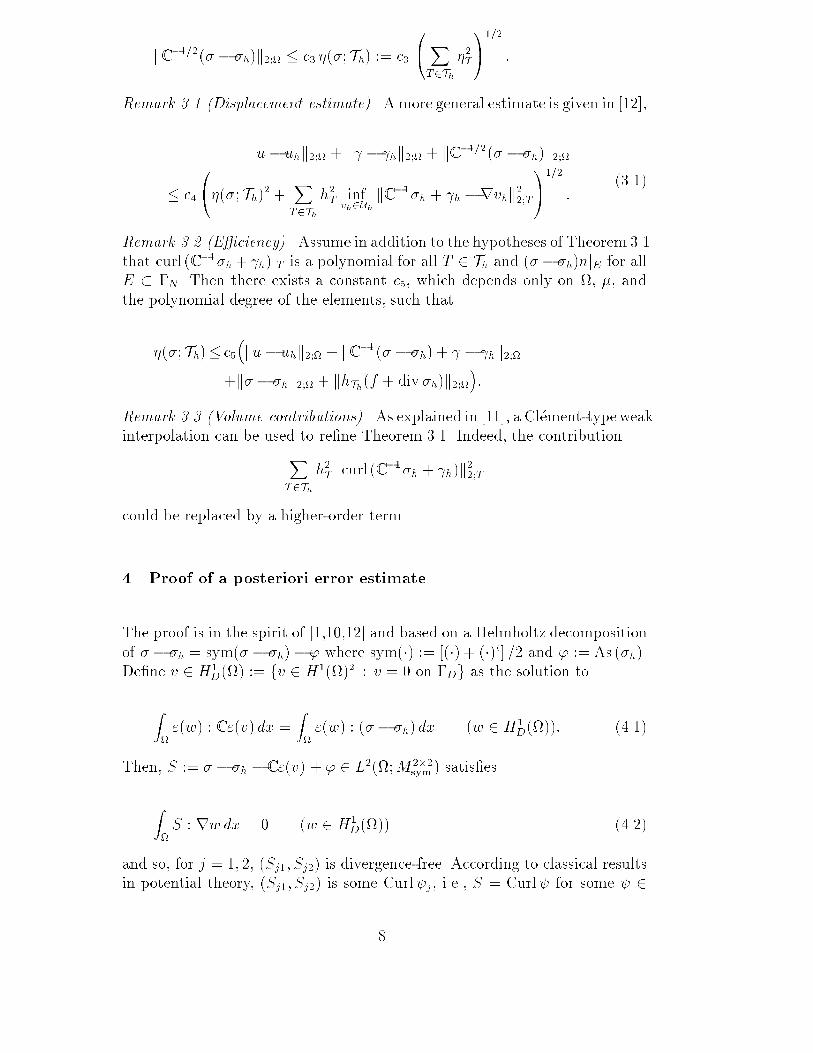
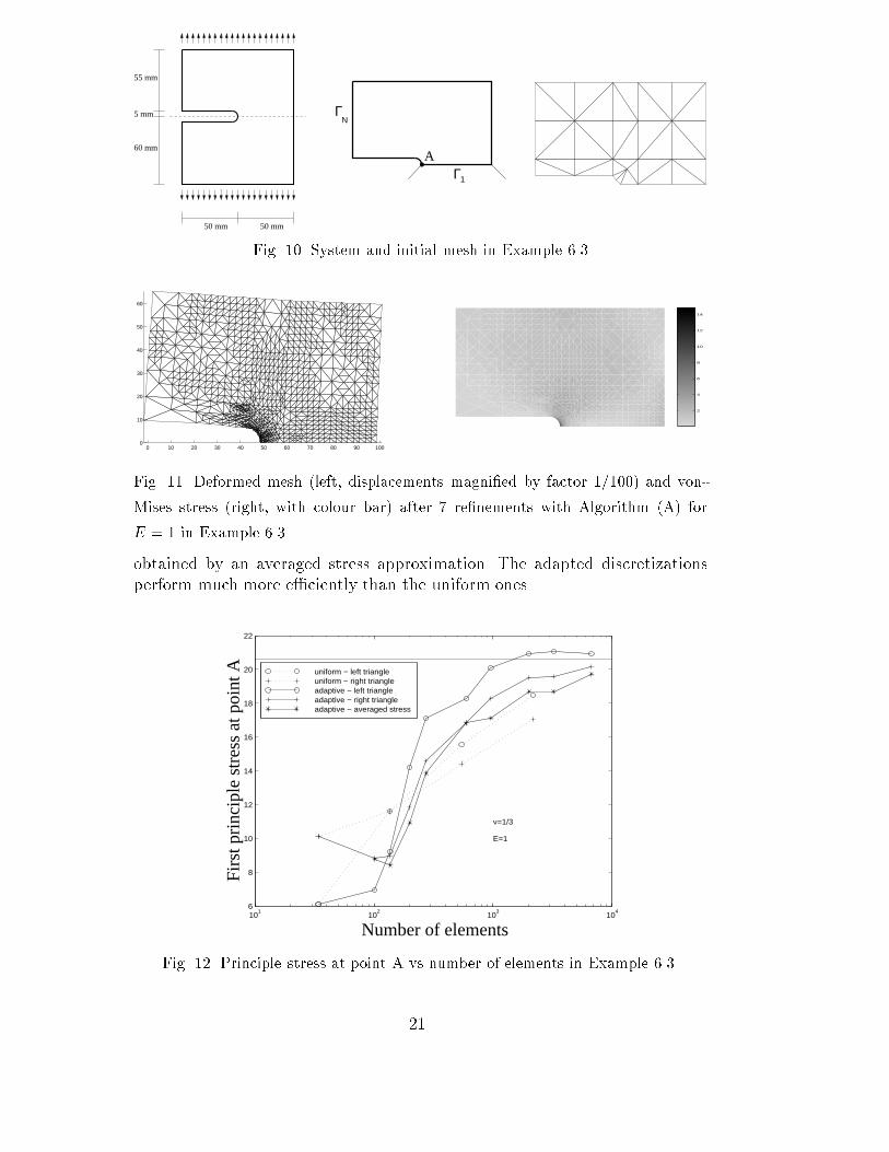
sqrt(N)Fig. 9. Error estimator � = �(�; Th) vs mesh-size pN in Example 6.2.6.3 Compact tension specimenA compact tension specimen, shown in Figure 10, is loaded with a surfaceload g = (100; 0) on �N (given by jyj = 60mm) and f = 0; E = 100000 and� = 1=3. The specimen is subjected to a vertical elongation or compression.As the problem is symmetric, one half of the domain was discretized. We �xedthe horizontal displacement with the constraint that the integral mean of allhorizontal displacements is zero.Within 7 re�nement steps, Algorithm (A) generates a mesh and a stress ap-proximation displayed in Figure 11. We observe a re�nement towards thecircular boundary near point A which appears reasonable as we might expecta smoothened singularity there.As a benchmark, we calculated the principal stress at point A displayed inFigure 12 (see Figure 10 for the location of A). Since point A is a node, itis unclear which triangle should contribute to the approximation. Hence, wedisplayed the values for the two triangles at that point and the approximation20

55 mm

50 mm 50 mm

60 mm

5 mm Γ

Γ1

Ν

AFig. 10. System and initial mesh in Example 6.30 10 20 30 40 50 60 70 80 90 100

0

10

20

30

40

50

60

2

4

6

8

10

12

14Fig. 11. Deformed mesh (left, displacements magni�ed by factor 1=100) and von-Mises stress (right, with colour bar) after 7 re�nements with Algorithm (A) forE = 1 in Example 6.3.obtained by an averaged stress approximation. The adapted discretizationsperform much more e�ciently than the uniform ones.10

110

210

310

46

8

10

12

14

16

18

20

22

Number of elements

Firs

t prin

cipl

e st

ress

at p

oint

A

ν=1/3

E=1

uniform − left triangle uniform − right triangle adaptive − left triangle adaptive − right triangle adaptive − averaged stress

Number of elements

Firs

t pri

ncip

le s

tres

s at

poi

nt A

Fig. 12. Principle stress at point A vs number of elements in Example 6.3.21

To asses the quality of the meshes, we displayed the error estimator � in Figure9 for various values of the Poisson ratio. Again, uniform and adapted meshesshow an experimental convergence rate 1 independently of the Poisson ratio�. Also, the adaptive Algorithm (A) yields signi�cantly better results than asimple uniform discretization.10

110

210

−4

10−3

10−2

ν=0.3−0.49999

1

1

sqrt(dof)

η*

E=100000

uniform adaptive

sqrt(N)

η

Fig. 13. Error estimator � = �(�; Th) vs mesh-size pN in Example 6.3.Acknowledgement: This paper has been initiated while G. Dolzmann visitedthe Mathematisches Seminar at the Christian{Albrechts{Universit�at zu Kiel,whose hospitality is gratefully acknowledged. D. S. Helm thanks the MaxPlanck Institute for Mathematics in the Sciences in Leipzig for two shortvisits.References[1] A. Alonso: Error estimators for a mixed method. Numer. Math. 74 (1996),385|395.[2] D.N. Arnold, F. Brezzi, J. Douglas: PEERS: A new �nite element forplane elasticity. Jap. J. Appl. Math 1 (1984) 347|367.[3] D.N. Arnold, R.S. Falk:Well-posedness of the fundamental boundary valueproblems for constrained anisotropic elastic materials. Arch. Ration. Mech.Anal. 98 (1987) 143|190. 22

[4] I. Babu�ska, W.C. Rheinboldt: Error estimates for adaptive �nite elementcomputations. SIAM Numer. Anal. 15 (1978) 736|754.[5] D. Braess: Finite Elements. Cambridge University Press (1997).[6] D. Braess, O. Klaas, R. Niekamp, E. Stein, F. Wobschal: Errorindicators for mixed �nite elements in 2-dimensional linear elasticity. Comput.Methods Appl. Mech. Engrg. 127 (1995), 345|356.[7] S.C. Brenner, L.R. Scott: The Mathematical Theory of Finite ElementMethods. Texts Appl. Math. 15, Springer, New-York (1994).[8] F. Brezzi, J. Douglas, L.D. Marini: Recent results on mixed �nite elementmethods for second order elliptic problems. In Vistas in applied mathematics.Numerical analysis, atmospheric sciences and immunology. Springer 1986[9] F. Brezzi, M. Fortin: Mixed and hybrid �nite element methods. Springer-Verlag (1991).[10] C. Carstensen: A posteriori error estimate for the mixed �nite elementmethod. Math. Comp. 66 (1997), 465|476.[11] C. Carstensen: Weighted Cl�ement-type interpolation and a posteriorianalysis for FEM. Berichtsreihe des Mathematischen Seminars Kiel, Technicalreport 97-19 Christian{Albrechts{Universit�at zu Kiel, Kiel (1997).[12] C. Carstensen, G. Dolzmann: A posteriori error estimates for the mixedFEM in elasticity. Numer. Math. in press (1998).[13] C. Carstensen, S.A. Funken: Constants in Cl�ement-interpolation errorand residual based a posteriori error estimates in Finite Element Methods.Berichtsreihe des Mathematischen Seminars Kiel, Technical report 97-11,Christian{Albrechts{Universit�at zu Kiel, Kiel (1997).[14] C. Carstensen, S.A. Funken: Fully reliable localised error control in theFEM. Berichtsreihe des Mathematischen Seminars Kiel, Technical report 97-12, Christian{Albrechts{Universit�at zu Kiel, Kiel (1997).[15] C. Carstensen, R. Verf�urth: Edge residuals dominate a posteriorierror estimates for low order �nite element methods. Berichtsreihe desMathematischen Seminars Kiel, Technical report 97-6, Christian{Albrechts{Universit�at zu Kiel, Kiel (1997). 23

[16] P. Cl�ement: Approximation by �nite element functions using localregularization. RAIRO S�er. Rouge Anal. Num�er. R-2 (1975) 77|84.[17] P.G. Ciarlet: The �nite element method for elliptic problems. North-Holland,Amsterdam (1978).[18]K. Eriksson, D. Estep, P. Hansbo, C. Johnson: Introduction to adaptivemethods for di�erential equations. Acta Numerica (1995) 105|158.[19] B.X. Fraeijs de Veubeke: Stress function appoach. In World congress onthe �nite element method in structural mechanics, Bournemouth (1975)[20]V. Girault, P.A. Raviart: Finite Element Methods for Navier-StokesEquations. Springer, Berlin (1986).[21] R. Stenberg: A family of mixed �nite elements for the elasticity problem.Num. Math. 53 (1988) 513|538[22] R. Temam: Theory and Numerical Analysis of the Navier-Stokes Equations.North-Holland (1977).[23] R. Verf�urth: A review of a posteriori error estimation and adaptive mesh-re�nement techniques. Wiley-Teubner (1996).

24