Elasticity of Demand for Sweetened and Unsweetened Drinks: The Case of Argentinian Households

 

F. Colella; I.R. Pace Guerrero

 

Argentinian Institute of Ag Technology, Economics Institute, Argentina

Corresponding author email: florencia.colella@outlook.com

Abstract:

Argentina is the fourth highest consumer of sweetened drinks, and the first consumer of soda in the world. In this paper we estimate a quadratic almost ideal demand system (QUAIDS) to explore demand for a number of sweetened and unsweetened beverages in Argentina. We use two household surveys: the last one available, performed in 2012-2013, and the previous one, carried over in 2004-2005. We explore expenditure shares and own and cross price elasticities. These results can shed light on a discussion that was held in 2017 in Congress towards the design of a tax reform on sweet beverages that will affect consumers, farmers, and the retail and food industries. Our results support the notion that a tax applied to highly sweetened beverages will affect consumption: for every 1% increase in price there will be a 1.32% drop in quantity purchased. In addition,we find that for every 1% price increase in highly sweetened beverages there will be a 1.12% increase in the amount of dairy beverages purchased.

Acknowledegment:

JEL Codes: Q18, D12

#1258 

1  

ELASTICITY OF DEMAND FOR SWEETENED AND UNSWEETENED DRINKS:

THE CASE OF ARGENTINEAN HOUSEHOLDS

Abstract

Argentina is the fourth highest consumer of sweetened drinks, and the first consumer of

soda in the world. In this paper we estimate a quadratic almost ideal demand system (QUAIDS)

to explore demand for a number of sweetened and unsweetened beverages in Argentina. We use

two household surveys: the last one available, performed in 2012-2013, and the previous one,

carried over in 2004-2005. We explore expenditure shares and own and cross price elasticities.

These results can shed light on a discussion that was held in 2017 in Congress towards the design

of a tax reform on sweet beverages that will affect consumers, farmers, and the retail and food

industries. Our results support the notion that a tax applied to highly sweetened beverages will

affect consumption: for every 1% increase in price there will be a 1.32% drop in quantity

purchased. In addition,we find that for every 1% price increase in highly sweetened beverages

there will be a 1.12% increase in the amount of dairy beverages purchased.

2  

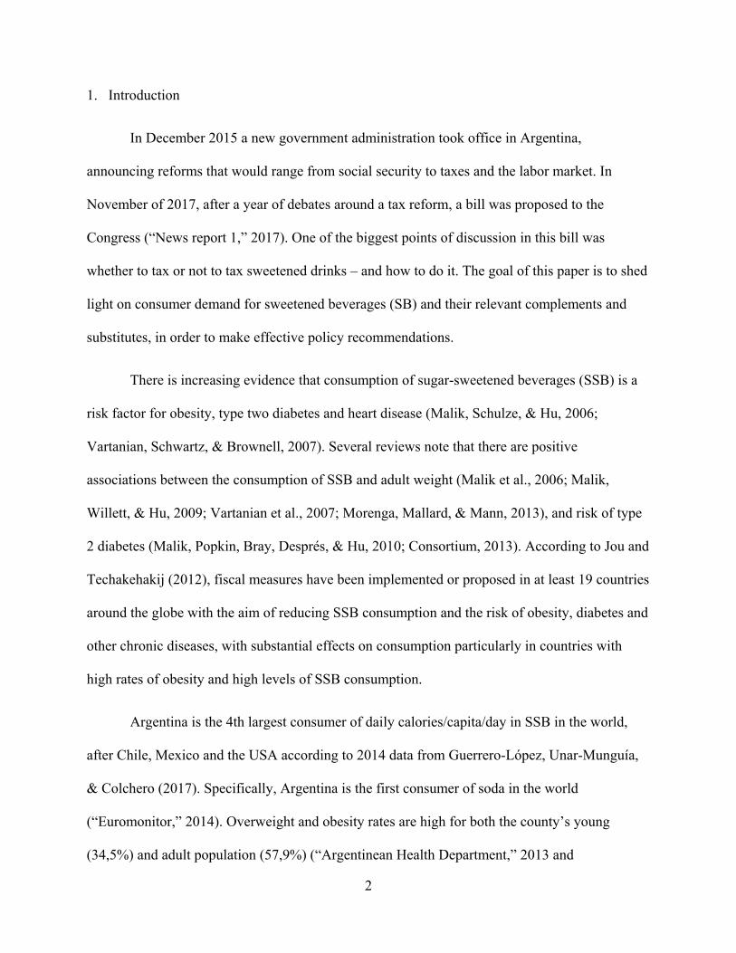
1. Introduction

In December 2015 a new government administration took office in Argentina,

announcing reforms that would range from social security to taxes and the labor market. In

November of 2017, after a year of debates around a tax reform, a bill was proposed to the

Congress (“News report 1,” 2017). One of the biggest points of discussion in this bill was

whether to tax or not to tax sweetened drinks – and how to do it. The goal of this paper is to shed

light on consumer demand for sweetened beverages (SB) and their relevant complements and

substitutes, in order to make effective policy recommendations.

There is increasing evidence that consumption of sugar-sweetened beverages (SSB) is a

risk factor for obesity, type two diabetes and heart disease (Malik, Schulze, & Hu, 2006;

Vartanian, Schwartz, & Brownell, 2007). Several reviews note that there are positive

associations between the consumption of SSB and adult weight (Malik et al., 2006; Malik,

Willett, & Hu, 2009; Vartanian et al., 2007; Morenga, Mallard, & Mann, 2013), and risk of type

2 diabetes (Malik, Popkin, Bray, Després, & Hu, 2010; Consortium, 2013). According to Jou and

Techakehakij (2012), fiscal measures have been implemented or proposed in at least 19 countries

around the globe with the aim of reducing SSB consumption and the risk of obesity, diabetes and

other chronic diseases, with substantial effects on consumption particularly in countries with

high rates of obesity and high levels of SSB consumption.

Argentina is the 4th largest consumer of daily calories/capita/day in SSB in the world,

after Chile, Mexico and the USA according to 2014 data from Guerrero-López, Unar-Munguía,

& Colchero (2017). Specifically, Argentina is the first consumer of soda in the world

(“Euromonitor,” 2014). Overweight and obesity rates are high for both the county’s young

(34,5%) and adult population (57,9%) (“Argentinean Health Department,” 2013 and

3  

“Argentinean Health Department,” 2012). Argentinean production of sweeteners – i.e. sugar plus

other sweeteners, except honey – has increased in the past 50 years, as shown in Figure 1

(“FAO,” 2013).

Figure 1: Argentinean production of sweeteners

Source: Elaborated with data from FAO, 2013

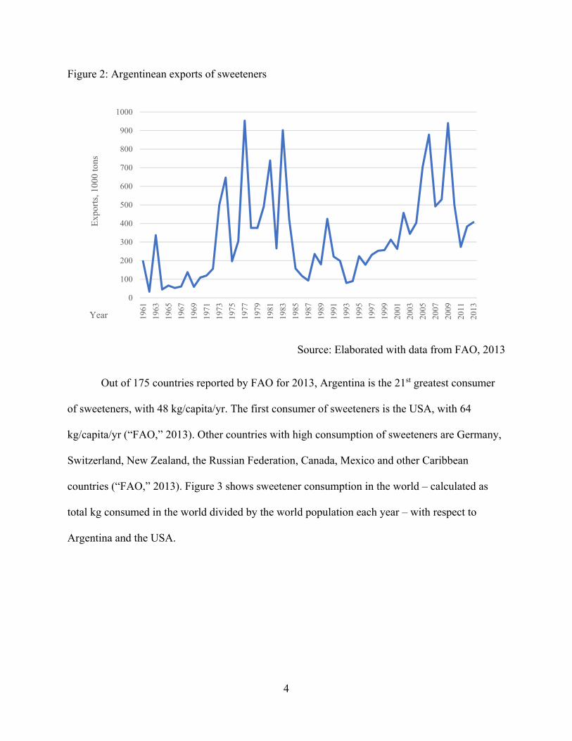
Argentinian exports of sweeteners ranked 34th out of 168 countries reported by FAO for

2013, presenting an increasing trend as shown in Figure 2. Argentinean imports of sweeteners, in

contrast, are very low, averaging 33,000 tons in the period 2003-2013 (“FAO,” 2013). This

amount represents 1.5% of the domestic supply, while exports were around 25% of the domestic

supply for that period (“FAO,” 2013). This suggests strong reliance from the industry in the

domestic market.

0

500

1000

1500

2000

2500

3000

1961

1963

1965

1967

1969

1971

1973

1975

1977

1979

1981

1983

1985

1987

1989

1991

1993

1995

1997

1999

2001

2003

2005

2007

2009

2011

2013

Pro

duci

on, 1

000

tons

Year

4  

Figure 2: Argentinean exports of sweeteners

Source: Elaborated with data from FAO, 2013

Out of 175 countries reported by FAO for 2013, Argentina is the 21st greatest consumer

of sweeteners, with 48 kg/capita/yr. The first consumer of sweeteners is the USA, with 64

kg/capita/yr (“FAO,” 2013). Other countries with high consumption of sweeteners are Germany,

Switzerland, New Zealand, the Russian Federation, Canada, Mexico and other Caribbean

countries (“FAO,” 2013). Figure 3 shows sweetener consumption in the world – calculated as

total kg consumed in the world divided by the world population each year – with respect to

Argentina and the USA.

0

100

200

300

400

500

600

700

800

900

1000

1961

1963

1965

1967

1969

1971

1973

1975

1977

1979

1981

1983

1985

1987

1989

1991

1993

1995

1997

1999

2001

2003

2005

2007

2009

2011

2013

Exp

orts

, 100

0 to

ns

Year

5  

Figure 3: Consumption of sweeteners in the world, Argentina and the USA

Source: Elaborated with data from FAO, 2013

The decrease in the USA’s consumption of sweeteners after 2006 that can be noted at the right

hand of Figure 3 was analyzed by Welsh, Sharma, Grellinger, & Vos (2011), who found that it

was driven by a reduction in soda consumption as compared to other sweet food products.

The bill introduced to the Congress in Argentina in 2017 was designed with the Pan

American and World Health Organizations’ (PAHO and WHO, respectively) sweetener

consumption recommendations in mind. The WHO and PAHO suggest implementing fiscal

measures to discourage the consumption of foods and beverages that can harm health. For

instance, the Plan of Action for the Prevention of Obesity in Children and Adolescents in the

Americas, presented by PAHO in 2014, advises taxing SSB and high-energy dense products in

order to stop the increase in the prevalence of obesity in children and adolescents (“PAHO,”

2014). The WHO recommendation is to not go over 50 grams per day for a 2,000 kcal diet

0

10

20

30

40

50

60

70

80

1961

1963

1965

1967

1969

1971

1973

1975

1977

1979

1981

1983

1985

1987

1989

1991

1993

1995

1997

1999

2001

2003

2005

2007

2009

2011

2013

Con

sum

ptio

n (k

g/ca

pita

/yr)

Year

Argentina

World

United Statesof America

6  

(“WHO,” 2015). The bill in discussion intends a tax proportional to the content of sweeteners in

a drink, applicable to SB with over 40 grams per liter, except for those containing over 20% of

natural juice, in which case the tax starts applying once the amount of sweetener exceeds 50

grams per liter.

Cabrera Escobar, Veerman, Tollman, Bertram, & Hofman (2013) analyzed nine articles

from the USA, Mexico, Brazil and France to assess the potential impact of taxes or price

increases on SB on consumption levels. They report that all the studies reviewed showed

negative own-price elasticity, and that the mean value is −1.2, implying that higher prices are

associated with a lower demand. Zhen, Wohlgenant, Karns, & Kaufman (2011) found that in the

USA a half-cent per ounce tax on SSB results in a moderate reduction in consumption in the

short run, but a 15 to 20% higher reduction in the long run due to habit formation. Dharmasena

& Capps (2012) looked into the consequences of a tax on SSB to combat the U.S. obesity

problem. They found that consumption of isotonics, regular soft drinks and fruit drinks is

negatively impacted by the tax, while consumption of fruit juices, low-fat milk, coffee, and tea is

positively affected. They suggest considering interrelationships among non-alcoholic beverages

in assessing the effect of a tax. Another study, performed by Pou et al. (2016), highlights that in

Argentina obesity is a recognized public health issue. However, this study could not confirm that

consumption of SSB is significantly linked to overweight and obesity. Another developing

country (neighbor to Argentina) where the demand for SSB was studied is Chile, the world

second largest per capita consumer of caloric beverages. In this study, Guerrero-López, Unar-

Munguía, & Colchero (2017) found that other food and beverages behave as substitutes for soft

drinks and that the demand for soft drinks is price sensitive. Therefore, an incentive system with

subsidies and/or taxes could lead to substitutions. Colchero, Salgado, Unar-Munguía, Hernández-

7  

Ávila, & Rivera-Dommarco (2015) analyzed the demand for beverages and high-energy food in

Mexico, and found that a price increase in soft drinks is associated with greater consumption of

water, milk, snacks and sugar; and a decrease in the consumption of other SB, candies and

traditional snacks. The same was found for the SB group except that an increase in price of SB

was associated with a decrease in snack consumption. They estimated the price elasticity of SB

in −1.16, and between −1.06 and −1.29 for soft drinks. They found higher elasticities among

lower income households, and they point out that the implementation of a tax could decrease

consumption particularly among the poor. They also note that substitutions and

complementarities with other food and beverages should be evaluated to assess the potential

impact on total calories consumed. In Ecuador, the price elasticity of SSB was reported to be

between −1.17 and −1.33 depending on the socioeconomic group (Paraje, 2016). Demand in

Argentina has been studied for meat (Monzani and Robledo, 2011; Pace Guerrero, Berges, &

Casellas, 2015), dairy (Rossini, Guiguet, & Villanueva, 2008) and food in general (Rossini &

Guiguet, 2008; Berges & Casellas, 2007; Lema et al., 2008); but as far as we know demand for

SB in comparison to other drinks has not been analyzed yet.

During the discussion on the bill that motivated this study, sugarcane producers and

representatives from the soda and juice industry stated that this tax would disproportionately

affect them. Fruit and corn producers were also concerned given their relationship to the juice

industry. This led to several representatives from different regions bringing the matter up in

Congress. Furthermore, Coca-Cola announced it would reverse planned investments for one

thousand million dollars along with juice purchases for another 250 million (“News report 2,”

2017). In a sensitive context, policymakers’ decisions must be informed. Assessing whether the

consumption of certain drinks or food products will change in response to variations in prices is

8  

valuable information. The goal of this study is to analyze the potential effect of a tax to SB in the

consumption of related products. Some questions we answer are: is the demand for various

beverages different across groups? What are the compensated and uncompensated demand cross

and own-price elasticities? Are these products substitutes or complements? What are the

expenditure elasticities of these products? Are they considered necessities or luxury goods? What

are their expenditure shares?

The rest of the paper is organized as follows: section 2 presents the methodology, section

3 describes de data, section 4 presents the results, and section 5 presents the main conclusions

and policy implications.

2. Methods

We use the quadratic almost ideal demand system (QUAIDS) developed by Blundell et al.

(1993) and Banks et al. (1997). The QUAIDS takes into account linear models such as the AIDS

by Deaton and Muellbauer (1980) or the Translog by Jorgenson and Lau (1975) but unlike them,

and by virtue of including a quadratic expression for the income variable, it fits the existence of

goods that behave as luxury goods at lower levels of income, and as necessities at higher ones.

The QUAIDS model also preserves all the qualities of the AIDS model, such as flexibility and

consistency in the aggregation of consumers.

The system is estimated using the expenditure/budget share for each good ( ), its price ( )

and the income or total expenditure ( ). The parameters to be estimated are , , and .

We assume weak separability of preferences. This means that preferences for products in a group

are independent from consumption of products in other groups, and the marginal rate of

9  

substitution between two products in one group is independent from quantities of goods

consumed in other groups (Deaton & Muellbauer, 1980). Therefore, we incorporate the total

expenditure in order to obtain a complete system of equations (i.e., to make the system reach the

budget restriction). In this paper, these separable groups are formed based on the type of drink,

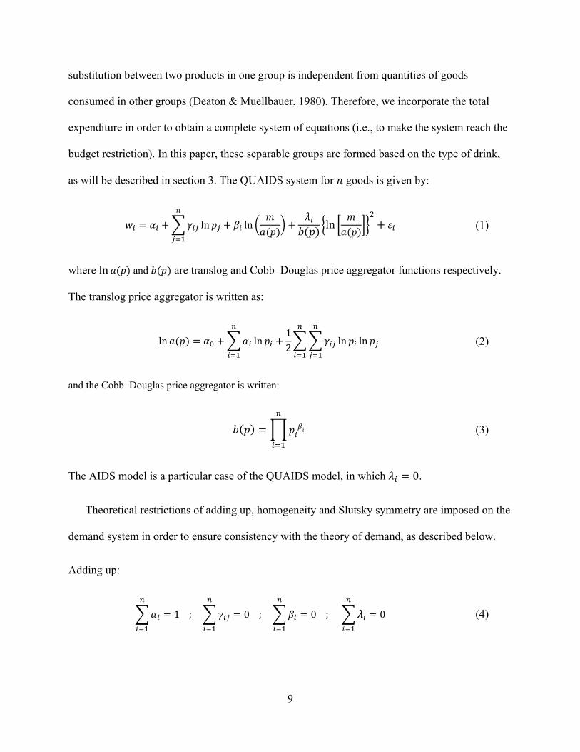
as will be described in section 3. The QUAIDS system for goods is given by:

ln ln ln2

(1)

where ln and are translog and Cobb–Douglas price aggregator functions respectively.

The translog price aggregator is written as:

ln ln12

ln ln (2)

and the Cobb–Douglas price aggregator is written:

(3)

The AIDS model is a particular case of the QUAIDS model, in which 0.

Theoretical restrictions of adding up, homogeneity and Slutsky symmetry are imposed on the

demand system in order to ensure consistency with the theory of demand, as described below.

Adding up:

1; 0 ; 0 ; 0 (4)

10  

Homogeneity:

0 (5)

Symmetry:

(6)

To calculate QUAIDS elasticities we derive equation 1 with respect to ln and ln

respectively, following Banks et al. (1997):

≡ln

2ln (7)

≡ln

ln ln2 (8)

The expenditure elasticities are then given by:

1 (9)

And the uncompensated price elasticities are given by:

(10)

where 0∀ and 1∀ .

Finally, the set of compensated elasticities are calculated using the Slutsky equation:

∗ (11)

11  

3. Data

The National Household Expenditure Survey (NHES) is conducted by the Argentinean

Institute of Statistics and Census (AISC). We use data from the last two surveys: 2004/05

(NHES1) and 2012/13 (NHES2).

The surveys collect household information on daily food and beverage quantities purchased

and expenses incurred during one week, as well as household socio-demographic data. Since

prices are not recorded directly, they are derived from household daily expenditures and

quantities purchased in liters. Prices are also deflated using the Consumer Price Index (CPI)

reported by AISC, using as base period the last month of data collection for each survey.

We look into 5 groups of goods: highly sweetened beverages (HSB), lightly sweetened

beverages (LSB), water, dairy beverages (DB) and infusions. Drinks with sweetener

concentrations such that the recommendations of the WHO are reached with less than 3 glasses

are considered HSB in this study. This comprises sodas and juices, according to the Inter-

American Heart Foundation (2014). LSB are those of which 3 to 5 glasses per day can be

consumed safely, according to WHO recommendations. In this group there are flavored waters,

isotonic drinks, herbal beverages and soybean drinks (“Inter-American Heart Foundation,”

2014). In the water group we include sparkling and plain water, mineral or not. In the DB group

we include milk and yoghurt drinks. In the infusions group we include coffee, tea, malt, cocoa

and yerba mate, a traditional local infusion.

3.1 Adjusting data for price quality

We calculate implicit prices, i.e. the ratio between the total expenditure and the purchased

quantity for each good or group of products. The introduction of these prices, however, poses

12  

additional problems due to the fact that they reflect “quality effects” that should be corrected

before the estimation. Variation of cross-sectional prices can be driven by differences in the

regions and price discrimination (changes in the supply); services acquired with the

commodities; seasonal effects and differences in the quality due to the aggregate of non-

homogeneous goods (Cox & Wohlgenant, 1986). Following Cox and Wohlgenant (1986), we

include these differences by adjusting the prices for each one of the groups to variables that fit

the appropriate “quality effect” for each household. The selected explanatory variables −

following Berges and Casellas (2007) − are shown in the following expression:

∗ 2 ⋯ 12 (12)

where indicates the implicit price for each group of goods; indicates the head of

household’s age; is a dummy variable that represents the gender of the head of

household (equals 1 if the head of household is a woman); and are dummy variables

that equal 1 if the head of household has a high school degree and college degree respectively;

refers to the number of members in the household; represents the total household

income, which is also included squared and multiplied by the size of the household;

represents the activity of the head of household (it is 1 if the head of household is employed);

and 2 to 12 are dummy variables, one for each sub-region. The quality-adjusted

price is then for households that reported expenditure in the goods considered, and plus the

estimated coefficient of the dummy variable indicating the sub-region ( 2 to 12) for

households with zero consumption.

13  

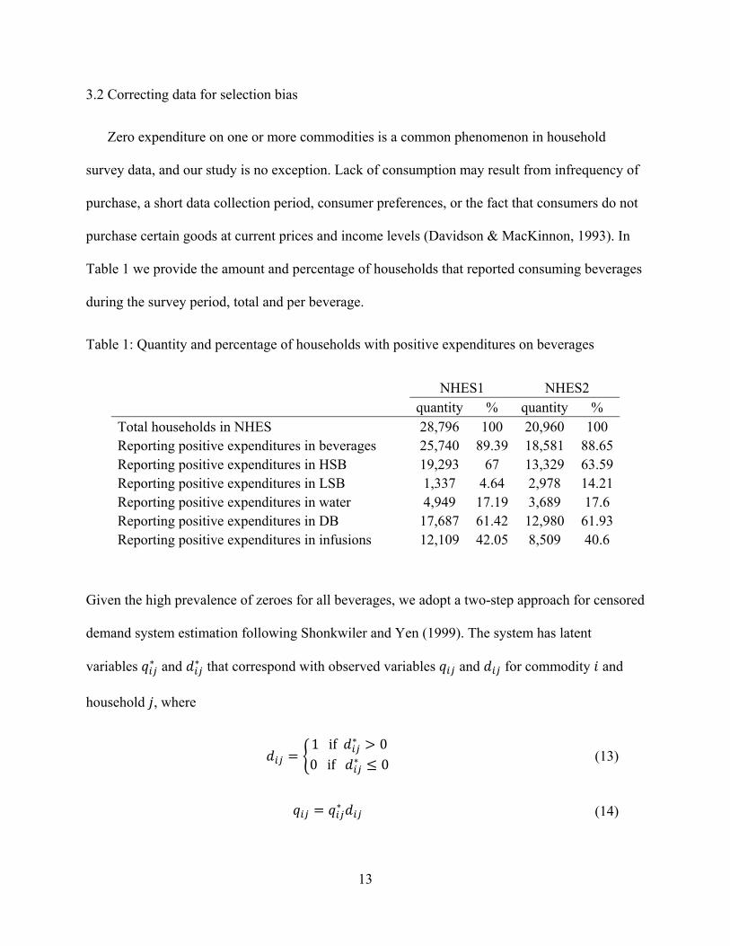
3.2 Correcting data for selection bias

Zero expenditure on one or more commodities is a common phenomenon in household

survey data, and our study is no exception. Lack of consumption may result from infrequency of

purchase, a short data collection period, consumer preferences, or the fact that consumers do not

purchase certain goods at current prices and income levels (Davidson & MacKinnon, 1993). In

Table 1 we provide the amount and percentage of households that reported consuming beverages

during the survey period, total and per beverage.

Table 1: Quantity and percentage of households with positive expenditures on beverages

NHES1 NHES2

quantity % quantity % Total households in NHES 28,796 100 20,960 100 Reporting positive expenditures in beverages 25,740 89.39 18,581 88.65Reporting positive expenditures in HSB 19,293 67 13,329 63.59Reporting positive expenditures in LSB 1,337 4.64 2,978 14.21Reporting positive expenditures in water 4,949 17.19 3,689 17.6 Reporting positive expenditures in DB 17,687 61.42 12,980 61.93Reporting positive expenditures in infusions 12,109 42.05 8,509 40.6

Given the high prevalence of zeroes for all beverages, we adopt a two-step approach for censored

demand system estimation following Shonkwiler and Yen (1999). The system has latent

variables ∗ and ∗ that correspond with observed variables and for commodity and

household , where

1 if ∗ 00 if ∗ 0

(13)

∗ (14)

14  

and

∗ ′ (15)

∗ , (16)

Variable represents the probability of household purchasing good , and takes the form of a

dichotomous variable that is equal to one if consumption is different from zero, and zero if

consumption is zero. Variable indicates the actual quantity consumed by those who chose to

consume. The observed quantity consumed will equal the latent quantity if the consumer is

actually purchasing the item ( 1 , and zero if not. . is an indicator function, ′ and

are vectors of observables, and are parameter vectors, and and are random error

terms. This model is a generalization of Amemiya’s (1974) system in which the censoring of

each dependent variable is governed by a separate stochastic process. Years later, Yen (2005)

and Yen and Lin (2006) suggested a censored two-step multivariate procedure that improved the

efficiency of the estimator. We use this two-step procedure in which the first stage is modeling

the probability of positive consumption using a Probit model and obtaining . − the

probability density function − and Φ . − the cumulative distribution function. If we assume that

the error terms , ′ follow a bivariate normal distribution with , , then the

conditional mean of is (Wales and Woodland, 1980):

, ; ′ ,Φ

(17)

15  

And because , ; ′ 0, the unconditional mean of is:

, Φ , (18)

Based on equation 18, the system of equations 13 to 16 can be rewritten as:

Φ , (19)

where , . We then obtain ML probit estimates of , using the binary

outcome for each . To do this, we use the same variables used in the estimation of implicit

quality-adjusted prices plus dummy variables for presence of people younger than 14 and older

than 65 in the household. Estimation of separate probit models instead of one multivariate probit

implies the restriction 0∀ . With some loss in efficiency relative to the

multivariate probit, the separate probit estimates are nevertheless consistent.

In the second step we calculate Φ and , and estimate , a vector of the

parameters in the QUAIDS ( , , , , and :

Φ , (20)

Because the ML probit estimators are consistent, applying ML or SUR estimation to equation

20 produces consistent estimates in the second step.

According to Shonkwiler and Yen’s (1999) method, the QUAIDS corrected for zero

consumption is then:

Φ ′ ln ln ln2

′ (21)

16  

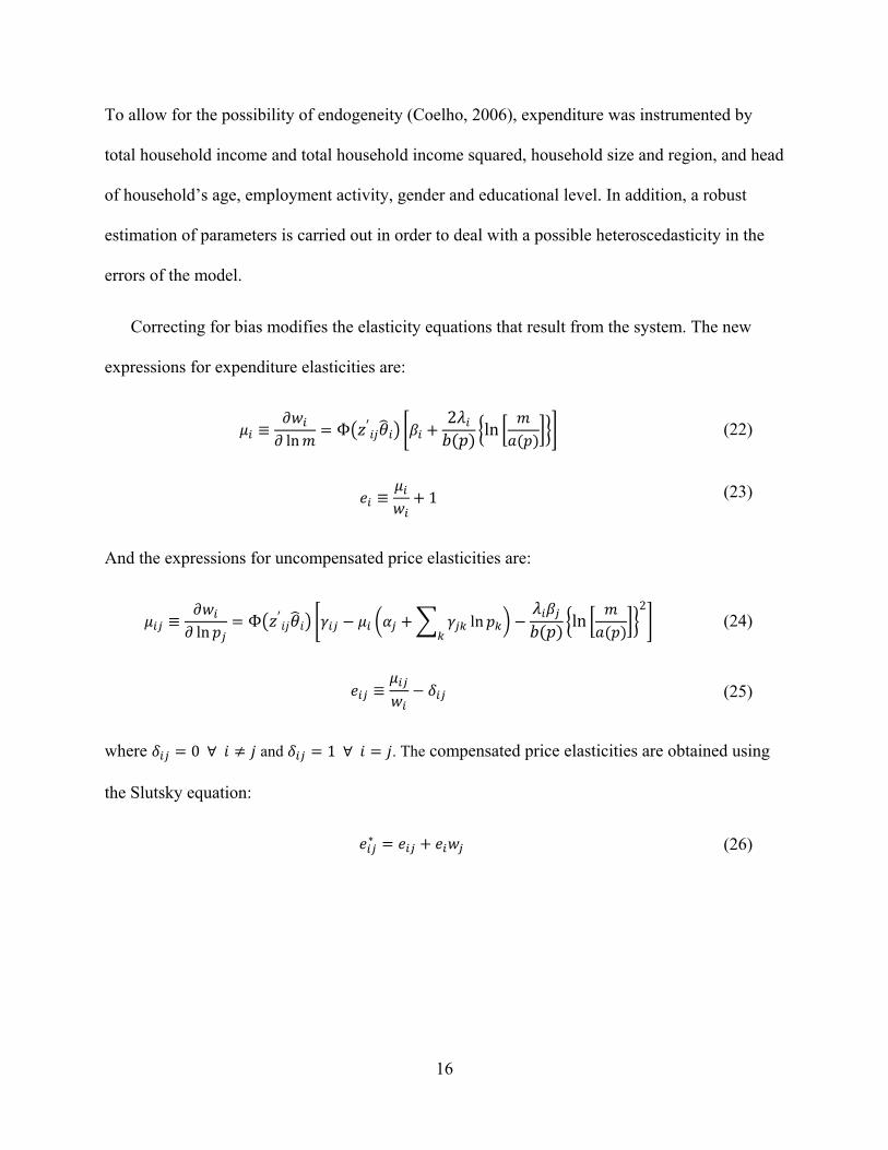
To allow for the possibility of endogeneity (Coelho, 2006), expenditure was instrumented by

total household income and total household income squared, household size and region, and head

of household’s age, employment activity, gender and educational level. In addition, a robust

estimation of parameters is carried out in order to deal with a possible heteroscedasticity in the

errors of the model.

Correcting for bias modifies the elasticity equations that result from the system. The new

expressions for expenditure elasticities are:

≡ln

Φ ′ 2ln (22)

≡ 1 (23)

And the expressions for uncompensated price elasticities are:

≡ln

Φ ′ ln ln2

(24)

≡ (25)

where 0∀ and 1∀ . The compensated price elasticities are obtained using

the Slutsky equation:

∗ (26)

17  

4. Results

We consider the two last NHES, 2004/2005 (NHES1) and 2012/2013 (NHES2). Since the

socio-economic context and inflation rates were very different between them, we report separate

results for each survey period and refrain from making statistical comparisons.

Table 2 shows QUAIDS parameter estimates for NHES1 and NHES2.

Table 2: QUAIDS parameter estimates for NHES1 and NHES2

Parameter

NHES1 NHES2

Coef. Std. Err. Coef. Std. Err. 0.439*** 0.018 0.507*** 0.025 0.603*** 0.022 0.488*** 0.125 0.085*** 0.024 -0.169 0.164 0.438*** 0.023 0.139** 0.044 -0.564*** 0.022 0.035 0.087

0.133*** 0.015 0.098*** 0.009 -0.081*** 0.016 -0.008 0.033 0.178*** 0.016 -0.039 0.024 -0.066*** 0.018 -0.154*** 0.023 0.103** 0.036 0.299*** 0.041 -0.281*** 0.008 -0.519*** 0.017 0.179*** 0.005 -0.02 0.012 -0.064*** 0.006 0.196*** 0.015 0.385*** 0.009 0.422*** 0.018 -0.218*** 0.006 -0.078*** 0.014 0.179*** 0.005 -0.02 0.012 0.111*** 0.016 -0.114 0.109 -0.139*** 0.016 0.035 0.072 -0.044*** 0.010 0.066 0.066 -0.106*** 0.014 0.033 0.109 -0.064*** 0.006 0.196*** 0.015 -0.139*** 0.016 0.035 0.072 0.12*** 0.018 -0.102 0.040 0.072*** 0.011 -0.021 0.067 0.011 0.012 -0.107 0.117 0.385*** 0.009 0.422*** 0.018 -0.044*** 0.010 0.066 0.066

18  

0.072*** 0.011 -0.021 0.067 -0.456*** 0.012 -0.492*** 0.033 0.043*** 0.012 0.024 0.026 -0.218*** 0.006 -0.078*** 0.014 -0.106*** 0.014 0.033 0.109 0.011 0.012 -0.107 0.117 0.043*** 0.012 0.024 0.026 0.27*** 0.018 0.129*** 0.025

0.012*** 0.003 0.011*** 0.002 -0.016*** 0.003 -0.007 0.006 0.026*** 0.002 0 0.004 -0.005 0.003 -0.019*** 0.005 -0.016*** 0.002 0.015 0.007

0.417*** 0.005 0.462*** 0.009 -0.197*** 0.007 -0.319*** 0.014 0.161*** 0.007 0.181*** 0.019 0.521*** 0.004 0.731*** 0.008 0.671*** 0.016 0.354*** 0.014

*** Denotes significance at the .01 level, ** Denotes significance at the .05 level, * Denotes significance at the .1 level. Estimated using Stata. The standard errors were not corrected by the two-step estimation of Shonkwiller and Yen (1999). 1: HSB, 2: LSB, 3: Water, 4: DB, 5: Infusions.

The fact that parameters are statistically significant in at least one of the surveys for all

goods denotes that expenditures in these products do not present a linear relationship with

income. In addition, our tests rejected the hypothesis of linearity ( 0∀ ) for both NHES1

and NHES2. We conclude that including a quadratic term was the appropriate method for

studying demand for beverages. The fact that parameters are statistically significant supports

the need of adjustment for zero observations in the data set used. parameters show the

behavior of the linear term for income in each equation, while parameters are associated with

the quadratic term for income. This means that an increase in the real expenditure on beverages

results in an increase ( 0 ) in the participation in the budget of HSB, water and infusions, at

increasing rates for HSB and water ( 0) and decreasing rates for infusions ( 0). On the

19  

other hand, the participation in the budget of LSB and DB will be reduced ( 0 , at decreasing

rates 0). The signs of the and parameters stand during the two periods analyzed for all

the goods. The importance (in absolute value) of the linear term for income decreases from the

first to the second period for HSB, LSB and water, and increases for DB and infusions. The

quadratic term remains steady for HSB, increases for DB and decreases for LSB, water and

infusions.

Table 3 presents the estimated expenditure and price elasticities (compensated and

uncompensated) within the system for the two periods, calculated at the mean point of all the

variables in the system.

Table 3: QUAIDS elasticities for NHES1 and NHES2

Parameter

NHES1 NHES2

Coef. Std. Err. Coef. Std. Err.

e1 1.195*** 0.015 1.141*** 0.012 e2 0.85*** 0.037 1.015*** 0.084 e3 1.361*** 0.034 0.873*** 0.060 e4 0.898*** 0.020 0.733*** 0.031 e5 1.37*** 0.083 1.734*** 0.081

e11u -1.603*** 0.016 -1.966*** 0.032 e12u 0.265*** 0.009 -0.088*** 0.021 e13u -0.13*** 0.012 0.378*** 0.025 e14u 0.702*** 0.017 0.75*** 0.032 e15u -0.391*** 0.012 -0.181*** 0.026

e21u 0.695*** 0.020 -0.069 0.042 e22u -0.585*** 0.060 -1.409*** 0.384 e23u -0.507*** 0.063 0.125 0.255 e24u -0.172*** 0.041 0.23 0.238 e25u -0.393*** 0.055 0.129 0.399

e31u -0.261*** 0.021 0.642*** 0.046 e32u -0.479*** 0.053 0.127 0.228 e33u -0.636*** 0.062 -1.338*** 0.127 e34u 0.231*** 0.037 -0.066 0.217 e35u 0.034 0.041 -0.34 0.385

20  

e41u 0.793*** 0.020 1.001*** 0.043 e42u -0.051* 0.019 0.241 0.146 e43u 0.146*** 0.023 -0.101 0.149 e44u -1.886*** 0.024 -2.073*** 0.074 e45u 0.074** 0.023 0.132 0.064

e51u -0.621*** 0.030 -0.347*** 0.041 e52u -0.37*** 0.038 -0.087 0.298 e53u 0.042 0.032 -0.19 0.320 e54u 0.068 0.028 0.054 0.072 e55u -0.271*** 0.047 -0.779*** 0.077

e11c -1.131*** 0.014 -1.506*** 0.030 e12c 0.281*** 0.009 -0.037 0.021 e13c -0.06*** 0.012 0.448*** 0.025 e14c 1.118*** 0.019 1.115*** 0.034 e15c -0.17*** 0.010 0.014 0.026

e21c 1.031*** 0.025 0.34*** 0.056 e22c -0.573*** 0.061 -1.364*** 0.387 e23c -0.457*** 0.062 0.187 0.251 e24c 0.124 0.049 0.554 0.259 e25c -0.236*** 0.051 0.303 0.389

e31c 0.276*** 0.025 0.994*** 0.059 e32c -0.461*** 0.053 0.166 0.229 e33c -0.556*** 0.061 -1.284*** 0.125 e34c 0.705*** 0.044 0.213 0.232 e35c 0.286*** 0.037 -0.191 0.377

e41c 1.147*** 0.018 1.297*** 0.039 e42c -0.039 0.019 0.274 0.146 e43c 0.198*** 0.022 -0.056 0.148 e44c -1.574*** 0.028 -1.838*** 0.078 e45c 0.24*** 0.021 0.257*** 0.061

e51c -0.081*** 0.013 0.353*** 0.035 e52c -0.351*** 0.038 -0.009 0.298 e53c 0.122*** 0.032 -0.084 0.319 e54c 0.545*** 0.044 0.609*** 0.083 e55c -0.018 0.049 -0.483*** 0.072 *** Denotes significance at the .01 level, ** Denotes significance at the .05 level, * Denotes significance at the .1 level. Estimated using Stata. The standard errors were calculated through the delta method. ei = expenditure elasticity; eiju = uncompensated (Marshallian) price elasticity; eijc = compensated (Hicksian) price elasticity. 1: HSB, 2: LSB, 3: Water, 4: DB, 5: Infusions.

21  

The expenditure elasticities (e1-e5) are positive for all types of drinks in both periods. The fact

that all of the chosen drinks have positive expenditure elasticities means that when Argentinean

income increases, the demand for them will continue to grow. The expenditure elasticity is

elastic in both periods for HSB and infusions, and inelastic in both periods for DB, while it

changes from elastic to inelastic between the first and the second period for water, and from

inelastic to elastic for LSB. This means that DB are considered necessities within the beverage

budget allocation, while HSB and infusions are considered luxury goods. LSB became luxury

goods in the second period considered, while water became a necessity.

As expected, the compensated (Hicksian) own-price elasticities were found to be higher

than the uncompensated figures (Marshallian). Own-price compensated elasticities are negative

in all cases, except for infusions in the first survey, indicating that consumption of goods in this

group is not very responsive of changes in price. Next, we look into own and cross-price

compensated elasticities. HSB and DB are elastic, while infusions are inelastic in both the first

and second samples, with slight increases in the coefficients in the second one. LSB and water go

from being inelastic in the first survey to being elastic in the second one. This means that

consumers are very responsive to changes in HSB and DB prices, while they are not very

responsive to changes in prices of infusions. Consumer responsiveness to changes in LSB and

water prices increased in the last period. HSB are a substitute for all goods in the basket, except

for infusions in the first survey, in which case they act as a complement. They are especially

strong as substitutes of DB, and LSB in the first survey and water in the second one. The

magnitude of HSB’s complementarity with infusions is small. LSB are substitutes for HSB in the

first survey, and complements of water and infusions. Water is a substitute for HSB in the second

survey and for DB and infusions in the first one, and a complement of HSB and LSB in the first

22  

one. DB are a very strong substitute for HSB and, to a lesser extent, infusions, and for water in

the first survey. DB do not act as complements of any of the goods considered. Infusions are a

substitute of DB and water in the first survey, and complements of HSB and LSB, although the

elasticity values are not high.

In Table 4 we show expenditure elasticities (again), along with expenditures shares and

marginal expenditure shares for the different goods in the system. In order to calculate marginal

expenditure shares, the estimated expenditure elasticities were multiplied by the expenditure

shares.

Table 4: Expenditure elasticities, shares and marginal shares for NHES1 and NHES2

These results show that the expenditure share is highest for HSB, followed by DB and infusions.

For any increase in future expenditures, the largest share of that increase will be allocated to

even more HSB (approximately 46%), and then infusions and DB (approximately 25%). It is

worth noting that the marginal expenditure share of DB is for both periods lower than its current

expenditure share, while for infusions the marginal expenditure share is in both cases higher than

the expenditure share.

Goods

NHES1 NHES2

Expenditure Elasticity

Expenditure Share (%)

Marginal Expenditure Share (%)

Expenditure Elasticity

Expenditure Share (%)

Marginal Expenditure Share (%)

1 1.2 39.48 47.18 1.14 40.33 46.02

2 0.85 1.37 1.16 1.02 4.47 4.54

3 1.36 5.86 7.98 0.87 6.14 5.36

4 0.9 34.81 31.26 0.73 31.98 23.44

5 1.37 18.47 25.3 1.73 17.08 29.62

1: HSB, 2: LSB, 3: Water, 4: DB, 5: Infusions.

23  

5. Conclusions

It is crucial to design tax policies based on quality information, especially when they affect

specific food groups. In this paper we estimate a quadratic almost ideal demand system

(QUAIDS) for a group of sweetened and unsweetened drinks in Argentina. To do so, we use the

last two National Household Expenditure Surveys (NHES), carried over in 2004/05 and 2012/13,

and we estimate expenditure and price elasticities.

Our results tell us that that as long as income increases, the demand for all of the goods

considered will grow. Marginal increases in expenditure will translate mainly in increased

expenditures on highly sweetened beverages (HSB) and infusions, while the proportion of

expenditure on dairy beverages (DB) will fall.

Quantities purchased will decrease with price increases for all of the goods considered.

Consumers will be especially responsive to changes in HSB and DB prices, while not as much so

to changes in prices of infusions. As HSB prices increase, demand for DB will increase, and the

other way around.

Comparing our results to those in other studies, we find that they are comparable to Cabrera

Escobar, Veerman, Tollman, Bertram, & Hofman’s (2013), who report a mean value of own-

price elasticity for SB of −1.2. The average of own-price elasticities for SB in our study is −1.14.

Our results are also equivalent to those found by Colchero, Salgado, Unar-Munguía, Hernández-

Ávila, & Rivera-Dommarco (2015), who reported that own-price elasticity of SB is −1.16, and

between −1.06 and −1.29 for soft drinks. The average own-price elasticity for HSB (the group

that includes sodas) in our study was −1.32, a bit higher than theirs, perhaps closer to what Paraje

(2016) reports (between −1.17 and −1.33).

24  

These results support the notion that a tax applied to HSB will affect consumption. For every

1% increase in price there will be a 1.32% drop in quantity purchased. Likewise, for every 1%

price increase in HSB there will be a 1.12% increase in DB purchased. Infusions seem to behave

differently, they act as a luxury good and they are not very responsive to changes in price,

behaving mostly as complements of other goods. These results are of interest to policymakers,

health specialists, representatives from the beverage industry, sweetener producers and

consumers.

Future research should look into demand according to different consumer profiles and

contexts, such as in the midst of an economic or socio-political shock (see Zurawicki & Braidot,

2005). Another strand of research could be looking into other food groups, such as sweets and

snacks and their relationship with sweet beverage consumption. And finally, we think that

research should dig deeper in consumer behavior with respect to infusions in Argentina,

specifically with respect to traditional yerba mate.

25  

REFERENCES

Amemiya, T. (1974). Multivariate Regression and Simultaneous Equation Models when the Dependent Variables Are Truncated Normal. Econometrica, 42(6), 999-1012. doi:10.2307/1914214

Argentinean Health Department. (2012). Retrieved January 8, 2018, from http://www.msal.gob.ar/ent/images/stories/vigilancia/pdf/2014-09_informe-EMSE-2012.pdf

Argentinean Health Department. (2013). Retrieved January 8, 2018, from http://www.msal.gob.ar/images/stories/publicaciones/pdf/11.09.2014-tercer-encuentro-nacional-factores-riesgo.pdf

Banks, J., Blundell, R., & Lewbel, A. (1997). Quadratic Engel Curves and Consumer Demand. The Review of Economics and Statistics, 79(4), 527–539. https://doi.org/10.1162/003465397557015

Berges, M., & Casellas, K. (2007). Estimación de un sistema de demanda de alimentos: un análisis aplicado a hogares pobres y no pobres.

Blundell, R., Pashardes, P., & Weber, G. (1993). What do we Learn About Consumer Demand Patterns from Micro Data? The American Economic Review, 83(3), 570–597.

Cabrera Escobar, M. A., Veerman, J. L., Tollman, S. M., Bertram, M. Y., & Hofman, K. J. (2013). Evidence that a tax on sugar sweetened beverages reduces the obesity rate: a meta-analysis. BMC Public Health, 13, 1072. https://doi.org/10.1186/1471-2458-13-1072

Coelho, A. B. (2006). A demanda de alimentos no Brasil, 2002/2003. Retrieved from http://www.locus.ufv.br/handle/123456789/136

Colchero, M. A., Salgado, J. C., Unar-Munguía, M., Hernández-Ávila, M., & Rivera-Dommarco, J. A. (2015). Price elasticity of the demand for sugar sweetened beverages and soft drinks in Mexico. Economics & Human Biology, 19(Supplement C), 129–137. https://doi.org/10.1016/j.ehb.2015.08.007

Consortium, T. I. (2013). Consumption of sweet beverages and type 2 diabetes incidence in European adults: results from EPIC-InterAct. Diabetologia, 56(7), 1520–1530. https://doi.org/10.1007/s00125-013-2899-8

Cox, T. L., & Wohlgenant, M. K. (1986). Prices and Quality Effects in Cross-Sectional Demand Analysis. American Journal of Agricultural Economics, 68(4), 908–919. https://doi.org/10.2307/1242137

Davidson, R., & MacKinnon, J. (1993). Estimation and Inference in Econometrics (OUP Catalogue). Oxford University Press. Retrieved from https://econpapers.repec.org/bookchap/oxpobooks/9780195060119.htm

Deaton, A., & Muellbauer, J. (1980). An Almost Ideal Demand System. The American Economic Review, 70(3), 312–326.

26  

Dharmasena, S., & Capps, O. (2012). Intended and unintended consequences of a proposed national tax on sugar-sweetened beverages to combat the U.S. obesity problem. Health Economics, 21(6), 669–694. https://doi.org/10.1002/hec.1738

Euromonitor. (2014). Retrieved January 8, 2018, from http://www.euromonitor.com/carbonates-in-argentina/report

FAO. (2013). Retrieved January 15, 2018, from http://www.fao.org/faostat/en/#data

Guerrero-López, C. M., Unar-Munguía, M., & Colchero, M. A. (2017). Price elasticity of the demand for soft drinks, other sugar-sweetened beverages and energy dense food in Chile. BMC Public Health, 17, 180. https://doi.org/10.1186/s12889-017-4098-x

Inter-American Heart Foundation. (2014). Retrieved January 8, 2018, from http://www.ficargentina.org/wp-content/uploads/2017/11/informe_azucar_19_11_2014.pdf

Jorgenson, D., & Lau, L. J. (1975). The Structure of Consumer Preferences (NBER Chapters) (pp. 49–101). National Bureau of Economic Research, Inc. Retrieved from https://econpapers.repec.org/bookchap/nbrnberch/10218.htm

Jou, J., & Techakehakij, W. (2012). International application of sugar-sweetened beverage (SSB) taxation in obesity reduction: Factors that may influence policy effectiveness in country-specific contexts. Health Policy, 107(1), 83–90. https://doi.org/10.1016/j.healthpol.2012.05.011

Lema, Daniel; Brescia, Víctor; Berges, Miriam y Casellas, Karina (2007). Econometric estimation of food demand elasticities from household surveys in Argentina, Bolivia and Paraguay. Comunicación presentada en XLII Reunión Anual de la Asociación Argentina de Economía Política, Bahía Blanca [ARG], 14-16 noviembre 2007. ISBN 978-987-99570-5-9.

Malik, V. S., Popkin, B. M., Bray, G. A., Després, J.-P., & Hu, F. B. (2010). Sugar-Sweetened Beverages, Obesity, Type 2 Diabetes Mellitus, and Cardiovascular Disease Risk. Circulation, 121(11), 1356–1364. https://doi.org/10.1161/CIRCULATIONAHA.109.876185

Malik, V. S., Schulze, M. B., & Hu, F. B. (2006). Intake of sugar-sweetened beverages and weight gain: a systematic review. The American Journal of Clinical Nutrition, 84(2), 274–288.

Malik, V. S., Willett, W. C., & Hu, F. B. (2009). Sugar-sweetened beverages and BMI in children and adolescents: reanalyses of a meta-analysis. The American Journal of Clinical Nutrition, 89(1), 438–439. https://doi.org/10.3945/ajcn.2008.26980

Monzani, F., & Robledo, W. (2011). Un análisis econométrico sobre el consume de carnes en la región metropolitana argentina (ENGH 1996/97): la demanda y sus elasticidades en la década del 90. In Trabajo presentado en el 3er. Congreso Regional de Economía Agraria en la ciudad de Valdivia, Chile (Vol. 9).

27  

Morenga, L. T., Mallard, S., & Mann, J. (2013). Dietary sugars and body weight: systematic review and meta-analyses of randomised controlled trials and cohort studies. BMJ, 346, e7492. https://doi.org/10.1136/bmj.e7492

News report 1. (2017). Retrieved January 15, 2018, from https://www.infobae.com/economia/2017/11/13/reforma-tributaria-los-principales-cambios-al-proyecto-que-el-gobierno-enviara-hoy-al-congreso/

News report 2. (2017). Retrieved January 15, 2018, from https://www.minutouno.com/notas/3048847-fuerte-presion-coca-cola-frenar-el-impuesto-las-gaseosas

Pace Guerrero, I., Berges, M., & Casellas, K. (2015). An analysis of meat demand in Argentina using household survey data. In 29 International Conference of Agricultural Economists, Milan [ITA], August 8-14, 2015. Milan. Retrieved from http://nulan.mdp.edu.ar/2316/

PAHO. (2014). Retrieved from http://www.paho.org/hq/index. php?option=com_content&view=article&id=11373%3Aplan-of-actionprevention- obesity-children-adolescents&catid=4042%3Areferencedocuments& Itemid=41740&lang=en

Paraje, G. (2016). The Effect of Price and Socio-Economic Level on the Consumption of Sugar-Sweetened Beverages (SSB): The Case of Ecuador. PLOS ONE, 11(3), e0152260. https://doi.org/10.1371/journal.pone.0152260

Pou, S. A., del Pilar Díaz, M., Quintana, D. L., Gabriela, A., Forte, C. A., & Aballay, L. R. (2016). Identification of dietary patterns in urban population of Argentina: study on diet-obesity relation in population-based prevalence study. Nutrition Research and Practice, 10(6), 616–622. https://doi.org/10.4162/nrp.2016.10.6.616

Rossini, G., & Depetris Guiguet, E. (2008). Demanda de alimentos en la región pampeana Argentina en la década de 1990: una aplicación del modelo la-AIDS. Agroalimentaria, 14(27).

Rossini, G., Guiguet, E. D., & Villanueva, R. (2008). Estimación de Elasticidades de Diferentes Productos Lácteos en las Provincias de Santa Fe y Entre Ríos. Revista de Economía y Estadística, 46(1), 31–44.

Shonkwiler, J. S., & Yen, S. T. (1999). Two-step estimation of a censored system of equations. American Journal of Agricultural Economics, 81(4), 972-982. 

Vartanian, L. R., Schwartz, M. B., & Brownell, K. D. (2007). Effects of Soft Drink Consumption on Nutrition and Health: A Systematic Review and Meta-Analysis. American Journal of Public Health, 97(4), 667–675. https://doi.org/10.2105/AJPH.2005.083782

Welsh, J. A., Sharma, A. J., Grellinger, L., & Vos, M. B. (2011). Consumption of added sugars is decreasing in the United States1234. The American Journal of Clinical Nutrition, 94(3), 726–734. https://doi.org/10.3945/ajcn.111.018366

WHO. (2015). Retrieved January 8, 2018, from http://apps.who.int/iris/bitstream/10665/149782/1/9789241549028_eng.pdf

28  

Yen, S. T. (2005). A Multivariate Sample-Selection Model: Estimating Cigarette and Alcohol Demands with Zero Observations. American Journal of Agricultural Economics, 87(2), 453–466. https://doi.org/10.1111/j.1467-8276.2005.00734.x

Yen, S. T., & Lin, B.-H. (2006). A Sample Selection Approach to Censored Demand Systems. American Journal of Agricultural Economics, 88(3), 742–749. https://doi.org/10.1111/j.1467-8276.2006.00892.x

Zhen, C., Wohlgenant, M. K., Karns, S., & Kaufman, P. (2011). Habit Formation and Demand for Sugar-Sweetened Beverages. American Journal of Agricultural Economics, 93(1), 175–193. https://doi.org/10.1093/ajae/aaq155

Zurawicki, L., & Braidot, N. (2005). Consumers during crisis: responses from the middle class in Argentina. Journal of Business Research, 58(8), 1100–1109. https://doi.org/10.1016/j.jbusres.2004.03.005