Price elasticity of the demand for soft drinks in the Netherlands ...

Price elasticity of the demand for soft drinks in the Netherlands The effectiveness of a sugar tax

Abel Grünfeld, 10747036 BSc Economics and Business Bachelor’s Thesis Economics

Supervisor: Andro Rilović Date: June 27, 2017

Abstract

Growing empirical evidence shows that the consumption of sugary drinks increases the risk

of obesity and type 2 diabetes. The detrimental effects to health have resulted in

recommendations for public policy makers. However, there is need for scientific evidence

that focuses on the price sensitivity of the Dutch population. The objective of my research is

to estimate price elasticities of the demand for soft drinks in the Netherlands, and thus present

useful evidence for policy makers.

This paper used pooled data collected from the Dutch National Food Consumption

Survey conducted by the RIVM. A log-log model was formed to estimate price elasticities of

demand for soft drinks. My analysis accounted for differential effects regarding gender, age

and BMI.

An overall -1.43 price elasticity was calculated for soft drinks. Men are expected to

react more strongly to a price change as compared to women. In addition, people aged 8-36

are likely to be more sensitive to price adjustments. No evidence that confirms a relation

between BMI and price sensitivity for the demand of soft drinks was found.

The demand for soft drinks in the Netherlands is elastic. Taxation could be an

effective policy to reduce consumption of soft drinks. Assuming a pass-on-rate to consumers

of 100%, a tax of 10% results in a demand reduction of 14.3 %.

Statement of Originality

This document is written by Abel Grünfeld who declares to take full responsibility for the

contents of this document. I declare that the text and the work presented in this document is

original and that no sources other than those mentioned in the text and its references have

been used in creating it. The Faculty of Economics and Business is responsible solely for the

supervision of completion of the work, not for the contents.

Table of contents

INTRODUCTION ..................................................................................................................... 4 SOFT DRINKS AND THE NETHERLANDS ....................................................................................... 5

LITERATURE REVIEW .......................................................................................................... 6 METHODOLOGY .................................................................................................................... 9

CONSUMPTION AND POPULATION .............................................................................................. 9 PRICE DATA ............................................................................................................................. 9 EMPIRICAL MODEL: EFFECT OF A TAX RISE ON SOFT DRINK PURCHASES .................................... 10

RESULTS ................................................................................................................................ 11

CONCLUSION ........................................................................................................................ 14 DISCUSSION .......................................................................................................................... 14

STRENGTHS AND LIMITATIONS ................................................................................................. 14 POLICY IMPLICATIONS ............................................................................................................ 15 FURTHER RESEARCH .............................................................................................................. 16

BIBLIOGRAPHY .................................................................................................................... 17

APPENDIX 1: AGE GROUPS & BMI GROUPS .................................................................. 20 APPENDIX 2: REGRESSION OUTPUTS ............................................................................. 21

APPENDIX 3: EUROMONITOR STATISTICS .................................................................... 31 APPENDIX 4: DIFFERENCES AMONG SSBS .................................................................... 32

APPENDIX 5: EUROSTAT REPORT ................................................................................... 33

Introduction

Evidence on the correlation between obesity and consumption of sugary drinks is increasing

and becoming stronger (Malik, Schulze & Hu, 2006; Vartanian, Schwartz & Brownell, 2007).

Globally, an increasing group of experts argue in favor of the introduction of taxation to

disincentivize the consumption of unhealthy food and drinks (International Diabetes

Federation Europe, 2016; World Health Organization, 2015; Zizzo, Parravano, Nakamura,

Forwood & Suhrcke, 2016). In particular, sugar-sweetened beverages1 (SSBs) – drinks

sweetened with any form of added sugars, including non-diet soft drinks, flavored juice

drinks, sport drinks, sweetened tea, coffee drinks, energy drinks, and electrolyte replacement

drinks (Centers for disease control and prevention, 2017; Department of Health, State of

Rhode Island, n.d.) – are considered as target group for additional taxation. A group of

globally operating diabetes specialists urged the G20-countries to impose a tax on SSBs

(Hirschler, 2015). In addition, The World Health Organization (WHO) declared that a 20%

sugar tax on SSBs will result in lower consumption and thus decrease the likeliness of obesity

(World Health Organization, 2015).

Various countries have introduced taxation on unhealthy consumption to prevent

people from ending up with serious health issues. Mexico, in 2014, has been the first country

to implement a so-called sugar tax on SSBs, of which the first results are promising (Briggs,

2016). This tax is exclusively levied on SSBs. Recently, also Great Britain has officially

agreed to introduce a sugar tax. More and more countries are considering such a tax. The

Netherlands is no exception. Although there is not yet a parliamentary majority in favor of a

tax on SSBs, it is highly likely that it will be a continuous subject on the political agenda. The

third largest political party, CDA2, has included the topic of a sugar tax on SSBs in its

electoral program.

Crucial in the discussion of enforcing a tax will be the effectiveness of the tax.

Therefore, this paper focuses on a (micro)economic analysis of a so-called sugar tax. Using

available empirical data, I am forced to focus on soft drinks rather than SSBs due to the

insufficient availability of appropriate data in the Netherlands. By estimating price elasticities

of demand for soft drinks, I hope to add some valuable, empirical results to the existing

literature.

1 See appendix 4 for various types of SSBs. 2 CDA is the Christian Democratic Appeal, established in 1980. Currently they possess 19 (out of 150) seats in the parliament.

Soft drinks and the Netherlands The topic of a sugar tax on soft drinks to reduce consumption, and thus the risk of obesity and

type 2 diabetes, is frequently debated. Historical data from the CBS3 shows that over the last

40 years the consumption of soft drinks has dramatically increased. Average individual

consumption increased almost 85% between 1970 and 2012. From 2012 to 2015, average

consumption decreased by 10%. Possibly, this decrease can be explained by a consumer tax

rise enforced by the Dutch government since 2012. The tax was levied to increase revenue

rather than reducing the consumption of soft drinks. More importantly, empirical evidence to

verify the correlation between the tax rise and the reduction in soft drink consumption is

lacking.

Although in recent years the consumption of soft drinks has decreased, the overall

consumption is still high compared to other European countries (FWS, 2015). Another

argument in favor of a policy aimed at reducing soft drink intake can be made after studying

the data on Body Mass Index (BMI). Data retrieved from Euromonitor shows a constant

increase in mean BMI in the Netherlands4. Euromonitor also predicts that this upward trend

will not change in the coming years5. From 1977 to 2016, the percentage of the population

aged 15+ classified as obese in the Netherlands has increased 189%. Clearly, public policy to

tackle this trend is desirable as public health costs will rise to unsustainable and undesirable

heights. Fiscal policy aimed at SSBs could be one way to stop this trend. Furthermore,

additional government revenue from such a fiscal policy can be used to compensate for the

regressive effects of a tax and further promote healthy substitutes for soft drinks.

3Centraal Bureau voor de Statistiek (Central Agency for Statistics).4 See appendix 3 5 See appendix 3

Literature review

Relevant empirical research has been conducted. However, no evidence is available that

estimates price elasticities in the Netherlands. Colchero, Salgado, Unar-Munguia, Hernandez-

Avila & Rivera-Dommarco (2015) have estimated the price elasticity of the demand for SSBs

in Mexico by setting up an Almost Ideal Demand System6 (AIDS). They used 2006, 2008,

and 2010 Mexican National Income and Household Expenditure Surveys (MNIHES) that

included cross-sectional data on the consumption of sugary drinks combined with several

factors such as income level and urban vs rural living conditions. Price elasticity estimates for

soft drinks were -1.06 versus -1.16 for other SSBs. Also, they concluded that higher

elasticities occur among households living in rural areas rather than urban and with lower

compared to higher income.

A frequently used argument by opponents of a sugar tax on SSBs is that such a tax is

unfair because it is regressive and thus hurts the poorer population more. Colchero et al.

(2015) reject this argument by mentioning that lower-income households have a more elastic

demand for soft drinks. As a consequence, the financial burden of a possible tax will mainly

hit higher-income households.

In Chile similar research has been conducted to find out whether the demand for SSB

is elastic or not. Guerrero-López, Unar-Munguía & Colchero (2017) have used an approach

that is very similar to the one of Colchero et al. (2015). They estimated a demand system for

beverages using a cross-sectional household survey. They found out that soft drinks have a

price elasticity of -1.37 versus -1.67 for other SSB. Also, a correlation regarding income level

was found. Lower-income households consume relatively more SSBs and show higher

sensitivity to price changes. Guerrero-López et. al (2017) conclude that only a significant

price increase (³ 10%) in the medium to long run will have an economic and health impact.

They argue that extra fiscal revenue should be used to reduce the regressive character of the

6 AIDS is a system of equations that describe consumer demand. Introduced by Deaton & Muellbauer (1980), the system offers researchers the chance to estimate price elasticities. The model is frequently used but criticism remains. When multicollinearity among prices occur, (cross-) price elasticity estimates are often unreliable (Alston, Foster & Green, 1994). Applied to the beverage industry, a price increase of soft drinks could foster a price increase for soft drink substitutes, and thus multicollinearity among prices arises. Also Green & Alston (1990) warn for wrong results using AIDS due to various ways of applying the AIDS to estimate elasticities. Comparing the results of Colchero et al. (2015) with Guerrero-López et. al (2017), a different application of AIDS could be an explanation for the substantial difference in estimated elasticities.

tax. This can be done by educational programs to reduce the asymmetric distribution of

information and by making drinking water publicly available.

Andreyeva, Chaloupka & Brownell (2011) present a method to estimate tax revenues

from an excise tax on SSBs. They used data on regional beverage consumption in the US,

historic trends and recent price elasticity estimates of SSB to calculate the total tax revenue.

They conclude that the public health impact of taxes on SSBs could be substantial. A 20%

price increase would result in a reduction of SSB intake by 24%. Consumption among youth

and lower-income groups in particular could be influenced by fiscal policy. This conclusion

is supported by Powell and Chaloupka (2009) who argue that especially children, lower-

income groups and those most at risk for obesity respond to price changes. They add that

investing the tax revenue in obesity prevention programs could lead to more pronounced

benefits.

Ireland is one of the countries where a tax on SSBs is part of the political debate.

Several propositions in favor of an enforcement of a sugar tax have been discussed. Briggs,

Mytton, Madden, O’Shea, Rayner & Scarborough (2013) have examined the potential impact

on obesity of a 10% tax on SSBs. They used price elasticity estimates to determine the effect

of a 10% tax considering a pass-on-rate to consumers of 90%. The -0.9 price elasticity of

SSBs is predicted to reduce obesity by 1.3% and overweight by 0.7%. An interesting finding

is that there are no significant differences related to gender and income disparities. On the

other hand, they found differences regarding age. Young adults react more strongly to the tax,

and thus obesity reductions are greater for them.

Similar results are presented by Briggs, Mytton, Kehlbacher, Tiffin, Rayner, &

Scarborough (2013) for the UK. A tax on SSBs of 20% leads to a reduction of obesity that

amounts to 1.3% and 0.9% for overweight people. A tax of 10% will result in a reduction of

obese people of 0.6%. Ireland and the UK seem to be comparable countries. A price increase

is expected to have similar effects on SSB consumption. However, the effects of a SSB tax to

reduce the obese population are estimated to be different. A plausible explanation is that the

relative contribution of sugary drink consumption that causes obesity can be different. Also,

the estimated reduction in energy intake from a similar SSB tax is different. Further research

is required to understand why a 20% tax in the UK has the same result as a 10% tax in

Ireland regarding the reduction of the obese population.

Comparing the estimated price elasticities in the US to Ireland and the UK, a

considerable disparity is noted. Andreyeve et al. (2011) estimate that a 20% price increase of

SSBs results in a 24% consumptive reduction. A similar price increase lessens SSB intake by

about 15% in Ireland and the UK (Briggs et al., 2013a; Briggs et al., 2013b). Explanations for

this dissimilarity include price differences for substitutes7 and distinct preferences. Also,

Andreyeve et al. (2011) focus on the effect of an excise tax. Briggs et al. (2013a) and Briggs

et al. (2013b) do not specifically focus on an excise tax.

These findings show that the possible effectiveness of a soft drink tax seem to vary

from country to country. Applied to the Netherlands, Waterlander, Steenhuis, de Boer,

Schuit, & Seidell (2012) and Waterlander, Elzeline, Mhurchu, & Steenhuis (2014) have

examined the effect of a price increase on the demand for unhealthy food and beverages,

including soft drinks. Rather than estimating price elasticities, they showed in a virtual

supermarket experiment that price changes influence consumer behavior. There is widespread

academic consensus on the correlation between price and consumption of SSBs. However, to

make recommendations for policy makers, more detailed knowledge of price elasticity

estimates in the Netherlands are required. Therefore, my research focuses on the relation

between price and demand for soft drinks. The estimation of price elasticities adds useful

empirical evidence to the available literature. To account for variations between countries,

public policy suggestions require country-specific data. My analysis uses data from the

RIVM8 household survey. This allows me to focus on the effect of a sugar tax in the

Netherlands. In addition, the data facilitates the necessary information – regarding gender,

age, and BMI – to calculate differential effects.

In short, the objective of my paper is to estimate the price elasticity of demand for soft

drinks in the Netherlands, and thus examine the effectiveness of a soft drink tax. Results from

this paper could be used in the governments’ considerations to introduce additional fiscal

policies to reduce consumption of soft drinks. It could also add valuable information to the

evaluation of current public policy.

7 Price differences for substitutes include non-sweetened dairy products, 100% fruit juices, mineral waters, coffee and tea. 8 Rijksinstituut voor Volksgezondheid and Milieu(The National Institute for Public Health and the Environment).

Methodology

In the following section, I will describe the dataset I have used and explain all variables that

are included in my empirical model. Also the analytical method applied to estimate

elasticities will be presented.

Consumption and population Consumption and population data (pooled data) I have collected from the Dutch National

Food Consumption Survey conducted by the RIVM. The survey was held over five time

periods9 and includes information on the consumption of soft drinks for different sex, age and

Body Mass Index (BMI). The RIVM collected food and beverage consumption of all

participants for two days. The analytical sample includes 2161 individuals.

Price data To collect data on the prices of soft drinks I had to convert different indexes. First I have used

the CBS’s soft drink consumer price index (CPI) with base year 2015 to calculate the relative

changes in price for Dutch consumers during the period of my examination. The average

price of soft drinks in the Netherlands is not available. Therefore, I have used the average

price of soft drinks in the UK (Statista, 2015) to calculate the price in the Netherlands. One

reason why I think that UK price level can be used as a proxy for the Netherlands is due to

the European internal market. Free trade allows retailers from both countries to buy products

overseas without being charged an import duty. Therefore, great price dispersions give

retailers an incentive to buy the product abroad which results in a domestic price decrease.

This way, prices in the UK and the Netherlands will converge. Another reason why I believe

that UK prices can be used as a proxy is the comparable inflation rate in both countries. Also

the degree of competition influences soft drink prices. Herfindahl-Hirschman indices (HHIs)

are calculated to compare market competitiveness among the two countries. Data is retrieved

from Euromonitor. The HHI for the UK soft drink market amounts to ± 0.06310 versus ±

0.05411 in the Netherlands, and thus market competitiveness among the UK and the

Netherlands is expected to be comparable. On the other hand, the assumption could be

9 Time periods are 2007, 2008, 2009, 2013 and 2014. 10 HHIs are calculated for 2007, 2008, 2009, 2013 and 2014. The HHIs vary from 0.058 to 0.069. A HHI < 0.15 indicates an unconcentrated industry. 11 HHIs are calculated for 2007, 2008, 2009, 2013 and 2014. The HHIs vary from 0.050 to 0.058.

problematic due to a tax scheme change in the Netherlands in 2012. However, statistics from

the UK’s Office for National Statistics show a similar change in tax regime.

To convert the UK price to an appropriate Dutch one, I have assumed that the

Eurostat report12 on “comparative price levels for food, beverages and tobacco” is correct.

The report states that UK price level for non-alcoholic beverages is 126 versus 98 in the

Netherlands. Note that I assume the comparative price level for soft drinks to be similar to the

one of non-alcoholic beverages. Available data to test this assumption was limited. I have

used consumer price data from the CBS to compare soft drinks to non-alcoholic beverages.

This data showed a marginal difference in price level.

The relative price level (NL/UK) multiplied by the average soft drink price in the UK

for 2015 resulted in a converted price of 0.824 British pound per litre. Finally, I have taken

the average exchange rate (£/€) of 2015, reported by the European Central Bank (ECB),

which amounted to 1.3785. Multiplying the converted price (in £/litre) by the average

exchange rate (£/€) resulted in the average soft drink price in the Netherlands of €1.136 in

2015. I have used this price adjusted by the change in CPI for soft drinks to determine the

price level for each year.

Empirical model: effect of a tax rise on soft drink purchases To determine whether a tax on soft drinks will be effective, price elasticities of demand are

estimated. I am particularly interested in the effect that such a tax will have on different types

of consumers. To find out whether gender, age and BMI change the effectiveness of a soft

drink tax, separate analyses are performed. I formed groups of age and BMI to make

interpretations clearer13 and to create sufficiently large sample sizes. Hereafter, I computed

the consumed quantities for each time period and group through which I can apply the

empirical model that I present in the next paragraph.

The log-log model is a logarithmic transformation of a regression model that fixes the

requirement of linearity in parameters. In other words, the model allows me to set up a

regression function with a slope that is not constant. An increase in the independent variable

(price) does not necessarily result in an increase in the dependent variable (quantity

demanded). This model is appropriate for my data as they do not show a constant relation

12 See appendix 5 13 See appendix 1.

between price and quantity demanded14. Additionally, the interpretation of the model suits

the goal of my research. Due to the connection between logarithms and percentages, 𝛽"can

be interpreted as the elasticity of the independent variable (price) with respect to the

dependent variable (quantity demanded) (Stock & Watson, 2015)15.

𝐿𝑛(𝑄𝑢𝑎𝑛𝑡𝑖𝑡𝑦-,/)) = 𝛽2 + 𝛽"𝐿𝑛(𝑃𝑟𝑖𝑐𝑒-) +𝜀-16

Results

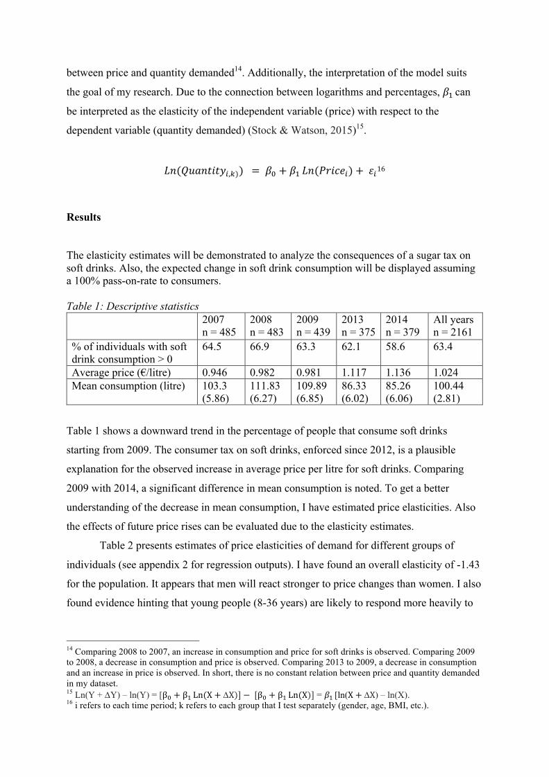
The elasticity estimates will be demonstrated to analyze the consequences of a sugar tax on soft drinks. Also, the expected change in soft drink consumption will be displayed assuming a 100% pass-on-rate to consumers. Table 1: Descriptive statistics 2007

n = 485 2008 n = 483

2009 n = 439

2013 n = 375

2014 n = 379

All years n = 2161

% of individuals with soft drink consumption > 0

64.5 66.9 63.3 62.1 58.6 63.4

Average price (€/litre) 0.946 0.982 0.981 1.117 1.136 1.024 Mean consumption (litre) 103.3

(5.86) 111.83 (6.27)

109.89 (6.85)

86.33 (6.02)

85.26 (6.06)

100.44 (2.81)

Table 1 shows a downward trend in the percentage of people that consume soft drinks

starting from 2009. The consumer tax on soft drinks, enforced since 2012, is a plausible

explanation for the observed increase in average price per litre for soft drinks. Comparing

2009 with 2014, a significant difference in mean consumption is noted. To get a better

understanding of the decrease in mean consumption, I have estimated price elasticities. Also

the effects of future price rises can be evaluated due to the elasticity estimates.

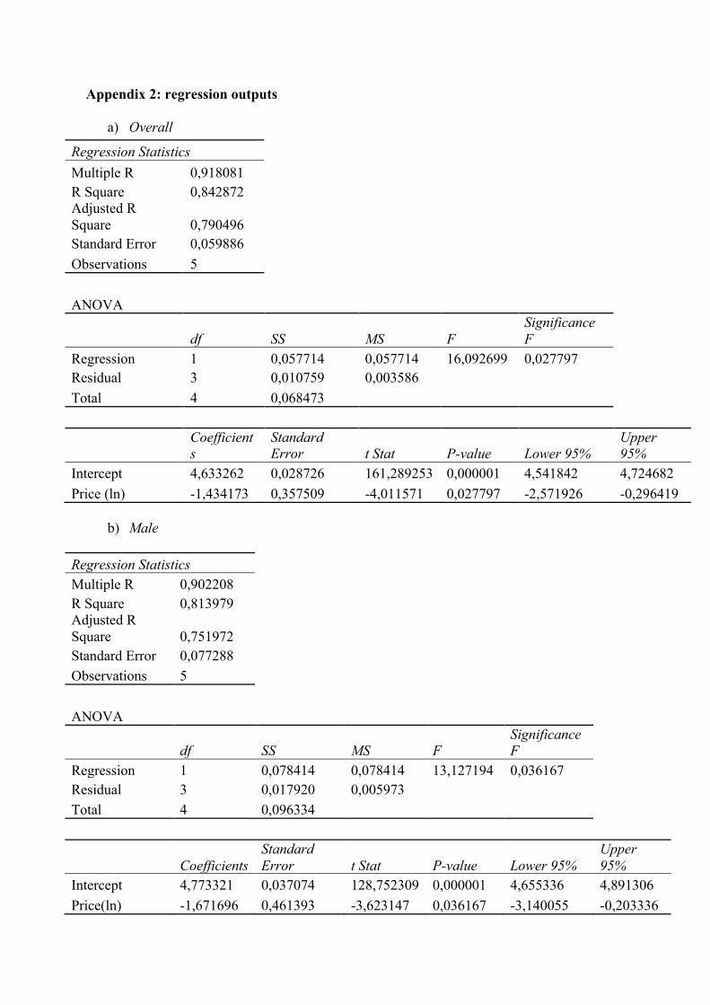
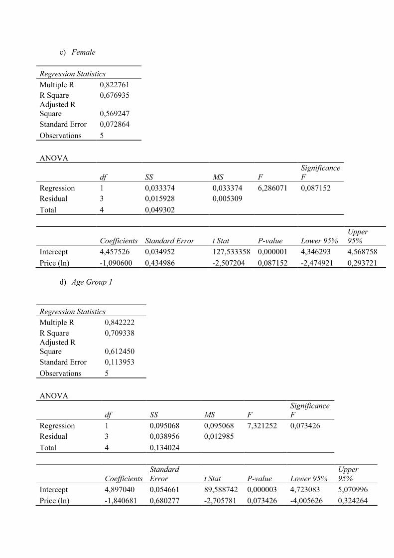
Table 2 presents estimates of price elasticities of demand for different groups of

individuals (see appendix 2 for regression outputs). I have found an overall elasticity of -1.43

for the population. It appears that men will react stronger to price changes than women. I also

found evidence hinting that young people (8-36 years) are likely to respond more heavily to

14 Comparing 2008 to 2007, an increase in consumption and price for soft drinks is observed. Comparing 2009 to 2008, a decrease in consumption and price is observed. Comparing 2013 to 2009, a decrease in consumption and an increase in price is observed. In short, there is no constant relation between price and quantity demanded in my dataset. 15 Ln(Y + DY) – ln(Y) = [β2 + β"Ln(X + DX)] − [β2 + β"Ln(X)] = 𝛽"[ln(X + DX) – ln(X). 16 i refers to each time period; k refers to each group that I test separately (gender, age, BMI, etc.).

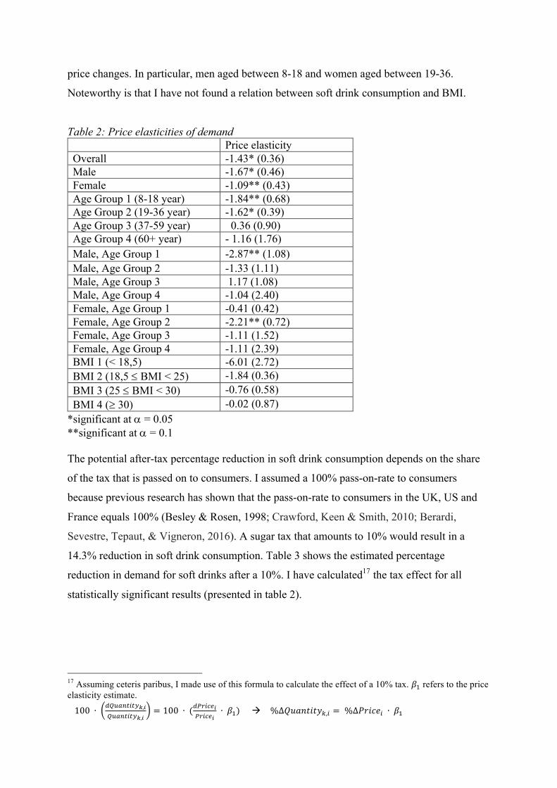
price changes. In particular, men aged between 8-18 and women aged between 19-36.

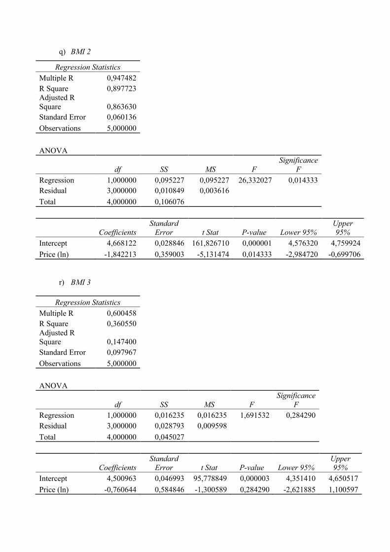
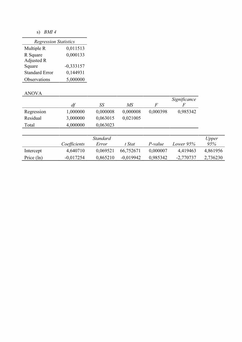
Noteworthy is that I have not found a relation between soft drink consumption and BMI.

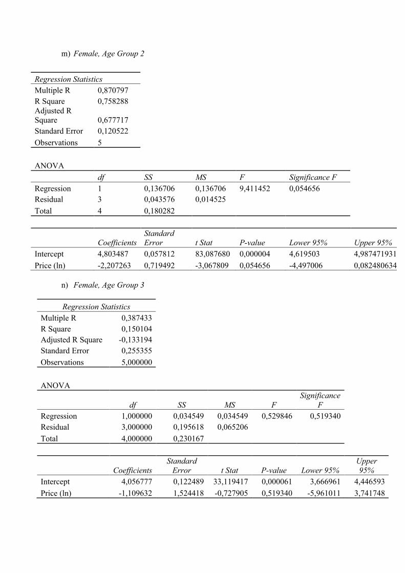
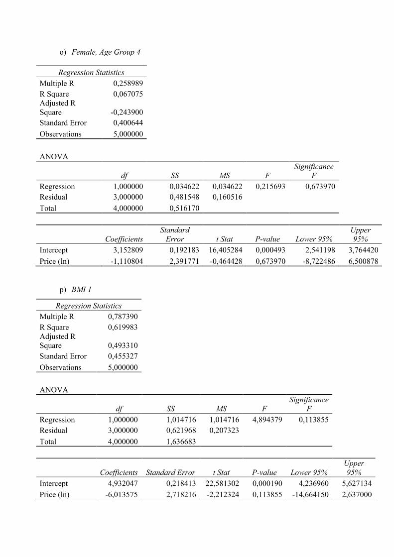
Table 2: Price elasticities of demand Price elasticity Overall -1.43* (0.36) Male -1.67* (0.46) Female -1.09** (0.43) Age Group 1 (8-18 year) -1.84** (0.68) Age Group 2 (19-36 year) -1.62* (0.39) Age Group 3 (37-59 year) 0.36 (0.90) Age Group 4 (60+ year) - 1.16 (1.76) Male, Age Group 1 -2.87** (1.08) Male, Age Group 2 -1.33 (1.11) Male, Age Group 3 1.17 (1.08) Male, Age Group 4 -1.04 (2.40) Female, Age Group 1 -0.41 (0.42) Female, Age Group 2 -2.21** (0.72) Female, Age Group 3 -1.11 (1.52) Female, Age Group 4 -1.11 (2.39) BMI 1 (< 18,5) -6.01 (2.72) BMI 2 (18,5 £ BMI < 25) -1.84 (0.36) BMI 3 (25 £ BMI < 30) -0.76 (0.58) BMI 4 (³ 30) -0.02 (0.87)

*significant at a = 0.05 **significant at a = 0.1 The potential after-tax percentage reduction in soft drink consumption depends on the share

of the tax that is passed on to consumers. I assumed a 100% pass-on-rate to consumers

because previous research has shown that the pass-on-rate to consumers in the UK, US and

France equals 100% (Besley & Rosen, 1998; Crawford, Keen & Smith, 2010; Berardi,

Sevestre, Tepaut, & Vigneron, 2016). A sugar tax that amounts to 10% would result in a

14.3% reduction in soft drink consumption. Table 3 shows the estimated percentage

reduction in demand for soft drinks after a 10%. I have calculated17 the tax effect for all

statistically significant results (presented in table 2).

17 Assuming ceteris paribus, I made use of this formula to calculate the effect of a 10% tax. 𝛽" refers to the price elasticity estimate.

100 ∙ DEFGHI-IJK,LEFGHI-IJK,L

= 100 ∙ (DMN-OPLMN-OPL

∙ 𝛽") à %∆𝑄𝑢𝑎𝑛𝑡𝑖𝑡𝑦/,- = %∆𝑃𝑟𝑖𝑐𝑒- ∙ 𝛽"

Table 3: Estimated % reduction in soft drink consumption after tax

t = 10% Overall 14.3 Male 16.7 Female 10.9 Age Group 1 18.4 Age Group 2 16.2 Male, Age Group 1 28.7 Female, Age Group 2 22.1

Conclusion

My price elasticity estimates infer that the demand for soft drinks is elastic. A tax of 10%,

assuming a pass-on-rate to consumers of 100%, results in a demand reduction of 14.3%.

People between 8-36 will be effected the most. More men than women are expected to

respond to price changes. No evidence for a correlation between BMI and the price

sensitivity for soft drinks has been found. All in all, a tax on soft drinks could be an effective

policy design if the goal is to reduce consumption among young people. Presuming that

obesity and heart diseases occur at an older age, a soft drink tax could lower future healthcare

costs and cause net benefits in the long run.

Discussion

I have estimated an overall price elasticity of -1.43 in the Netherlands. The biggest impact of

a sugar tax would be observed for teenage men (8-18) and young women (19-36). There is no

evidence to suggest that the effectiveness of a sugar tax differs across various BMI groups.

Based on my findings, middle-age and older people are not expected to react strongly to a

sugar tax. Consequently, my conclusions provide useful input into the current policy debate

on the merits of a tax on soft drinks. However, additional research on the effectiveness of a

sugar tax is required to formulate policy implications.

Strengths and limitations The strengths of my paper include the following. Foremost, it is the first study using the

National Dutch Food Consumption Survey of 2007-2010 and 2013-2014 to examine the

effect of a sugar tax on soft drinks. Previous research has been done for the Netherlands by

means of an experiment in a virtual supermarket (Waterlander et al., 2014), not by estimating

price elasticities. Secondly, it considers the effects of a tax for disparate groups, sorted by

gender, age and BMI.

My paper has several limitations. Due to limited availability of useful data, my

elasticity estimates are merely based on 5 inconsecutive time periods. Possibly, this results in

biased price elasticity estimates18. Ideally the sample size would be larger as well.

The empirical model that I have used to estimate price elasticities for demand is rather

simple. A more sophisticated model is likely to result in more reliable estimates, and thus

more useful results for policy makers.

Next, the way I had to estimate average soft drink price is quite cumbersome. As I

had to convert UK prices and currency, the precision of my average price estimate could be

weakened. I had to assume that the UK market is similar to the Dutch market in order to use

UK prices as a proxy for the Netherlands. In addition, I assumed the price level for soft

drinks to be similar to the one of non-alcoholic beverages.

I have only focused on own price elasticity. Cross-price elasticities should be

estimated for all substitute goods in order to oversee all consequences of a tax. If soft drinks

are replaced by other SSBs, taxation should be levied over these unhealthy substitutes as

well. Although my estimates add value to the existing knowledge regarding the effectiveness

of a sugar tax, it is crucial to know what individuals consume instead of soft drinks.

Policy implications My research is not sufficiently strong to result in policy implications. However, I have found

some useful results. My research shows strong indications regarding the value of a sugar tax.

I found out that in the Netherlands, there is no evidence to support the claim that a tax would

reduce consumption by obese people more than non-obese. On the other hand, it is expected

to affect young people who are the main consumers. This way it could be seen as an

instrument to limit the number of obese people in the future, and thus result in long-run

health benefits and healthcare cost savings.

To present a concrete tax proposal, further research is required to determine the type of tax

and to calculate the required level of taxation.

18 Due to unavailability of data, I could not include time periods 2010, 2011 and 2012 in my analysis. Therefore, my price elasticities can be overestimated, and thus biased.

Further research Many questions stay unanswered. Price elasticity estimates to influence public policy design

should be based on more time periods. On top of that, cross-price elasticity estimates are

required to understand the substitute effect.

I have calculated differential effects for gender, age and BMI groups. More factors

should be included in the estimation of elasticities. Counting for income level and urban

versus rural living conditions would add up to the applicability of elasticity estimates.

To test the effectiveness of a tax on soft drinks, multiple tax types should be tested.

Research in the US by Sharma, Hauck, Hollingsworth, & Siciliani (2014) has shown that a

flat tax on sales has distinct effects as compared to a volumetric tax. Moreover, the response

of soft drink manufacturers to a sugar tax is ambiguous. Taxing producers rather than

consumers is expected to have different results. Also, the tax pass-on-rate to consumers

should be computed to determine the real effects of a sugar tax.

Acknowledgement

I sincerely thank Andro Rilović for the supervision of my thesis. His comments have

significantly contributed to the quality of this research.

Also, my special thanks go to the RIVM for allowing me to use their dataset.

Bibliography

Alston, J. M., Foster, K. A., & Green, R. D. (1994). Estimating elasticities with the linear

approximate almost ideal demand system: some Monte Carlo results. The review of

Economics and Statistics, 351-356.

Andreyeva, T., Chaloupka, F. J., & Brownell, K. D. (2011). Estimating the potential of taxes

on sugar-sweetened beverages to reduce consumption and generate revenue. Preventive

medicine, 52(6), 413-416.

Berardi, N., Sevestre, P., Tepaut, M., & Vigneron, A. (2016). The impact of a ‘soda tax’ on

prices: evidence from French micro data. Applied Economics, 48(41), 3976-3994.

Besley, T. J., & Rosen, H. S. (1998). Sales taxes and prices: an empirical analysis (No.

w6667). National Bureau of Economic Research.

Briggs, A. D., Mytton, O. T., Madden, D., O’Shea, D., Rayner, M., & Scarborough, P.

(2013a). The potential impact on obesity of a 10% tax on sugar-sweetened beverages in

Ireland, an effect assessment modelling study. BMC Public Health, 13(1), 860.

Briggs, A. D., Mytton, O. T., Kehlbacher, A., Tiffin, R., Rayner, M., & Scarborough, P.

(2013b). Overall and income specific effect on prevalence of overweight and obesity of 20%

sugar sweetened drink tax in UK: econometric and comparative risk assessment modelling

study. Bmj, 347, f6189.

Briggs, A. (2016). Sugar tax could sweeten a market failure. Nature, 531(7596), 551-551.

Centers for disease control and prevention. (April 7, 2017). Get the Facts: Sugar-Sweetened

Beverages and Consumption. Retrieved from https://www.cdc.gov/nutrition/data-

statistics/sugar-sweetened-beverages-intake.html

Colchero, M. A., Salgado, J. C., Unar-Munguia, M., Hernandez-Avila, M., & Rivera-

Dommarco, J. A. (2015). Price elasticity of the demand for sugar sweetened beverages and

soft drinks in Mexico. Economics & Human Biology, 19, 129-137.

Crawford, I., Keen, M., & Smith, S. (2010). Value added tax and excises. Dimensions of tax

design: The Mirrlees review, 275-362.

Deaton, A., & Muellbauer, J. (1980). An almost ideal demand system. The American

economic review, 70(3), 312-326.

FWS. (2015). Kerngegevens 2015. Publication of the Dutch association for soft drinks,

waters and juices.

Green, R., & Alston, J. M. (1990). Elasticities in AIDS models. American Journal of

Agricultural Economics, 72(2), 442-445.

Guerrero-López, C. M., Unar-Munguía, M., & Colchero, M. A. (2017). Price elasticity of the

demand for soft drinks, other sugar-sweetened beverages and energy dense food in

Chile. BMC public health, 17(1), 180.

Hirschler, B. (2015, November 11). Diabetes experts tell G20 to tax sugar to save lives and

money. Reuters. Retrieved from http://www.reuters.com/article/us-health-diabetes-sugar-

idUSKCN0T100K20151112

International Diabetes Federation Europe. (2016). IDF Europe position on added sugar.

Malik, V. S., Schulze, M. B., & Hu, F. B. (2006). Intake of sugar-sweetened beverages and

weight gain: a systematic review. The American journal of clinical nutrition, 84(2), 274-288.

(n.d.). Sugar-sweetened beverages. Department of Health, State of Rhode Island. Retrieved

from http://www.health.ri.gov/healthrisks/sugarsweetenedbeverages/

Powell, L. M., & Chaloupka, F. J. (2009). Food prices and obesity: evidence and policy

implications for taxes and subsidies. Milbank Quarterly, 87(1), 229-257.

Sharma, A., Hauck, K., Hollingsworth, B., & Siciliani, L. (2014). The effects of taxing sugar-

sweetened beverages across different income groups. Health economics, 23(9), 1159-1184.

Stock, J.H. and Watson, M.W. (2015). Introduction to Econometrics (updated third edition

(global edition)). Essex: Pearson Education.

Statista. (2017). Average price of soft drinks in the United Kingdom (UK) from 2008 to 2015

(in GBP per litre). Retrieved from https://www.statista.com/statistics/308926/average-soft-

drink-price-in-the-united-kingdom-uk/

Vartanian, L. R., Schwartz, M. B., & Brownell, K. D. (2007). Effects of soft drink

consumption on nutrition and health: a systematic review and meta-analysis. American

journal of public health, 97(4), 667-675.

Waterlander, W. E., Steenhuis, I. H., de Boer, M. R., Schuit, A. J., & Seidell, J. C. (2012).

Introducing taxes, subsidies or both: the effects of various food pricing strategies in a web-

based supermarket randomized trial. Preventive Medicine, 54(5), 323-330.

Waterlander, Wilma Elzeline, Cliona Ni Mhurchu, and Ingrid HM Steenhuis. "Effects of a

price increase on purchases of sugar sweetened beverages. Results from a randomized

controlled trial." Appetite 78 (2014): 32-39.

World Health Organization. (2015). Fiscal policies for diet and prevention of

noncommunicable diseases. Geneva, Switzerland.

Zizzo, D. J., Parravano, M., Nakamura, R., Forwood, S., & Suhrcke, M. (2016). The impact

of taxation and signposting on diet: an online field study with breakfast cereals and soft

drinks (No. 131cherp).

Appendix 1: Age groups & BMI groups

Age groups:

Age Group 1 8-18 year



Age Group 4 60+ year

BMI groups:

BMI Group 1 < 18,5 Underweight

BMI Group 2 18,5 £ BMI < 25 Normal weight

BMI Group 3 25 £ BMI < 30 Overweight

BMI Group 4 BMI ³ 30 Obesity

Appendix 2: regression outputs

a) Overall

b) Male

Regression Statistics Multiple R 0,902208 R Square 0,813979 Adjusted R Square 0,751972 Standard Error 0,077288 Observations 5 ANOVA

df SS MS F Significance F

Regression 1 0,078414 0,078414 13,127194 0,036167 Residual 3 0,017920 0,005973 Total 4 0,096334

Coefficients Standard Error t Stat P-value Lower 95%

Upper 95%

Intercept 4,773321 0,037074 128,752309 0,000001 4,655336 4,891306 Price(ln) -1,671696 0,461393 -3,623147 0,036167 -3,140055 -0,203336




Coefficients

Standard Error t Stat P-value Lower 95%

Upper 95%

Intercept 4,633262 0,028726 161,289253 0,000001 4,541842 4,724682 Price (ln) -1,434173 0,357509 -4,011571 0,027797 -2,571926 -0,296419

c) Female




Coefficients Standard Error t Stat P-value Lower 95% Upper 95%

Intercept 4,457526 0,034952 127,533358 0,000001 4,346293 4,568758 Price (ln) -1,090600 0,434986 -2,507204 0,087152 -2,474921 0,293721

d) Age Group 1





Upper 95%


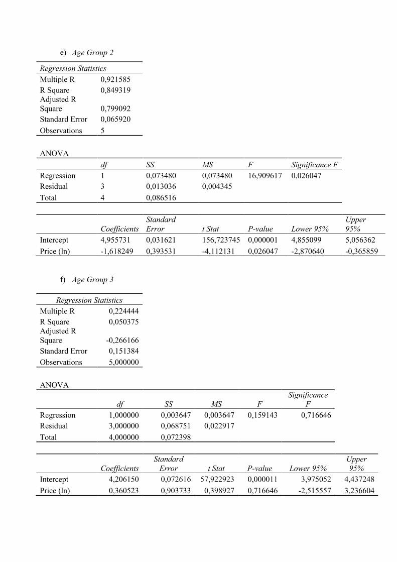
e) Age Group 2

f) Age Group 3

Regression Statistics Multiple R 0,224444 R Square 0,050375 Adjusted R Square -0,266166 Standard Error 0,151384 Observations 5,000000 ANOVA

df SS MS F Significance

F Regression 1,000000 0,003647 0,003647 0,159143 0,716646 Residual 3,000000 0,068751 0,022917 Total 4,000000 0,072398

Coefficients Standard

Error t Stat P-value Lower 95% Upper 95%

Intercept 4,206150 0,072616 57,922923 0,000011 3,975052 4,437248 Price (ln) 0,360523 0,903733 0,398927 0,716646 -2,515557 3,236604

Regression Statistics Multiple R 0,921585 R Square 0,849319 Adjusted R Square 0,799092 Standard Error 0,065920 Observations 5 ANOVA df SS MS F Significance F Regression 1 0,073480 0,073480 16,909617 0,026047 Residual 3 0,013036 0,004345 Total 4 0,086516


Upper 95%


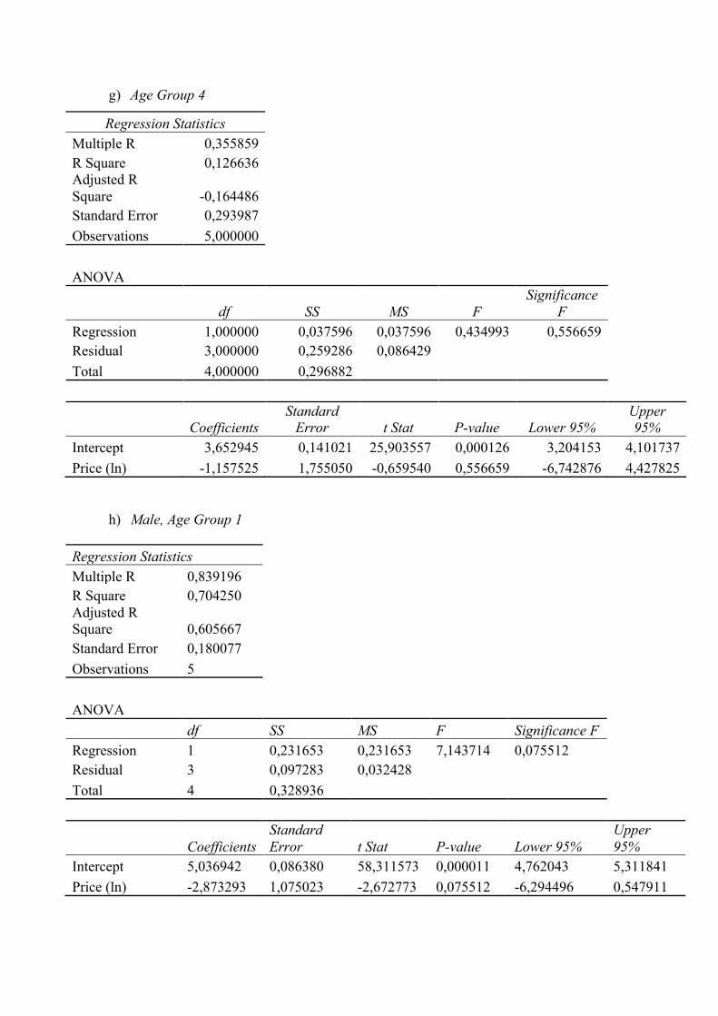
g) Age Group 4

h) Male, Age Group 1



Upper 95%








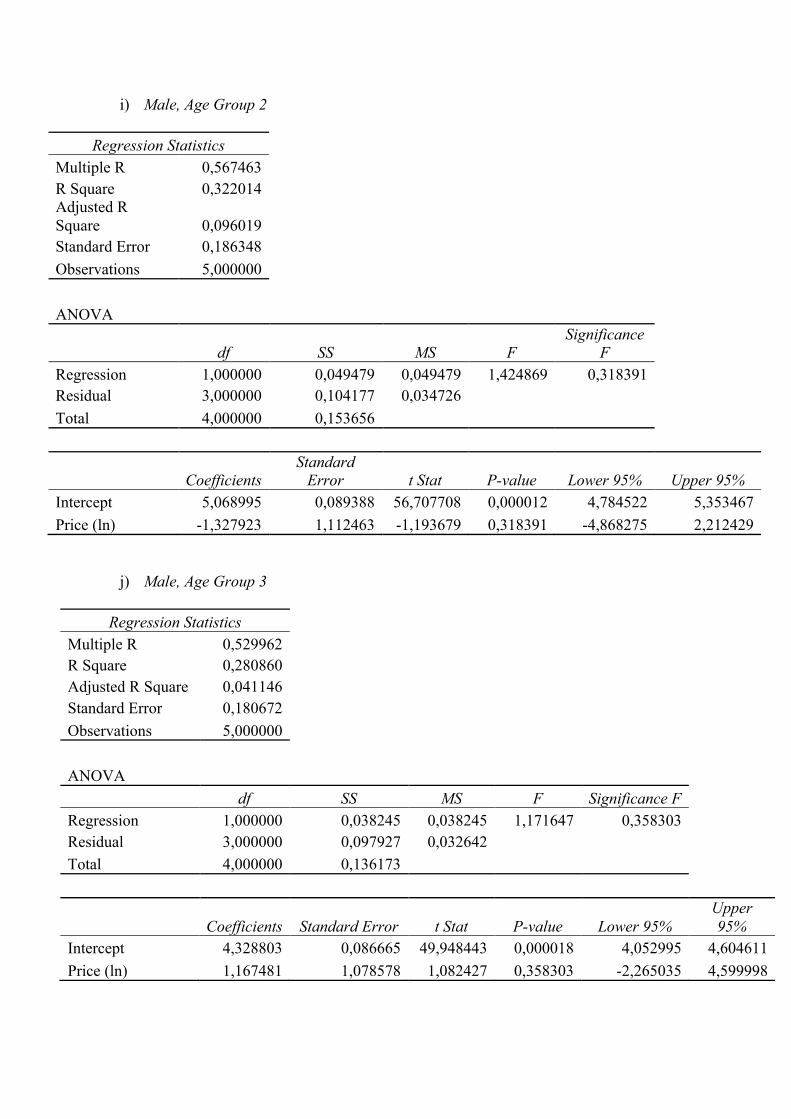
i) Male, Age Group 2 Regression Statistics

Multiple R 0,567463 R Square 0,322014 Adjusted R Square 0,096019 Standard Error 0,186348 Observations 5,000000 ANOVA




Error t Stat P-value Lower 95% Upper 95% Intercept 5,068995 0,089388 56,707708 0,000012 4,784522 5,353467 Price (ln) -1,327923 1,112463 -1,193679 0,318391 -4,868275 2,212429

j) Male, Age Group 3

Regression Statistics Multiple R 0,529962 R Square 0,280860 Adjusted R Square 0,041146 Standard Error 0,180672 Observations 5,000000 ANOVA

df SS MS F Significance F Regression 1,000000 0,038245 0,038245 1,171647 0,358303 Residual 3,000000 0,097927 0,032642 Total 4,000000 0,136173


Intercept 4,328803 0,086665 49,948443 0,000018 4,052995 4,604611 Price (ln) 1,167481 1,078578 1,082427 0,358303 -2,265035 4,599998

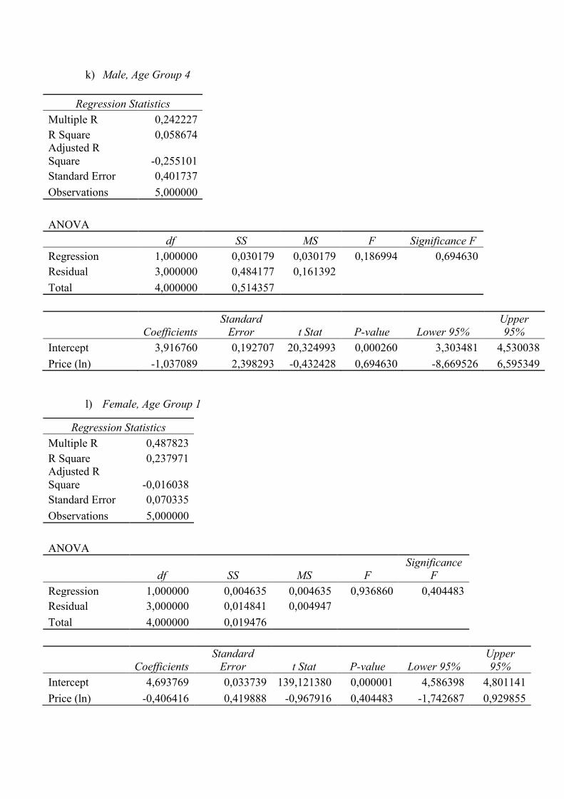
k) Male, Age Group 4


df SS MS F Significance F Regression 1,000000 0,030179 0,030179 0,186994 0,694630 Residual 3,000000 0,484177 0,161392 Total 4,000000 0,514357




l) Female, Age Group 1







m) Female, Age Group 2

n) Female, Age Group 3

Regression Statistics

Multiple R 0,387433 R Square 0,150104 Adjusted R Square -0,133194 Standard Error 0,255355 Observations 5,000000 ANOVA









o) Female, Age Group 4







p) BMI 1






q) BMI 2

r) BMI 3













s) BMI 4







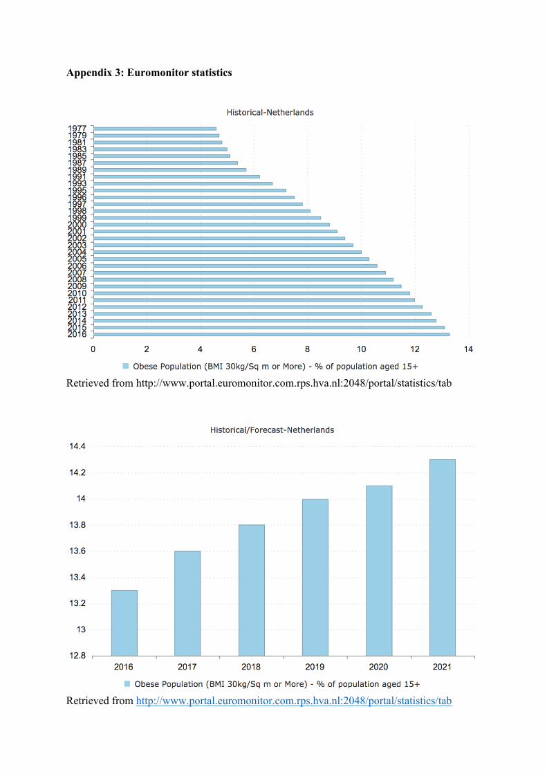
Appendix 3: Euromonitor statistics

Retrieved from http://www.portal.euromonitor.com.rps.hva.nl:2048/portal/statistics/tab

Retrieved from http://www.portal.euromonitor.com.rps.hva.nl:2048/portal/statistics/tab

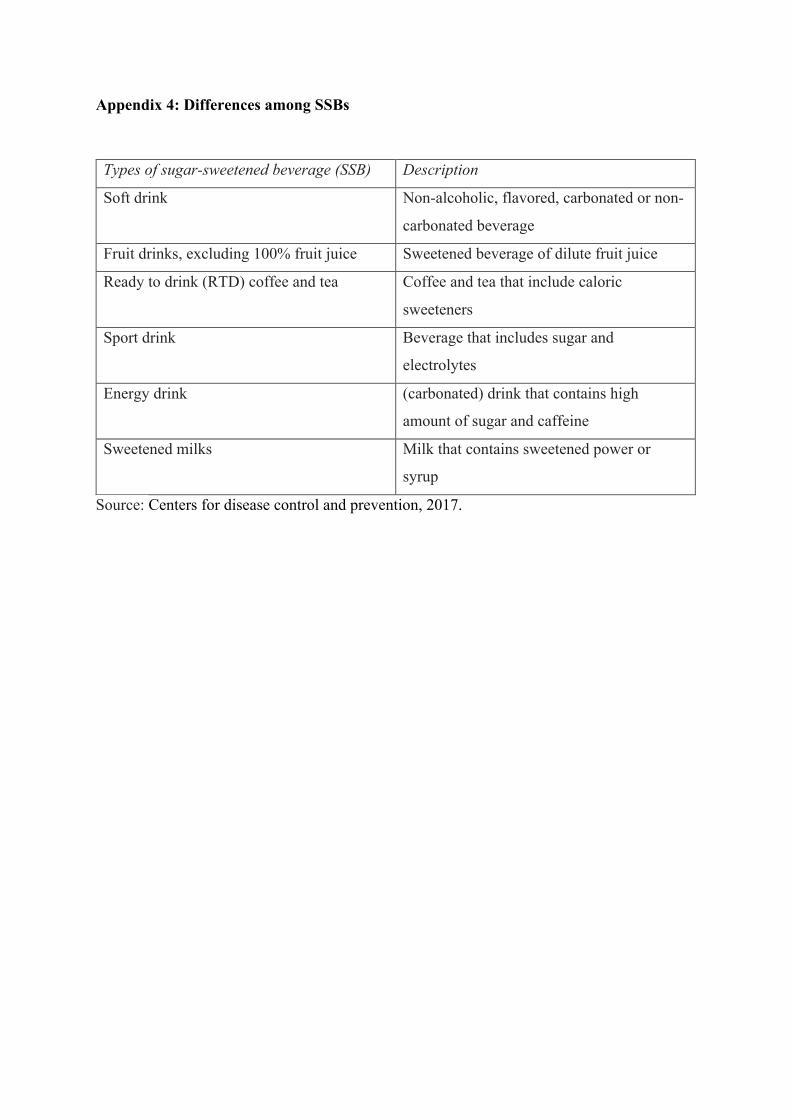
Appendix 4: Differences among SSBs

Types of sugar-sweetened beverage (SSB) Description

Soft drink Non-alcoholic, flavored, carbonated or non-

carbonated beverage

Fruit drinks, excluding 100% fruit juice Sweetened beverage of dilute fruit juice

Ready to drink (RTD) coffee and tea Coffee and tea that include caloric

sweeteners

Sport drink Beverage that includes sugar and

electrolytes

Energy drink (carbonated) drink that contains high

amount of sugar and caffeine

Sweetened milks Milk that contains sweetened power or

syrup

Source: Centers for disease control and prevention, 2017.

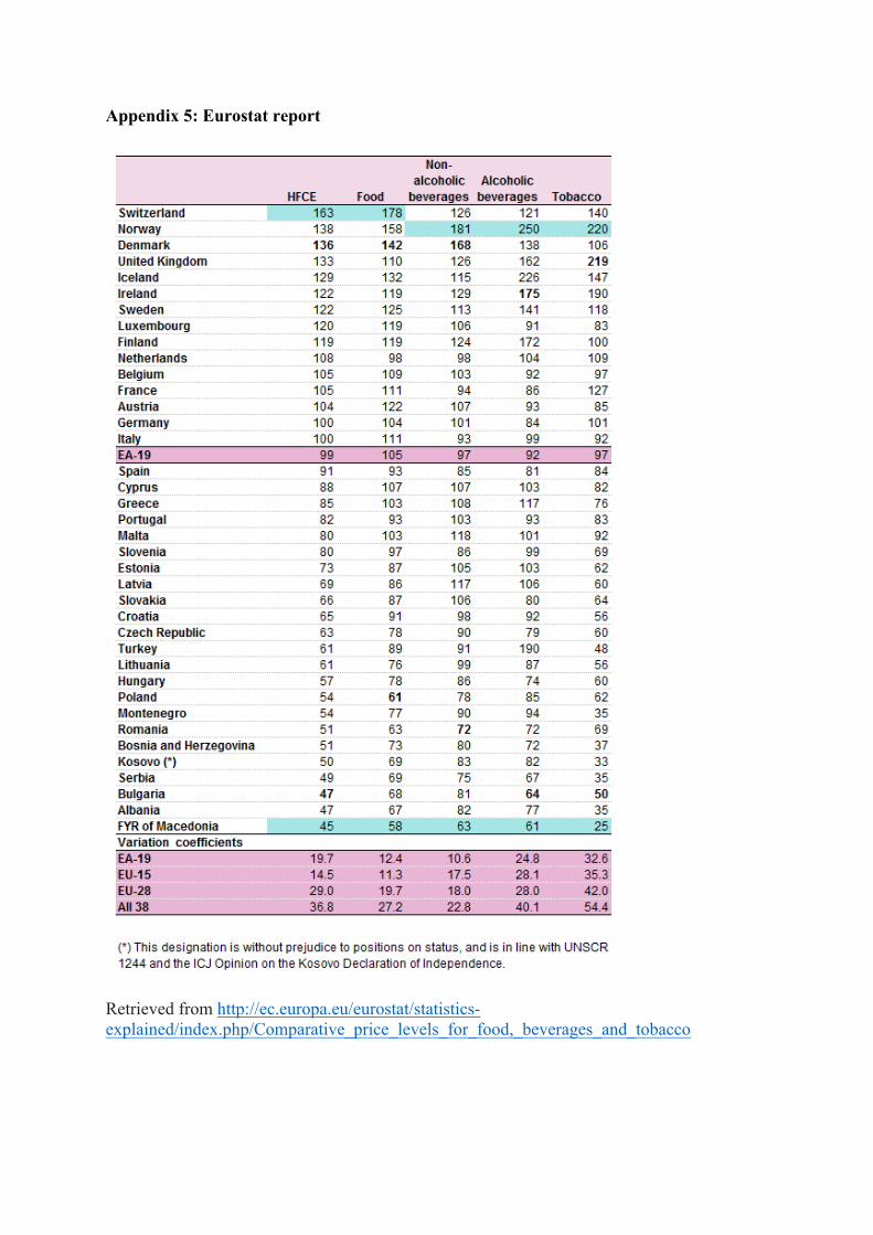
Appendix 5: Eurostat report

Retrieved from http://ec.europa.eu/eurostat/statistics-explained/index.php/Comparative_price_levels_for_food,_beverages_and_tobacco

Price elasticity of the demand for soft drinks in the Netherlands ...

Documents

Transcript of Price elasticity of the demand for soft drinks in the Netherlands ...