TESLA Report 2003-21

Cavity Control System – Optimization Methods For Single Cavity Driving and Envelope Detection.

Tomasz Czarski, Ryszard Romaniuk, Krzysztof Poźniak

ELHEP Laboratory, ISE, Warsaw University of Technology Stefan Simrock

TESLA, DESY, Hamburg

ABSTRACT The paper is an introduction to the optimization methods of the linear accelerator cavity control system. Three distinct time periods of cavity operation are considered; filling with the EM field energy, field stabilization for the accelerated beam, and field decay. These periods are considered as different states of the cavity corresponding to adequate solutions of differential equation modeling the cavity behavior. The cavity could be operated by several different methods in each work phase: During the filling – feedback and feed-forward alone, feedback and feed-forward together, self-tuning; During the flattop – feed-forward and feedback alone or together, During the decay – detuning and quality factor may be measured. The optimization is understood as a choice of the most efficient way of the cavity control during each period. The control may be done in terms of minimum power consumption from the klystron during whole work cycle and efficient field stabilization in the cavity, during flattop period. The introductory analysis of the cavity operational modes in three mentioned periods is presented in this paper. Additionally, the alternative, more precise algorithm of the cavity field detection is proposed. The cavity field is estimated as a result of intermediate frequency signal envelope decoding. All considerations in this paper deal with a single cavity system in noiseless and deterministic conditions.

Keywords: Superconducting cavity control, linear accelerators, control theory, free electron laser

1. INTRODUCTION

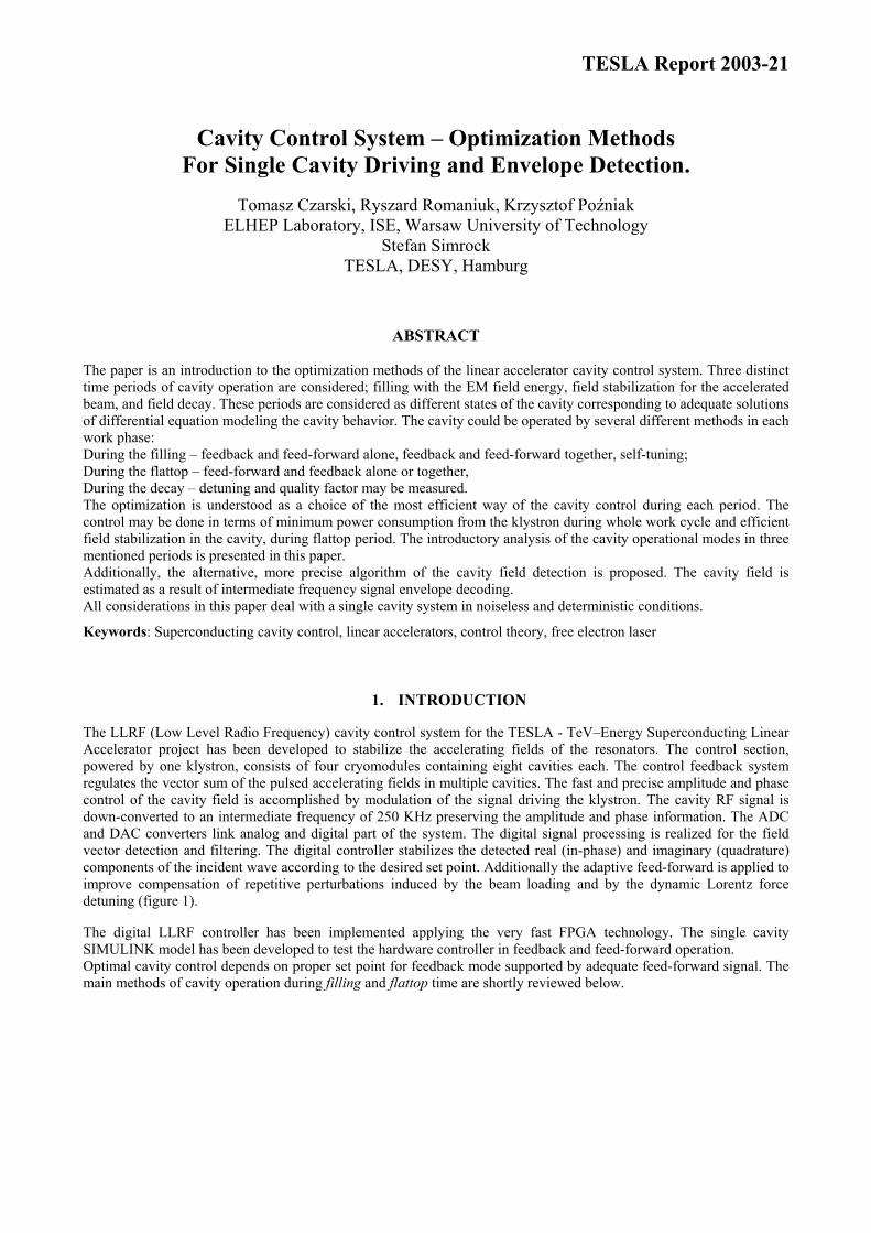
The LLRF (Low Level Radio Frequency) cavity control system for the TESLA - TeV–Energy Superconducting Linear Accelerator project has been developed to stabilize the accelerating fields of the resonators. The control section, powered by one klystron, consists of four cryomodules containing eight cavities each. The control feedback system regulates the vector sum of the pulsed accelerating fields in multiple cavities. The fast and precise amplitude and phase control of the cavity field is accomplished by modulation of the signal driving the klystron. The cavity RF signal is down-converted to an intermediate frequency of 250 KHz preserving the amplitude and phase information. The ADC and DAC converters link analog and digital part of the system. The digital signal processing is realized for the field vector detection and filtering. The digital controller stabilizes the detected real (in-phase) and imaginary (quadrature) components of the incident wave according to the desired set point. Additionally the adaptive feed-forward is applied to improve compensation of repetitive perturbations induced by the beam loading and by the dynamic Lorentz force detuning (figure 1).

The digital LLRF controller has been implemented applying the very fast FPGA technology. The single cavity SIMULINK model has been developed to test the hardware controller in feedback and feed-forward operation. Optimal cavity control depends on proper set point for feedback mode supported by adequate feed-forward signal. The main methods of cavity operation during filling and flattop time are shortly reviewed below.

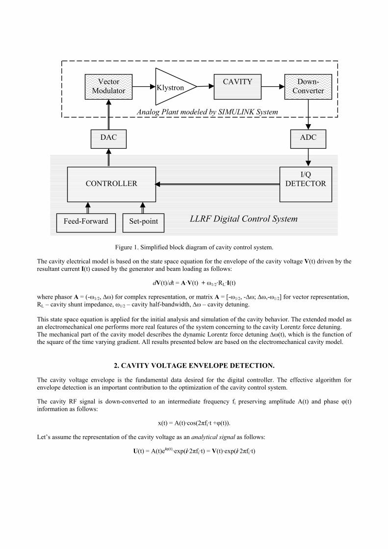
Analog Plant modeled by SIMULINK System

DAC ADC

LLRF Digital Control System Set-point Feed-Forward

Klystron

CONTROLLER

I/Q DETECTOR

Vector Modulator

Down- Converter

CAVITY

Figure 1. Simplified block diagram of cavity control system.

The cavity electrical model is based on the state space equation for the envelope of the cavity voltage V(t) driven by the resultant current I(t) caused by the generator and beam loading as follows:

dV(t)/dt = A·V(t) + ω1/2·RL·I(t)

where phasor A = (-ω1/2, ∆ω) for complex representation, or matrix A = [-ω1/2, -∆ω; ∆ω,-ω1/2] for vector representation, RL – cavity shunt impedance, ω1/2 – cavity half-bandwidth, ∆ω – cavity detuning. This state space equation is applied for the initial analysis and simulation of the cavity behavior. The extended model as an electromechanical one performs more real features of the system concerning to the cavity Lorentz force detuning. The mechanical part of the cavity model describes the dynamic Lorentz force detuning ∆ω(t), which is the function of the square of the time varying gradient. All results presented below are based on the electromechanical cavity model.

2. CAVITY VOLTAGE ENVELOPE DETECTION.

The cavity voltage envelope is the fundamental data desired for the digital controller. The effective algorithm for envelope detection is an important contribution to the optimization of the cavity control system.

The cavity RF signal is down-converted to an intermediate frequency fi preserving amplitude A(t) and phase φ(t) information as follows:

x(t) = A(t)·cos(2πfi·t +φ(t)).

Let’s assume the representation of the cavity voltage as an analytical signal as follows:

U(t) = A(t)eiφ(t)·exp(i·2πfi·t) = V(t)·exp(i·2πfi·t)

where the complex envelope V(t) = A(t)eiφ(t) with the real part called in-phase component (I), and the imaginary part called quadrature component (Q).

The digital signal processing is performed applying the signal of intermediate frequency as a real part of an analytical signal with sampling period T =1/4fi.

Therefore the analytical signal U(t) = U(kT) = Uk for successive samples k is as follows

Uk = V(kT)·exp(i·2πfi·kT) = Vk·(i)k = xk + i·yk

where sample of the real signal equals xk and the imaginary sample equals yk.

Zero Order Envelope Detection.

Let’s assume the stable value of an amplitude and phase of the cavity voltage for successive steps k, so that Vk-1 = Vk = const.

Two consecutive samples of the real signal xk-1, xk are required for zero order envelope detection according to relations:

Vk-1·(i)k-1 = xk-1 + i·yk-1 and Vk·(i)k = xk + i·yk.

Applying upper equations the complex envelope is determined by digital demodulation as follows:

Vk = (xk + i·yk-1)(-i)k

First Order Envelope Detection.

More accurate estimation of (I, Q) components is required for fast varying envelope during cavity filling time.

Let’s assume linearly time varying complex envelope for successive steps k with mutual difference of ∆V, as follows:

Vk-1 = Vk - ∆V, Vk+1 = Vk + ∆V.

Three sequential samples of the real signal xk-1, xk, xk+1 are required for first order envelope detection according to the relations:

(Vk - ∆V)·(i)k-1 = xk-1 + i·yk-1 Vk·(i)k = xk + i·yk (Vk + ∆V)·(i)k+1 = xk+1 + i·yk+1.

Applying upper equations the complex envelope is determined by digital demodulation as follows:

Vk = (xk + i·(xk-1 – xk+1)/2)·(-i)k .

The first order envelope detection algorithm may possibly engage more samples covering the period of the intermediate frequency signal for an advance improvement.

Five sequential samples of the real signal xk-2, xk-1, xk, xk+1 xk+2, are required for modified algorithm of the first order envelope detection, removing the offset of the intermediate frequency signal according to the relations:

Vk = (Vk-1 + Vk+1 )/2 = ((xk – xk-2)/4 + (xk – xk+2)/4 + i·(xk-1 – xk+1)/2)·(-i)k .

Therefore the averaging process is involved causing better envelope estimation and efficient offset removing for intermediate frequency signal.

Furthermore the fitting calibration factor corrects the resultant cavity voltage envelope and compensates the measurement channel attenuation and phase shifting for an individual cavity.

Both algorithms for the cavity voltage envelope detection are implemented in the MATLAB controller coupled to the SIMULINK cavity. The simulation results are presented in figure 2 and comparisons of errors are presented in figure 3. The results for the real off-line signal envelope detection are presented in figure 4 for both algorithms.

Figure 2. SIMULINK cavity output and MATLAB output for I/Q detector and controller in feedback operation.

Two envelope algorithms are applied for different periods of cavity filling time.

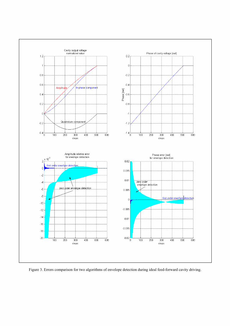
Figure 3. Errors comparison for two algorithms of envelope detection during ideal feed-forward cavity driving.

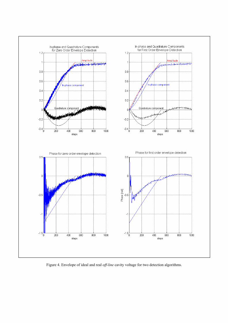
Figure 4. Envelope of ideal and real off-line cavity voltage for two detection algorithms.

3. CAVITY FILLING OPERATION

The main purpose of the cavity filling is to achieve proper operating conditions for the beam loading. The cavity is filled with the preset, constant, forward power, during the first stage of operation. This results in an exponential increase of the envelope of RF electromagnetic field according to its natural behavior in the resonance condition. But the Lorentz force decreases the cavity resonance frequency with the rising field gradient.

Lets assume a phase modulated current step as an envelope of cavity input, in the complex domain of (I, Q)

I(t) = Io·exp(iΦ(t))

The appropriate phase modulation Φ(t) of the incident wave compensates the time varying cavity detuning ∆ω(t), if

dΦ/dt = ∆ω(t).

Thus, the RF signal follows the cavity resonance frequency.

The envelope of the cavity response in the complex domain of (I, Q), as a solution of the state space equation, is as follows:

V(t) = Io·RL·(1– exp(-ω1/2·t))·exp(iΦ(t)),

where, ω1/2 = cavity half-bandwidth and RL = cavity load resistance.

Therefore, the exponential relation between the cavity input, with stable magnitude, and the cavity output is valid in the resonance condition, as follows:

V(t)/I(t) = RL·(1– exp(-ω1/2·t))

Thus, the zero input-output phase difference is enforced.

The required phase Φ(t) is the integral of the detuning, for the given function ∆ω(t). The amplitude of the cavity voltage attains half of the asymptotic value (for ideal case) at the beam injection instant Tf = ln2/ω1/2, and is set stable as the desired value |V| at the flattop level. The proper initial condition Φ0 = Φ(0) adjusts the required final flattop value Φ(Tf) = φ for filling time Tf.

Thus, the cavity can be driven in the resonance condition during the filling time, for the given cavity detuning ∆ω(t):

- in feed-forward mode by the proper phase modulated step of the incident wave:

i(t) = 2|V|·exp(iΦ(t))/RL

- in feedback mode by the phase modulated exponentially rising set-point:

v(t) = 2|V|·(1– exp(-ω1/2·t))·exp(iΦ(t)).

On the other hand, the cavity can drive itself in the resonance without external detuning information in so-called self-tuning mode. It is a kind of a self-exciting mode, where the controller forces the cavity input initial condition. The cavity is driven by constant current equal Io = 2|V|·exp(iΦ0)/RL during the initial step corresponding to the sampling period T. The resultant cavity output ∆V can be estimated as ∆V/|V| ≈ 2ω1/2·T relatively to the final value |V| desired at the flattop level. The cavity output takes driving itself, for any step number k≥1, according to the resonance relation:

I(k·T) = V(k·T)/(RL·(1– exp(-ω1/2·k·T))). Therefore, the cavity forces itself to track its resonance frequency. The digital controller applies the table with exponentially changing values and equalizes the cavity output and input phases.

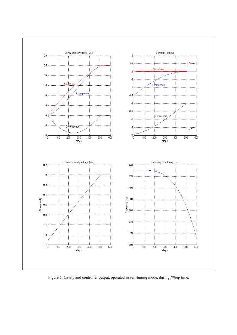
Figure 5. Cavity and controller output, operated in self-tuning mode, during filling time.

In any case, the magnitude of the current |Io| = 2|V|/RL and the initial phase Φ0 should be correctly established, so that to accomplish the desired steady state at the flattop level.

The cavity control system has been modeled applying the Matlab code. Three modes of the cavity filling operation have been implemented for sampling time T=1µs. The auto calibration algorithm has been developed for initial phase Φ0, from pulse to pulse, in the Matlab system. The simulation results for the self-tuning mode of the cavity operation, for the Matlab system, are presented in figure 5. The results agree with the feed-forward operation for the given cavity detuning ∆ω(t) during filling time.

4. CAVITY FLATTOP OPERATION

The envelope of the cavity voltage is stable during the flattop operation at the expense of an additional power reflected, due to the mismatch caused by the cavity detuning. The solution of the state space equation, for the steady state, in complex domain of (I, Q), is as follows:

V = I·RL/(1-i∆ω/ω1/2) = I·RLcos ψ·eiψ

where, voltage phasor V - desired envelope of the cavity output value, resultant current phasor I - required envelope of the cavity input value and tuning angle ψ = tan-1(∆ω/ω1/2).

The driving feed-forward current If can be estimated, for the stable value V=|V|eiφ desired at the flattop level, with the beam loading Ib, and the detuned cavity, as follows:

If = |V|eiφ·(1– i∆ω/ω1/2)/RL + Ib, where If - Ib = I.

Thus, the predicted current component, equal to Ib, compensates the beam loading current, and detuning dependent factor ∆ω/ω1/2, compensates the cavity impedance variation. The required input current can be established, for the given cavity detuning ∆ω(t), and results in the desired cavity output. The simulation results of the feed-forward operation for the Matlab system are presented in figure 6. The required cavity voltage can be as well accomplished through the feedback operation with accuracy limited by the controller gain with set-point value V=|V|eiφ without cavity detuning information.

The simulation results of feedback operation are presented in figure 7 for the Matlab system.

To minimize the peak power the proper cavity pre-detuning ∆ω0 shifts the time varying detuning, so that required forward power is symmetrically extended along the flattop range. The cavity pre-detuning ∆ω0 and initial phase Φ0 are adequately set up for all changes of the cavity operating parameters. On the other hand, the results achieved by the feedback mode, carry information about the condition of the cavity operation during one pulse. The controller output for feedback mode is approximated reproduction of the ideal feed-forward signal (compare figure 6 and 7). Therefore, the cavity detuning during the pulse can be estimated applying (I, Q) relation for the steady state as follows:

∆ω(t) ≈ -ω1/2·RL/|V|·Im(I·e-iφ),

The result of detuning estimation compare to the cavity model detuning monitoring for feedback mode is presented in figure 7.

Figure 6. Cavity and controller output, operated by ideal feed-forward, during filling and flattop time.

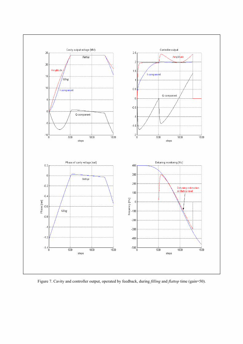
Figure 7. Cavity and controller output, operated by feedback, during filling and flattop time (gain=50).

5. CAVITY DECAY OPERATION

The envelope of the cavity voltage yields an exponential decay, after turning off both the generator and the beam, according to the homogeneous solution of the state space equation in complex domain of (I, Q) as follows:

V(t) = |V|eiφ·exp(-ω1/2+i∆ω)t = v(t)·exp(-iΦ(t)).

where, time dependent amplitude v(t) = |V|·exp(-ω1/2·t), and phase Φ(t) = ∆ω·t + φ. Therefore, the cavity parameters can be determined according to the equations, in turning off instant:

cavity half-bandwidth ω1/2 = – dv/dt /v(t)

cavity detuning ∆ω = dΦ/dt

6. CONCLUSIONS The algorithm of the first order envelope detection has been verified as much better estimation of (I, Q) components comparing to zero order one for fast varying envelope during cavity filling time. The comprehensive reduction of the systematic error (offset) is the substantial feature of that algorithm.

The efficient feedback or feed-forward mode can be applied only on condition that we possess information about the time varying cavity detuning during filling time. Thus, the self-tuning method is the only solution for optimal cavity driving during filling time requiring no information of the cavity detuning.

The efficient flattop feed-forward mode can be applied only on condition that we possess information about the time varying cavity detuning. The desired cavity voltage can be accomplished through the flattop feedback operation with accuracy limited by the controller gain without cavity detuning information. The results achieved by the feedback mode, provide some information about the cavity operation during one pulse. For example time varying cavity detuning can be estimated. It is to consider how to apply this information for successive pulses in repetitive conditions.

The feedback/feed-forward and self-tuning methods seem at first sight apparently exclusive. It turns out, however, that in real conditions, they may be efficiently supplemented. This results in a comparatively new method of weighted cavity control incurring the usage of self-tuning and feedback/feed-forward methods together.

REFERENCES

1. T.Czarski, R.Romaniuk, K.Poźniak, S.Simrock, TESLA Technical Note, 2003-06,

http://tesla.desy.de/new_pages/TESLA/TTFnot03.html