applied sciences

Article

Grounding Electrodes with Internal Resistance: Application toFeasibility Study of the Driven-Rod Method for Modeling theSoil Electrical Resistivity Profile

Gregorio Denche, Eduardo Faleiro * , Gabriel Asensio and Jorge Moreno

Citation: Denche, G.; Faleiro, E.;

Asensio, G.; Moreno, J. Grounding

Electrodes with Internal Resistance:

Application to Feasibility Study of the

Driven-Rod Method for Modeling the

Soil Electrical Resistivity Profile. Appl.

Sci. 2021, 11, 5032. https://doi.org/

10.3390/app11115032

Received: 12 May 2021

Accepted: 26 May 2021

Published: 29 May 2021

Publisher’s Note: MDPI stays neutral

with regard to jurisdictional claims in

published maps and institutional affil-

iations.

Copyright: © 2021 by the authors.

Licensee MDPI, Basel, Switzerland.

This article is an open access article

distributed under the terms and

conditions of the Creative Commons

Attribution (CC BY) license (https://

creativecommons.org/licenses/by/

4.0/).

Escuela Técnica Superior de Ingeniería y Diseño Industrial, Universidad Politécnica de Madrid,28012 Madrid, Spain; gregorio.denche@upm.es (G.D.); gabriel.asensio@upm.es (G.A.);jorge.moreno@upm.es (J.M.)* Correspondence: eduardo.faleiro@upm.es

Featured Application: The model proposed in the paper can be applied to any electrode to assessthe impact of its internal resistance on the main parameters that define a grounding system.

Abstract: The paper presents a model to include the internal resistance of the grounding electrodesin the calculation of its electrical features. The semi-analytical expressions for the calculation ofthe grounding resistance arising from the model are used to study the feasibility of the driven-rodmethod for the estimation of the soil resistivity profile since, unlike other methods, the internalresistance of the conductors can be of great influence for a correct estimate. From the groundingresistance profile an inverse problem based on the minimization of the quadratic differences betweenthe resistance measured and that calculated from the model is posed. Several synthetic examplesare used to assess the limitations of the method in conditions close to real situations. Finally, somereal cases involving data measured in the field are analyzed. Whether in synthetic examples or inreal soils it is found that the spatial frequency of the driven-rod resistance sampling is a determinantfactor in order to study the feasibility of the driven–rod method.

Keywords: non-zero internal resistance electrode; driven-rod method; grounding resistance logging;soil parameters optimization

1. Introduction

The estimation of the soil resistivity as a function of the depth is a key point for modellingany grounding system [1]. There are several methods to determine the soil resistivity. Most ofthem are indirect methods that use an intermediate magnitude as the apparent resistivity. Inone of the most used methods, the resistivity is estimated from a vertical electrical sounding(VES) performed with a four-pin device as in the Wenner and Schlumberger arrays, fromwhich the apparent resistivity is obtained [2]. From the apparent resistivity, it is possible tofind out the soil resistivity profile, provided that a constant multi-layered model has beenadopted [3,4]. Even though the VES is a non-invasive procedure, small errors in the measuringprocedure could lead to a soil model far from the real one. The ill-conditioned nature of themethod to obtain the resistivity profile from the soil’s apparent resistivity is at the bottomof the issue [5,6]. On the other hand, in some sense a VES could be seen as a non-local testsince the soil conductivity between the active electrodes of the test array is being checked.Note for instance that in a Wenner array the active electrodes are separated three times thedistance between adjacent probes. The soil properties could change horizontally leading to asoil resistivity profile that would not match with the real one. This is especially importantwhen a grounding system makes use of vertical rods as grounding electrodes, such as in thecase of lightning protection electrodes.

Another indirect procedure sometimes used is the driven-rod method. In this method,the grounding resistance of a rod driven into the ground is measured by the fall-of-potential

Appl. Sci. 2021, 11, 5032. https://doi.org/10.3390/app11115032 https://www.mdpi.com/journal/applsci

Appl. Sci. 2021, 11, 5032 2 of 16

procedure [7]. If the rod is modeled as a cylinder of length L and radius r, where L >> rand with a hemisphere at the end, the grounding resistance in a homogeneous mediumof resistivity, rho, is R = ρ

2πL ln( 2Ld ). On the other hand, if the rod is modeled as a half-

ellipsoid of revolution, whose major axis is L and its minor axis is the diameter d, theexpression R = ρ

2πL ln( 4Ld ) must be used. Another expression widely used to theoretically

estimate grounding resistance is R = ρ2πL [ln(

8Ld ) − 1] [8] in which the supplementary

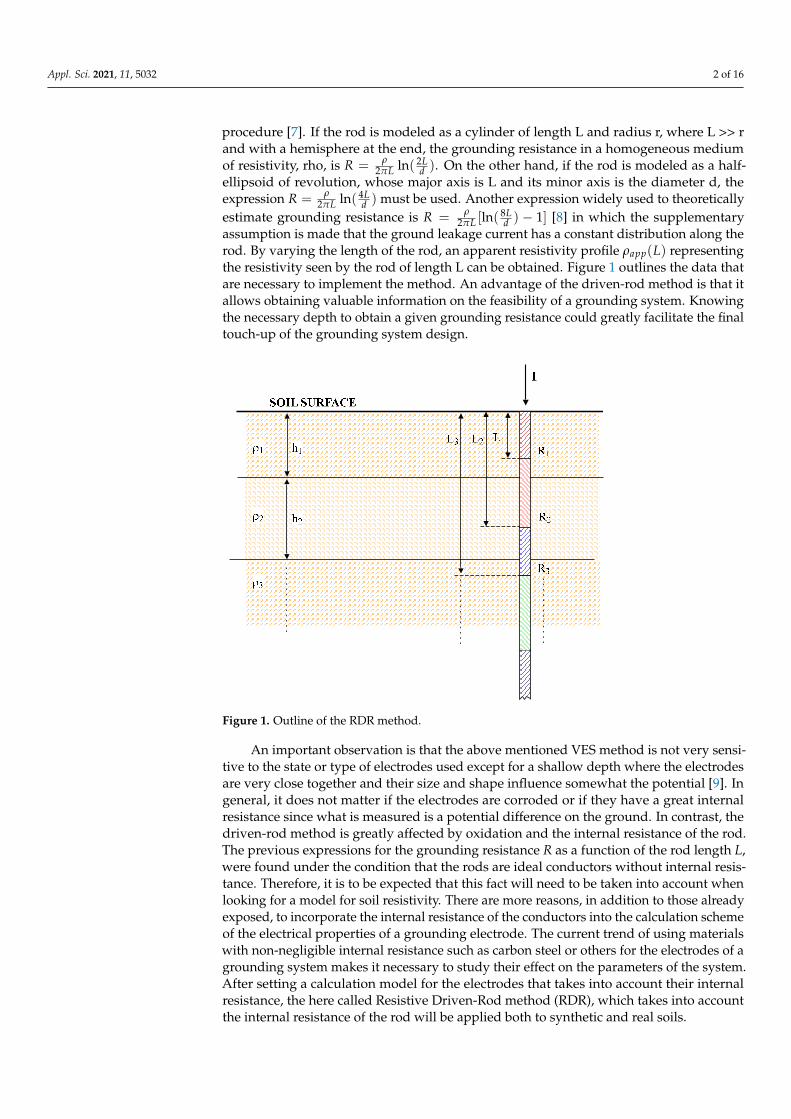
assumption is made that the ground leakage current has a constant distribution along therod. By varying the length of the rod, an apparent resistivity profile ρapp(L) representingthe resistivity seen by the rod of length L can be obtained. Figure 1 outlines the data thatare necessary to implement the method. An advantage of the driven-rod method is that itallows obtaining valuable information on the feasibility of a grounding system. Knowingthe necessary depth to obtain a given grounding resistance could greatly facilitate the finaltouch-up of the grounding system design.

Appl. Sci. 2021, 11, 5032 2 of 16

of vertical rods as grounding electrodes, such as in the case of lightning protection elec-trodes.

Another indirect procedure sometimes used is the driven-rod method. In this method, the grounding resistance of a rod driven into the ground is measured by the fall-of-potential procedure [7]. If the rod is modeled as a cylinder of length L and radius r, where L >> r and with a hemisphere at the end, the grounding resistance in a homogene-

ous medium of resistivity, rho, is 2ln( )2

LRL d

ρπ

= . On the other hand, if the rod is mod-

eled as a half-ellipsoid of revolution, whose major axis is L and its minor axis is the diam-

eter d, the expression 4ln( )2

LRL d

ρπ

= must be used. Another expression widely used to

theoretically estimate grounding resistance is 8[ln( ) 1]2

LRL d

ρπ

= − [8] in which the sup-

plementary assumption is made that the ground leakage current has a constant distribu-tion along the rod. By varying the length of the rod, an apparent resistivity profile ( )app Lρ representing the resistivity seen by the rod of length L can be obtained. Figure 1 outlines the data that are necessary to implement the method. An advantage of the driven-rod method is that it allows obtaining valuable information on the feasibility of a grounding system. Knowing the necessary depth to obtain a given grounding resistance could greatly facilitate the final touch-up of the grounding system design.

Figure 1. Outline of the RDR method.

An important observation is that the above mentioned VES method is not very sen-sitive to the state or type of electrodes used except for a shallow depth where the elec-trodes are very close together and their size and shape influence somewhat the potential [9]. In general, it does not matter if the electrodes are corroded or if they have a great internal resistance since what is measured is a potential difference on the ground. In con-trast, the driven-rod method is greatly affected by oxidation and the internal resistance of the rod. The previous expressions for the grounding resistance R as a function of the rod length L, were found under the condition that the rods are ideal conductors without in-ternal resistance. Therefore, it is to be expected that this fact will need to be taken into account when looking for a model for soil resistivity. There are more reasons, in addition to those already exposed, to incorporate the internal resistance of the conductors into the calculation scheme of the electrical properties of a grounding electrode. The current trend of using materials with non-negligible internal resistance such as carbon steel or others for the electrodes of a grounding system makes it necessary to study their effect on the

Figure 1. Outline of the RDR method.

An important observation is that the above mentioned VES method is not very sensi-tive to the state or type of electrodes used except for a shallow depth where the electrodesare very close together and their size and shape influence somewhat the potential [9]. Ingeneral, it does not matter if the electrodes are corroded or if they have a great internalresistance since what is measured is a potential difference on the ground. In contrast, thedriven-rod method is greatly affected by oxidation and the internal resistance of the rod.The previous expressions for the grounding resistance R as a function of the rod length L,were found under the condition that the rods are ideal conductors without internal resis-tance. Therefore, it is to be expected that this fact will need to be taken into account whenlooking for a model for soil resistivity. There are more reasons, in addition to those alreadyexposed, to incorporate the internal resistance of the conductors into the calculation schemeof the electrical properties of a grounding electrode. The current trend of using materialswith non-negligible internal resistance such as carbon steel or others for the electrodes of agrounding system makes it necessary to study their effect on the parameters of the system.After setting a calculation model for the electrodes that takes into account their internalresistance, the here called Resistive Driven-Rod method (RDR), which takes into accountthe internal resistance of the rod will be applied both to synthetic and real soils.

Appl. Sci. 2021, 11, 5032 3 of 16

A direct method to determine the resistivity as a function of the depth is knownin literature as normal resistivity logging (NRL) [10]. This is a geophysical method fordetermining the rock’s conductivity by studying the drilling geological profile in a well.However, this technique requires the drilling of a well of a section large enough for theprobes to be introduced. Resistivity is measured with a four-pin device taking a shortelectrode separation so that the well walls can be tested. To complete this brief reviewof several of the methods used to investigate the electrical structure of soils, mentionshould be made of the magnetic field-based eddy-current methods (ECM), framed inthe transient electromagnetic methods class. By means of a coil near the soil surface, avariable magnetic field is produced. Eddy-currents are generated in the conductive soil,producing magnetic fields that depend on the layer structure. Although they are basedon very different principles from those of the methods described so far, ECM are clearlynon-invasive methods with high resolution at shallow depth [11].

From the apparent resistivity data obtained with the indirect methods described above,the soil resistivity profile can be obtained by posing an inverse problem. Starting fromsemi-analytical expressions for the grounding resistance as a function of the parameters of amultilayer model, an optimization algorithm is implemented to find the set of parameters of themodel that minimizes the squared differences between the values of the resistance measuredin the field and those calculated with the theoretical expressions that contain the parameters.However, the techniques used in the inverse problem with the measurements made with theWenner array cannot be extended when the measurements come from a driven-rod logging.Apparent resistivity has a different meaning depending on the type of measurement.

The main objectives of this paper are, firstly, to establish a systematic procedure toinclude the internal resistance of conductors in the calculation of the grounding resistance ofburied electrodes, and secondly, testing the feasibility of the RDR method to determine theparameters of a multilayer soil model from grounding resistance measurements, pointingout its limitations. To achieve these goals, the paper is structured as follows. After thepresent introduction, the backgrounds section is intended to introduce the foundations ofthe proposed method. In the next section, some tests are carried out on synthetic soils inorder to test the method relevance. In the same section some real examples are also studied.Finally, the conclusions of the work are collected in the last section.

2. Modeling Grounding Electrodes with Internal Resistance: Backgrounds

The calculation of the grounding resistance of an electrode needs the model for theelectrical conductivity of the soil to be known. From a general point of view, it would

be necessary to solve the equation→∇ · (σ(→r )

→∇φ(

→r )) = 0 together with some boundary

conditions, where φ(→r ) is the absolute potential at the point

→r and σ(

→r ) represents the

conductivity of the ground. For a multilayered model it is possible to find acceptablesemi-analytical solutions for the potential. This model assumes that conductivity is justa non-continuous piecewise constant function. The soil is composed of horizontal layersof infinite extension and specific thickness in which the electrical conductivity takes aconstant and different value in each layer. Thus, the actual conductivity is replaced by astep function although in practice, due to the difficulty of the calculations, only a few layersare considered. The soil conductivity profiles of interest for this work comprise layers ofalmost any conductivity with thicknesses ranging from a few centimeters to tens of meters.Although for applications in grounding design it is common to deal with models in whichthe top layer is a few meters thick in which to place the grounding electrode.

Choosing a constant conductivity in each layer allows calculating the potential from theequation for a generic conductivity. The connection between the solutions corresponding toeach layer is made by imposing the continuity of the potential at the different interfaces aswell as the continuity of the normal component of the current density through interfaces.

Due to the supposed cylindrical symmetry of the potential, which is associated withconductivity dependent only on the depth as the z coordinate, the procedure to solvethe equation for the potential relies on using the method of separation of variables in a

Appl. Sci. 2021, 11, 5032 4 of 16

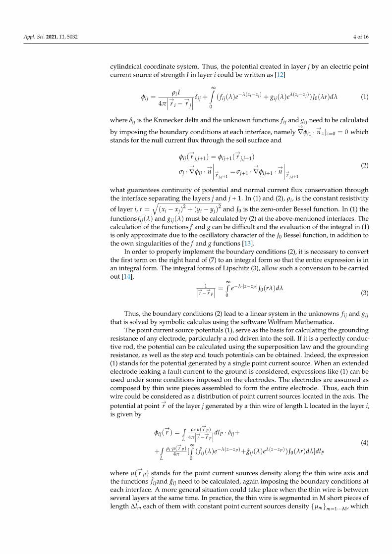
cylindrical coordinate system. Thus, the potential created in layer j by an electric pointcurrent source of strength I in layer i could be written as [12]

φij =ρi I

4π∣∣∣→r i −

→r j

∣∣∣ δij +

∞∫0

( fij(λ)e−λ(zi−zj) + gij(λ)e

λ(zi−zj))J0(λr)dλ (1)

where δij is the Kronecker delta and the unknown functions fij and gij need to be calculated

by imposing the boundary conditions at each interface, namely→∇φi1 ·

→n z|z=0 = 0 which

stands for the null current flux through the soil surface and

φij(→r j,j+1) = φij+1(

→r j,j+1)

σj ·→∇φij ·

→n∣∣∣∣→r j,j+1

=σj+1 ·→∇φij+1 ·

→n∣∣∣∣→r j,j+1

(2)

what guarantees continuity of potential and normal current flux conservation throughthe interface separating the layers j and j + 1. In (1) and (2), ρi, is the constant resistivity

of layer i, r =√(xi − xj)

2 + (yi − yj)2 and J0 is the zero-order Bessel function. In (1) the

functions fij(λ) and gij(λ) must be calculated by (2) at the above-mentioned interfaces. Thecalculation of the functions f and g can be difficult and the evaluation of the integral in (1)is only approximate due to the oscillatory character of the J0 Bessel function, in addition tothe own singularities of the f and g functions [13].

In order to properly implement the boundary conditions (2), it is necessary to convertthe first term on the right hand of (7) to an integral form so that the entire expression is inan integral form. The integral forms of Lipschitz (3), allow such a conversion to be carriedout [14],

1∣∣∣→r −→r P

∣∣∣ =∞∫0

e−λ·|z−zP | J0(rλ)dλ(3)

Thus, the boundary conditions (2) lead to a linear system in the unknowns fij and gijthat is solved by symbolic calculus using the software Wolfram Mathematica.

The point current source potentials (1), serve as the basis for calculating the groundingresistance of any electrode, particularly a rod driven into the soil. If it is a perfectly conduc-tive rod, the potential can be calculated using the superposition law and the groundingresistance, as well as the step and touch potentials can be obtained. Indeed, the expression(1) stands for the potential generated by a single point current source. When an extendedelectrode leaking a fault current to the ground is considered, expressions like (1) can beused under some conditions imposed on the electrodes. The electrodes are assumed ascomposed by thin wire pieces assembled to form the entire electrode. Thus, each thinwire could be considered as a distribution of point current sources located in the axis. Thepotential at point

→r of the layer j generated by a thin wire of length L located in the layer i,

is given by

φij(→r ) =

∫L

ρi ·µ(→r P)

4π∣∣∣→r −→r P

∣∣∣dlP · δij+

+∫L

ρi ·µ(→r P)

4π [∞∫0( fij(λ)e−λ(z−zP)+gij(λ)eλ(z−zP))J0(λr)dλ]dlP

(4)

where µ(→r P) stands for the point current sources density along the thin wire axis and

the functions fijand gij need to be calculated, again imposing the boundary conditions ateach interface. A more general situation could take place when the thin wire is betweenseveral layers at the same time. In practice, the thin wire is segmented in M short pieces oflength ∆lm each of them with constant point current sources density µmm=1···M, which

Appl. Sci. 2021, 11, 5032 5 of 16

are used to calculate the potential of the electrode itself by imposing a constant value ofsuch potential along the entire electrode, the grounding electrode potential [15]. Thus, thepotential at point

→r of the layer j becomes:

φ(→r j) =

M∑

m=1

ρm ·µm ·∆lm4π∣∣∣→r j−

→r m

∣∣∣ δmj+

+M∑

m=1

ρm ·µm ·∆lm4π

∞∫0( fmj(λ)e

−λ(zj−zm)+gmj(λ)eλ(zj−zm))J0(λr)dλ

(5)

This procedure, known as moment method, gives rise to a system of linear equationswhose unknowns are the constant densities µmm=1···M of point current sources in eachsegment [16]. The knowledge of these densities allows the calculation of the potentialat any point on the ground by superposition. The electrode potential itself is of specialinterest for this work. As it was pointed out, it is obtained as a part of the solution for theµk densities and then the grounding resistance can be easily calculated.

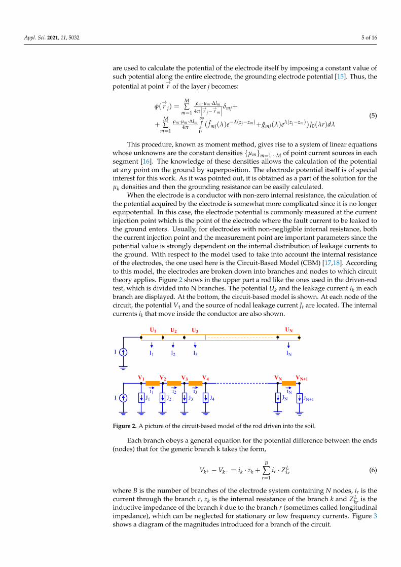
When the electrode is a conductor with non-zero internal resistance, the calculation ofthe potential acquired by the electrode is somewhat more complicated since it is no longerequipotential. In this case, the electrode potential is commonly measured at the currentinjection point which is the point of the electrode where the fault current to be leaked tothe ground enters. Usually, for electrodes with non-negligible internal resistance, boththe current injection point and the measurement point are important parameters since thepotential value is strongly dependent on the internal distribution of leakage currents tothe ground. With respect to the model used to take into account the internal resistanceof the electrodes, the one used here is the Circuit-Based Model (CBM) [17,18]. Accordingto this model, the electrodes are broken down into branches and nodes to which circuittheory applies. Figure 2 shows in the upper part a rod like the ones used in the driven-rodtest, which is divided into N branches. The potential Uk and the leakage current Ik in eachbranch are displayed. At the bottom, the circuit-based model is shown. At each node of thecircuit, the potential Vt and the source of nodal leakage current Jt are located. The internalcurrents ik that move inside the conductor are also shown.

Appl. Sci. 2021, 11, 5032 5 of 16

where ( )Prμ stands for the point current sources density along the thin wire axis and the

functions ijf and ˆ ijg need to be calculated, again imposing the boundary conditions at each interface. A more general situation could take place when the thin wire is between several layers at the same time. In practice, the thin wire is segmented in M short pieces of length mlΔ each of them with constant point current sources density 1m m Mμ

= , which are used to calculate the potential of the electrode itself by imposing a constant value of such potential along the entire electrode, the grounding electrode potential [15]. Thus, the potential at point r of the layer j becomes:

1

( ) ( )0

1 0

( )4

ˆ ˆ( ( ) ( ) ) ( )4

j m j m

Mm m m

j mjm j m

Mz z z zm m m

mj mjm

lrr r

l f e g e J r dλ λ

ρ μφ δπ

ρ μ λ λ λ λπ

=

∞− − −

=

⋅ ⋅Δ= +

−

⋅ ⋅Δ+ +

(5)

This procedure, known as moment method, gives rise to a system of linear equations whose unknowns are the constant densities 1m m Mμ

= of point current sources in each segment [16]. The knowledge of these densities allows the calculation of the potential at any point on the ground by superposition. The electrode potential itself is of special interest for this work. As it was pointed out, it is obtained as a part of the solution for the

kμ densities and then the grounding resistance can be easily calculated. When the electrode is a conductor with non-zero internal resistance, the calculation

of the potential acquired by the electrode is somewhat more complicated since it is no longer equipotential. In this case, the electrode potential is commonly measured at the current injection point which is the point of the electrode where the fault current to be leaked to the ground enters. Usually, for electrodes with non-negligible internal re-sistance, both the current injection point and the measurement point are important pa-rameters since the potential value is strongly dependent on the internal distribution of leakage currents to the ground. With respect to the model used to take into account the internal resistance of the electrodes, the one used here is the Circuit-Based Model (CBM) [17,18]. According to this model, the electrodes are broken down into branches and nodes to which circuit theory applies. Figure 2 shows in the upper part a rod like the ones used in the driven-rod test, which is divided into N branches. The potential Uk and the leakage current Ik in each branch are displayed. At the bottom, the circuit-based model is shown. At each node of the circuit, the potential Vt and the source of nodal leakage current Jt are located. The internal currents ik that move inside the conductor are also shown.

Figure 2. A picture of the circuit-based model of the rod driven into the soil.

Each branch obeys a general equation for the potential difference between the ends (nodes) that for the generic branch k takes the form,

I I1 I2 I3 IN

U1 U2 U3 UN

Ii1

V1 V2 V3 VNV4 VN+1

J1

i2 i3 iNJ2 J3 J4 JN+1JN

Figure 2. A picture of the circuit-based model of the rod driven into the soil.

Each branch obeys a general equation for the potential difference between the ends(nodes) that for the generic branch k takes the form,

Vk+ −Vk− = ik · zk +B

∑r=1

ir · ZLkr (6)

where B is the number of branches of the electrode system containing N nodes, ir is thecurrent through the branch r, zk is the internal resistance of the branch k and ZL

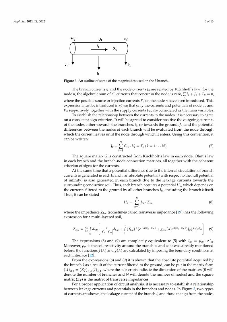
kr is theinductive impedance of the branch k due to the branch r (sometimes called longitudinalimpedance), which can be neglected for stationary or low frequency currents. Figure 3shows a diagram of the magnitudes introduced for a branch of the circuit.

Appl. Sci. 2021, 11, 5032 6 of 16

Appl. Sci. 2021, 11, 5032 6 of 16

1

BL

k k r krk kr

V V i z i Z+ −

=

− = ⋅ + ⋅ (6)

where B is the number of branches of the electrode system containing N nodes, ir is the current through the branch r, zk is the internal resistance of the branch k and L

krZ is the inductive impedance of the branch k due to the branch r (sometimes called longitudinal impedance), which can be neglected for stationary or low frequency currents. Figure 3 shows a diagram of the magnitudes introduced for a branch of the circuit.

Figure 3. An outline of some of the magnitudes used on the k branch.

The branch currents ik and the node currents Jn are related by Kirchhoff’s law: for the node n, the algebraic sum of all currents that concur in the node is zero, 0k n n

ni J F+ + =

, where the possible source or injection currents Fn on the node n have been introduced. This expression must be introduced in (6) so that only the currents and potentials of node, Jn and Vn respectively, together with the supply currents Fn, are considered as the main variables.

To establish the relationship between the currents in the nodes, it is necessary to agree on a consistent sign criterion. It will be agreed to consider positive the outgoing currents of the nodes either towards the branches, ik, or towards the ground, Jn, and the potential differences between the nodes of each branch will be evaluated from the node through which the current leaves until the node through which it enters. Using this convention, it can be written:

1 ( 1 )

N

k lk l kl

J G V F k N=

+ ⋅ = = (7)

The square matrix G is constructed from Kirchhoff’s law in each node, Ohm’s law in each branch and the branch-node connection matrices, all together with the coherent cri-terion of signs for the currents.

At the same time that a potential difference due to the internal circulation of branch currents is generated in each branch, an absolute potential (with respect to the null poten-tial of infinity) is also generated in each branch due to the leakage currents towards the surrounding conductive soil. Thus, each branch acquires a potential Uk, which depends on the currents filtered to the ground by all other branches Im, including the branch k itself. Thus, it can be stated

1

B

k m kmm

U I Z=

= ⋅ (8)

where the impedance Zkm (sometimes called transverse impedance [19]) has the following expression for a multi-layered soil,

(z ) (z )0

0

1 ( ( ) ( ) ) ( )4

k m k m

m

z zmkm m km km km

k ml

Z dl f e g e J r dr r

λ λρ δ λ λ λ λπ

∞− − −

= + + − (9)

Figure 3. An outline of some of the magnitudes used on the k branch.

The branch currents ik and the node currents Jn are related by Kirchhoff’s law: for thenode n, the algebraic sum of all currents that concur in the node is zero, ∑

nik + Jn + Fn = 0,

where the possible source or injection currents Fn on the node n have been introduced. Thisexpression must be introduced in (6) so that only the currents and potentials of node, Jn andVn respectively, together with the supply currents Fn, are considered as the main variables.

To establish the relationship between the currents in the nodes, it is necessary to agreeon a consistent sign criterion. It will be agreed to consider positive the outgoing currentsof the nodes either towards the branches, ik, or towards the ground, Jn, and the potentialdifferences between the nodes of each branch will be evaluated from the node throughwhich the current leaves until the node through which it enters. Using this convention, itcan be written:

Jk +N

∑l=1

Glk ·Vl = Fk (k = 1 · · ·N) (7)

The square matrix G is constructed from Kirchhoff’s law in each node, Ohm’s lawin each branch and the branch-node connection matrices, all together with the coherentcriterion of signs for the currents.

At the same time that a potential difference due to the internal circulation of branchcurrents is generated in each branch, an absolute potential (with respect to the null potentialof infinity) is also generated in each branch due to the leakage currents towards thesurrounding conductive soil. Thus, each branch acquires a potential Uk, which depends onthe currents filtered to the ground by all other branches Im, including the branch k itself.Thus, it can be stated

Uk =B

∑m=1

Im · Zkm (8)

where the impedance Zkm (sometimes called transverse impedance [19]) has the followingexpression for a multi-layered soil,

Zkm = ρm4π

∫lm

dlm

[1∣∣∣→r k−→r m

∣∣∣ δkm +∞∫0( fkm(λ)e−λ(zk−zm) + gkm(λ)eλ(zk−zm))J0(λr)dλ

](9)

The expressions (8) and (9) are completely equivalent to (5) with Im = µm · ∆lm.Moreover, ρm is the soil resistivity around the branch m and as it was already mentionedbefore, the functions f (λ) and g(λ) are calculated by imposing the boundary conditions ateach interface [12].

From the expressions (8) and (9) it is shown that the absolute potential acquired bythe branch k as a result of the current filtered to the ground, can be put in the matrix form(U)B,1 = (ZT)B,B(I)B,1, where the subscripts indicate the dimension of the matrices (B willdenote the number of branches and N will denote the number of nodes) and the squarematrix (ZT) is the matrix of transverse impedances.

For a proper application of circuit analysis, it is necessary to establish a relationshipbetween leakage currents and potentials in the branches and nodes. In Figure 3, two typesof currents are shown, the leakage current of the branch Ii and those that go from the nodes

Appl. Sci. 2021, 11, 5032 7 of 16

of the branch Jk+ y Jk-, both towards the surrounding medium. It will be agreed that bothnode and branch currents to the surrounding medium are related by the matrix equation

(J)N,1 = (C)N,B · (I)B,1 (10)

where (C) is a matrix of N rows (nodes) and B columns (branches) whose elements are

cij =

1/2 if the node i is connected to the branch j0 otherwise

(11)

This means that each branch leakage current Ii is divided into two halves that go tothe currents of nodes Ji+ and Ji− . With regard to the branch potential Ui and the potentialsof the branch nodes Vi

+ and Vi−,

(U)B,1 = (K)B,N · (V)N,1 (12)

with (K) being a matrix of B rows (branches) and N columns (nodes), whose elements are

kij =

1/2 if the branch i is connected to the node j0 otherwise

(13)

which really means that the branch potential is the average value of the potentials of itsnodes Ui =

Vn+Vn+12 . With Equations (7), (8), (10) and (12) a system of matrix equations can

be proposed,(J)N,1 + (G)N,N · (V)N,1 = (F)N,1(U)B,1 = (Z)B,B · (I)B,1(J)N,1 = (C)N,B · (I)B,1(U)B,1 = (K)B,N · (V)N,1

(14)

Defining a vector of unknowns consisting of currents and potentials In y Vn

(W)B+N,1 =

((I)B,1

(V)N,1

)(15)

the system of Equation (14) can be written as((Z)B,B −(K)B,N(C)N,B (G)N,N

)· (W)N+B,1 =

((0)B,1

(F)N,1

)(16)

which allows us to find the solution of the problem in terms of potentials and currents.The electrode potential is the one corresponding to the node through which the current

enters the electrode and the grounding resistance is the quotient between this potentialand the injected current. Note that both depend on the parameters of the multilayer modelchosen through ρm and the functions f (λ) and g(λ) in (9).

For an L length rod driven into the soil of parameters ρ1, ρ2 . . . , h1, h2 . . ., the calcu-lated grounding resistance will be denoted as Rcalc(L; ρ1, ρ2 . . . , h1, h2 . . .). In practice,a direct measurement in the field of the grounding resistance Rmeas of the rod by the fall-of-potential method is performed. The control variable is the rod length L, thus a set ofgrounding resistance values corresponding to increasing lengths of the rod are available.From these measurements an optimization algorithm that minimizes

χ2 = ∑j[Rmeas(Lj)− Rcalc(Lj; ρ1, ρ2 . . . , h1, h2 . . .)]2 (17)

could be implemented. This problem falls into the category of so-called inverse problems,which are very often ill-conditioned. That means in practice that uncertainties in themeasurements of grounding resistance can led to very dramatic changes in the parameter

Appl. Sci. 2021, 11, 5032 8 of 16

values of the multilayered model. Consequently, there may be no single solution to theresistivity profile from the measured grounding resistance series.

To finish this section, some considerations about the model presented here will be dis-cussed. The internal resistance of a grounding electrode plays an important role for severalreasons. In the first place, as already mentioned, the electrode is no longer equipotential,and the grounding resistance must be defined as indicated above. The current injectionpoint is an important choice and must be chosen so that its potential is as low as possible.Second, the calculations made with this model allow validating or discarding materials tobe used in electrodes on condition of verifying technical requirements on the value of thegrounding resistance and the step and touch potentials required in an installation. Notethat increasing the size of the electrodes can help to decrease the grounding resistance aslong as the internal resistance of the conductors does not result in a final increase in thegrounding resistance. Finally, another effect to consider that can only be evaluated withmodels such as the one presented here is the heating by the Joule effect on the electrodes.The heat generated can cause an unwanted increase in grounding resistance when takinginto account the variation in resistivity with temperature. The effect must be studied andonly models that take into account the internal resistivity of the conductors are valid forthis purpose.

3. Application to Resistive Driven-Rod Method: Testing with Some Examples

In the tests that will be described below, a rod is vertically driven into a multilayersoil and the grounding resistance is measured as a function of the length of the rod thatis buried in the soil. According to the circuit-based model introduced in Section 2, eachbranch of the buried rod contributes with a leakage current leakage to the ground andelectric potentials are generated at its ends that must be determined by solving (16). Thegrounding resistance can be calculated from the potential acquired by the injection point ofthe total current, which is usually the upper end of the rod. This potential depends on theinternal resistance of the rod and the resistivity profile of the ground through the resistivityand width of the different layers. These soil parameters can be found by a minimizationprocedure of (17). In order to work in conditions similar to the real tests, some additionalconsiderations need to be discussed.

First of all, it is necessary to comment that in many real cases, the rod driven intothe soil is composed of rod segments of fixed length assembled by means of small joiningpieces. Such connecting pieces provide a contact resistance between the two rods that arejoined that makes the whole rod a conductor with non-zero internal resistance. This factwill be modeled by associating a non-zero resistivity to the connecting piece between theadjacent rods, the rods themselves being ideal conductors. Each time a rod segment isassembled with a joining piece and driven into the ground, the grounding resistance of theentire rod is measured. For practical reasons, the rod segments usually have a size rangingfrom 1 m to 1.5 m while the connecting pieces have a length of a few centimeters. In someof the synthetic cases that will be studied, 0.5 m rod segments will be used although thissize is actually fictitious.

3.1. Synthetic Examples with No Internal Resistance

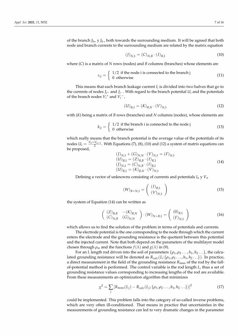
Let us consider first a synthetic example in which the rod has no internal resistance.Let the ground be a synthetic three-layer soil with parameters ρ1 = 100 Ωm, ρ2 = 50 Ωm,ρ3 = 300 Ωm, h1 = 2 m, and h2 = 3 m, where a vertical zero-resistive rod of 9 mm radius isdriven into the soil from 0.5 m up to 8 m deep. The rod is assumed to be made of a singlecontinuous piece that is introduced in segments of 0.5 m in the ground. For every 0.5 mof drilling, the grounding resistance is calculated assuming that it is a value obtained in afield measurement using the fall-of-potential method. Table 1 shows the results where L isin meters and R is in Ohms.

Appl. Sci. 2021, 11, 5032 9 of 16

Table 1. Buried rod length L (m) and the corresponding grounding resistance R (Ω).

L (m) 0.5 1 1.5 2 2.5 3 3.5 4

R (Ω) 139.90 80.67 57.79 44.68 31.74 25.52 21.66 19.05

L (m) 4.5 5 5.5 6 6.5 7 7.5 8.0

R (Ω) 17.18 15.97 15.76 15.54 15.31 15.07 14.85 14.62

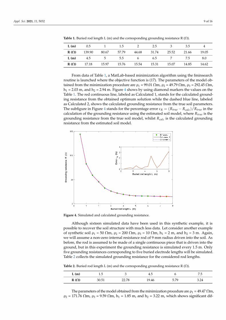
From data of Table 1, a MatLab-based minimization algorithm using the fminsearchroutine is launched where the objective function is (17). The parameters of the model ob-tained from the minimization procedure are ρ1 = 99.01 Ωm, ρ2 = 49.79 Ωm, ρ3 = 292.45 Ωm,h1 = 2.03 m, and h2 = 2.94 m. Figure 4 shows by using diamond markers the values on theTable 1. The red continuous line, labeled as Calculated 1, stands for the calculated ground-ing resistance from the obtained optimum solution while the dashed blue line, labeledas Calculated 2, shows the calculated grounding resistance from the true soil parameters.The subfigure in Figure 4 stands for the percentage error εR = (Rtrue − Rcalc)/Rtrue in thecalculation of the grounding resistance using the estimated soil model, where Rtrue is thegrounding resistance from the true soil model, whilst Rcalc is the calculated groundingresistance from the estimated soil model.

Appl. Sci. 2021, 11, 5032 9 of 16

In some of the synthetic cases that will be studied, 0.5 m rod segments will be used alt-hough this size is actually fictitious.

3.1. Synthetic Examples with No Internal Resistance Let us consider first a synthetic example in which the rod has no internal resistance.

Let the ground be a synthetic three-layer soil with parameters ρ1 = 100 Ωm, ρ2 = 50 Ωm, ρ3

= 300 Ωm, h1 = 2 m, and h2 = 3 m, where a vertical zero-resistive rod of 9 mm radius is driven into the soil from 0.5 m up to 8 m deep. The rod is assumed to be made of a single continuous piece that is introduced in segments of 0.5 m in the ground. For every 0.5 m of drilling, the grounding resistance is calculated assuming that it is a value obtained in a field measurement using the fall-of-potential method. Table 1 shows the results where L is in meters and R is in Ohms.

Table 1. Buried rod length L (m) and the corresponding grounding resistance R (Ω).

L(m) 0.5 1 1.5 2 2.5 3 3.5 4 R(Ω) 139.90 80.67 57.79 44.68 31.74 25.52 21.66 19.05 L(m) 4.5 5 5.5 6 6.5 7 7.5 8.0 R(Ω) 17.18 15.97 15.76 15.54 15.31 15.07 14.85 14.62

From data of Table 1, a MatLab-based minimization algorithm using the fminsearch routine is launched where the objective function is (17). The parameters of the model ob-tained from the minimization procedure are ρ1 = 99.01 Ωm, ρ2 = 49.79 Ωm, ρ3 = 292.45 Ωm, h1 = 2.03 m, and h2 = 2.94 m. Figure 4 shows by using diamond markers the values on the Table 1. The red continuous line, labeled as Calculated 1, stands for the calculated ground-ing resistance from the obtained optimum solution while the dashed blue line, labeled as Calculated 2, shows the calculated grounding resistance from the true soil parameters. The subfigure in Figure 4 stands for the percentage error ( ) /R true calc trueR R Rε = − in the calculation of the grounding resistance using the estimated soil model, where trueR is the grounding resistance from the true soil model, whilst calcR is the calculated grounding resistance from the estimated soil model.

Figure 4. Simulated and calculated grounding resistance.

Although sixteen simulated data have been used in this synthetic example, it is pos-sible to recover the soil structure with much less data. Let consider another example of synthetic soil ρ1 = 50 Ωm, ρ2 = 200 Ωm, ρ3 = 10 Ωm, h1 = 2 m, and h2 = 3 m. Again, we will assume a non-zero internal resistance rod of 9 mm radius driven into the soil. As before,

Figure 4. Simulated and calculated grounding resistance.

Although sixteen simulated data have been used in this synthetic example, it ispossible to recover the soil structure with much less data. Let consider another exampleof synthetic soil ρ1 = 50 Ωm, ρ2 = 200 Ωm, ρ3 = 10 Ωm, h1 = 2 m, and h2 = 3 m. Again,we will assume a non-zero internal resistance rod of 9 mm radius driven into the soil. Asbefore, the rod is assumed to be made of a single continuous piece that is driven into theground, but in this experiment the grounding resistance is simulated every 1.5 m. Onlyfive grounding resistances corresponding to five buried electrode lengths will be simulated.Table 2 collects the simulated grounding resistance for the considered rod lengths.

Table 2. Buried rod length L (m) and the corresponding grounding resistance R (Ω).

L (m) 1.5 3 4.5 6 7.5

R (Ω) 30.51 22.78 19.46 5.79 3.24

The parameters of the model obtained from the minimization procedure are ρ1 = 49.47 Ωm,ρ2 = 171.76 Ωm, ρ3 = 9.59 Ωm, h1 = 1.85 m, and h2 = 3.22 m, which shows significant dif-

Appl. Sci. 2021, 11, 5032 10 of 16

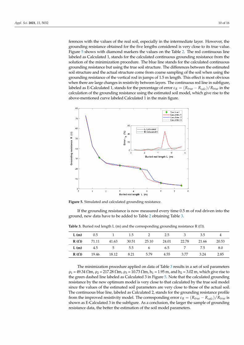
ferences with the values of the real soil, especially in the intermediate layer. However, thegrounding resistance obtained for the five lengths considered is very close to its true value.Figure 5 shows with diamond markers the values on the Table 2. The red continuous linelabeled as Calculated 1, stands for the calculated continuous grounding resistance from thesolution of the minimization procedure. The blue line stands for the calculated continuousgrounding resistance but using the true soil structure. The differences between the estimatedsoil structure and the actual structure come from coarse sampling of the soil when using thegrounding resistance of the vertical rod in jumps of 1.5 m length. This effect is most obviouswhen there are large changes in resistivity between layers. The continuous red line in subfigure,labeled as E-Calculated 1, stands for the percentage of error εR = (Rtrue − Rcalc)/Rtrue in thecalculation of the grounding resistance using the estimated soil model, which give rise to theabove-mentioned curve labeled Calculated 1 in the main figure.

Appl. Sci. 2021, 11, 5032 10 of 16

the rod is assumed to be made of a single continuous piece that is driven into the ground, but in this experiment the grounding resistance is simulated every 1.5 m. Only five grounding resistances corresponding to five buried electrode lengths will be simulated. Table 2 collects the simulated grounding resistance for the considered rod lengths.

Table 2. Buried rod length L (m) and the corresponding grounding resistance R (Ω).

L(m) 1.5 3 4.5 6 7.5 R(Ω) 30.51 22.78 19.46 5.79 3.24

The parameters of the model obtained from the minimization procedure are ρ1 = 49.47 Ωm, ρ2 = 171.76 Ωm, ρ3 = 9.59 Ωm, h1 = 1.85 m, and h2 = 3.22 m, which shows significant differences with the values of the real soil, especially in the intermediate layer. However, the grounding resistance obtained for the five lengths considered is very close to its true value. Figure 5 shows with diamond markers the values on the Table 2. The red continu-ous line labeled as Calculated 1, stands for the calculated continuous grounding resistance from the solution of the minimization procedure. The blue line stands for the calculated continuous grounding resistance but using the true soil structure. The differences between the estimated soil structure and the actual structure come from coarse sampling of the soil when using the grounding resistance of the vertical rod in jumps of 1.5 m length. This effect is most obvious when there are large changes in resistivity between layers. The con-tinuous red line in subfigure, labeled as E-Calculated 1, stands for the percentage of error

( ) /R true calc trueR R Rε = − in the calculation of the grounding resistance using the estimated soil model, which give rise to the above-mentioned curve labeled Calculated 1 in the main figure.

Figure 5. Simulated and calculated grounding resistance.

If the grounding resistance is now measured every time 0.5 m of rod driven into the ground, new data have to be added to Table 2 obtaining Table 3.

Table 3. Buried rod length L (m) and the corresponding grounding resistance R (Ω).

L(m) 0.5 1 1.5 2 2.5 3 3.5 4 R(Ω) 71.11 41.63 30.51 25.10 24.01 22.78 21.66 20.53 L(m) 4.5 5 5.5 6 6.5 7 7.5 8.0 R(Ω) 19.46 18.12 8.21 5.79 4.55 3.77 3.24 2.85

Gro

undi

ng re

sist

ance

R (

)

Erro

r R

(%

)

Figure 5. Simulated and calculated grounding resistance.

If the grounding resistance is now measured every time 0.5 m of rod driven into theground, new data have to be added to Table 2 obtaining Table 3.

Table 3. Buried rod length L (m) and the corresponding grounding resistance R (Ω).

L (m) 0.5 1 1.5 2 2.5 3 3.5 4

R (Ω) 71.11 41.63 30.51 25.10 24.01 22.78 21.66 20.53

L (m) 4.5 5 5.5 6 6.5 7 7.5 8.0

R (Ω) 19.46 18.12 8.21 5.79 4.55 3.77 3.24 2.85

The minimization procedure applied on data of Table 3 results in a set of soil parametersρ1 = 49.34 Ωm, ρ2 = 217.28 Ωm, ρ3 = 10.73 Ωm, h1 = 1.95 m, and h2 = 3.02 m, which give rise tothe green dashed line labeled as Calculated 3 in Figure 5. Note that the calculated groundingresistance by the new optimum model is very close to that calculated by the true soil modelsince the values of the estimated soil parameters are very close to those of the actual soil.The continuous blue line, labeled as Calculated 2, stands for the grounding resistance profilefrom the improved resistivity model. The corresponding error εR = (Rtrue − Rcalc)/Rtrue isshown as E-Calculated 3 in the subfigure. As a conclusion, the larger the sample of groundingresistance data, the better the estimation of the soil model parameters.

Appl. Sci. 2021, 11, 5032 11 of 16

3.2. Synthetic Examples with Internal Resistance

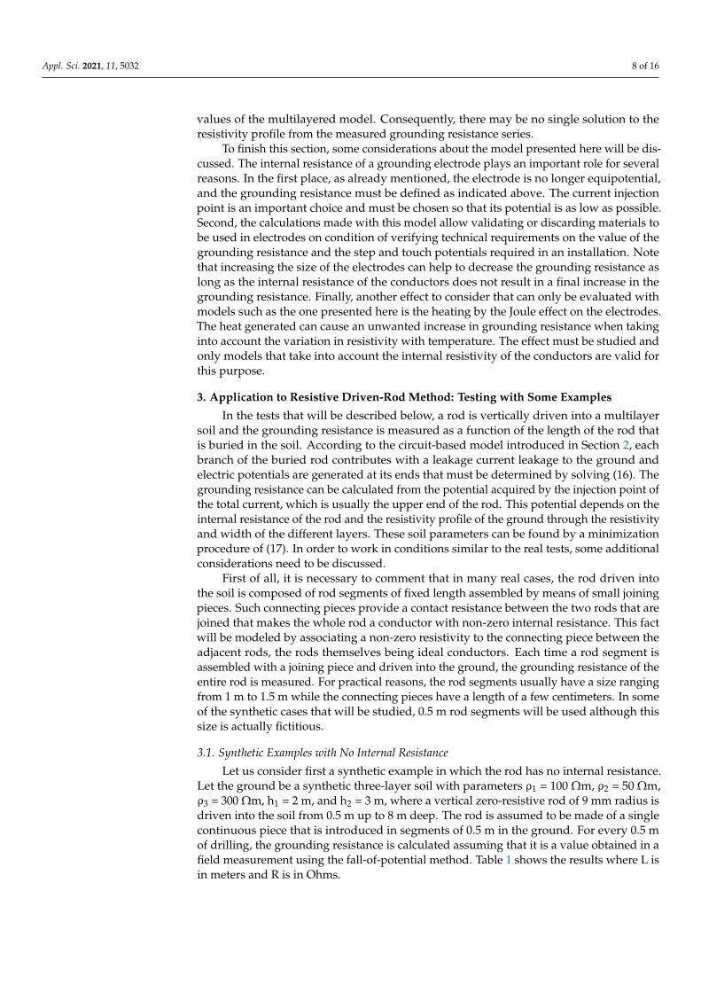
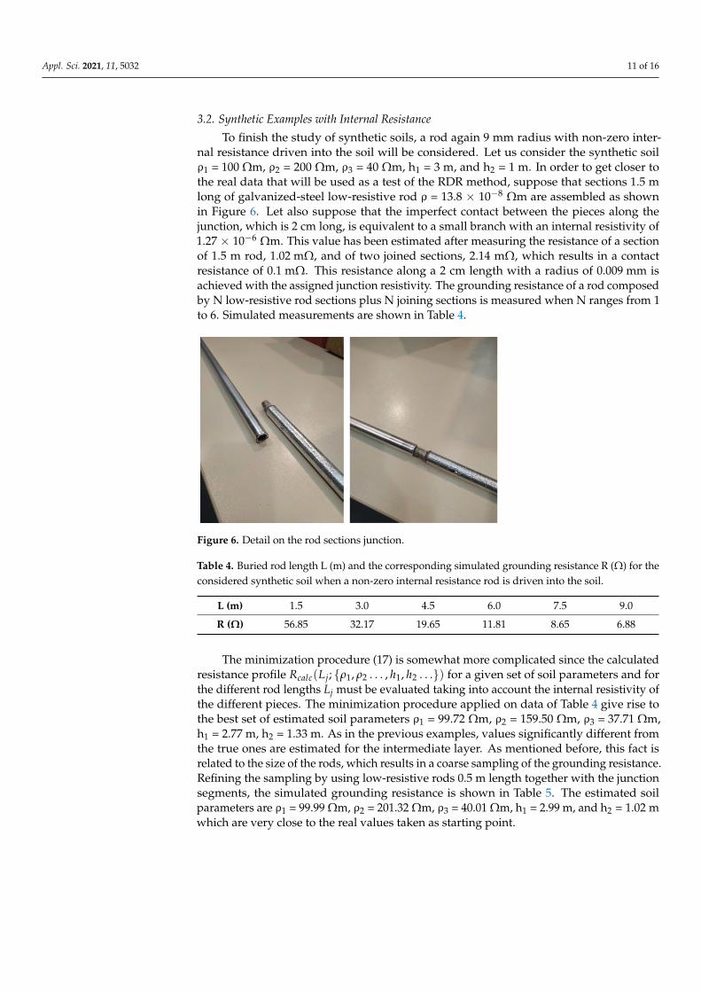
To finish the study of synthetic soils, a rod again 9 mm radius with non-zero inter-nal resistance driven into the soil will be considered. Let us consider the synthetic soilρ1 = 100 Ωm, ρ2 = 200 Ωm, ρ3 = 40 Ωm, h1 = 3 m, and h2 = 1 m. In order to get closer tothe real data that will be used as a test of the RDR method, suppose that sections 1.5 mlong of galvanized-steel low-resistive rod ρ = 13.8 × 10−8 Ωm are assembled as shownin Figure 6. Let also suppose that the imperfect contact between the pieces along thejunction, which is 2 cm long, is equivalent to a small branch with an internal resistivity of1.27 × 10−6 Ωm. This value has been estimated after measuring the resistance of a sectionof 1.5 m rod, 1.02 mΩ, and of two joined sections, 2.14 mΩ, which results in a contactresistance of 0.1 mΩ. This resistance along a 2 cm length with a radius of 0.009 mm isachieved with the assigned junction resistivity. The grounding resistance of a rod composedby N low-resistive rod sections plus N joining sections is measured when N ranges from 1to 6. Simulated measurements are shown in Table 4.

Appl. Sci. 2021, 11, 5032 11 of 16

L(m) 4.5 5 5.5 6 6.5 7 7.5 8.0 R(Ω) 19.46 18.12 8.21 5.79 4.55 3.77 3.24 2.85

The minimization procedure applied on data of Table 3 results in a set of soil param-eters ρ1 = 49.34 Ωm, ρ2 = 217.28 Ωm, ρ3 = 10.73 Ωm, h1 = 1.95 m, and h2 = 3.02 m, which give rise to the green dashed line labeled as Calculated 3 in Figure 5. Note that the calculated grounding resistance by the new optimum model is very close to that calculated by the true soil model since the values of the estimated soil parameters are very close to those of the actual soil. The continuous blue line, labeled as Calculated 2, stands for the grounding resistance profile from the improved resistivity model. The corresponding error

( ) /R true calc trueR R Rε = − is shown as E-Calculated 3 in the subfigure. As a conclusion, the larger the sample of grounding resistance data, the better the estimation of the soil model parameters.

3.2. Synthetic Examples with Internal Resistance To finish the study of synthetic soils, a rod again 9 mm radius with non-zero internal

resistance driven into the soil will be considered. Let us consider the synthetic soil ρ1 = 100 Ωm, ρ2 = 200 Ωm, ρ3 = 40 Ωm, h1 = 3 m, and h2 = 1 m. In order to get closer to the real data that will be used as a test of the RDR method, suppose that sections 1.5 m long of galva-nized-steel low-resistive rod ρ = 13.8 × 10−8 Ωm are assembled as shown in Figure 6. Let also suppose that the imperfect contact between the pieces along the junction, which is 2 cm long, is equivalent to a small branch with an internal resistivity of 1.27 × 10−6 Ωm. This value has been estimated after measuring the resistance of a section of 1.5 m rod, 1.02 mΩ, and of two joined sections, 2.14 mΩ, which results in a contact resistance of 0.1 mΩ. This resistance along a 2 cm length with a radius of 0.009 mm is achieved with the assigned junction resistivity. The grounding resistance of a rod composed by N low-resistive rod sections plus N joining sections is measured when N ranges from 1 to 6. Simulated meas-urements are shown in Table 4.

Figure 6. Detail on the rod sections junction.

Table 4. Buried rod length L (m) and the corresponding simulated grounding resistance R (Ω) for the considered synthetic soil when a non-zero internal resistance rod is driven into the soil.

L(m) 1.5 3.0 4.5 6.0 7.5 9.0 R(Ω) 56.85 32.17 19.65 11.81 8.65 6.88

The minimization procedure (17) is somewhat more complicated since the calculated resistance profile 1 2 1 2( ; , ..., , ... )calc jR L h hρ ρ for a given set of soil parameters and for the different rod lengths Lj must be evaluated taking into account the internal resistivity of the different pieces. The minimization procedure applied on data of Table 4 give rise to the best set of estimated soil parameters ρ1 = 99.72 Ωm, ρ2 = 159.50 Ωm, ρ3 = 37.71 Ωm, h1 =

Figure 6. Detail on the rod sections junction.

Table 4. Buried rod length L (m) and the corresponding simulated grounding resistance R (Ω) for theconsidered synthetic soil when a non-zero internal resistance rod is driven into the soil.

L (m) 1.5 3.0 4.5 6.0 7.5 9.0

R (Ω) 56.85 32.17 19.65 11.81 8.65 6.88

The minimization procedure (17) is somewhat more complicated since the calculatedresistance profile Rcalc(Lj; ρ1, ρ2 . . . , h1, h2 . . .) for a given set of soil parameters and forthe different rod lengths Lj must be evaluated taking into account the internal resistivity ofthe different pieces. The minimization procedure applied on data of Table 4 give rise tothe best set of estimated soil parameters ρ1 = 99.72 Ωm, ρ2 = 159.50 Ωm, ρ3 = 37.71 Ωm,h1 = 2.77 m, h2 = 1.33 m. As in the previous examples, values significantly different fromthe true ones are estimated for the intermediate layer. As mentioned before, this fact isrelated to the size of the rods, which results in a coarse sampling of the grounding resistance.Refining the sampling by using low-resistive rods 0.5 m length together with the junctionsegments, the simulated grounding resistance is shown in Table 5. The estimated soilparameters are ρ1 = 99.99 Ωm, ρ2 = 201.32 Ωm, ρ3 = 40.01 Ωm, h1 = 2.99 m, and h2 = 1.02 mwhich are very close to the real values taken as starting point.

Appl. Sci. 2021, 11, 5032 12 of 16

Table 5. Buried rod length L (m) and the corresponding grounding resistance R (Ω).

L (m) 0.5 1.0 1.5 2.0 2.5 3.0 3.5 4.0 4.5

R (Ω) 137.09 79.20 56.86 44.76 37.15 32.17 29.94 27.36 19.60

L (m) 5.0 5.5 6.0 6.5 7.0 7.5 8.0 8.5 9.0

R (Ω) 15.92 13.52 11.80 10.50 9.47 8.64 7.95 7.37 6.88

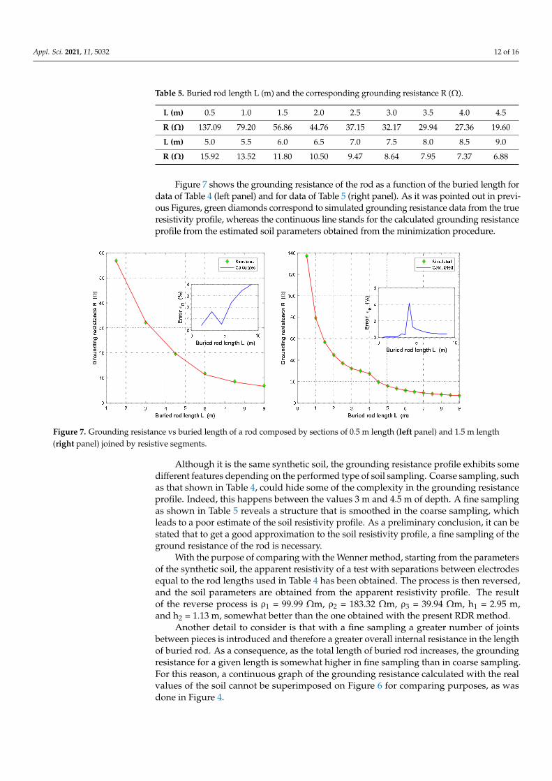
Figure 7 shows the grounding resistance of the rod as a function of the buried length fordata of Table 4 (left panel) and for data of Table 5 (right panel). As it was pointed out in previ-ous Figures, green diamonds correspond to simulated grounding resistance data from the trueresistivity profile, whereas the continuous line stands for the calculated grounding resistanceprofile from the estimated soil parameters obtained from the minimization procedure.

Appl. Sci. 2021, 11, 5032 12 of 16

2.77 m, h2 = 1.33 m. As in the previous examples, values significantly different from the true ones are estimated for the intermediate layer. As mentioned before, this fact is related to the size of the rods, which results in a coarse sampling of the grounding resistance. Refining the sampling by using low-resistive rods 0.5 m length together with the junction segments, the simulated grounding resistance is shown in Table 5. The estimated soil pa-rameters are ρ1 = 99.99 Ωm, ρ2 = 201.32 Ωm, ρ3 = 40.01 Ωm, h1 = 2.99 m, and h2 = 1.02 m which are very close to the real values taken as starting point.

Table 5. Buried rod length L (m) and the corresponding grounding resistance R (Ω).

L(m) 0.5 1.0 1.5 2.0 2.5 3.0 3.5 4.0 4.5 R(Ω) 137.09 79.20 56.86 44.76 37.15 32.17 29.94 27.36 19.60 L(m) 5.0 5.5 6.0 6.5 7.0 7.5 8.0 8.5 9.0 R(Ω) 15.92 13.52 11.80 10.50 9.47 8.64 7.95 7.37 6.88

Figure 7 shows the grounding resistance of the rod as a function of the buried length for data of Table 4 (left panel) and for data of Table 5 (right panel). As it was pointed out in previous Figures, green diamonds correspond to simulated grounding resistance data from the true resistivity profile, whereas the continuous line stands for the calculated grounding resistance profile from the estimated soil parameters obtained from the mini-mization procedure.

Although it is the same synthetic soil, the grounding resistance profile exhibits some different features depending on the performed type of soil sampling. Coarse sampling, such as that shown in Table 4, could hide some of the complexity in the grounding re-sistance profile. Indeed, this happens between the values 3 m and 4.5 m of depth. A fine sampling as shown in Table 5 reveals a structure that is smoothed in the coarse sampling, which leads to a poor estimate of the soil resistivity profile. As a preliminary conclusion, it can be stated that to get a good approximation to the soil resistivity profile, a fine sam-pling of the ground resistance of the rod is necessary.

With the purpose of comparing with the Wenner method, starting from the parame-ters of the synthetic soil, the apparent resistivity of a test with separations between elec-trodes equal to the rod lengths used in Table 4 has been obtained. The process is then reversed, and the soil parameters are obtained from the apparent resistivity profile. The result of the reverse process is ρ1 = 99.99 Ωm, ρ2 = 183.32 Ωm, ρ3 = 39.94 Ωm, h1 = 2.95 m, and h2 = 1.13 m, somewhat better than the one obtained with the present RDR method.

Figure 7. Grounding resistance vs buried length of a rod composed by sections of 0.5 m length (left panel) and 1.5 m length (right panel) joined by resistive segments. Figure 7. Grounding resistance vs buried length of a rod composed by sections of 0.5 m length (left panel) and 1.5 m length(right panel) joined by resistive segments.

Although it is the same synthetic soil, the grounding resistance profile exhibits somedifferent features depending on the performed type of soil sampling. Coarse sampling, suchas that shown in Table 4, could hide some of the complexity in the grounding resistanceprofile. Indeed, this happens between the values 3 m and 4.5 m of depth. A fine samplingas shown in Table 5 reveals a structure that is smoothed in the coarse sampling, whichleads to a poor estimate of the soil resistivity profile. As a preliminary conclusion, it can bestated that to get a good approximation to the soil resistivity profile, a fine sampling of theground resistance of the rod is necessary.

With the purpose of comparing with the Wenner method, starting from the parametersof the synthetic soil, the apparent resistivity of a test with separations between electrodesequal to the rod lengths used in Table 4 has been obtained. The process is then reversed,and the soil parameters are obtained from the apparent resistivity profile. The resultof the reverse process is ρ1 = 99.99 Ωm, ρ2 = 183.32 Ωm, ρ3 = 39.94 Ωm, h1 = 2.95 m,and h2 = 1.13 m, somewhat better than the one obtained with the present RDR method.

Another detail to consider is that with a fine sampling a greater number of jointsbetween pieces is introduced and therefore a greater overall internal resistance in the lengthof buried rod. As a consequence, as the total length of buried rod increases, the groundingresistance for a given length is somewhat higher in fine sampling than in coarse sampling.For this reason, a continuous graph of the grounding resistance calculated with the realvalues of the soil cannot be superimposed on Figure 6 for comparing purposes, as wasdone in Figure 4.

Appl. Sci. 2021, 11, 5032 13 of 16

3.3. Real Examples with Internal Resistance

So far, only synthetic resistivity profiles have been considered in order to test the feasi-bility of the RDR method for recovering the soil structure when real electrodes and practicalprocedures are used. Next, some real cases corresponding to coarse sampling groundingresistance test will be analyzed. The data has been kindly provided by the INGESCO LightingSolutions firm, located in Terrassa, Barcelona (Spain), for academic purposes.

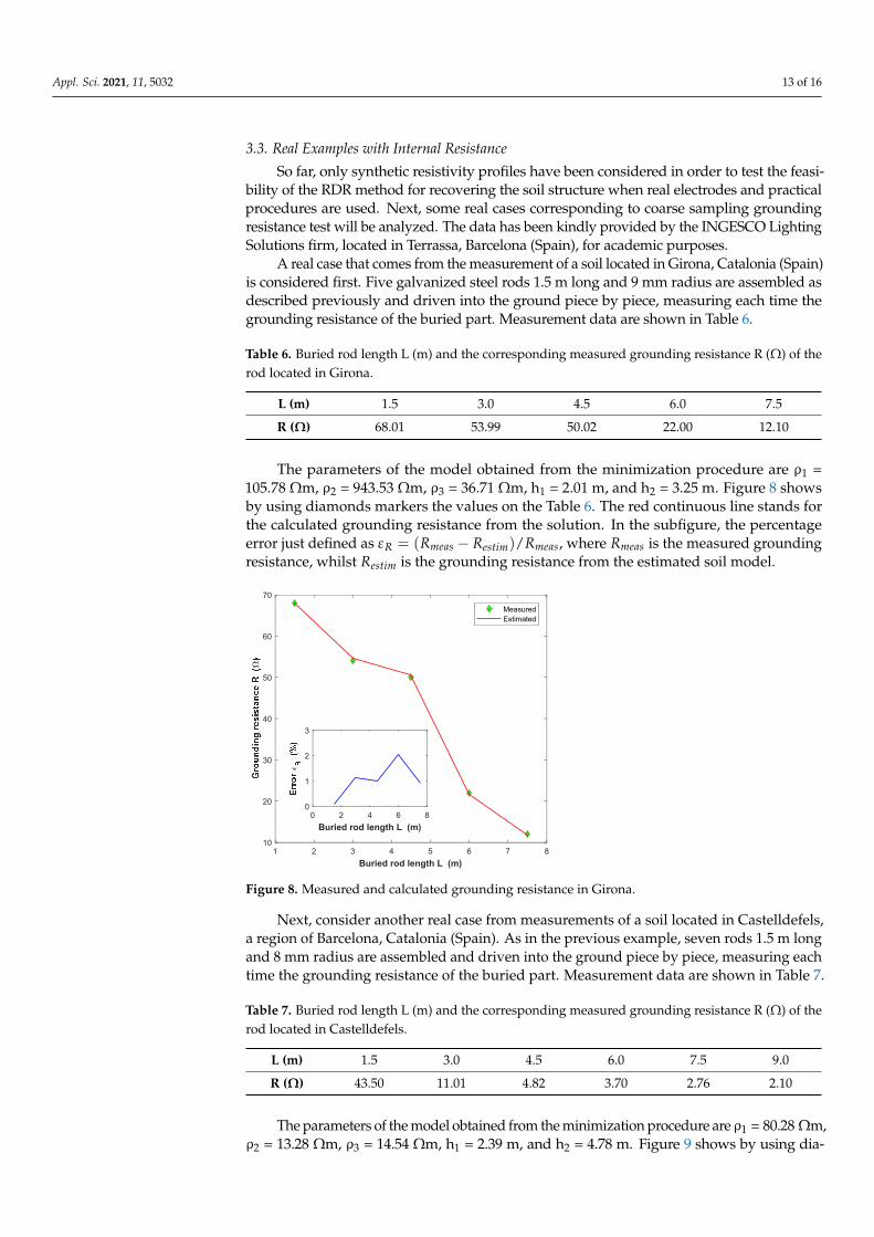
A real case that comes from the measurement of a soil located in Girona, Catalonia (Spain)is considered first. Five galvanized steel rods 1.5 m long and 9 mm radius are assembled asdescribed previously and driven into the ground piece by piece, measuring each time thegrounding resistance of the buried part. Measurement data are shown in Table 6.

Table 6. Buried rod length L (m) and the corresponding measured grounding resistance R (Ω) of therod located in Girona.

L (m) 1.5 3.0 4.5 6.0 7.5

R (Ω) 68.01 53.99 50.02 22.00 12.10

The parameters of the model obtained from the minimization procedure are ρ1 =105.78 Ωm, ρ2 = 943.53 Ωm, ρ3 = 36.71 Ωm, h1 = 2.01 m, and h2 = 3.25 m. Figure 8 showsby using diamonds markers the values on the Table 6. The red continuous line stands forthe calculated grounding resistance from the solution. In the subfigure, the percentageerror just defined as εR = (Rmeas − Restim)/Rmeas, where Rmeas is the measured groundingresistance, whilst Restim is the grounding resistance from the estimated soil model.

Appl. Sci. 2021, 11, 5032 13 of 16

grounding resistance for a given length is somewhat higher in fine sampling than in coarse sampling. For this reason, a continuous graph of the grounding resistance calculated with the real values of the soil cannot be superimposed on Figure 6 for comparing purposes, as was done in Figure 4.

3.3. Real Examples with Internal Resistance So far, only synthetic resistivity profiles have been considered in order to test the

feasibility of the RDR method for recovering the soil structure when real electrodes and practical procedures are used. Next, some real cases corresponding to coarse sampling grounding resistance test will be analyzed. The data has been kindly provided by the IN-GESCO Lighting Solutions firm, located in Terrassa, Barcelona (Spain), for academic pur-poses.

A real case that comes from the measurement of a soil located in Girona, Catalonia (Spain) is considered first. Five galvanized steel rods 1.5 m long and 9 mm radius are assembled as described previously and driven into the ground piece by piece, measuring each time the grounding resistance of the buried part. Measurement data are shown in Table 6.

Table 6. Buried rod length L (m) and the corresponding measured grounding resistance R (Ω) of the rod located in Girona.

L(m) 1.5 3.0 4.5 6.0 7.5 R(Ω) 68.01 53.99 50.02 22.00 12.10

The parameters of the model obtained from the minimization procedure are ρ1 = 105.78 Ωm, ρ2 = 943.53 Ωm, ρ3 = 36.71 Ωm, h1 = 2.01 m, and h2 = 3.25 m. Figure 8 shows by using diamonds markers the values on the Table 6. The red continuous line stands for the calculated grounding resistance from the solution. In the subfigure, the percentage error just defined as ( ) /R meas estim measR R Rε = − , where measR is the measured grounding re-sistance, whilst estimR is the grounding resistance from the estimated soil model.

Figure 8. Measured and calculated grounding resistance in Girona.

Next, consider another real case from measurements of a soil located in Castelldefels, a region of Barcelona, Catalonia (Spain). As in the previous example, seven rods 1.5 m

1 2 3 4 5 6 7 8Buried rod length L (m)

10

20

30

40

50

60

70MeasuredEstimated

0 2 4 6 8Buried rod length L (m)

0

1

2

3

Figure 8. Measured and calculated grounding resistance in Girona.

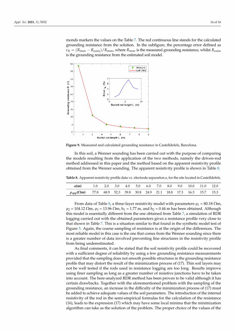
Next, consider another real case from measurements of a soil located in Castelldefels,a region of Barcelona, Catalonia (Spain). As in the previous example, seven rods 1.5 m longand 8 mm radius are assembled and driven into the ground piece by piece, measuring eachtime the grounding resistance of the buried part. Measurement data are shown in Table 7.

Table 7. Buried rod length L (m) and the corresponding measured grounding resistance R (Ω) of therod located in Castelldefels.

L (m) 1.5 3.0 4.5 6.0 7.5 9.0

R (Ω) 43.50 11.01 4.82 3.70 2.76 2.10

The parameters of the model obtained from the minimization procedure are ρ1 = 80.28 Ωm,ρ2 = 13.28 Ωm, ρ3 = 14.54 Ωm, h1 = 2.39 m, and h2 = 4.78 m. Figure 9 shows by using dia-

Appl. Sci. 2021, 11, 5032 14 of 16

monds markers the values on the Table 7. The red continuous line stands for the calculatedgrounding resistance from the solution. In the subfigure, the percentage error defined asεR = (Rmeas − Restim)/Rmeas, where Rmeas is the measured grounding resistance, whilst Restimis the grounding resistance from the estimated soil model.

Appl. Sci. 2021, 11, 5032 14 of 16

long and 8 mm radius are assembled and driven into the ground piece by piece, measur-ing each time the grounding resistance of the buried part. Measurement data are shown in Table 7.

Table 7. Buried rod length L (m) and the corresponding measured grounding resistance R (Ω) of the rod located in Castelldefels.

L(m) 1.5 3.0 4.5 6.0 7.5 9.0 R(Ω) 43.50 11.01 4.82 3.70 2.76 2.10

The parameters of the model obtained from the minimization procedure are ρ1 = 80.28 Ωm, ρ2 = 13.28 Ωm, ρ3 = 14.54 Ωm, h1 = 2.39 m, and h2 = 4.78 m. Figure 9 shows by using diamonds markers the values on the Table 7. The red continuous line stands for the cal-culated grounding resistance from the solution. In the subfigure, the percentage error de-fined as ( ) /R meas estim measR R Rε = − , where measR is the measured grounding resistance, whilst estimR is the grounding resistance from the estimated soil model.

Figure 9. Measured and calculated grounding resistance in Castelldefels, Barcelona.

In this soil, a Wenner sounding has been carried out with the purpose of comparing the models resulting from the application of the two methods, namely the driven-rod method addressed in this paper and the method based on the apparent resistivity profile obtained from the Wenner sounding. The apparent resistivity profile is shown in Table 8.

Table 8. Apparent resistivity profile data vs. electrode separation a, for the site located in Cas-telldefels.

a(m) 1.0 2.0 3.0 4.0 5.0 6.0 7.0 8.0 9.0 10.0 11.0 12.0 ρapp(Ωm) 77.8 68.9 52.3 39.8 30.8 24.9 21.1 18.8 17.3 16.3 15.7 15.3

From data of Table 8, a three-layer resistivity model with parameters ρ1 = 80.18 Ωm, ρ2 = 104.12 Ωm, ρ3 = 13.96 Ωm, h1 = 1.77 m, and h2 = 0.44 m has been obtained. Although this model is essentially different from the one obtained from Table 7, a simulation of RDR logging carried out with the obtained parameters gives a resistance profile very close to that shown in Table 7. This is a situation similar to that found in the synthetic model test of Figure 5. Again, the coarse sampling of resistance is at the origin of the differences. The most reliable model in this case is the one that comes from the Wenner sounding since

Figure 9. Measured and calculated grounding resistance in Castelldefels, Barcelona.

In this soil, a Wenner sounding has been carried out with the purpose of comparingthe models resulting from the application of the two methods, namely the driven-rodmethod addressed in this paper and the method based on the apparent resistivity profileobtained from the Wenner sounding. The apparent resistivity profile is shown in Table 8.

Table 8. Apparent resistivity profile data vs. electrode separation a, for the site located in Castelldefels.

a(m) 1.0 2.0 3.0 4.0 5.0 6.0 7.0 8.0 9.0 10.0 11.0 12.0

ρapp(Ωm) 77.8 68.9 52.3 39.8 30.8 24.9 21.1 18.8 17.3 16.3 15.7 15.3

From data of Table 8, a three-layer resistivity model with parameters ρ1 = 80.18 Ωm,ρ2 = 104.12 Ωm, ρ3 = 13.96 Ωm, h1 = 1.77 m, and h2 = 0.44 m has been obtained. Althoughthis model is essentially different from the one obtained from Table 7, a simulation of RDRlogging carried out with the obtained parameters gives a resistance profile very close tothat shown in Table 7. This is a situation similar to that found in the synthetic model test ofFigure 5. Again, the coarse sampling of resistance is at the origin of the differences. Themost reliable model in this case is the one that comes from the Wenner sounding since thereis a greater number of data involved preventing fine structures in the resistivity profilefrom being underestimated.

As final comments, it can be stated that the soil resistivity profile could be recoveredwith a sufficient degree of reliability by using a few grounding resistance measurementsprovided that the sampling does not smooth possible structures in the grounding resistanceprofile that may distort the result of the minimization process of (17). Thin soil layers maynot be well tested if the rods used in resistance logging are too long. Results improveusing finer sampling as long as a greater number of resistive junctions have to be takeninto account. The here-analyzed RDR method has been proven to be valid although it hascertain drawbacks. Together with the aforementioned problem with the sampling of thegrounding resistance, an increase in the difficulty of the minimization process of (17) mustbe added to achieve adequate values of the soil parameters. The introduction of the internalresistivity of the rod in the semi-empirical formulas for the calculation of the resistance(16), leads to the expression (17) which may have some local minima that the minimizationalgorithm can take as the solution of the problem. The proper choice of the values of the

Appl. Sci. 2021, 11, 5032 15 of 16

parameters that start the minimization process is important. For this reason, it is necessaryto repeat the minimization process with different initial values and analyze the final results.This situation is much less frequent in the method based on apparent resistivity.

4. Conclusions

Assuming a multilayer model for a soil, its parameters can be estimated by means of agrounding resistance logging carried out by means of a vertical rod that is progressivelyintroduced into the soil. As a novelty compared to previous studies, the internal resistanceof the rod is taken into account. Thus, the term Resistive Driven-Rod method is introduced.After establishing a resistance calculation procedure based on semi-analytical expressionsthat include the aforementioned internal resistance of the rod, several application exampleswere considered, from rods without internal resistance in synthetic soils to experiments inreal soils with real rods. The examples discussed show the viability of RDR under certainconditions, which do not represent major problems in the more popular apparent resistivitymethod. Rod resistance sampling should not smooth out possible structures in the groundresistance logging. This problem is not easy to avoid since fixed length pieces of rod areusually available that are assembled and inserted into the ground, measuring the resistancenext. The union between pieces can introduce a contact resistance that must be taken intoaccount. Mainly, the size of the rod pieces determines the resistance sampling. Thesecannot be too small for technical reasons. In addition, the process of searching for the soilresistivity profile by minimizing (17) must be repeated in order to avoid spurious solutions.For coarse sampling, it is possible to find various soil resistivity profiles compatible withRDR sounding values. Only the profile that corresponds to the actual soil can be selectedby finer sampling.

As a final comment, although RDR is a clearly invasive method with the alreadymentioned drawbacks, it has some well-known advantages. Among them stands out amore direct and local estimate of the soil resistivity profile, suitable when there is thepossibility of significant lateral variations in soil resistivity.

Author Contributions: Conceptualization, G.D. and E.F.; methodology, G.D., E.F. and G.A.; software,G.A. and J.M.; validation, G.D. and J.M.; formal analysis, G.D. and E.F.; investigation, G.D., E.F. andG.A.; data curation, J.M.; writing—original draft preparation, G.D., E.F.; writing—review and editing,G.D., E.F., G.A. and J.M. All authors have read and agreed to the published version of the manuscript.

Funding: This research received no external funding.

Institutional Review Board Statement: Not applicable.

Informed Consent Statement: Not applicable.

Data Availability Statement: The data used in this paper are not public but has been kindly providedby the INGESCO Lighting Solutions firm, located in Terrassa, Barcelona (Spain), for academic purposes.

Acknowledgments: The authors would like to thank the Department of Electrical Engineering,Applied Mathematics and Applied Physics of the Escuela Técnica Superior de Ingeniería y DiseñoIndustrial (ETSIDI) at Universidad Politécnica de Madrid (UPM) for their support in undertakingof the research summarized here. Furthermore, the authors appreciate the collaboration with thefirm INGESCO Lightning Solutions at Terrassa, Barcelona (Spain), for the technical support and datatransfer from real cases studied in this work.

Conflicts of Interest: The authors declare no conflict of interest.

References1. Sunde, E.D. Earth Conduction Effects in Transmission Systems; Dover: New York, NY, USA, 1949.2. Wenner, F. A method of measuring earth resistivity. Bull. Bur. Stand. 1916, 12, 469. [CrossRef]3. Zohdy, A.A.R. A new method for the automatic interpretation of Schlumberger and Wenner sounding curves. Geophysics

1989, 54, 245–253. [CrossRef]4. Yang, H.; Yuan, J.; Zong, W. Determination of three-layer earth model from Wenner four-probe test data. IEEE Trans. Magn. 2001,

37, 3684–3687. [CrossRef]

Appl. Sci. 2021, 11, 5032 16 of 16

5. Gupta, P.K.; Niwas, S.; Gaur, V.K. Straightforward inversion of vertical electrical sounding data. Geophysics 1997, 62, 775–785.[CrossRef]

6. Sharma, S.; Verma, G.K. Inversion of Electrical Resistivity Data: A Review. Int. J. Comput. Syst. Eng. 2015, 9, 400–406.7. IEEE Std 80-2000, IEEE Guide for Safety in AC Substation Grounding; IEEE: Piscataway, NJ, USA, 2000.8. Tagg, G.F. Earth Resistances. Pitman: New York, NY, USA, 1964.9. Faleiro, E.; Asensio, G.; Denche, G.; García, D.; Moreno, J. Wenner sounding for apparent resistivity measurements at small

depths using a set of unequal bare electrodes: Selected case studies. Energies 2019, 12, 695. [CrossRef]10. Liu, H. Principles and Applications of Well Logging; Springer Geophysics; Springer: Berlin/Heidelberg, Germany, 2017.11. Li, Y.; Theodoulidis, T.; Tian, G.Y. Magnetic Field-Based Eddy-Current Modeling for Multilayered Specimens. IEEE Trans. Magn.

2007, 43, 4010–4015. [CrossRef]12. Zou, J.; Zeng, R.; He, J.L.; Guo, J.; Gao, Y.Q.; Chen, S.M. Numerical Green’s Function of a Point Current Source in Horizontal

Multilayer Soils by Utilizing the Vector Matrix Pencil Technique. IEEE Trans. Magn. 2004, 40, 730–733. [CrossRef]13. Michalski, K.A.; Mosig, J.R. Efficient computation of Sommerfeld integral tails—Methods and algorithms. J. Electromagn. Waves

Appl. 2016, 30, 281–317. [CrossRef]14. Abramowitz, M.; Stegun, I.A. Handbook of Mathematical Functions; Dover Publications, Inc.: New York, NY, USA, 1972.15. Islam, T.; Chik, Z.; Mustafa, M.M.; Sanusi, H. Estimation of Soil Electrical Properties in a Multilayer Earth Model with Boundary

Element Formulation. Math. Probl. Eng. 2012, 2012, 472457. [CrossRef]16. Gibson, W.C. The Method of Moments in Electromagnetics; Chapman & Hall: London, UK, 2008.17. Otero, A.; Cidras, J.; Del Alamo, J. Frequency-dependent grounding system calculation by means of a conventional nodal analysis

technique. IEEE Trans. Power Deliv. 1999, 14, 873–878. [CrossRef]18. Kuhar, A.; Grcev, L. Contribution to calculating the impedance of grounding electrodes using circuit equivalents. Facta Univ. Ser.

Electron. Energ. 2016, 29, 721–732. [CrossRef]19. Visacro, S.; Soares, A. HEM: A Model for Simulation of Lightning-Related Engineering Problems. IEEE Trans. Power Deliv. 2005,

20, 1206–1208. [CrossRef]