International evidence on stochastic and deterministic monetary neutrality

Banco de Mexico

Documentos de Investigacion

Banco de Mexico

Working Papers

N◦ 2008-04

International Evidence on Stochastic and Deterministic MonetaryNeutrality

Antonio E. Noriega Luis M. SoriaBanco de Mexico, Universidad de Guanajuato Universidad de Guanajuato

Ramon VelazquezUniversidad de Guanajuato

April 2008

La serie de Documentos de Investigacion del Banco de Mexico divulga resultados preliminares detrabajos de investigacion economica realizados en el Banco de Mexico con la finalidad de propiciarel intercambio y debate de ideas. El contenido de los Documentos de Investigacion, ası como lasconclusiones que de ellos se derivan, son responsabilidad exclusiva de los autores y no reflejannecesariamente las del Banco de Mexico.

The Working Papers series of Banco de Mexico disseminates preliminary results of economicresearch conducted at Banco de Mexico in order to promote the exchange and debate of ideas. Theviews and conclusions presented in the Working Papers are exclusively the responsibility of theauthors and do not necessarily reflect those of Banco de Mexico.

Documento de Investigacion Working Paper2008-04 2008-04

International Evidence on Stochastic and Deterministic MonetaryNeutrality*

Antonio E. Noriega† Luis M. Soria‡

Banco de Mexico Universidad de GuanajuatoUniversidad de Guanajuato

Ramon Velazquez§

Universidad de Guanajuato

AbstractWe analyze the issue of the impact of multiple breaks on monetary neutrality results, using

a long annual international data set. We empirically verify whether neutrality propositionsremain addressable (and if so, whether they hold or not), when unit root tests are carriedout allowing for multiple structural breaks in the long-run trend function of the variables. Itis found that conclusions on neutrality are sensitive to the number and location of breaks. Inorder to interpret the evidence for structural breaks, we introduce a notion of deterministicmonetary neutrality, which naturally arises in the absence of permanent stochastic shocksto the variables.Keywords: Deterministic and Stochastic Neutrality and Superneutrality of Money, UnitRoots, Structural Breaks, Resampling Methods.JEL Classification: C15, C32, E51, E52

ResumenEste artıculo analiza el impacto de cambios estructurales multiples sobre resultados de

neutralidad monetaria, utilizando una base de datos internacional. Investigamos empırica-mente si las proposiciones de neutralidad pueden ser verificables (y si lo son, si se mantieneno no), cuando las pruebas de raız unitaria se aplican permitiendo cambios estructuralesmultiples en la funcion de tendencia de largo plazo de las variables. Encontramos que lasconclusiones sobre neutralidad son sensibles al numero de cambios y a su localizacion en lamuestra. Para interpretar la evidencia de cambios estructurales, introducimos una nocionde neutralidad monetaria determinıstica, que surge naturalmente en ausencia de choquesestocasticos permanentes en las variables.Palabras Clave: Neutralidad y super neutralidad monetaria determinıstica y estocastica,Raıces unitarias, Cambios estructurales, Metodos de remuestreo.

*With thanks to Daniel Chiquiar, Manuel Ramos-Francia, Alberto Torres, Mario Alberto Oliva, andparticipants at the XI Meeting of the Reseach Network of Central Banks of the Americas, CEMLA andBanco Central de la Republica Argentina, the Computing in Economics and Finance Conference (Universitatvan Amsterdam), the Seminarios de Economıa at Universidad de Guanajuato and at Banco de Mexico,the Workshop on Computational Econometrics and Statistics at Neuchatel, Switzerland, the Seminars inEconomics at El Colegio de Mexico, and the Latin American Meeting of the Econometric Society.

† Direccion General de Investigacion Economica. Email: [email protected]‡ Escuela de Economıa. Email: Soria [email protected]§ Escuela de Economıa Email: [email protected]

1 Introduction

Several empirical studies demonstrate the prevalence of (infrequent) parameter variation in

the trend function of macroeconomic time series, and analyze the impact of such structural

breaks on unit root testing. The common conclusion is that neglected breaks tend to induce

non rejection of the unit root hypothesis.1 Similar problems could arise when testing relevant

hypotheses such as monetary neutrality. In particular, neglecting breaks could bias the

results of tests of monetary neutrality that rely on the time series properties of money and

income, such as those proposed by Fisher and Seater (1993).

Serletis and Koustas (1998) argue that the issue of whether long-run monetary neutrality

(LRN) results hold under the presence of structural breaks -an issue that has not been

resolved yet in the literature- depends on how big shocks are treated. If they are treated

like any other shock, then there is no need to account for them in interpreting neutrality

results. If, on the other hand, they are regarded as (infrequent) big shocks that need to be

accounted for, then conclusions on neutrality may change, because such shocks may induce

lower orders of integration for output and money. Fisher and Seater (1993) (henceforth, FS)

use the convention that if a variable is stationary around a linear trend then it is treated

as trend-stationary, that is, integrated of order zero. Extending FS’s idea, one can say that

if a variable is stationary around a broken trend then it is also integrated of order zero.

This is precisely the interpretation followed by Serletis and Krause (1996), and Serletis and

Koustas (1998). Under their approach, however, the number of structural breaks allowed in

the deterministic trend function is fixed to one. This selection may not be inconsequential.2

In this paper, we analyze precisely the issue of the impact of multiple breaks on monetary

neutrality results. To the best of our knowledge there is no evidence of the effects of structural

breaks on monetary neutrality tests available in the literature. By allowing for broken trend

functions we uncover the presence of structural breaks which alter (reduce) the order of

integration of money and output, therefore modifying conclusions on LRN and long-run super

neutrality (LRSN). We utilize the same data set as Noriega (2004), i.e., long annual data

on real output and monetary aggregates for Argentina (1884-1996), Australia (1870-1997),

Brazil (1912-1995), Canada (1870-2001), Italy (1870-1997), Mexico (1932-2000), Sweden

(1871-1988), and the UK (1871-2000) (The cases of Denmark and the U.S are not analyzed

1Empirical examples with macro time series can be found in Perron (1989, 1992, 1997), Lumsdaine andPapell (1997), Ohara (1999), Mehl (2000), Noriega and De Alba (2001), and Gil-Alana (2002); Perron andVogelsang (1992), Culver and Papell (1995), and Aggarwal et.al. (2000) for real exchange rates; Raj (1992)and Zelhorst and Haan (1995), for real output; Clemente, et. al. (1998) for interest rates, among others.

2In a recent paper, Arestis and Biefang-Frisancho Mariscal (1999) conclude that ”...unit root tests thatdo not account sufficiently for the presence of structural breaks are misspecified and suggest excessive per-sistence”(p.155). See also Perron (2003).

1

in this paper, since evidence in Noriega (2004) suggests that both money and output are

integrated of order zero).

In particular, we empirically verify whether the monetary neutrality propositions remain

addressable (and if so, whether they hold or not), when unit root tests are carried out allowing

for (possibly) multiple structural breaks in the long-run trend function of the variables. It

is found that conclusions on monetary neutrality are sensitive not only to whether there is

a break or not, but also to the number and location of breaks.

Our ultimate finding is that neglected deterministic breaks appear to induce over-rejections

of the LRN hypothesis. To motivate the issue of broken trends and monetary neutrality, con-

sider the case of the U.K. Results in Serletis and Koustas (1998) and Noriega (2004), both

based on the FS methodology, indicate that LRN does not hold for M4. This implies that a

permanent stochastic shock to the level of money has a long lasting real effect on UK output.

Now consider the graphs of real output and money in Figure 1, which indicate the presence

of one structural break in output (1918) and two structural breaks in money (1939, 1970)3.

As can be seen, even though M4 underwent two breaks, one in level and another one in

level and slope of trend, real output did not register any major change in its long-run trend

function, from 1919 to 2000; it actually fluctuated in a stationary fashion for over 80 years.

Figure 1UK real output (left) and money (M4, right), 1871-2000

2.5

3.0

3.5

4.0

4.5

5.0

5.5

1880 1900 1920 1940 1960 1980 20000

2

4

6

8

10

1880 1900 1920 1940 1960 1980 2000

Based on this evidence, in sharp contradiction with recent research in the area, it could

be argued that money has been neutral in the UK for most of the twentieth century. This

is a case of rejection of the LRN hypothesis due to neglected breaks. Cases like this point

to an heuristic notion of deterministic neutrality, to be introduced below.

We use as our starting point the results recently obtained in Noriega (2004) regarding

3Details on how to estimate the number and location of breaks will be given below.

2

the order of integration of money and output for the data set described above4. After a brief

review of the FS methodology, we analyze in section 2, the behaviour of these orders of inte-

gration under different trend specifications, allowing for an increasing number of structural

breaks in the long-run trend function under the alternative hypothesis. Note that under

broken trend-stationary models, permanent changes are deterministic, as opposed to sto-

chastic.5 This allows the possibility of investigating any potential relationship between the

estimated break dates and historic events. Section 3 offers an alternative heuristic interpre-

tation of ’deterministic neutrality’ based on the presence of these permanent deterministic

shocks. It reports the empirical results under both the traditional stochastic interpretation

based on FS, and the deterministic one. Section 4 concludes.

2 Econometric Methodology

2.1 The FS tests of LRN and LRSN

Economists care about long-run monetary neutrality (LRN) because most theoretical models

of money predict that money is neutral in the long-run; that is, the real effects of an unan-

ticipated, permanent change in the level of money, tend to disappear as time elapses. They

also care about LRN because LRN is often used as an identification assumption (i.e. the

large literature using Blanchard-Quah (1989) decompositions). On the other hand, the case

for monetary superneutrality has limited theoretical support6. As summarized by Bullard

(1999), ”if monetary growth causes inflation, and inflation has distortionary effects, then

long-run monetary superneutrality should not hold in the data. On the contrary, a per-

manent shock to the rate of monetary growth should have some long-run effect on the real

economy; why else should we worry about it?” (p.59).

Empirical results based on the reduced-form tests of Long Run Neutrality (LRN) and

Long Run Superneutrality (LRSN), derived by FS, depend on the order of integration of

both real output and the money aggregates. A number of recent papers examine the validity

of these key macro propositions using long annual data and the reduced form tests of FS7.

4Noriega (2004) determined the order of integration of money and output by estimating the number ofunit roots present in the data, under the asymptotically consistent sequential procedure of Pantula (1989),using the unit root tests developed by Ng and Perron (2001).

5Our econometric methodology borrows from Ng and Perron (1995), Bai and Perron (1998a, b), andNoriega and de Alba (2001).

6In the literature on monetary growth theory, there are very few available models which embody someform of monetary superneutrality. See for instance, Sidrauski (1967), Hayakawa (1995) and Faria (2001).

7Bae and Jensen (1999) examine these propositions by extending FS long-run neutrality requirements tolong-memory processes. An alternative econometric perspective of LRN and LRSN is presented in King andWatson (1997).

3

In this literature, the orders of integration are identified through the application of common

used test, as the Augmented Dickey-Fuller, ADF, of Said and Dickey (1984), the Z tests

of Phillips-Perron (1988), and the stationarity KPSS tests of Kwiatkowski, et. al. (1992),

to real output and the money aggregates. For instance, LRN finds empirical support in

the studies of Boschen and Otrok (1994, US data), Haug and Lucas (1997, Canadian data),

Serletis and Krause (1996, international data set), Wallace (1999, Mexican data), and Bae

and Ratti (2000 Brazilian and Argentinean data). Utilizing the more powerful tests of Ng

and Perron (2001), Noriega (2004, international data set) finds weaker support for LRN.

Even though the paper’s objective is not to derive conclusions on monetary neutrality

based on the FS methodology, we do apply it and use the results as a benchmark against

which we compare results based on the methodology put forward in the next subsection, for

which neutrality testing also depends on permanent shocks, but of a deterministic nature.

This subsection briefly presents the main ingredients of the FS methodology. They show

that LRN and LRSN can be tested through the significance of the slope parameters bk in

the following long-horizon (OLS) regression:

"kX

j=0

∆hyiyt−j

#= ak + bk

"kX

j=0

∆hmimt−j

#+ εkt, (1)

where y and m stand for real output and (exogenous) money; ∆ represents the difference

operator (∆jyt = yt − yt−j), hyi stands for the order of integration of y (i.e. hyi = 1 meansthat y is integrated of order one, or y ∼ I(1)), and ε is a mean zero uncorrelated random

variable. Theoretically, limk→∞ bk ≡ b, gives an estimate of the long-run derivative (LRD)

of real output with respect to a permanent stochastic exogenous shock in both the level of

money (denoted LRDN), and the growth rate (trend) of money (denoted LRDSN).

FS show that, in order to interpret neutrality results, the order of integration of output

and money should obey certain restrictions. For instance, the order of integration of money

should be at least equal to one (hmi ≥ 1) for LRN to make sense, otherwise there are nostochastic permanent changes in money that can affect real output. Table 1 summarizes

values of the LRD under different possibilities on the order of integration of the variables.

According to the table, when hmi ≥ hyi + 1 ≥ 1 the long-run derivative is zero, providingdirect evidence of neutrality. When hmi = hyi = 1, LRN is testable through b. In this

case, LRDN measures whether the permanent movements in output are associated with

permanent stochastic movements in the level of money. If for instance b is significantly

different from zero, then LRN does not hold.

4

Table 1The LRD and the Order of Integration of Money and Output

LRDN LRDSN

hyi hmi = 0 hmi = 1 hmi = 2 hmi = 0 hmi = 1 hmi = 20 undefined ≡ 0 ≡ 0 undefined undefined ≡ 01 undefined b ≡ 0 undefined undefined b

Source: Adapted from Fisher and Seater (1993).

Superneutrality, however, is not addressable when there are no permanent stochastic

changes in the growth rate of money. In other words, superneutrality requires hmi ≥ 2.

When hmi = 2 and hyi = 0, LRDN = LRDSN = 0, i.e., both LRN and LRSN hold,

since one cannot associate permanent shocks to the growth rate of money to nonexistent

permanent changes in output (further discussion of several cases of interest can be found in

FS). Therefore, proper determination of the orders of integration of y and m is crucial in

assessing LRN and LRSN of money.

Finally, it is important to mention that since the neutrality tests of FS are based on how

changes in the level of money are ultimately related to changes in output, cointegration is

neither necessary nor sufficient for long-run neutrality.8

2.2 Unit roots and structural breaks in money and output

Fisher and Seater‘s tests of monetary neutrality rely on the presence of stochastic permanent

changes in money and output. If there are no such changes in either variable, then LRN is

unaddressable (the LRDN is undefined). On the other hand if there is a stochastic permanent

change in the level of money, while output follows a stationary process, then LRN holds by

definition (since LRDN = 0).

The presence of permanent stochastic changes in money and output, as indeed in many

other macro variables depends, however, on the way the trend function is treated, i.e., the

modelling of the long-run. The most common approaches in the literature include linear

trends (Nelson and Plosser (1982)), broken trends (Perron (1989, 1997)), polynomial trends

(Schmidt and Phillips (1992)), the Hodrick-Prescott filter (Hodrick and Prescott (1997),

Cogley and Nason (1995)), and smooth transition trend models (Leybourne, et. al. (1998),

Sollis, et. al. (1999)).9 Among these, models allowing for structural breaks (broken trend

models) have become very popular in the literature, both theoretical and applied (Lanne,

8See Fisher and Seater (1993) p. 414-15 for details.9See also Pollock (2001) for the analysis of three different approaches to the estimation of econometric

trends.

5

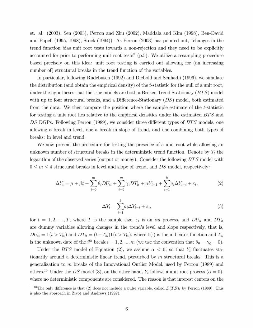
et. al. (2003), Sen (2003), Perron and Zhu (2002), Maddala and Kim (1998), Ben-David

and Papell (1995, 1998), Stock (1994)). As Perron (2003) has pointed out, ”changes in the

trend function bias unit root tests towards a non-rejection and they need to be explicitly

accounted for prior to performing unit root tests” (p.5). We utilize a resampling procedure

based precisely on this idea: unit root testing is carried out allowing for (an increasing

number of) structural breaks in the trend function of the variables.

In particular, following Rudebusch (1992) and Diebold and Senhadji (1996), we simulate

the distribution (and obtain the empirical density) of the t-statistic for the null of a unit root,

under the hypotheses that the true models are both a Broken Trend Stationary (BTS)model

with up to four structural breaks, and a Difference-Stationary (DS) model, both estimated

from the data. We then compare the position where the sample estimate of the t-statistic

for testing a unit root lies relative to the empirical densities under the estimated BTS and

DS DGPs. Following Perron (1989), we consider three different types of BTS models, one

allowing a break in level, one a break in slope of trend, and one combining both types of

breaks: in level and trend.

We now present the procedure for testing the presence of a unit root while allowing an

unknown number of structural breaks in the deterministic trend function. Denote by Yt the

logarithm of the observed series (output or money). Consider the following BTS model with

0 ≤ m ≤ 4 structural breaks in level and slope of trend, and DS model, respectively:

∆Yt = µ+ βt+mXi=0

θiDUit +mXi=0

γiDTit + αYt−1 +kXi=1

ai∆Yt−i + εt, (2)

∆Yt =kXi=1

ai∆Yt−i + εt, (3)

for t = 1, 2, . . . , T , where T is the sample size, εt is an iid process, and DUit and DTit

are dummy variables allowing changes in the trend’s level and slope respectively, that is,

DUit = 1(t > Tbi) and DTit = (t−Tbi)1(t > Tbi), where 1(·) is the indicator function and Tbiis the unknown date of the ith break i = 1, 2, ...,m (we use the convention that θ0 = γ0 = 0).

Under the BTS model of Equation (2), we assume α < 0, so that Yt fluctuates sta-

tionarily around a deterministic linear trend, perturbed by m structural breaks. This is a

generalization to m breaks of the Innovational Outlier Model, used by Perron (1989) and

others.10 Under the DS model (3), on the other hand, Yt follows a unit root process (α = 0),

where no deterministic components are considered. The reason is that interest centers on the

10The only difference is that (2) does not include a pulse variable, called D(TB)t by Perron (1989). Thisis also the approach in Zivot and Andrews (1992).

6

AR parameter and its associated t-statistic estimated from (2), both of which are invariant

with respect to the parameters µ, β, θi, γi, for any sample size11.

Note that the location (Tbi), type (level, trend, or level and trend), and number (m) of

breaks, as well as the AR order (k) in the above equations are unknown. We proceed as

follows:

1. For the no breaks case (m = 0) one simply runs an ADF test for the presence of a unit root

by estimating (2) with an arbitrary maximum value for k, labeled kmax (see for instance

Ng and Perron (1995)), and reducing the AR order by one as in step 3 below (but ignoring

the use of the AIC).

2. For each value of 1 ≤ m ≤ 4, start with a kmax and estimate (2) by OLS the 3m BTS

models, and chose the location of break(s) from the minimum of the sequence of residual

sum of squares, computed over the m-dimensional grid of combinations of m breaks (as in

Bai and Perron (1998b)):

(bTb1, ..., bTbm) = argminTb1 ,...,Tbm

RSS(Tb1, ..., Tbm),

where the minimization is taken over all partitions Tb1, ..., Tbm such that Tbi − Tbi−1 ≥ h.

This criterion is called minRSS, and it implies simultaneous determination of location for

m breaks via a global search. The partitions of T in m+ 1 segments obey:

k + 1 + h ≤ Tb1 ≤ T −mh

Tb1 + h ≤ Tb2 ≤ T − (m− 1)h...

Tbm−1 + h ≤ Tbm ≤ T − h,

where h represents the smallest possible size for a segment.12

3. The Akaike Information Criterion (AIC) is then calculated for each of these 3m regres-

sions. If the coefficient on the kmaxth lag is not significant for the model which yields the

smallest AIC, then estimate (2) as in step 2, but with kmax−1 lags of the differenced de-pendent variable. Again, compute the AIC for the 3m regressions corresponding to the newly

estimated break dates. Continuing in this fashion, we select the combination ’model type/lag

length’ which corresponds to the model which yields the smallest value of the AIC (amongst

11See for example Perron (1989, p.1393).12This representation for h is based on the dynamic programming algorithm introduced by Bai and Perron

(1998b) to obtain global minimizers of the RSS. In empirical applications below, we set h = 6. Results arerobust to various other choices of h.

7

the 3m models) and a corresponding significant lag (called k), using a two-sided 10% test

based on the asymptotic normal distribution.13

To discriminate between DS and BTS for the cases 1 ≤ m ≤ 4, we simulate the dis-tribution of the t-statistic for the null hypothesis of a unit root (α = 0 in (2)), called bτ ,under the hypotheses that the true models are the BTS models (2) (following steps 1-3) and

the DS model (3), both estimated from the data.14. That is, under the BTS (DS) model

we use the estimated parameters from (2)((3)), and the first k + 1 observations as initial

conditions (∆Y2, ..., ∆Yk+1) to generate 10,000 samples of ∆Yt, t = 2, ..., T, with randomly

selected residuals (with replacement) from the estimated BTS (DS) model. For each gen-

erated sample, regression equation (2) is run and the corresponding 10,000 values of bτ areused to construct the empirical density function of this statistic under the BTS (DS) model,

labeled fBTSm(bτ), m = 0, ..., 4 (fDS(bτ)).15We then obtain the position where the sample estimate of the t-statistic for testing a

unit root (∧τT ) from the estimation of equation (2), lies relative to the empirical (simulated)

densities, for each value of m. These positions are calculated as the probability mass to the

left of∧τT , denoted pBTSm ≡ Pr[bτ ≤ bτT | fBTSm(bτ)] and pDS ≡ Pr[bτ ≤ bτT | fDS(bτ)]. A value

of pDS > 0.10 would indicate that there is not enough evidence in the data against the DS

specification. We conclude in favour of a BTS specification with m structural breaks when

pDS ≤ 0.10 and 0.10 < pBTSm < 0.90.

We use in this section the above discussed convention that if a variable is stationary

around a broken trend then it is integrated of order zero. We discuss below the implication

of such convention. Results are given in Table A1 of the appendix. The first column indicates

the number of breaks allowed in the trend function, m. The second column refers to the

estimated lag length, k. In the empirical applications kmax is set at 5. The next columns

report the estimated break dates. The type of break allowed in the trend function is reported

in parenthesis. Column labeled AC reports the p−values for the Lagrange Multiplier test ofthe null hypothesis that the disturbances are serially uncorrelated against the alternative that

they are autocorrelated of order one. The next column reports the value of the t−statisticfor testing the null hypothesis of a unit root, estimated from equation (2). The probability

mass to the left of this estimate, under each of the simulated DS and BTS specifications, is

presented in the last two columns of the table.

13Note that if there are no significant lags, then k = 0, which implies an AR(1) model for equation (2).If this is the case, the selection of the model follows simply from the lowest value of the AIC. The sameapproach is applied in Noriega and de Alba (2001).14A similar apprach is used by Kuo and Mikkola (1999) for the US/UK real exchange rate series.15The 10,000 fitted regressions utilize the estimated value of k, under the BTS (DS) model. All calcula-

tions were carried out in GAUSS.

8

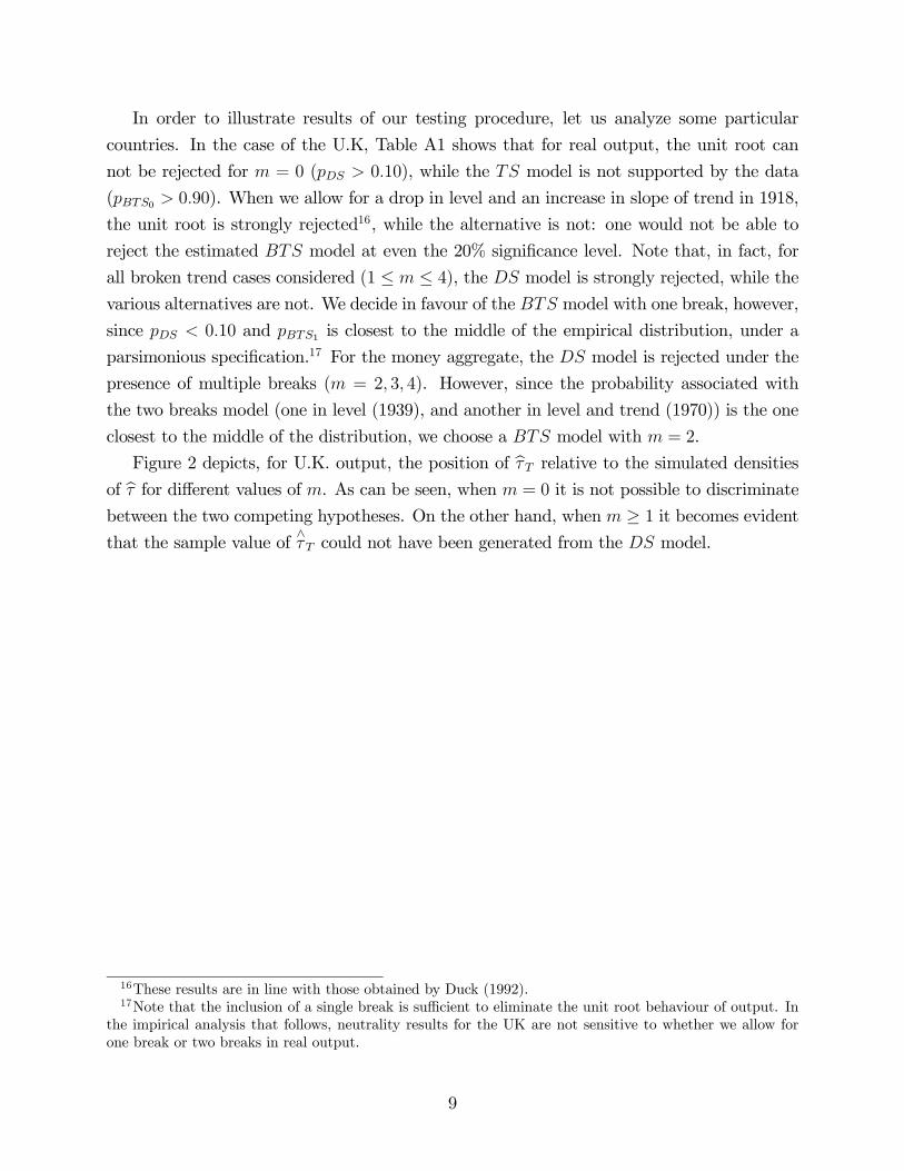
In order to illustrate results of our testing procedure, let us analyze some particular

countries. In the case of the U.K, Table A1 shows that for real output, the unit root can

not be rejected for m = 0 (pDS > 0.10), while the TS model is not supported by the data

(pBTS0 > 0.90). When we allow for a drop in level and an increase in slope of trend in 1918,

the unit root is strongly rejected16, while the alternative is not: one would not be able to

reject the estimated BTS model at even the 20% significance level. Note that, in fact, for

all broken trend cases considered (1 ≤ m ≤ 4), the DS model is strongly rejected, while the

various alternatives are not. We decide in favour of the BTS model with one break, however,

since pDS < 0.10 and pBTS1 is closest to the middle of the empirical distribution, under a

parsimonious specification.17 For the money aggregate, the DS model is rejected under the

presence of multiple breaks (m = 2, 3, 4). However, since the probability associated with

the two breaks model (one in level (1939), and another in level and trend (1970)) is the one

closest to the middle of the distribution, we choose a BTS model with m = 2.

Figure 2 depicts, for U.K. output, the position of bτT relative to the simulated densitiesof bτ for different values of m. As can be seen, when m = 0 it is not possible to discriminate

between the two competing hypotheses. On the other hand, when m ≥ 1 it becomes evidentthat the sample value of

∧τT could not have been generated from the DS model.

16These results are in line with those obtained by Duck (1992).17Note that the inclusion of a single break is sufficient to eliminate the unit root behaviour of output. In

the impirical analysis that follows, neutrality results for the UK are not sensitive to whether we allow forone break or two breaks in real output.

9

Figure 2Empirical Densities of Tao for DS and TS models for United Kingdom Real Output

No breaks case, m=0 One break case, m=1

pBTS0=.933; pDS=.742 pBTS1=.764; pDS=.000

Two breaks case, m=2 Three break case, m=3

pBTS2=.763; pDS=.000 pBTS3=.791; pDS=.000

Four breaks case, m=4

pBTS4=.839; pDS=.000

Figure 3 shows graphs of UK output and money, together with their corresponding fitted

broken trends.

10

Figure 3United Kingdom

Y, I(0) + 1 break : M4, I(0) + 2 breaks:

1918 (LT) 1939(L), 1970 (LT)

2.5

3.0

3.5

4.0

4.5

5.0

5.5

1880 1900 1920 1940 1960 1980 20000

2

4

6

8

10

1880 1900 1920 1940 1960 1980 2000

Note: L stand for Level break, and LT stand for Level and Trend break.

A different picture arises for the case of Argentina. For real output, the DS model is

rejected at the five percent level for all broken trend specifications, while under the BTS

model, the probability closest to the middle of the distribution corresponds to the case of

3 structural breaks. For M2, the probabilities indicate that a stochastic permanent change

cannot be rejected. In fact, for the cases m = 1, 2, the rejection of the DS model is towards

an explosive root, i.e., on the right tail of the empirical distribution. The values of the AR

parameter for these cases are bα = 1.07, 1.08, respectively. For the other two Latin Americaneconomies, Brazil andMexico, the picture is similar: after allowing for breaks, money remains

stochastically nonstationary, while output becomes a broken trend stationary process.18

For Australia output, the DS model can be rejected for 2 ≤ m ≤ 4. However, it is onlyfor m = 3 that the alternative is not rejected (and is closer to the middle of the empirical

distribution). Similar conclusions are reached for the money aggregate. Canadian money

clearly rejects a unit root against a BTS model with one break in level in 1920. For Sweden,

real output and money can be represented by a BTS model with m = 3.

The left-side portion of Table 2 summarizes the empirical results. The countries in the

sample have been grouped according to the effect of breaks on the order of integration of the

variables. The first group includes Australia, Canada, Sweden, and the U.K. For this group,

18In the case of Brazilian output, the DS model is rejected form > 0, and the various BTS alternatives arenot. The combination of probability values corresponding to m = 4 allows clear cut discrimination amongmodels. Similar arguments apply to Mexico output with m = 3. For Brazilian money, when 2 ≤ m ≤ 4,pDS < 0.10, implying rejection of DS. However, the corresponding BTS models are not supported either,since pBTSm > 0.90. Similar arguments apply to Mexican M1 for m = 4. In these cases, we do not concludein favour of a BTS model, since the data also rejects the various alternative hypotheses.

11

the inclusion of breaks has reduced the order of integration of both money and output (with

the exception of Canadian output, which was already known to be I(0) without breaks).

A second group comprises Latin American countries, Argentina, Brazil, and Mexico, for

which real output seems to follow a broken trend stationary model, while money remains

stochastically nonstationary. Finally, for Italy the inclusion of breaks in the trend function

does not alter the order of integration for money and output, already established by Noriega

(2004) as I(1). Hence, the inclusion of breaks has affected the order of integration of 10

series, and, as we show below, will also affect LRN conclusions.

Table 2Summary of Results

Order of Integration LRN LRSN

Country Seriesm = 0∗ m > 0 m=0* m > 0 m=0* m > 0

S D S D

Australia Y I(1) I(0)+3b

M2 I(1) I(0)+2b F NA H NA NA H

Canada Y I(0) I(0)

M2 I(1) I(0)+1b HD NA H NA NA NA

Sweden Y I(1) I(0)+3b

M2 I(1) I(0)+3b H NA - NA NA -

UK Y I(1) I(0)+1b

M4 I(1) I(0)+2b F NA H NA NA H

Argentina Y I(1) I(0)+3b

M2 I(1) I(1) F HD NA NA NA NA

Brazil Y I(1) I(0)+4

M2 I(2) I(2) HD HD NA F HD NA

Mexico Y I(1) I(0)+3b

M1 I(1) I(1) F HD NA NA NA NA

Italy Y I(1) I(1)

M2 I(1) I(1) F - NA NA NA NA

S, D stands for Stochastic and Deterministic respectively.

F, H, HD and NA stands for Fails, Holds, Holds by Definition and Not Addressable, respectively.∗These results are taken from Noriega (2004).

12

3 Stochastic and Deterministic Neutrality

The effect of structural breaks on the order of integration of money and output poses an

interesting question about the testing for monetary neutrality: ¿Should we derive conclusions

on LRN based only on the stochastic version of the FS test? In order to interpret the evidence

for structural breaks presented above, we utilize here an heuristic notion of deterministic

monetary neutrality, which naturally arises in the absence of permanent stochastic shocks

to the variables.

Based on results in the previous section, we present in the right-side portion of Table

2 conclusions on LRN and LRSN. The columns under the headings LRN and LRSN show

whether the neutrality propositions hold (H), fail (F), or are not addressable (NA). Results

are reported for the cases of no breaks (m = 0), and up to 4 breaks (m > 0). When allowing

for breaks, we offer two distinct interpretations: one based on the stochastic (S) version of

neutrality tests (FS)19, and one based on a deterministic (D) version.

Take for instance the U.K. If breaks are not allowed, the FS test indicates that (stochas-

tic) neutrality fails (see Noriega (2004) for details). Allowing for breaks, both variables are

found to follow a stationary process around a broken trend, which means that (stochastic)

LRN is not addressable, since there are no stochastic permanent changes in the variables.

However, under a deterministic interpretation, some form on LRN seems to hold. According

to our results, the long-run behaviour of U.K. output is well characterized as a linear trend,

perturbed by a single break in 1918. On the other hand, U.K. money underwent two struc-

tural breaks, one in level (1938), and the other in level and trend (1970). Note that these

two breaks had no effect on the long-run behaviour of output, which was found to follow

a linear trend from 1918 onwards (see Figure 3). We say that money is deterministically

neutral (DN) for the U.K. since output fluctuates in a stationary fashion around a linear

trend with no breaks from 1918 to 2000. Furthermore, since the 1970 money-break was in

level and trend, we say that U.K. money is also deterministically superneutral (DSN), at

least over a horizon of 30 years.

Similarly, for Australia we conclude that money is DSN (for over 50 years), since the

trend of output remained unaltered, after the occurrence of two monetary breaks in level

and slope of trend (see Figure 4).

19Serletis and Krause (1996) and Serletis and Koustas (1998) utilize this interpretation when analyzingtheir empirical findings. Note that under the stochastic interpretation, we assume, as in previous studies, theexogeneity of money. For a multivariate approach that allows to examine the effects of long-run monetaryendogeneity on reduced-form tests of neutrality see Boschen and Mills (1995).

13

Figure 4Australia

Y, I(0) + 3 breaks M2, I(0) + 2 breaks

1891 (L), 1914 (L), 1928 (L) 1941 (LT), 1971 (LT)

1

2

3

4

5

6

1880 1900 1920 1940 1960 19802

4

6

8

10

12

1880 1900 1920 1940 1960 1980

For Canada, a deterministic interpretation of LRN can also be applied, since the drop

in level of money in 1920 had no effect on the long-run trend of output, which fluctuated

stationarily around a linear trend for over 80 years after the (permanent) monetary break

(see Figure 5).

Figure 5Canada

Y, I(0) M2, I(0) + 1break:

1918 (L)

0

1

2

3

4

5

6

1880 1900 1920 1940 1960 1980 20002

4

6

8

10

12

14

1880 1900 1920 1940 1960 1980 2000

Therefore, for three countries in this first group, the presence of deterministic changes

in the trend function of the variables would lead to the (preliminary) conclusion that (sto-

chastic) LRN is not addressable. Under the deterministic interpretation, on the other hand,

LRN seems to hold for Australia, Canada, and the U.K.

In the case of Sweden, on the other hand, the heuristic notion of deterministic neutrality

cannot be applied, since output experienced structural breaks in its

14

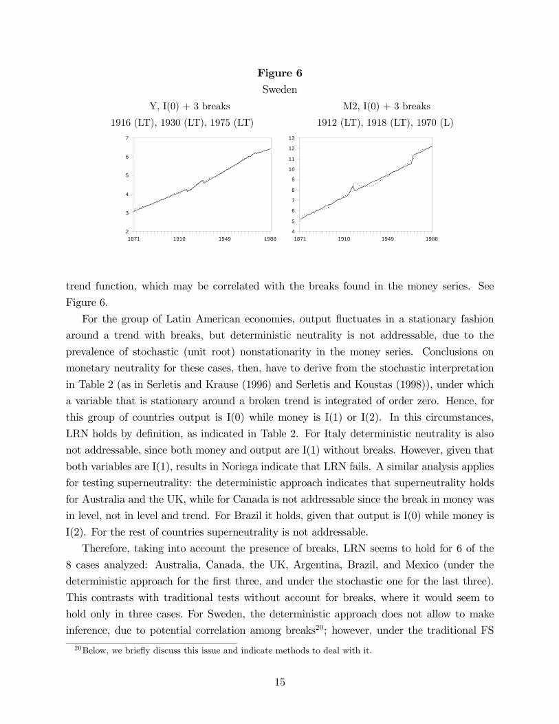
Figure 6Sweden

Y, I(0) + 3 breaks M2, I(0) + 3 breaks

1916 (LT), 1930 (LT), 1975 (LT) 1912 (LT), 1918 (LT), 1970 (L)

2

3

4

5

6

7

1871 1910 1949 19884

5

6

7

8

9

10

11

12

13

1871 1910 1949 1988

trend function, which may be correlated with the breaks found in the money series. See

Figure 6.

For the group of Latin American economies, output fluctuates in a stationary fashion

around a trend with breaks, but deterministic neutrality is not addressable, due to the

prevalence of stochastic (unit root) nonstationarity in the money series. Conclusions on

monetary neutrality for these cases, then, have to derive from the stochastic interpretation

in Table 2 (as in Serletis and Krause (1996) and Serletis and Koustas (1998)), under which

a variable that is stationary around a broken trend is integrated of order zero. Hence, for

this group of countries output is I(0) while money is I(1) or I(2). In this circumstances,

LRN holds by definition, as indicated in Table 2. For Italy deterministic neutrality is also

not addressable, since both money and output are I(1) without breaks. However, given that

both variables are I(1), results in Noriega indicate that LRN fails. A similar analysis applies

for testing superneutrality: the deterministic approach indicates that superneutrality holds

for Australia and the UK, while for Canada is not addressable since the break in money was

in level, not in level and trend. For Brazil it holds, given that output is I(0) while money is

I(2). For the rest of countries superneutrality is not addressable.

Therefore, taking into account the presence of breaks, LRN seems to hold for 6 of the

8 cases analyzed: Australia, Canada, the UK, Argentina, Brazil, and Mexico (under the

deterministic approach for the first three, and under the stochastic one for the last three).

This contrasts with traditional tests without account for breaks, where it would seem to

hold only in three cases. For Sweden, the deterministic approach does not allow to make

inference, due to potential correlation among breaks20; however, under the traditional FS

20Below, we briefly discuss this issue and indicate methods to deal with it.

15

approach, LRN holds for Sweden. Italy seems to be the only country for which LRN fails.

Results for Australia, Canada, the UK, Argentina, and Brazil coincide with results in

Serletis and Krause (1996), Olekalns (1996), Haug and Lucas (1997) and Bae and Ratti

(2000). In this respect it can be argued that neutrality holds under both stochastic and

deterministic permanent shocks. Our results support those of Noriega (2004) only for the

cases where LRN holds: Canada and Brazil. Regarding superneutrality, results for Canada,

Argentina, Mexico and Italy support those of Noriega (2004): LRSN is not addressable. In

contrast to Noriega (2004), our results indicate that superneutrality does hold for Australia

and the UK, once allowance is made for breaks in the trend function.

As noted in section 2.1, under the FS methodology, the order of integration of money

should be equal or greater than one, so that the LRD is defined. On the other hand, the

order of integration of output is not restricted. The only requirement is that hyi ≤ hmi(the order of integration of output can not be greater than that of money). Under the

deterministic interpretation the restrictions are different. Under our approach, one canassociate permanent shocks to the growth rate of money to nonexistent permanent changes

in output. In addition, the identifying restriction of exogenous changes in money is not

required under our approach. We summarize the restrictions needed for a deterministic

interpretation of our empirical results in Table 3.

Table 3Restrictions on hmi and hyi DN Cases

1)hmi : 1 & 0 + breaks

hyi : 1 & 0 + breaksTestable

Australia, Sweden,

UK

2)hmi : 1 & 0 + breaks

hyi : 0→ 0HD Canada

3)hmi : 1→ 1

hyi : 1 & 0 + breaksNA Argentina, Brazil, Mexico

4)hmi : 1→ 1

hyi : 1→ 1NA Italy

The symbols& and→ indicate that the order of integration of the variable has reduced, and maintained,

respectively, after allowing for structural breaks in the trend function.

In case 1), money and output should be stationary around a broken trend for long run

deterministic neutrality (DN) to be testable. We propose two ways for testing DN. One

16

is based on the heuristic analysis of precedence used above: if after a break in m there

are no breaks in y, then we conclude that money is deterministically neutral, if the break

is in level of money, or superneutral if the break is in slope of trend, as in the cases of

Australia and the U.K. The second one suites the case of Sweden, which can be analyzed

using the recently developed theory of co-breaking, introduced in Hendry and Mizon (1998),

Clements and Hendry (1999, chapter 9), and recently advanced and summarized by Hendry

and Massmann (2007), or the techniques for testing for common features (Engle and Kozicki

(1993), Vogelsang and Franses (2001)). The reduced rank technique developed by Krolzig

and Toro (2000) yields information on how breaks are related through economic variables

and across time. The application of these techniques is out of the scope of this paper, and

will be addressed in future research.

For deterministic neutrality to hold by definition, (case 2), both variables should be

stationary, but money around a trend with breaks, as in the case of Canada. Finally, DN

and DSN are not addressable (cases 3 and 4), when at least one of the variables contains a

unit root, as in the cases of Argentina, Brazil, Mexico, and Italy.

4 Concluding Remarks

This paper empirically documents the impact of (endogenously determined) changes in the

long-run trend of money and real output, on the Fisher and Seater (1993) tests of LRN

and LRSN, using a long annual international data set. We present evidence on the inability

to reject plausible broken-trend stationary models that exhibit transitory dynamics around

a long-run deterministic trend subject to infrequent structural breaks. This is particularly

true for the output series, whose orders of integration tend to diminish after allowing breaks

(with the exception of Italy).

It was found that conclusions on monetary neutrality are sensitive to the number and

location of breaks allowed in the long-run trend of the relevant variables. We documented

that ignoring breaks can induce (possibly spurious) rejection of neutrality.

Noriega (2004), using linear trends with no breaks, found mixed evidence in favour of

LRN, holding for only half of the countries in the sample. Our findings complement those of

Noriega (2004), and indicate that monetary neutrality holds, either in its stochastic or de-

terministic interpretation, in all analyzed countries but Italy. Allowing for breaks and under

the stochastic interpretation, LRN is not addressable for half of the countries, while under

the deterministic interpretation it holds for Australia, Canada, and the U.K. Furthermore,

deterministic LRSN holds for Australia and the U.K.

Our results suggest that a distinction should be made between reactions to deterministic

17

and stochastic shocks. The FS test measures the correlation between permanent stochastic

shocks in money and output data. It could be useful to broaden the notion of monetary

neutrality by allowing for deterministic and stochastic shocks. There is work in progress

by the authors on the asymptotic behaviour of the long-horizon regression estimates under

structural breaks in the deterministic component.

18

5 References

Aggarwal, R., A. Montañés and M. Ponz (2000), ”Evidence of Long-run Purchasing Power

Parity: Analysis of Real Asian Exchange Rates in Terms of the Japanese Yen”, Japan and

the World Economy, 12, 351-361.

Arestis, P. and I. Biefang-Frisancho Mariscal, (1999), ”Unit Roots and Structural Breaks

in OECD Unemployment”, Economics Letters, 65, 149-156.

Bae, S. K. and M. Jensen (1999), ”Long-Run Neutrality in a Long-Memory Model”,

Mimeo available at:

http://econwpa.wustl.edu/eprints/mac/papers/9809/9809006.abs.

Bae, S. K. and R. A. Ratti (2000), ”Long-run Neutrality, High Inflation, and Bank

Insolvencies in Argentina and Brazil”, Journal of Monetary Economics, 46, 581-604.

Bai, J. and P. Perron (1998a), ”Estimating and Testing Linear Models with Multiple

Structural Changes”, Econometrica, 66(1), 47-78.

––— (1998b), ”Computation and Analysis of Multiple Structural Change Models,”

Mimeo.

Ben-David, D. and D.H. Papell (1995), ”The Great Wars, the Great Crash, and Steady

State Growth: Some New Evidence About an Old Stylized Fact”, Journal of Monetary

Economics, 36, 453-475.

––— (1998) .”Slowdowns and Meltdowns: Postwar Growth Evidence from 74 Coun-

tries,” Review of Economics and Statistics, 80, 561-571

Blanchard, O.J.and D.T. Quah (1989), ”The Dynamic Effects of Aggregate Demand and

Aggregated Supply Disturbances”, American Economic Review, 79, 655-673

Boschen, J. F. and C. M. Otrok (1994), ”Long-Run Neutrality and Superneutrality in an

ARIMA Framework: Comment”, American Economic Review, 84(5), 1470-1473.

Boschen, J. F. and L. O. Mills (1995), "Tests of Long-Run Neutrality Using Permanent

Monetary and Real Shocks", Journal of Monetary Economics, 35, 25-44.

Bullard, J. (1999), ”Testing Long-Run Monetary Neutrality Propositions: Lessons from

the Recent Research”, Federal Reserve Bank of St. Louis Review, (November/December),

57-77.

Clemente, J., A. Montañéz and M. Reyes (1998) ”Testing for a Unit Root in Variables

with a Double Change in the Mean”, Economics Letters, 59, 175-182.

Clements M. and D. Hendry (1999), Forecasting Non-stationary Economic Time Series,

Cambridge, Mass.: MIT Press.

Cogley, T. and J.M. Nason (1995) ”Effects of the Hodrick-Prescott Filter on Trend and

Difference Stationary Time Series: Implications for Business Cycle Research”, Journal of

19

Economic Dynamics and Control, 19, 253-278.

Culver, S. and D. Pappell (1995), ”Real Exchange Rates Under the Gold Standard:

Can they be Explained by the Trend Break Model?”, Journal of International Money and

Finance, 14(4), 539-548.

Diebold, F.X. and Senhadji, A. S. (1996), ”The Uncertain Unit Root in Real GNP:

Comment”, The American Economic Review, 86(5), 1291-1298.

Duck, N.W. (1992), ”UK Evidence on Breaking Trend Functions”, Oxford Economic

Papers, 44, 426-439.

Engle, R. and S. Kozicki (1993), ”Testing for Common Features”, Journal of Business

and Economic Statistics, 11(4), 369-395.

Faria, J. R. (2001), ”Habit Formation in a Monetary Growth Model”, Economics Letters,

73, 51-55.

Fisher, M. E. and J. J. Seater (1993), ”Long-Run Neutrality and Superneutrality in an

ARIMA Framework”, American Economic Review, 83(3), 402-415.

Gil, Alana, L.A.(2002), ”Structural Breaks and Fractional in the US Output and Unem-

ployment Rate”, Economics Letters, 77 79-84.

Haug, A. A. and R. F. Lucas (1997), ”Long-Run Neutrality and Superneutrality in an

ARIMA Framework: Comment”, American Economic Review, 87(4), 756-759.

Hayakawa, H. (1995), ”The Complete Complementarity of Consumption and Real Bal-

ances and the Strong Superneutrality of Money”, Economics Letters, 48, 91-97.

Hendry, D. and G.E. Mizon (1998), ”Exogeneity, Causality and Co-breaking in Economic

Policy Analysis of a Small Econometric Model in the UK”, Empirical Economics, 23, 267-294.

Hendry, D. F. and M. Massmann (2007), "Co-Breaking: Recent Advances and a Synopsis

of the Literature", Journal of Business & Economic Statistics, 25(1), 33-51.

Hodrick R. J. and E. Prescott (1997), ”Postwar US Business Cycles: An Empirical In-

vestigation”, Journal of Money, Credit and Banking, 29(1), 1-16.

King, R. B. and M. W. Watson (1997), ”Testing Long-Run Neutrality”, Federal Reserve

Bank of Richmond Economic Quarterly, 83(3), 69-101.

Krolzig, H.M. and J. Toro (2000), ”Testing for Co-breaking and Super Exogeneity in the

Presence of Deterministic Shifts”, Institute of Economics and Statistics, Oxford, Mimeo.

Kuo, B. and A. Mikkola, (1999), ”Re-examining Long -run Purchasing Power Parity”,

Journal of International Money and Finance, 18, 251-266.

Kwiatkowski, D., P. Phillips, P. Schmidt and Y. Shin (1992), ”Testing the Null Hypothesis

of Stationarity Against the Alternative of a Unit Root”, Journal of Econometrics, 54, 159-

178.

Lanne, M., H. Lutkepohl and P. Saikkonen (2003), ”Test Procedures for Unit Roots

20

in Time Series with Level Shifts at Unknown Time”, Oxford Bulletin of Economics and

Statistics, 65(1), 91-115.

Leybourne, S., P. Newbold and D. Vougas (1998), ”Unit Roots and Smooth Transitions”,

Journal of Time Series Analysis, 19(1), 83-97.

Lumsdaine, R.L. and D.H. Papell (1997), ” Multiple Trend Breaks and the Unit Root

Hypothesis”, The Review of Economics and Statistics, 79, 212-218.

Maddala, G. S. and I. M. Kim (1998), Unit Roots, Cointegration and Structural Change,

Cambridge University Press.

Marty, A. (1994), ”What is the Neutrality of Money?”, Economics Letters, 44, 407-409.

Mehl, A. (2000), ”Unit Root Tests with Double Trend Breaks and the 1990s Recession

in Japan”, Japan and the World Economy, 12, 363-379.

Nelson, C. and C. Plosser (1982), ”Trends and Random Walks in Macroeconomic Time

Series: Some Evidence and Implications”, Journal of Monetary Economics, September 1982,

139-162.

Ng, S. and P. Perron (1995), ”Unit Root Tests in ARMA Models with Data-Dependent

Methods for the Selection of the Truncation Lag”, Journal of the American Statistical As-

sociation, 90, 268-281.

Ng, S. and P. Perron (2001), ”Lag Length Selection and the Construction of Unit Root

Tests With Good Size and Power”, Econometrica, 69(6), 1519-54.

Noriega, A. E. and E. de Alba (2001), ”Stationarity and Structural Breaks: Evidence

from Classical and Bayesian Approaches”, Economic Modelling, 18, 503-524.

Noriega (2004), "Long-Run Monetary Neutrality and the Unit Root Hypothesis: Further

International Evidence", North American Journal of Economics and Finance, 15, 179-197.

Ohara, H.I. (1999), ”A Unit Root Test with Multiple Trend Breaks: A Theory and an

Application to U.S. and Japanese Macroeconomic Time Series”, The Japanese Economic

Review, 20(3), 266-290.

Olekalns, N. (1996), "Some Further Evidence on the Long-Run Neutrality of Money",

Economics Letters, 50, 393-398.

Pantula, S. G. (1989), ”Testing for Unit Roots in Time Series Data”, Econometric Theory,

5, 256-271.

Perron, P. (1989), ”The Great Crash, The Oil Price Shock, and The Unit Root Hypoth-

esis”, Econometrica, 57, 1361-1401.

–– (1992), ”Trend, Unit Root and Structural Change: A Multi-Country Study with

Historical Data”, In Proceedings of the Business and Economic Statistics Section, American

Statistical Association, 144-149.

–– (1997), ”Further Evidence on Breaking Trend Functions in Macroeconomic Vari-

21

ables”, Journal of Econometrics, 80, 355-385.

–– (2003) ”Statistical Adequacy and the Testing of Trend versus Difference Stationar-

ity”: Some Comments”, Mimeo.

Perron, P. y T. Vogelsang (1992), ”Nonstationary and Level Shifts with an Application

to Purchasing Power Parity”, Journal of Business and Economic Statistics, 10(3), 301-320.

Perron, P. and X. Zhu (2002), ”Structural Breaks with Deterministic and Stochastic

Trends”, Mimeo.

Phillips, P.C.B. and Perron (1988), ”Testing for a Unit Root in Time Series”, Biometrika,

75, 335-346.

Pollock, D.G.S. (2001) ”Methodology for Trend Estimation ”, Economic Modelling, 18(1),

75-96.

Raj, B. (1992), ”International Evidence on Persistence in Output in the Presence of an

Episodic Change”, Journal of Applied Econometrics, 7, 281-293.

Rudebush, G. D. (1992), ”Trends and Random Walks in Macroeconomic Time Series: a

Re-examination”, International Economic Review, 33(3), 661-680.

Said, E.S. and D.A. Dickey (1984), ”Testing for Unit Roots in Autoregressive-Moving

Average Models of Unknown Order”, Biometrika, 71, 599-607.

Schmidt, P. and P.C.B. Phillips (1992) ”LM Tests for a Unit Root in the Presence of

Deterministic Trends”, Oxford Bulletin of Economics and Statistics, 54, 257-288.

Sen, A. (2003), ”On Unit Root Tests When the Alternative is a Trend-Break Stationary

Process”, Journal of Business and Economic Statistics, 21(1), 174-184.

Serletis, A. and D. Krause (1996), ”Empirical Evidence on the Long-Run Neutrality

Hypothesis Using Low-Frequency International Data”, Economics Letters, 50, 323-327.

Serletis, A. and Z. Koustas (1998), ”International Evidence on the Neutrality of Money”,

Journal of Money, Credit, and Banking, 30(1), 1-25.

Sidrauski, M. (1967), ”Rational Choice and Patterns of Growth in a Monetary Economy”,

American Economic Review, Papers and Proceedings 57, 534-544.

Sollis, R., S. Leybourne and P. Newbold (1999), ”Unit Roots and Asymmetric Smooth

Transitions”, Journal of Time Series Analysis, 20(6), 671-677.

Stock, J.H. (1994), ”Unit Roots, Structural Breaks and Trends”, Handbook of Economet-

rics, IV, 2740-2841.

Vogelsang, T. and P. Franses (2001), ”Testing for Common Deterministic Trend Slopes”,

Mimeo.

Wallace, F. H. (1999), ”Long-run Neutrality of Money in the Mexican Economy”, Applied

Economics Letters, 6, 637-40.

22

Zelhorst, D. and Haan, Jakob de (1995), ”Testing for a Break in Output: New Interna-

tional Evidence”, Oxford Economic Papers, 47, 357-362.

Zivot, E. and D.W.K. Andrews (1992), ”Further Evidence on the Great Crash, the Oil

Price Shock, and the Unit Root Hypothesis”, Journal of Business and Economic Statistics,

10, 251-270.

23

6 Appendix

Table A1Probability Values for Real Output and Money

m bk Tb1 Tb2 Tb3 Tb4 AC bτT pBTSm pDS

Australia, Y1870-19970 4 .95 -1.28 .92 .88

1 4 1889(L) .77 -3.11 .88 .16

2 2 1891(LT) 1930(LT) .96 -6.69 .90 .00

3 4 1891(L) 1914(L) 1928(L) .75 -7.43 .87 .00

4 4 1891(L) 1914(LT) 1928(L) 1962(L) .76 -8.65 .99 .00

Australia, M21870-19970 1 .98 -0.25 .92 .96

1 1 1933(T) .94 -3.54 .88 .21

2 1 1941(LT) 1971(LT) .99 -4.55 .81 .06

3 1 1892(LT) 1941(LT) 1972(LT) .63 -6.09 .86 .01

4 2 1892(LT) 1941(LT) 1972(LT) 1983(LT) .24 -5.43 .89 .03

Canada, M21870-20010 1 .60 -1.54 .882 .779

1 1 1920(L) .95 -3.80 .650 .052

2 1 1875(LT) 1920(L) .97 -3.57 .716 .087

3 5 1920(LT) 1940(L) 1969(L) .53 -3.73 .672 .158

4 5 1920(L) 1940(LT) 1959(T) 1980(LT) .95 -1.44 .749 .806

Mexico, Y1932-20000 1 .97 -0.46 .95 .92

1 0 1981(L) .95 -2.96 .75 .27

2 3 1953(T) 1981(LT) .63 -4.09 .97 .15

3 5 1953(T) 1981(T) 1994(LT) .76 -8.16 .60 .00

4 3 1953(T) 1981(T) 1985(L) 1994(LT) .46 -9.25 .78 .000

L, LT and T stand for Level, Trend, and Level and Trend respectively

24



Mexico, M21932-20000 3 .73 -2.09 .82 .51

1 1 1987(LT) .69 4.19 1.0 1.0

2 1 1976(T) 1985(LT) .78 -4.74 .88 .01

3 2 1945(LT) 1977(T) 1986(LT) .40 -5.15 .95 .02

4 5 1945(LT) 1959(LT) 1977(LT) 1986(LT) .99 -5.15 .83 .06

Sweden, Y1871-19880 1 .92 -2.63 .78 .28

1 3 1958(L) .90 -3.91 .90 .04

2 1 1916(LT) 1930(LT) .17 -4.49 .80 .06

3 5 1916(LT) 1930(LT) 1975(LT) .09 -5.15 .69 .02

4 4 1892(T) 1916(LT) 1939(LT) 1968(LT) .24 -9.55 .92 .00

Sweden, M21871-19880 2 .81 -1.59 .92 .79

1 4 1918(L) .99 -2.40 .85 .45

2 4 1912(LT) 1918(LT) .43 -3.29 .74 .27

3 1 1912(LT) 1918(LT) 1970(L) .41 -5.45 .78 .01

4 3 1894(T) 1916(LT) 1935(T) 1970(LT) .14 -9.20 .96 .00

United Kingdom, Y1871-20000 3 .93 -1.67 .93 .74

1 1 1918(LT) .91 -9.14 .76 .00

2 1 1902(L) 1918(L) .78 -9.77 .76 .00

3 1 1902(L) 1918(L) 1979(LT) .65 -10.32 .79 .00

4 1 1902(L) 1918(L) 1945(LT) 1973(L) .61 -10.79 .84 .00


25



United Kingdom, M41871-20000 2 .93 -0.94 .84 .90

1 2 1970(LT) .91 -3.12 .85 .23

2 1 1939(L) 1970(LT) .14 -5.53 .83 .00

3 1 1913(L) 1939(LT) 1970(LT) .48 -7.57 .92 .00

4 1 1913(L) 1939(LT) 1967(T) 1989(LT) .92 -9.66 .87 .00

Argentina, Y1884-19960 0 .73 -2.23 .88 .47

1 0 1902 (L) .93 -3.98 .79 .03

2 0 1902(L) 1980(L) .72 -5.97 .77 .00

3 5 1912(T) 1917(LT) 1980(L) .88 -5.73 .52 .00

4 5 1896(L) 1913(LT) 1929(LT) 1980(LT) .53 -6.39 .91 .00

Argentina, M21884-19960 3 .69 -0.107 .83 .96

1 2 1989(LT) .69 8.32 .04 1.00

2 5 1974(L) 1988(LT) .38 6.01 .56 1.00

3 5 1930(LT) 1974(LT) 1988(LT) .90 -1.55 .85 .81

4 5 1930(LT) 1970(LT) 1979(LT) 1988(LT) .95 -3.19 .77 .40

Brazil, Y1912-19950 1 .85 -2.73 .79 .23

1 1 1928 (LT) .65 -4.14 .83 .03

2 3 1928(L) 1970(LT) .87 -4.44 .82 .05

3 5 1928(L) 1940(L) 1980(LT) .23 -6.07 .86 .00

4 4 1928(LT) 1947(T) 1970(L) 1980(T) .36 -7.96 .81 .00


26



Brazil, M21912-19950 5 .02 -0.94 1.00 .90

1 4 1987(LT) .14 0.24 .14 .10

2 4 1968(T) 1987(LT) .99 -3.56 1.00 .05

3 5 1944(LT) 1965(LT) 1987(L) .64 -9.68 1.00 .00

4 5 1940(T) 1958(T) 1981(LT) 1987(LT) .83 -7.95 .99 .00

Mexico, M11932-20000 3 .95 -1.40 .87 .74

1 1 1991(L) .38 3.44 1.00 1.00

2 4 1971(T) 1991(LT) .87 -2.52 .70 .19

3 4 1944(LT) 1971(T) 1991(LT) .17 0.64 .60 .97

4 1 1942(LT) 1974(T) 1982(LT) 1991(T) .73 -10.1 .93 .00

Italy, Y1870-19970 1 .79 -1.83 .86 .68

1 2 1945(L) .48 -2.86 .92 .27

2 5 1938(LT) 1945(LT) .37 -1.42 .77 .93

3 5 1897(L) 1938(LT) 1945(LT) .84 -0.85 .77 .96

4 5 1917(LT) 1929(L) 1939(LT) 1945(LT) .51 -0.62 .73 .98

Italy, M21870-19970 1 .44 -2.63 .72 .22

1 1 1937(LT) .43 -3.65 .90 .19

2 1 1914(LT) 1937(LT) .43 -3.79 .95 .22

3 3 1914(L) 1939(LT) 1989(T) .33 -7.24 .93 .00

4 2 1914(L) 1936(LT) 1946(LT) 1987(T) .15 -7.39 .92 .00


27

Table A2Data Series Used in Estimation (All Date in Logs)

Argentina Australia Brazil Canada Italy Mexico Sweden UKDate Y M2 Y M2 Y M2 Y M2 Y M2 Y M1 M2 Y M2 Y M41870 1.57 3.90 7.60 -0.36 10.11 7.79

1871 1.53 3.98 7.64 -0.29 10.11 7.95 3.11 5.00 2.82 0.82

1872 1.70 4.12 7.63 -0.22 10.11 8.11 3.17 5.27 2.83 0.92

1873 1.85 4.18 7.72 -0.13 10.15 8.12 3.23 5.32 2.86 0.97

1874 1.86 4.26 7.74 -0.05 10.15 8.15 3.24 5.62 2.87 1.01

1875 1.94 4.37 7.72 -0.21 10.17 8.19 3.22 5.62 2.90 1.03

1876 1.93 4.46 7.65 -0.17 10.16 8.21 3.28 5.68 2.91 1.03

1877 1.95 4.56 7.72 -0.19 10.17 8.25 3.28 5.70 2.93 1.03

1878 2.00 4.56 7.68 -0.16 10.17 8.27 3.28 5.62 2.91 0.99

1879 2.02 4.58 7.78 -0.12 10.18 8.30 3.34 5.59 2.94 0.96

1880 2.06 4.64 7.82 0.05 10.22 8.33 3.34 5.73 2.94 0.97

1881 2.12 4.79 7.95 0.19 10.16 8.33 3.36 5.77 3.00 0.99

1882 2.16 4.72 7.99 0.28 10.21 8.30 3.36 5.81 3.02 1.01

1883 2.27 4.77 7.99 0.25 10.20 8.33 3.41 5.89 3.02 1.03

1884 21.76 -10.99 2.25 5.04 8.07 0.21 10.22 8.38 3.41 5.94 3.02 1.05

1885 21.81 -10.76 2.32 5.09 8.01 0.27 10.24 8.44 3.43 5.98 3.03 1.06

1886 21.81 -10.57 2.30 5.11 8.01 0.25 10.27 8.52 3.44 5.98 3.07 1.06

1887 21.93 -10.52 2.40 5.19 8.05 0.33 10.28 8.55 3.43 5.99 3.11 1.06

1888 22.02 -10.22 2.43 5.27 8.11 0.43 10.25 8.56 3.46 6.02 3.17 1.08

1889 22.18 -9.94 2.52 5.31 8.12 0.46 10.21 8.58 3.48 6.05 3.23 1.12

1890 22.14 -9.83 2.49 5.35 8.17 0.51 10.28 8.56 3.51 6.06 3.24 1.15

1891 22.02 -10.08 2.48 5.34 8.21 0.62 10.29 8.55 3.55 6.12 3.23 1.19

1892 22.10 -10.16 2.32 5.34 8.20 0.71 10.24 8.58 3.56 6.12 3.20 1.22

1893 22.15 -10.09 2.20 5.21 8.19 0.71 10.27 8.58 3.59 6.17 3.21 1.22

1894 22.23 -10.08 2.17 5.18 8.24 0.75 10.27 8.55 3.61 6.19 3.30 1.23

1895 22.23 -10.04 2.12 5.20 8.23 0.77 10.28 8.56 3.67 6.23 3.33 1.28

1896 22.31 -10.04 2.25 5.20 8.21 0.82 10.30 8.54 3.70 6.28 3.36 1.34

1897 22.25 -10.03 2.21 5.16 8.31 0.94 10.26 8.57 3.74 6.37 3.39 1.35

1898 22.33 -10.03 2.35 5.13 8.35 1.05 10.34 8.60 3.77 6.50 3.43 1.37

1899 22.41 -9.98 2.37 5.19 8.44 1.15 10.35 8.67 3.79 6.65 3.47 1.40

1900 22.39 -9.94 2.41 5.22 8.50 1.22 10.40 8.70 3.82 6.78 3.44 1.43

1901 22.47 -9.96 2.42 5.23 8.58 1.34 10.46 8.74 3.80 6.88 3.43 1.44

1902 22.45 -9.91 2.52 5.25 8.66 1.43 10.44 8.77 3.84 6.91 3.46 1.44

1903 22.58 -9.66 2.45 5.24 8.70 1.50 10.49 8.83 3.89 6.96 3.44 1.45

1904 22.68 -9.48 2.56 5.24 8.72 1.62 10.48 8.90 3.92 7.00 3.43 1.43

1905 22.81 -9.27 2.54 5.29 8.81 1.73 10.53 8.99 3.94 7.07 3.47 1.45

1906 22.85 -9.24 2.59 5.37 8.92 1.86 10.54 9.01 4.03 7.17 3.52 1.48

1907 22.88 -9.23 2.72 5.42 8.97 1.82 10.64 9.11 4.07 7.28 3.56 1.51

1908 22.97 -9.10 2.64 5.44 8.92 1.93 10.62 9.16 4.07 7.34 3.51 1.51

1909 23.02 -8.88 2.68 5.48 9.01 2.09 10.68 9.22 4.07 7.38 3.53 1.53

1910 23.09 -8.75 2.73 5.56 9.10 2.17 10.61 9.28 4.13 7.41 3.56 1.56

1911 23.11 -8.72 2.82 5.67 9.16 2.29 10.69 9.33 4.18 7.44 3.59 1.59

1912 23.18 -8.64 2.80 5.70 12.40 -14.43 9.24 2.36 10.71 9.35 4.21 7.49 3.62 1.63

28

Table A2 (Cont.)Data Series Used in Estimation (All Date in Logs)

Argentina Australia Brazil Canada Italy Mexico Sweden UKDate Y M2 Y M2 Y M2 Y M2 Y M2 Y M1 M2 Y M2 Y M41913 23.19 -8.61 2.90 5.67 12.37 -14.49 9.28 2.41 10.73 9.40 4.25 7.55 3.64 1.66

1914 23.08 -8.72 2.91 5.74 12.24 -14.55 9.20 2.42 10.70 9.47 4.26 7.61 3.65 1.75

1915 23.09 -8.60 2.78 5.78 12.15 -14.47 9.27 2.54 10.77 9.61 4.24 7.72 3.68 1.85

1916 23.06 -8.50 2.89 5.89 12.16 -14.28 9.37 2.66 10.84 9.83 4.29 7.90 3.71 1.96

1917 22.98 -8.35 2.86 5.99 12.20 -14.08 9.41 2.84 10.85 10.13 4.17 8.14 3.71 2.14

1918 23.14 -8.06 2.84 6.05 12.32 -13.84 9.35 2.91 10.80 10.45 4.17 8.46 3.73 2.31

1919 23.18 -7.98 2.86 6.15 12.46 -13.70 9.28 2.99 10.76 10.79 4.22 8.64 3.61 2.47

1920 23.25 -7.87 2.81 6.22 12.53 -13.61 9.28 3.04 10.81 10.99 4.28 8.68 3.50 2.55

1921 23.28 -7.92 2.93 6.22 12.55 -13.43 9.18 2.96 10.78 10.97 4.31 8.68 3.44 2.53

1922 23.35 -7.87 2.99 6.23 12.63 -13.27 9.32 2.92 10.83 10.98 4.36 8.59 3.47 2.50

1923 23.46 -7.84 3.02 6.30 12.78 -13.18 9.38 2.93 10.88 11.11 4.41 8.47 3.51 2.45

1924 23.53 -7.82 3.06 6.29 12.89 -13.07 9.39 2.96 10.88 11.23 4.43 8.40 3.56 2.44

1925 23.53 -7.82 3.12 6.31 12.89 -13.10 9.49 3.01 10.94 11.30 4.52 8.35 3.62 2.43

1926 23.58 -7.79 3.09 6.35 12.92 -13.11 9.55 3.04 10.95 11.40 4.58 8.33 3.59 2.43

1927 23.64 -7.73 3.13 6.37 12.97 -12.94 9.64 3.11 10.94 11.43 4.62 8.33 3.67 2.45

1928 23.70 -7.64 3.12 6.39 13.11 -12.80 9.73 3.14 11.03 11.46 4.63 8.32 3.69 2.47

1929 23.75 -7.65 3.10 6.43 13.07 -12.82 9.73 3.12 11.04 11.48 4.70 8.33 3.72 2.48

1930 23.71 -7.65 3.12 6.38 12.98 -12.85 9.69 3.07 10.97 11.48 4.76 8.37 3.72 2.48

1931 23.64 -7.76 3.02 6.40 12.79 -12.82 9.56 3.02 10.95 11.46 4.68 8.37 3.64 2.47

1932 23.60 -7.77 3.04 6.49 12.79 -12.75 9.45 2.98 10.99 11.43 2.32 -0.53 -1.62 4.66 8.36 3.65 2.49

1933 23.65 -7.78 3.09 6.47 12.86 -12.71 9.38 2.99 11.00 11.46 2.43 -0.24 -1.33 4.68 8.37 3.69 2.55

1934 23.72 -7.78 3.13 6.54 13.05 -12.64 9.49 3.05 10.99 11.45 2.49 -0.02 -1.11 4.74 8.39 3.77 2.55

1935 23.77 -7.78 3.15 6.53 13.17 -12.55 9.57 3.12 11.09 11.45 2.56 -0.02 -1.11 4.80 8.40 3.80 2.58

1936 23.77 -7.69 3.20 6.53 13.25 -12.45 9.61 3.17 11.07 11.54 2.64 0.16 -0.77 4.86 8.45 3.85 2.65

1937 23.84 -7.63 3.23 6.61 13.31 -12.35 9.71 3.21 11.15 11.47 2.67 0.32 -0.64 4.88 8.53 3.87 2.69

1938 23.85 -7.65 3.30 6.64 13.34 -12.23 9.71 3.26 11.14 11.57 2.69 0.32 -0.64 4.91 8.57 3.89 2.69

1939 23.88 -7.62 3.25 6.62 13.32 -12.17 9.79 3.37 11.20 11.70 2.74 0.57 -0.41 4.94 8.66 3.90 2.70

1940 23.90 -7.59 3.31 6.72 13.33 -12.08 9.92 3.40 11.16 11.89 2.76 0.77 -0.23 4.90 8.66 3.88 2.80

1941 23.95 -7.47 3.38 6.77 13.29 -11.87 10.05 3.50 11.12 12.20 2.85 0.94 -0.08 4.90 8.72 3.98 2.94

1942 23.96 -7.34 3.52 6.92 13.30 -11.63 10.22 3.63 11.08 12.49 2.90 1.20 0.23 4.93 8.84 4.02 3.08

1943 23.96 -7.20 3.60 7.13 13.31 -11.29 10.26 3.78 10.97 12.90 2.94 1.67 0.69 4.95 8.95 4.03 3.20

1944 24.06 -7.02 3.59 7.34 13.34 -11.02 10.30 3.95 10.71 13.43 3.02 1.90 0.95 4.98 9.05 4.03 3.32

1945 24.03 -6.86 3.53 7.39 13.43 -10.88 10.28 4.07 10.53 13.76 3.05 1.98 1.09 5.04 9.15 4.04 3.42

1946 24.12 -6.62 3.49 7.46 13.55 -10.80 10.25 4.21 10.94 14.19 3.11 1.95 1.07 5.09 9.20 4.00 3.51

1947 24.22 -6.47 3.46 7.49 13.58 -10.81 10.29 4.25 11.13 14.58 3.15 1.95 1.07 5.13 9.24 4.01 3.60

1948 24.27 -6.22 3.53 7.56 13.67 -10.72 10.32 4.34 11.13 14.91 3.19 2.08 1.22 5.18 9.26 4.03 3.61

1949 24.26 -6.01 3.58 7.66 13.75 -10.55 10.35 4.39 11.20 15.13 3.24 2.22 1.33 5.23 9.32 4.07 3.63

1950 24.27 -5.82 3.66 7.86 13.81 -10.34 10.43 4.44 11.26 15.27 3.34 2.50 1.62 5.28 9.40 4.11 3.64

1951 24.30 -5.66 3.72 8.07 13.86 -10.19 10.48 4.46 11.34 15.43 3.41 2.63 1.80 5.31 9.52 4.13 3.65

1952 24.17 -5.52 3.74 8.02 13.93 -10.07 10.56 4.53 11.38 15.60 3.45 2.69 1.84 5.32 9.59 4.12 3.66

1953 24.30 -5.30 3.74 8.13 13.98 -9.90 10.61 4.53 11.45 15.74 3.45 2.77 2.02 5.36 9.66 4.15 3.69

1954 24.30 -5.15 3.80 8.19 14.05 -9.71 10.60 4.62 11.49 15.83 3.55 2.95 2.11 5.41 9.76 4.20 3.73

1955 24.42 -4.98 3.85 8.20 14.14 -9.56 10.69 4.69 11.55 15.95 3.63 3.07 2.23 5.44 9.78 4.23 3.74

29

Table A2 (Cont.)Data Series Used in Estimation (All Date in Logs)

Argentina Australia Brazil Canada Italy Mexico Sweden UKDate Y M2 Y M2 Y M2 Y M2 Y M2 Y M1 M2 Y M2 Y M41956 24.42 -4.83 3.90 8.18 14.17 -9.38 10.77 4.72 11.60 16.05 3.69 3.24 2.36 5.48 9.81 4.24 3.73

1957 24.42 -4.71 3.93 8.24 14.24 -9.12 10.79 4.74 11.65 16.14 3.77 3.31 2.42 5.50 9.87 4.25 3.75

1958 24.53 -4.37 3.95 8.24 14.34 -8.93 10.82 4.86 11.70 16.27 3.82 3.45 2.53 5.53 9.95 4.25 3.79

1959 24.42 -4.02 4.03 8.27 14.44 -8.59 10.85 4.85 11.76 16.40 3.85 3.51 2.63 5.58 10.07 4.29 3.83

1960 24.53 -3.58 4.08 8.34 14.53 -8.28 10.88 4.90 11.87 16.52 3.93 3.56 2.96 5.61 10.13 4.35 3.86

1961 24.62 -3.59 4.08 8.33 14.61 -7.90 10.91 4.98 11.95 16.67 3.97 3.62 3.08 5.66 10.13 4.37 3.89

1962 24.62 -3.49 4.14 8.39 14.67 -7.41 10.98 5.02 12.01 16.82 4.02 3.72 3.23 5.70 10.22 4.39 3.91

1963 24.53 -3.20 4.20 8.44 14.68 -6.92 11.03 5.08 12.06 16.97 4.10 3.85 3.39 5.76 10.33 4.43 3.95

1964 24.50 -2.86 4.26 8.54 14.71 -6.34 11.09 5.16 12.09 17.05 4.21 4.07 3.61 5.82 10.41 4.48 4.00

1965 24.61 -2.62 4.32 8.61 14.91 -5.78 11.16 5.27 12.12 17.19 4.27 4.14 3.76 5.86 10.47 4.51 4.06

1966 24.71 -2.34 4.34 8.65 14.95 -5.59 11.22 5.33 12.18 17.33 4.34 4.23 3.94 5.88 10.54 4.52 4.10

1967 24.72 -1.91 4.40 8.72 15.00 -5.18 11.26 5.47 12.25 17.45 4.40 4.31 4.12 5.91 10.66 4.53 4.14

1968 24.75 -1.67 4.47 8.80 15.10 -4.82 11.31 5.61 12.31 17.56 4.48 4.41 4.26 5.95 10.79 4.54 4.21

1969 24.80 -1.48 4.55 8.89 15.20 -4.54 11.36 5.63 12.37 17.67 4.54 4.50 4.44 6.01 10.85 4.55 4.26

1970 24.82 -1.29 4.61 8.96 15.22 -4.29 11.39 5.74 12.43 17.80 4.61 4.61 4.61 6.07 10.87 4.57 4.32

1971 24.86 -1.20 4.65 9.02 15.33 -3.97 11.46 5.84 12.44 17.96 4.64 4.68 4.74 6.08 10.95 4.59 4.43

1972 24.88 -0.46 4.68 9.12 15.44 -3.74 11.52 5.79 12.47 18.15 4.71 4.88 4.90 6.10 11.07 4.61 4.61

1973 24.91 0.10 4.74 9.38 15.57 -3.39 11.59 5.96 12.54 18.33 4.79 5.10 5.03 6.14 11.21 4.68 4.80

1974 24.97 0.53 4.76 9.52 15.65 -3.08 11.62 6.10 12.58 18.47 4.85 5.30 5.20 6.17 11.44 4.66 4.91

1975 24.96 1.46 4.79 9.67 15.70 -2.73 11.64 6.25 12.54 18.68 4.91 5.48 5.43 6.20 11.63 4.65 5.02

1976 24.96 2.97 4.82 9.80 15.80 -2.40 11.74 6.29 12.60 18.98 4.95 5.79 5.57 6.21 11.65 4.68 5.12

1977 25.02 4.16 4.84 9.91 15.85 -2.03 11.80 6.33 12.63 19.30 4.98 6.02 5.79 6.19 11.69 4.70 5.26

1978 24.99 5.16 4.87 9.97 15.90 -1.65 11.88 6.36 12.66 19.64 5.07 6.30 6.05 6.19 11.76 4.74 5.40

1979 25.06 6.21 4.92 10.09 15.96 -1.10 11.96 6.40 12.72 19.93 5.16 6.58 6.35 6.22 11.83 4.76 5.54

1980 25.07 6.87 4.94 10.24 16.05 -0.62 11.98 6.43 12.75 20.12 5.25 6.87 6.72 6.29 11.88 4.74 5.69

1981 25.01 7.56 4.98 10.38 16.01 0.01 12.04 6.50 12.76 20.28 5.33 7.16 7.14 6.29 11.94 4.73 5.88

1982 24.98 8.43 4.98 10.51 16.01 0.62 11.98 6.51 12.76 20.54 5.33 7.59 7.68 6.30 11.97 4.75 5.99

1983 25.02 10.04 4.98 10.59 15.98 1.47 12.04 6.52 12.77 20.75 5.29 7.94 8.16 6.32 12 4.78 6.12

1984 25.04 12.07 5.04 10.37 16.05 2.78 12.14 6.54 12.79 20.92 5.32 8.42 8.69 6.35 12.05 4.81 6.24

1985 24.97 13.73 5.09 10.46 16.12 4.22 12.24 6.55 12.82 21.08 5.35 8.85 9.07 6.37 12.06 4.84 6.37

1986 25.04 14.49 5.11 10.52 16.19 5.58 12.29 6.57 12.84 21.22 5.31 9.40 9.74 6.39 12.13 4.89 6.50

1987 25.06 15.45 5.16 10.64 16.22 6.73 12.37 6.59 12.87 21.33 5.33 10.23 10.61 6.42 12.15 4.93 6.67

1988 25.04 17.15 5.23 10.82 16.22 9.51 12.46 6.62 12.91 21.42 5.34 10.69 10.97 6.44 12.24 4.98 6.83

1989 24.97 20.30 5.27 10.96 16.26 12.25 12.51 6.65 12.93 21.55 5.38 11.03 11.32 5.00 7.01

1990 24.96 22.79 5.29 10.95 16.21 14.89 12.51 6.67 12.95 21.66 5.43 11.51 11.70 5.01 7.12

1991 25.06 23.67 5.29 10.94 16.26 16.88 12.47 6.68 12.96 21.76 5.47 12.30 12.09 4.99 7.17

1992 25.15 24.16 5.31 11.07 16.25 19.72 12.49 6.70 12.97 21.77 5.51 12.46 12.28 5.00 7.20

1993 25.21 24.54 5.34 11.25 16.29 23.13 12.54 6.70 12.96 21.82 5.53 12.58 12.40 5.02 7.25

1994 25.30 24.70 5.39 11.38 16.35 25.65 12.62 6.71 12.98 21.83 5.57 12.62 12.59 5.07 7.29

1995 25.25 24.67 5.42 11.39 16.39 25.98 12.68 6.72 13.01 21.81 5.51 12.69 12.92 5.10 7.39

1996 25.29 24.85 5.47 11.50 26.05 12.70 6.73 13.02 21.86 5.56 13.03 13.18 5.12 7.48

1997 5.50 11.62 12.79 6.74 13.03 21.98 5.62 13.28 13.36 5.16 7.53

1998 12.85 6.75 5.67 13.45 13.55 5.18 7.61

1999 12.93 6.76 5.71 13.70 13.71 5.21 7.65

2000 13.02 6.78 5.78 13.82 13.68 5.23 7.73

2001 13.06 6.98

30

International evidence on stochastic and deterministic monetary neutrality

Documents

Transcript of International evidence on stochastic and deterministic monetary neutrality