Monetary Non-Neutrality in a Multi-Sector Menu Cost Model

Emi Nakamura and Jon Steinsson∗

Harvard University

January 29, 2007

Abstract

We calibrate a multi-sector menu cost model using new evidence on the cross-sectional distri-

bution of the frequency and size of price changes in the U.S. economy. The degree of monetary

non-neutrality implied by this multi-sector model is triple that implied by a one-sector model

calibrated to the mean frequency of price change of all firms. Our model incorporates interme-

diate inputs. This feature generates a substantial amount of real rigidity, which also roughly

triples the degree of monetary non-neutrality in the model without affecting the size of price

changes. The model with intermediate inputs also generates positive comovement of output of

different sectors, unlike a model with no real rigidities. We compare our menu cost model to an

extension of the Calvo model that is able to match the large size of price changes observed in

the data.

Keywords: Menu Cost Models, Price Rigidity, Real Rigidity, Intermediate Inputs.

JEL Classification: E30

∗We would like to thank Robert Barro for invaluable advice and encouragement. We would also like to thankAlberto Alesina, Susanto Basu, Leon Berkelmans, Carlos Carvalho, Gauti Eggertsson, Mark Gertler, Mikhail Golosov,Oleg Itskhoki, Pete Klenow, John Leahy, Greg Mankiw, Virgiliu Midrigan, Ken Rogoff, Aleh Tsyvinski, MichaelWoodford and seminar participants at the San Francisco Federal Reserve and the Federal Reserve Board for helpfuldiscussions and comments. We are grateful to the Warburg Fund at Harvard University for financial support.

1 Introduction

Menu costs are a simple way of explaining the empirical fact that prices adjust infrequently. Menu

costs were first studied in a partial equilibrium setting (Barro, 1972; Sheshinski and Weiss, 1977;

Mankiw, 1985; Akerlof and Yellen, 1985). General equilibrium analysis of menu cost models has

long been restricted to relatively special cases (Caplin and Spulber, 1987; Caballero and Engel,

1991 and 1993; Caplin and Leahy, 1991 and 1997; Danziger, 1999; Dotsey et al., 1999). However,

recently it has become feasible to solve much more general and quantitatively realistic menu cost

models using numerical methods. Golosov and Lucas (2006) advanced the literature on menu cost

models substantially by quantitatively analyzing a model rich enough to match micro-level evidence

on both the frequency and absolute size of price changes.

It has been common practice in this literature to assume that all firms in the economy are

identical.1 Recent comprehensive studies of micro-level price setting behavior have, however, found

a massive amount of heterogeneity across sectors in the frequency of price change (Bils and Klenow,

2004; Dhyne et al., 2006; Nakamura and Steinsson, 2006). Table 1 reports the monthly frequency

of price change excluding sales for a decomposition of U.S. consumer prices into 11 sectors for

1998-2005 taken from Nakamura and Steinsson (2006). Figure 1 plots a finer decomposition. The

frequency of price change ranges from 1% all the way to 100%. Most goods have a frequency of

price change between 1% and 20%, but the distribution is highly asymmetric with a very long right

tail.

The asymmetry of the distribution of the frequency of price change implies that the mean

frequency of price change is much higher than the median frequency of price change. Table 2

reports the expenditure weighted mean and median frequency of price change of consumer prices

excluding sales in the U.S. The mean monthly frequency is 21.1%, while the median is only 8.7%.

Producer prices display a similarly large difference between the mean and median frequency of price

change. Table 2 reports that the mean frequency of price change for finished producer goods is

24.7% while the median is only 10.8%.2

1Exceptions to this include Caballero and Engel (1991, 1993).2Most of the difference between the mean and the median arises from heterogeneity across sectors. The mean

frequencies of price change for gasoline, utilities, and used cars was 87.6%, 38.1% and 100% respectively over the1998-2005 period. Excluding these product categories (which account for about 13% of the total expenditure weight)causes the mean frequency of non-sale price changes to fall from 21% to 13%, while the median falls only from 8.7%to 7.7%.

1

What implications does this heterogeneity have for the degree of monetary non-neutrality gener-

ated by a menu cost model? Does a single-sector menu cost model calibrated to match the average

frequency of price change provide a good measure of the degree of monetary non-neutrality in an

economy with the huge amount of heterogeneity in price rigidity we observe in the U.S. economy?

In other words, how does the distribution of price changes across firms affect the degree of monetary

non-neutrality in the economy? To address these questions, we develop a multi-sector menu cost

model. We calibrate the model to match the distribution of price rigidity across sectors in the U.S.

economy. We find that the monetary non-neutrality implied by our multi-sector model is triple

that implied by a single-sector model calibrated to the mean frequency of price change.

To understand the effect that heterogeneity has on the degree of monetary non-neutrality,

assume for simplicity that the pricing decisions of different firms are independent of one another.

This implies that the degree of monetary non-neutrality in the economy is approximately a weighted

average of the monetary non-neutrality in each sector. In this case, heterogeneity in the frequency of

price change across sectors increases the overall degree of monetary non-neutrality in the economy

if the degree of monetary non-neutrality in different sectors of the economy is a convex function of

each sector’s frequency of price change (Jensen’s inequality).

Consider the response of the economy to a permanent shock to nominal aggregate demand.

In the Calvo model, the effect of the shock on output at any given point in time after the shock

is inversely proportional to the fraction of firms that have changed their price at least once since

the shock occurred. If some firms have vastly higher frequencies of price change than others, they

will change their prices several times before the other firms change their prices once. But all price

changes after the first one for a particular firm do not affect output on average since the firm has

already adjusted to the shock. Since a marginal price change is more likely to fall on a firm that

has not already adjusted in a sector with a low frequency of price change, the degree of monetary

non-neutrality in the Calvo model is convex in the frequency of price change (Carvalho, 2006).

The relationship between the frequency of price change and the degree of monetary non-

neutrality is more complicated in a menu cost model. Firms are not selected at random to change

their price. Rather the firms that change their prices are the firms whose prices are furthest from

their desired prices (Caplin and Spulber, 1987; Golosov and Lucas, 2006). This “selection effect”

greatly diminishes the degree of monetary non-neutrality in a menu cost model relative to the

2

Calvo model. It also affects the relationship between the frequency of price change and the degree

of monetary non-neutrality. Consider two sectors of the economy that are identical except that one

faces larger menu costs than the other. The sector with larger menu costs will have fewer price

changes. But the average absolute size of price changes in this sector will also be larger. While

a lower frequency of price change tends to raise the degree of monetary non-neutrality, the larger

size of price changes tends to lower the degree of monetary non-neutrality. The net effect depends

on the strength of the selection effect. In the Caplin-Spulber model, the selection effect is strong

enough that it yields complete monetary neutrality regardless of the frequency of price change.

The strength of the selection effect is determined by a number of characteristics of a firm’s

environment, including the level of the menu cost, the level and variance of the inflation rate in

the economy and the variance and kurtosis of idiosyncratic shocks to the firm’s marginal costs.3

Because of the selection effect, menu cost models can generate a wide range of relationships between

the frequency of price change and the degree of monetary non-neutrality depending on what causes

the variation in the frequency of price change across firms. If the selection effect is strong enough,

the relationship between the frequency of price change and the degree of monetary non-neutrality

may be concave or even increasing.

Despite the complications introduced by the selection effect, we find that heterogeneity amplifies

the degree of monetary non-neutrality by roughly a factor of 3 for our multi-sector menu cost model

calibrated to data on the U.S. economy. The features of the U.S. data that drive this result are: 1)

the low average level of inflation in the U.S. economy, and 2) the fact that the average size of price

changes is large and a substantial fraction of price changes are price decreases.

Bils and Klenow (2002) and Carvalho (2006) investigate the effect of heterogeneity in the fre-

quency of price change in multi-sector Taylor and Calvo models. Bils and Klenow (2002) analyze

the Taylor model and find that heterogeneity amplifies the degree of monetary non-neutrality by

a modest amount. Carvalho (2006) considers both the Taylor and Calvo model as well as sev-

eral time-depentent sticky information models. He incorporates strategic complementarity into his

model and considers a different shock process than Bils and Klenow (2002). He finds a larger effect

of heterogeneity. Our results are quantitatively similar to the results he finds when he considers

the same shock process as we do.3Midrigan (2005) shows how the strength of the selection effect at a given frequency of price change is affected by

the kurtosis of idiosyncratic shocks marginal costs.

3

We incorporate intermediate inputs into our menu cost model, following Basu (1995). Interme-

diate inputs generate a substantial degree of strategic complementarity in the model. The degree

of monetary non-neutrality generated by the model with intermediate inputs is roughly triple that

of the model without intermediate inputs. Intuitively, in the model with intermediate inputs, firms

that change their price soon after a shock to nominal aggregate demand choose to adjust less than

they otherwise would because the price of many of their inputs have not yet responded to the shock.

We find a similar affect of heterogeneity in both the model with and without intermediate inputs.

The model with intermediate inputs generates positive comovement of output of different sectors,

unlike a model with no real rigidities.4

Strategic complementarity has long been an important source of amplification of nominal rigidi-

ties (Ball and Romer, 1990; Woodford, 2003). However, recent work has cast doubt on this mech-

anism as a source of amplification in menu cost models with idiosyncratic shocks by showing that

the introduction of certain sources of strategic complementarity implies that the models are unable

to match the average size of micro-level price changes for plausible parameter values (Klenow and

Willis, 2006; Golosov and Lucas, 2006). Following Ball and Romer (1990) and Kimball (1995), we

divide sources of strategic complementarity into two classes—ω-type strategic complementarity and

Ω-type strategic complementarity. We show that models with a large amount of ω-type strategic

complementarity are unable to match the average size of price changes, while this problem does

not afflict models with a large amount of Ω-type strategic complementarity. The introduction of

intermediate inputs increases the amount of Ω-type strategic complementarity. It therefore does

not affect the size of price changes or require unrealistic parameter values.

Finally, we compare the results of our menu cost model to a model in which price changes

are largely time-dependent. The menu cost model abstracts completely from the idea that price

reviews may require less resources in some periods than others. Such variation may arise due to,

e.g., the introduction of new products or economies of scale in decision making. The Calvo model

takes the opposite extreme position. It abstracts completely from selection by firms regarding the

timing of price changes. This causes the Calvo model to have problems matching the micro-data

on price setting. To capture the idea that price changes may require less resources in some periods

than others but at the same time match the micro-level evidence on the frequency and absolute4The lack of comovement of output across sectors in models with heterogeneity in the frequency of price change

has been emphasized recently by Bils et al. (2003), Barsky et al. (2003) and Carlstrom and Fuerst (2006).

4

size of price changes, we develop an extension of the Calvo model in which firms face a high menu

cost with probability α and a low menu cost with probability 1− α. We refer to this model as the

CalvoPlus model. The CalvoPlus model has the appealing feature that it nests both the menu cost

model and the Calvo model as special cases.5

In the Calvo limit—when all price changes occur in the low menu-cost state—monetary non-

neutrality is six times what it is in the menu cost model. However, the degree of monetary non-

neutrality drops rapidly as the fraction of price change in the low menu-cost state falls below 100%.

When 85% of price changes occur in the low menu cost state, the CalvoPlus model generates half as

much monetary non-neutrality as in the Calvo limit. When 50% of price changes occur in the low

menu cost state the degree of monetary non-neutrality in the CalvoPlus model is close to identical

to the value in the menu cost model. This suggests that the relatively large amount of monetary

non-neutrality generated by the Calvo model is quite sensitive to even a modest amount of selection

by firms regarding the timing of price changes.

Our analysis builds on the original work on menu cost models in partial equilibrium by Barro

(1972), Sheshinski and Weiss (1977), Mankiw (1985), Akerlof and Yellen, 1985 and others. The

implications of menu costs in general equilibrium have been analyzed analytically in simple models

by Caplin and Spulber (1987), Caballero and Engel (1991, 1993), Caplin and Leahy (1991, 1997),

Danziger (1999), Dotsey et al. (1999) and Gertler and Leahy (2006). Willis (2003), Burstein (2005),

Golosov and Lucas (2006) and Midrigan (2005) analyze the implications of menu cost models in

general equilibrium using numerical solution methods similar to ours. Finally, we build on a long

literature in monetary economics on real rigidities by Ball and Romer (1990), Basu (1995), Kimball

(1995), Woodford (2003) and others.

The paper proceeds as follows. Section 2 presents a single-sector menu cost model with in-

termediate inputs. The section shows how intermediate inputs amplify the degree of monetary

non-neutrality in the model without affecting the size of price changes. Section 3 presents the

CalvoPlus model and analyzes its behavior. Section 4 introduces the multi-sector version of the

menu cost model and analyzes the effects of heterogeneity. Section 5 concludes.5Our CalvoPlus model is related to the random menu cost model analyzed by Dotsey et al. (1999), Klenow and

Kryvtsov (2005) and Caballero and Engel (2006). The results we find regarding amplification of monetary non-neutrality in our CalvoPlus model relative to the Calvo model are consistent with the results of Caballero and Engel(2006).

5

2 A Single-Sector Menu Cost Model

We first present a single-sector general equilibrium model in which firms face menu costs. This

model is a generalization of the model presented by Golosov and Lucas (2006).

2.1 Household Behavior

The households in the economy maximize discounted expected utility given by

Et

∞∑j=0

βj[

11 − γ

C1−γt+j − ω

ψ + 1Lψ+1t+j

], (1)

where Et denotes the expectations operator conditional on information known at time t, Ct denotes

household consumption of a composite consumption good and Lt denotes household supply of labor.

Households discount future utility by a factor β per period; they have constant relative risk aversion

equal to γ; the level and convexity of their disutility of labor are determined by the parameters ω

and ψ, respectively.

Households consume a continuum of differentiated products indexed by z. The composite

consumption good Ct is a Dixit-Stiglitz index of these differentiated goods:

Ct =[∫ 1

0ct(z)

θ−1θ dz

] θθ−1

, (2)

where ct(z) denotes household consumption of good z at time t and θ denotes the elasticity of

substitution between the differentiated goods.

The households must decide each period how much to consume of each of the differentiated

products. For any given level of spending in time t, the households choose the consumption bundle

that yields the highest level of the consumption index Ct. This implies that household demand for

differentiated good z is

ct(z) = Ct

(pt(z)Pt

)−θ(3)

where pt(z) denotes the price of good z in period t and Pt is the price level in period t given by

Pt =[∫ 1

0pt(z)1−θdz

] 11−θ

. (4)

The price level Pt has the property that PtCt is the minimum cost for which the household can

purchase the amount Ct of the composite consumption good.

6

A complete set of Arrow-Debreu contingent claims are traded in the economy. The budget

constraint of the households may therefore be written as

PtCt + Et[Dt,t+1Bt+1] ≤ Bt +WtLt +∫ 1

0Πt(z)dz, (5)

where Bt+1 is a random variable that denotes the state contingent payoffs of the portfolio of financial

assets purchased by the households in period t and sold in period t+ 1, Dt,t+1 denotes the unique

stochastic discount factor that prices these payoffs in period t, Wt denotes the wage rate in the

economy at time t and Πt(z) denotes the profits of firm z in period t. To rule out “Ponzi schemes”,

we assume that household financial wealth must always be large enough that future income suffices

to avert default.

The first order conditions of the household’s maximization problem are

Dt,T = βT−t(CTCt

)−γ PtPT

, (6)

Wt

Pt= ωLψt C

γt , (7)

and a transversality condition. Equation (6) describes the relationship between asset prices and

the time path of consumption, while equation (7) describes labor supply.

2.2 Firm Behavior

There are a continuum of firms in the economy indexed by z. Each firm specializes in the production

of a differentiated product. The production function of firm z is given by,

yt(z) = At(z)Lt(z)1−smMt(z)sm , (8)

where yt(z) denotes the output of firm z in period t, Lt(z) denotes the quantity of labor firm z

employs for production purposes in period t, Mt(z) denotes an index of intermediate inputs used

in the production of product z in period t, sm denotes the materials share in production and At(z)

denotes the productivity of firm z at time t. The index of intermediate products is given by

Mt(z) =[∫ 1

0mt(z, z′)

θ−1θ dz′

] θθ−1

,

where mt(z, z′) denotes the quantity of the z′th intermediate input used by firm z.

7

Following Basu (1995), we assume that all products serve both as final output and inputs into

the production of other products. This “round-about” production model reflects the complex input-

output structure of a modern economy.6 When the material share sm is set to zero, the production

function reduces to the linear production structure considered by Golosov and Lucas (2006). Basu

shows that the combination of round-about production and price rigidity due to menu costs implies

that the pricing decisions of firms are strategic complements. In this respect, the round-about

production model differs substantially from the “in-line” production model considered, for example,

by Blanchard (1983). The key difference is that in the round-about model there is no “first product”

in the production chain that does not purchase inputs from other firms. The fact that empirically

almost all industries purchase products from a wide variety of other industries lends support to the

“round-about” view of production.7

Firm z maximizes the value of its expected discounted profits

Et

∞∑j=0

Dt,t+jΠt+j(z), (9)

where profits in period t are given by

Πt(z) = pt(z)yt(z) −WtLt(z) − PtMt(z) −KWtIt(z). (10)

Here It(z) is an indicator variable equal to one if the firm changes its price in period t and zero

otherwise. We assume that firm z must hire an additional K units of labor if it decides to change

its price in period t. We refer to this fixed cost of price adjustment as a “menu cost”.

Firm z must decide each period how much to purchase of each of the differentiated products it

uses as inputs. Cost minimization implies that the firm z’s demand for differentiated product z′ is

mt(z, z′) = Mt(z)(pt(z′)Pt

)−θ. (11)

Combining consumer demand—equation (3)—and input demand—equation (11)—yields total de-

mand for good z:

yt(z) = Yt

(pt(z)Pt

)−θ, (12)

where Yt = Ct +∫ 10 Mt(z)dz. It is important to recognize that Ct and Yt do not have the same

interpretations in our model as they do in models that abstract from intermediate inputs. The6See Blanchard (1987) for an earlier discussion of a model with “horizontal” input supply relationships between

firms.7See Basu (1995) for a detailed discussion of this issue.

8

variable Ct reflects value-added output while Yt reflects gross output. Since gross output is the

sum of intermediate products and final products, it “double-counts” intermediate production and

is thus larger than value-added output. GDP in the U.S. National Income and Product Accounts

measures value-added output. The variable in our model that corresponds most closely to real

GDP is therefore Ct.

The firm maximizes profits—equation (9)—subject to its production function—equation (8)—

demand for its product—equation (12)—and the behavior of aggregate variables. We solve this

problem by first writing it in recursive form and then by employing value function iteration. To do

this, we must first specify the stochastic processes of all exogenous variables.

We assume that the log of firm z’s productivity follows a mean-reverting process,

logAt(z) = ρ logAt−1(z) + εt, (13)

where εt is independent and identically distributed.

We assume that the monetary authority targets a path for nominal value-added output, St =

PtCt. Specifically, the monetary authority acts so as to make nominal value-added output follow a

random walk with drift in logs:

logSt = µ+ logSt−1 + ηt (14)

where ηt is independent and identically distributed. We will refer to St either as nominal value-

added output or as nominal aggregate demand.8

The state space of the firm’s problem is infinite dimensional since the evolution of the price

level and other aggregate variables depend on the entire joint distribution of all firms’ prices and

productivity levels. Following Krusell and Smith (1998), we make the problem tractable by assum-

ing that the firms perceive the evolution of the price level as being a function of a small number of

moments of this distribution.9 Specifically, we assume that firms perceive that

PtPt−1

= Γ(StPt−1

). (15)

8This type of specification for nominal aggregate demand is common in the literature. It is often justified by amodel of demand in which nominal aggregate demand is proportional to the money supply and the central bankfollows a money growth rule. It can also be justified in a cashless economy (Woodford, 2003). In a cashless economy,the central bank can adjust nominal interest rates in such a way to achieve the target path for nominal aggregatedemand.

9Willis (2003) and Midrigan (2005) make similar assumptions.

9

Forecasting the price level based on this single variable turns out to be highly accurate. Figure 2

plots the actual log inflation rate as a function of log(St/Pt) over a 280 month simulation of the

model using our benchmark calibration. A linear regression of log inflation on log(St/Pt) has an

R2 = 0.989. To allow for convenient aggregation, we also make use of log-linear approximations

of the relationship between aggregate labor supply, aggregate intermediate product output and

aggregate value-added output.

Given these assumptions, firm z’s optimization problem may be written recursively in the form

of the Bellman equation

V

(At(z),

pt−1(z)Pt

,StPt

)= max

pt(z)

ΠRt (z) + Et

[Dt,t+1V

(At+1(z),

pt(z)Pt+1

,St+1

Pt+1

)], (16)

where V (·) is firm z’s value function and ΠRt (z) denotes firm z’s profits in real terms at time t.10

An equilibrium in this economy is a set of stochastic processes for the endogenous price and

quantity variables discussed above that are consistent with household utility maximization, firm

profit maximization, market clearing and the evolution of the exogenous variables At(z) and St.

We use the following iterative procedure to solve for the equilibrium: 1) We specify a finite grid of

points for the state variables, At(z), pt−1(z)/Pt and St/Pt. 2) We propose a function Γ(St/Pt−1)

on the grid. 3) Given the proposed Γ, we solve for the firm’s policy function F by value function

iteration on the grid. 4) We check whether Γ and F are consistent.11 If so, we stop and use Γ

and F to calculate other features of the equilibrium. If not, we update Γ and go back to step 3.

We approximate the stochastic processes for At(z) and St using the method proposed by Tauchen

(1986).12

10In appendix A, we show how the firm’s real profits can be written as a function of (At(z), pt−1(z)/Pt, St/Pt) andpt(z).

11We do this in the following way: First, we calculate the stationary distribution of the economy over(A(z), p(z)/P, S/P ) implied by Γ and F as described in appendix B. Second, we use the stationary distributionand equation (4) to calculate the price index implied by Γ—call it PΓ—for each value of S/P . Third, we checkwhether |PΓ − P | < ξ, where | · | denotes the sup-norm.

12A drawback of numerical methods of the type we employ in this paper is that it is difficult to prove unique-ness. The main feature of our model that potentially could generate non-uniqueness is the combination of strategiccomplementarity and menu costs (Ball and Romer, 1991). However, the large idiosyncratic shocks that we assumein our model significantly reduce the scope for multiplicity (Caballero and Engel, 1993). In particular, the typeof multiplicity studied by Ball and Romer does not exist in our model since the large idiosyncratic shocks preventsufficient synchronization across firms. In this respect our results are similar to John and Wolman (2004). It is alsoconceivable that our use of Krusell and Smith’s approximation method could yield self-fulfilling approximate equilib-ria. There is, however, nothing in the economic link between agents beliefs and their pricing decision that suggestssuch self-fulfilling equilibria. In fact, the actual behavior of the price level in our model is quite insensitive to evenrelatively large changes in beliefs. The reason for this is that by far the most important factor in agent’s decisions ismovements in their idiosyncratic productivity levels as opposed to movements in aggregate variables. We solved our

10

2.3 Calibration

We focus attention on the behavior of the economy for a specific set of parameter values (see

table 3). We set the monthly discount factor equal to β = 0.961/12. We assume log-utility in

consumption (γ = 1). Following Hansen (1985) and Rogerson (1988), we assume linear disutility

of labor (ψ = 0). We set ω such that in the flexible price steady state labor supply is 1/3. We

set θ = 4 to roughly match estimates of the elasticity of demand from the industrial organization

and international trade literatures.13 Our choices of µ = 0.002 and ση = 0.0037 are based on the

behavior of U.S. nominal and real GDP during the period 1998-2005. Since our model does not

incorporate a secular trend in economic activity, we set µ equal to the mean growth rate of nominal

GDP less the mean growth rate of real GDP. We set ση equal to the standard deviation of nominal

GDP growth.

The parameter sm denotes the cost share of intermediate inputs in the model. Table 4 contains

information from the 2002 U.S. Input-Output Table published by the Bureau Economic Analysis.

The table provides information about both the share of intermediate inputs in the gross output of

each sector (column 1) and about how intensively the output of each sector is used as an intermediate

input in other sectors (column 2). The revenue share of intermediate inputs varies from about 1/3

to about 2/3. It is highest in manufacturing and lowest in utilities. The use of different sectors

as intermediate inputs is closely related to their weight in gross output. The main deviations are

that the output of manufacturing and services are used somewhat more intensively as intermediate

inputs than their weight in gross output would suggest while the output of the government sector

and the construction sector are used less.

The weighted average revenue share of intermediate inputs in the U.S. private sector using CPI

expenditure weights was roughly 52% in 2002. The input-output table treats health insurance as

employee compensation rather than as an intermediate input. But roughly 35% of health expendi-

model with more sophisticated beliefs (additional moments) and starting our fixed point algorithm at various initialvalues. In all cases the resulting approximate fixed point is virtually identical.

13Berry et al. (1995) and Nevo (2001) find that markups vary a great deal across firms. The value of θ we chooseimplies a markup similar to the mean markup estimated by Berry et al. (1995) but slightly below the median markupfound by Nevo (2001). Broda and Weinstein (2006) estimate elasticities of demand for a large array of disaggregatedproducts using trade data. They report a median elasticity of demand below 3. Also, Burstein and Hellwig (2006)estimate an elasticity of demand near 5 using a menu cost model. Midrigan (2005) uses θ = 3 while Golosov andLucas (2006) use θ = 7. The value of θ affects our calibration of the menu cost—a higher θ imply higher menucosts—and it affects our calibration of the intermediate input share—a higher θ implies lower values for sm. Giventhe large size of price changes we observe, a high value of θ has extreme implications about quantity variation.

11

tures (roughly 5% of GDP) are paid by employers. For our purposes it seems appropriate to count

these as intermediate inputs. This raises the share of intermediate inputs in revenue to roughly

56%. The cost share of intermediate inputs is equal to the revenue share times the markup. Our

calibration of θ implies a markup of 1.33. Our estimate of the weighted average cost share of

intermediate inputs is therefore roughly 75%.

This calibration depends on a number of assumptions. Alternative assumptions yield estimates

of the intermediate inputs share that are either lower or higher. Above we employed CPI weights as

we do elsewhere in the paper. Using gross output weights would yield a slightly lower number (68%

rather than 75%) since services have a higher weight in gross output than in the CPI. However,

increasing the weight of services would also lower the mean frequency of price change and increase

the skewness of the frequency distribution. A higher value for the elasticity of demand would also

yield a lower intermediate input share. For example, Golosov and Lucas (2006) use θ = 7. This

would yield and intermediate input share equal to 65% rather than 75%. On the other hand,

we have assumed that intermediate inputs make up the same fraction of marginal costs as they

do average variable costs. With a more general production structure, this is not necessarily the

case. Materials might be disporportionately important at the margin, in which case the share

of intermediate inputs in marginal costs would be higher than we estimate. Also, intermediate

input use is skewed toward the more flexible sectors of the economy (manufacturing as opposed to

services) while the more sticky sectors make up most of the intermediate inputs (services rather

than manufacturing). This should imply that marginal costs move more sluggishly than our simple

model with complete symmetry suggests. Given the uncertainty associated with these factors, we

report results for sm = 0.65 and sm = 0.85 as well as sm = 0.75.14

We set the menu cost K and the standard deviation of the idiosyncratic shocks σε for each

case we consider below to match moments of the distribution of the frequency and size of price

changes reported in table 2. For computational reasons, we set the speed of mean reversion of the

firm productivity process equal to ρ = 0.7. This value is close to the value we estimate for ρ in14Basu (1995) argues for values of the parameter sm between 0.8 and 0.9. Bergin and Feenstra (2000) also focus

on values of sm between 0.8 and 0.9. Other authors—e.g., Rotemberg and Woodford (1995), Chari et al. (1996) andWoodford (2003, ch. 3)—use values closer to sm = 0.5. The lower values of sm are based on much lower calibrationsof the markup of prices over marginal costs than we use. These low markups are meant to match the fact that pureprofits are a relatively small fraction of GDP in the U.S.. We base our calibration of the markup of prices overmarginal costs on evidence from the industrial organization and international trade literature. These high markupsare consistent with small pure profits if firms have fixed costs and/or if firm entry involves sunk investment costs thatmust be recouped with flow profits post-entry (Dixit and Pindyck, 1994; Ryan, 2006).

12

Nakamura and Steinsson (2006).

The assumption of round-about production implicitly assumes that prices are rigid to both

consumers and producers. Direct evidence on producer prices from Carlton’s (1986) work on the

Stigler-Kindahl dataset as well as Blinder et al.’s (1998) survey of firm managers supports the view

that price rigidity is an important phenomenon at intermediate stages of production. Nakamura and

Steinsson (2006) present a more comprehensive analysis of producer prices based on the micro-data

underlying the producer price index and find that the rigidity of producer prices is comparable to

the rigidity of non-sale consumer prices. The median frequency of price change of finished goods and

intermediate goods producer prices is 10.8% and 14.3%, respectively, while the median frequency of

price change of consumer prices is 8.7% (see table 2). Moreover, table 5 shows that the frequency of

non-sale consumer price changes is highly correlated across sectors with the frequency of producer

price change in that same sector. We match detailed CPI categories with detailed PPI categories

and compare the frequency of price change. Over the 153 matches, the correlation between the

frequency of price change for producer prices and consumer prices excluding sales is 0.83.

2.4 Results

Table 6 presents results for several calibrations of our menu cost model. We present results for four

different values of sm. In rows (1) through (4), we choose the menu cost and the variance of the

idiosyncratic shocks to match the mean frequency of price change of U.S. CPI prices reported in

table 2, while in rows (5) through (8) we choose these parameters to match the median frequency

of price change. For clarity, in all cases we calibrate the model to match the median size of price

changes.

We report the menu cost as a fraction of steady state monthly revenues under flexible prices.15

In all cases considered in table 6, the size of the menu cost is quite modest—0.3-2% of steady state

monthly revenue. Since the firm only pays the menu cost every 5 to 10 months, the resources

devoted to changing prices as a fraction of revenue over a typical year are about 0.2% in the model

without intermediate inputs and 0.05% in the model with intermediate inputs (sm = 0.75).16

Figure 3 plots a sample path for the model with intermediate inputs calibrated to the median15That is, the menu cost we report in table 6 is ((θ − 1)/θ)(K/Yss), where K is the menu cost in units of labor,

(θ − 1)/θ is the steady state real wage under flexible prices and Yss denotes flexible price steady state gross output.16Levy at al. (1997) estimate the menu costs of a large U.S. supermarket chain to be 0.7% of revenue.

13

frequency of price change. The variance of the idiosyncratic shocks is many times larger than the

variance of the shocks to nominal aggregate demand. This is crucial for generating price changes

sufficiently large to match the data, as well as the substantial number of price decreases observed

in the data, a point emphasized by Golosov and Lucas (2006).

Our primary interest is the degree of monetary non-neutrality generated by the model. We

report two measures of monetary non-neutrality. Our primary measure is the cumulative impulse

response (CIR) of real value-added output to a permanent shock to nominal aggregate demand.

More precisely, we consider the following experiment: Starting from steady state at time 0, the

economy is hit by a nominal shock η0 = δ.17 We assume that no subsequent shocks occur and

calculate the response of the price level and real value-added output to the shock. The response

of these variables for our baseline model—the model with intermediate inputs and calibrated to

the median frequency of price change—are shown in figures 4 and 5. Both the price level and

real output converge monotonically to their steady state values with a half-life of between 4 and

5 months. The cumulative impulse response of real value-added output is equal to the cumulative

difference between actual output and steady state output after the shock occurs (the area under

the impulse response function in figure 5).18

While the CIR of real value-added output is convenient due to its simplicity and intuitive

appeal, it is an imperfect measure of the degree of monetary non-neutrality if the relationship

between inflation and real aggregate demand is non-linear in logs. This is due to the fact that the

CIR measures the response of output for a shock of a particular size and it does not scale with the

size of the shock unless the model is log-linear. Fortunately, the relationship between inflation and

aggregate demand is close to being log-linear in our model. Figure 2 illustrates this by plotting log

inflation as a function of log(St/Pt−1) for a 280 period simulation of our baseline case. The function

Γ(St/Pt−1) is almost identical to the regression line plotted through these points. We however also

report the variance of real value-added output as a alternative measure of monetary non-neutrality.

In a linear AR(1) model, the CIR of output and the variance of output are proportional.

The last two columns of table 6 report the CIR and variance of real value-added output. Allow-17We set δ equal to the standard deviation of the change in nominal aggregate demand. We then normalize the

CIR by multiplying it by 0.01/δ. If the model where exactly log-linear, the CIR number we report would thereforebe equal to the cumulative output response to a one percent shock to nominal aggregate demand.

18The CIR has been used as a measure of monetary non-neutrality, e.g., by Christiano et al. (2005) and Carvalho(2006). Andrews and Chen (1994) argue that the CIR is a good measure of persistence in an AR(p) model.

14

ing for intermediate products (sm = 0.75) raises the CIR by a factor of 2.6-3.2 depending on the

frequency of price change. The variance of output is amplified by a slightly larger amount—a factor

of between 2.9-4.0. This amplification of the monetary non-neutrality results from the fact that

the pricing decisions of firms are strategic complements in the model with intermediate products.

The logic behind this amplification is simple to illustrate. Given our calibration of γ = 1 and

ψ = 0, the labor supply curve is Wt/Pt = ωCt. Using St = PtCt, we can rewrite labor supply as

Wt = ωSt. In other word, nominal wages are proportional to nominal value-added output. A firm

with perfectly flexible prices would set its price equal to a constant markup over marginal costs.

This “desired price” equals

pt(z) =κθ

θ − 1W 1−smt P sm

t

At(z). (17)

Equation (17) implies that when sm = 0 the firm’s marginal costs are proportional to the nominal

wage. A one percent rise in St therefore raises the firm’s desired price by one percent if sm = 0. In

contrast, when the firm uses intermediate inputs, its marginal costs are proportional to a weighted

average of the nominal wage and the price level with the weight on the price level being equal to

sm. Since the price level responds sluggishly to an increase in St when firms face menu costs, the

firm’s marginal costs rise by less then one-percent in response to a one-percent increase in St when

sm > 0. As a consequence, firms that change their price soon after a shock to St choose a lower

price than they otherwise would because the price of many of their inputs have not yet responded

to the shock.19

Recent work has cast doubt on strategic complementarity as a source of amplification in menu

cost models with idiosyncratic shocks by showing that the introduction of strategic complementarity

can make it difficult to match the large observed size of price changes for plausible values of the

menu cost and the variance of the idiosyncratic shocks. Klenow and Willis (2006) show that

a model with demand-side strategic complementarity of the type emphasized by Kimball (1995)

requires massive idiosyncratic shocks and implausibly large menu costs to match the size of price

changes observed in the data. Golosov and Lucas (2006) note that their model generates price

changes that are much smaller than those observed in the data when they consider a production19The firm’s profit function in our model simply implies that a fraction 1− sm of costs are proportional to St while

a fraction sm are proportional to Pt. In the derivation of this equation, we assume that the “flexible” input is laborand the “sluggish” input is intermediate inputs. However, this profit function is consistent with other models inwhich, e.g., wages are sluggish (Burstein and Hellwig, 2006) and perhaps some other input—such as a commodity—isflexible.

15

function with diminishing returns to scale due to a fixed factor of production. Burstein and Hellwig

(2006) use supermarket scanner data to calibrate a model with a fixed factor of production and

both demand and supply shocks. They find that even with large demand shocks, a substantial

amount of strategic complementarity requires large menu costs to match the micro data on the size

of price changes.

Table 7 illustrates this point for a model with a fixed factor of production implying a production

function yt(z) = At(z)Lt(z)a. The first row of the table presents results for this model with a = 1

as a benchmark.20 In the second row of the table we hold the variance of the idiosyncratic shock

constant but set a = 2/3 and vary the menu cost to match the frequency of price change. The

average absolute size of price changes that results is less than half as large as in the data. In the

third row, we match both the frequency and size of price changes in the data by recalibrating both

the menu cost and the variance of the idiosyncratic shock. Matching the data requires extremely

large shocks and menu costs.

In contrast, strategic complementarity caused by firms’ use of intermediate inputs does not

affect the size of price changes or require unrealistically large menu costs and idiosyncratic shocks.

The reason for this difference can be illustrated using a dichotomy developed by Ball and Romer

(1990) and Kimball (1995). A firm’s period t profit function may be written as Π(pt/Pt, St/Pt, At),

where pt/Pt is the firm’s relative price, St/Pt denotes real aggregate demand and At denotes a

vector of all other variables that enter the firms period t profit function. The firm’s desired price

under flexible prices is then given by Π1(pt/Pt, St/Pt, At) = 0, where the subscript on the function

Π denotes a partial derivative. Notice that

∂pt∂Pt

= 1 +Π12

Π11. (18)

Pricing decisions are strategic complements if ζ = −Π12/Π11 < 1 and strategic substitutes oth-

erwise.21 Following Ball and Romer (1990), we can divide mechanisms for generating strategic

complementarity into two classes: 1) those that raise −Π11, and 2) those that lower Π12. We

refer to these two classes as ω-type strategic complementarity and Ω-type strategic complemen-

tarity, respectively.22 Mechanisms that generate ω-type strategic complementarity include local20In table 7 we set θ = 7 for comparability with Golosov and Lucas (2006). In the fixed factor model, the degree

of strategic complementarity is increasing in θ.21At the equilibrium Π11 < 0 and Π12 > 0.22These names are based on the notation used by Kimball (1995).

16

labor markets, non-isoelastic demand and fixed factors of production. Mechanisms that generate

Ω-type strategic complementarity include real wage rigidity and sticky intermediate inputs. Notice

that ∂pt/∂At = −Π13/Π11. This implies that ω-type strategic complementarity mutes the response

of the firm’s desired price to other variables such as idiosyncratic shocks, while Ω-type strategic

complementarity does not. Models with a large amount of ω-type strategic complementarity will

therefore have trouble matching the large size of price changes seen in the micro-data, while this

problem will not arise in models with a large amount of Ω-type strategic complementarity.

The key difference is that strategic complementarity due to intermediate inputs only affects the

firm’s response to aggregate shocks while strategic complementarity due to a fixed factor or non-

isoelastic demand mutes the firm’s response to both aggregate shocks and idiosyncratic shocks.

In the model with a fixed factor, the firm’s marginal product of labor increases as its level of

production falls. The firm’s marginal costs therefore fall as it raises its price in response to a

fall in productivity, since a higher price leads to lower demand. This endogenous feedback of the

firm’s price on its marginal costs counteracts the original effect that the fall in productivity had

on marginal costs and leads the firms desired price to rise by less than it otherwise would. In the

model with intermediate inputs, the firm’s marginal cost is not affected by its own pricing decision.

The strategic complementarity in the model with intermediate inputs arises because of the rigidity

of other firms’ prices rather than because of endogenous feedback on marginal costs from the firm’s

own pricing decision.

Gertler and Leahy (2006) explore an alternative menu cost model with strategic complemen-

tarity that does not affect the size of price changes. Their model has sector specific labor markets

in which firms receive periodic idiosyncratic shocks. They assume that in each period firms in

only a fraction of sectors receive idiosyncratic shocks. The resulting staggering of price changes

across sectors generates strategic complementarity that amplifies the monetary non-neutrality in

their model. The fact that the labor market is segmented at the sectoral level rather than the

firm level avoids endogenous feedback on marginal costs from the firms’ own pricing decisions and

allows their model to match the size of price changes without resorting to large shocks or large

menu costs.23

23An important driving force behind the strategic complementarity in Gertler and Leahy’s model is the assumptionof staggering of price changes across sectors. If an equal fraction of firms in each sector received an idiosyncraticshock and changed their price in each period their model would not generate strategic complementarity. An alter-native mechanism for generating strategic complementarity in a model with segmented labor markets is to allow for

17

3 The CalvoPlus Model

In this section, we introduce a model in which price changes are largely time-dependent as a

benchmark for comparision purposes. The model in section 2 makes the simplifying assumption

that the menu cost K is constant. This assumption implies that a firm’s decision about whether to

change its price is based entirely on the external economic environment that the firm faces. There

are however a number of factors that could generate variation in the costs of price adjustment

including information acquisition by the firm that is undertaken for other reasons than to make

pricing decisions, economies of scale in decision-making, product upgrades, the introduction of new

products and variation in managerial workload. Blinder et al. (1998) report that managers in 60%

of firms say they have “customary time intervals ... between price reviews”. Zbaracki et al. (2004)

discuss the existence of a “pricing season” at firms that occurs at regular intervals during the year.

Recent empirical evidence has furthermore found support for some time-dependent elements in

pricing. Bils and Klenow (2004) present evidence that product substitutions are frequent in many

sectors of the U.S. economy. Nakamura and Steinsson (2006) find evidence of a spike in the hazard

function of price change at 12 months as well as evidence of seasonality in the frequency of price

change for U.S. CPI and PPI prices.24

The goal of this section is to develop a model that captures the idea that repricing may be

less costly at some points in time than others. The most widely used model with this feature is

the model of Calvo (1983).25 In this model, price changes are free with probability (1 − α) but

have infinite cost with probability α. These extreme assumptions make the Calvo model highly

tractable. However, they also cause the model to run into severe trouble in the presence of large

idiosyncratic shocks or a modest amount of steady state inflation.26 The reason is that the firm’s

implicit desire to change its price can be very large and it frequently prefers to shut down rather

than continue producing at its pre-set price. As we discuss below, the Calvo model is also unable

heterogeneity across sectors in the frequency of price change. We simulated a 6-sector menu cost model with sectorspecific labor markets in which the frequency and size of price change was calibrated to match the mean of thesestatistics in different of the U.S. economy. We found that this multi-sector menu cost model was not able to generatea quantitatively significant degree of strategic complementarity.

24Baumgartner et al. (2005), Alvarez et al. (2005a), Jenker et al. (2004), Dias et al. (2005), Fougere et al. (2005),Alvarez et al. (2005b) and Dhyne et al. (2006) present analogous results for consumer prices in Europe.

25Examples of papers that use the Calvo model include Christiano et al. (2005) and Clarida et al. (1999). Analternative “time-dependent” price setting model was proposed by Taylor (1980). Examples of papers that have usedthe Taylor model include Chari et al. (2000).

26See Bakhshi et al. (2006) for an analysis of the latter issue.

18

to match the average size of price changes observed in the data for reasonable parameter values.

Rather than assuming that price changes are either free or infinitely costly, we assume that

with probability (1−α) the firm faces a low menu cost Kl, while with probability α it faces a high

menu cost Kh. These assumptions are meant to capture the idea that the timing of some price

changes are largely orthogonal to the firm’s desire to change its price in a more realistic way than

the Calvo model does but at the same time to retain the tractability of the Calvo model. We refer

to this model as the “CalvoPlus” model. The CalvoPlus model has the appealing feature that it

nests both the Calvo model and the menu cost model as special cases.27

We can use the CalvoPlus model to illustrate the deficiencies of the Calvo model. The first two

rows of table 8 present results for a calibration of the CalvoPlus model that closely approximates

the Calvo model. We set Kl = 0, α = 1 − 0.087 and Kh high enough that 99% of price changes

occur in the low menu cost state. In the first row, we set the standard deviation of the idiosyncratic

shocks σε equal to the value we use for the menu cost model. To prevent the firm from changing

prices in the high menu cost state, we must set the menu cost in the high menu cost state equal to

30% of monthly revenue. Also, the average size of price change is less than 1/3 the value observed

in the data. In the second row, we quadruple the size of the idiosyncratic shocks. In this case, the

menu cost in the high menu cost state must be truly huge—1.5 times monthly revenue—to prevent

price changes in this state, but the average size of price changes is still considerably smaller than

in the data.

Suppose instead that the menu cost in the low cost state is small but not zero. Rows 3 through

5 of table 8 present the implications of assuming that the menu cost in the low menu cost state

is 0.001, 0.0025 and 0.005 of monthly revenue, respectively. In these cases, we calibrate Kh and

σε to match the frequency and size of price changes in the data. Even for these modest values of

the menu cost in the low menu cost state, the behavior of the CalvoPlus model is dramatically

different. The model is able to match the size of price changes in the data without resorting to

implausibly high values of Kh and σε. When the menu cost in the low menu cost state is 1/4% of

monthly revenue, the CalvoPlus model matches the frequency and size of price changes in the data

with a menu cost in the high state equal to 11.3% of monthly revenue and a standard deviation of

idiosyncratic shocks equal to 7.25%.27Caballero and Engel (2006) analyze a similar hybrid model. In their model, firms generally face a menu cost but

randomly get an opportunity to change prices for free.

19

We use the CalvoPlus model as a benchmark against which we compare the monetary non-

neutrality in the menu cost model. Table 9 shows that the incorporation of intermediate goods

has a similar effect in the CalvoPlus model as it does in the menu cost model considered in section

2. In this table, we assume that Kl = Kh/40. This calibration of the CalvoPlus model implies

that roughly 75% of price changes occur in the low menu cost state. As in table 6, we consider

four values for sm—0, 0.65, 0.75 and 0.85—and we choose Kh and σε to match either the mean

or median frequency of price change as well as the median size of price changes. We set (1 − α)

equal to the frequency of price change, i.e., 8.7% or 21.1%. In all four cases, the CalvoPlus model

calibrated in this way yields a CIR that is about twice the size of the CIR for the menu cost model

in table 6. As with the menu cost model, the incorporation of intermediate inputs roughly triples

the CIR for sm = 0.75.

Golosov and Lucas (2006) emphasize the fact that in the menu cost model firms are not selected

at random to change their prices. Rather the firms that change their prices are the firms that have

the largest desire to change their price. Golosov and Lucas (2006) show that this “selection effect”

reduces the degree of monetary non-neutrality generated by their menu cost model by a factor of

5 relative to the Calvo model. The CalvoPlus model provides a useful framework for analyzing

the robustness of this conclusion. Is the degree of monetary non-neutrality in a model in which a

modest fraction of price changes occur due to an exogenous opportunity to change prices rather

than a large desire to change prices close to what it is in the Calvo model? Or is it closer to the

degree of monetary non-neutrality in the menu cost model?

Figure 6 plots the CIR of real value-added output to a shock to nominal aggregate demand as

the fraction of price changes in the low menu cost state varies from zero to one. In this experiment,

we fix α = 1 − 0.087 and σε = 0.0425 and vary Kh and Kl so that the model matches the median

frequency of price changes in the data and a particular fraction of price changes in the low menu

cost state. This figure shows that the degree of monetary non-neutrality drops off rapidly as the

fraction of price changes in the low cost state falls below 100%. When 85% of price changes occur

in the low menu cost state, the CIR is less than half of what it is when all of price changes occur in

the low cost state. When 50% of price changes occur in the low menu cost state, the CIR is close

to identical to the value in the constant menu cost model. Figure 6 therefore suggests that the

relatively large amount of monetary non-neutrality generated by the Calvo model is quite sensitive

20

to even a modest amount of selection by firms regarding the timing of price changes.

4 The Multi-Sector Model

How does the distribution of price changes across sectors in the economy affect the degree of

monetary non-neutrality that results from price rigidity? To address this question, we analyze

a multi-sector version of the model developed in section 2. The firms in different sectors of our

multi-sector model differ in the size of their menu cost K and the variance of their idiosyncratic

productivity shock σε. Otherwise, the model is identical to the single-sector model in section 2.

In particular, we assume that consumption index—equation (2)—and the price index—equation

(4)—are the same as in the single sector model.

We calibrate the sectors based on the empirical evidence on the frequency and size of price

changes excluding sales in consumer prices across sectors of the U.S. economy presented in Naka-

mura and Steinsson (2006).28 We group goods with similar price change characteristics into 6

sectors, 9 sectors and 14 sector. Table 10 presents the mean frequency and mean absolute size of

price changes for these sectors.29 Both the frequency and size of price changes varies enormously

across sectors. There is no simple relationship between the frequency of price change and the size

of price changes. To the contrary, sectors with very similar frequencies of price change have very

different average sizes and vice versa (see figure 7). The distribution of the frequency of price

change is highly asymmetric. The right tail being much longer than the left tail. This is evident

from the fact that the median frequency of price change in the economy is 8.7% while the mean is

21.1% (see table 2).

We parameterize the multi-sector model by minimizing the difference between the frequency

and absolute size of price changes predicted by the model and the empirical statistics. Table 11

presents the parameterization of the menu cost and the variance of the idiosyncratic shocks at the

sectoral level. As in the single sector model, the menu costs required to generate the observed size

and frequency of price change are less than half as large when we allow for intermediate goods.

Both versions of the model are able to match the observed size and frequency of price change in all28We have also used the distribution of the frequency of price change including sales. We find that both of these

distributions yield a similar results regarding amplification of monetary non-neutrality due to heterogeneity.29To be able to aggregate the sectors easily, we calibrate the multi-sector models to the mean frequency and mean

absolute size of price change at the sectoral level. The difference between the mean and median are small at thislevel of aggregation. See Table 1 for a comparison of means and medians at the sector level.

21

sectors exactly. As in the single-sector model, we assume that the firms perceive inflation as being a

function of only St/Pt−1. Figure 8 plots the actual log inflation rate as a function of log(St/Pt) over

a 280 month simulation of the 6 sector model using our benchmark calibration. A linear regression

of log inflation on log(St/Pt) has an R2 = 0.979.

Table 12 presents our two measures of monetary non-neutrality for the multi-sector model with

and without idiosyncratic shocks. Panel A of table 12 presents the CIR of real value-added output

to a shock to nominal aggregate demand, while panel B presents the variance of real value-added

output. Both measures of monetary non-neutrality are increasing in the degree of heterogeneity.

The 14-sector model with intermediate goods yields a CIR of 4.2%. This is slightly less than three

times the CIR of the one sector model calibrated to the mean frequency of price change across all

firms and roughly equal to the CIR of the one sector model calibrated to the median frequency

of price change across all firms. For the model without strategic complementarity, the 14 sector

model yields a CIR of 1.6%, also approximately triple the CIR of the one sector model calibrated

to the mean. The degree of amplification due to heterogeneity is similar when it is measured using

the variance real value-added output.

A large recent literature has combined nominal price rigidities with a number of other frictions

such as decision lags, nominal wage rigidity, habit formation and capital adjustment costs in order to

match a rich set of stylized facts about the response of the economy to monetary shocks (Rotemberg

and Woodford, 1997; Christiano et al., 2005; Smets and Wouters, 2003). This literature has shown

that models with Calvo-pricing can match the degree of monetary non-neutrality suggested by

identified VARs. Golosov and Lucas (2006) argue that the Calvo model overstates the degree of

monetary non-neutrality by a factor of 5-6 relative to a single-sector menu cost model. Our results

show that a single-sector menu cost model understates the degree of monetary non-neutrality by

a factor of 3 relative to a multi-sector menu cost model. This suggests that replacing the Calvo-

pricing model Rotemberg-Woodford type business cycle models by a multi-sector menu cost model

may yield a degree of monetary non-neutrality that is roughly half of that suggested by identified

VARs.

We also consider multi-sector versions of the CalvoPlus model. In the multi-sector CalvoPlus

model, we allow the probability of a low menu cost 1 − α to vary across sectors as well as the

magnitude of the menu costs and the idiosyncratic shock. We set the probability of a low menu

22

cost equal to the frequency of price change in each sector. We again set Kl = Kh/40. We then

calibrate Kh and σε to match the mean frequency and mean absolute size of price changes in each

sector. The parameter values are presented in table 11. As in the multi-sector menu cost models,

the multi-sector CalvoPlus models are able to exactly match these empirical moments.

Table 12 presents the results on monetary non-neutrality in the multi-sector CalvoPlus model.

As in the menu cost model, we find that heterogeneity amplifies the degree of monetary non-

neutrality by roughly a factor of three relative to the single sector model calibrated to the mean

frequency of price change of all firms. The degree of amplification due to heterogeneity is somewhat

larger in the CalvoPlus model with intermediate inputs than it is in the CalvoPlus model without

intermediate inputs. This interaction between strategic complementarity and heterogeneity is con-

sistent with the findings of Carvalho (2006). This interaction does not, however, exist in the pure

menu cost model.

4.1 Understanding the Effect of Heterogeneity

To understand the effect of heterogeneity on the degree of monetary non-neutrality, it is useful to

analyze the relationship between the frequency of price change and the CIR in the single-sector

menu cost model. Figure 9 plots the CIR of the single-sector model as a function of the frequency

of price change holding the average log absolute size of price changes constant at 8.5%. The CIR

is highly convex as function of the frequency of price change.

With two simplifying assumptions, we can illustrate what drives the convexity of the CIR in

figure 9. First, assume that the frequency of price change ft in the menu cost model is constant at

f . Panel A of figure 10 is a scatter plot of the frequency of price change as a function of log(St/Pt−1)

for a 800 period simulation of our menu cost model. The large variance of the idiosyncratic shocks

in our model imply that the frequency of price change in fact does not vary greatly relative to its

overall level. Second, assume that the average log size of price changes is linear in log(St/Pt−1), i.e.,

st = ν log(St/Pt−1).30 Panel B of figure 10 is a scatter plot of the average log size of price change

as a function of real value-added output for a 800 period simulation of our menu cost model. The

average log size of price changes is in fact approximately linear in log(St/Pt−1) in our model.

Given these assumptions, it is simple to calculate the CIR of real value-added output to a30Notice, that here we are making an assumption about the average size of price changes, not the average absolute

size.

23

permanent increase in nominal aggregate demand that occurs in period 0 of size δ. For simplicity,

we normalize logP−1 = 0 and logC−1 = 0. In period 0, log(S0/P−1) = δ. This implies that

logP0 = s0f = νδf and logC0 = δ− logP0 = (1− νf)δ. In period 1, log(S1/P0) = (1− νf)δ. This

implies that logP1 = s1f = (1 − νf)δf and logC1 = δ − logP1 = δ − (1 − νf)δf = (1 − νf)2δ.

Iterating this procedure yields

logCj = (1 − νf)j+1δ.

This implies that

CIR =∞∑j=0

logCj =1 − νf

νfδ

which is highly convex in the frequency of price change. Using the property of renewal processes

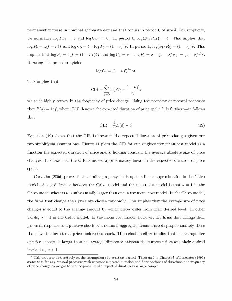
that E(d) = 1/f , where E(d) denotes the expected duration of price spells,31 it furthermore follows

that

CIR =δ

νE(d) − δ. (19)

Equation (19) shows that the CIR is linear in the expected duration of price changes given our

two simplifying assumptions. Figure 11 plots the CIR for our single-sector menu cost model as a

function the expected duration of price spells, holding constant the average absolute size of price

changes. It shows that the CIR is indeed approximately linear in the expected duration of price

spells.

Carvalho (2006) proves that a similar property holds up to a linear approximation in the Calvo

model. A key difference between the Calvo model and the menu cost model is that ν = 1 in the

Calvo model whereas ν is substantially larger than one in the menu cost model. In the Calvo model,

the firms that change their price are chosen randomly. This implies that the average size of price

changes is equal to the average amount by which prices differ from their desired level. In other

words, ν = 1 in the Calvo model. In the menu cost model, however, the firms that change their

prices in response to a positive shock to a nominal aggregate demand are disproportionately those

that have the lowest real prices before the shock. This selection effect implies that the average size

of price changes is larger than the average difference between the current prices and their desired

levels, i.e., ν > 1.31This property does not rely on the assumption of a constant hazard. Theorem 1 in Chapter 5 of Lancaster (1990)

states that for any renewal processes with constant expected duration and finite variance of durations, the frequencyof price change converges to the reciprocal of the expected duration in a large sample.

24

In general, menu cost models need not generate a convex relationship between the frequency

of price change and the degree of monetary non-neutrality. This relationship can be linear or

concave if the selection effect is strong enough. One way to increase the strength of the selection

effect is to raise the average inflation rate and lower the variance of the idiosyncratic shocks.

Intuitively, this moves the model closer to the assumptions in Caplin and Spulber (1987). Figure

12 plots the variance of value added output as a function of the frequency of price change for a

high inflation/small idiosyncratic shocks case—specifically, µ = 0.01 and σε = 0.01—as well as for

our benchmark calibration—µ = 0.002 and σε = 0.0425. In the high inflation/small idiosyncratic

shocks case, the degree of monetary non-neutrality is smaller than in the benchmark calibration for

each frequency of price change. Furthermore, the degree of monetary non-neutrality is much less

convex in the frequency of price change than it is in our benchmark calibration.

4.2 Heterogeneity and Sectoral Output

The relatively modest response of aggregate value-added output to aggregate demand shocks in the

model without intermediate inputs masks much larger responses of output in individual sectors.

Figure 13 plots the response of aggregate output and sectoral output to an expansionary demand

shock in our 14 sector model without intermediate inputs. The sectoral responses vary greatly.

Output in the sectors with most price rigidity rises by several times as much as aggregate output,

while output in the sectors with most price flexibility falls sharply.

In the model without intermediate inputs, the desired price of all firms rises approximately

one-for-one in percentage terms with nominal aggregate demand and is approximately independent

of the prices charged by other firms—equation (17) with sm = 0. As a consequence, the sectoral

price index in sectors with a high frequency of price change—such as gasoline—quickly rises pro-

portionally to the shock, while the sectoral price index in sectors with more rigid prices adjusts

more slowly. This causes the prices in the sectors with most flexible prices to rise sharply relative

to the prices in the sectors with more rigid prices. This change in relative prices leads consumers

to shift expenditures toward the sectors in which prices are more rigid. In the model without

intermediate inputs, this expenditure switching effect is strong enough that output in the sectors

with most flexible prices falls after the demand shock. We simulate the model for 600 periods and

find that the heterogeneity in price flexibility implies that the correlation of output in different

25

sectors with aggregate output ranges from -0.99 to 0.95, with output in the sticky price sectors

being highly positively correlated with aggregate output while output in the flexible price sectors

is highly negatively correlated with aggregate output.32

In contrast, in the model with intermediate goods, a firm’s desired price is heavily dependent

on the prices of other firms—equation (17) with sm = 0.75. Since the prices of other firms make up

a large component of the marginal costs of all firms, the higher are other firms’ prices, the higher is

any particular firm’s desired price. This leads to a strikingly different response of sectoral output

to aggregate demand shocks.

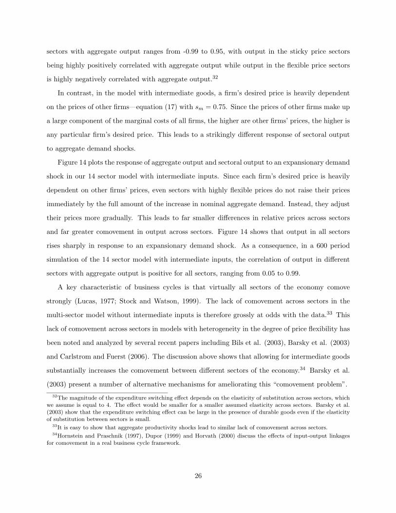
Figure 14 plots the response of aggregate output and sectoral output to an expansionary demand

shock in our 14 sector model with intermediate inputs. Since each firm’s desired price is heavily

dependent on other firms’ prices, even sectors with highly flexible prices do not raise their prices

immediately by the full amount of the increase in nominal aggregate demand. Instead, they adjust

their prices more gradually. This leads to far smaller differences in relative prices across sectors

and far greater comovement in output across sectors. Figure 14 shows that output in all sectors

rises sharply in response to an expansionary demand shock. As a consequence, in a 600 period

simulation of the 14 sector model with intermediate inputs, the correlation of output in different

sectors with aggregate output is positive for all sectors, ranging from 0.05 to 0.99.

A key characteristic of business cycles is that virtually all sectors of the economy comove

strongly (Lucas, 1977; Stock and Watson, 1999). The lack of comovement across sectors in the

multi-sector model without intermediate inputs is therefore grossly at odds with the data.33 This

lack of comovement across sectors in models with heterogeneity in the degree of price flexibility has

been noted and analyzed by several recent papers including Bils et al. (2003), Barsky et al. (2003)

and Carlstrom and Fuerst (2006). The discussion above shows that allowing for intermediate goods

substantially increases the comovement between different sectors of the economy.34 Barsky et al.

(2003) present a number of alternative mechanisms for ameliorating this “comovement problem”.32The magnitude of the expenditure switching effect depends on the elasticity of substitution across sectors, which

we assume is equal to 4. The effect would be smaller for a smaller assumed elasticity across sectors. Barsky et al.(2003) show that the expenditure switching effect can be large in the presence of durable goods even if the elasticityof substitution between sectors is small.

33It is easy to show that aggregate productivity shocks lead to similar lack of comovement across sectors.34Hornstein and Praschnik (1997), Dupor (1999) and Horvath (2000) discuss the effects of input-output linkages

for comovement in a real business cycle framework.

26

4.3 Product Introduction

The menu cost model we have been analyzing up until now in this paper implicitly assumes that

products are infinitely lived. In fact, however, product turnover is quite rapid in certain sectors of

the economy. When a firm introduces a new product, it must necessarily set a new price for this

product. Rapid product turnover can therefore affect the degree of price flexibility in the economy.

Furthermore, since firms can often anticipate future product turnover—e.g., fall-spring turnover

in apparel—they may decide not to incur the fixed cost needed to change the price of an existing

product.

Table 10 reports the frequency of product substitution for the sectors in our multi-sector models.

35 Table 10 reveals that product substitution is a frequent occurrence in several categories

of durable goods—Apparel, Transportation Goods (Cars), Household Furnishing and Recreation

Goods—but less frequent for other products. A number of these categories—especially Apparel—

have a very low frequency of price change. Since our results regarding amplification due to hetero-

geneity rely heavily outlying sectors such as Apparel, it is important to understand how accounting

for product flexibility affects our results.

Many factors influence a firm’s decision about the introduction of a new product. These include

seasonality, development cycles, innovation and random shifts in consumer tastes. Figure 15 plots

the frequency of product substitution across different months of the year for the four categories

for which product substitution is most frequent. In Apparel, seasonal variation in tastes seems to

be a dominant factor in the timing of product introduction. In the automobile industry, product

introduction seems to be heavily influenced by a yearly development cycle with new models being

introduced in the fall of each year.

This evidence suggests that product turnover may be largely orthogonal to a firm’s desire to

change its price and to macroeconomic conditions. A computationally tractable way of modelling

this type of event is to consider a model in which new products arrive according to an exogenous

Poisson process. This model is equivalent to the CalvoPlus model where Kl = 0 and 1− α in each35Ideally we would have a measure of the rate of product introduction since pricing decisions are made when new

products are introduced. However, the BLS does not tract the introduction of new products. When a product thatthe BLS has been tracking becomes permanently unavailable, the BLS agent is instructed to substitute to the mostsimilar existing product. In most cases this product will have existed for some time. If the hazard of product exitis upward sloping, the frequency of product substitution is therefore an upward biased measure of the frequency ofproduct introduction.

27

sector is equal to the frequency of product substitution. The menu cost in the high cost state is

calibrated so that the frequency of high cost price changes in the model matches the frequency of

price change in the data for each sector.

Table 13 shows that product turnover associated with factors unrelated to the firms’ pricing

decisions have little effect on the monetary non-neutrality implied by the model. This is because the

“selection effect” applies only to the regular price changes. While new fashions are priced to keep

up with inflation, they are not (in this model) introduced because the old fashions were mispriced.

For comparison purposes, table 13 also presents results for a calibration of the menu cost model

where we treat product introductions as if they were in the same as regular price changes. In

this case, the shorter durations of prices associated with “product flexibility” would have a much

larger effect on monetary non-neutrality. In either case, the inclusion of product substitutions in

the model has little effect on the amplification effect associated with heterogeneity.

5 Conclusion

This paper analyzes the responsiveness of real output to monetary shocks in a multi-sector menu

cost model that allows for intermediate goods. We calibrate the model to new evidence on the

frequency of non-sale price changes from Nakamura and Steinsson (2006). We find that hetero-

geneity across sectors approximately triples the monetary non-neutrality in the model relative to

a one-sector model calibrated to the mean frequency of price change across all goods. Intuitively,

the magnification arises because the degree of monetary non-neutrality in a one-sector model is a

convex function of the frequency of price change, implying that greater heterogeneity increases the

average degree of monetary non-neutrality. The degree of monetary non-neutrality in the multi-

sector model with intermediate goods is comparable to the degree of monetary non-neutrality of a

single-sector model calibrated to match the median frequency of price change.

Allowing for intermediate goods generates strategic complementarity in the menu cost model.

The menu cost model with intermediate inputs generates three times as much monetary non-

neutrality as a corresponding model without intermediate inputs. Incorporating strategic com-

plementarities into menu cost models designed to fit the size and frequency of micro-level price

changes has proven challenging. Standard sources of strategic complementarity—such as fixed fac-

tors of production and non-isoelastic demand curves—yield price changes that are much too small

28

on average for reasonable parameter values. This is not the case for intermediate inputs. Allowing

for intermediate goods generates strategic complementarities without requiring unrealistically large

variation in marginal costs or menu costs.

We also develop an extension of the Calvo model designed to fit the microeconomic evidence on

the size and frequency of price change, while still maintaining the idea that the timing of some price

changes is random rather than occurring in response to changes in costs. We refer to this model

as the CalvoPlus model. The effects of heterogeneity and intermediate goods on monetary non-

neutrality in the CalvoPlus model are similar to the effects in the benchmark menu cost model. We

show that the relatively large amount of monetary non-neutrality generated by the Calvo model is

quite sensitive to even a modest amount of selection by firms regarding the timing of price changes.

When 75% of price changes occur in the low menu cost state, the CalvoPlus model generates about

double the amount of monetary non-neutrality generated by the menu cost model—about 1/3 of

the monetary non-neutrality generated in the Calvo limit.

29

A Profit Function

Cost minimization by firm z implies that labor demand and demand for the composite intermediate

input be governed byWt

Pt= (1 − sm)AtLt(z)−smMt(z)smΩt(z),

1 = smAtLt(z)1−smMt(z)sm−1Ωt(z),

where Ωt(z) denotes the marginal costs of firm z at time t. Combining these two equations yields

Wt

Pt=

1 − smsm

Mt(z)Lt(z)

. (20)

Using this equation we can rewrite the profits of firm z in period t as

ΠRt (z) =

(pt(z)Pt

)yt(z) −

(Wt

Pt

)Lt(z) −Mt(z) −K

(Wt

Pt

)It(z)

=(pt(z)Pt

)yt(z) −

11 − sm

(Wt

Pt

)Lt(z) −K

(Wt

Pt

)It(z).

Combining the production function—equation (8)—and equation (20) yields

Lt(z) =(yt(z)At(z)

) (sm

1 − sm

)−sm(Wt

Pt

)−sm

.

Using this equation, we can rewrite profits as

ΠRt (z) =

(pt(z)Pt

)yt(z) − (1 − sm)sm−1s−sm

m

(Wt

Pt

)1−sm(yt(z)At(z)

)−K

(Wt

Pt

)It(z). (21)

Using the firm’s demand curve—equation (12)—and the labor supply curve—equation (7)—we can

rewrite profits as

ΠRt (z) = Yt

(pt(z)Pt

)1−θ− (1 − sm)sm−1s−sm

m ω1−smLψ(1−sm)t C

γ(1−sm)t

(1

At(z)

)Yt

(pt(z)Pt

)−θ−KωLψt C

γt It(z).

Finally, log-linear approximations of Yt = Ct+∫ 10 Mt(z)dz, the production function and labor supply

around the steady state with flexible prices yield Yt = a1Ct and Lt = a2Ct. Here Yt = log(Yt/Y )

and Y denotes the steady state of Yt with flexible prices. Ct and Lt are defined analogously. Using

these log-linear approximations and the fact that Ct = St/Pt, we can rewrite profits as a function

of (At(z), pt−1(z)/Pt, St/Pt) and pt(z).

30

B Stationary Distribution

We solve for the stationary distribution over the state space of the firm’s problem using the following

algorithm:

0. Start with an initial distribution Q(A(z), p−1(z)/P, S/P ). We use a uniform distribution as

our initial distribution.

1. Map Q(A(z), p−1(z)/P, S/P ) into Q(A(z), p(z)/P, S/P ) using the policy function F .

2. Map Q(A(z), p(z)/P, S/P ) into Q(A+1(z), p(z)/P, S/P ) using the transition probability ma-

trix for the technology process.

3. Map Q(A+1(z), p(z)/P, S/P ) into Q(A+1(z), p(z)/P, S+1/P ) using the probability transition

matrix for the nominal aggregate demand process.

4. Map Q(A+1(z), p(z)/P, S+1/P ) into Q(A+1(z), p(z)/P+1, S+1/P+1) using the function Γ.

5. Check whether |Q(A+1(z), p(z)/P+1, S+1/P+1) −Q(A(z), p−1(z)/P, S/P )| < ξ where | · | de-

notes a sup-norm. If so, stop. If not, go back to step one.

31

References

Akerlof, G. A., and J. L. Yellen (1985): “A Near Rational Model of the Business Cycle, WithPrice and Wage Inertia,” Quarterly Journal of Economics, 100, 823–838.

Alvarez, L. J., P. Burriel, and I. Hernando (2005a): “Do Decreasing Hazard Functions forPrice Changes Make Sense?,” Working Paper No. 461, European Central Bank.

Alvarez, L. J., E. Dhyne, M. M. Hoeberichts, C. Kwapil, H. L. Bihan, P. Lunnemann,

F. Martins, R. Sabbatini, H. Stahl, P. Vermeulen, and J. Vilmunen (2005b): “StickyPrices in the Euro Area: A summary of New Micro Evidence,” Working Paper No. 563, EuropeanCentral Bank.

Andrews, D. W., and H.-Y. Chen (1994): “Approximately Median-Unbiased Estimation ofAutoregressive Models,” Journal of Business and Economic Statistics, 12(2), 187–204.

Bakhshi, H., P. Burriel-Llombart, H. Khan, and B. Rudolf (2006): “The New KeynesianPhillips Curve under Trend Inflation and Strategic Complementarity,” Journal of Macroeco-nomics, Forthcoming.

Ball, L., and D. Romer (1990): “Real Rigidities and the Non-neutrality of Money,” Review ofEconomic Studies, 57(2), 183–204.

(1991): “Sticky Prices and a Coordination Failure,” American Economic Review, 81(3),539–552.

Barro, R. J. (1972): “A Theory of Monopolistic Price Adjustment,” Review of Economic Studies,39(1), 17–26.

Barsky, R., C. L. House, and M. Kimball (2003): “Do Flexible Durable Goods Prices Under-mine Sticky Price Models?,” NBER Working Paper No. 9832.

Basu, S. (1995): “Intermediate Goods and Business Cycles: Implications for Productivity andWelfare,” American Economic Review, 85(3), 512–531.

Baumgartner, J., E. Glatzer, F. Rumler, and A. Stiglbauer (2005): “How Frequently doConsumer Prices Change in Austria?,” Working Paper No. 523, European Central Bank.

Bergin, P. R., and R. C. Feenstra (2000): “Staggered Price Setting, Translog Preferences,and Endogenous Persistence,” Journal of Monetary Economics, 45, 657–680.

Berry, S., J. Levinsohn, and A. Pakes (1995): “Automobile Prices in Market Equilibrium,”Econometrica, 63(4), 841–890.

Bils, M., and P. J. Klenow (2002): “Some Evidence on the Importance of Sticky Prices,” NBERWorking Paper No. 9069.

(2004): “Some Evidence on the Importance of Sticky Prices,” Journal of Political Eco-nomics, 112(5), 947–985.

Bils, M., P. J. Klenow, and O. Kryvtsov (2003): “Sticky Prices and Monetary Policy Shocks,”Federal Reserve Mank of Minneapolis Quarterly Review, 27(1), 2–9.

32

Blanchard, O. J. (1983): “Price Asynchronization and Price-Level Inertia,” in Inflation, Debtand Indexation, ed. by R. Dornbusch, and M. H. Simonson. MIT Press, Cambridge, MA.

(1987): “Aggregate and Individual Price Adjustment,” Brookings Papers on EconomicActivity, (1), 57–109.

Blinder, A. S., E. R. D. Canetti, D. E. Lebow, and J. B. Rudd (1998): Asking AboutPrices. Russell Sage Foundation, New York, New York.

Broda, C., and D. E. Weinstein (2006): “Globalization and the Gains from Variety,” QuarterlyJournal of Economics, 121(4), 541–585.

Burstein, A. T. (2005): “Inflation and output dynamics with state-dependent pricing decisions,”Journal of Monetary Economics, Forthcoming.

Burstein, A. T., and C. Hellwig (2006): “Prices and Market Share in a Menu Cost Model,”Working Paper, UCLA.

Caballero, R. J., and E. M. Engel (1991): “Dynamic (S,s) Economies,” Econometrica, 59(6),1659–1686.

(1993): “Heterogeneity and Output Fluctuations in a Dynamic Menu-Cost Economy,”Review of Economic Studies, 60, 95–119.

(2006): “Price Stickiness in Ss Models: Basic Properties,” Working Paper, MIT.

Calvo, G. A. (1983): “Staggered Prices in a Utility-Maximizing Framework,” Journal of MonetaryEconomics, 12, 383–398.

Caplin, A., and J. Leahy (1991): “State-Dependent Pricing and the Dynamics of Money andOutput,” Quarterly Journal of Economics, 106(3), 683–708.

(1997): “Aggregation and Optimization with State-Dependent Pricing,” Econometrica,65(3), 601–625.

Caplin, A., and D. Spulber (1987): “Menu Costs and the Neutrality of Money,” QuarterlyJournal of Economics, 102(4), 703–725.

Carlstrom, C. T., and T. S. Fuerst (2006): “Co-Movement in Sticky Price Models withDurable Goods,” Working Paper.

Carlton, D. W. (1986): “The Rigidity of Prices,” American Economic Review, 76(4), 637–658.

Carvalho, C. (2006): “Heterogeneity in Price Stickiness and the New Keynesian Phillips Curve,”Working Paper, Princeton University.

Chari, V., P. J. Kehoe, and E. R. McGrattan (1996): “Sticky Price Models of the BusinessCycle: Can the Contract Multiplier Solve the Persistence Problem,” NBER Working Paper No.5809.

(2000): “Sticky Price Models of the Business Cycle: Can the Contract Multiplier Solvethe Persistence Problem,” Econometrica, 68(5), 1151–1179.

33

Christiano, L., M. Eichenbaum, and C. Evans (2005): “Nominal Rigidities and the DynamicEffects of a Shock to Monetary Policy,” Journal of Political Economics, 115, 1–45.

Clarida, R., J. Gali, and M. Gertler (1999): “The Science of Monetary Policy: A NewKeynesian Perspective,” Journal of Economic Literature, 37, 1661–1707.

Danziger, L. (1999): “A Dynamic Economy with Costly Price Adjustments,” American EconomicReview, 89, 878–901.

Dhyne, E., L. J. Alvarez, H. L. Bihan, G. Veronese, D. Dias, J. Hoffmann, N. Jonker,

P. Lunnemann, F. Rumler, and J. Vilmunen (2006): “Price Setting in the Euro Area andthe United States: Some Facts From Individual Consumer Price Data,” Journal of EconomicPerspectives, 20(2), 171–192.

Dias, D. A., C. Robalo Marques, and J. M. Santo Silva (2005): “Time or State DependentPrice Setting Rules? Evidence from Portuguese Micro Data,” Working Paper No. 511, EuropeanCentral Bank.

Dixit, A. K., and R. S. Pindyck (1994): Investment Under Uncertainty. Princeton UniversityPress, Princeton, NJ.

Dotsey, M., R. King, and A. Wolman (1999): “State-Dependent Pricing and the GeneralEquilibrium Dynamics of Money and Output,” Quarterly Journal of Economics, 114(2), 655–690.

Dupor, B. (1999): “Aggregation and Irrelevance in Multi-Sector Models,” Journal of MonetaryEconomics, 43, 391–409.

Fougere, D., H. L. Bihan, and P. Sevestre (2005): “Heterogeneity in Consumer Price Stick-iness: A Microeconometric Investigation,” Working Paper No. 536, European Central Bank.

Gertler, M., and J. Leahy (2006): “A Phillips Curve with an Ss Foundation,” Working Paper,New York University.

Golosov, M., and R. E. Lucas (2006): “Menu Costs and Phillips Curves,” Working Paper,MIT.

Hansen, G. D. (1985): “Indivisible Labor and the Business Cycle,” Journal of Monetary Eco-nomics, 16, 309–327.

Hornstein, A., and J. Praschnik (1997): “Intermediate Inputs and Sectoral Comovement inthe Business Cycle,” Journal of Monetary Economics, 40, 573–595.

Horvath, M. (2000): “Sectoral Shocks and Aggregate Fluctuations,” Journal of Monetary Eco-nomics, 45, 69–106.

John, A. A., and A. L. Wolman (2004): “An Inquiry into the Existence and Uniqueness ofEquilibrium with State-Dependent Pricing,” Federal Reserve Bank of Richmond Working PaperNo. 04-04.

Jonker, N., C. Folkertsma, and H. Blijenberg (2004): “An Empirical Analysis of PriceSetting Behavior in the Netherlands in the Period 1998-2003 Using Micro Data,” Working PaperNo. 413, European Central Bank.

34

Kimball, M. (1995): “The Quantitative Analytics of the Basic Neomonetarist Model,” Journalof Money, Credit and Banking, 27(4), 1241–1277.

Klenow, P. J., and O. Kryvtsov (2005): “State-Dependent or Time-Dependent Pricing: DoesIt Matter for Recent U.S. Inflation,” Working Paper, Stanford University.

Klenow, P. J., and J. L. Willis (2006): “Real Rigidities and Nominal Price Changes,” WorkingPaper, Stanford University.

Krusell, P., and A. Smith (1998): “Income and Wealth Heterogeneity in the Macroeconomy,”Journal of Political Economics, 106(5), 867–896.

Lancaster, T. (1990): The Econometric Analysis of Transition Data. Cambridge UniversityPress, Cambridge, U.K.

Lucas, R. E. (1977): “Understanding Business Cycles,” Carnegie-Rochester Series on PublicPolicy, 5, 7–29.

Mankiw, G. N. (1985): “Small Menu Costs and Large Business Cycles: A Macroeconomic Modelof Monopoly,” Quarterly Journal of Economics, 100, 529–539.

Midrigan, V. (2005): “Menu Costs, Multi-Product Firms, and Aggregate Fluctuations,” WorkingPaper, Ohio State University.

Nakamura, E., and J. Steinsson (2006): “Five Facts about Prices: A Reevaluation of MenuCost Models,” Working Paper, Harvard University.

Nevo, A. (2001): “Measuring Market Power in the Ready-to-Eat Cereal Industry,” Econometrica,69(2), 307–342.

Rogerson, R. (1988): “Indivisble Labor, Lotteries and Equilibrium,” Journal of Monetary Eco-nomics, 21, 3–16.

Rotemberg, J. J., and M. Woodford (1995): “Dynamic General Equilibrium Models withImperfectly Competitive Product Markets,” in Frontiers of Business Cycle Research, ed. byT. F. Cooley, pp. 243–293, Princeton, NJ. Princeton University Press.

(1997): “An Optimization-Based Econometric Framework for the Evaluation of MonetaryPolicy,” in NBER Macroeconomics Annual 1997, ed. by B. S. Bernanke, and J. J. Rotemberg,pp. 297–346, Cambridge, MA. MIT Press.

Ryan, S. P. (2006): “The Costs of Environmental Regulation in a Concentrated Industry,” Work-ing Paper, MIT.

Sheshinski, E., and Y. Weiss (1977): “Inflation and Costs of Price Adjustment,” Review ofEconomic Studies, 44(2), 287–303.

Smets, F., and R. Wouters (2003): “An Estimated Dynamic Stochastic General EquilibriumModel of the Euro Area,” Journal of the European Economic Association, 1(5), 1123–1175.

Stock, J. H., and M. W. Watson (1999): “Business Cycle Fluctuations in U.S. MacroeconomicTime Series,” in Handbook of Macroeconomics, ed. by J. B. Taylor, and M. Woodford, pp. 3–64,Amsterdam, The Netherlands. Elsevier.

35

Tauchen, G. (1986): “Finite State Markov-Chain Approximation to Univariate and Vector Au-toregressions,” Economics Letters, 20(2), 177–181.

Taylor, J. B. (1980): “Aggregate Dynamics and Staggered Contracts,” Journal of Political Eco-nomics, 88, 1–23.

Willis, J. L. (2003): “General Equilibrium of a Monetary Model with State-Dependent Pricing,”Working Paper.

Woodford, M. (2003): Interest and Prices. Princeton University Press, Princeton, NJ.

Zbaracki, M. J., M. Ritson, D. Levy, S. Dutta, and M. Bergin (2004): “Managerial andCustomer Costs of Price Adjuestment: Direct Evidence from Industry Markets,” 86(2), 514–533.

36

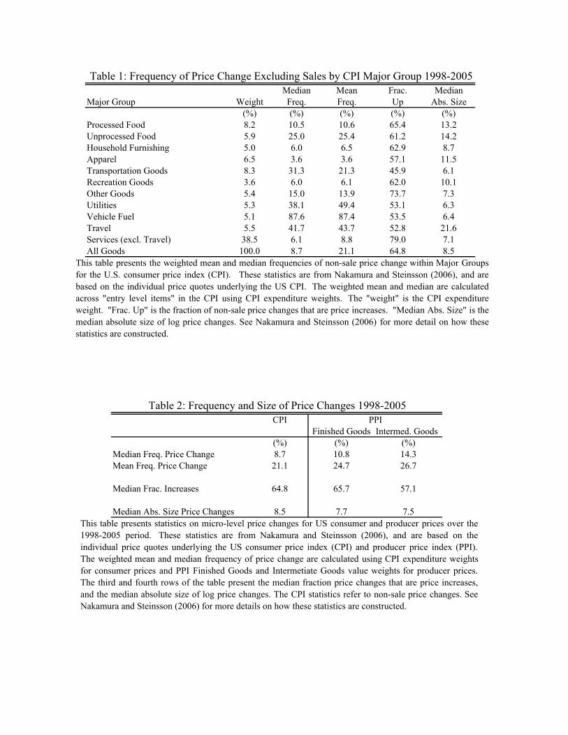
Median Mean Frac. MedianMajor Group Weight Freq. Freq. Up Abs. Size

(%) (%) (%) (%) (%)Processed Food 8.2 10.5 10.6 65.4 13.2Unprocessed Food 5.9 25.0 25.4 61.2 14.2Household Furnishing 5.0 6.0 6.5 62.9 8.7Apparel 6.5 3.6 3.6 57.1 11.5Transportation Goods 8.3 31.3 21.3 45.9 6.1Recreation Goods 3.6 6.0 6.1 62.0 10.1Other Goods 5.4 15.0 13.9 73.7 7.3Utilities 5.3 38.1 49.4 53.1 6.3Vehicle Fuel 5.1 87.6 87.4 53.5 6.4Travel 5.5 41.7 43.7 52.8 21.6Services (excl. Travel) 38.5 6.1 8.8 79.0 7.1All Goods 100.0 8.7 21.1 64.8 8.5

Table 1: Frequency of Price Change Excluding Sales by CPI Major Group 1998-2005

This table presents the weighted mean and median frequencies of non-sale price change within Major Groupsfor the U.S. consumer price index (CPI). These statistics are from Nakamura and Steinsson (2006), and arebased on the individual price quotes underlying the US CPI. The weighted mean and median are calculatedacross "entry level items" in the CPI using CPI expenditure weights. The "weight" is the CPI expenditureweight. "Frac. Up" is the fraction of non-sale price changes that are price increases. "Median Abs. Size" is themedian absolute size of log price changes. See Nakamura and Steinsson (2006) for more detail on how thesestatistics are constructed.

CPIFinished Goods Intermed. Goods

(%) (%) (%)Median Freq. Price Change 8.7 10.8 14.3Mean Freq. Price Change 21.1 24.7 26.7

Median Frac. Increases 64.8 65.7 57.1

Median Abs. Size Price Changes 8.5 7.7 7.5This table presents statistics on micro-level price changes for US consumer and producer prices over the1998-2005 period. These statistics are from Nakamura and Steinsson (2006), and are based on theindividual price quotes underlying the US consumer price index (CPI) and producer price index (PPI).The weighted mean and median frequency of price change are calculated using CPI expenditure weightsfor consumer prices and PPI Finished Goods and Intermetiate Goods value weights for producer prices.The third and fourth rows of the table present the median fraction price changes that are price increases,and the median absolute size of log price changes. The CPI statistics refer to non-sale price changes. SeeNakamura and Steinsson (2006) for more details on how these statistics are constructed.

PPITable 2: Frequency and Size of Price Changes 1998-2005

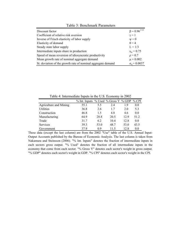
Discount factor β = 0.961/12

Coefficient of relative risk aversion γ = 1Inverse of Frisch elasticity of labor supply ψ = 0Elasticity of demand θ = 4Steady state labor supply L = 1/3Intermediate inputs share in production sm = 0.75Speed of mean reversion of idiosyncratic productivity ρ = 0.7Mean growth rate of nominal aggregate demand μ = 0.002St. deviation of the growth rate of nominal aggregate demand ση = 0.0037

Table 3: Benchmark Parameters

% Int. Inputs % Used % Gross Y % GDP % CPIAgriculture and Mining 55.1 5.5 2.4 1.9 0.0Utilities 36.8 2.6 1.7 2.0 5.3Construction 46.8 1.5 4.8 4.6 0.0Manufacturing 64.9 28.8 20.5 12.9 51.2Trade 31.7 6.2 10.4 12.8 0.0Services 39.3 53.0 48.7 53.0 43.5Government 37.9 0.9 11.5 12.8 0.0

Table 4: Intermediate Inputs in the U.S. Economy in 2002

These data (except the last column) are from the 2002 "Use" table of the U.S. Annual Input-Output Accounts published by the Bureau of Economic Analysis. The last column is taken fromNakamura and Steinsson (2006). "% Int. Inputs" denotes the fraction of intermediate inputs ineach sectors gross output. "% Used" denotes the fraction of all intermediate inputs in theeconomy that come from each sector. "% Gross Y" denotes each sector's weight in gross output."% GDP" denotes each sector's weight in GDP. "% CPI" denotes each sector's weight in the CPI.

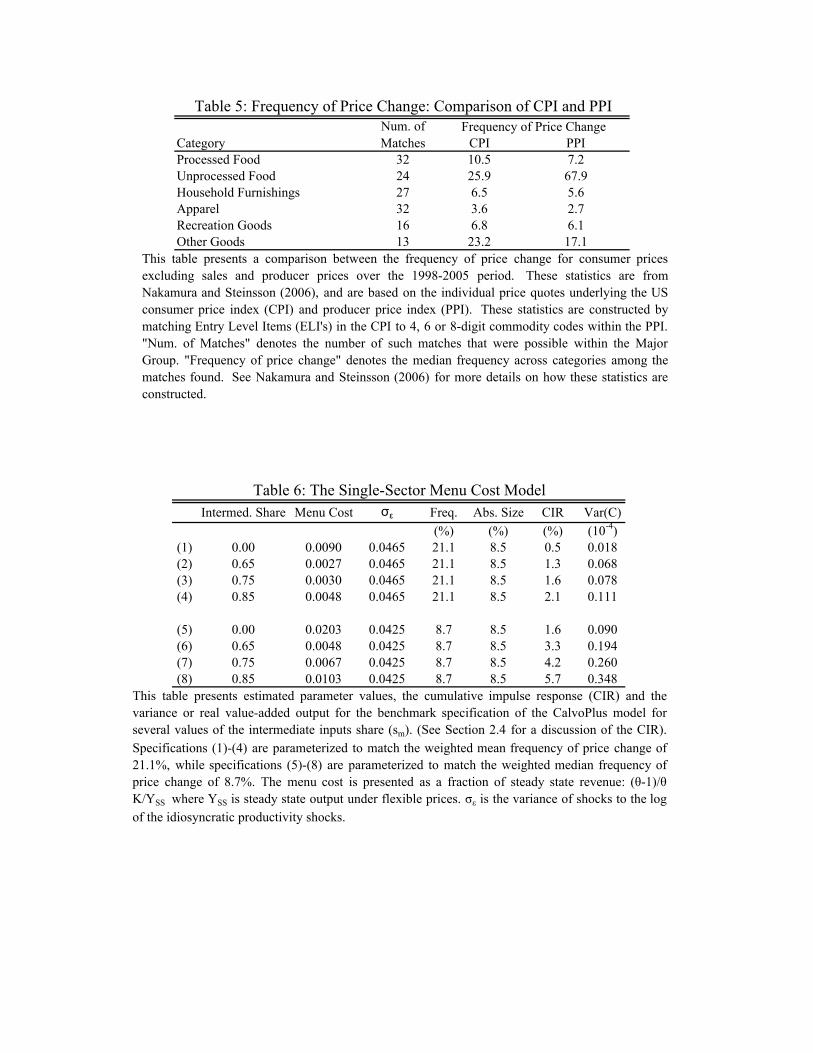
Category CPI PPIProcessed Food 32 10.5 7.2Unprocessed Food 24 25.9 67.9Household Furnishings 27 6.5 5.6Apparel 32 3.6 2.7Recreation Goods 16 6.8 6.1Other Goods 13 23.2 17.1

This table presents a comparison between the frequency of price change for consumer pricesexcluding sales and producer prices over the 1998-2005 period. These statistics are fromNakamura and Steinsson (2006), and are based on the individual price quotes underlying the USconsumer price index (CPI) and producer price index (PPI). These statistics are constructed bymatching Entry Level Items (ELI's) in the CPI to 4, 6 or 8-digit commodity codes within the PPI."Num. of Matches" denotes the number of such matches that were possible within the MajorGroup. "Frequency of price change" denotes the median frequency across categories among thematches found. See Nakamura and Steinsson (2006) for more details on how these statistics areconstructed.

Table 5: Frequency of Price Change: Comparison of CPI and PPINum. of Matches

Frequency of Price Change

Intermed. Share Menu Cost σε Freq. Abs. Size CIR Var(C)(%) (%) (%) (10-4)

(1) 0.00 0.0090 0.0465 21.1 8.5 0.5 0.018(2) 0.65 0.0027 0.0465 21.1 8.5 1.3 0.068(3) 0.75 0.0030 0.0465 21.1 8.5 1.6 0.078(4) 0.85 0.0048 0.0465 21.1 8.5 2.1 0.111

(5) 0.00 0.0203 0.0425 8.7 8.5 1.6 0.090(6) 0.65 0.0048 0.0425 8.7 8.5 3.3 0.194(7) 0.75 0.0067 0.0425 8.7 8.5 4.2 0.260(8) 0.85 0.0103 0.0425 8.7 8.5 5.7 0.348

Table 6: The Single-Sector Menu Cost Model

This table presents estimated parameter values, the cumulative impulse response (CIR) and thevariance or real value-added output for the benchmark specification of the CalvoPlus model forseveral values of the intermediate inputs share (sm). (See Section 2.4 for a discussion of the CIR).Specifications (1)-(4) are parameterized to match the weighted mean frequency of price change of21.1%, while specifications (5)-(8) are parameterized to match the weighted median frequency ofprice change of 8.7%. The menu cost is presented as a fraction of steady state revenue: (θ-1)/θK/YSS where YSS is steady state output under flexible prices. σε is the variance of shocks to the logof the idiosyncratic productivity shocks.

θ α Menu Cost σε Freq. Frac. Abs. Size CIR(%) (%) (%) (%)

(1) 7 1 0.0386 0.0415 8.7 66.6 8.5 1.5(2) 7 2/3 0.0257 0.0415 8.7 85.4 3.2 3.5(3) 7 2/3 0.1774 0.1250 8.7 67.4 8.5 3.4

Table 7: The Single-Sector Menu Cost Model With Diminishing Returns to Scale

This table presents the parameter values and cumulative impulse reponse (CIR) for the menu cost modelboth with and without diminishing returns to labor. (See Section 2.4 for a discussion of the CIR). Allthe specifications are parameterized to match the weighted median frequency of price change 8.7%.The parameter α is the coefficient on labor in the production function. Specification (1) presents themodel without diminishing returns to labor where α=1. Specifications (2) and (3) present model withdiminishing returns to labor where α=2/3. Specification (2) maintains the same variance of theidiosyncratic shock as specification (1), while specification (3) adjusts the variance of the idiosyncraticshock to match the weighted median size of price changes, 8.5%. The menu cost is presented as afraction of steady state revenue: (θ-1)/θ K/YSS where YSS is steady state output under flexible prices. σε is the variance of shocks to the log of the firms' idiosyncratic productivity levels.

Frac. Abs.High Low σε Low Cost Freq. Size CIR Var(C)

(%) (%) (%) (%) (10-4)(1) 0.30 0 0.0425 99 8.7 2.8 9.9 0.659(2) 1.50 0 0.1700 99 8.7 7.2 10.2 0.699

(3) 0.340 0.0010 0.1100 89 8.7 8.5 5.1 0.312(4) 0.113 0.0025 0.0725 74 8.7 8.5 3.4 0.210(5) 0.049 0.0050 0.0545 54 8.7 8.5 2.4 0.135

Menu Cost

Table 8: Matching the Facts With the CalvoPlus Model

This table presents estimated parameter values, the cumulative impulse response (CIR) and the variance orreal value-added output (Var(C)) for the benchmark specification of the CalvoPlus model for several valuesof the intermediate inputs share (sm). (See Section 2.4 for a discussion of the CIR). The first two columnspresent the menu cost in the "high" and "low" menu cost states respectively. The fraction of time spent inthe "low menu cost" state is set at 1-α = 0.087 in all cases. The third column gives the variance of shocksto the log of the idiosyncratic productivity shocks σε. The fourth column gives the fraction of price changesthat occur in the low menu cost state. The fifth and six columns give the frequency and average absolutesize of log price changes implied by the model. In all cases, the parameters are set to match the weightedmedian frequency of price change 8.7%. The share of intermediate inputs in the production function is setto sm = 0 in all cases. The first two specifications imply that all price changes occur in the low menu coststate, while specifications (3)-(5) imply that some price changes occur in both the high and low menu cost st

Frac.High Low σε Low Cost Freq. Abs. Size CIR Var(C)

(%) (%) (%) (%) (10-4)(1) 0 0.0525 0.0013 0.0665 77 21.1 8.5 1.2 0.058(2) 0.65 0.0128 0.0003 0.0665 77 21.1 8.5 2.5 0.144(3) 0.75 0.1730 0.0043 0.0665 77 21.1 8.5 3.1 0.185(4) 0.85 0.0278 0.0007 0.0665 77 21.1 8.5 4.3 0.260

(5) 0 0.1095 0.0027 0.0725 73 8.7 8.5 3.3 0.195(6) 0.65 0.0255 0.0006 0.0725 73 8.7 8.5 6.4 0.409(7) 0.75 0.0356 0.0009 0.0725 73 8.7 8.5 7.9 0.496(8) 0.85 0.0563 0.0014 0.0725 73 8.7 8.5 11.4 0.834

This table presents estimated parameter values, the cumulative impulse response (CIR) and the variance orreal value-added output for the benchmark specification of the CalvoPlus model for several values of theintermediate inputs share (sm). (See Section 2.4 for a discussion of the CIR). The first two columns presentthe menu cost in the "high" and "low" menu cost states respectively. The "low" menu cost KL is set at 1/40 ofthe high menu cost KH in all cases. Specifications (1)-(4) are parameterized to match the weighted meanfrequency of price change of 21.1%, while specifications (5)-(8) are parameterized to match the weightedmedian frequency of price change of 8.7%. The fraction of time spent in the "low menu cost" state is set at 1-α = freq. in all cases. The third column gives the variance of shocks to the log of the idiosyncraticproductivity shocks σε. The fifth column gives the fraction of price changes that occur in the low menu coststate. The sixth and seventh columns give the frequency of price changes and the average absolute size ofprice changes implied by the model.

Intermediate Inputs Share

Menu Cost

Table 9: The CalvoPlus Model With and Without Intermediate Goods

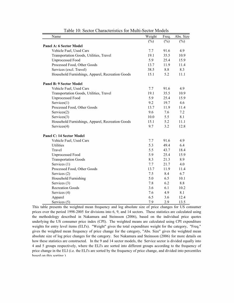
Name Weight Freq. Abs. Size(%) (%) (%)

Panel A: 6 Sector ModelVehicle Fuel, Used Cars 7.7 91.6 4.9Transportation Goods, Utilities, Travel 19.1 35.5 10.9Unprocessed Food 5.9 25.4 15.9Processed Food, Other Goods 13.7 11.9 11.4Services (excl. Travel) 38.5 8.8 8.3Household Furnishings, Apparel, Recreation Goods 15.1 5.2 11.1

Panel B: 9 Sector ModelVehicle Fuel, Used Cars 7.7 91.6 4.9Transportation Goods, Utilities, Travel 19.1 35.5 10.9Unprocessed Food 5.9 25.4 15.9Services(1) 9.2 19.7 4.6Processed Food, Other Goods 13.7 11.9 11.4Services(2) 9.6 7.6 7.2Services(3) 10.0 5.5 8.1Household Furnishings, Apparel, Recreation Goods 15.1 5.2 11.1Services(4) 9.7 3.2 12.8

Panel C: 14 Sector ModelVehicle Fuel, Used Cars 7.7 91.6 4.9Utilities 5.3 49.4 6.4Travel 5.5 43.7 18.4Unprocessed Food 5.9 25.4 15.9Transportation Goods 8.3 21.3 8.9Services (1) 7.7 21.7 4.0Processed Food, Other Goods 13.7 11.9 11.4Services (2) 7.5 8.4 6.7Household Furnishing 5.0 6.5 10.1Services (3) 7.8 6.2 8.8Recreation Goods 3.6 6.1 10.2Services (4) 7.6 4.9 8.1Apparel 6.5 3.6 12.4Services (5) 7.9 2.9 13.5

Table 10: Sector Characteristics for Multi-Sector Models

This table presents the weighted mean frequency and log absolute size of price changes for US consumerprices over the period 1998-2005 for divisions into 6, 9, and 14 sectors. These statistics are calculated usingthe methodology described in Nakamura and Steinsson (2006), based on the individual price quotesunderlying the US consumer price index (CPI). The weighted means are calculated using CPI expenditureweights for entry level items (ELI's). "Weight" gives the total expenditure weight for the category, "Freq."gives the weighted mean frequency of price change for the category, "Abs. Size" gives the weighted meanabsolute size of log price changes for the category. See Nakamura and Steinsson (2006) for more details onhow these statistics are constructed. In the 9 and 14 sector models, the Service sector is divided equally into4 and 5 groups respectively, where the ELI's are sorted into different groups according to the frequency ofprice change in the ELI (i.e. the ELI's are sorted by the frequency of price change, and divided into percentilesbased on this sorting )

K σε K σε Kh σε Kh σεx10-2 x10-2 x10-2 x10-2 x10-2 x10-2 x10-2 x10-2

Panel A: 6 Sector ModelVehicle Fuel, Used Cars 0.003 5.10 0.006 5.00 0.03 5.00 0.12 5.99Transp. Goods, Utilities, Travel 0.40 6.80 1.16 6.90 2.19 8.39 7.00 8.63Unprocessed Food 1.18 9.00 3.45 9.10 6.38 12.41 21.40 12.40Processed Food, Other Goods 1.22 5.80 3.60 5.70 5.73 8.69 20.40 9.20Services (excl. Travel) 0.85 4.10 2.30 3.90 4.98 7.10 12.75 6.75Hh. Furn., Apparel, Rec. Goods 1.32 4.00 6.47 5.46 9.01 9.00 35.70 9.85

Panel B: 9 Sector ModelVehicle Fuel, Used Cars 0.003 5.94 0.005 5.30 0.04 5.00 0.13 5.20Transp. Goods, Utilities, Travel 0.35 6.45 1.15 6.90 2.33 8.70 6.91 8.63Unprocessed Food 1.14 8.88 3.30 9.00 6.11 11.60 21.79 12.30Services(1) 0.16 2.80 0.37 2.40 0.69 3.40 2.45 3.76Processed Food, Other Goods 1.36 6.02 3.60 5.80 6.05 8.80 20.96 9.41Services(2) 0.57 3.15 3.50 4.00 4.73 6.50 13.00 6.10Services(3) 1.32 4.09 3.15 3.58 6.62 7.20 15.20 6.75Hh. Furn., Apparel, Rec. Goods 1.94 5.09 6.35 5.55 10.21 9.50 34.00 9.77Services(4) 3.91 6.39 11.50 6.19 17.01 11.60 53.00 11.31

Panel C: 14 Sector ModelVehicle Fuel, Used Cars 0.003 5.20 0.007 5.20 0.04 5.30 0.13 5.39Utilities 0.10 4.80 0.28 4.65 0.52 5.30 1.55 5.28Travel 0.78 12.00 1.95 11.10 5.04 14.00 14.00 14.00Unprocessed Food 1.18 9.00 3.70 9.40 6.93 12.20 21.20 12.40Transportation Goods 0.42 4.71 1.50 5.20 2.46 6.80 7.47 6.80Services (1) 0.16 2.97 0.41 2.70 0.54 3.20 1.45 3.00Processed Food, Other Goods 1.22 5.75 3.40 5.60 6.24 8.90 19.50 9.00Services (2) 0.59 3.30 1.70 3.20 3.15 5.69 10.00 5.70Household Furnishing 1.39 4.69 4.30 4.80 8.32 8.70 25.00 8.80Services (3) 1.10 4.10 3.30 4.10 6.43 7.60 18.50 7.40Recreation Goods 1.54 4.80 4.50 4.80 8.95 8.90 26.00 8.80Services (4) 1.26 4.00 3.40 3.80 7.31 7.20 22.50 7.60Apparel 3.23 5.99 9.52 6.05 15.44 10.54 40.00 10.50Services (5) 4.96 6.82 15.58 7.01 21.11 12.00 60.00 11.50

Menu Cost Model CalvoPlus ModelTable 11 : Parameter Values for Multi-Sector Models

This table presents the parameter values for the multi-sector menu cost model both with and without intermediate goods.The menu cost K is presented as a fraction of steady state revenue: (θ-1)/θ K/YSS where YSS is steady state output underflexible prices. σε is the variance of shocks to the log of the idiosyncratic productivity shocks. The first panel presents theparameters for the menu cost model both with and without intermediate goods; while the second panel presents theparameters for the CalvoPlus model with and without intermediate goods. sm is the fraction of marginal costs accounted forby intermediate goods. In the CalvoPlus model, the fraction of time spent in the "low menu cost" state is set at 1-α = freq.for each sector in all cases.

sm = 0.75 sm = 0 sm = 0.75 sm = 0

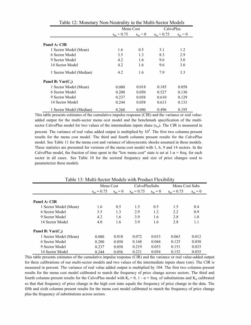
sm = 0.75 sm = 0 sm = 0.75 sm = 0

Panel A: CIR1 Sector Model (Mean) 1.6 0.5 3.1 1.26 Sector Model 3.5 1.3 8.3 2.99 Sector Model 4.2 1.6 9.6 3.014 Sector Model 4.2 1.6 9.6 3.0

1 Sector Model (Median) 4.2 1.6 7.9 3.3

Panel B: Var(Ct)1 Sector Model (Mean) 0.080 0.018 0.185 0.0586 Sector Model 0.200 0.050 0.527 0.1309 Sector Model 0.237 0.058 0.610 0.12914 Sector Model 0.244 0.058 0.613 0.133

1 Sector Model (Median) 0.260 0.090 0.496 0.195

Table 12: Monetary Non-Neutrality in the Multi-Sector ModelsMenu Cost CalvoPlus

This table presents estimates of the cumulative impulse response (CIR) and the variance or real value-added output for the multi-sector menu ocst model and the benchmark specification of the multi-sector CalvoPlus model for two values of the intermediate inputs share (sm). The CIR is measured inpercent. The variance of real value added output is multiplied by 104. The first two columns presentresults for the menu cost model. The third and fourth columns present results for the CalvoPlusmodel. See Table 11 for the menu cost and variance of idiosyncratic shocks assumed in these models.These statistics are presented for versions of the menu cost model with 1, 6, 9 and 14 sectors. In theCalvoPlus model, the fraction of time spent in the "low menu cost" state is set at 1-α = freq. for eachsector in all cases. See Table 10 for the sectoral frequency and size of price changes used toparameterize these models.

sm = 0.75 sm = 0 sm = 0.75 sm = 0 sm = 0.75 sm = 0

Panel A: CIR1 Sector Model (Mean) 1.6 0.5 1.5 0.5 1.5 0.46 Sector Model 3.5 1.3 2.9 1.2 2.2 0.99 Sector Model 4.2 1.6 3.9 1.6 2.8 1.014 Sector Model 4.0 1.6 3.9 1.6 2.8 1.1

Panel B: Var(Ct)1 Sector Model (Mean) 0.080 0.018 0.072 0.015 0.063 0.0126 Sector Model 0.200 0.050 0.168 0.044 0.125 0.0309 Sector Model 0.237 0.058 0.219 0.053 0.151 0.03314 Sector Model 0.244 0.056 0.221 0.054 0.152 0.035

This table presents estimates of the cumulative impulse response (CIR) and the variance or real value-added outputfor three calibrations of our multi-sector models and two values of the intermediate inputs share (sm). The CIR ismeasured in percent. The variance of real value added output is multiplied by 104. The first two columns presentresults for the menu cost model calibrated to match the frequency of price change across sectors. The third andfourth columns present results for the CalvoPlus model with Kl = 0, 1 - α = freq. of substitutions and Kh calibratedso that that frequency of price change in the high cost state equals the frequency of price change in the data. Thefifth and sixth columns present results for the menu cost model calibrated to match the frequency of price changeplus the frequency of substitutions across sectors.

Menu Cost SubsTable 13: Multi-Sector Models with Product Flexibility

Menu Cost CalvoPlusSubs

Figure 1: The Distribution of the Frequency of Price Change for U.S. Consumer Prices

This figure presents a histogram of the cross-sectional distribution of the frequency of non-sale price changes in U.S. consumer prices for the period 1998-2005 (percent per month). The figure is based on the statistics in Nakamura and Steinsson (2006). It is based on the individual price quotes underlying the US CPI. The figure shows the expenditure weighted distribution of the frequency of price changes across entry level items (ELI's) in the CPI.

0 10 20 30 40 50 60 70 80 90 1000

5

10

15

20

25

Frequency (probability per month)

% weight

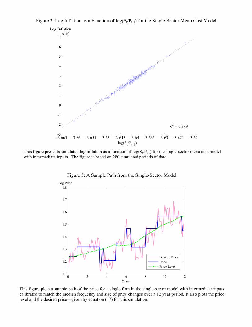
Figure 2: Log Inflation as a Function of log(St/Pt-1) for the Single-Sector Menu Cost Model This figure presents simulated log inflation as a function of log(St/Pt-1) for the single-sector menu cost model with intermediate inputs. The figure is based on 280 simulated periods of data.

-3.665 -3.66 -3.655 -3.65 -3.645 -3.64 -3.635 -3.63 -3.625 -3.62-3

-2

-1

0

1

2

3

4

5

6

7x 10

-3

log(St/Pt-1)

Log Inflation

R2 = 0.989

Figure 3: A Sample Path from the Single-Sector Model This figure plots a sample path of the price for a single firm in the single-sector model with intermediate inputs calibrated to match the median frequency and size of price changes over a 12 year period. It also plots the price level and the desired price—given by equation (17) for this simulation.

0 2 4 6 8 10 121.1

1.2

1.3

1.4

1.5

1.6

1.7

1.8

Years

Log Price

Desired PricePricePrice Level

Figure 4: Price Level Response to a Permanent Shock to Nominal Aggregate Demand

This figure presents the impulse response of the price level in response to a 1% shock to nominal aggregate demand for the single-sector model with intermediate inputs calibrated to the weighted median frequency of non-sale price changes.

-5 0 5 10 15 200

0.01

0.02

0.03

0.04

0.05

0.06

Months

Log Nom. Value-Added OutputLog Price Level

Figure 5: Output Response to a Permanent Shock to Nominal Aggregate Demand

This figure presents the response of real value-added output in response to a 1% shock to nominal aggregate demand for the single-sector model with intermediate inputs calibrated to the weighted median frequency of non-sale price changes.

-4 0 4 8 12 16 20 24-2

0

2

4

6

8

10x 10

-3

Months

Log Output

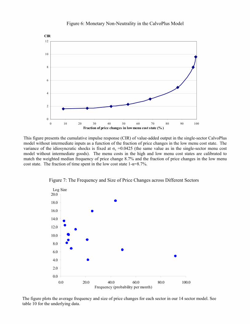
Figure 6: Monetary Non-Neutrality in the CalvoPlus Model

This figure presents the cumulative impulse response (CIR) of value-added output in the single-sector CalvoPlus model without intermediate inputs as a function of the fraction of price changes in the low menu cost state. The variance of the idiosyncratic shocks is fixed at σε =0.0425 (the same value as in the single-sector menu cost model without intermediate goods). The menu costs in the high and low menu cost states are calibrated to match the weighted median frequency of price change 8.7% and the fraction of price changes in the low menu cost state. The fraction of time spent in the low cost state 1-α=8.7%.

0

2

4

6

8

10

12

0 10 20 30 40 50 60 70 80 90 100Fraction of price changes in low menu cost state (% )

CIR

Figure 7: The Frequency and Size of Price Changes across Different Sectors The figure plots the average frequency and size of price changes for each sector in our 14 sector model. See table 10 for the underlying data.

0.0

2.0

4.0

6.0

8.0

10.0

12.0

14.0

16.0

18.0

20.0

0.0 20.0 40.0 60.0 80.0 100.0Frequency (probability per month)

Log Size

-4.65 -4.645 -4.64 -4.635 -4.63 -4.625 -4.62 -4.615 -4.61 -4.605-2

-1

0

1

2

3

4

5

6

7x 10

-3

Log Real Value-Added Output

Inflation

R2 = 0.980

Figure 8: Log Inflation as a Function of log(St/Pt-1) for the 6 Sector Menu Cost Model This figure presents simulated log inflation as a function of log(St/Pt-1) for the multi-sector menu cost model with intermediate inputs. The figure is based on 280 simulated periods of data.

Figure 9: CIR as a Function of the Frequency of Price Change This figure presents the cumulative impulse response (CIR) of real value-added output as a function of the frequency of price change in the single-sector menu cost model with intermediate inputs. The variance of the idiosyncratic shock is set equal to 0.0425 and the menu cost parameter is varied.

0

0.02

0.04

0.06

0.08

0.1

0.12

0.14

0 0.1 0.2 0.3 0.4 0.5Frequency (per month)

CIR

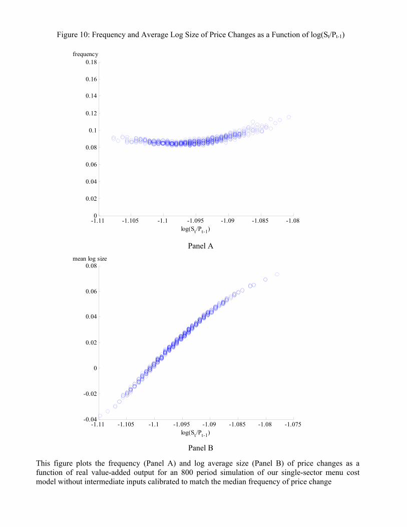
Figure 10: Frequency and Average Log Size of Price Changes as a Function of log(St/Pt-1)

Panel A

Panel B

This figure plots the frequency (Panel A) and log average size (Panel B) of price changes as a function of real value-added output for an 800 period simulation of our single-sector menu cost model without intermediate inputs calibrated to match the median frequency of price change

-1.11 -1.105 -1.1 -1.095 -1.09 -1.085 -1.080

0.02

0.04

0.06

0.08

0.1

0.12

0.14

0.16

0.18

log(St/Pt-1)

frequency

-1.11 -1.105 -1.1 -1.095 -1.09 -1.085 -1.08 -1.075-0.04

-0.02

0

0.02

0.04

0.06

0.08

log(St/Pt-1)

mean log size

Figure 11: CIR as a Function of the Expected Duration of Price Spells This figure presents the cumulative impulse response (CIR) of value-added output as a function of the expected duration of price spells in the single-sector menu cost model with intermediate inputs. The variance of the idiosyncratic shock is set equal to 0.0425 and the menu cost parameter is varied.

0

0.02

0.04

0.06

0.08

0.1

0.12

0.14

0 5 10 15 20 25 30 35 40Expected Duration (months)

CIR

Figure 12: Variance of Output as a Function of the Frequency of Price Change

This figure plots the variance of value-added output as a function of the frequency of price change for two calibrations of our single sector model without intermediate inputs. First, we present our benchmark calibration of μ=0.002, ση=0.0037 and σε=0.0425. Second, we present a calibration in which μ=0.01, ση=0.0037 and σε=0.01.

0

0.02

0.04

0.06

0.08

0.1

0.12

0.14

0 0.1 0.2 0.3 0.4 0.5 0.6Frequency

Variance of Output (10-4)

Pi=0.002, sigma_eps=0.0425

Pi=0.01, sigma_eps=0.01

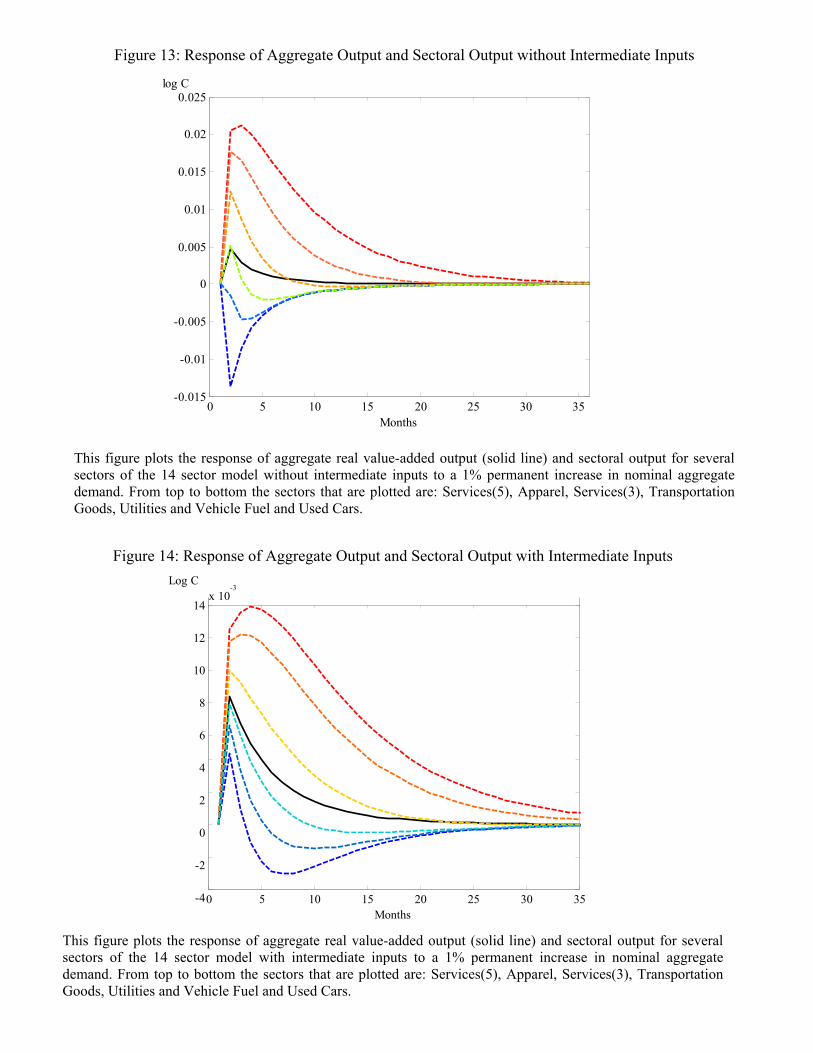
Figure 13: Response of Aggregate Output and Sectoral Output without Intermediate Inputs This figure plots the response of aggregate real value-added output (solid line) and sectoral output for several sectors of the 14 sector model without intermediate inputs to a 1% permanent increase in nominal aggregate demand. From top to bottom the sectors that are plotted are: Services(5), Apparel, Services(3), Transportation Goods, Utilities and Vehicle Fuel and Used Cars.

0 5 10 15 20 25 30 35-0.015

-0.01

-0.005

0

0.005

0.01

0.015

0.02

0.025

Months

log C

Figure 14: Response of Aggregate Output and Sectoral Output with Intermediate Inputs This figure plots the response of aggregate real value-added output (solid line) and sectoral output for several sectors of the 14 sector model with intermediate inputs to a 1% permanent increase in nominal aggregate demand. From top to bottom the sectors that are plotted are: Services(5), Apparel, Services(3), Transportation Goods, Utilities and Vehicle Fuel and Used Cars.

0 5 10 15 20 25 30 35-4

-2

0

2

4

6

8

10

12

14x 10

-3

Months

Log C

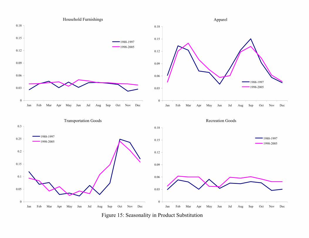
Figure 15: Seasonality in Product Substitution

Household Furnishings

0

0.03

0.06

0.09

0.12

0.15

0.18

Jan Feb Mar Apr May Jun Jul Aug Sep Oct Nov Dec

1988-19971998-2005

Apparel

0

0.03

0.06

0.09

0.12

0.15

0.18

Jan Feb Mar Apr May Jun Jul Aug Sep Oct Nov Dec

1988-19971998-2005

Transportation Goods

0

0.05

0.1

0.15

0.2

0.25

0.3

Jan Feb Mar Apr May Jun Jul Aug Sep Oct Nov Dec

1988-19971998-2005

Recreation Goods

0

0.03

0.06

0.09

0.12

0.15

0.18

Jan Feb Mar Apr May Jun Jul Aug Sep Oct Nov Dec

1988-19971998-2005