Price Rigidity and Monetary Non-Neutrality in Developing Countries: Evidence from Nigeria

International Journal of Economics and Financial Issues Vol. 3, No. 2, 2013, pp.525-536 ISSN: 2146-4138 www.econjournals.com

525

Price Rigidity and Monetary Non-Neutrality in Developing Countries:

Evidence from Nigeria

Nathaniel E. Urama Department of Economics, University Reading, Reading, UK;

Department of Economics, University of Nigeria, Nsukka, Nigeria. Email: [email protected]

Moses O. Oduh

Debt Management Office (DMO), The Presidency, Abuja, Nigeria. Email: [email protected]

Emmanuel O. Nwosu Department of Economics, University of Nigeria, Nsukka, Nigeria

Email: [email protected]

Augustine C. Odo

Godfrey Okeye University, Enugu, Nigeria. Email: [email protected]

ABSTRACT: In an attempt to find out the degree of monetary non-neutrality in Nigeria we started from finding out the size of price rigidity in the country. Computation with Ball and Romer method showed that price rigidity is optimal decision for firms in Nigeria only when the menu cost is well above 2.28% of the firm’s revenue which is on the high side, showing the likelihood of weak price rigidity in the country. Confirming this, the IRFs of the SVAR shows that the response of inflation to nominal shock has only one period lag. These combined results led to a small though persistent response of output to the nominal shock. The result of the study therefore points towards large nominal and small real effect of monetary policy in Nigeria and conclude that monetary policy will be a better option for contractionary plan but not for an expansionary plan. Keywords: Price rigidity; menu cost; monetary non-neutrality; monetary policy JEL Classifications: D40; E52; E63 1. Introduction

Monetary policy debate dates back to 1752 in David Hume’s work titled “Work of Money” where he presented the quantity theory of money. Through Say’s Law, he concluded that whatever is supplied in an economy will be purchased, leading to market clearing always (Snowdon and Vane, 2005:235). The implication of this is that money is neutral, affecting only the nominal variables but not the real variables in an economy, leading in turn to the classical dichotomy (that nominal variables do not affect real variables). As the classical belief could not explain the great depression of the 1930s, some economists including Keynes rose against it and explained that money is not neutral due to liquidity preferences. They explained that due to the fact that people will like to hold money back to facilitate transaction, maintain liquidity and for speculations, demand for money will not always equal to the supply and this led to the popular Keynes General Theory which is the origin of non-neutrality of money as it links monetary and real variables. Explaining the model further, Keynes replaced the constant velocity of money in the quantity theory with a fixed price-level. He said that an increase in expenditure that is not followed by an increase in price will create excess demand for goods, which increases the need for workers thereby, increasing employment and output. By implication, the statement implicitly tied the effectiveness of Keynes theory to price rigidity.

Price Rigidity and Monetary Non-Neutrality in Developing Countries: Evidence from Nigeria

526

This implied nominal rigidity and its implication on monetary non-neutrality have over the years, been gradually explained. Fisher (1977) explained the real impact of monetary policy on the bases of long term nominal wage contracts. As contained in Mankiw and Romer (1991: 6). J. B. Taylor extended the Fisher’s model by including staggered contracts and contracts that fixes nominal prices and wages as justification for monetary non-neutrality. Ball and Romer (1990), show that in addition to small friction in nominal adjustment, there is also real rigidity which in combination with the small nominal friction will create a significant nominal rigidity in an economy. Snowdon and Vane (2005:380-381) explains that real rigidity can arise when a firm is slow to change its price when there are changes to economic environment.

Though this argument has been on from the classical, through the Keynesian, Neo-classical, Neo-Keynesians, the New-Keynesian, to the New–Neoclassical, also called, New Synthesis, the only ‘conclusion’ is that in the short run, money is non-neutral but in the long-run, it is neutral. This means that Keynes theory works in the short run while the classical theory works in the long-run. To this end, most economies including the developing countries have adopted monetary policy as a means of regulating and stabilizing the economy based on the acclaimed short run non-neutrality of money due to sticky prices and wages, and market imperfections. 2. Problem Statement

Despite this general theoretical believe that monetary policy will helps in stabilizing economies at least in the short run, empirical findings and practical evidence have not been uniform. As contained in Hamid (2002), some of them totally reject the hypothesis of monetary neutrality, while others accept only the short run non-neutrality. Chuku (2009) has it that the actual effect of monetary policy shock on prices and output has been highly idiosyncratic. This may be linked to the fact that the impact of monetary policy in an economy depends on the size of the nominal rigidity which is in turn determined by some other variables that vary across countries and regions. According to Hamid (2002) these variables includes but not limited to menu cost, real price and wage rigidity, perfect capital market, and fixed nominal cost. Empirical evidence confirming the country specific nature of these variables especially price rigidity abounds (Dixon and Zhou, 2010; Nakamuru and Steinssion, 2008; Hoffman and Kuz-Kim, 2005; Vilmunen and Laakkonen, 2005 Veronese et al, 2005). In addition, some of them are totally lacking in developing countries, reducing nominal rigidity and casting doubt on the effectiveness of monetary policy in the region.

Of particular interest is the issue of price rigidity which as generally believed is the main factor that ensures non-neutrality of money and is brought about mainly by the cost of changing the price menu. In developing countries like Nigeria, most market for goods and services even in the most developed area of the country like Abuja and Lagos hardly make use of price tag which mostly contribute to the cost of changing the price menu. Most of the transactions are carried out through bargaining and negotiation. The so called price menu is just a hand written list of goods and their minimum prices for large shops with many sales agents or applicants. It is just of recent that few shops referred to as super-markets with the standard price menu started surfacing in the country. Presently however, their number is so minimal compared to the whole market. The menu cost, if applicable, is hence very negligible. Though Akerlof and Yellen (1985) are of the opinion that despite being small, the menu cost can still generate large nominal rigidity, Ball and Romer (1990) showed that this holds only for very high elasticity of labour supply. Because of high unemployment in the development countries, the elasticity of labour supply is very small and this casts even more doubt on the strength of nominal rigidity in the country.

The above ambiguity and country specific monetary impact calls for further research on the strength of nominal rigidity in the developing countries and that is what this particular study wants to pursue, using Nigeria as a case study. The need for the study is also clear from the statement of Ball and Romer (1990) that, though there are real rigidities, but in the absence of independent source of nominal stickiness, prices adjust fully to nominal shock, thereby counteracting the monetary non-neutrality of monetary shock theory.

Specifically therefore, this study intends to find out the size of the friction in nominal adjustment and then, the impact of monetary policy on both the nominal and real variables in Nigeria.

International Journal of Economics and Financial Issues, Vol. 3, No. 2, 2013, pp.525-536

527

The specific questions answered by the study are: 1. Is the size of the friction to nominal adjustment in Nigeria large enough to generate nominal

rigidity? 2. Is monetary policy in Nigeria just a pass through to nominal variables or does it have a real

impact?

3. Some Previous Empirical findings Using aggregate data, Dhyne et al. (2006) show that prices in the Euro area tends to remain

unchanged on average for 10.6 months. In UK, Hall et al. (2000) using data from the Bank of England survey in 1995, from 654 UK companies show that firms on average review their prices every month but changes it only twice in a year. Hoeberichts and Stokman (2006) show that price setting behaviour in Netherland depends critically on both a firm's size and the competitive environment it faces, and that wholesale and retail price are more flexible than those for business-to-business services.

In USA, Kashyap (1995) finds that prices stay fixed for several years before changing. Bils and Klenow (2004), however argues that the observed high price rigidity may be a result of using sample of very few commodities. They therefore used data on 350 products from the US retail price index on a monthly frequency and found a higher frequency of adjustment of 4.3 months. In Germany, Weber and Anders (2007) using data on meat products found that the prices of meat products such as beef can remain unchanged for up to 63 weeks. Chakrabarti and Scholnick (2007), also show high price rigidity for online book sellers. In France, Claire and Roland (2004) reports that prices are found to adjust infrequently, that the median firm reviews its price quarterly but modifies its price only once a year.

Roland et al. (2011) used micro data on price record to provide a detailed assessment of consumer price rigidity in Barbados. They find that prices in Barbados tend to change relatively frequently, with between 50 and 80 percent of items in every category reporting a price change every month. In Sierra Leone, Kovanen (2006), reports an average duration of price change of 2.6 months. Shinoz and Sarcoglu (2008) reports that in Turkey, median firms review their prices every month, but change their prices four times a year.

On the issue of effectiveness of monetary policy, Weeeks (2009) said, “the effectiveness of monetary policy depends on the values of the import share and the sum of the trade elasticities. Inspection of data from developing countries indicates the effectiveness of monetary policy under flexible exchange rates can be quite low even if capital flows are perfectly elastic”. In Nigeria, using cointegration and error correction mechanism, Ajisafe and Folorunso (2002) concludes that monetary policy exerts a greater influence on economic activities in Nigeria than fiscal policy. Using the same methods, Aigheyisi (2011) show that though both fiscal and monetary policies have positive impact on real GDP in Nigeria, the positive impact of monetary policy action are more significant than that of fiscal policy within the period covered by the study. On the other hand, Iyaji et al. (2012) reports that unethical banking practices by Nigerian commercial banks have rendered cash reserve ratio, broad money supply and exchange rate impotent resulting to ineffective monetary policy in Nigerian economy. Christiano et al. (1998) says that literature has not yet converged on a particular set of assumptions for identifying the effects of an exogenous shock to monetary policy. 4. Methodology 4.1 Model for Menu Cost and the Cost of Non-Adjustment

Answering the first question demands a model for the computation of the numerical values of the friction to price adjustment in Nigeria. For this, we will adopt the model used by Ball and Romer (1990). The assumptions of the model are as follows;

1. There is a continuum price setter agents uniformly distributed on [0,1]. 2. Each agent produces a differentiated goods with his labour as the only input, sales these goods

and purchases the goods of other agents. 3. There is imperfect competition in the market. 4. The agents’ profit depends on the real spending on the economy Y and on the relative prices

of the agent’s good iPP


528

5. There is a menu cost . Given the above assumptions, agent 'i s utility function is;

1i i i iU C L D

(1)

Where is the elasticity of substitution between any two goods, is the marginal disutility of labour, L is the agent’s labour supply, iD is a dummy variable for price adjustment with value of 1 if

the agent adjusts his price following a monetary shock and 0 otherwise. iC , measures the agents consumption and it is given as;

1

11

0i ij

j

C C dj

, for Cij equals the agent’s consumption of the product of agent j.

Assumption number two entails that the agent’s production function and output is given as i iY f L (2) Assuming agent i is a representative of all the agents in the economy, the relationship between aggregate output Y and real money balances M is given as YP M (3)

Where P is the Price index given as 1/ 11 1

0 iiP P di

(4)

A combination of the previous equations gives the demand for agent i’s product as

iyi

PMDdP P

(5)

The agent’s budget constraint together with this demand function transforms his utility into the form

1 1i i

i iP PM MU D

P P P P

(6)

The absence of menu cost and symmetric equilibrium prices 1,iP P i for a unique level of

M P , normalised to one, yields the utility of the form

, 1,1ii

PMUP P

(7)

According to Ball and Romer (1990), this assumption means that 2 1,1 0 , 22 1,1 is

negative and 12 1,1 is positive, where π is a profit function. With the subscripts representing partial

derivatives, 22 1,1 is therefore the price setters second order condition, and 12 1,1 0 guarantees stability of the equilibrium. On the assumption that the money supply will be normalised to one, the frictionless equilibrium means that each of the agent will set his price equal to one. Any change in money supply after this point leaves the agent with two options; paying the menu cost and adjusting his price or not paying the menu cost and continuing with the previous price. If all the agents pay the menu cost and adjust their price in line with the shocks in money supply, there is perfect price flexibility in the system (frictionless economy) but if all the agents refuse to pay the menu cost and to adjust their prices, it means that there is extreme price rigidity in the system. The latter case makes non-adjustment of prices to be a Nash equilibrium condition. The degree of nominal rigidity is therefore determined by the range of the realisation of M for which non-adjustment of price leads to Nash equilibrium.


529

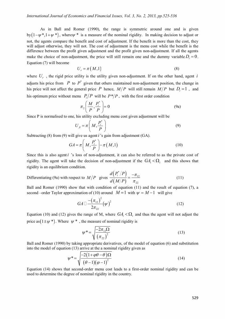
As in Ball and Romer (1990), the range is symmetric around one and is given by 1 *,1 * , where * is a measure of the nominal rigidity. In making decision to adjust or not, the agents compare the benefit and cost of adjustment. If the benefit is more than the cost, they will adjust otherwise, they will not. The cost of adjustment is the menu cost while the benefit is the difference between the profit given adjustment and the profit given non-adjustment. If all the agents make the choice of non-adjustment, the price will still remain one and the dummy variable 0iD . Equation (7) will become ,1rU M (8)

where rU , the rigid price utility is the utility given non-adjustment. If on the other hand, agent i

adjusts his price from P to *P given that others maintained non-adjustment position, the change in his price will not affect the general price P hence, M P will still remain M P but 1iD , and

his optimum price without menu iP P will be *P P , with the first order condition

*

2 , 0iPMP P

(9a)

Since P is normalised to one, his utility excluding menu cost given adjustment will be

*

, ifi

PU MP

(9)

Subtracting (8) from (9) will give us agent i ’s gain from adjustment (GA).

*

, ,1iPGA M MP

(10)

Since this is also agent i ’s loss of non-adjustment, it can also be referred to as the private cost of rigidity. The agent will take the decision of non-adjustment if the i iGA and this shows that rigidity is an equilibrium condition.

Differentiating (9a) with respect to M P gives

*12

22

id P Pd M P

(11)

Ball and Romer (1990) show that with condition of equation (11) and the result of equation (7), a second –order Taylor approximation of (10) around 1M with 1M will give

2212

222GA

(12)

Equation (10) and (12) gives the range of M, where i iGA and thus the agent will not adjust the

price as 1 * . Where * , the measure of nominal rigidity is

122

22

2*

(13)

Ball and Romer (1990) by taking appropriate derivatives, of the model of equation (6) and substitution into the model of equation (13) arrive at the a nominal rigidity given as

2

2 1*

1 1

(14)

Equation (14) shows that second-order menu cost leads to a first-order nominal rigidity and can be used to determine the degree of nominal rigidity in the country.


530

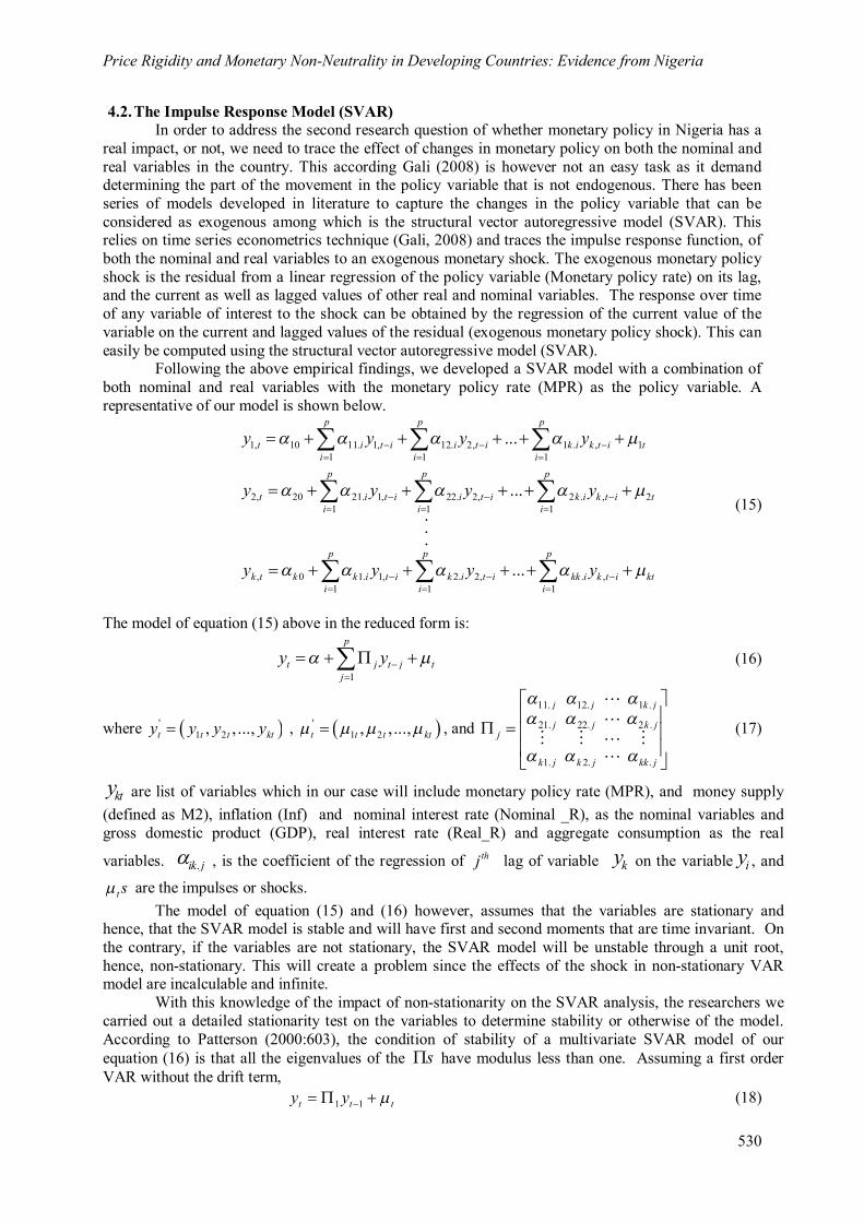
4.2. The Impulse Response Model (SVAR) In order to address the second research question of whether monetary policy in Nigeria has a

real impact, or not, we need to trace the effect of changes in monetary policy on both the nominal and real variables in the country. This according Gali (2008) is however not an easy task as it demand determining the part of the movement in the policy variable that is not endogenous. There has been series of models developed in literature to capture the changes in the policy variable that can be considered as exogenous among which is the structural vector autoregressive model (SVAR). This relies on time series econometrics technique (Gali, 2008) and traces the impulse response function, of both the nominal and real variables to an exogenous monetary shock. The exogenous monetary policy shock is the residual from a linear regression of the policy variable (Monetary policy rate) on its lag, and the current as well as lagged values of other real and nominal variables. The response over time of any variable of interest to the shock can be obtained by the regression of the current value of the variable on the current and lagged values of the residual (exogenous monetary policy shock). This can easily be computed using the structural vector autoregressive model (SVAR).

Following the above empirical findings, we developed a SVAR model with a combination of both nominal and real variables with the monetary policy rate (MPR) as the policy variable. A representative of our model is shown below.

1, 10 11. 1, 12. 2, 1 . , 11 1 1

2, 20 21. 1, 22. 2, 2 . , 21 1 1

...

... .

p p p

t i t i i t i k i k t i ti i i

p p p

t i t i i t i k i k t i ti i i

y y y y

y y y y

, 0 1. 1, 2. 2, . ,1 1 1

. .

...p p p

k t k k i t i k i t i kk i k t i kti i i

y y y y

(15)

The model of equation (15) above in the reduced form is:

1

p

t j t j tj

y y

(16)

where '1 2, , ...,t t t kty y y y , '

1 2, , ...,t t t kt , and 11. 12. 1 .

21. 22. 2 .

1. 2. .

j j k j

j j k jj

k j k j kk j

(17)

kty are list of variables which in our case will include monetary policy rate (MPR), and money supply (defined as M2), inflation (Inf) and nominal interest rate (Nominal _R), as the nominal variables and gross domestic product (GDP), real interest rate (Real_R) and aggregate consumption as the real

variables. .ik j , is the coefficient of the regression of thj lag of variable ky on the variable iy , and

t s are the impulses or shocks. The model of equation (15) and (16) however, assumes that the variables are stationary and

hence, that the SVAR model is stable and will have first and second moments that are time invariant. On the contrary, if the variables are not stationary, the SVAR model will be unstable through a unit root, hence, non-stationary. This will create a problem since the effects of the shock in non-stationary VAR model are incalculable and infinite.

With this knowledge of the impact of non-stationarity on the SVAR analysis, the researchers we carried out a detailed stationarity test on the variables to determine stability or otherwise of the model. According to Patterson (2000:603), the condition of stability of a multivariate SVAR model of our equation (16) is that all the eigenvalues of the s have modulus less than one. Assuming a first order VAR without the drift term, 1 1t t ty y (18)


531

It can be simplified to 1t tA L y (19)

With 11A L L as the autoregressive polynomial, we can obtain the eigenvalues of 1 by solving

the roots of the thk order characteristics polynomial equation given as 1 0I (20) Though equations (18), (19) and (20) are for first order SVAR, they are still applicable in our pth order SVAR model of equation (5) as our pth SVAR can be easily reformulated as a first order system by putting it in the companion form as: 0 1 1t t tY A AY (21) Equation (21) can thus be written in the format of (19) as: 0t tA L Y A (22)

with 1kpA L I A L , and kpI is the identity matrix of order x kp kp ; 1 1, ,..., 't t t t pY y y y ,

, 0,..., 0 'oA , , 0,..., 0 't t , and

1 2 1

1

1 0 0 00 1 0 00 0 0 0

0 0 0 1

p p

A

If from these stationarity tests, it is found that the variables of interest has unit root, which is likely the case from past experience and empirical evidences, we will have do an addition test for likely cointegration of the variables. If there is evidence of cointegration among the variables, it nullifies the effect of the unit root and we shall continue with our model of equation (16). Otherwise, we will have to reformulate the model in terms of the first, second and so on difference of the variables according the point at which they become stationary. Using ty as a representation of the variables, the first difference is given as, 1t t ty y y and our model of equation (16) will become

1

p

t j t j tj

y y

(23)

5. Results and Interpretation 5.1. Preliminary analysis

To avoid the ill impact of non stationarity in our result, we had to test the variables for stationarity. We used both the Philips-Peron and Augmented Dickey-Fuller unit root test and observed that none of the variables of interest is stationary at level. We tested for the stationarity of the first difference and found that most of their first difference is stationary at 5 or 10% level. This suggested the likelihood of cointegration which we tested and confirmed using the Johansen cointegration test. The result of the cointegration test shows that the variables despite being non-stationary individually, cointegrated at 5 per cent significant level. Thus, we went ahead with the normal model of equation (16) as the evidence of cointegration will remove the spuriousness that could have been caused by the presence of unit root (Gujarati, 2006; Hendry, 1995; and Patterson, 2000). 5.2. Price Rigidity in Nigeria

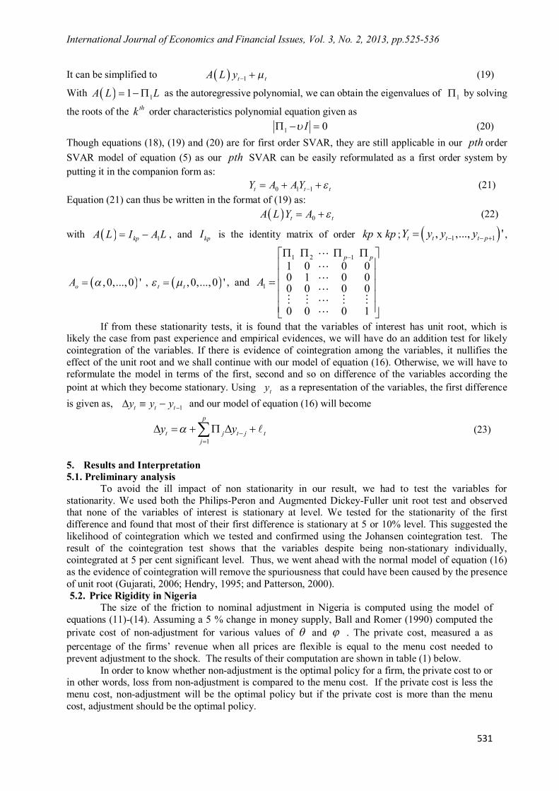
The size of the friction to nominal adjustment in Nigeria is computed using the model of equations (11)-(14). Assuming a 5 % change in money supply, Ball and Romer (1990) computed the private cost of non-adjustment for various values of and . The private cost, measured a as percentage of the firms’ revenue when all prices are flexible is equal to the menu cost needed to prevent adjustment to the shock. The results of their computation are shown in table (1) below.

In order to know whether non-adjustment is the optimal policy for a firm, the private cost to or in other words, loss from non-adjustment is compared to the menu cost. If the private cost is less the menu cost, non-adjustment will be the optimal policy but if the private cost is more than the menu cost, adjustment should be the optimal policy.


532

In order to link this to the Nigerian economy, we computed the elasticity of labour supply in the country using National Consumer Welfare Survey data conducted by the National Bureau of Statistics. We also computed the elasticity of demand for major products in Nigeria using data from a Market Survey conducted by African Institute for Applied Economics in the major trading cities in the country in 2011. The result shows a very low elasticity of labour supply of 0.034 and a high price elasticity of demand of 8.45. The low value of the labour supply elasticity can be linked to the high rate of unemployment in the country. This makes the labour supply non responsive to decreases in wage rate. On the other hand, the high demand elasticity of the goods can be linked to the fact that that most of the commodities are primary products with little differentiation. This makes for a high responsiveness of the demand of any firms product to a slight change in price. Table 1. Private cost on Non-adjustment to a 5% change in money supply

Table 1

Private Cost

Mark-up (1/(θ-1)

Labo

ur su

pply

el

astic

ity (1

/(ψ-1

) 5% 15% 50% 100%

0.05 2.28 2.16 1.64 1.22

0.15 0.79 0.71 0.53 0.39

0.5 0.23 0.2 0.14 0.1

1 0.11 0.1 0.06 0.04

The computed price elasticity of demand of 8.45 gives us a mark-up of 13.42%. When this and the labour supply elasticity value of 0.034 are substituted into the base line computed private cost of table (1), the private cost is more than 2.28% of the firm’s revenue. This means that for non-adjustment to be an optimal policy in reaction to a 5% increase in money supply, the menu cost for the firm must be greater than 2.28% of the firm’s revenue. This of course is a high value for menu cost that is not feasible especially in developing countries where most of the firms don’t operate with price menu but do their transactions through bargaining. 5.3. Dynamic response to a monetary shock.

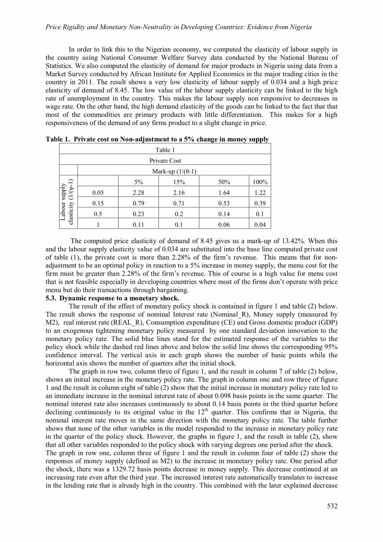
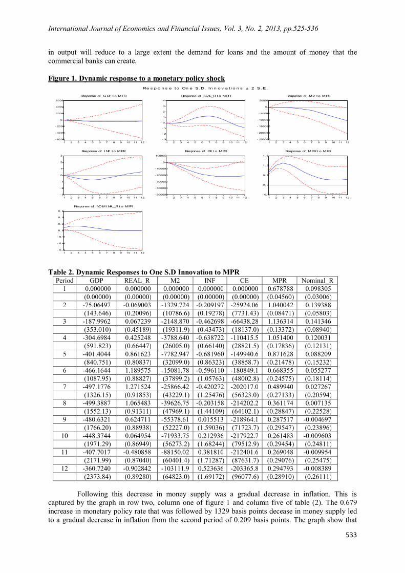
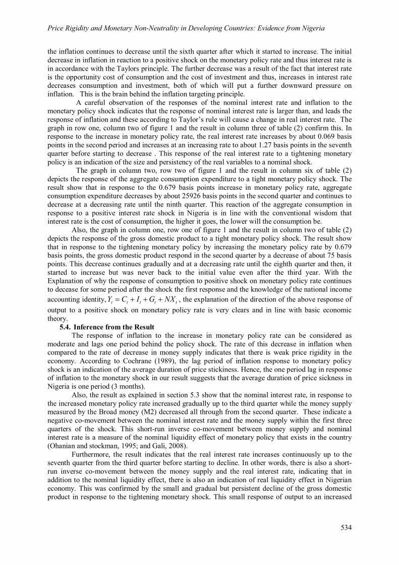
The result of the effect of monetary policy shock is contained in figure 1 and table (2) below. The result shows the response of nominal Interest rate (Nominal_R), Money supply (measured by M2), real interest rate (REAL_R), Consumption expenditure (CE) and Gross domestic product (GDP) to an exogenous tightening monetary policy measured by one standard deviation innovation to the monetary policy rate. The solid blue lines stand for the estimated response of the variables to the policy shock while the dashed red lines above and below the solid line shows the corresponding 95% confidence interval. The vertical axis in each graph shows the number of basic points while the horizontal axis shows the number of quarters after the initial shock.

The graph in row two, column three of figure 1, and the result in column 7 of table (2) below, shows an initial increase in the monetary policy rate. The graph in column one and row three of figure 1 and the result in column eight of table (2) show that the initial increase in monetary policy rate led to an immediate increase in the nominal interest rate of about 0.098 basis points in the same quarter. The nominal interest rate also increases continuously to about 0.14 basis points in the third quarter before declining continuously to its original value in the 12th quarter. This confirms that in Nigeria, the nominal interest rate moves in the same direction with the monetary policy rate. The table further shows that none of the other variables in the model responded to the increase in monetary policy rate in the quarter of the policy shock. However, the graphs in figure 1, and the result in table (2), show that all other variables responded to the policy shock with varying degrees one period after the shock. The graph in row one, column three of figure 1 and the result in column four of table (2) show the responses of money supply (defined as M2) to the increase in monetary policy rate. One period after the shock, there was a 1329.72 basis points decrease in money supply. This decrease continued at an increasing rate even after the third year. The increased interest rate automatically translates to increase in the lending rate that is already high in the country. This combined with the later explained decrease


533

in output will reduce to a large extent the demand for loans and the amount of money that the commercial banks can create.

Figure 1. Dynamic response to a monetary policy shock

- 6000

- 4000

- 2000

0

2000

4000

6000

1 2 3 4 5 6 7 8 9 10 11 12

Response of G DP t o M PR

- 3

- 2

- 1

0

1

2

3

4

1 2 3 4 5 6 7 8 9 10 11 12

Response of REAL_R t o MPR

- 250000

- 200000

- 150000

- 100000

- 50000

0

50000

1 2 3 4 5 6 7 8 9 10 11 12

Response of M2 t o MPR

- 3

- 2

- 1

0

1

2

3

1 2 3 4 5 6 7 8 9 10 11 12

Response of I NF t o MPR

- 500000

- 400000

- 300000

- 200000

- 100000

0

100000

1 2 3 4 5 6 7 8 9 10 11 12

Response of CE t o MPR

- 0. 5

0. 0

0. 5

1. 0

1. 5

1 2 3 4 5 6 7 8 9 10 11 12

Response of MPR t o MPR

- 0. 6

- 0. 4

- 0. 2

0. 0

0. 2

0. 4

0. 6

1 2 3 4 5 6 7 8 9 10 11 12

Response of NO MI NAL_R t o MPR

Re s p o n s e to On e S.D. In n o v a t i o n s ± 2 S .E.

Table 2. Dynamic Responses to One S.D Innovation to MPR

Period GDP REAL_R M2 INF CE MPR Nominal_R 1 0.000000 0.000000 0.000000 0.000000 0.000000 0.678788 0.098305 (0.00000) (0.00000) (0.00000) (0.00000) (0.00000) (0.04560) (0.03006) 2 -75.06497 -0.069003 -1329.724 -0.209197 -25924.06 1.040042 0.139388 (143.646) (0.20096) (10786.6) (0.19278) (7731.43) (0.08471) (0.05803) 3 -187.9962 0.067239 -2148.870 -0.462698 -66438.28 1.136314 0.141346 (353.010) (0.45189) (19311.9) (0.43473) (18137.0) (0.13372) (0.08940) 4 -304.6984 0.425248 -3788.640 -0.638722 -110415.5 1.051400 0.120031 (591.823) (0.66447) (26005.0) (0.66140) (28821.5) (0.17836) (0.12131) 5 -401.4044 0.861623 -7782.947 -0.681960 -149940.6 0.871628 0.088209 (840.751) (0.80837) (32099.0) (0.86323) (38858.7) (0.21478) (0.15232) 6 -466.1644 1.189575 -15081.78 -0.596110 -180849.1 0.668355 0.055277 (1087.95) (0.88827) (37899.2) (1.05763) (48002.8) (0.24575) (0.18114) 7 -497.1776 1.271524 -25866.42 -0.420272 -202017.0 0.489940 0.027267 (1326.15) (0.91853) (43229.1) (1.25476) (56323.0) (0.27133) (0.20594) 8 -499.3887 1.065483 -39626.75 -0.203158 -214202.2 0.361174 0.007135 (1552.13) (0.91311) (47969.1) (1.44109) (64102.1) (0.28847) (0.22528) 9 -480.6321 0.624711 -55378.61 0.015513 -218964.1 0.287517 -0.004697 (1766.20) (0.88938) (52227.0) (1.59036) (71723.7) (0.29547) (0.23896)

10 -448.3744 0.064954 -71933.75 0.212936 -217922.7 0.261483 -0.009603 (1971.29) (0.86949) (56273.2) (1.68244) (79512.9) (0.29454) (0.24811)

11 -407.7017 -0.480858 -88150.02 0.381810 -212401.6 0.269048 -0.009954 (2171.99) (0.87040) (60401.4) (1.71287) (87631.7) (0.29076) (0.25475)

12 -360.7240 -0.902842 -103111.9 0.523636 -203365.8 0.294793 -0.008389 (2373.84) (0.89280) (64823.0) (1.69172) (96077.6) (0.28910) (0.26111)

Following this decrease in money supply was a gradual decrease in inflation. This is captured by the graph in row two, column one of figure 1 and column five of table (2). The 0.679 increase in monetary policy rate that was followed by 1329 basis points decease in money supply led to a gradual decrease in inflation from the second period of 0.209 basis points. The graph show that


534

the inflation continues to decrease until the sixth quarter after which it started to increase. The initial decrease in inflation in reaction to a positive shock on the monetary policy rate and thus interest rate is in accordance with the Taylors principle. The further decrease was a result of the fact that interest rate is the opportunity cost of consumption and the cost of investment and thus, increases in interest rate decreases consumption and investment, both of which will put a further downward pressure on inflation. This is the brain behind the inflation targeting principle. A careful observation of the responses of the nominal interest rate and inflation to the monetary policy shock indicates that the response of nominal interest rate is larger than, and leads the response of inflation and these according to Taylor’s rule will cause a change in real interest rate. The graph in row one, column two of figure 1 and the result in column three of table (2) confirm this. In response to the increase in monetary policy rate, the real interest rate increases by about 0.069 basis points in the second period and increases at an increasing rate to about 1.27 basis points in the seventh quarter before starting to decrease . This response of the real interest rate to a tightening monetary policy is an indication of the size and persistency of the real variables to a nominal shock. The graph in column two, row two of figure 1 and the result in column six of table (2) depicts the response of the aggregate consumption expenditure to a tight monetary policy shock. The result show that in response to the 0.679 basis points increase in monetary policy rate, aggregate consumption expenditure decreases by about 25926 basis points in the second quarter and continues to decrease at a decreasing rate until the ninth quarter. This reaction of the aggregate consumption in response to a positive interest rate shock in Nigeria is in line with the conventional wisdom that interest rate is the cost of consumption, the higher it goes, the lower will the consumption be.

Also, the graph in column one, row one of figure 1 and the result in column two of table (2) depicts the response of the gross domestic product to a tight monetary policy shock. The result show that in response to the tightening monetary policy by increasing the monetary policy rate by 0.679 basis points, the gross domestic product respond in the second quarter by a decrease of about 75 basis points. This decrease continues gradually and at a decreasing rate until the eighth quarter and then, it started to increase but was never back to the initial value even after the third year. With the Explanation of why the response of consumption to positive shock on monetary policy rate continues to decease for some period after the shock the first response and the knowledge of the national income accounting identity, t t t t tY C I G NX , the explanation of the direction of the above response of output to a positive shock on monetary policy rate is very clears and in line with basic economic theory.

5.4. Inference from the Result The response of inflation to the increase in monetary policy rate can be considered as

moderate and lags one period behind the policy shock. The rate of this decrease in inflation when compared to the rate of decrease in money supply indicates that there is weak price rigidity in the economy. According to Cochrane (1989), the lag period of inflation response to monetary policy shock is an indication of the average duration of price stickiness. Hence, the one period lag in response of inflation to the monetary shock in our result suggests that the average duration of price sickness in Nigeria is one period (3 months).

Also, the result as explained in section 5.3 show that the nominal interest rate, in response to the increased monetary policy rate increased gradually up to the third quarter while the money supply measured by the Broad money (M2) decreased all through from the second quarter. These indicate a negative co-movement between the nominal interest rate and the money supply within the first three quarters of the shock. This short-run inverse co-movement between money supply and nominal interest rate is a measure of the nominal liquidity effect of monetary policy that exists in the country (Ohanian and stockman, 1995; and Gali, 2008).

Furthermore, the result indicates that the real interest rate increases continuously up to the seventh quarter from the third quarter before starting to decline. In other words, there is also a short-run inverse co-movement between the money supply and the real interest rate, indicating that in addition to the nominal liquidity effect, there is also an indication of real liquidity effect in Nigerian economy. This was confirmed by the small and gradual but persistent decline of the gross domestic product in response to the tightening monetary shock. This small response of output to an increased


535

monetary policy rate is observed by the Central bank of Nigeria monetary policy committee in the report of their Jan 2013 meeting (Central Bank of Nigeria, 2013). 6. Conclusion

From the result of both the computation of the cost of price rigidity and that of the impulse response of the inflation to changes in money supply, there is an indication of weak price rigidity in the country. The Computation using the Ball and Romer method showed that for price rigidity to be optimal decision for firms in Nigeria, the menu cost should be well above 2.28 percent of the firm’s revenue which is on the high side considering that most of the firms have a negligible menu cost. Confirming this, the impulse response function of the structural Vector Autoregressive model shows that inflation in Nigeria start responding to changes in money supply just one period after the change. These account for the small though persistent response of output to the nominal shock. These in other words, mean that there is a large nominal and small real effect of monetary policy in Nigeria. Even with this small real effect, Eric et al. (1996) is of the opinion that some of the noticed effects might have been a result of adverse supply shock and not that of changes in policy which he said will lead to understating the nominal impact and over stating the real impact.

The findings of the research have some important implications for economic policy decision in Nigeria. Since it reveals that monetary policies have more nominal than real effect in Nigeria, it then means that when the objective of the policy is contraction of nominal variables (inflation or nominal exchange rate) as is the case in Nigeria now with her inflation targeting objective, monetary policy will be a better option as it will have a large decreasing effect on inflation but a small decreasing effect on output. However, if the objective of the policy is expansionary (which is mostly of output), the result suggest that monetary policy may not be a better option as it will lead to large increase in inflation but a minute increase in output. References Aigheyisi, O.S. (2011), Examining the Relative Effectiveness of Monetary and Fiscal Policies in

Nigeria. A cointegration and error correction approach, http://ssrn.com/abstract=1944585 Ajisafe, R.A., Folorunso, B.A. (2002), The Relative Effectiveness of Fiscal and Monetary Policy in

Macroeconomic Management in Nigeria, The African Economic and Business Review, 3(1), 23-40.

Akerlof, G.A., Yellen, J.L. (1985), A Near-Rational Model of the Business Cycle, with the Wage and Price Inflation, Quarterly Journal of Economics, 100, 823-838.

Ball, L., Romer, D. (1990), Real Rigidity and Non-Neutrality of Money, Review of Economic Studies 57(2), 183-203.

Bils, M., Klenow, P.J. (2004), Some Evidence on the Importance of Sticky Prices, Journal of Political Economy, 112(5), 947-985.

Central Bank of Nigeria (2013), Communiqué No. 87 of the Monetary Policy Committee Meeting, Monday, January 21, 2013.

Chakrabarti, R., Scholnick, B. (2007), The Mechanics of Price Adjustment: New Evidence on the (Un) Importance of Menu Costs, Managerial and Decision Economics, 28, 657-668.

Christiano, LJ., Eichenbaum, M., Evan, C.L. (1998), Monetary Policy Shocks: What Have We Learned And To What End? NBER Working Paper 6400.

Chuku, A.C. (2009), Measuring the Effects of Monetary Policy Innovations in Nigeria: A Structural Vector Autoregressive (SVAR) Approach, African Journal of Accounting, Economics, Finance and Banking Research, 5(5), 112-129.

Claire, L., Roland, R. (2004), Price setting in France: new Evidence from survey data, Working Paper Series No. 423 / December 2004, European Central Bank.

Cochrane J. H. (1989), The Return of the Liquidity Effect: A Study of the Short-run Relationship between Money Growth and Interest Rate, Journal of Business and Economics Statistics, 7(1), 75-83.

Dhyne, E., Álvarez, L.J., Hoeberichts, M.M., Kwapil, C., Bihan, H., Lünnemann, P., Matins, F., Sabbatini, R., Stahl, H., Vermeulen, P., Vilmunen, J. (2006), Price Changes in the Euro Area and the United States: Some Facts from Individual Consumer Price Data, Journal of Economic Perspectives, 20(2), 171-192.


536

Dixon, H., Zhou, P. (2010), An Empirical Study on Price Rigidity, Cardiff Business School Working paper.

Eric, M.L., Sims, C.A., Zha, T. (1996), What Does Monetary Policy Do? Brookings Papers on Economic Activity, Brookings Institution.

Fischer, S. (1977), Long-Term Contracts, Rational Expectations, and the Optimal Money Supply Rule, The Journal of Political Economy 85(1), 191–205.

Hall, S., Walsh, M., Yates, A. (2000), Are UK Companies’ Price Sticky? Oxford Economic Papers, 52(3), p.425.

Gali, J. (2008), Monetary Policy, Inflation and the Business Cycle, Princeton University Press, New Jersey.

Gujarati, D.N. (2006), Basic Econometrics, Fourth Edition, Tata MacGraw-Hill, New york. Hamid, A. (2002), Testing The Long-run Neutrality of Money based on the Cointegration Theory: The

case of Iran, Iranian Economic Review, 6(6), 6-23. Hendry, D.F. (1995), Dynamic Econometrics, Oxford University Press, United State. Hoeberichts, M., Stokman, A. (2006), Price Setting Behaviour in the Netherlands: Results of a Survey,

Working Paper Series No 607 / April 2006, European Central Bank. Hoffmann, J., Kurz-Kim, J.R. (2005), Consumer Price Adjustment under the Microscope: Germany in

a period of Low Inflation. Deutsche Bundesbank, mimeo. Iyaji D., Success M.J., Success E.B. (2012), An assessment of the effectiveness of monetary policy in

combating inflation pressure on the Nigerian economy, Erudite Journal of Business Administration and Management, 1(1), 7-16.

Kashyap, A. K. (1995), Sticky Prices: New Evidence from Retail Catalogues, Quarterly Journal of Economic 110, 245-274.

Kovanen, A. (2006), What Do Prices in Sierra Leone Change So Often? A Case Study Using Micro-Level Price Data, IMF Working Paper WP/06/53, International Monetary Fund, Washington, DC.

Mankiew, N.G., Romer, D. (1991), New Keynesian Economics, Cambridge Mass: MIT Press. Nakamura, E., Steinsson, J. (2008), Five Facts about Prices: a Re-Evaluation of Menu Cost Models,

Quarterly Journal of Economics, 123(4), 1415-1464. Ohanian, L.E., Stochman, A.C. (19195), Theoretical Issues of Liquidity Effects, Review, May/June

1995. Patterson, K. (2000), An Introduction to Applied Econometrics: a time series approach, Palgrave,

New York. Roland C., Winston M., DeLisle W. (2011), Does Consumer Price Rigidity Exist in Barbados? Munich

Personal RePEc Archive, MPRA Paper No. 40928, posted 31. August 2012 15:01 UTC Sahinoz, S., Saracoglu, B. (2008), Price-setting Behaviour in Turkish Industries: Evidence from

Survey Data, The Developing Economies XLM (4), 363-85. Snowdon, B., Vane, H. (2005), Modern Macroeconomics, Cheltenham, UK: Edward Elgar ISBN 978-

1-84542-208-0. P.235. Veronese, G., Fabiani, S., Gattulli, A., Sabbatini, R. (2005), Consumer Price Behaviour in Italy:

Evidence from Micro CPI Data, ECB Working Paper, No. 449. Vilmunen, J., Laakkonen, H. (2005), How often do Prices Change in Finland? Evidence from Micro

CPI Data, Suomen Pankki, mimeo. Weber, S.A., Anders, S.M. (2007), Price Rigidity and Market Power in German Retailing, Managerial

and Decision Economics, 28, 737-749. Weeeks, J. (2009), The Effectiveness of Monetary Policy Reconsidered, Working Paper Series

Number 202, Political Economy research Institute.

Price Rigidity and Monetary Non-Neutrality in Developing Countries: Evidence from Nigeria

Documents

Transcript of Price Rigidity and Monetary Non-Neutrality in Developing Countries: Evidence from Nigeria