Hong Kong Monetary Authority

May 2004

ALTERNATIVE MEASURES OF CORE INFLATION ON THE MAINLAND

Key points:

• Concerns have recently risen about the pace with which inflationarypressures have been building up on the Mainland. An examination ofsectoral price movements reveals that upward pressures largely comefrom food prices.

• The question has been raised as to whether the headline inflation is agood indicator of “underlying” inflation – also referred to as “core”inflation. An adequate core inflation measure removes the impact oftransient shocks, and permits the analysis to be focused on morepersistent developments that are of greater relevance to monetary policy.

• This paper constructs several measures of core inflation with a view toproviding an indicator of underlying inflationary pressures on theMainland. Of the different measures, an Edgeworth index, which assignssmaller weights to the more volatile CPI components, is moreinformative for forecasting future inflation.

• This preferred core measure suggests that inflation pressures have beenmore subdued than signalled by the headline inflation rate. Nevertheless,these results need to be interpreted with caution as even this preferredcore inflation measure contains limited information useful forforecasting the headline inflation.

Prepared by : Chang Shu and Andrew TsangEconomic Research DivisionResearch DepartmentHong Kong Monetary Authority

- 2 -

I. Introduction

Monetary conditions and economic developments morebroadly in the Mainland are of central importance for Hong Kong’seconomic outlook. Given the close economic ties between the two regions,a return of inflation and accelerated growth on the Mainland may help liftHong Kong out of deflation. On the other hand, sharp swings inmacroeconomic conditions on the Mainland could deter economic growthin Hong Kong.

Price developments on the Mainland are clearly at a turningpoint. In early 2003, it was considered to be positive that the Mainlandseemed to experience modest rises in prices. However, the pace of priceincreases has accelerated since last August to a headline inflation rate of3.0% in March, 2004 (Chart 1). Concerns have been raised about the pacewith which inflationary pressures have been building up, and over whetherthe economy is overheating.

A close examination of price changes in different sectorsreveals that inflationary pressures have largely come from increases infood prices, which have been rising at a rate of more than 5% since lastOctober. Closely related to higher food prices, inflation has also beenhigher in rural than urban areas, in part reflecting a larger weight of foodin rural areas’ consumption basket (Chart 1).

These observations raise the question of whether the headlinerate accurately reflects the underlying trend in inflation. It is widelyrecognised that headline inflation contains a great deal of short-term noise,and various economic developments beyond the control of the central bankmay cause transitory changes in the inflation rate.1 Since it takes time forinflation to respond to monetary policy, central banks need to take a viewon the future evolution of inflation. Thus, what is more useful from apolicy point of view is to decompose headline inflation into a transientcomponent on the one hand, and a trend component – referred to as “core”inflation – reflecting persisting sources of inflation pressures on the other.

1 Transitory shocks to prices may be caused by factors such as changes in administratively set prices,

taxes, weather and oil supply.

- 3 -

It is the latter component that contains the most relevant information froma central bank’s perspective. If price fluctuations from non-monetarysources are effectively removed from the headline inflation, the resultingcore inflation can be regarded as the outcome of monetary policy.

A useful core inflation measure can be calculated in real time,that is, using contemporaneously available data. It contains informationuseful for forecasting changes in inflation in coming periods, whileminimising misleading signals about current and future trends in inflation.It should also be easily understood by the general public.

Many different core measures have been applied to studyunderlying inflation in industrial economies. There are, however, fewstudies that have investigated core inflation in Hong Kong and theMainland. Fan (2001) compares a number of core measures for HongKong, and concludes that the headline inflation rate is a good indicator ofunderlying pressures. Gerlach and Yiu (2004) use a statistical method toderive a core inflation measure for Hong Kong and the Mainland.

This paper calculates a number of core inflation measures forthe Mainland using alternative approaches, and evaluates theirperformance in gauging inflationary pressures. The rest of the paper isorganised as follows. Section II reviews the price development in theMainland in the last ten years, particularly the current inflation episode.Section III discusses different approaches in estimating core inflation,focusing on the measures that will be applied in this study. Section IVderives a number of core inflation measures for the Mainland, whileSection V considers whether these are good indictors of underlyinginflation. The analysis suggests that an Edgeworth index, which assignssmaller weights to more volatile CPI components, contains moreinformation useful for forecasting future inflation. According to thisindicator, inflation pressures have been more subdued than signalled by theheadline rate. Applying the same measures, Section VI finds that coreinflation in rural areas is around two percentage points higher than inurban areas. Finally, Section VII assesses the inflation outlook for theMainland.

- 4 -

II. Price Developments on the Mainland

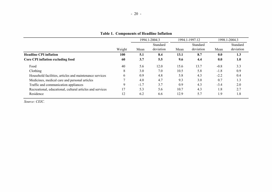
Price developments on the Mainland in the last decade can bedivided into two periods (Chart 1 and Table 1). The first was between1994 and 1997 during which the economy underwent sharp disinflation,with the inflation rate falling from over 20% at the beginning of the periodto around 3% at the end of 1997. The inflation rate has been much lowersince 1998, and the economy has also experienced sporadic deflation.Fluctuations in inflation have also been smaller. An important question iswhether the recent pick-up in inflation represents a distinct upturn in theinflation cycle.

An examination of the components of the CPI basket revealsthat food has the largest weight, accounting for around 40% ofconsumption expenditure. Yet it was a relatively more volatile item,falling from an average inflation rate of 15.6% per annum before 1998 to1.0% deflation after 1998.

In the current inflation episode, food has been the key drivingforce with prices rising by close to an annual rate of 10% since lastNovember – a rate only seen during the high inflation period in the early1990s. Housing costs also saw notable increases in the last few months.Upward pressures on prices of other consumption items have been moresubdued. In particular, two categories – household facilities, articles andmaintenance services; and traffic and communication appliances – haveseen the largest price falls in recent years, and their prices are stilldeclining at an annual rate of around 2%.

Price developments in urban and rural areas have followedbroadly the same trend (Chart 1). However, inflation has in general beenhigher in rural than urban areas since September 2001. Notably, theinflation differential between the two regions has risen in the currentepisode to almost two percentage points in the first two months of 2004.This is probably closely related to a more rapid rise in food prices.Section VI will examine in more details causes of this widening pricedifferential between the two regions.

- 5 -

III. A Review of Core Inflation Measures

Central banks and academics have carried out extensive workon developing good measures of core inflation. Broadly speaking, thereare three approaches – structural, exclusion-based and statistical. Thestructural approach draws a direct link between policy and core inflation,defining the latter as the inflation that is controllable through monetarypolicy, e.g. Quah and Vahey (1995), Blix (1995), Bjornland (1997) andClaus (1997). The difficulty with it, however, is that the resulting measureof core inflation tends to be sensitive to the assumptions underlying themodel, and the arrival of new data will result in a change in the historicalcore inflation series produced by the model. This makes it difficult toexplain to the general public and can undermine credibility of monetarypolicy. As the name suggests, the exclusion-based approach excludescertain items from the aggregate inflation in order to remove the influenceof unrepresentative price movements. The final approach often usesformal statistical methods to construct core inflation measures.

This paper applies the last two approaches to derive five coremeasures. The remainder of this section will briefly discuss the rationalesbehind these measures.

The exclusion-based approach: CPI excluding food and energy

This is the most commonly used method for assessingunderlying inflation. The Bureau of Labor Statistics in the United Statescomputes a core inflation measure that consists of a weighted average ofall CPI components except for food and energy. The rationale forexclusion is that food and energy are subject to large, short-term variationsdue to factors such as weather and oil supply. Many of the variations aredriven by non-monetary factors, and can be quickly reversed. As such,food and energy prices do not necessarily convey much useful informationabout underlying price trends.

- 6 -

One issue with exclusion-based measures is that they mightdiscard potentially useful information about core inflation that may becontained in food and energy prices or whatever categories that areexcluded. This concern is particularly significant for less developedeconomies such as the Mainland where food tends to have a much largerweight in the CPI basket than in advanced economies. They are furthersubject to the shortcoming that a once-and-for-all judgement has to bemade about what prices can be ignored in calculating core inflation.

Principal component analysis

Principal component analysis is a statistical method thatexplains variations of a group of variables (in this case the differentcomponents of a price index) by summarising them into a number offactors – referred to as principal components. It is often found that a largefraction of the original variables’ variations is explained by the firstprincipal component, which is then said to represent the most interestingdynamics of these variables. The details of principal component analysiscan be found in the Technical Appendix.

Exponential smoothing

Exponential smoothing is a method which forecasts thecurrent value of a variable by taking a weighted average of its past values.Cogley (2002) applies it to the US data, and shows that it outperformsother core measures in filtering out transient shocks and in focusing onmore persistent movements in inflation. This measure tends to besmoother than other core indicators.

The Edgeworth index

The Edgeworth index is calculated by assigning smallerweights to the more volatile components of the CPI. The rationale is thatthe more variable CPI components are, the less useful they are insignalling the underlying price trend. Unlike the exclusion-based approach,this method down-weights relatively more volatile items instead of

- 7 -

eliminating them. Dow (1994), Diewert (1995) and Wynne (2001) haveestimated this type of indices for the US. Details of the Edgeworth indexare provided in the Technical Appendix.

One issue in deriving the Edgeworth index is that it involvesan arbitrary choice of a time period for calculating volatility. Somestudies use a full sample, which gives the index an unfair advantage whenevaluating its ability in tracking headline inflation in real time. One wayof overcoming this problem is to use only the past 12 months, for example,for calculation. This allows the weights to change over time as thevolatility of different categories of prices changes over time. The speedwith which the weights change in response to changes in volatility will bedetermined by the choice of the fixed number of periods in calculation.

IV. Application for the Mainland

Data

The National Bureau of Statistics of China publishes data onyear-on-year changes of CPI components both for the Mainland as a whole,and for urban and rural areas. However, disaggregate data are onlyavailable for seven major categories of consumption expenditure. Furtherbreakdown in a comprehensive manner is only published on an annualbasis, and hence cannot be used to derive indicators of underlying inflationon a timely basis. For constructing the exclusion-based CPI measure,weights for different CPI components are needed. These can be calculatedfrom data on disaggregate consumption expenditure. All the data areextracted from the CEIC.

As discussed earlier, price developments on the Mainland aredistinctly different in the periods before and after 1998. Our analysis willfocus on the second period of relatively stable inflation.2

2 From an econometric point, the inflation series appear to be locally mean-reverting during

this period, which alleviates the potential problem of spurious correlations.

- 8 -

Measures of core inflation for the Mainland

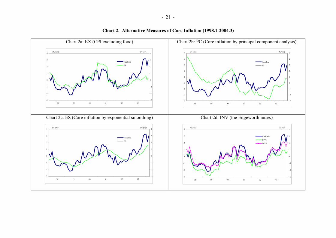
Based on the discussion in the previous section, a number ofcore inflation measures are derived (Charts 2a-d). The five measures are: a)CPI excluding food3 (EX); b) CPI extracted using principal componentanalysis (PC); c) CPI using exponential smoothing (ES); and d) twoEdgeworth measures (INV1 and INV2). The difference between the twoEdgeworth indices is explained later.

The five core inflation measures track the headline inflation todifferent degrees. An inspection of the plots of the different core inflationmeasures against the headline inflation suggests that PC deviates fromheadline inflation significantly, even though it averages out to have thesame mean as the latter (Chart 2b and Table 2). In fact it is the only coremeasure that is negatively correlated with the headline inflation (Table 3).It is more volatile than the headline inflation, and thus does not adequatelyreduce volatility.

EX is better at tracking the headline inflation with a positivecorrelation of 0.64 with the latter, and is also less volatile than theheadline measure.

In deriving the exponential smoothing measure (ES), adecision needs to be made on how quickly the influence of the past pricemovements dies down. The final ES measure adopted in this study iscalculated under the assumption that half of the adjustment will take placein 4 quarters. This is a plausible speed of adjustment, and the results arerobust to a range of assumptions with regard to the adjustment process. EShas a correlation of 0.74 with the headline inflation, as well as achieving areduction in volatility. Compared to the other core indicators, ES appearsto be particularly smooth.

3 There is no information on the energy component of the CPI in the Mainland.

- 9 -

The Edgeworth indices are derived using volatility calculatedbased on historical data. We have experimented with using the past 12, 18and 24 months for calculation, and found that the core measure obtainedfrom applying 12 months has the highest correlation with the headlineinflation. It may be because measures using too long a lag giveunwarranted influence to the pre-1998 period when inflation developmentswere distinctly different from the period after 1998.

Two Edgeworth measures are reported. INV1 uses all theseven major categories of the CPI for calculation. As can be seen inChart 2d, it is below the headline inflation for almost the whole post-1998period. A desirable property of a core inflation measure is that if theheadline inflation deviates from it, the headline should adjust to the coremeasure. The fact that INV1 is persistently below the headline measurewould imply that the latter always needs to adjust downward, which is notreasonable. The reason that INV1 is consistently lower is that the twoitems with the most rapidly falling prices – a) household facilities andservices; and b) traffic and communication appliances – are also relativelyless volatile, and thus are given more weights by construction incalculating this indicator. In an effort to overcome this problem, we derivea second Edgeworth index – INV2 – by excluding those two categories.These two categories account for only around 15% of total consumptionexpenditure, and thus their exclusion does not significantly reduce thecoverage of the resulting core measure.

A comparison of INV1 and INV2 shows that both are morestrongly correlated with the headline inflation, especially INV2, than othercore measures. Compared with other core measures, INV1 and INV2appear to strike a reasonable balance between having a high correlationwith the headline inflation and achieving a reduction in volatility.However, INV1 has a much lower mean than the headline and other coreinflation measures, reflecting the problem of a downward bias.

- 10 -

V. Evaluating Measures of Core Inflation

There are many criteria for evaluating how good core inflationmeasures are. Wynne (1999) lists a few, suggesting that core measuresshould:

• be able to be calculated in real time;• contains information useful for forecasting future changes in

inflation;• be easily understood by the public;• not change history when new observations are added; and• ideally have some theoretical basis.

In this section we evaluate the performance of the five coreinflation measures against some of these criteria.

Computable in real time

All the five indices derived above only use historical data, andthus can be calculated in real time.

Verifiable

The five measures are derived using formal statisticalmeasures. They can be verified by independent analysts, which canincrease the credibility of these measures in particular, and that ofmonetary policy conduct in general.

Forward looking

A good core inflation measure should be able to forecast themovement of the headline inflation in that deviations of the headlineinflation from the core measure should lead to the adjustment of theheadline towards the core, but not the reverse adjustment of the coretowards the headline. That is, we can run the following regressions:

- 11 -

(1) πt+h – πt = αh,h + βh,h(πt – core

tπ ) + ut+h,h,

(2) core

ht+π – core

tπ = αh,c + βh,c(πt – core

tπ ) + ut+h,c,

where:

πt+h : h-period-ahead headline inflationπt : headline inflation

core

ht+π : h-period-ahead core inflationcore

tπ : core inflation.

A core inflation measure is forward looking if Equation (1) has highexplanatory power while Equation (2) has little. This means that thewedge between πt and core

tπ is useful for forecasting future movements ofthe headline inflation, but not for those of core inflation.

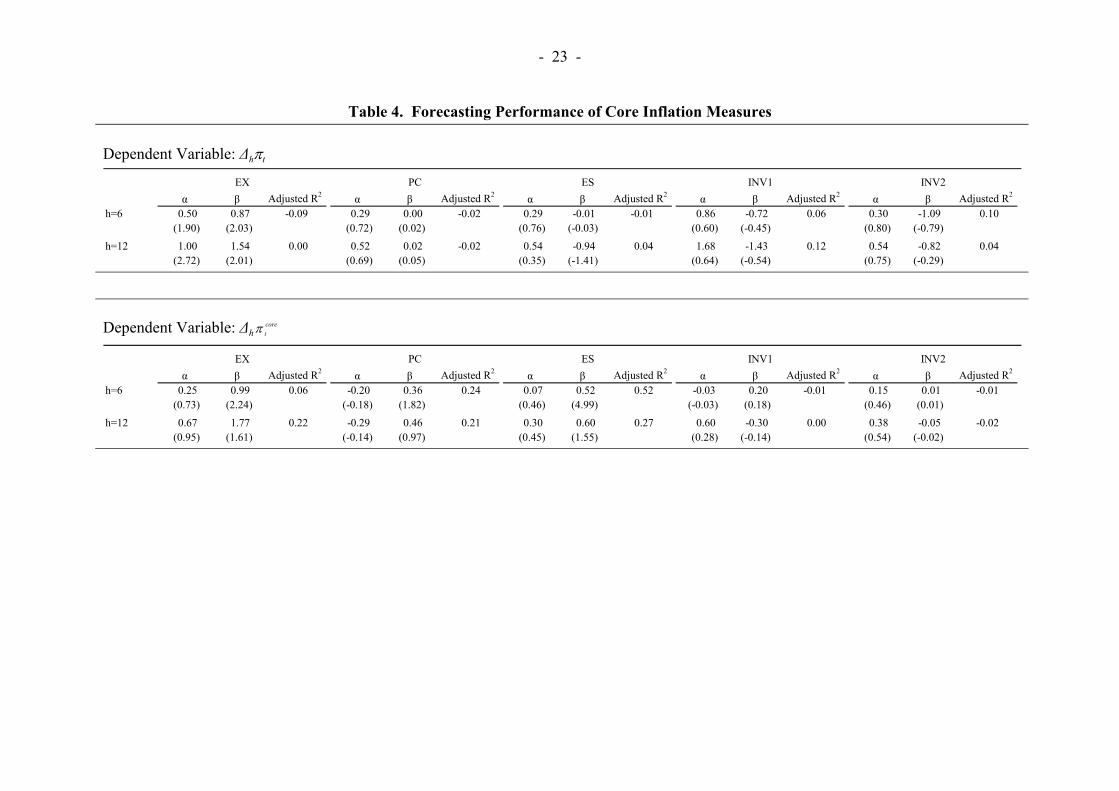
Table 4 reports the results of these regressions.4 The upperpanel of the table shows that EX and PC is not helpful for predicting theheadline inflation. ES has some predictive power over a 12-month horizon.The two Edgeworth indices can forecast the headline inflation as thewedge between the headline and core inflation rates causes the headline toadjust toward the core inflation, with INV1 doing marginally better overthe 12-month horizon and INV2 over the 6-month horizon. Nevertheless,they seem to contain little useful information about future movements ofthe headline inflation.

The lower panel of Table 4 shows that the first threemeasures – EX, PC and ES adjust toward the headline inflation, while thetwo Edgeworth indices do not.

4 The Generalised Method of Moments is used for estimation to deal with the simultaneity

issue, and the standard errors have been corrected for heteroskedasticity and autocorrelation.

- 12 -

Overall, results in this section suggest that INV2 is a bettercore inflation measure for the Mainland. It is highly correlated with theheadline inflation, and slightly more forward looking than the three non-Egdeworth core inflation measures. Nor does it suffer from the samedownward bias as INV1. According to INV2, inflation pressures are moresubdued than suggested by the headline inflation.

VI. Core Inflation in Urban and Rural Areas

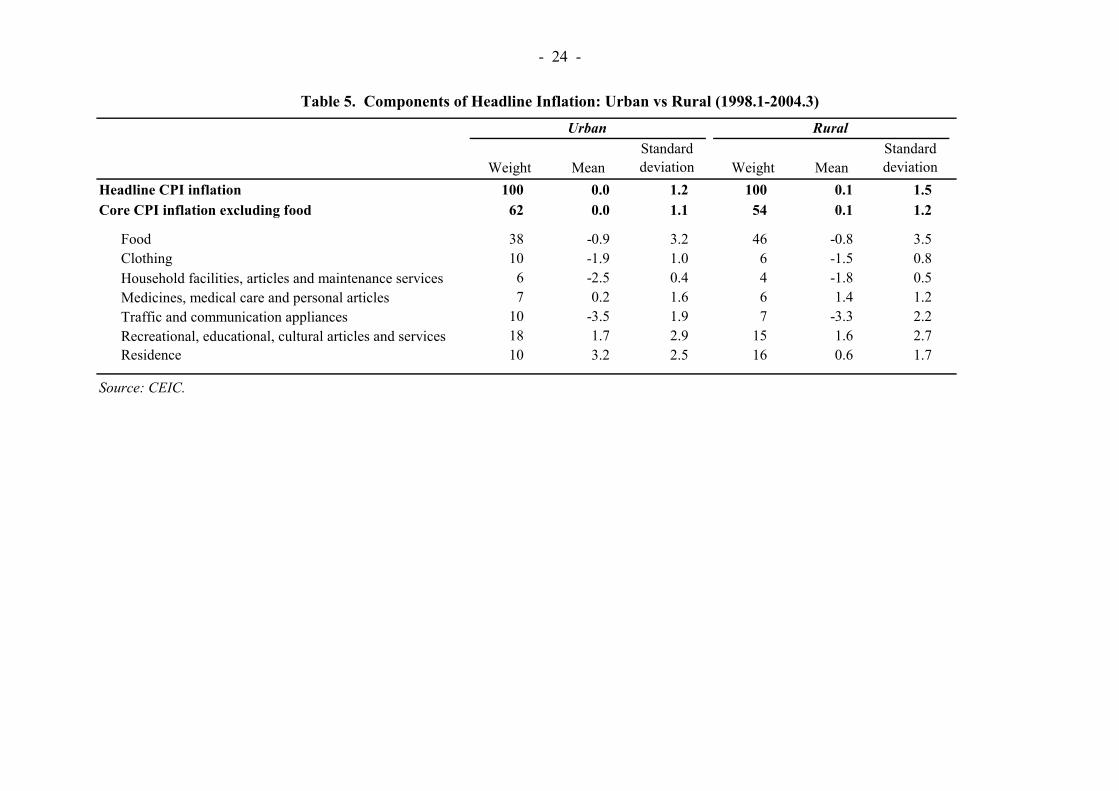
As noted above, inflation in rural areas has been higher thanin urban areas in recent years. A close examination of the breakdown ofconsumer prices shows that the prices of the two items – food and housingcosts – have been rising much faster in rural areas, especially since lastNovember. These two components account for a greater share inconsumption expenditure in rural areas, at 62% compared to 48% for urbanareas (Table 5). As a result, the inflation differential between rural andurban areas has risen in the past few months.

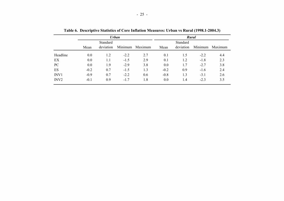
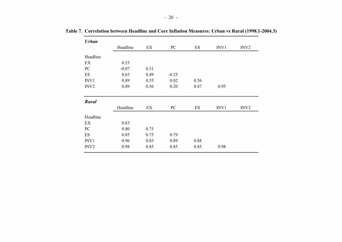
This section applies the same methods to assess underlyinginflation in rural and urban areas. The descriptive statistics of the fivecore measures reveal a similar pattern of the rural and urban core inflationmeasures as that of the nation-wide ones (Table 6). A few notableobservations are: a) PC for both regions has the same mean as the headlineinflation, but is more volatile; b) ES seems to be smoother than otherindicators; c) INV1 contains a large negative bias than others. There isone notable difference between rural and urban areas. Similar to thenation-wide measures, PC is not correlated with the headline inflation,while the two Edgeworth indices have high correlation in the case of urbanareas (Table 7). For rural areas, all the core measures are highly correlatedwith the headline inflation, including PC.

In testing the forward looking characteristics, Table 8 showsthat again the three non-Edgeworth indicators are very poor core measuresin that they are not able to predict future movements of the headlineinflation, but converge to the latter instead. The two Egdeworth indices

- 13 -

can forecast the urban headline inflation over both the 6- and 12-monthhorizon, and the predictive power is higher than in the case of nation-wideinflation. However, they are not useful in predicting the headline inflationin the case of rural areas by and large, except over the 6-month horizonusing INV2.

The analysis in this section suggests that the nation-wide pricedevelopments are dominated by those in urban areas, reflecting muchhigher average consumption in urban than rural areas. In 2003, the urbanpopulation was two thirds of the rural population, but average consumptionexpenditure in urban areas was more than three times that in rural areas.

Weighing the performance of the five core measures based ondifferent criteria, INV2 is probably the best for urban areas. It suggests amodest underlying inflation rate of around 1% at present.

INV2 is also a better measure of underlying inflation for ruralareas as it is highly correlated with the headline inflation and achieves areduction in volatility, but its weakness is that it contains little informationuseful for forecasting the headline inflation. Nevertheless, INV2 suggeststhat underlying inflation in rural areas is around two percentage pointshigher than in urban areas.

VII. Assessing Inflationary Pressures in the Mainland and the PolicyImplications

This paper has constructed a number of measures ofunderlying inflation on the Mainland in order to assess inflation pressuresin recent months. Of the five different core inflation measures derived, anEdgeworth index, which assigns smaller weights to the more volatile CPIcomponents, performs better than others in achieving a balance betweenhigh correlation with the headline inflation and a reduction in volatility.This measure suggests that inflation pressures are more subdued thanindicated by the headline inflation. Underlying inflation in rural areas isaround two percentage points higher than in urban areas at present.However, nation-wide price developments are dominated by those in urban

- 14 -

areas, reflecting higher urban consumption expenditure. Nevertheless,these results need to be interpreted with caution as even this preferred coreinflation measure contains limited information useful for forecasting futureheadline inflation, especially in the case of rural areas.

It is difficult to judge at this point how strongly inflation willrise in the coming periods. On the one hand, it can be argued thatinflationary pressures may well intensify. Increases in food prices andhousing costs raise the cost of living. This might lead to demand forhigher wages, triggering an upward spiral of wage and price adjustment.This, coupled with sharp rises in prices of raw materials as a result of fastinvestment growth, might eventually translate into higher general prices.On the other hand, however, upward wage pressures might be limited,given the large surplus labour on the Mainland. Separately, excessinvestment is likely to lead to over-capacity, restraining prices down theroad. Given the complexity of economic dynamics, it is important tomonitor a broad set of indicators in assessing the likely future path ofinflation, including price developments other than consumer prices, pass-through between different prices as well as both the demand and supplysides of the economy.

- 15 -

Summary of Core Inflation Measures

EX : CPI excluding foodPC : core inflation derived by principal component analysisES : core inflation derived by exponential smoothingINV1 : the Edgeworth index using all the seven major CPI componentsINV2 : the Edgeworth index using five CPI components, i.e. excluding:

a) household facilities and services; and b) traffic andcommunication appliances

- 16 -

References

Bjornland, Hilde C. (1997). Estimating core inflation- the role of oil price shocksand imported inflation. Statistics Norway Research Department DiscussionPaper, 200.

Blix, Marten (1995). Underlying inflation: a common trends approach. SverigesRiskbank Working Paper, 23.

Claus, Iris (1997). A measure of underlying inflation in the United States. Bank ofCanada Working Paper, 97-20.

Cogley, Timothy (2002). A simple adaptive measure of core inflation. Journal ofMoney, Credit, and Banking, 34(1), 94-113.

Diewert, W. Erwin (1995). On the stochastic approach to index numbers.University of British Columbia Department of Economics Discussion Paper,95/31.

Dow, James P., Jr. (1994). Measuring inflation using multiple price indexes.University of California-Riverside Department of Economics, unpublishedmanuscript.

Fan, Kelvin (2001). Measures of core inflation in Hong Kong. Hong KongMonetary Authority Research Memorandum,http://www.info.gov.hk/hkma/eng/research/RM14-2001_core_inflation.pdf.

Gerlach, Stefan and Matthew Yiu (2004). A simple measure of underlyinginflation: estimates for Hong Kong and the Mainland. Hong Kong MonetaryAuthority Research Memorandum,http://www.info.gov.hk/hkma/eng/research/RM02-2004.pdf.

Quah, Danny and Shaun P. Vahey (1995). Measuring core inflation. TheEconomic Journal, 105 (September), 1130-1144.

Vega, Juan-Luis and Mark A. Wynne (2001). An Evaluation of some measures ofcore inflation for the Euro Area. European Central Bank Working Paper, 53,April 2001.

Wynne, Mark A. (1999). Core inflation: A review of some conceptual issues.Federal Reserve Bank of Dallas Research Department Working Paper, 9903.

- 17 -

Technical Appendix

Principal component analysis

Principal component analysis is a commonly used non-parametricmethod for extracting relevant information from confusing data. Itattempts to explain the total variability of p correlated variables throughthe use of p orthogonal components, which are themselves weighted linearcombination of the original variables. Mathematically, define a randomvector:

(A.1)

=

p

2

1

X

XX

XM

.

The first principal component can be expressed as:

(A.2) pp XaXaXaY 12121111 ...+++= .

The ija are scaled such that 1' =11aa . 1Y is the linear combination thataccounts for the maximum variability of the p variables. Its variance is 1λ .

The second principal component 2Y is similarly formed, withadditional conditions that that its variance, 2λ , explains the maximumamount of the remaining variability of the p variables, and that 2Y isorthogonal to the first principal component, i.e. 02

' =aa1 .

Up to p principal components can be extracted in the same way.However, it is often found that the first k<p principal components explaina large fraction of the total variability of the p variables, and thus said thatthe most interesting dynamics occur in the first k dimensions.

The weights used to create the principal components are theeigenvectors of the characteristic equation:

(A.3) 0aIS i =− )( λ , or0aIR i =− )( λ ,

- 18 -

where S is the covariance matrix, and R is the correlation matrix. The iλ --variances of the components -- are the eigenvalues, and are obtained bysolving 0IS i =− λ .

The Edgeworth index

The Edgeworth index is obtained by re-weighting the CPIcomponents, using as weights the inverse of the volatility of the differencebetween the inflation rate of each CPI component and the headlineinflation rate. Both standard deviations and variances have been used asmeasures of volatility. If standard deviations are used, then:

(A.4) ∑=

=N

iititEdgeworth

1

πω ,

with:

∑=

=N

j jt

itit

1

1

1

σ

σω ,

1

)(1

2

−

−=∑

=

T

yyT

ji

itσ ,

titiy ππ −= ,

∑=

−=T

ititT

y1

)(1 ππ ,

for i=1, 2,…, N.

In the formula, tπ is the headline inflation, itπ the inflation rate of CPIcomponents, N the number of components, and T the number of timeperiods.

- 19 -

Chart 1. Headline Inflation (1994.1-2004.3)

-5

0

5

10

15

20

25

30(% yoy)

-5

0

5

10

15

20

25

30

94 95 96 97 98 99 00 01 02 03

(% yoy)

OverallUrbanRural

0

1

2

3

4

5

0

1

2

3

4

5

Jan Mar May Jul Sep Nov Jan Mar03 04

- 20 -

Table 1. Components of Headline Inflation

Weight MeanStandard deviation Mean

Standard deviation Mean

Standard deviation

Headline CPI inflation 100 5.1 8.4 13.1 8.7 0.0 1.3Core CPI inflation excluding food 60 3.7 5.5 9.6 4.4 0.0 1.0

Food 40 5.6 12.0 15.6 13.7 -0.8 3.3Clothing 8 3.0 7.0 10.5 5.8 -1.8 0.9

6 0.9 4.8 5.8 4.3 -2.2 0.47 4.0 4.7 9.3 3.0 0.7 1.39 -1.7 3.7 0.9 4.3 -3.4 2.0

17 5.3 5.6 10.7 4.3 1.8 2.7Residence 12 6.2 6.6 12.9 5.7 1.9 1.8

Source: CEIC.

Recreational, educational, cultural articles and services

1998.1-2004.3

Household facilities, articles and maintenance servicesMedicines, medical care and personal articlesTraffic and communication appliances

1994.1-2004.3 1994.1-1997.12

- 21 -

Chart 2. Alternative Measures of Core Inflation (1998.1-2004.3)

Chart 2a: EX (CPI excluding food) Chart 2b: PC (Core inflation by principal component analysis)

-3

-2

-1

0

1

2

3

4(% yoy)

-3

-2

-1

0

1

2

3

4

98 99 00 01 02 03

(% yoy)

Headline

EX

-3

-2

-1

0

1

2

3

4

5(% yoy)

-3

-2

-1

0

1

2

3

4

5

98 99 00 01 02 03

(% yoy)

Headline

PC

Chart 2c: ES (Core inflation by exponential smoothing) Chart 2d: INV (the Edgeworth index)

-3

-2

-1

0

1

2

3

4(% yoy)

-3

-2

-1

0

1

2

3

4

98 99 00 01 02 03

(% yoy)

Headline

ES

-3

-2

-1

0

1

2

3

4(% yoy)

-3

-2

-1

0

1

2

3

4

98 99 00 01 02 03

(% yoy)

Headline

INV1

INV2

- 22 -

Table 2. Descriptive Statistics of Core Inflation Measures (1998.1-2004.3)

MeanStandard deviation Minimum Maximum

Headline 0.0 1.3 -2.2 3.2EX 0.0 1.0 -1.2 2.6PC 0.0 1.7 -2.7 4.4ES -0.2 0.8 -1.5 1.7INV1 -0.9 1.0 -2.8 0.9INV2 -0.1 1.0 -1.7 2.1

Table 3. Correlation between Headline and Core Inflation Measures (1998.1-2004.3)

Headline EX PC ES INV1 INV2

HeadlineEX 0.64PC -0.06 0.13ES 0.74 0.55 -0.24INV1 0.91 0.61 -0.03 0.73INV2 0.94 0.63 0.11 0.68 0.96

- 23 -

Table 4. Forecasting Performance of Core Inflation Measures

Dependent Variable: ∆hπt

α β Adjusted R2 α β Adjusted R2 α β Adjusted R2 α β Adjusted R2 α β Adjusted R2

h=6 0.50 0.87 -0.09 0.29 0.00 -0.02 0.29 -0.01 -0.01 0.86 -0.72 0.06 0.30 -1.09 0.10(1.90) (2.03) (0.72) (0.02) (0.76) (-0.03) (0.60) (-0.45) (0.80) (-0.79)

h=12 1.00 1.54 0.00 0.52 0.02 -0.02 0.54 -0.94 0.04 1.68 -1.43 0.12 0.54 -0.82 0.04(2.72) (2.01) (0.69) (0.05) (0.35) (-1.41) (0.64) (-0.54) (0.75) (-0.29)

INV1EX PC INV2ES

Dependent Variable: ∆hcoretπ

α β Adjusted R2 α β Adjusted R2 α β Adjusted R2 α β Adjusted R2 α β Adjusted R2

h=6 0.25 0.99 0.06 -0.20 0.36 0.24 0.07 0.52 0.52 -0.03 0.20 -0.01 0.15 0.01 -0.01(0.73) (2.24) (-0.18) (1.82) (0.46) (4.99) (-0.03) (0.18) (0.46) (0.01)

h=12 0.67 1.77 0.22 -0.29 0.46 0.21 0.30 0.60 0.27 0.60 -0.30 0.00 0.38 -0.05 -0.02(0.95) (1.61) (-0.14) (0.97) (0.45) (1.55) (0.28) (-0.14) (0.54) (-0.02)

EX PC INV2ES INV1

- 24 -

Table 5. Components of Headline Inflation: Urban vs Rural (1998.1-2004.3)

Weight MeanStandard deviation Weight Mean

Standard deviation

Headline CPI inflation 100 0.0 1.2 100 0.1 1.5Core CPI inflation excluding food 62 0.0 1.1 54 0.1 1.2

Food 38 -0.9 3.2 46 -0.8 3.5Clothing 10 -1.9 1.0 6 -1.5 0.8

6 -2.5 0.4 4 -1.8 0.57 0.2 1.6 6 1.4 1.2

10 -3.5 1.9 7 -3.3 2.218 1.7 2.9 15 1.6 2.7

Residence 10 3.2 2.5 16 0.6 1.7

Source: CEIC.

Urban Rural

Traffic and communication appliancesRecreational, educational, cultural articles and services

Household facilities, articles and maintenance servicesMedicines, medical care and personal articles

- 25 -

Table 6. Descriptive Statistics of Core Inflation Measures: Urban vs Rural (1998.1-2004.3)

MeanStandard deviation Minimum Maximum Mean

Standard deviation Minimum Maximum

Headline 0.0 1.2 -2.2 2.7 0.1 1.5 -2.2 4.4EX 0.0 1.1 -1.5 2.9 0.1 1.2 -1.8 2.3PC 0.0 1.9 -2.9 3.8 0.0 1.7 -2.7 3.8ES -0.2 0.7 -1.5 1.3 -0.2 0.9 -1.6 2.4INV1 -0.9 0.7 -2.2 0.6 -0.8 1.3 -3.1 2.6INV2 -0.1 0.9 -1.7 1.8 0.0 1.4 -2.3 3.5

Urban Rural

- 26 -

Table 7. Correlation between Headline and Core Inflation Measures: Urban vs Rural (1998.1-2004.3)

UrbanHeadline EX PC ES INV1 INV2

HeadlineEX 0.53PC -0.07 0.31ES 0.65 0.49 -0.25INV1 0.89 0.55 0.02 0.56INV2 0.89 0.56 0.20 0.47 0.95

RuralHeadline EX PC ES INV1 INV2

HeadlineEX 0.83PC 0.80 0.75ES 0.85 0.75 0.79INV1 0.96 0.85 0.89 0.88INV2 0.98 0.85 0.85 0.85 0.98

- 27 -

Table 8. Forecasting Performance of Core Inflation Measures: Urban vs RuralDependent Variable: ∆hπt

Urban

α β Adjusted R2 α β Adjusted R2 α β Adjusted R2 α β Adjusted R2 α β Adjusted R2

h=6 0.30 0.55 -0.05 0.20 -0.05 0.01 0.21 -0.11 -0.01 1.16 -1.18 0.17 0.23 -1.28 0.18(1.05) (1.41) (0.49) (-0.24) (0.52) (-0.31) (1.41) (-1.32) (0.67) (-2.06)

h=12 0.56 0.58 -0.01 0.36 -0.11 0.02 0.39 -0.96 0.07 2.44 -2.55 0.38 0.44 -1.62 0.18(0.99) (0.65) (0.46) (-0.28) (0.28) (-1.66) (1.72) (-2.12) (0.65) (-1.50)

Rural

α β Adjusted R2 α β Adjusted R2 α β Adjusted R2 α β Adjusted R2 α β Adjusted R2

h=6 0.61 0.90 -0.11 0.39 0.30 0.00 0.39 0.13 -0.01 0.45 -0.05 -0.01 0.54 -1.90 0.11(1.52) (1.29) (0.87) (1.32) (0.94) (0.17) (0.19) (-0.02) (0.98) (-0.96)

h=12 1.29 2.26 -0.05 0.58 0.82 0.25 0.76 -0.93 0.01 0.70 -0.02 -0.02 0.56 1.38 -0.04(2.80) (2.80) (1.22) (4.65) (0.24) (-0.97) (0.16) (-0.00) (0.66) (0.43)

ES INV1EX PC

INV2INV1ESPCEX

INV2

Dependent Variable: ∆hcoretπ

Urban

α β Adjusted R2 α β Adjusted R2 α β Adjusted R2 α β Adjusted R2 α β Adjusted R2

h=6 0.03 0.73 0.11 -0.28 0.22 0.10 0.05 0.52 0.51 0.35 -0.38 0.00 0.06 -0.34 -0.02(0.09) (1.94) (-0.27) (1.17) (0.29) (5.28) (0.56) (-0.70) (0.20) (-0.55)

h=12 0.19 1.04 0.18 -0.48 0.29 0.09 0.23 0.56 0.26 1.20 -1.25 0.23 0.25 -0.88 0.06(0.19) (0.96) (-0.22) (0.67) (0.31) (1.69) (1.68) (-2.04) (0.44) (-1.34)

Rural

α β Adjusted R2 α β Adjusted R2 α β Adjusted R2 α β Adjusted R2 α β Adjusted R2

h=6 0.48 1.27 -0.04 0.11 1.04 0.35 0.11 0.52 0.53 -0.32 0.78 0.03 0.36 -0.33 -0.01(1.45) (2.25) (0.21) (4.83) (0.63) (3.20) (-0.22) (0.46) (0.66) (-0.18)

h=12 1.15 2.59 0.23 0.19 2.02 0.68 0.42 0.65 0.28 -0.33 1.14 0.05 0.40 2.48 0.00(2.43) (3.53) (0.39) (10.63) (0.60) (0.87) (-0.10) (0.33) (0.51) (0.80)

INV2EX PC INV1ES

EX PC ES INV1 INV2