
Stable Maximum Throughput Broadcast in Wireless Fading Channels
Upload
khangminh22Category
view
3download
0
Estimation of fading time andirradiation dose in
thermoluminescence dosimetry usinguni- and multivariate analysis
techniques
Dissertationzur Erlangung des akademischen Grades
Doktor der Naturwissenschaften
vorgelegt vonRobert Theinertgeboren in Hamm
Lehrstuhl fur Experimentelle Physik IVFakultat Physik
Technische Universitat Dortmund2018

1. Gutachter: Prof. Dr. Kevin Kroninger2. Gutachter: Prof. Dr. Dr. Wolfgang RhodePrufungsvorsitz: Prof. Dr. Dmitri YakovlevPrufungsbeisitz: Dr. Barbel Siegmann
Datum der Disputation: 12.10.2018

Abstract
Fading influences are a crucial point in dosimetry using thermoluminescence dosemeters.
Due to thermal fading, the thermoluminescence signal decreases over time resulting in a
potential underestimation of the irradiation dose.
This thesis presents two techniques for a fading time independent irradiation dose esti-
mation. Both methods are based on glow curve deconvolution.
In the first approach, the fraction of signal photons of two peaks in the glow curve is
used to estimate fading time and irradiation dose. The second approach is based on a
multivariate analysis using a neural network with multiple features as inputs to predict
the fading time and the irradiation dose.
The measurements presented in this thesis are performed within the context of the
TL-DOS project, in which the monitoring service of the Materialprufungsamt North
Rhine-Westphalia and the Lehrstuhl Experimentelle Physik IV at the TU Dortmund
are developing a new thermoluminescence dosemeter system for application in routine
personal dosimetry.
Kurzfassung
Bei der Verwendung von Thermolumineszenzdetektoren in der Dosimetrie sind Fading-
einflusse ein entscheidender Faktor. Durch das thermische Faden nimmt das Thermolu-
mineszenzsignal im Laufe der Zeit ab, was zu einer Unterschatzung der berechneten Dosis
fuhren kann.
In dieser Arbeit werden zwei Techniken vorgestellt, mit denen es moglich ist, eine von der
Fadingzeit unabhangige Dosis zu berechnen. Beide Ansatze basieren auf einer Zerlegung
der Gluhkurve in ihre einzelnen Peaks.
Im ersten Ansatz wird der Anteil der Signalphotonen an der gesamten Gluhkurve ver-
wendet, um die Fadingzeit und die Dosis zu bestimmen. Der zweite Ansatz basiert auf
einer Multivariaten Analyse, in der ein neuronales Netz mit mehreren Eingangsvariablen
benutzt wird, um die Fadingzeit und die Dosis vorherzusagen.
Die Messungen in dieser Arbeit wurden im Rahmen des TL-DOS Projektes durchgefuhrt,
in dem die Personendosismessstelle des Materialprufungsamts Nordrhein-Westfalen und
der Lehrstuhl Experimentelle Physik IV an der TU Dortmund ein Thermolumineszenz-
dosimetriesystem entwickeln, das in der amtlichen Personendosimetrie eingesetzt werden
soll.
I

II
Contents
1 Introduction 1
2 Theoretical considerations 32.1 Dosimetry . . . . . . . . . . . . . . . . . . . . . . . . . . . . . . . . . . . . 32.2 Thermoluminescence . . . . . . . . . . . . . . . . . . . . . . . . . . . . . . 62.3 Thermal fading in LiF:Mg,Ti . . . . . . . . . . . . . . . . . . . . . . . . . 102.4 The TL-DOS system . . . . . . . . . . . . . . . . . . . . . . . . . . . . . . 12
3 Glow curve modeling and fitting 213.1 Transformation from time to temperature scale . . . . . . . . . . . . . . . 213.2 Models used for glow curve deconvolution . . . . . . . . . . . . . . . . . . 243.3 Application of glow curve deconvolution . . . . . . . . . . . . . . . . . . . 28
4 Measurements and data sets 31
5 Preparatory study 335.1 Impact of production methods on the detector response . . . . . . . . . . 335.2 Sensitivity changes of the readout system . . . . . . . . . . . . . . . . . . 375.3 Contribution of the natural radiation . . . . . . . . . . . . . . . . . . . . . 39
6 Glow curve analysis with glow curve deconvolution 436.1 Calibration of the detectors . . . . . . . . . . . . . . . . . . . . . . . . . . 436.2 Fading time estimation . . . . . . . . . . . . . . . . . . . . . . . . . . . . . 466.3 Irradiation dose estimation with fading influences . . . . . . . . . . . . . . 52
7 Glow curve analysis with machine learning 577.1 Basics of machine learning . . . . . . . . . . . . . . . . . . . . . . . . . . . 577.2 Application of machine learning . . . . . . . . . . . . . . . . . . . . . . . . 627.3 Fading time estimation . . . . . . . . . . . . . . . . . . . . . . . . . . . . . 677.4 Irradiation dose estimation with fading influences . . . . . . . . . . . . . . 767.5 Further applications of a machine learning approach . . . . . . . . . . . . 78
8 Summary and outlook 81
Acronyms 83
Bibliography 85
III

IV
Chapter 1
Introduction
”I also brought [a diamond] to some kind of glimmering light, by taking it into
bed with me, and holding it a good while upon a warm part of my naked body
in the darkness of his bed room.” 1663, Robert Boyle [1]
In 1663 Robert Boyle was the first one who reported on the phenomenon of thermolu-
minescence (TL) by heating a diamond. Since then a lot of experiments investigated the
phenomenon and found many different materials which exhibit TL. However, a theoreti-
cal description of the phenomenon was presented by Randall and Wilkins [2] only in 1945.
In the late 1940s and early 1950s the development of dosemeters based on TL began.
Nowadays, TL dosemeters are commonly used in various fields of radiation protection
dosimetry such as environmental or personal dosimetry. They all take advantage of the
correlation between the amount of incident radiation and the measured photon counts
during heating in order to estimate an irradiation dose.
However, due to thermal stimulation, the measured signal decreases over time after the
irradiation, the so-called fading, resulting in an underestimation of the irradiation dose.
To overcome the influence of fading on the estimated irradiation dose, different techniques
have been investigated. However, most approaches suffer from a loss of information and
the corresponding loss of accuracy on the estimated irradiation dose.
The main goal of this thesis is to estimate an irradiation dose independent of the elapsed
time between irradiation and readout without losing accuracy. Two different techniques
are developed based on the investigation of photon counts as a function of the tempera-
ture, the so-called glow curve.
First the fading time is estimated based on one variable, the fading ratio which is the
fraction of signal photons of two peaks in the glow curve. With the known fading time
the irradiation dose can be estimated independent of the elapsed time between irradiation
and readout. The uncertainties on the fading time as well as on the irradiation dose are
investigated.
1
Chapter 1 Introduction
As a second approach, multiple variables are used in a multivariate analysis (MVA) to
estimate the fading time and reduce the corresponding uncertainties. In addition, the
measured data is used to study several detector and reader characteristics.
The Materialprufungsamt North Rhine-Westphalia, which is one of the four monitor-
ing services in Germany, is developing a new thermoluminescence dosemeter system
(TL-DOS) for application in routine personal dosimetry. In the context of this project,
the fading time and irradiation studies are performed.
A theoretical background of personal dosimetry, the phenomenon of TL and the TL-DOS
project is given in Chapter 2. The model, with which the glow curves are analyzed, is
presented in Chapter 3 including background investigations and a reconstruction of the
temperature.
To study the fading time and irradiation dose dependency of the TL dosemeters, multiple
measurements, summarized in Chapter 4, are performed. The recorded data set also
offers the possibility to investigate several detector and reader characteristics which are
discussed in Chapter 5. The detector response is studied as a function of the amount
of sensitive material and the influence of a reflective layer is investigated. Furthermore,
a sensitivity decrease of the TL reader used during the measurements is observed and
characterized as well as the contribution of natural radiation to fading measurements.
A first approach to estimate the fading time and the irradiation dose, which is based on
one variable, is introduced in Chapter 6 including robustness tests and the uncertainty
estimation of the calculated fading time and irradiation dose.
In Chapter 7, a second technique using a neural network to estimate the fading time
is described as well as the corresponding uncertainty estimation. Furthermore the two
possible estimations of the irradiation dose are presented and further applications of an
MVA in the context of dosimetry are given. The thesis is concludes with a summary and
an outlook.
Parts of this dissertation were already published in [3, 4].
2
Chapter 2
Theoretical considerations
2.1 Dosimetry
Radiation causes damage in human body and living tissue, respectively. Thus, it can
be very dangerous to human life. However, radiation can also be very helpful, e.g. for
diagnostic in medicine, material screening or for safety control by using x-ray scanners
for luggage inspection.
Consequently it is desirable to use radiation under supervised conditions. These con-
ditions of radiation protection are regulated in Germany by the ”Strahlenschutzverord-
nung” (StrlSchV) [5] and the ”Rontgenverordnung” (RoeV) [6]. The aim of the legal
radiation protection is to enable the handling with radioactive sources and simultane-
ously avoid deterministic damage and reduce stochastic defects to below an acceptable
threshold.
If radiation interacts with material it deposits energy. The mean deposited energy per
mass D depends on the material and is given in units of Gy (1 Gy = 1 J/kg = 1 m2/s2).
To determine and assess the influence of radiation to human body, protection quantities
are defined like the equivalent and the effective dose.
The equivalent dose H takes into account the effects of different radiation types on human
tissue. Each type of radiation is weighted with a different factor wR which represents the
potential risk for human tissue of the irradiation type, e.g. wR = 1 for beta- and gamma-
radiation, but wR = 20 for alpha-irradiation. H is then calculated as the weighted sum
of absorbed dose.
The effective dose E considers the susceptibility of different organs to irradiation damage.
It is calculated as a weighted sum of H over tissues as follows:
E =∑T
wTHT =∑T
wT∑R
wRDT,R (2.1)
3
Chapter 2 Theoretical considerations
with∑
T wT = 1 as the weighting factors for tissue, wR as the weighting factor for the
radiation type, DT,R as the mean absorbed dose from radiation type R in tissue T . The
values of the weighting factors are given in the recommendations of the International
Commission on Radiological Protection (ICRP) [7].
Both, the equivalent and the effective dose are measured in units of Sv (1 Sv = 1 J/kg).
In comparison to Gy, Sv includes the biological effect to human tissue. Based on this
protection dose quality, legal limits are defined.
However, it is impossible to measure the protection quantities directly and thus, oper-
ative quantities are defined. The most important quality in personal dosimetry is the
personal dose equivalent Hp(d), which gives an estimate of the effective dose in a tissue
at the depth d, in mm, and has the unit Sv. Examples for personal dose equivalents are
the whole body dose (Hp(10)), the skin dose (Hp(0.07)) and the eye lens dose (Hp(3)).
d = 10 mm is taken for example to approximate the whole body dose, because it is as-
sumed that most organs are located in about 10 mm under the skin. Similar the depth
of the skin and the eye lens are selected. All these operative quantities give an estimate
on the not mensurable protection quantities.
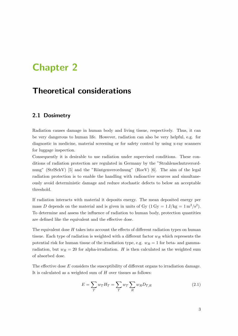
Figure 2.1 shows the connection between the protection quantities (left) and the measur-
able operative quantities (right).
Hp(3)
Hp(10)
Hp(0.07)
0.04
0.12
0.12
T
0.04
R
5-20
20
1
5
3
2
1
Figure 2.1: Protection quantities and their estimation over operative quantities.1: Weighting factors for different types of radiation. 2: Weighting factors for differenttissues in the human body. 3: Operative quantities. The values of the weighting factorsare defined in Ref. [7].
The operative quantities can be calculated via the measurable quantity Kerma (kinetic
energy released per unit mass). It is defined as the loss of kinetic energy from secondary
4
2.1 Dosimetry
particles per mass in a material. Secondary particles are produced if ionizing radiation
interacts with matter. For dosimetry applications the Kerma in air Ka is mainly used,
because the handling is very easy.In case of a secondary electron equilibrium the Kerma
is equal to the absorbed dose and therefore, it is the main quality of an irradiation field
and the other operative quantities can be easily calculated via conversion factors.
2.1.1 Personal dosimetry
According to StrlSchV [5] and RoeV [6], any person who can be occupationally exposed
to radiation has to be officially monitored. The official monitoring in Germany is con-
ducted by four individual dose monitoring services, the ”Strahlenmessstelle” of the Sen-
ate Department for the Environment, Transport and Climate Protection in Berlin, the
”Landesanstalt fur Personendosimetrie und Strahlenschutzausbildung” (LPS) in Berlin,
the individual monitoring service of the Materialprufungsamt North Rhine-Westphalia
(MPA NRW) in Dortmund and the ”Auswertestelle” (AWST) of the Helmholz Zentrum
Munich, ascending by number of monitored persons.
The dosemeters used for the official individual dosimetry have to fulfill national and
international standards [8, 9], e.g. the response of the dosemeter as a function of the
irradiation energy and angle has to be in a given range. Furthermore, all monitoring
services have to regularly participate in comparison measurements for quality assurance
of the European Radiation Dosimetry Group (EURADOS).
The individual monitoring service of the MPA NRW is the second largest measurement
facility with approximately 110 000 dosemeter evaluations per month. The main moni-
toring parameter in radiation protection dosimetry is Hp(10), which is currently done by
using film dosemeter which is described in the next section.
2.1.2 The film dosemeter
Film dosemeter consists of a photo-film and if the film gets irradiated it becomes darker.
The gray tone of the optical density of the film is directly correlated to the amount of
incoming irradiation.
The film itself is very sensitive to the irradiation energy as well as its angle. To achieve
the requirements to an official dosemeter, the gliding-shadow method was developed [10].
With a combination of two filters the energy and angular dependency of dosemeter re-
sponse can be reduced.
One filter consists of several metals and guarantees a good response for higher irradiation
energies, whereas the filter made of plastic provides a good response for lower energies.
5
Chapter 2 Theoretical considerations
For the analysis the two gray tones of the film under the two filters are examined and
differently weighted to induce an energy independent value so that the overall energy
dependency of the film can be compensated. The filters are placed at a certain distance
in front of the dosemeter and are designed so that the density of the film is independent
of the irradiation angle. Furthermore, the badge contains four lead pins to estimated the
direction of incident radiation by analyzing their shadow on the film. Two more filters
are added to distinguish between beta- and gamma-irradiation.
After the film is developed, it can be read out in a fully automated setup. The film
dosemeter does not loose signal due to thermal fading, which is explained in Section 2.3.
However, after its production, the film loses sensitivity due to accumulation of natural
radiation and is a single-use detector.
The film dosemeter is currently still the predominantly used dosemeter type in routine
dosimetry to monitor the whole body dose Hp(10). However, it loses its approval at the
end of 2024 and thus, the dosimetry services are in the process of switching to other types
of dosemeters, like thermoluminescence or optically stimulated luminescence. Thermo-
luminescence dosemeters are already used in various fields of dosimetry, e.g. beta-ring
dosemeter to measure the skin dose Hp(0.07).
2.2 Thermoluminescence
The phenomenon of thermoluminescence (TL) describes a process in which light is emit-
ted by an irradiated material when it is heated. The phenomenon is utilized in various
fields of radiation protection and dating.
This process can be divided into two steps, first the irradiation of the sample, second its
light emission during heating. The previous radioactive irradiation is essential to observe
the phenomenon, otherwise only black body radiation or incandescence, respectively, oc-
cur. Therefore, it is actually more accurate to call the phenomenon thermally stimulated
luminescence, because the heat is not the exclusive reason but rather the activator for
the photon emission, similar to optically stimulated luminescence (OSL) where an optical
laser stimulates the light output of an irradiated sample. However, the term TL is more
commonly used and thus, used in the following.
TL detectors are mainly made of material which are insulator, e.g. lithium fluoride or
calcium fluoride. The TL in these solids can be explained with the help of the band-model.
The uppermost band, which is completely filled with electron, is the valence band. The
electrons in this band are bound to the ions of the lattice. The conduction band is the
first band, which is generally empty.
If the sample is irradiated, electrons are exited from the valence band to the conduction
6
2.2 Thermoluminescence
band, where they are unbounded and can move freely before they return to their ground
state in the valence band.
However, there is no TL light emission during the return if the irradiated material is
pure and have no defects. To be able to undergo the effect of TL, a material needs
certain types of defects which are capable of trapping electrons and holes, coming from
the interaction of ionizing irradiation with material. Those defects can be inserted by
doping the material, e.g. LiF is often doped with magnesium and titanium (LiF:Mg,Ti)
to create traps. The energy levels of the traps lie between both bands, as shown in
Figure 2.2. The binding energy of a charge carrier to a trap is called trap depth.
1 2
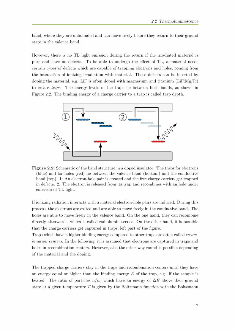
Figure 2.2: Schematic of the band structure in a doped insulator. The traps for electrons(blue) and for holes (red) lie between the valence band (bottom) and the conductiveband (top). 1: An electron-hole pair is created and the free charge carriers get trappedin defects. 2: The electron is released from its trap and recombines with an hole underemission of TL light.
If ionizing radiation interacts with a material electron-hole pairs are induced. During this
process, the electrons are exited and are able to move freely in the conductive band. The
holes are able to move freely in the valence band. On the one hand, they can recombine
directly afterwards, which is called radioluminescence. On the other hand, it is possible
that the charge carriers get captured in traps, left part of the figure.
Traps which have a higher binding energy compared to other traps are often called recom-
bination centers. In the following, it is assumed that electrons are captured in traps and
holes in recombination centers. However, also the other way round is possible depending
of the material and the doping.
The trapped charge carriers stay in the traps and recombination centers until they have
an energy equal or higher than the binding energy E of the trap, e.g. if the sample is
heated. The ratio of particles n/n0 which have an energy of ∆E above their ground
state at a given temperature T is given by the Boltzmann function with the Boltzmann
7
Chapter 2 Theoretical considerations
constant k.
n
n0= e−∆E/(kT ) (2.2)
For typical values of e.g. ∆E = 1.2 eV and T = 473 K the fraction n/n0 is smaller than
1 · 10−12. However, for such values TL light emission is observed and this is due to an
additional factor s, the so-called frequency factor. This factor was introduced in Ref. [2]
and describes the rate with which the electrons ”try” to escape. It is the product of the
frequency with which electron strikes the wall of the potential box of the trap and the
reflection coefficient on it. Thus, s also depend on the temperature of the sample, but
this dependency is very small and can be neglected in the following.
The probability, prelease, that an electron is released from a trap can be described as
prelease = se−∆E/(kT ). (2.3)
The value of s is in the range of (n/n0)−1 and thus, the electron is released from the
trap if its energy is equal to or higher than the binding energy. Consequently, the higher
the temperature the more electrons from deeper traps can be released. For application
of TL, the required energy is usually supplied by heating the sample.
During the heating, electrons are excited into the conduction band, from where they can
be either recombine with a hole in a recombination center under the emission of TL light
(see right part of Figure 2.2) or the electrons can be trapped again either in the same or
another trap, called re-trapping.
The simplified one trap one recombination center (OTOR) model is often used in litera-
ture to describe these processes, e.g. Ref. [2]. As the name of the model states, only one
kind of traps with a binding energy of ∆E = E and one kind of recombination center are
considered.
Ref. [2] assumes that in most cases the re-trapping can be neglected and presented Equa-
tion (2.4) which describes the intensity I of emitted TL light as a function of time t, where
n is the number electrons trapped with an energy of E at the time t and a temperature
T . The constant C includes all measurement efficiencies and is set to 1 in the following.
I(t) = −dn
dt= Cnse−E/(kT ) (2.4)
The model, in which re-trapping is neglected, is often referred to as first-order kinetics.
In this model the light emission is directly correlated to the excitation of electrons from
traps.
If the the amount of re-trapping is equal to that of recombination, the model is referred
to as second-order kinetics [11]. Everything in between is summarized in the model of
8
2.2 Thermoluminescence
general-order kinetics [12]. The difference between these models as well as an extension
to mixed-order kinetics are discussed in Refs. [13, 14, 15].
Equation (2.4) describes the TL intensity I in the OTOR model for one trap depth.
However, usually traps at different depths exist in a doped material and each trap depth
results in a separate glow peak. If the superposition of all glow peaks is plotted versus
the temperature T or versus the time t it is called glow curve.
Since the number of measured photons is proportional to the number of trapped elec-
trons, which is proportional to the incident irradiation dose, it is possible to use the TL
phenomenon for dosimetry. Thus, TL dosemeters are an alternative to the deprecated
film dosemeter presented in the previous section. Summaries of the State-of-the-art of
TL dosimetry applications can be found in Refs. [16, 17].
In addition to LiF:Mg,Ti, several other materials are suitable for TL dosimetry, e.g.
LiF:Mg,Cu,P, CaF2:Tm or CaSO4:Dy. Information about six commonly used TL ma-
terials and their characteristics can be found in Ref. [18] and references therein. The
dosemeters, investigated in the following, are produced with LiF:Mg,Ti. As the sensitive
TL material, MT-N is used, which is manufactured by Radcard [19].
LiF:Mg,Ti has five significant glow peaks, denoted by P1 to P5, in a temperature range
between room-temperature and 573 K, which is the readout temperature. The half-lifes
of the individual peaks depend of the depth of the trap and range from a few minutes to
several years, for more details on the different peaks see next section.
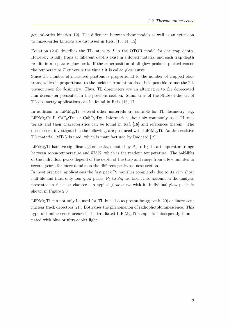
In most practical applications the first peak P1 vanishes completely due to its very short
half-life and thus, only four glow peaks, P2 to P5, are taken into account in the analysis
presented in the next chapters. A typical glow curve with its individual glow peaks is
shown in Figure 2.3
LiF:Mg,Ti can not only be used for TL but also as proton bragg peak [20] or fluorescent
nuclear track detectors [21]. Both uses the phenomenon of radiophotoluminescence. This
type of luminescence occurs if the irradiated LiF:Mg,Ti sample is subsequently illumi-
nated with blue or ultra-violet light.
9
Chapter 2 Theoretical considerations
350 400 450 500 550T in K
0
1000
2000
3000
4000
num
ber o
f pho
tons
in K
1
P2P3
P4P5
data
TL-DOS
Figure 2.3: Typical glow curve with a dose of Hp(10) = 15 mSv. The four individualglow peaks are plotted as dashed lines. The gray line which described the whole glowcurve is plotted to guide the eye.
2.3 Thermal fading in LiF:Mg,Ti
Trapped charge carriers can be released by applying energy in the form of heat as de-
scribed in the previous section. Due to Equation (2.3) there is a chance to release electrons
from their traps already at room-temperature. This phenomenon is called thermal fading
or simply fading.
Consequently, thermal fading results in a smaller TL signal when read out. For example
the signal of the used LiF:Mg,Ti dosemeters decreases by up to 30% in a typical routine
monitoring cycle of 40 d. The individual peaks are affected in different ways. High-
temperature peaks are more stable than low-temperature peaks, because shallow traps
can be released more easily by thermal stimulation than traps with higher activation
energies.
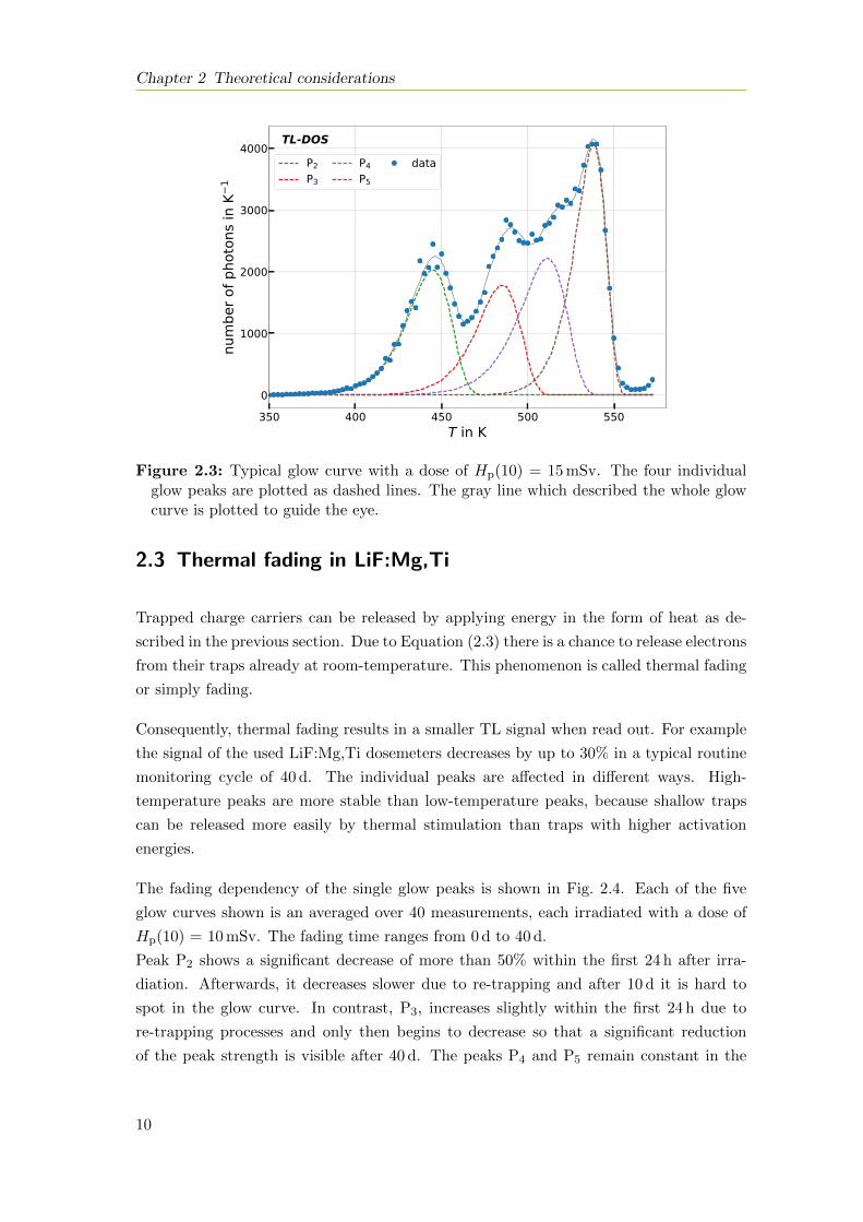
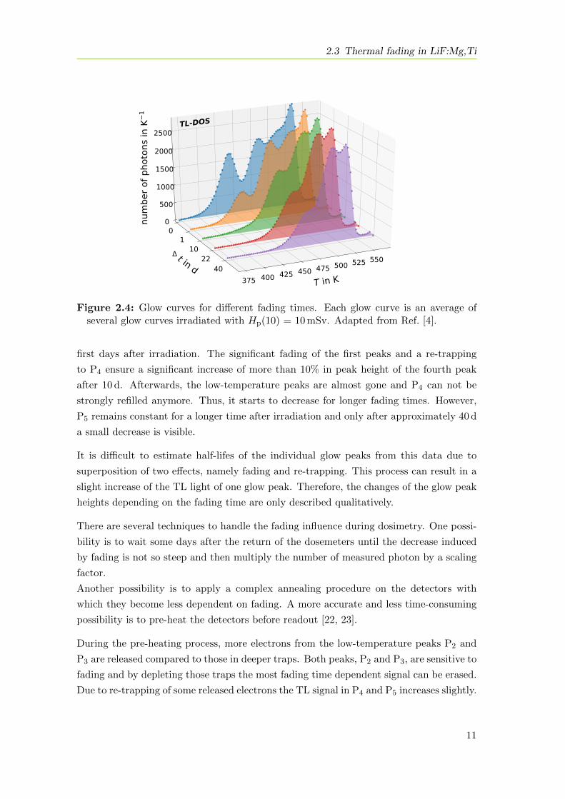
The fading dependency of the single glow peaks is shown in Fig. 2.4. Each of the five
glow curves shown is an averaged over 40 measurements, each irradiated with a dose of
Hp(10) = 10 mSv. The fading time ranges from 0 d to 40 d.
Peak P2 shows a significant decrease of more than 50% within the first 24 h after irra-
diation. Afterwards, it decreases slower due to re-trapping and after 10 d it is hard to
spot in the glow curve. In contrast, P3, increases slightly within the first 24 h due to
re-trapping processes and only then begins to decrease so that a significant reduction
of the peak strength is visible after 40 d. The peaks P4 and P5 remain constant in the
10
2.3 Thermal fading in LiF:Mg,Ti
T in K375 400 425 450 475 500 525 550t in d
01
1022
40
num
ber o
f pho
tons
in K
1
0
500
1000
1500
2000
2500TL-DOS
Figure 2.4: Glow curves for different fading times. Each glow curve is an average ofseveral glow curves irradiated with Hp(10) = 10 mSv. Adapted from Ref. [4].
first days after irradiation. The significant fading of the first peaks and a re-trapping
to P4 ensure a significant increase of more than 10% in peak height of the fourth peak
after 10 d. Afterwards, the low-temperature peaks are almost gone and P4 can not be
strongly refilled anymore. Thus, it starts to decrease for longer fading times. However,
P5 remains constant for a longer time after irradiation and only after approximately 40 d
a small decrease is visible.
It is difficult to estimate half-lifes of the individual glow peaks from this data due to
superposition of two effects, namely fading and re-trapping. This process can result in a
slight increase of the TL light of one glow peak. Therefore, the changes of the glow peak
heights depending on the fading time are only described qualitatively.
There are several techniques to handle the fading influence during dosimetry. One possi-
bility is to wait some days after the return of the dosemeters until the decrease induced
by fading is not so steep and then multiply the number of measured photon by a scaling
factor.
Another possibility is to apply a complex annealing procedure on the detectors with
which they become less dependent on fading. A more accurate and less time-consuming
possibility is to pre-heat the detectors before readout [22, 23].
During the pre-heating process, more electrons from the low-temperature peaks P2 and
P3 are released compared to those in deeper traps. Both peaks, P2 and P3, are sensitive to
fading and by depleting those traps the most fading time dependent signal can be erased.
Due to re-trapping of some released electrons the TL signal in P4 and P5 increases slightly.
11
Chapter 2 Theoretical considerations
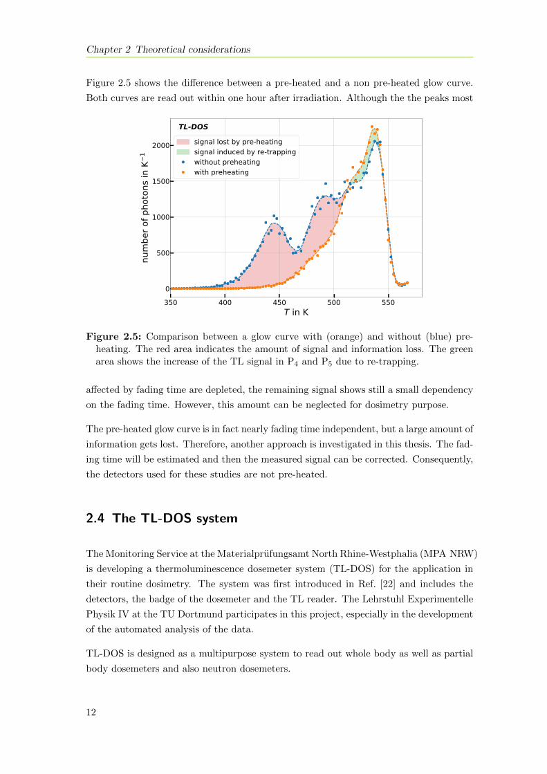
Figure 2.5 shows the difference between a pre-heated and a non pre-heated glow curve.
Both curves are read out within one hour after irradiation. Although the the peaks most
350 400 450 500 550T in K
0
500
1000
1500
2000nu
mbe
r of p
hoto
ns in
K1
signal lost by pre-heatingsignal induced by re-trappingwithout preheatingwith preheating
TL-DOS
Figure 2.5: Comparison between a glow curve with (orange) and without (blue) pre-heating. The red area indicates the amount of signal and information loss. The greenarea shows the increase of the TL signal in P4 and P5 due to re-trapping.
affected by fading time are depleted, the remaining signal shows still a small dependency
on the fading time. However, this amount can be neglected for dosimetry purpose.
The pre-heated glow curve is in fact nearly fading time independent, but a large amount of
information gets lost. Therefore, another approach is investigated in this thesis. The fad-
ing time will be estimated and then the measured signal can be corrected. Consequently,
the detectors used for these studies are not pre-heated.
2.4 The TL-DOS system
The Monitoring Service at the Materialprufungsamt North Rhine-Westphalia (MPA NRW)
is developing a thermoluminescence dosemeter system (TL-DOS) for the application in
their routine dosimetry. The system was first introduced in Ref. [22] and includes the
detectors, the badge of the dosemeter and the TL reader. The Lehrstuhl Experimentelle
Physik IV at the TU Dortmund participates in this project, especially in the development
of the automated analysis of the data.
TL-DOS is designed as a multipurpose system to read out whole body as well as partial
body dosemeters and also neutron dosemeters.
12
2.4 The TL-DOS system
However, the main focus is on the realization of a whole body TL dosemeter to simul-
taneously measure the personal dose equivalents Hp(10) and Hp(0.07) according to EN
62387 [9]. In addition, the dosemeters have to fulfill requirements of the Physikalisch-
Technische Bundesanstalt (PTB) [8], e.g. the response of the dosemeter as a function
of the irradiation energy and angle has to be in a given range. Furthermore Hp(10)
dosemeters must not measure more than 10% of the irradiation dose from a beta irradia-
tion. This so-called beta-criterion is required because beta irradiation is not expected to
contribute to the effective dose in a depth of 10 mm.
In comparison to a gliding shadow film dosemeter, the TL-DOS dosemeter has several
advantages. The sensitive material LiF:Mg,Ti, used for the detectors, is less energy
dependent and also tissue equivalent, which slightly simplifies the calibration process.
The detector of the TL-DOS dosemeter can be used multiple times because on the one
hand it is still sensitive to irradiation after readout and on the other hand it can be reset
to the initial state, a process known as annealing. This is done by heating the detector
to a temperature of 673 K so that all traps, which are responsible for the glow peaks up
to the readout temperature of 573 K, get depleted and the complete information on the
detector is erased before the detector is used again. Thus, the detector is not affected
by previous irradiations. This process ensures that the detector has the same sensitive
for every measurement. Furthermore the complete annealing offers the possibility to
calibrate every detector individually. After the readout and the annealing of the detector,
it is irradiated with a known dose and subsequent measured to estimate the calibration
factor.
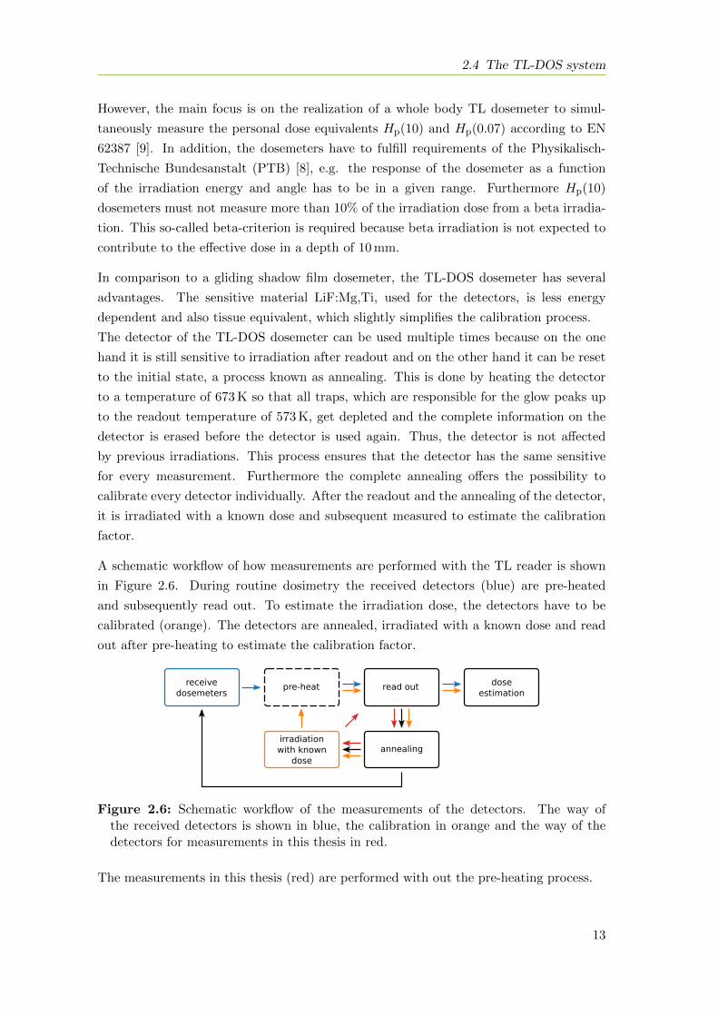
A schematic workflow of how measurements are performed with the TL reader is shown
in Figure 2.6. During routine dosimetry the received detectors (blue) are pre-heated
and subsequently read out. To estimate the irradiation dose, the detectors have to be
calibrated (orange). The detectors are annealed, irradiated with a known dose and read
out after pre-heating to estimate the calibration factor.
receivedosemeters
pre-heat read out dose estimation
irradiation with known
doseannealing
Figure 2.6: Schematic workflow of the measurements of the detectors. The way ofthe received detectors is shown in blue, the calibration in orange and the way of thedetectors for measurements in this thesis in red.
The measurements in this thesis (red) are performed with out the pre-heating process.
13
Chapter 2 Theoretical considerations
A disadvantage compared to the film dosemeter is that the LiF:Mg,Ti material shows
thermal fading, as described above. However, there are several techniques to overcome
the effect of fading, see Section 2.3. In addition this phenomenon can be used to estimate
the date of an irradiation, which is the main focus in this thesis. Furthermore, the glow
curve can be analyzed to get additional information to the irradiation dose.
2.4.1 Detectors
The detectors of the TL-DOS system are developed, produced and tested at the MPA NRW.
There are several detectors sizes for different dosemeters types, which are very similar in
composition.
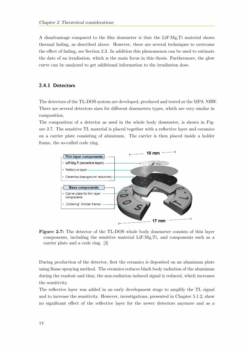
The composition of a detector as used in the whole body dosemeter, is shown in Fig-
ure 2.7. The sensitive TL material is placed together with a reflective layer and ceramics
on a carrier plate consisting of aluminum. The carrier is then placed inside a holder
frame, the so-called code ring.
Figure 2.7: The detector of the TL-DOS whole body dosemeter consists of thin layercomponents, including the sensitive material LiF:Mg,Ti, and components such as acarrier plate and a code ring. [3]
During production of the detector, first the ceramics is deposited on an aluminum plate
using flame spraying method. The ceramics reduces black body radiation of the aluminum
during the readout and thus, the non-radiation induced signal is reduced, which increases
the sensitivity.
The reflective layer was added in an early development stage to amplify the TL signal
and to increase the sensitivity. However, investigations, presented in Chapter 5.1.2, show
no significant effect of the reflective layer for the newer detectors anymore and as a
14
2.4 The TL-DOS system
consequence it is omitted. By omitting the additional step during the production process,
the production time of the detector can be reduced.
The sensitive TL material is MT-N. It is manufactured by Radcard [19] and has a natural
composition of 6LiF:Mg,Ti (∼5%) and 7LiF:Mg,Ti (∼95%). The LiF:Mg,Ti powder is
hot-sintered on the ceramics of the aluminum carrier plate. The amount of LiF:Mg,Ti
can be adjusted between 1 mg and 35 mg. For the standard detector of the TL-DOS
whole body dosemeter 15 mg are used, whereas the amount of LiF:Mg,Ti on a detector
for partial body dosemeters ranges from 1 mg to 5 mg to adjust the sensitivity of the
detector to the different required irradiation dose ranges.
The size of the aluminum carrier plate itself depends on the detector type as well. The
carrier plate of a standard detector is 10 mm in diameter and the smaller detectors, used
mainly for partial body dosemeters, have a diameter of 7 mm. On the bottom side of the
detector a data matrix, containing the detector identification number, is engraved with a
laser.
The aluminum code ring provides protection of the inner core and includes the detector
identification number in a human readable form. However, it is only used for the 10 mm
detectors. To read out the smaller 7 mm detectors with the same reader, an adapter
similar to the code ring is used.
More information about the detectors used for the studies in this thesis, can be found in
Chapter 5.1.
2.4.2 Dosemeter system
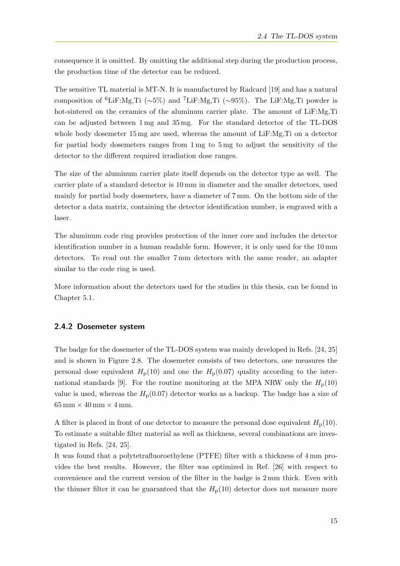
The badge for the dosemeter of the TL-DOS system was mainly developed in Refs. [24, 25]
and is shown in Figure 2.8. The dosemeter consists of two detectors, one measures the
personal dose equivalent Hp(10) and one the Hp(0.07) quality according to the inter-
national standards [9]. For the routine monitoring at the MPA NRW only the Hp(10)
value is used, whereas the Hp(0.07) detector works as a backup. The badge has a size of
65 mm× 40 mm× 4 mm.
A filter is placed in front of one detector to measure the personal dose equivalent Hp(10).
To estimate a suitable filter material as well as thickness, several combinations are inves-
tigated in Refs. [24, 25].
It was found that a polytetrafluoroethylene (PTFE) filter with a thickness of 4 mm pro-
vides the best results. However, the filter was optimized in Ref. [26] with respect to
convenience and the current version of the filter in the badge is 2 mm thick. Even with
the thinner filter it can be guaranteed that the Hp(10) detector does not measure more
15
Chapter 2 Theoretical considerations
Figure 2.8: Drawing of the dosemeter badge with two TL detectors, one measuresthe Hp(10) irradiation dose quality and one the Hp(0.07) quality. Left: Blister packcontaining the two detectors. Right: Enclosure with the PTFE filter (top) in front ofthe Hp(10) detector and a cone shaped gap (bottom) in front of the Hp(0.07) detector.[25]
than 10% of the irradiated dose from a beta irradiation and the beta-criteria is fulfilled.
In addition the filter flattens the dependency of dosemeter on the irradiation energy and
the irradiation.
In front of the other detector no additional filter is positioned and only the thin plastic
layer of the badge material provides filtering to measure the Hp(0.07) quality. A cone
shaped recess with an opening angle of 60° in front of the Hp(0.07) detector guarantees
a flat angle response for it as well.
In addition to the whole body dosemeter with two detectors, several other dosemeters are
investigated. A finger ring dosemeter to measure the partial skin dose Hp(0.07) using the
small detector elements was developed in Refs. [27, 28]. The smaller detectors were also
used to design an Hp(3) eye lens dosemeters and demonstrate its practicability [29]. Fur-
thermore, in Refs. [30, 31] first studies for the development of a neutron dosemeter based
on the TL-DOS system are performed. For this purpose detectors with pure 6LiF:Mg,Ti
and others with pure 7LiF:Mg,Ti are produced and combined in one dosemeter.
2.4.3 TL reader
The measurements presented in Chapter 4 are performed with the so-called Prototype II
TL reader [22]. It is designed for application in routine dosimetry and consists of different
16
2.4 The TL-DOS system
independent modules. Since these measurements, a new TL reader has been delivered.
It is design to be used in large-scale routine dosimetry and have a higher throughput
compared to the Prototype II. However, it is not used for measurements performed in
this thesis and thus, it is not introduced here, but details and first investigations on the
new reader can be found in Ref. [26].
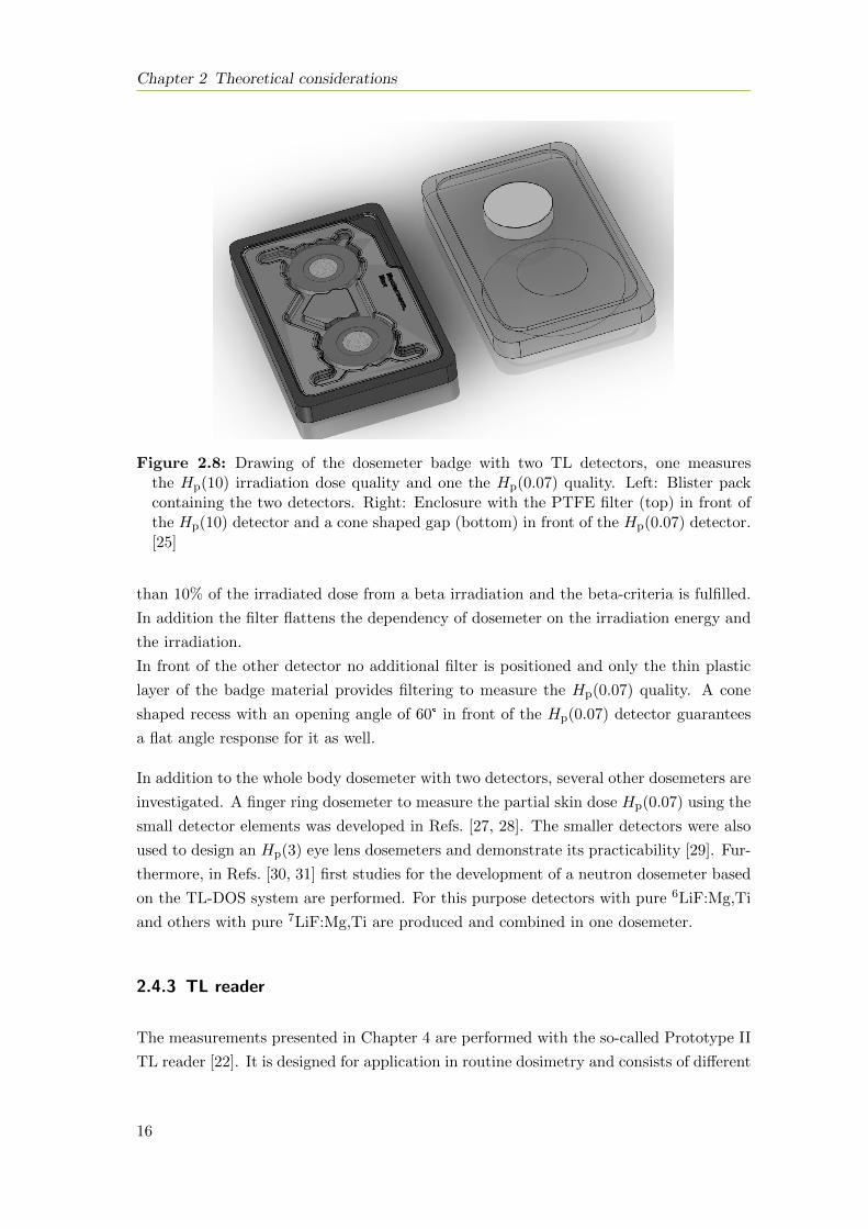
Figure 2.9 shows the Prototype II of the TL-DOS reader with its different modules (A-F)
for pre-heating, readout and annealing arranged in a circle around the transportation
unit.
Figure 2.9: Prototype II of the TL reader for the TL-DOS system. A: Holder for 32detectors, B: Scanner to read data matrix, C: Transportation unit, D: Pre-heatingstation, E: Measurement chamber with PMT, F: Annealing station.
Detectors can be placed in a holder wheel with 32 slots (A). The scanner (B), which
is mounted next to the holder, reads the data matrix with the detector identification
number to guarantee an accurate and fast identification of the placed detectors. The
transportation unit (C) is arranged in the middle to effectively handle the detectors
between the three heating stations and the holder wheel.
To overcome the effect of fading, the detectors can be pre-heated before the readout
[22, 23]. In the pre-heat station (D), the detectors are placed on a constant-temperature
cartridge and are heated up for 10 s to 428 K. Afterwards, they are cooled down to room-
temperature for 3 s and read out subsequently. Since the fading time is analyzed in this
thesis and pre-heating erases nearly all information about it, the pre-heating device is not
17
Chapter 2 Theoretical considerations
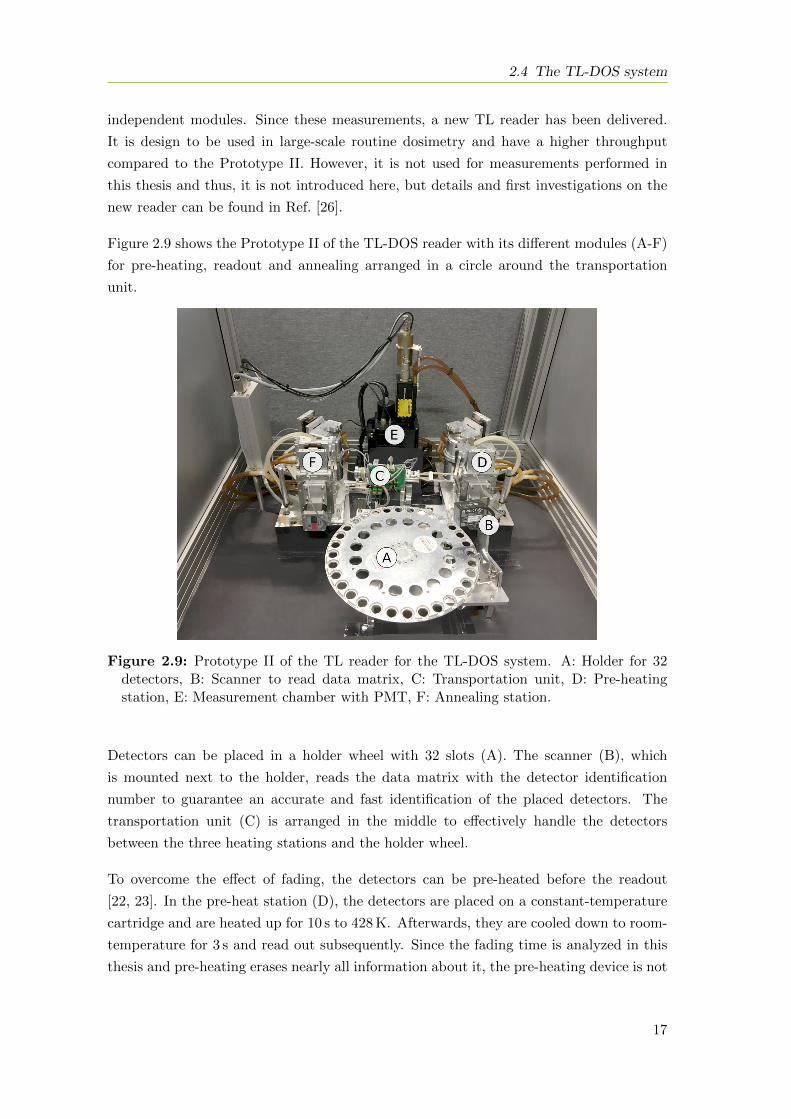
Figure 2.10: Readout unit withmeasurement chamber consistingof a constant-temperature car-tridge and a PMT. Adapted fromRef. [22].
used here. However, it is very important for routine dosimetry because it allows a much
easier calibration. If the detectors are pre-heated, the calibration measurements can be
read out directly after their irradiation. Otherwise they would have to be stored until
they show a similar fading as the monitoring measurements from the received detectors.
The key component of the reader is the readout unit (E) which is also shown in Fig-
ure 2.10. The measurement chamber consists of a constant-temperature cartridge and a
photo multiplier tube (PMT). The heating plate has a constant temperature of 573 K
and the resulting exponential heating of the detector allows to obtain a glow curve in
about 10 s. For application in routine dosimetry, the TL signal is recorded for 12 s to 15 s.
The PMT has a sampling frequency of 10 ms and is able to count single photon and
simultaneously measure the photo current. The single photon mode yields accurate glow
curves for low irradiation dose, which are typical for routine dosimetry. For irradiation
doses higher than approximately 100 mSv the single photon mode is not reliable due to
an overflow of photons and the information from the photon current mode has to be used
for analysis. The exact threshold is investigated in Ref. [32].
During the development of the reader, the main focus was on reaching high sensitivity
to low irradiation doses. Therefore, the PMT is placed very closed to the detector which
leaves no space to include a sensor to measure the temperature of the detector during
heating.
The sensitivity is also increased by reducing the non-radiation induced signal. This back-
ground stems from three different sources, namely thermal radiation, radiation related to
chemiluminescence effects and the instrumental background [33].
The instrumental background is e.g. induced by the dark current of the PMT. It is
18
2.4 The TL-DOS system
minimized by cooling the PMT and optimizing the threshold of PMT which was done
by manufacturer of the reader. The thermal radiation is emitted by the detector dur-
ing heating and the heating plate itself. Using appropriate optical filters can reduce the
amount of black body radiation detected by the PMT.
The signal related to chemiluminescence effects can be suppressed by flushing the mea-
surement chamber with nitrogen. With these arrangements the non-radiation induced
signal can be significantly reduced but not completely canceled and thus, it is considered
in the glow curve deconvolution (GCD) of the glow curve as described in Chapter 3.
The annealing station (F) is identical in construction to the pre-heat station. However,
the heating element for annealing of the detectors has a constant temperature of 673 K.
The detector is heated up to this temperature for 15 s and is then cooled down to room-
temperature in another 15 s. The high temperature gradient results in a high sensitivity
of the LiF:Mg,Ti material [34]. During this process all traps get depleted and the detector
is reset to its initial state and thus, it can be reused for dosimetry purpose.
The TL reader is designed to reach a very low detection limit and to have a high through-
put. All stations for pre-heating, readout and annealing are in one device and no time-
consuming transportation between different devices has to be realized. In addition, all
heating stations use constant-temperature cartridges resulting in a fast exponential heat-
ing of the detectors and thus, the reader has a high throughput. The lower detection
limit of 100 µSv, requested by the PTB [8], can easily be reached as calculations show in
Ref. [35].
2.4.4 Evaluation and analysis software
For the analysis presented in this thesis, multiple custom-made software packages are
written in Python using several open-source packages. Most algorithms and calculations
in the temperature reconstruction and GCD, described in Chapter 3, including the fitting
procedures are implemented by using functions from the SciPy library [36].
With the custom-made software package, glow curves are automatically imported, the
temperature is reconstruction and a GCD is performed. The results are saved in DataFrames
of the pandas library [37], which can be exported to many different types of output files.
This software package allows to perform a complete analysis including calibration and
irradiation dose estimation. Furthermore, all corrections presented in Chapter 5 are in-
cluded as well and can be applied during an analysis.
The machine learning which is presented in Chapter 7 is also included in the software
package and uses the scikit-learn library [38]. For visualization and plotting the open-
source packages Matplotlib [39] and Seaborn [40] are used.
19

20
Chapter 3
Glow curve modeling and fitting
A thermoluminescence (TL) glow curve typically consists of several glow peaks. Ref. [2]
introduced the first-oder kinetics model of Equation (2.4) which describes the TL inten-
sity I of a single glow peak, as presented above. By assuming a linear heating profile,
T (t) = T0 + βt, and integrating the TL intensity with respect to the temperature T ,
Equation (2.4) becomes
I(T ) = s · n0 · e−EkT · exp
(− sβ
∫ T
T0
e−E
kT ′ dT ′). (3.1)
E represents the activation energy of the glow peak, s is the so-called frequency factor,
n0 is the initial concentration of trapped charge carriers and k is the Boltzmann constant.
The heating of the TL material from an initial temperature T0 is described by the heating
rate β.
3.1 Transformation from time to temperature scale
The emitted TL intensity of the heated sample depends on the temperature T , as de-
scribed in Equation (3.1). Due to sensitivity issues, the current TL-DOS reader does not
allow to measure the temperature T and instead the glow curve is recorded as a function
of time t during the readout. Thus, a transformation from time to temperature scale is
used to offer the possibility of a glow curve deconvolution (GCD). Since this technique
was describe in Ref. [3, 4], some improvements have been made.
To read out the detectors, they are placed on a constant-temperature cartridge with a
heating temperature Theat of 573 K, as described in Chapter 2.4.3. This results in an
exponential heating of the detector T (t), see e.g. Ref. [41],
T (t) = Theat − (Theat − Tstart) · e−αt, (3.2)
21
Chapter 3 Glow curve modeling and fitting
where Tstart is the temperature of the detector at the beginning of the measurement and
α is the exponential heating parameter which depends on the heat transfer between the
heating cartridge and the detector.
The model shown in Equation (3.2) does not consider additional effects like radiative
cooling or the temporary temperature decrease of the heating plates directly at the be-
ginning of the measurement due to the placing of a cold detector on the contact heating
supply.
The influences of several cooling effects are investigated for example in Refs. [42, 43]. Both
developed a generalized model by adding additional terms of cooling and heat transfer
inside the detector to describe the real heating as accurately as possible. The information
about the exact heating profile is either used to fine-tune the gas temperature of their
reader or to adjust the set heating profile.
However, the heating profile is only used to convert the glow curves from time to tempera-
ture domain, thus the basic detector temperature model is sufficient. A more sophisticated
heating function with additional parameters would even result in an under-estimated fit-
procedure, which is described below.
Due to slightly different heat transfer between heating plate, detector and the sensitive
material, the exact temperature profile differs for each readout. These differences arise
from fabrication tolerances and the usage of contact heating, resulting in glow curves
with variable length in the time domain, see the left part of Figure 3.2. Therefore, it is
not possible to use one global function to transform the glow curves from the time to the
temperature domain. Instead, a transformation is calculated for every single glow curve,
based on their individual heating function, as describe in the following.
The reconstruction can be done with the custom-made software package introduced in
Chapter 2.4.4. First, the region of the total recorded glow curve, where the glow peaks
arise, is estimated, the so-called region of interest (RoI). In dosimetry this region is
sometimes called region of dosimetric interest. The glow curve is highly smoothed with a
Savitzky-Golay filter [44] so that the single glow peaks are combined in one broad peak.
From the maximum of this one peak the boarders of the RoI are estimated by searching
for a given threshold on the TL intensity.
For the transformation from time to temperature domain, the number of individual glow
peaks have to be known. If the number is known, e.g. due to known fading time, it can
be used directly for the estimation of the peak positions. Otherwise, the number of peaks
have to be estimated. This can be done by calculating the second derivative of the glow
curve using the Savitzky-Golay filter and count the number of zero-crossings or rather
the number of inflection points to determine the number of peaks.This method works quit
well for typical glow curves. However, it is difficult to estimate the number of peaks for
22
3.1 Transformation from time to temperature scale
glow curves shorter than 6 s via the second derivative because the single peaks can not
be distinguished anymore. This could be circumvented if a PMT with a higher sampling
rate would be used.
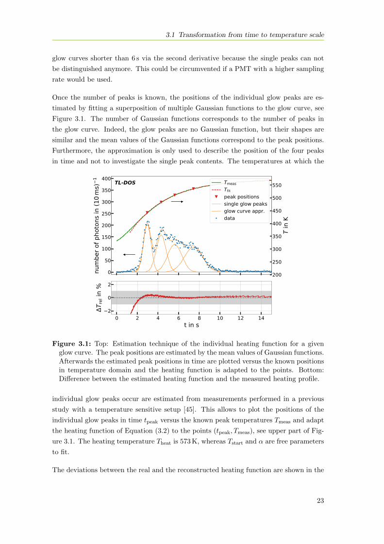
Once the number of peaks is known, the positions of the individual glow peaks are es-
timated by fitting a superposition of multiple Gaussian functions to the glow curve, see
Figure 3.1. The number of Gaussian functions corresponds to the number of peaks in
the glow curve. Indeed, the glow peaks are no Gaussian function, but their shapes are
similar and the mean values of the Gaussian functions correspond to the peak positions.
Furthermore, the approximation is only used to describe the position of the four peaks
in time and not to investigate the single peak contents. The temperatures at which the
0
50
100
150
200
250
300
350
400
num
ber o
f pho
tons
in (1
0ms)
1
200
250
300
350
400
450
500
550
T in
K
TmeasTfitpeak positionssingle glow peaksglow curve appr.data
0 2 4 6 8 10 12 14t in s
2
0
2
T rel
in %
TL-DOS
Figure 3.1: Top: Estimation technique of the individual heating function for a givenglow curve. The peak positions are estimated by the mean values of Gaussian functions.Afterwards the estimated peak positions in time are plotted versus the known positionsin temperature domain and the heating function is adapted to the points. Bottom:Difference between the estimated heating function and the measured heating profile.
individual glow peaks occur are estimated from measurements performed in a previous
study with a temperature sensitive setup [45]. This allows to plot the positions of the
individual glow peaks in time tpeak versus the known peak temperatures Tmeas and adapt
the heating function of Equation (3.2) to the points (tpeak, Tmeas), see upper part of Fig-
ure 3.1. The heating temperature Theat is 573 K, whereas Tstart and α are free parameters
to fit.
The deviations between the real and the reconstructed heating function are shown in the
23
Chapter 3 Glow curve modeling and fitting
bottom part of Figure 3.1. Due to the aforementioned initial decrease of the temperature
of the heating plate due to the cold detector which is not described by the ideal heating
profile of Equation (3.2), it may happen that Tstart is lower than actual room-temperature.
However, this apparent deviation between the real and the reconstructed heating function
only occurs at the beginning of heating before the start of the RoI.
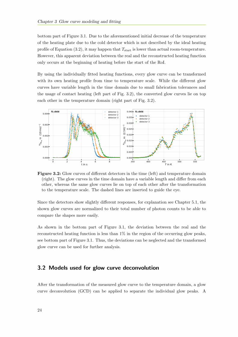
By using the individually fitted heating functions, every glow curve can be transformed
with its own heating profile from time to temperature scale. While the different glow
curves have variable length in the time domain due to small fabrication tolerances and
the usage of contact heating (left part of Fig. 3.2), the converted glow curves lie on top
each other in the temperature domain (right part of Fig. 3.2).
0 2 4 6 8t in s
0.000
0.001
0.002
0.003
0.004
N/ N
sig in
(10
ms)
1
detector 1detector 2detector 3
TL-DOS
350 400 450 500 550T in K
0.000
0.005
0.010
0.015
0.020
0.025
0.030
0.035
0.040
N/ N
sig in
(2.
5K)
1
detector 1detector 2detector 3
TL-DOS
Figure 3.2: Glow curves of different detectors in the time (left) and temperature domain(right). The glow curves in the time domain have a variable length and differ from eachother, whereas the same glow curves lie on top of each other after the transformationto the temperature scale. The dashed lines are inserted to guide the eye.
Since the detectors show slightly different responses, for explanation see Chapter 5.1, the
shown glow curves are normalized to their total number of photon counts to be able to
compare the shapes more easily.
As shown in the bottom part of Figure 3.1, the deviation between the real and the
reconstructed heating function is less than 1% in the region of the occurring glow peaks,
see bottom part of Figure 3.1. Thus, the deviations can be neglected and the transformed
glow curve can be used for further analysis.
3.2 Models used for glow curve deconvolution
After the transformation of the measured glow curve to the temperature domain, a glow
curve deconvolution (GCD) can be applied to separate the individual glow peaks. A
24
3.2 Models used for glow curve deconvolution
superposition of four peaks and a theoretically motivated empirical background function
is adapted to the glow curve to obtain information about the individual peaks.
3.2.1 Glow curve model
The glow curve model of Equation (3.1) contains an exponential integral∫ TT0
e−E
kT ′ dT ′
that has no analytic solution (see e.g. Ref. [46]).
To calculate the TL intensity, the exponential integral can be computed numerically.
However, a numerical integration is time consuming, especially during a minimization
procedure. Therefore, different approximations were developed and described over time.
An intercomparison of different models in Refs. [47, 48] reveals partly large deviations
between Equation (3.1) and some of theses approximations, resulting in an ineffective
GCD. An alternative to these not so suitable approximations is presented in Ref. [46],
which describes the glow curve very well and provides a reliable GCD.
Furthermore, it was also tried to use well-established statistic functions like the Weibull
distribution or the Logistic asymmetric distribution to describe a single TL glow peak [49,
50]. However, both distributions have an additional parameter with respect to the other
functions and are thus more difficult to minimize during the GCD fit.
In contrast to the linear heating assumed in Equation (3.1), the current TL-DOS reader
has a constant-temperature cartridge resulting in an exponential heating of the detectors.
The heating rate β of an exponential heating profile can be described as
β =dT
dt= α(Theat − T ), (3.3)
where α is the exponential heating factor and Theat the constant temperature of the
heating plates. With Equation (3.3), the Equation (3.1) can be transformed to
I(T ) = s · n0 · e−EkT · exp
(− sα
∫ T
T0
e−E
kT ′
Theat − T ′dT ′
). (3.4)
By using the approximation presented in Refs. [51, 52], the TL intensity I in Equa-
tion (3.4) can be transformed from I(T, n0, s, E) to I(T, Im, Tm, E) to guarantee an effec-
tive GCD. The parameter Im describes the intensity of glow peak maximum and Tm its
position in the temperature domain, comparable to the same parameters in Ref. [46].
The shape of a glow peak is described by three parameters Im, Tm and E, which has the
advantage that it is possible to directly estimate Im and Tm experimentally for a single
glow peak before the actual GCD fit. However, it should be noted that E now represents
an effective trap depth and no longer the actual activation energy of the glow peak.
25
Chapter 3 Glow curve modeling and fitting
In Refs. [51, 52] the exponential integral in Equation (3.4) is approximated by asymp-
totic series as well as convergent series. A comparison between the numerical integral of
Equation (3.4) and the integral of the approximation in Refs. [51, 52] shows a deviation
less than 0.001%.
Both, Equation (3.1) and Equation (3.4) describe the TL intensity I(T ) of one single glow
peak as a function of temperature. However, the glow curves of common TL materials
e.g. LiF:Mg,Ti contain multiple glow peaks, see Chapter 2.2 and thus, a superposition of
four times Equation (3.4) is used to describe the TL intensity of a complete glow curve.
3.2.2 Background model
In addition to the different glow peaks, the measured glow curve contains non-radiation
induced signal. This background stems from three different sources which can be divided
into a temperature independent and a temperature dependent part, see e.g. Ref. [42, 33].
The instrumental background is temperature independent and is mostly induced by the
dark current of the PMT. The thermal radiation can be divided in a temperature in-
dependent part which is caused by the constant-temperature heating element and the
warm walls of the measurement chamber and a temperature dependent fraction which is
emitted by the detector during heating. The third part of the background contribution
is the temperature dependent radiation related to chemiluminescence effects.
During the conceptual design of the reader, different arrangements, which are explained in
Chapter 2.4.3, were made to reduce the background effects. However, the non-radiation
induced signal can not be completely canceled and thus, it has to be considered in a
GCD.
The background can be approximated by a constant plus an exponential term, Ibg; lit,
as e.g. in Refs. [53, 54] for a readout with linear heating or e.g. in Ref. [55] for a read-
out with an exponential heating. The constant describes the temperature independent
part of the background and the exponential term combines all temperature dependent
contributions.
Compared to the references, a linear term is added to improve the agreement with the
measured background. These empirical investigations lead to a background model of
Ibg; lin = a+ b · T + c · ed·T , (3.5)
where a, b, c and d are free fit parameters and T the temperature of the detector during
readout. Equation (3.5) describes background for most parts of the glow curve very well
and thus, it is used for the analysis presented in Section 6 to model the background of
26
3.2 Models used for glow curve deconvolution
the TL-DOS system.
However, a small deviation between the measured glow curve and the fitted function is
visible at higher temperatures after the glow peak P5, at about 560 K. Since the deviation
is similar for every glow curve, the influence of the difference at higher temperatures is
marginal as long as the GCD is used for peak separation to get information about the
single peak contents and no evaluation of kinetic parameters is done.
Equation (3.5) is optimized to improve the consistency between the measured glow curve
and the fitted function at higher temperatures as well. The glow curve is recorded as a
function of time and thus, the temperature independent part of the background, like the
noise of the PMT during readout, is constant in the recorded glow curve. This constant
term is transformed to ∝ 1/T during the conversion from time to temperature scale.
The temperature, and thus time, dependent part of the background is related to the
Planck equation which describes the spectral radiance of a body as a function of the
temperature T and the wavelength λ
Bλ(λ, T ) =2hc2
λ5
1
ehc/(λkBT ) − 1, (3.6)
where k is the Boltzmann constant, h is the Planck constant, and c is the speed of light
in the medium. The equation to describe the black body radiation is integrated over all
occurring wavelengths resulting in a term ∝ T 3 · e1/T , see Ref. [42]. Since the emitted
intensity is binned in temperature, empirical investigations show that the temperature
dependent part of the background can be approximated by an exponential function ∝eT [56] as shown in Figure 3.3.
The function to describe the non-radiation induced signal, Ibg, is a superposition of the
temperature independent and the temperature dependent part of the background and
can be parameterized as
Ibg; reci =a
b− T+ c · ed·T , (3.7)
where a, b, c and d are free fit parameters and T the temperature of the detector during
readout.
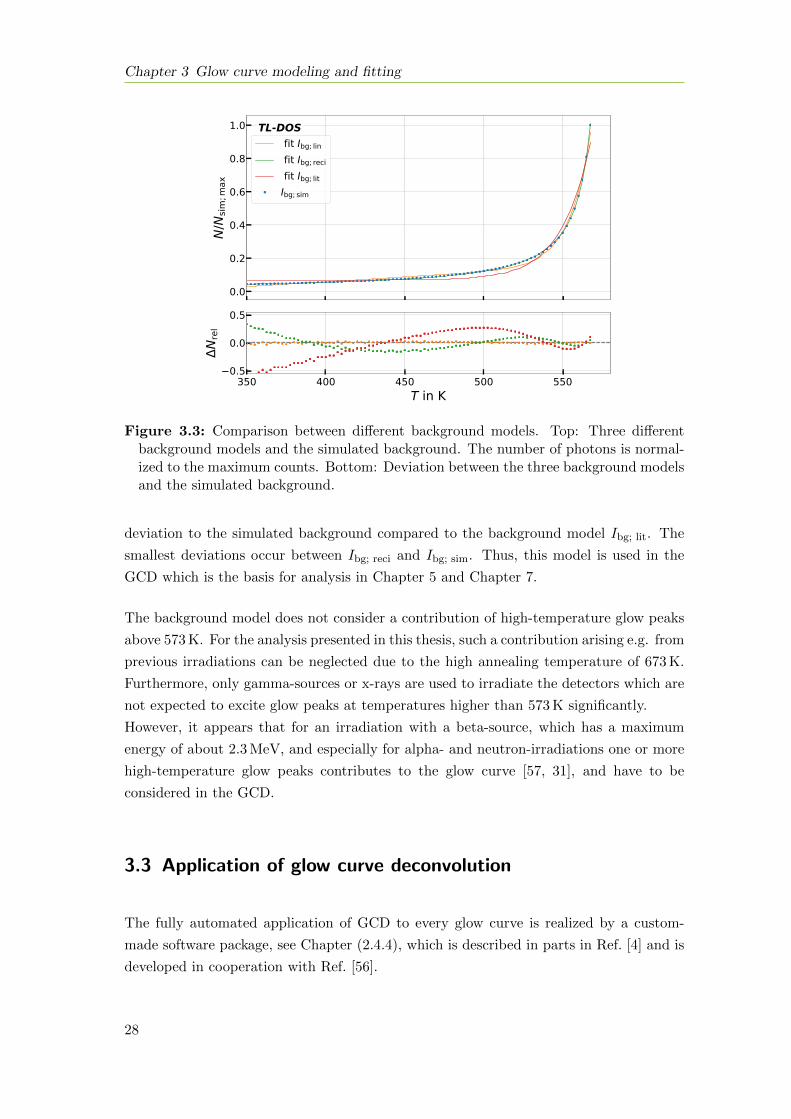
Figure 3.3 shows the comparison between the different background models as well as
the deviation of those to a simulated background, Ibg; sim. The number of photons are
normalized to the maximum value of the simulated data, because the shapes of the
different models are compared.
To estimate the simulated background the Planck equation is integrated with respect to
the wavelength sensitivity of the reader and a constant background, which is transformed
from time to temperature domain, is added. It is clearly visible that Ibg; lin shows smaller
27
Chapter 3 Glow curve modeling and fitting
0.0
0.2
0.4
0.6
0.8
1.0
N/N
sim;m
ax
fit Ibg; lin fit Ibg; reci fit Ibg; litIbg; sim
350 400 450 500 550T in K
0.5
0.0
0.5
Nre
l
TL-DOS
Figure 3.3: Comparison between different background models. Top: Three differentbackground models and the simulated background. The number of photons is normal-ized to the maximum counts. Bottom: Deviation between the three background modelsand the simulated background.
deviation to the simulated background compared to the background model Ibg; lit. The
smallest deviations occur between Ibg; reci and Ibg; sim. Thus, this model is used in the
GCD which is the basis for analysis in Chapter 5 and Chapter 7.
The background model does not consider a contribution of high-temperature glow peaks
above 573 K. For the analysis presented in this thesis, such a contribution arising e.g. from
previous irradiations can be neglected due to the high annealing temperature of 673 K.
Furthermore, only gamma-sources or x-rays are used to irradiate the detectors which are
not expected to excite glow peaks at temperatures higher than 573 K significantly.
However, it appears that for an irradiation with a beta-source, which has a maximum
energy of about 2.3 MeV, and especially for alpha- and neutron-irradiations one or more
high-temperature glow peaks contributes to the glow curve [57, 31], and have to be
considered in the GCD.
3.3 Application of glow curve deconvolution
The fully automated application of GCD to every glow curve is realized by a custom-
made software package, see Chapter (2.4.4), which is described in parts in Ref. [4] and is
developed in cooperation with Ref. [56].
28
3.3 Application of glow curve deconvolution
To separate the single glow peaks, the recorded glow curve is transformed to the temper-
ature domain first by using three or four peaks depending on the glow curve as described
in Section 3.1.
Afterwards a superposition of four glow peaks, described by the approximation of Equa-
tion (3.4) and the background model, described by Equation (3.7) is adapted to the glow
curve. The fit function consists of 16 parameters, three for each of the four glow peaks
and four additional ones to describe the background.
In many publications Im and Tm are estimated before the actual fitting procedure. If
the glow curve consists of only a single glow peak the estimation of the peak height and
position is easily possible. However, for a multi-peak glow curve with overlapping glow
peaks such an estimation does not provide reliable results and thus, those are left free to
vary in the fit procedure.
To stabilize the fit with 16 free parameters, a pre-fit is performed using the simplified
model of Ref. [46] to estimate start-values for Im, Tm and E. This approximation as-
sumes a linear heating profile, but it is a fast and very effective possibility to estimate
approximate start-values for the GCD. The pre-fit itself uses the previously measured
peak temperatures as initial values.
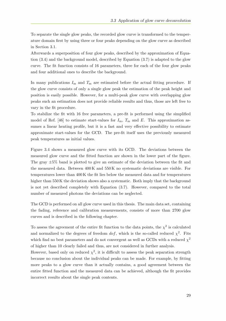
Figure 3.4 shows a measured glow curve with its GCD. The deviations between the
measured glow curve and the fitted function are shown in the lower part of the figure.
The gray ±5% band is plotted to give an estimate of the deviation between the fit and
the measured data. Between 400 K and 550 K no systematic deviations are visible. For
temperatures lower than 400 K the fit lies below the measured data and for temperatures
higher than 550 K the deviation shows also a systematic. Both imply that the background
is not yet described completely with Equation (3.7). However, compared to the total
number of measured photons the deviations can be neglected.
The GCD is performed on all glow curve used in this thesis. The main data set, containing
the fading, reference and calibration measurements, consists of more than 2700 glow
curves and is described in the following chapter.
To assess the agreement of the entire fit function to the data points, the χ2 is calculated
and normalized to the degrees of freedom dof , which is the so-called reduced χ2. Fits
which find no best parameters and do not convergent as well as GCDs with a reduced χ2
of higher than 10 clearly failed and thus, are not considered in further analysis.
However, based only on reduced χ2, it is difficult to assess the peak separation strength
because no conclusion about the individual peaks can be made. For example, by fitting
more peaks to a glow curve than it actually contains, a good agreement between the
entire fitted function and the measured data can be achieved, although the fit provides
incorrect results about the single peak contents.
29
Chapter 3 Glow curve modeling and fitting
0
1000
2000
3000
4000
num
ber o
f pho
tons
in K
1 single glow peaksglow curve fitdata
350 400 450 500 550T in K
200
0
200
N
±5%
TL-DOS
Figure 3.4: Measured glow curve (blue) with the separation in the individual glow peaks(orange). The deviations between the measured data and the GCD are shown at thebottom. The gray ±5% band is plotted to guide the eye and give an estimate of thedeviation between the fit and the measured data.
To nevertheless identify failed peak separations, an inter quartile range (IQR) outlier
detection is used. It is assumed that the majority of the fits provides a correct peak
separation and that only a few peak separations fail. The IQR is the distance between
the 25th percentile, Q1, and the 75th percentile, Q3. It is assumed that the parameters
resulting from the GCD are normally distributed and show no skewness for the same
irradiation and readout scenario.
In an IQR outlier detection, usually values which are lower than Q1− 1.5·IQR and those
which are higher than Q3 + 1.5·IQR are determined as outliers. For the studies in this
thesis, an outlier criterion of ±3·IQR is used to only identify extreme outliers. Only the
results from reliable peak separation are used for further investigations.
Overall it is noted that the GCD provides reliable results for glow curves which are longer
than 5 s. For shorter glow curves a peak separation is challenging and more fits fail or
provide no reliable results.
30
Chapter 4
Measurements and data sets
The majority of investigations presented in this thesis are based on the same data sets as
described in Ref. [4]. For the fading studies and the calibration measurements 800 newly
produced detectors are used. Furthermore, a set of 22 detectors is provided as a reference
sample, as recommended in Ref. [58]. These reference detectors have already been uses
many times and have a well known response.
To study the influence of fading time detectors are irradiated and then stored for differ-
ent lengths of time. The measurements are all performed with the TL reader which is
described in Chapter 2.4.3.
Before the irradiation all detectors are annealed to reset them to the same initial state.
Within a maximal time of 2 h after their annealing, the detectors are irradiated once using
a 137Cs source. Unless otherwise noted, the irradiation doses correspond to Hp(10) doses.
After the irradiation the detectors are stored in an isolated box to guarantee constant
environmental conditions particularly with regard to temperature and humidity. The box
is also lightproof to avoid influences like optical annealing or stimulation.
The annealing and irradiation of the detectors were planned in such a way that all de-
tectors could be read out within about two weeks to guarantee similar conditions during
read out. After the detector is placed on the heating plate, the TL signal is recorded
for 20 s. This measurement duration was chosen to include both the whole glow curve
with about 10 s and the background for additional 10 s and thus, a robust GCD can be
performed afterwards.
For the fading studies a total of 1600 measurements were performed. The detectors were
divided into groups of 40. For every fading time four sets of detectors were irradiated, each
with one of four different doses, see Table 4.1. Every time directly before an irradiation
the corresponding detectors were annealed.
For calibration of the irradiation 450 measurements were performed. The detectors were
grouped in batches of 50 and were irradiated with nine different irradiation doses ranging
31
Chapter 4 Measurements and data sets
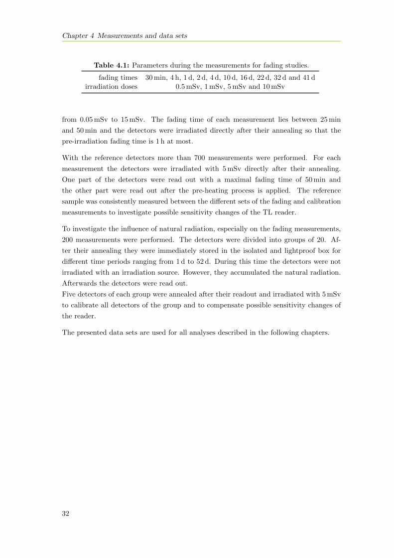
Table 4.1: Parameters during the measurements for fading studies.
fading times 30 min, 4 h, 1 d, 2 d, 4 d, 10 d, 16 d, 22 d, 32 d and 41 dirradiation doses 0.5 mSv, 1 mSv, 5 mSv and 10 mSv
from 0.05 mSv to 15 mSv. The fading time of each measurement lies between 25 min
and 50 min and the detectors were irradiated directly after their annealing so that the
pre-irradiation fading time is 1 h at most.
With the reference detectors more than 700 measurements were performed. For each
measurement the detectors were irradiated with 5 mSv directly after their annealing.
One part of the detectors were read out with a maximal fading time of 50 min and
the other part were read out after the pre-heating process is applied. The reference
sample was consistently measured between the different sets of the fading and calibration
measurements to investigate possible sensitivity changes of the TL reader.
To investigate the influence of natural radiation, especially on the fading measurements,
200 measurements were performed. The detectors were divided into groups of 20. Af-
ter their annealing they were immediately stored in the isolated and lightproof box for
different time periods ranging from 1 d to 52 d. During this time the detectors were not
irradiated with an irradiation source. However, they accumulated the natural radiation.
Afterwards the detectors were read out.
Five detectors of each group were annealed after their readout and irradiated with 5 mSv
to calibrate all detectors of the group and to compensate possible sensitivity changes of
the reader.
The presented data sets are used for all analyses described in the following chapters.
32
Chapter 5
Preparatory study
The measurements, described in the previous chapter, are used to investigate detector
properties, sensitivity changes of the whole readout system and environmental influences
on the measurements. These preparatory studies are performed in order to estimate
their impact on the fading and calibration measurements and to develop appropriate
corrections.
Investigations concerning the detector response include the impact of different amounts
of LiF:Mg,Ti as well as the impact of a reflective layer on the detectors. In addition, the
individual response of different detector series is compared. The reference measurements
are used to estimate sensitivity changes of the readout system. Furthermore, the impact
of natural radiation on the fading measurements is studied.
5.1 Impact of production methods on the detector response
During the development of the production process for the TL detectors, different pro-
duction methods have been adapted to simplify the production process and physically
motivated changes are made to improve the detectors.
With the data taken for this thesis (see Chapter 4), it is possible for the first time to
study the impact of those changes based on high statistics and to review the previous
results.
5.1.1 Amount of LiF
During the production process a small amount of LiF:Mg,Ti powder is deposited on the
pretreated aluminum carrier plate, see Chapter 2.4. The exact quantity deviates slightly
between the different detector series and the individual detectors.
33
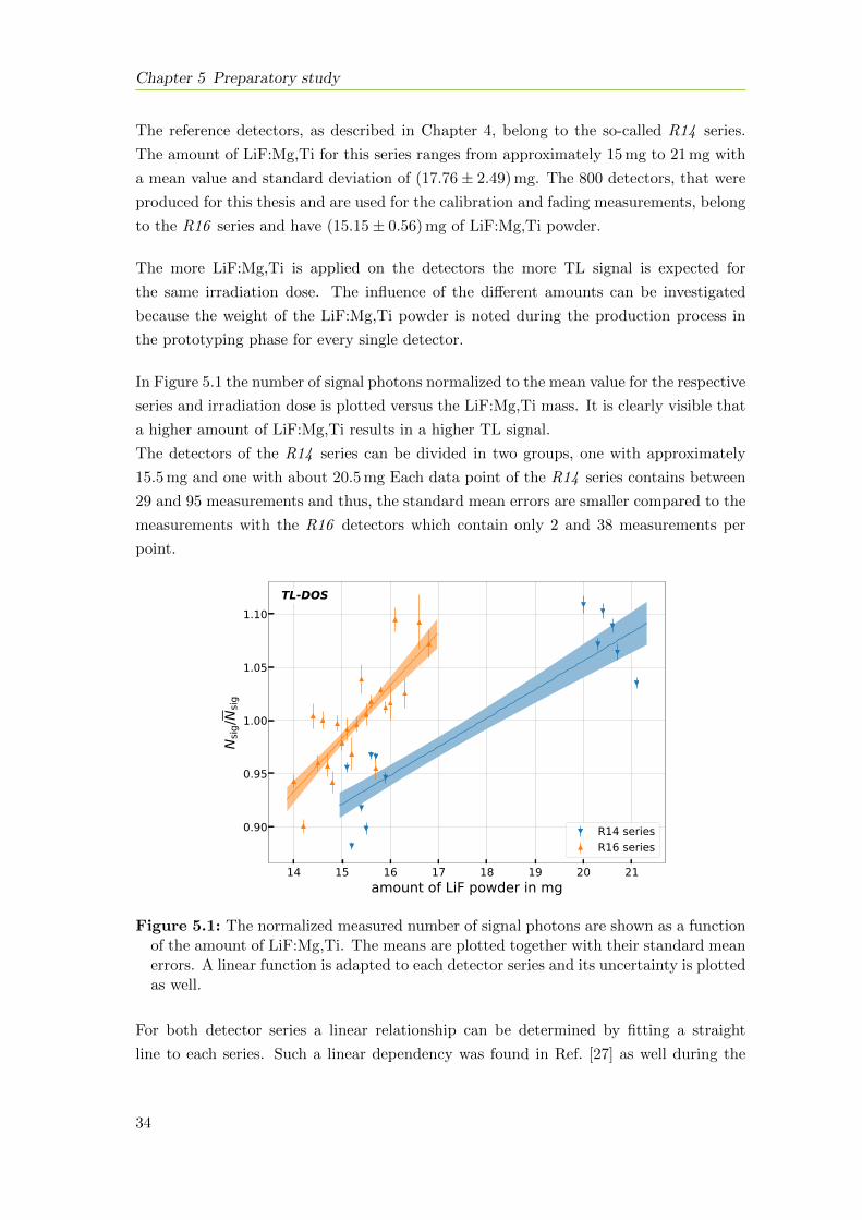
Chapter 5 Preparatory study
The reference detectors, as described in Chapter 4, belong to the so-called R14 series.
The amount of LiF:Mg,Ti for this series ranges from approximately 15 mg to 21 mg with
a mean value and standard deviation of (17.76± 2.49) mg. The 800 detectors, that were
produced for this thesis and are used for the calibration and fading measurements, belong
to the R16 series and have (15.15± 0.56) mg of LiF:Mg,Ti powder.
The more LiF:Mg,Ti is applied on the detectors the more TL signal is expected for
the same irradiation dose. The influence of the different amounts can be investigated
because the weight of the LiF:Mg,Ti powder is noted during the production process in
the prototyping phase for every single detector.
In Figure 5.1 the number of signal photons normalized to the mean value for the respective
series and irradiation dose is plotted versus the LiF:Mg,Ti mass. It is clearly visible that
a higher amount of LiF:Mg,Ti results in a higher TL signal.
The detectors of the R14 series can be divided in two groups, one with approximately
15.5 mg and one with about 20.5 mg Each data point of the R14 series contains between
29 and 95 measurements and thus, the standard mean errors are smaller compared to the
measurements with the R16 detectors which contain only 2 and 38 measurements per
point.
14 15 16 17 18 19 20 21amount of LiF powder in mg
0.90
0.95
1.00
1.05
1.10
Nsig
/ Nsig
R14 seriesR16 series
TL-DOS
Figure 5.1: The normalized measured number of signal photons are shown as a functionof the amount of LiF:Mg,Ti. The means are plotted together with their standard meanerrors. A linear function is adapted to each detector series and its uncertainty is plottedas well.
For both detector series a linear relationship can be determined by fitting a straight
line to each series. Such a linear dependency was found in Ref. [27] as well during the
34
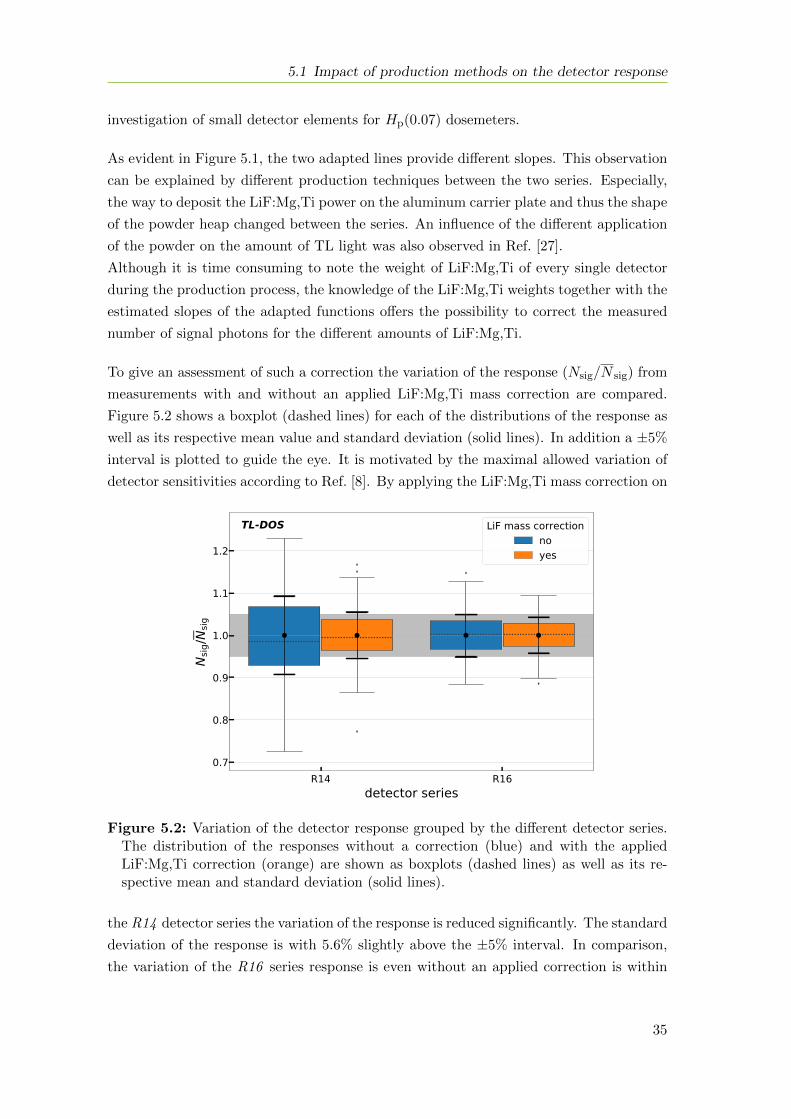
5.1 Impact of production methods on the detector response
investigation of small detector elements for Hp(0.07) dosemeters.
As evident in Figure 5.1, the two adapted lines provide different slopes. This observation
can be explained by different production techniques between the two series. Especially,
the way to deposit the LiF:Mg,Ti power on the aluminum carrier plate and thus the shape
of the powder heap changed between the series. An influence of the different application
of the powder on the amount of TL light was also observed in Ref. [27].
Although it is time consuming to note the weight of LiF:Mg,Ti of every single detector
during the production process, the knowledge of the LiF:Mg,Ti weights together with the
estimated slopes of the adapted functions offers the possibility to correct the measured
number of signal photons for the different amounts of LiF:Mg,Ti.
To give an assessment of such a correction the variation of the response (Nsig/N sig) from
measurements with and without an applied LiF:Mg,Ti mass correction are compared.
Figure 5.2 shows a boxplot (dashed lines) for each of the distributions of the response as
well as its respective mean value and standard deviation (solid lines). In addition a ±5%
interval is plotted to guide the eye. It is motivated by the maximal allowed variation of
detector sensitivities according to Ref. [8]. By applying the LiF:Mg,Ti mass correction on
R14 R16detector series
0.7
0.8
0.9
1.0
1.1
1.2
Nsig
/ Nsig
LiF mass correctionnoyes
TL-DOS
Figure 5.2: Variation of the detector response grouped by the different detector series.The distribution of the responses without a correction (blue) and with the appliedLiF:Mg,Ti correction (orange) are shown as boxplots (dashed lines) as well as its re-spective mean and standard deviation (solid lines).
the R14 detector series the variation of the response is reduced significantly. The standard
deviation of the response is with 5.6% slightly above the ±5% interval. In comparison,
the variation of the R16 series response is even without an applied correction is within
35
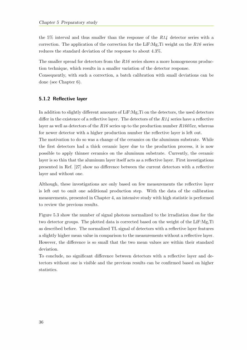
Chapter 5 Preparatory study
the 5% interval and thus smaller than the response of the R14 detector series with a
correction. The application of the correction for the LiF:Mg,Ti weight on the R16 series
reduces the standard deviation of the response to about 4.3%.
The smaller spread for detectors from the R16 series shows a more homogeneous produc-
tion technique, which results in a smaller variation of the detector response.
Consequently, with such a correction, a batch calibration with small deviations can be
done (see Chapter 6).
5.1.2 Reflective layer
In addition to slightly different amounts of LiF:Mg,Ti on the detectors, the used detectors
differ in the existence of a reflective layer. The detectors of the R14 series have a reflective
layer as well as detectors of the R16 series up to the production number R1605xx, whereas
for newer detector with a higher production number the reflective layer is left out.
The motivation to do so was a change of the ceramics on the aluminum substrate. While
the first detectors had a thick ceramic layer due to the production process, it is now
possible to apply thinner ceramics on the aluminum substrate. Currently, the ceramic
layer is so thin that the aluminum layer itself acts as a reflective layer. First investigations
presented in Ref. [27] show no difference between the current detectors with a reflective
layer and without one.
Although, these investigations are only based on few measurements the reflective layer
is left out to omit one additional production step. With the data of the calibration
measurements, presented in Chapter 4, an intensive study with high statistic is performed
to review the previous results.
Figure 5.3 show the number of signal photons normalized to the irradiation dose for the
two detector groups. The plotted data is corrected based on the weight of the LiF:Mg,Ti
as described before. The normalized TL signal of detectors with a reflective layer features
a slightly higher mean value in comparison to the measurements without a reflective layer.
However, the difference is so small that the two mean values are within their standard
deviation.
To conclude, no significant difference between detectors with a reflective layer and de-
tectors without one is visible and the previous results can be confirmed based on higher
statistics.
36
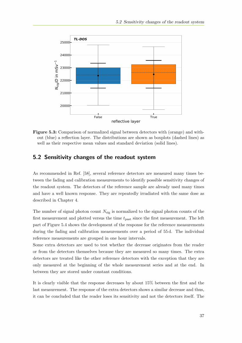
5.2 Sensitivity changes of the readout system
False Truereflective layer
20000
21000
22000
23000
24000
25000
Nsig
/D in
mSv
1
TL-DOS
Figure 5.3: Comparison of normalized signal between detectors with (orange) and with-out (blue) a reflection layer. The distributions are shown as boxplots (dashed lines) aswell as their respective mean values and standard deviation (solid lines).
5.2 Sensitivity changes of the readout system
As recommended in Ref. [58], several reference detectors are measured many times be-
tween the fading and calibration measurements to identify possible sensitivity changes of
the readout system. The detectors of the reference sample are already used many times
and have a well known response. They are repeatedly irradiated with the same dose as
described in Chapter 4.
The number of signal photon count Nsig is normalized to the signal photon counts of the
first measurement and plotted versus the time tpast since the first measurement. The left
part of Figure 5.4 shows the development of the response for the reference measurements
during the fading and calibration measurements over a period of 55 d. The individual
reference measurements are grouped in one hour intervals.
Some extra detectors are used to test whether the decrease originates from the reader
or from the detectors themselves because they are measured so many times. The extra
detectors are treated like the other reference detectors with the exception that they are
only measured at the beginning of the whole measurement series and at the end. In
between they are stored under constant conditions.
It is clearly visible that the response decreases by about 15% between the first and the
last measurement. The response of the extra detectors shows a similar decrease and thus,
it can be concluded that the reader loses its sensitivity and not the detectors itself. The
37
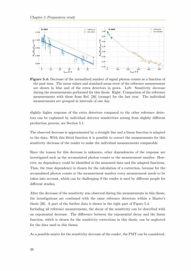
Chapter 5 Preparatory study
0 10 20 30 40 50tpast in d
0.85
0.90
0.95
1.00
1.05N
sig/N
sig(t p
ast=
0)referenceref. extra
TL-DOS
0 100 200 300 400 500tpast in d
0.3
0.4
0.5
0.6
0.7
0.8
0.9
1.0
Nsig
/Nsig
(t pas
t=0)
referenceref. Hantke
TL-DOS
Figure 5.4: Decrease of the normalized number of signal photon counts as a function ofthe past time. The mean values and standard mean error of the reference measurementare shown in blue and of the extra detectors in green. Left: Sensitivity decreaseduring the measurements performed for this thesis. Right: Comparison of the referencemeasurements with those from Ref. [26] (orange) for the last year. The individualmeasurements are grouped in intervals of one day.
slightly higher response of the extra detectors compared to the other reference detec-
tors can be explained by individual detector sensitivities arising from slightly different
production process, see Section 5.1.
The observed decrease is approximated by a straight line and a linear function is adapted
to the data. With this fitted function it is possible to correct the measurements for this
sensitivity decrease of the reader to make the individual measurements comparable.
Since the reason for this decrease is unknown, other dependencies of the response are
investigated such as the accumulated photon counts or the measurement number. How-
ever, no dependency could be identified in the measured data and the adapted functions.
Thus, the time dependency is chosen for the calculation of a correction, because for the
accumulated photon counts or the measurement number every measurement needs to be
taken into account, which can be challenging if the reader is used by different people for
different studies.
After the decrease of the sensitivity was observed during the measurements in this thesis,
the investigations are continued with the same reference detectors within a Master’s
thesis [26]. A part of the further data is shown in the right part of Figure 5.4.
Including all reference measurements, the decay of the sensitivity can be described with
an exponential decrease. The difference between the exponential decay and the linear
function, which is chosen for the sensitivity corrections in this thesis, can be neglected
for the data used in this theses.
As a possible source for the sensitivity decrease of the reader, the PMT can be considered.
38
5.3 Contribution of the natural radiation
For example, the vacuum quality could decreases or the release of electrons could cause
an aging of the PMT. However, none of these reasons can be clearly identified from the
data.
To conclude, a sensitivity decrease of the TL reader is found, but it is not yet finally un-
derstood and have to be investigated in more detail. Either way, the reference measure-
ments allow to correct for the sensitivity decrease and make the individual measurements
comparable.
5.3 Contribution of the natural radiation
For the fading measurements the detectors are stored after the irradiation until readout
for different times. During this time the detectors are permanently exposed to the natu-
ral radiation. The influence of the natural radiation on a measurement depends on the
irradiated dose as well as on the elapsed time between annealing and readout.
For most measurements, e.g. the calibration measurements described in Chapter 4, the
contribution of the natural radiation to the glow curve can be neglected since the accu-
mulated natural radiation dose is negligible compared to the dose from the irradiation.
However, the influence of the natural radiation has to be considered for the fading mea-
surements, especially for the 0.5 mSv measurements.
The left part of Figure 5.5 shows the impact of the natural radiation on the relative
decrease of the number of signal counts as a function of the fading time for two different
doses. In addition, the expected signal decrease due to thermal fading without contribu-
tion of natural radiation is plotted as a comparison.
It is expected that the number of signal counts decreases as a function of the fading time,
see dashed green line. However, the presence of natural radiation changes the shape of
the decrease and leads even to an increase of the relative number of signal counts for
an irradiation dose of 0.5 mSv. Whereas, the contribution of the natural radiation to an
irradiation of 10 mSv is nearly negligible.
To generate the plot the information of the fading time analysis of Chapter 6 and the
measured amount of natural radiation as a function of time, which is shown in Figure 5.6,
are used. The right part of Figure 5.5 shows the contribution of the natural radiation
to the number of measured photons as a function of the irradiation dose as well as the
time between annealing and readout. The brighter the color the less the measured counts
are influenced by the natural radiation. It is clearly visible that for irradiation doses
smaller than 1 mSv the contribution is higher than 10% for 40 d of fading. Therefore, it is
important to take the contribution of the natural radiation into account for the analysis
of the fading measurements.
39
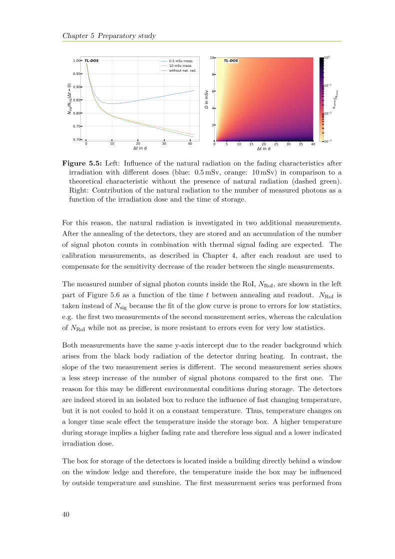
Chapter 5 Preparatory study
0 10 20 30 40t in d
0.70
0.75
0.80
0.85
0.90
0.95
1.00
Nsig
/Nsig
(t=
0)0.5 mSv meas10 mSv measwithout nat. rad.
TL-DOS
0 5 10 15 20 25 30 35 40t in d
2
4
6
8
10
D in
mSv
10 3
10 2
10 1
100
Nna
tRad
/ Nm
eas
TL-DOS
Figure 5.5: Left: Influence of the natural radiation on the fading characteristics afterirradiation with different doses (blue: 0.5 mSv, orange: 10 mSv) in comparison to atheoretical characteristic without the presence of natural radiation (dashed green).Right: Contribution of the natural radiation to the number of measured photons as afunction of the irradiation dose and the time of storage.
For this reason, the natural radiation is investigated in two additional measurements.
After the annealing of the detectors, they are stored and an accumulation of the number
of signal photon counts in combination with thermal signal fading are expected. The
calibration measurements, as described in Chapter 4, after each readout are used to
compensate for the sensitivity decrease of the reader between the single measurements.
The measured number of signal photon counts inside the RoI, NRoI, are shown in the left
part of Figure 5.6 as a function of the time t between annealing and readout. NRoI is
taken instead of Nsig because the fit of the glow curve is prone to errors for low statistics,
e.g. the first two measurements of the second measurement series, whereas the calculation
of NRoI while not as precise, is more resistant to errors even for very low statistics.
Both measurements have the same y-axis intercept due to the reader background which
arises from the black body radiation of the detector during heating. In contrast, the
slope of the two measurement series is different. The second measurement series shows
a less steep increase of the number of signal photons compared to the first one. The
reason for this may be different environmental conditions during storage. The detectors
are indeed stored in an isolated box to reduce the influence of fast changing temperature,
but it is not cooled to hold it on a constant temperature. Thus, temperature changes on
a longer time scale effect the temperature inside the storage box. A higher temperature
during storage implies a higher fading rate and therefore less signal and a lower indicated
irradiation dose.
The box for storage of the detectors is located inside a building directly behind a window
on the window ledge and therefore, the temperature inside the box may be influenced
by outside temperature and sunshine. The first measurement series was performed from
40
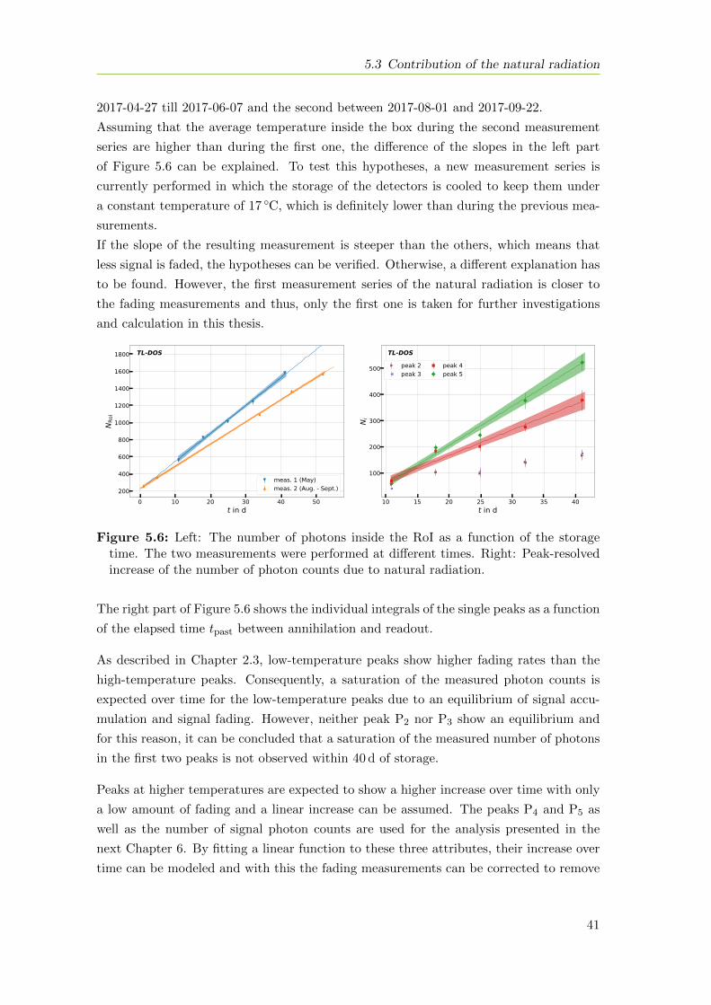
5.3 Contribution of the natural radiation
2017-04-27 till 2017-06-07 and the second between 2017-08-01 and 2017-09-22.
Assuming that the average temperature inside the box during the second measurement
series are higher than during the first one, the difference of the slopes in the left part
of Figure 5.6 can be explained. To test this hypotheses, a new measurement series is
currently performed in which the storage of the detectors is cooled to keep them under
a constant temperature of 17 ◦C, which is definitely lower than during the previous mea-
surements.
If the slope of the resulting measurement is steeper than the others, which means that
less signal is faded, the hypotheses can be verified. Otherwise, a different explanation has
to be found. However, the first measurement series of the natural radiation is closer to
the fading measurements and thus, only the first one is taken for further investigations
and calculation in this thesis.
0 10 20 30 40 50t in d
200
400
600
800
1000
1200
1400
1600
1800
NRo
I
meas. 1 (May)meas. 2 (Aug. - Sept.)
TL-DOS
10 15 20 25 30 35 40t in d
100
200
300
400
500N
ipeak 2peak 3
peak 4peak 5
TL-DOS
Figure 5.6: Left: The number of photons inside the RoI as a function of the storagetime. The two measurements were performed at different times. Right: Peak-resolvedincrease of the number of photon counts due to natural radiation.
The right part of Figure 5.6 shows the individual integrals of the single peaks as a function
of the elapsed time tpast between annihilation and readout.
As described in Chapter 2.3, low-temperature peaks show higher fading rates than the
high-temperature peaks. Consequently, a saturation of the measured photon counts is
expected over time for the low-temperature peaks due to an equilibrium of signal accu-
mulation and signal fading. However, neither peak P2 nor P3 show an equilibrium and
for this reason, it can be concluded that a saturation of the measured number of photons
in the first two peaks is not observed within 40 d of storage.
Peaks at higher temperatures are expected to show a higher increase over time with only
a low amount of fading and a linear increase can be assumed. The peaks P4 and P5 as
well as the number of signal photon counts are used for the analysis presented in the
next Chapter 6. By fitting a linear function to these three attributes, their increase over
time can be modeled and with this the fading measurements can be corrected to remove
41

Chapter 5 Preparatory study
the influence of the natural radiation for the fading time analysis. In contrast, for the
analysis in Chapter 7 no correction is applied to the data.
A further investigation of the natural radiation as a function of time can provide knowl-
edge about the irradiation dose accumulation during permanent irradiation and the be-
havior of the individual peaks, e.g. a possible saturation effect.
42
Chapter 6
Glow curve analysis with glow curve
deconvolution
The main quality of interest in dosimetry is to estimate the irradiation dose and thus, the
calibration process is investigated including an estimation of the uncertainties. If using
thermoluminescence (TL) dosemeters, the estimated irradiation dose depends on the time
between irradiation and the readout. Therefore, these fading influences on a glow curve
are investigated and a technique to estimate the fading time and correct the irradiation
dose for the fading is developed. Furthermore, the uncertainties on the fading time as
well as on the irradiation dose estimation from a faded glow curve are estimated.
The irradiation dose and its uncertainty estimation, based on a data set which was mea-
sured during a Master’s thesis [45], were already described in Ref. [3]. The fading time
and irradiation dose estimation of a faded glow curve were described in Ref. [4].
6.1 Calibration of the detectors
In this section a calibration function is determined with which an irradiation dose can be
estimated based on the number of measured photons. In addition, the uncertainties of
such a calibration are investigated as a function of the irradiation dose.
6.1.1 Determination of the calibration function
The nominal range of use for whole body dosemeters in personal routine dosimetry ranges
from 0.1 mSv to 1 Sv [8]. In this range the linear correlation between the measured pho-
ton counts and an irradiated dose, see Chapter 2.2, is used to give an estimate of the
irradiation dose.
To determine a calibration function and its uncertainties, measurements with different
43
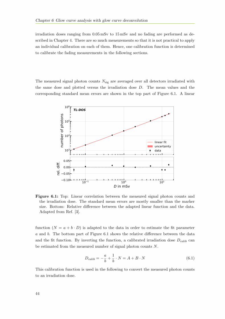
Chapter 6 Glow curve analysis with glow curve deconvolution
irradiation doses ranging from 0.05 mSv to 15 mSv and no fading are performed as de-
scribed in Chapter 4. There are so much measurements so that it is not practical to apply
an individual calibration on each of them. Hence, one calibration function is determined
to calibrate the fading measurements in the following sections.
The measured signal photon counts Nsig are averaged over all detectors irradiated with
the same dose and plotted versus the irradiation dose D. The mean values and the
corresponding standard mean errors are shown in the top part of Figure 6.1. A linear
103
104
105
106
num
ber o
f pho
tons
linear fituncertaintydata
10 1 100 101
D in mSv0.10
0.05
0.00
0.05
rel.
diff.
TL-DOS
Figure 6.1: Top: Linear correlation between the measured signal photon counts andthe irradiation dose. The standard mean errors are mostly smaller than the markersize. Bottom: Relative difference between the adapted linear function and the data.Adapted from Ref. [3].
function (N = a + b · D) is adapted to the data in order to estimate the fit parameter
a and b. The bottom part of Figure 6.1 shows the relative difference between the data
and the fit function. By inverting the function, a calibrated irradiation dose Dcalib can
be estimated from the measured number of signal photon counts N .
Dcalib = −ab
+1
b·N = A+B ·N (6.1)
This calibration function is used in the following to convert the measured photon counts
to an irradiation dose.
44
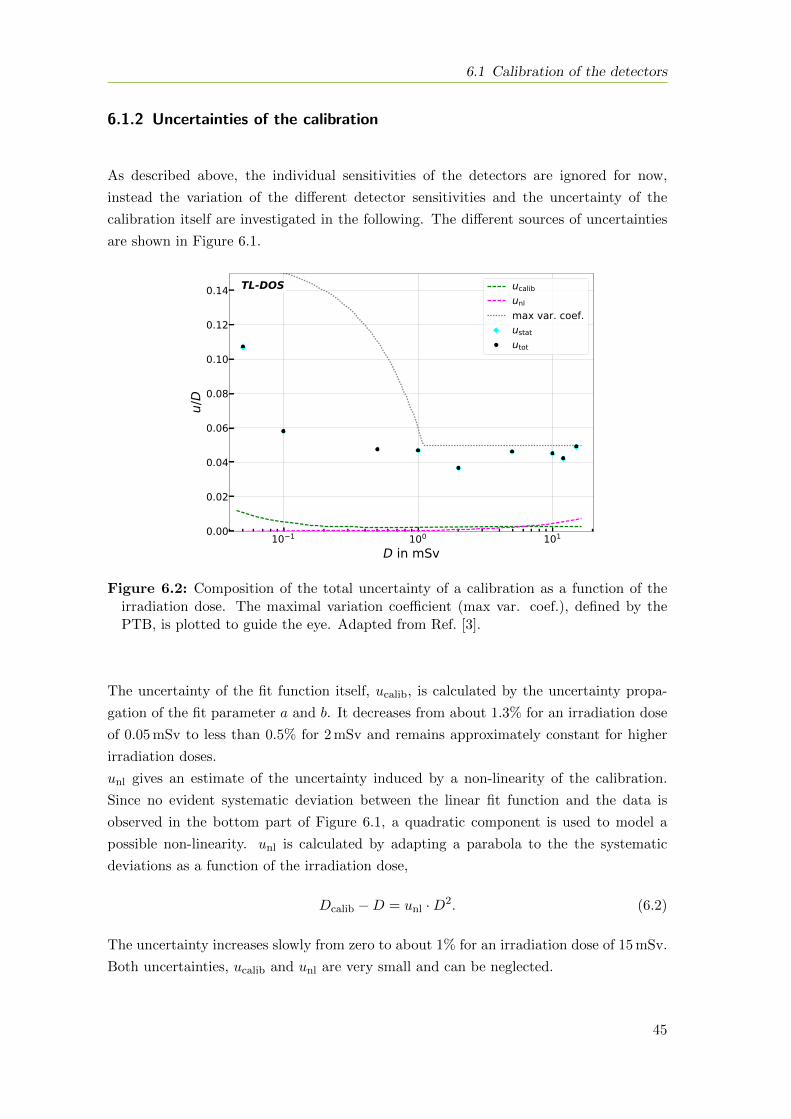
6.1 Calibration of the detectors
6.1.2 Uncertainties of the calibration
As described above, the individual sensitivities of the detectors are ignored for now,
instead the variation of the different detector sensitivities and the uncertainty of the
calibration itself are investigated in the following. The different sources of uncertainties
are shown in Figure 6.1.
10 1 100 101
D in mSv0.00
0.02
0.04
0.06
0.08
0.10
0.12
0.14
u/D
ucalibunlmax var. coef.ustatutot
TL-DOS
Figure 6.2: Composition of the total uncertainty of a calibration as a function of theirradiation dose. The maximal variation coefficient (max var. coef.), defined by thePTB, is plotted to guide the eye. Adapted from Ref. [3].
The uncertainty of the fit function itself, ucalib, is calculated by the uncertainty propa-
gation of the fit parameter a and b. It decreases from about 1.3% for an irradiation dose
of 0.05 mSv to less than 0.5% for 2 mSv and remains approximately constant for higher
irradiation doses.
unl gives an estimate of the uncertainty induced by a non-linearity of the calibration.
Since no evident systematic deviation between the linear fit function and the data is
observed in the bottom part of Figure 6.1, a quadratic component is used to model a
possible non-linearity. unl is calculated by adapting a parabola to the the systematic
deviations as a function of the irradiation dose,
Dcalib −D = unl ·D2. (6.2)
The uncertainty increases slowly from zero to about 1% for an irradiation dose of 15 mSv.
Both uncertainties, ucalib and unl are very small and can be neglected.
45
Chapter 6 Glow curve analysis with glow curve deconvolution
The variation of the different detector sensitivities is represented by the statistical un-
certainty ustat, which is estimated by the standard deviation σN of a sample of detectors
for each irradiation dose. The measured signal photon counts show a higher variation
for lower doses, about 11% for an irradiation dose of 0.05 mSv, due to less statistics. For
higher irradiation doses the statistical deviation decreases to a bit less than 5%.
The total uncertainty utot is the quadratic sum of the three contributions ucalib, unl and
ustat. It is clearly visible that ustat has the highest contribution to total uncertainty
utot, but nevertheless it is lower than the maximal variation coefficient for whole body
dosemeters in personal routine, specified by the PTB [8].
It should be mentioned that an individual calibration of each detector, as performed in
individual dosimetry, should lower ustat, whereas unl and ucalib are unaffected.
6.2 Fading time estimation
The measured irradiation dose by a dosemeter is influenced by the effect of fading. If the
fading characteristics of the used material and the fading time are known, the estimated
irradiation dose can be corrected for the signal decrease due to fading [59, 60].
In routine dosimetry a possible irradiation date and, consequently, the fading time are
usually unknown. However, to be able to estimate an accurate irradiation dose, the
estimation can be derived from the high-temperature peaks. For this purpose there are
two approaches.
On the one hand, by applying a pre-heating technique as described in Chapter 2.4.3 the
highly fading time dependent low-temperature peaks are erased and the remaining TL
signal is mostly independent of the elapsed time between irradiation and readout [23, 22].
On the other hand, if the whole glow curve is read out, a GCD can be applied or a
suitable RoI can be set as in Ref. [61] to limit the irradiation dose estimation to the
high-temperature peaks, which makes the estimated irradiation dose independent of any
fading time influences.
All these methods have in common that they reduce the overall signal strength and
remove possible information about the irradiation itself. In the following an alternative
approach is presented to estimate the fading time directly from the glow curve.
6.2.1 A possible estimator for the fading time
The estimation of the fading time takes the different impact of the fading on the indi-
vidual glow peaks into account. Due to the different half-lifes of the peaks, described in
46
6.2 Fading time estimation
Chapter 2.3, the ratio of two peak contents changes during the time between irradiation
and readout and therefore, it can be used as an estimator. The single peak contents are
obtained from the GCD.
Peak ratios were already used in the past to estimate the fading time, e.g. the ratio
P3/P5 is used for the fading time investigation of a LiF:Mg,Ti detector [62]. In addition,
peak ratios are also used for the fading time analysis of CaSO4:Dy and LiF:Mg,Cu,P
detectors [63, 64].
In comparison to the commonly used linear heating rates, the heating rates during expo-
nential heating are very high and therefore, it is difficult to separate especially the glow
peaks P4 and P5 in a GCD, because they are highly overlapping. Furthermore, both glow
peaks show a similar fading rate over the investigated fading time range. Consequently,
the sum of both peaks (N4 +N5) is used in the following analysis to avoid the influence
of peak overlap in GCD.
To estimate the fading time the fading ratio F is defined as the sum of the photon counts
in the fourth and fifths glow peaks divided by the number signal photon counts Nsig. As
shown in Figure 6.3, the fading ratio F is a non-linear function of the fading time ∆t.
In the figure the data of the four different investigated irradiation doses, 0.5 mSv, 1 mSv,
5 mSv and 10 mSv, is averaged over certain fading time intervals and the means are
plotted together with their standard mean errors. F increases from 0.60, directly after
the irradiation (∆t = 0), up to 0.87 for more than 40 d of fading. For higher fading
times the increase becomes more gently inclined compared to the steep increase at the
beginning.
Equation (6.3) is a simple empiric parameterization to describe the trend of the non-linear
correlation between F and ∆t.
F (∆t) = A ·√
∆t+B ·∆t+ C (6.3)
The fit parameter A, B and C depend on the used detectors as well as on the environ-
mental conditions during the storage. The presented parameterization has less parameter
compared to Ref. [63] and only one quantity is needed to describe the fading in contrast
to Ref. [62] where two quantities (one for short- and one for long-time fading) are used.
By computing F and solving Equation (6.3) for ∆t the fading time can be estimated
up to at least five weeks. For longer fading time F diverges and the parameterization
deviates from the data.
47
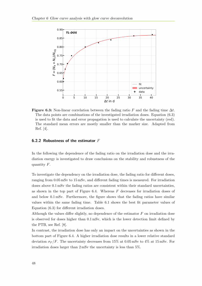
Chapter 6 Glow curve analysis with glow curve deconvolution
0 5 10 15 20 25 30 35 40t in d
0.55
0.60
0.65
0.70
0.75
0.80
0.85
0.90
F=
(N4
+N
5)/N
sig
fituncertaintydata
TL-DOS
Figure 6.3: Non-linear correlation between the fading ratio F and the fading time ∆t.The data points are combinations of the investigated irradiation doses. Equation (6.3)is used to fit the data and error propagation is used to calculate the uncertainty (red).The standard mean errors are mostly smaller than the marker size. Adapted fromRef. [4].
6.2.2 Robustness of the estimator F
In the following the dependence of the fading ratio on the irradiation dose and the irra-
diation energy is investigated to draw conclusions on the stability and robustness of the
quantity F .
To investigate the dependency on the irradiation dose, the fading ratio for different doses,
ranging from 0.05 mSv to 15 mSv, and different fading times is measured. For irradiation
doses above 0.1 mSv the fading ratios are consistent within their standard uncertainties,
as shown in the top part of Figure 6.4. Whereas F decreases for irradiation doses of
and below 0.1 mSv. Furthermore, the figure shows that the fading ratios have similar
values within the same fading time. Table 6.1 shows the best fit parameter values of
Equation (6.3) for different irradiation doses.
Although the values differ slightly, no dependence of the estimator F on irradiation dose
is observed for doses higher than 0.1 mSv, which is the lower detection limit defined by
the PTB, see Ref. [8].
In contrast, the irradiation dose has only an impact on the uncertainties as shown in the
bottom part of Figure 6.4. A higher irradiation dose results in a lower relative standard
deviation σF /F . The uncertainty decreases from 15% at 0.05 mSv to 4% at 15 mSv. For
irradiation doses larger than 2 mSv the uncertainty is less than 5%.
48
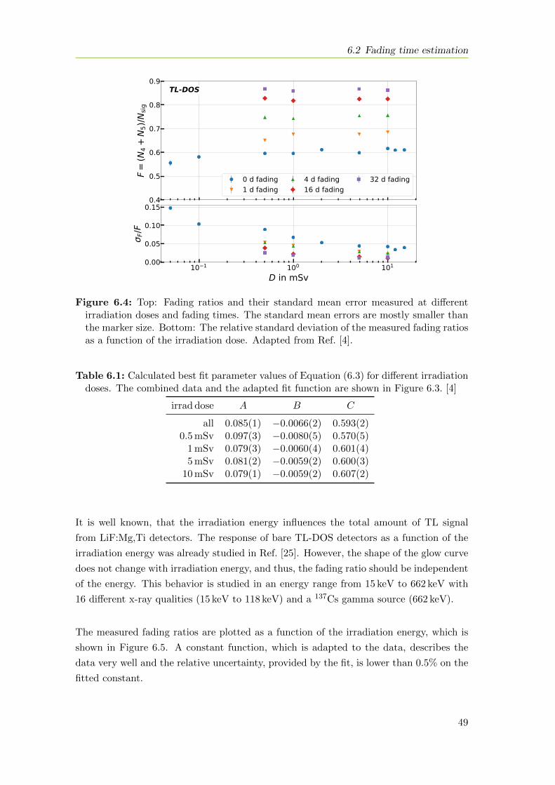
6.2 Fading time estimation
0.4
0.5
0.6
0.7
0.8
0.9
F=
(N4
+N
5)/N
sig
0 d fading1 d fading
4 d fading16 d fading
32 d fading
10 1 100 101
D in mSv0.00
0.05
0.10
0.15
F/F
TL-DOS
Figure 6.4: Top: Fading ratios and their standard mean error measured at differentirradiation doses and fading times. The standard mean errors are mostly smaller thanthe marker size. Bottom: The relative standard deviation of the measured fading ratiosas a function of the irradiation dose. Adapted from Ref. [4].
Table 6.1: Calculated best fit parameter values of Equation (6.3) for different irradiationdoses. The combined data and the adapted fit function are shown in Figure 6.3. [4]
irrad dose A B C
all 0.085(1) −0.0066(2) 0.593(2)0.5 mSv 0.097(3) −0.0080(5) 0.570(5)
1 mSv 0.079(3) −0.0060(4) 0.601(4)5 mSv 0.081(2) −0.0059(2) 0.600(3)
10 mSv 0.079(1) −0.0059(2) 0.607(2)
It is well known, that the irradiation energy influences the total amount of TL signal
from LiF:Mg,Ti detectors. The response of bare TL-DOS detectors as a function of the
irradiation energy was already studied in Ref. [25]. However, the shape of the glow curve
does not change with irradiation energy, and thus, the fading ratio should be independent
of the energy. This behavior is studied in an energy range from 15 keV to 662 keV with
16 different x-ray qualities (15 keV to 118 keV) and a 137Cs gamma source (662 keV).
The measured fading ratios are plotted as a function of the irradiation energy, which is
shown in Figure 6.5. A constant function, which is adapted to the data, describes the
data very well and the relative uncertainty, provided by the fit, is lower than 0.5% on the
fitted constant.
49
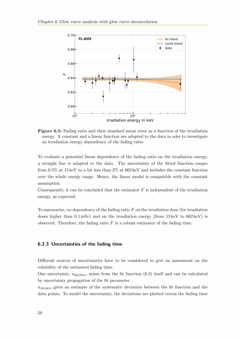
Chapter 6 Glow curve analysis with glow curve deconvolution
101 102
irradiation energy in keV
0.60
0.62
0.64
0.66
0.68
0.70
F
lin trendconst trenddata
TL-DOS
Figure 6.5: Fading ratio and their standard mean error as a function of the irradiationenergy. A constant and a linear function are adapted to the data in oder to investigatean irradiation energy dependency of the fading ratio.
To evaluate a potential linear dependence of the fading ratio on the irradiation energy,
a straight line is adapted to the data. The uncertainty of the fitted function ranges
from 0.5% at 15 keV to a bit less than 2% at 662 keV and includes the constant function
over the whole energy range. Hence, the linear model is compatible with the constant
assumption.
Consequently, it can be concluded that the estimator F is independent of the irradiation
energy, as expected.
To summarize, no dependency of the fading ratio F on the irradiation dose (for irradiation
doses higher than 0.1 mSv) and on the irradiation energy (from 15 keV to 662 keV) is
observed. Therefore, the fading ratio F is a robust estimator of the fading time.
6.2.3 Uncertainties of the fading time
Different sources of uncertainties have to be considered to give an assessment on the
reliability of the estimated fading time.
One uncertainty, u∆t;func, arises from the fit function (6.3) itself and can be calculated
by uncertainty propagation of the fit parameter.
u∆t;devi gives an estimate of the systematic deviation between the fit function and the
data points. To model the uncertainty, the deviations are plotted versus the fading time
50
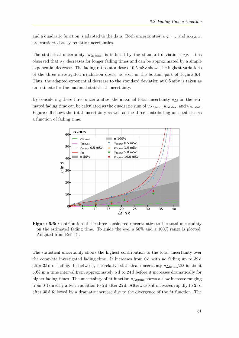
6.2 Fading time estimation
and a quadratic function is adapted to the data. Both uncertainties, u∆t;func and u∆t;devi,
are considered as systematic uncertainties.
The statistical uncertainty, u∆t;stat, is induced by the standard deviations σF . It is
observed that σF decreases for longer fading times and can be approximated by a simple
exponential decrease. The fading ratios at a dose of 0.5 mSv shows the highest variations
of the three investigated irradiation doses, as seen in the bottom part of Figure 6.4.
Thus, the adapted exponential decrease to the standard deviation at 0.5 mSv is taken as
an estimate for the maximal statistical uncertainty.
By considering these three uncertainties, the maximal total uncertainty u∆t on the esti-
mated fading time can be calculated as the quadratic sum of u∆t;func, u∆t;devi and u∆t;stat.
Figure 6.6 shows the total uncertainty as well as the three contributing uncertainties as
a function of fading time.
0 5 10 15 20 25 30 35 40t in d
0
10
20
30
40
50
60
u in
d
u t; deviu t; funcu t; stat 0.5 mSvu t
± 50%
± 100%u t; stat 0.5 mSvu t; stat 1.0 mSvu t; stat 5.0 mSvu t; stat 10.0 mSv
TL-DOS
Figure 6.6: Contribution of the three considered uncertainties to the total uncertaintyon the estimated fading time. To guide the eye, a 50% and a 100% range is plotted.Adapted from Ref. [4].
The statistical uncertainty shows the highest contribution to the total uncertainty over
the complete investigated fading time. It increases from 0 d with no fading up to 39 d
after 35 d of fading. In between, the relative statistical uncertainty u∆t;stat/∆t is about
50% in a time interval from approximately 5 d to 24 d before it increases dramatically for
higher fading times. The uncertainty of fit function u∆t;func shows a slow increase ranging
from 0 d directly after irradiation to 5 d after 25 d. Afterwards it increases rapidly to 25 d
after 35 d followed by a dramatic increase due to the divergence of the fit function. The
51
Chapter 6 Glow curve analysis with glow curve deconvolution
contribution of the systematic deviation u∆t;devi can be neglected, it increases from 0 d
to just about 3.5 d after 40 d.
As seen in Subsection 6.2.1 the estimator F diverges for longer fading times resulting
in a large uncertainty for fading time higher than 34 d. This dramatic increase of the
uncertainty for longer fading time is mostly driven by u∆t;stat and u∆t;func, whereas the
systematic deviation is not affected by the divergence of the parameterization.
In spite of the dramatic increase, the total uncertainty is about 50% for fading times
between 5 d and 25 d and smaller than 100% for fading times up to 34 d. Afterwards
no reliable prediction can be made. Therefore, the presented estimator can be used to
estimate the fading time to 34 d, which is a sufficient time interval in individual routine
dose monitoring.
6.3 Irradiation dose estimation with fading influences
In individual dose monitoring, the knowledge about the time of irradiation is a useful
additional information, but it is much more important to know the irradiation dose
itself.
Due to the loss of TL signal during fading it is difficult to estimate an unbiased irradiation
dose. However, the additional information of the elapsed time since irradiation, as de-
scribed in the previous section, can be used to correct the measured signal photon counts
and estimate a fading time independent irradiation dose. Such a technique is presented
in the following.
6.3.1 Initial photon counts estimation
The relative decrease of the signal strength is irradiation dose independent and can be
described by
frel =Nt(∆t)
N0, (6.4)
where N0 is the number of signal photon counts directly after the irradiation and Nt(∆t)
the fading time dependent number of signal photons.
Figure 6.7 shows the development of signal strength as a function of the fading time. The
relative number of signal photons decreases from 1 to 0.7 within 40 d after irradiation.
After a rapid loss of TL signal at the beginning, the decrease becomes smaller for longer
52
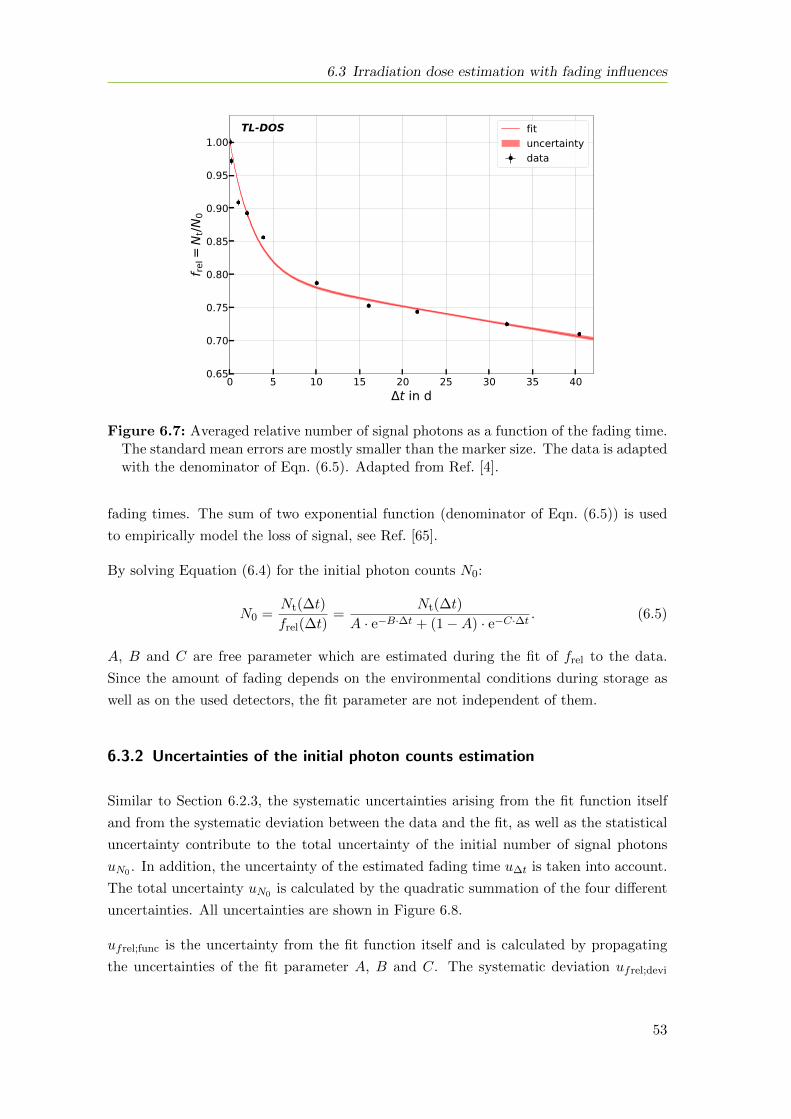
6.3 Irradiation dose estimation with fading influences
0 5 10 15 20 25 30 35 40t in d
0.65
0.70
0.75
0.80
0.85
0.90
0.95
1.00
f rel=
Nt/N
0
fituncertaintydata
TL-DOS
Figure 6.7: Averaged relative number of signal photons as a function of the fading time.The standard mean errors are mostly smaller than the marker size. The data is adaptedwith the denominator of Eqn. (6.5). Adapted from Ref. [4].
fading times. The sum of two exponential function (denominator of Eqn. (6.5)) is used
to empirically model the loss of signal, see Ref. [65].
By solving Equation (6.4) for the initial photon counts N0:
N0 =Nt(∆t)
frel(∆t)=
Nt(∆t)
A · e−B·∆t + (1−A) · e−C·∆t. (6.5)
A, B and C are free parameter which are estimated during the fit of frel to the data.
Since the amount of fading depends on the environmental conditions during storage as
well as on the used detectors, the fit parameter are not independent of them.
6.3.2 Uncertainties of the initial photon counts estimation
Similar to Section 6.2.3, the systematic uncertainties arising from the fit function itself
and from the systematic deviation between the data and the fit, as well as the statistical
uncertainty contribute to the total uncertainty of the initial number of signal photons
uN0 . In addition, the uncertainty of the estimated fading time u∆t is taken into account.
The total uncertainty uN0 is calculated by the quadratic summation of the four different
uncertainties. All uncertainties are shown in Figure 6.8.
ufrel;func is the uncertainty from the fit function itself and is calculated by propagating
the uncertainties of the fit parameter A, B and C. The systematic deviation ufrel;devi
53
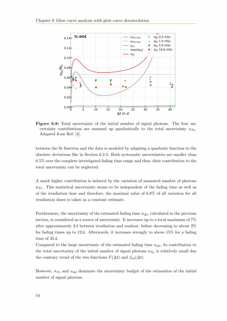
Chapter 6 Glow curve analysis with glow curve deconvolution
0 5 10 15 20 25 30 35 40t in d
0.00
0.02
0.04
0.06
0.08
0.10
0.12
0.14
N0/N
0
ufrel; funcufrel; deviu t
max( Nt)uN0
Nt 0.5 mSvNt 1.0 mSvNt 5.0 mSvNt 10.0 mSv
TL-DOS
Figure 6.8: Total uncertainty of the initial number of signal photons. The four un-certainty contributions are summed up quadratically to the total uncertainty uN0 .Adapted from Ref. [4].
between the fit function and the data is modeled by adapting a quadratic function to the
absolute deviations like in Section 6.2.3. Both systematic uncertainties are smaller than
0.5% over the complete investigated fading time range and thus, their contribution to the
total uncertainty can be neglected.
A much higher contribution is induced by the variation of measured number of photons
σNt. This statistical uncertainty seems to be independent of the fading time as well as
of the irradiation dose and therefore, the maximal value of 6.8% of all variation for all
irradiation doses is taken as a constant estimate.
Furthermore, the uncertainty of the estimated fading time u∆t, calculated in the previous
section, is considered as a source of uncertainty. It increases up to a local maximum of 7%
after approximately 2 d between irradiation and readout, before decreasing to about 2%
for fading times up to 12 d. Afterwards, it increases strongly to above 15% for a fading
time of 35 d.
Compared to the large uncertainty of the estimated fading time u∆t, its contribution to
the total uncertainty of the initial number of signal photons uN0 is relatively small due
the contrary trend of the two functions F (∆t) and frel(∆t).
However, σNt and u∆t dominate the uncertainty budget of the estimation of the initial
number of signal photons.
54
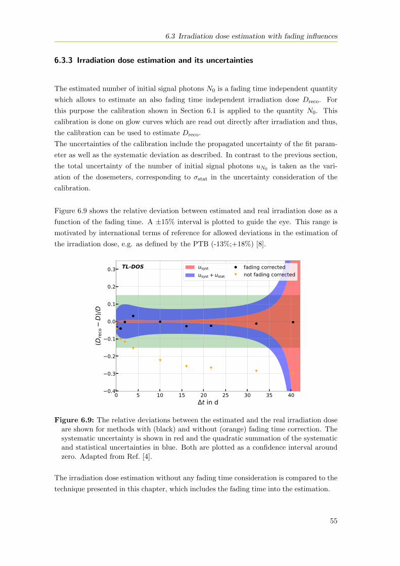
6.3 Irradiation dose estimation with fading influences
6.3.3 Irradiation dose estimation and its uncertainties
The estimated number of initial signal photons N0 is a fading time independent quantity
which allows to estimate an also fading time independent irradiation dose Dreco. For
this purpose the calibration shown in Section 6.1 is applied to the quantity N0. This
calibration is done on glow curves which are read out directly after irradiation and thus,
the calibration can be used to estimate Dreco.
The uncertainties of the calibration include the propagated uncertainty of the fit param-
eter as well as the systematic deviation as described. In contrast to the previous section,
the total uncertainty of the number of initial signal photons uN0 is taken as the vari-
ation of the dosemeters, corresponding to σstat in the uncertainty consideration of the
calibration.
Figure 6.9 shows the relative deviation between estimated and real irradiation dose as a
function of the fading time. A ±15% interval is plotted to guide the eye. This range is
motivated by international terms of reference for allowed deviations in the estimation of
the irradiation dose, e.g. as defined by the PTB (-13%;+18%) [8].
0 5 10 15 20 25 30 35 40t in d
0.4
0.3
0.2
0.1
0.0
0.1
0.2
0.3
(Dre
coD
)/D
usystusyst + ustat
fading correctednot fading corrected
TL-DOS
Figure 6.9: The relative deviations between the estimated and the real irradiation doseare shown for methods with (black) and without (orange) fading time correction. Thesystematic uncertainty is shown in red and the quadratic summation of the systematicand statistical uncertainties in blue. Both are plotted as a confidence interval aroundzero. Adapted from Ref. [4].
The irradiation dose estimation without any fading time consideration is compared to the
technique presented in this chapter, which includes the fading time into the estimation.
55
Chapter 6 Glow curve analysis with glow curve deconvolution
Without any fading time correction, the deviations between the estimated and the real
irradiation dose are already higher than 10% after 3 d and after 5 d they are outside the
specified ±15% range. Whereas the relative deviations of the estimation considering the
fading time are smaller than 5% over the whole investigated fading time and thus, they
are clearly inside ±15% range.
The systematic deviation is about 1% for fading times up to 15 d. Afterwards it rises
slowly, followed by a dramatical increase after 35 d. The statistical uncertainty dominates
the total uncertainty up to about 25 d of fading. For longer fading time the systematic
uncertainty contributes very considerably to the total uncertainty of the estimated irra-
diation dose. Including all investigated uncertainties, the uncertainty of the estimated
irradiation dose is within the defined range up to approximately 34 d and for fading times
shorter than 30 d it is even smaller than 10%.
Due to the dramatic increase for longer fading times it is not possible to give a reliable
estimation for fading times longer than approximately 34 d with the presented functions.
However, an estimation of an upper limit of the irradiation dose is always possible, due
to the known time between annealing and readout, the maximal possible fading time. In
this way the point at approximately 40 d is reconstructed.
It can be concluded that the presented technique, including all investigated uncertainties,
guarantees a reliable irradiation dose estimation inside a ±15% range for fading times
up to five weeks which is a very likely time span for routine dosimetry. Furthermore,
it is clearly visible that the total uncertainty on the irradiation dose is mostly driven
by the systematic uncertainty of the estimator F which is induced by its divergence for
longer fading times and thus, a non diverging method is desirable. A possible approach
to reduce the systematic uncertainty is a multivariate analysis, which is investigated in
the next chapter.
In addition, scenarios with multiple irradiations are investigated [66, 56]. Furthermore,
the influence of the time between annealing and irradiation is investigated in Ref. [67].
56

Chapter 7
Glow curve analysis with machine learning
As shown in Chapter 6, it is possible to estimate the fading time and the irradiation dose
of a faded glow curve. However, the constructed fading ratio F diverged for longer fading
times resulting in a large uncertainty, see Figure 6.6. This makes predictions not reliable
for fading times greater than 34 d.
In order to reduce the uncertainty of the prediction for even longer fading times, more
information is needed. The additional information is provided by other characteristics of
the glow curve, also referred to as features.
The idea of a multivariate analysis (MVA) is to combine multiple features to calculate
the prediction output. For this calculation a multitude of machine learning algorithms
are available.
In this chapter the capability of a shallow neural network to predict the fading time as
well as the irradiation dose of a faded glow curve is investigated.
7.1 Basics of machine learning
In machine learning, tasks can be distinguished into three categories, namely supervised,
unsupervised and reinforcement learning. In all tasks the inputs of a learner are called
features, independent variables or predictors.
The prediction of a known quantity, e.g. the fading time, belongs to the category of su-
pervised learning. During the supervised learning, a predictive model is trained on data
samples with known output, also referred to as targets or dependent variables. The model
is then used to predict the target for an unknown data set. The other two categories are
discussed for example in Refs. [68, 69, 70].
In supervised learning, a distinction is drawn between classification and regression. Ap-
plications, in which the input samples are divided into different classes are referred to
57
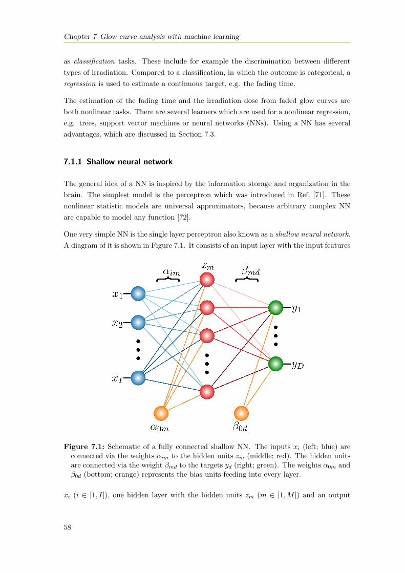
Chapter 7 Glow curve analysis with machine learning
as classification tasks. These include for example the discrimination between different
types of irradiation. Compared to a classification, in which the outcome is categorical, a
regression is used to estimate a continuous target, e.g. the fading time.
The estimation of the fading time and the irradiation dose from faded glow curves are
both nonlinear tasks. There are several learners which are used for a nonlinear regression,
e.g. trees, support vector machines or neural networks (NNs). Using a NN has several
advantages, which are discussed in Section 7.3.
7.1.1 Shallow neural network
The general idea of a NN is inspired by the information storage and organization in the
brain. The simplest model is the perceptron which was introduced in Ref. [71]. These
nonlinear statistic models are universal approximators, because arbitrary complex NN
are capable to model any function [72].
One very simple NN is the single layer perceptron also known as a shallow neural network.
A diagram of it is shown in Figure 7.1. It consists of an input layer with the input features
Figure 7.1: Schematic of a fully connected shallow NN. The inputs xi (left; blue) areconnected via the weights αim to the hidden units zm (middle; red). The hidden unitsare connected via the weight βmd to the targets yd (right; green). The weights α0m andβ0d (bottom; orange) represents the bias units feeding into every layer.
xi (i ∈ [1, I]), one hidden layer with the hidden units zm (m ∈ [1,M ]) and an output
58
7.1 Basics of machine learning
layer with the targets yd (d ∈ [1, D]).
Generally, it is possible to have more than one hidden layer in a NN. In this example,
each input unit is connected to every hidden unit and each hidden unit is connected
to every output target. It is therefore a so-called fully-connected neural network. This
two-stage model can be used for classification as well as for regression. In the first stage,
M new features, the so-called hidden units zm, are calculated as linear combinations of
the input features xi. The zm have the form
zm = h
(α0m +
I∑i=1
αimxi
), (7.1)
where I is the number of input feature and h is an activation function, e.g. sigmoid or
hyperbolic tangent function.
To estimate the D different targets yd, linear combination of the hidden units zm are
used. This can be done with Equation (7.2), where σ is also an activation function which
may be another than h:
yd = σ
(β0d +
M∑m=1
βmdzm
). (7.2)
The weights αim and βmd as well as the bias units α0m and β0d are calculated during the
training process, which is done by minimizing a loss or error function.
The activation functions belong to the so-called hyperparameter which define the model
of a machine learning algorithm. Other examples of hyperparameter of a shallow NN are
the solver, which optimizes the weights during the fit process, or the number of hidden
units M .
7.1.2 Model selection and assessment
The accuracy in future predictions is one of the major assessment criteria for a machine
learning algorithm. To estimate the prediction performance, the learner is trained first
and afterwards the prediction performance is tested. Using the same data set for training
and testing, no generalization error can be estimated.
To avoid a wrong assessment and to get access to a good estimate of the predictive
performance on unseen data, the data set can be split in a training and a test data set.
The training data set is used, as the name suggests, to train the estimator and the test
data set is used to estimate the learners generalization performance. As a consequence,
the prediction performance, also referred to as score s, is estimated on data, which the
learner does not see during the training process and accordingly does not know.
59
Chapter 7 Glow curve analysis with machine learning
If the prediction performance on the test set is much lower than on the training set, the
generalization performance is low, which is an indication for over-training. To reduce the
effect of over-training and achieve a higher generalization performance, many learners use
regularization.
One way to gain more generalization strength is to add a penalty term, e.g. L2 regular-
ization, to the loss function of a regression function.
Loss(ypred, ytrue, ω) =1
2||ypred − ytrue||22 +
α
2||ω||22, (7.3)
where ypred is the predicted target, ytrue the true target, α the regularization strength
and ω the weights in the NN.
In addition to the model assessment, one of the main goals in machine learning is the
model selection. Finding the best performing model includes the search for the best set
of hyperparameter of a learner, as well as the comparison of different learners. Figure 7.2
shows the used approach to estimate the set of hyperparameter, for which the learner
achieves the best prediction performance.
During the so-called grid-search, the performance of a learner with different parameter
combinations (set 1 to set j) is estimated in order to find the best set. To avoid the
influence of over-training on the selection of the best set, the training data is split again
in a validation and a training set. With sufficient data statistics, the additional splitting
has no impact on the performance, but for data sets with low statistics the validation set
might be very small, which results in a relatively noisy estimate of the performance.
To counter this and still give a good estimate of the generalization performance, a cross-
validation is performed. In a cross-validation the validation set is much smaller compared
to the training set and the model is trained and validated multiple times on different parts
of the data set so that more than one part of the data is used for validation.
In a K-fold cross-validation, the data is split in K equally parts, also referred to as folds.
The model is trained on K−1 folds of the data and the remaining part is used to predict
the learners performance. By altering the different folds which are used for training and
validation, K scores can be estimated. The average score smean of all single validation
scores sj gives a good estimate of the learners performance.
By comparing the validation and training scores, an estimate about over-training can be
made as well. The less both scores differ the more reliable is the performance estimate
of the learner to unseen data. In the reality, often a trade-off between a high score and
a low bias between both scores has to be found.
The major drawback of a cross-validation is that the number of fitting and predicting
processes increases by a factor of K and thus, the computing time increases also with a
60
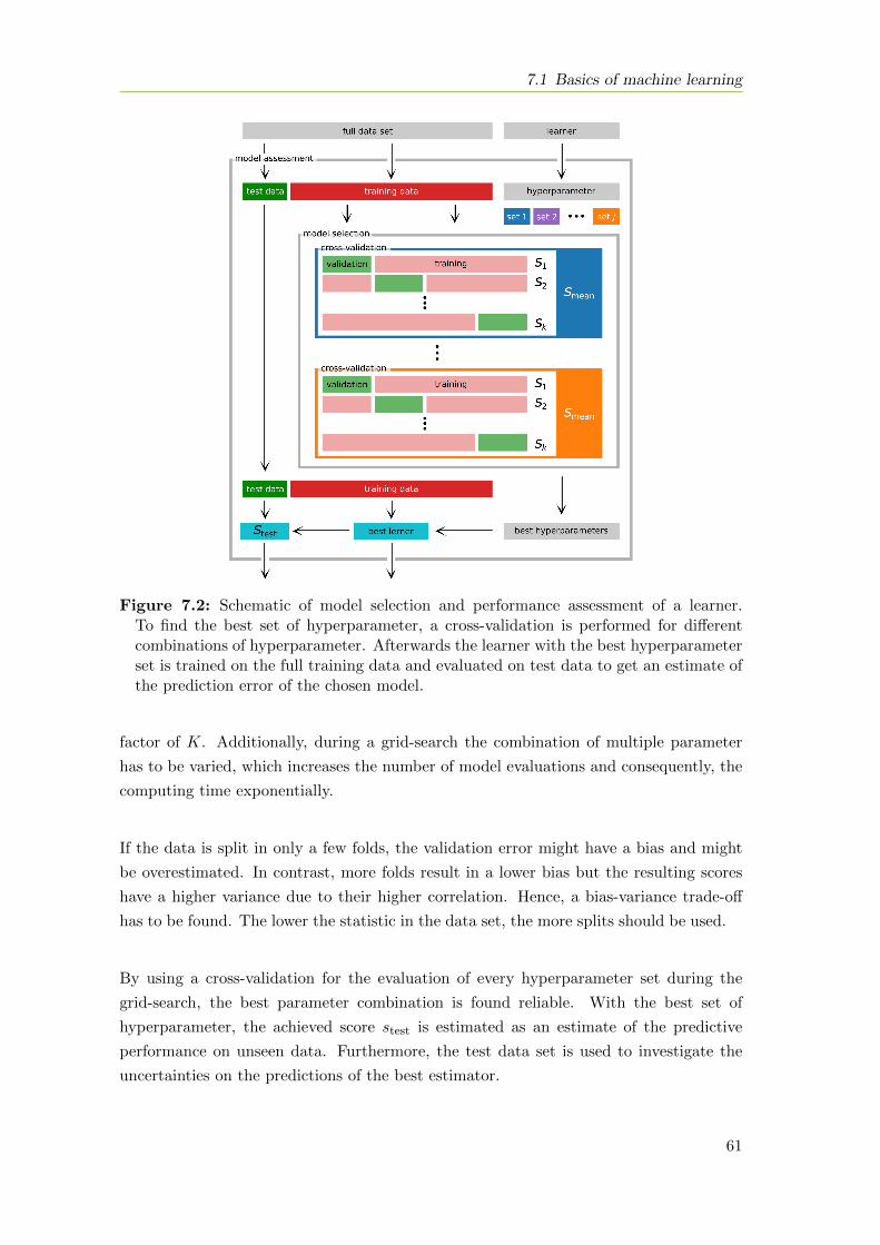
7.1 Basics of machine learning
Figure 7.2: Schematic of model selection and performance assessment of a learner.To find the best set of hyperparameter, a cross-validation is performed for differentcombinations of hyperparameter. Afterwards the learner with the best hyperparameterset is trained on the full training data and evaluated on test data to get an estimate ofthe prediction error of the chosen model.
factor of K. Additionally, during a grid-search the combination of multiple parameter
has to be varied, which increases the number of model evaluations and consequently, the
computing time exponentially.
If the data is split in only a few folds, the validation error might have a bias and might
be overestimated. In contrast, more folds result in a lower bias but the resulting scores
have a higher variance due to their higher correlation. Hence, a bias-variance trade-off
has to be found. The lower the statistic in the data set, the more splits should be used.
By using a cross-validation for the evaluation of every hyperparameter set during the
grid-search, the best parameter combination is found reliable. With the best set of
hyperparameter, the achieved score stest is estimated as an estimate of the predictive
performance on unseen data. Furthermore, the test data set is used to investigate the
uncertainties on the predictions of the best estimator.
61
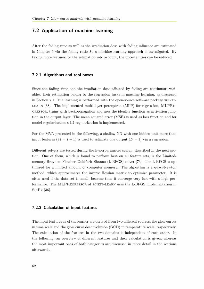
Chapter 7 Glow curve analysis with machine learning
7.2 Application of machine learning
After the fading time as well as the irradiation dose with fading influence are estimated
in Chapter 6 via the fading ratio F , a machine learning approach is investigated. By
taking more features for the estimation into account, the uncertainties can be reduced.
7.2.1 Algorithms and tool boxes
Since the fading time and the irradiation dose affected by fading are continuous vari-
ables, their estimation belong to the regression tasks in machine learning, as discussed
in Section 7.1. The learning is performed with the open-source software package scikit-
learn [38]. The implemented multi-layer perceptron (MLP) for regression, MLPRe-
gressor, trains with backpropagation and uses the identity function as activation func-
tion in the output layer. The mean squared error (MSE) is used as loss function and for
model regularization a L2 regularization is implemented.
For the MVA presented in the following, a shallow NN with one hidden unit more than
input features (M = I + 1) is used to estimate one output (D = 1) via a regression.
Different solvers are tested during the hyperparameter search, described in the next sec-
tion. One of them, which is found to perform best on all feature sets, is the Limited-
memory Broyden–Fletcher–Goldfarb–Shanno (L-BFGS) solver [73]. The L-BFGS is op-
timized for a limited amount of computer memory. The algorithm is a quasi-Newton
method, which approximates the inverse Hessian matrix to optimize parameter. It is
often used if the data set is small, because then it converge very fast with a high per-
formance. The MLPRegressor of scikit-learn uses the L-BFGS implementation in
SciPy [36].
7.2.2 Calculation of input features
The input features xi of the learner are derived from two different sources, the glow curves
in time scale and the glow curve deconvolution (GCD) in temperature scale, respectively.
The calculation of the features in the two domains is independent of each other. In
the following, an overview of different features and their calculation is given, whereas
the most important ones of both categories are discussed in more detail in the sections
afterwards.
62
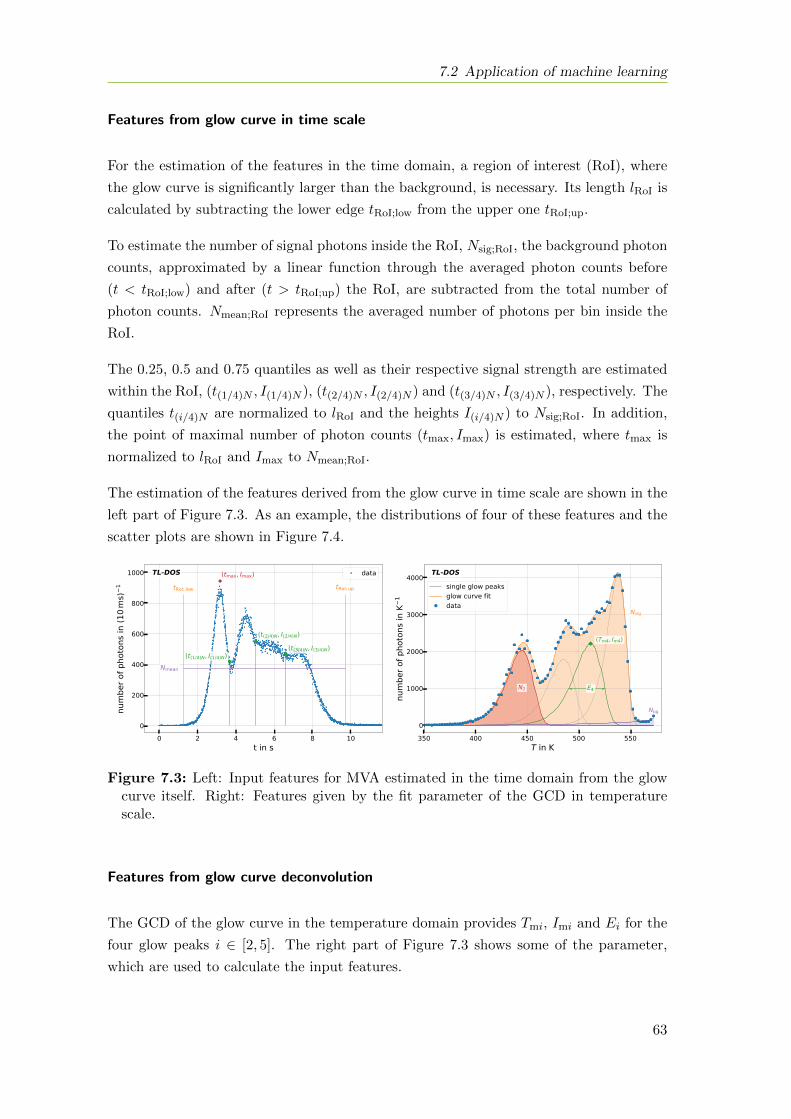
7.2 Application of machine learning
Features from glow curve in time scale
For the estimation of the features in the time domain, a region of interest (RoI), where
the glow curve is significantly larger than the background, is necessary. Its length lRoI is
calculated by subtracting the lower edge tRoI;low from the upper one tRoI;up.
To estimate the number of signal photons inside the RoI, Nsig;RoI, the background photon
counts, approximated by a linear function through the averaged photon counts before
(t < tRoI;low) and after (t > tRoI;up) the RoI, are subtracted from the total number of
photon counts. Nmean;RoI represents the averaged number of photons per bin inside the
RoI.
The 0.25, 0.5 and 0.75 quantiles as well as their respective signal strength are estimated
within the RoI, (t(1/4)N , I(1/4)N ), (t(2/4)N , I(2/4)N ) and (t(3/4)N , I(3/4)N ), respectively. The
quantiles t(i/4)N are normalized to lRoI and the heights I(i/4)N ) to Nsig;RoI. In addition,
the point of maximal number of photon counts (tmax, Imax) is estimated, where tmax is
normalized to lRoI and Imax to Nmean;RoI.
The estimation of the features derived from the glow curve in time scale are shown in the
left part of Figure 7.3. As an example, the distributions of four of these features and the
scatter plots are shown in Figure 7.4.
(tmax, Imax)
0 2 4 6 8 10t in s
0
200
400
600
800
1000
num
ber o
f pho
tons
in (1
0ms)
1 tRoI; low tRoI; up
(t(1/4)N, I(1/4)N)
(t(2/4)N, I(2/4)N)(t(3/4)N, I(3/4)N)
data
Nmean
TL-DOS
350 400 450 500 550T in K
0
1000
2000
3000
4000
num
ber o
f pho
tons
in K
1
Nbg
Nsig
(Tm4, Im4)
E4N2
single glow peaksglow curve fitdata
TL-DOS
Figure 7.3: Left: Input features for MVA estimated in the time domain from the glowcurve itself. Right: Features given by the fit parameter of the GCD in temperaturescale.
Features from glow curve deconvolution
The GCD of the glow curve in the temperature domain provides Tmi, Imi and Ei for the
four glow peaks i ∈ [2, 5]. The right part of Figure 7.3 shows some of the parameter,
which are used to calculate the input features.
63
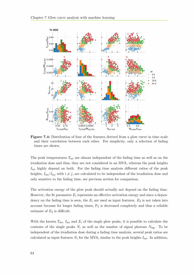
Chapter 7 Glow curve analysis with machine learning
0.4
0.6
0.8
t (1/4
)N/l R
oI
0.002
0.004
0.006
I (2/4
)N/N
sig;R
oI
1
2
3
t RoI
;low
t0 d2 d16 d41 d
0.50 0.75t(1/4)N/lRoI
0.3
0.4
Nm
ean/I
max
0.0025 0.0050I(2/4)N/Nsig; RoI
1 2 3tRoI; low
0.3 0.4Nmean/Imax
TL-DOS
Figure 7.4: Distribution of four of the features derived from a glow curve in time scaleand their correlation between each other. For simplicity, only a selection of fadingtimes are shown.
The peak temperatures Tmi are almost independent of the fading time as well as on the
irradiation dose and thus, they are not considered in an MVA, whereas the peak heights
Imi highly depend on both. For the fading time analysis different ratios of the peak
heights, Imi/Imj with i 6= j, are calculated to be independent of the irradiation dose and
only sensitive to the fading time, see previous section for comparison.
The activation energy of the glow peak should actually not depend on the fading time.
However, the fit parameter Ei represents an effective activation energy and since a depen-
dency on the fading time is seen, the Ei are used as input features. E2 is not taken into
account because for longer fading times, P2 is decreased completely and thus a reliable
estimate of E2 is difficult.
With the known Tmi, Imi and Ei of the single glow peaks, it is possible to calculate the
contents of the single peaks Ni as well as the number of signal photons Nsig. To be
independent of the irradiation dose during a fading time analysis, several peak ratios are
calculated as input features Ni for the MVA, similar to the peak heights Imi. In addition,
64
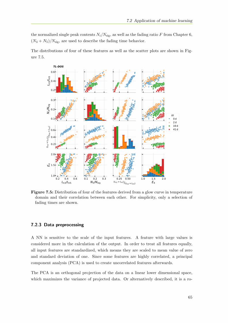
7.2 Application of machine learning
the normalized single peak contents Ni/Nsig, as well as the fading ratio F from Chapter 6,
(N4 +N5)/Nsig, are used to describe the fading time behavior.
The distributions of four of these features as well as the scatter plots are shown in Fig-
ure 7.5.
0.2
0.4
0.6
I m3/I
m5
0.1
0.2
0.3
N3/N
sig
0.2
0.4
0.6
(I m2
+I m
3)/ (I m
4+
I m5)
t0 d2 d16 d41 d
0.2 0.4 0.6Im3/Im5
1.0
1.5
2.0
E 4
0.1 0.2 0.3N3/Nsig
0.25 0.50(Im2 + Im3)/(Im4 + Im5)
1.0 1.5 2.0E4
TL-DOS
Figure 7.5: Distribution of four of the features derived from a glow curve in temperaturedomain and their correlation between each other. For simplicity, only a selection offading times are shown.
7.2.3 Data preprocessing
A NN is sensitive to the scale of the input features. A feature with large values is
considered more in the calculation of the output. In order to treat all features equally,
all input features are standardized, which means they are scaled to mean value of zero
and standard deviation of one. Since some features are highly correlated, a principal
component analysis (PCA) is used to create uncorrelated features afterwards.
The PCA is an orthogonal projection of the data on a linear lower dimensional space,
which maximizes the variance of projected data. Or alternatively described, it is a ro-
65
Chapter 7 Glow curve analysis with machine learning
tation of the coordinate system, where the new coordinate axis minimizes the distance
between data points and new axis. Both definitions lead to the same result. The esti-
mated new features are called principal components and are unique with the exception
of the sign. They are linearly uncorrelated, i.e. they have a unit covariance matrix, and
are sorted by decreasing variance.
The explained variance ratio is measure of how much percentage of the total variance
is caused by a the single component. By taking only the components with the highest
explained variance ratio into account, the dimension of the data can be reduces without
losing too much information. Thus, a PCA is not only used for feature decorrelation,
but also for dimensionality reduction or feature extraction. However, as the projection
is unsupervised the first principal components are not necessarily the most important
features for a certain target. This needs to be considered if components are neglected in
supervised learning.
7.2.4 Hyperparameter search
For the studies in the following sections, a grid-search is performed each time in order
to find the best hyperparameter of a learner. The different hyperparameter sets are
evaluated by calculating the averaged negative MSE (score) of the validation set in an
8-fold cross-validation.
The hyperparameter of the shallow NN which are varied during the grid-search is the
activation function h, the strength of regularization L2 and the solver. Four activation
functions are tested: the identity function (h(x) = x), the sigmoid function (h(x) =
1/(1 + exp(−x))), the hyperbolic tangent function (h(x) = tanh(x)) and the rectified
linear unit function (h(x) = max(0, x)). The relative strength of the penalty term of the
L2 regularization is varied in a wide range between 10−6 and 102.
Finally, the performances of the L-BFGS, the stochastic gradient decent (SGD) and an
ADAM solver are compared. ADAM stands for adaptive moment estimation and the
solver is an expansion of a stochastic gradient-based optimizer [74]. Individual adaptive
learning rates are used for the parameter optimization, which is done by estimating the
first and second moments of the gradients. The ADAM solver performs well on large data
sets with regard to time and score. Each of the solvers has several individual parameter,
which define the specific update process of the weights and are varied in the grid-search
as well.
In total, more than 39 000 different hyperparameter sets are tested in order to find the
best learner.
66
7.3 Fading time estimation
7.3 Fading time estimation
For the estimation of the fading time ∆t with an NN, the same data set is used as for the
estimation in Chapter 6.2.1 in order to make a fair comparison. As shown in Table 4.1,
the fading data set consists of four different irradiation doses with ten fading times.
However, the data is not corrected for the natural radiation as in Chapter 6, because it
is not possible to correct all input features for this. In addition, it is expected that a
machine learning algorithm is less prone to such influences.
The test set is obtained by splitting 10% of the total data, using stratified sampling,
which results in equally distributed fading time and irradiation dose combination in the
data sets. The test set is used to evaluate the performance and estimate the uncertainties
of the final learner.
The remaining 90% of the total data set are used to select a feature set, find the best
hyperparameter and to study the over-training and robustness of the final learner. In
each of the validation steps, the learner is thus trained on 79% and validated on about
11% of the total data set.
7.3.1 Feature selection
Four different feature sets are tested in order to compare their performances and find a
robust set to estimate the fading time. Since the number of features differs between the
single sets, the corresponding NNs differ in their complexity, because the number of units
in the hidden layer (M = I + 1) is one more than the number of input features I.
For each feature set a grid-search is performed. A NN with a L-BFGS solver using
a hyperbolic tangent as the activation function in the hidden nodes achieves the best
performance on each of the four feature sets.
The first feature set contains only features that can be extracted from the glow curve
without any fit or transformation. This feature set is independent of a GCD and contains
11 different features. It is not expected that this feature set performs as good as feature
sets which contain features extracted by GCD, but it is taken into account to assess the
performance of a NN which is independent of a previous fit or transformation.
The features of the second set are all obtained from the GCD of the glow curve after
transforming it to the temperature domain. It contains 25 features which include different
combinations of peak height ratios and peak integral ratios, as described in Section 7.2.2.
In addition Ei is also included in the feature set. The feature set is tested to estimate
the performance gain of the learner by using information from the separated glow peaks
instead of the total curve.
67
Chapter 7 Glow curve analysis with machine learning
The third feature set combines all features from the first and second feature set. With
its 36 features, it contains all information obtained from the glow curve in time domain
and from the GCD in the temperature domain. A learner, which used all available
information, is expected to provide the best performance. However, such a high number
of features results in a large number of weights in a fully connected NN. If the number
of events in the data set is in the same order of magnitude as the number of weights, an
over-training of the learner is more likely.
The fourth feature set is a subset of all features. The selection includes the most impor-
tant features of four feature groups, namely the first feature set, all peak height ratios,
all peak integral ratios and Ei, respectively. If two features within one feature group are
highly correlated among each other, only one of them is used.
For longer fading times, peak P2 is almost completely decreased and neither E2 nor N2
can be estimated reliable. Consequently, the integral of the second peak is not considered.
In contrast to E2, the height of the peak at a given temperature can be estimated more
reliable and thus, I2 is taken into account.
Following this procedure, seven features are selected. Since the features come from differ-
ent types of group, the fourth feature set is expected to result in a good performance.
The MSE of the training as well as of the validation set using an 8-fold cross-validation
are shown in Figure 7.6 for each of the four feature sets. The MSEs are calculated with
the best hyperparameter set resulting from the grid-search.
With the first feature set a training and validation score using the MSE of s =−0.024(1)
and s =−0.042(8), respectively is achieved. The offset between both scores indicates that
there is a slight over-training. Furthermore, the validation score shows a high variation
between the different splits of the cross-validation. Both, the offset and the high varia-
tion suggest that the information of the glow curve without any fit or transformation is
insufficient for a reliable fading time estimation.
Although, the grid-search results in a much higher regularization (α = 1) for the second
feature set compared to the first one (α = 0.0001), the training and validation score of
the second set are higher than those of the first one. Since the scores agree with each
other within their uncertainties, s =−0.018(1) and s =−0.020(2), there are no hints for
an over-training. Hence, it can be concluded that the features obtained from the GCD
are better to predict the fading time than those of the glow curve in the time domain.
As expected, the third feature set achieves the highest training score, s =−0.013(1), of
all tested feature sets. However, the validation score of s =−0.018(3) is similar to that of
the second feature set. Furthermore, the training process with more than thirty features
takes twice as long as for the second feature set.
68
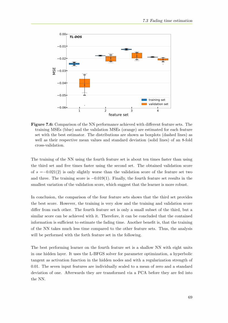
7.3 Fading time estimation
1 2 3 4feature set
0.06
0.05
0.04
0.03
0.02
0.01
0.00
MSE
training setvalidation set
TL-DOS
Figure 7.6: Comparison of the NN performance achieved with different feature sets. Thetraining MSEs (blue) and the validation MSEs (orange) are estimated for each featureset with the best estimator. The distributions are shown as boxplots (dashed lines) aswell as their respective mean values and standard deviation (solid lines) of an 8-foldcross-validation.
The training of the NN using the fourth feature set is about ten times faster than using
the third set and five times faster using the second set. The obtained validation score
of s =−0.021(2) is only slightly worse than the validation score of the feature set two
and three. The training score is −0.019(1). Finally, the fourth feature set results in the
smallest variation of the validation score, which suggest that the learner is more robust.
In conclusion, the comparison of the four feature sets shows that the third set provides
the best score. However, the training is very slow and the training and validation score
differ from each other. The fourth feature set is only a small subset of the third, but a
similar score can be achieved with it. Therefore, it can be concluded that the contained
information is sufficient to estimate the fading time. Another benefit is, that the training
of the NN takes much less time compared to the other feature sets. Thus, the analysis
will be performed with the forth feature set in the following.
The best performing learner on the fourth feature set is a shallow NN with eight units
in one hidden layer. It uses the L-BFGS solver for parameter optimization, a hyperbolic
tangent as activation function in the hidden nodes and with a regularization strength of
0.01. The seven input features are individually scaled to a mean of zero and a standard
deviation of one. Afterwards they are transformed via a PCA before they are fed into
the NN.
69
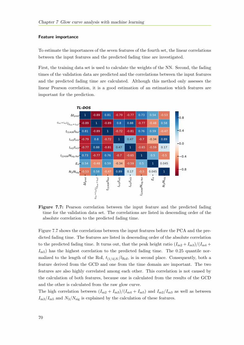
Chapter 7 Glow curve analysis with machine learning
Feature importance
To estimate the importances of the seven features of the fourth set, the linear correlations
between the input features and the predicted fading time are investigated.
First, the training data set is used to calculate the weights of the NN. Second, the fading
times of the validation data are predicted and the correlations between the input features
and the predicted fading time are calculated. Although this method only assesses the
linear Pearson correlation, it is a good estimation of an estimation which features are
important for the prediction.
t pre
d
(I m2
+I m
3)/ (I m
4+
I m5)
t (1/4
)N/l R
oI
I m3/I
m5
I m2/I
m3
I (2/4
)N/N
sig;R
oI E 4
N3/N
sig
tpred
(Im2 + Im3)/(Im4 + Im5)
t(1/4)N/lRoI
Im3/Im5
Im2/Im3
I(2/4)N/Nsig; RoI
E4
N3/Nsig
1 -0.89 0.81 -0.79 -0.77 0.73 0.54 -0.53
-0.89 1 -0.89 0.8 0.88 -0.77 -0.48 0.58
0.81 -0.89 1 -0.72 -0.81 0.76 0.59 -0.47
-0.79 0.8 -0.72 1 0.47 -0.7 -0.34 0.89
-0.77 0.88 -0.81 0.47 1 -0.65 -0.59 0.17
0.73 -0.77 0.76 -0.7 -0.65 1 0.5 -0.5
0.54 -0.48 0.59 -0.34 -0.59 0.5 1 0.045
-0.53 0.58 -0.47 0.89 0.17 -0.5 0.045 1 0.8
0.4
0.0
0.4
0.8
TL-DOSTL-DOS
Figure 7.7: Pearson correlation between the input feature and the predicted fadingtime for the validation data set. The correlations are listed in descending order of theabsolute correlation to the predicted fading time.
Figure 7.7 shows the correlations between the input features before the PCA and the pre-
dicted fading time. The features are listed in descending order of the absolute correlation
to the predicted fading time. It turns out, that the peak height ratio (Im2 + Im3)/(Im4 +
Im5) has the highest correlation to the predicted fading time. The 0.25 quantile nor-
malized to the length of the RoI, t(1/4)N/lRoI, is in second place. Consequently, both a
feature derived from the GCD and one from the time domain are important. The two
features are also highly correlated among each other. This correlation is not caused by
the calculation of both features, because one is calculated from the results of the GCD
and the other is calculated from the raw glow curve.
The high correlation between (Im2 + Im3)/(Im4 + Im5) and Im2/Im3 as well as between
Im3/Im5 and N3/Nsig is explained by the calculation of these features.
70
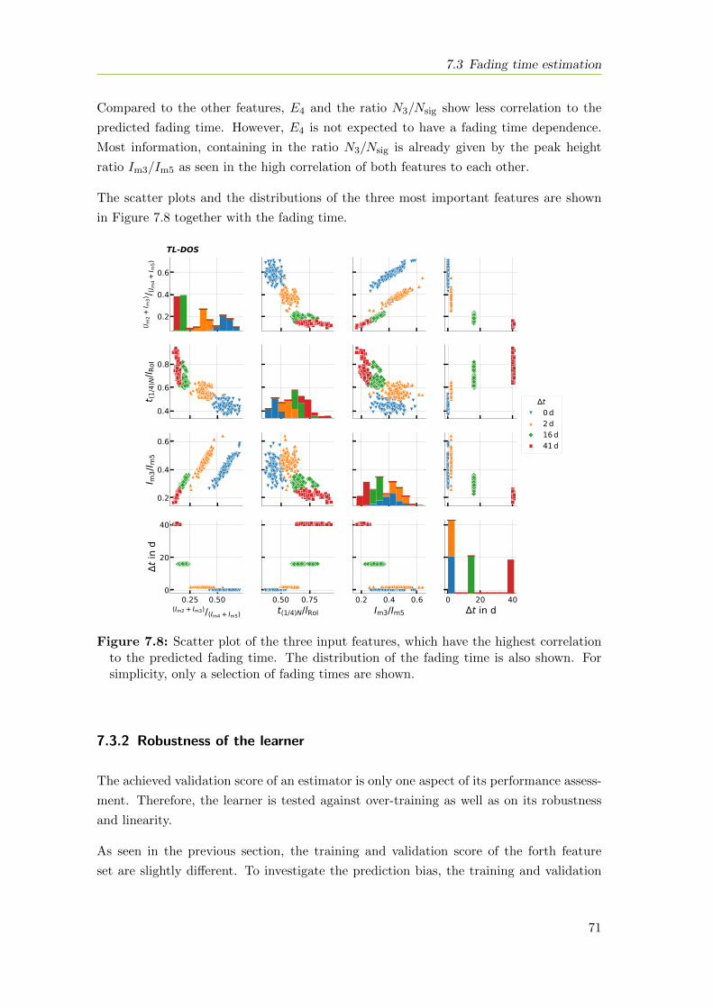
7.3 Fading time estimation
Compared to the other features, E4 and the ratio N3/Nsig show less correlation to the
predicted fading time. However, E4 is not expected to have a fading time dependence.
Most information, containing in the ratio N3/Nsig is already given by the peak height
ratio Im3/Im5 as seen in the high correlation of both features to each other.
The scatter plots and the distributions of the three most important features are shown
in Figure 7.8 together with the fading time.
0.2
0.4
0.6
(I m2
+I m
3)/ (I m
4+
I m5)
0.4
0.6
0.8
t (1/4
)N/l R
oI
0.2
0.4
0.6
I m3/I
m5
t0 d2 d16 d41 d
0.25 0.50(Im2 + Im3)/(Im4 + Im5)
0
20
40
t in
d
0.50 0.75t(1/4)N/lRoI
0.2 0.4 0.6Im3/Im5
0 20 40t in d
TL-DOS
Figure 7.8: Scatter plot of the three input features, which have the highest correlationto the predicted fading time. The distribution of the fading time is also shown. Forsimplicity, only a selection of fading times are shown.
7.3.2 Robustness of the learner
The achieved validation score of an estimator is only one aspect of its performance assess-
ment. Therefore, the learner is tested against over-training as well as on its robustness
and linearity.
As seen in the previous section, the training and validation score of the forth feature
set are slightly different. To investigate the prediction bias, the training and validation
71
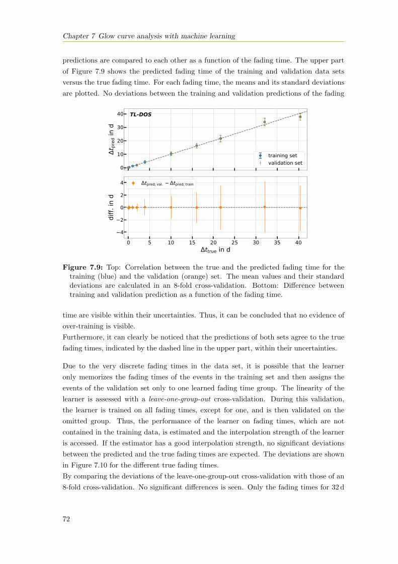
Chapter 7 Glow curve analysis with machine learning
predictions are compared to each other as a function of the fading time. The upper part
of Figure 7.9 shows the predicted fading time of the training and validation data sets
versus the true fading time. For each fading time, the means and its standard deviations
are plotted. No deviations between the training and validation predictions of the fading
0
10
20
30
40t p
red i
n d
training setvalidation set
0 5 10 15 20 25 30 35 40ttrue in d
4
2
0
2
4
diff.
in d
tpred; val. tpred; train
TL-DOS
Figure 7.9: Top: Correlation between the true and the predicted fading time for thetraining (blue) and the validation (orange) set. The mean values and their standarddeviations are calculated in an 8-fold cross-validation. Bottom: Difference betweentraining and validation prediction as a function of the fading time.
time are visible within their uncertainties. Thus, it can be concluded that no evidence of
over-training is visible.
Furthermore, it can clearly be noticed that the predictions of both sets agree to the true
fading times, indicated by the dashed line in the upper part, within their uncertainties.
Due to the very discrete fading times in the data set, it is possible that the learner
only memorizes the fading times of the events in the training set and then assigns the
events of the validation set only to one learned fading time group. The linearity of the
learner is assessed with a leave-one-group-out cross-validation. During this validation,
the learner is trained on all fading times, except for one, and is then validated on the
omitted group. Thus, the performance of the learner on fading times, which are not
contained in the training data, is estimated and the interpolation strength of the learner
is accessed. If the estimator has a good interpolation strength, no significant deviations
between the predicted and the true fading times are expected. The deviations are shown
in Figure 7.10 for the different true fading times.
By comparing the deviations of the leave-one-group-out cross-validation with those of an
8-fold cross-validation. No significant differences is seen. Only the fading times for 32 d
72
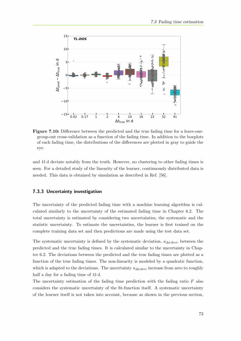
7.3 Fading time estimation
0.02 0.17 1 2 4 10 16 22 32 41ttrue in d
15
10
5
0
5
10
15
t pre
dt tr
ue in
d
TL-DOS
Figure 7.10: Difference between the predicted and the true fading time for a leave-one-group-out cross-validation as a function of the fading time. In addition to the boxplotsof each fading time, the distributions of the differences are plotted in gray to guide theeye.
and 41 d deviate notably from the truth. However, no clustering to other fading times is
seen. For a detailed study of the linearity of the learner, continuously distributed data is
needed. This data is obtained by simulation as described in Ref. [56].
7.3.3 Uncertainty investigation
The uncertainty of the predicted fading time with a machine learning algorithm is cal-
culated similarly to the uncertainty of the estimated fading time in Chapter 6.2. The
total uncertainty is estimated by considering two uncertainties, the systematic and the
statistic uncertainty. To estimate the uncertainties, the learner is first trained on the
complete training data set and then predictions are made using the test data set.
The systematic uncertainty is defined by the systematic deviation, u∆t;devi, between the
predicted and the true fading times. It is calculated similar to the uncertainty in Chap-
ter 6.2. The deviations between the predicted and the true fading times are plotted as a
function of the true fading times. The non-linearity is modeled by a quadratic function,
which is adapted to the deviations. The uncertainty u∆t;devi increase from zero to roughly
half a day for a fading time of 41 d.
The uncertainty estimation of the fading time prediction with the fading ratio F also
considers the systematic uncertainty of the fit-function itself. A systematic uncertainty
of the learner itself is not taken into account, because as shown in the previous section,
73
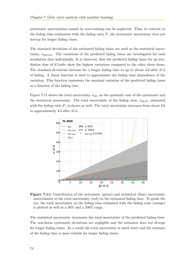
Chapter 7 Glow curve analysis with machine learning
systematic uncertainties caused by over-training can be neglected. Thus, in contrast to
the fading time estimation with the fading ratio F , the systematic uncertainty does not
diverge for longer fading times.
The standard deviations of the estimated fading times are used as the statistical uncer-
tainty, u∆t;stat. The variations of the predicted fading times are investigated for each
irradiation dose individually. It is observed, that the predicted fading times for an irra-
diation dose of 0.5 mSv show the highest variations compared to the other three doses.
The standard deviations increase for a longer fading time to up to about 4 d after 41 d
of fading. A linear function is used to approximate the fading time dependence of the
variation. This function represents the maximal variation of the predicted fading times
as a function of the fading time.
Figure 7.11 shows the total uncertainty, u∆t, as the quadratic sum of the systematic and
the statistical uncertainty. The total uncertainty of the fading time, u∆t;F , estimated
with the fading ratio F , is shown as well. The total uncertainty increases from about 8 h
to approximately 4 d after 41 d.
0 5 10 15 20 25 30 35 40t in d
0
10
20
30
40
50
60
u in
d
u t
u t; deviu t; statu t; F
± 50%± 100%u t; stat 0.5 mSv
TL-DOS
Figure 7.11: Contribution of the systematic (green) and statistical (blue) uncertaintyuncertainties to the total uncertainty (red) on the estimated fading time. To guide theeye, the total uncertainty on the fading time estimated with the fading ratio (orange)is plotted as well as a 50% and a 100% range.
The statistical uncertainty dominates the total uncertainty of the predicted fading time.
The non-linear systematic deviations are negligible and the estimator does not diverge
for longer fading times. As a result the total uncertainty is much lower and the estimate
of the fading time is more reliable for longer fading times.
74
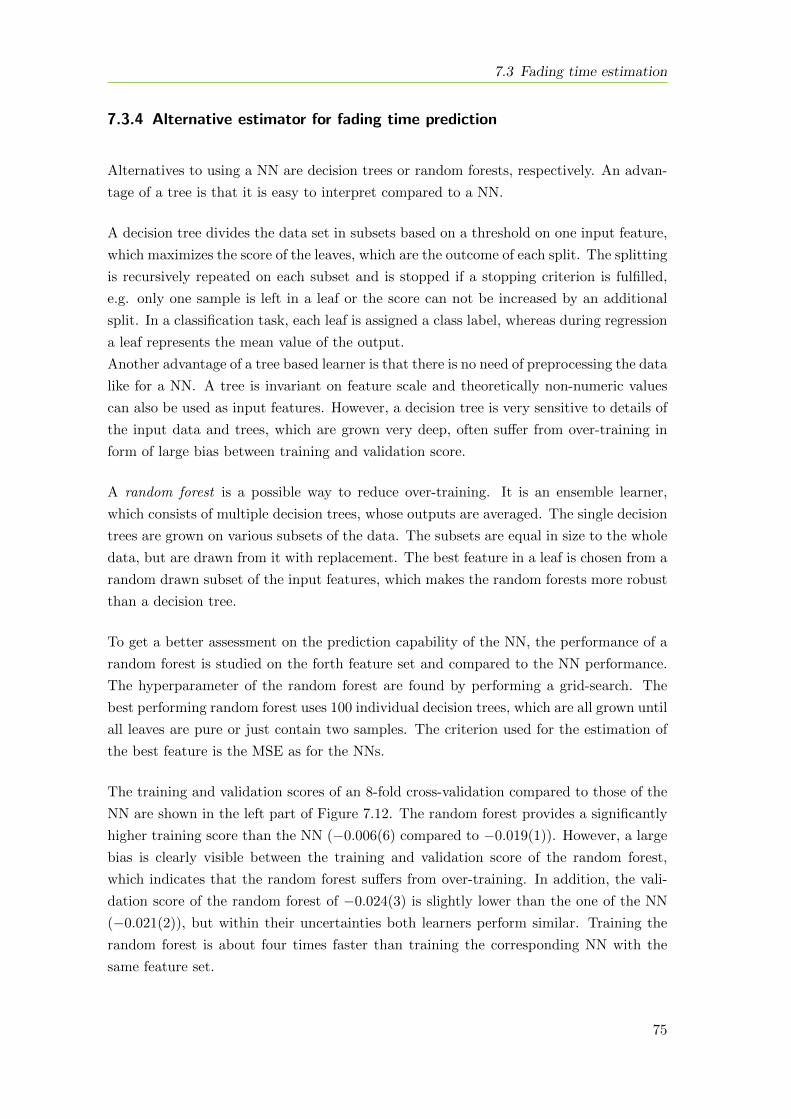
7.3 Fading time estimation
7.3.4 Alternative estimator for fading time prediction
Alternatives to using a NN are decision trees or random forests, respectively. An advan-
tage of a tree is that it is easy to interpret compared to a NN.
A decision tree divides the data set in subsets based on a threshold on one input feature,
which maximizes the score of the leaves, which are the outcome of each split. The splitting
is recursively repeated on each subset and is stopped if a stopping criterion is fulfilled,
e.g. only one sample is left in a leaf or the score can not be increased by an additional
split. In a classification task, each leaf is assigned a class label, whereas during regression
a leaf represents the mean value of the output.
Another advantage of a tree based learner is that there is no need of preprocessing the data
like for a NN. A tree is invariant on feature scale and theoretically non-numeric values
can also be used as input features. However, a decision tree is very sensitive to details of
the input data and trees, which are grown very deep, often suffer from over-training in
form of large bias between training and validation score.
A random forest is a possible way to reduce over-training. It is an ensemble learner,
which consists of multiple decision trees, whose outputs are averaged. The single decision
trees are grown on various subsets of the data. The subsets are equal in size to the whole
data, but are drawn from it with replacement. The best feature in a leaf is chosen from a
random drawn subset of the input features, which makes the random forests more robust
than a decision tree.
To get a better assessment on the prediction capability of the NN, the performance of a
random forest is studied on the forth feature set and compared to the NN performance.
The hyperparameter of the random forest are found by performing a grid-search. The
best performing random forest uses 100 individual decision trees, which are all grown until
all leaves are pure or just contain two samples. The criterion used for the estimation of
the best feature is the MSE as for the NNs.
The training and validation scores of an 8-fold cross-validation compared to those of the
NN are shown in the left part of Figure 7.12. The random forest provides a significantly
higher training score than the NN (−0.006(6) compared to −0.019(1)). However, a large
bias is clearly visible between the training and validation score of the random forest,
which indicates that the random forest suffers from over-training. In addition, the vali-
dation score of the random forest of −0.024(3) is slightly lower than the one of the NN
(−0.021(2)), but within their uncertainties both learners perform similar. Training the
random forest is about four times faster than training the corresponding NN with the
same feature set.
75
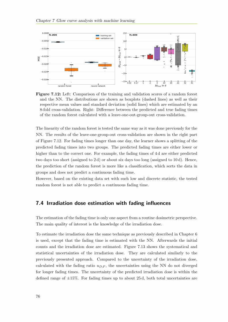
Chapter 7 Glow curve analysis with machine learning
random forest neural network
0.030
0.025
0.020
0.015
0.010
0.005
0.000
MSE
training setvalidation set
TL-DOS
0.02 0.17 1 2 4 10 16 22 32 41ttrue in d
15
10
5
0
5
10
15
t pre
dt tr
ue in
d
TL-DOS
Figure 7.12: Left: Comparison of the training and validation scores of a random forestand the NN. The distributions are shown as boxplots (dashed lines) as well as theirrespective mean values and standard deviation (solid lines) which are estimated by an8-fold cross-validation. Right: Difference between the predicted and true fading timesof the random forest calculated with a leave-one-out-group-out cross-validation.
The linearity of the random forest is tested the same way as it was done previously for the
NN. The results of the leave-one-group-out cross-validation are shown in the right part
of Figure 7.12. For fading times longer than one day, the learner shows a splitting of the
predicted fading times into two groups. The predicted fading times are either lower or
higher than to the correct one. For example, the fading times of 4 d are either predicted
two days too short (assigned to 2 d) or about six days too long (assigned to 10 d). Hence,
the prediction of the random forest is more like a classification, which sorts the data in
groups and does not predict a continuous fading time.
However, based on the existing data set with such low and discrete statistic, the tested
random forest is not able to predict a continuous fading time.
7.4 Irradiation dose estimation with fading influences
The estimation of the fading time is only one aspect from a routine dosimetric perspective.
The main quality of interest is the knowledge of the irradiation dose.
To estimate the irradiation dose the same technique as previously described in Chapter 6
is used, except that the fading time is estimated with the NN. Afterwards the initial
counts and the irradiation dose are estimated. Figure 7.13 shows the systematical and
statistical uncertainties of the irradiation dose. They are calculated similarly to the
previously presented approach. Compared to the uncertainty of the irradiation dose,
calculated with the fading ratio uD;F , the uncertainties using the NN do not diverged
for longer fading times. The uncertainty of the predicted irradiation dose is within the
defined range of ±15%. For fading times up to about 25 d, both total uncertainties are
76
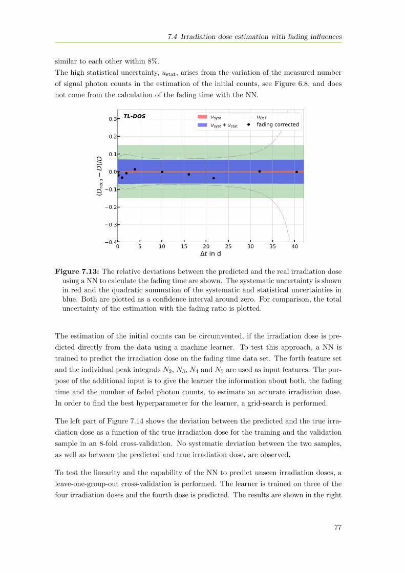
7.4 Irradiation dose estimation with fading influences
similar to each other within 8%.
The high statistical uncertainty, ustat, arises from the variation of the measured number
of signal photon counts in the estimation of the initial counts, see Figure 6.8, and does
not come from the calculation of the fading time with the NN.
0 5 10 15 20 25 30 35 40t in d
0.4
0.3
0.2
0.1
0.0
0.1
0.2
0.3
(Dre
coD
)/D
usystusyst + ustat
uD; Ffading corrected
TL-DOS
Figure 7.13: The relative deviations between the predicted and the real irradiation doseusing a NN to calculate the fading time are shown. The systematic uncertainty is shownin red and the quadratic summation of the systematic and statistical uncertainties inblue. Both are plotted as a confidence interval around zero. For comparison, the totaluncertainty of the estimation with the fading ratio is plotted.
The estimation of the initial counts can be circumvented, if the irradiation dose is pre-
dicted directly from the data using a machine learner. To test this approach, a NN is
trained to predict the irradiation dose on the fading time data set. The forth feature set
and the individual peak integrals N2, N3, N4 and N5 are used as input features. The pur-
pose of the additional input is to give the learner the information about both, the fading
time and the number of faded photon counts, to estimate an accurate irradiation dose.
In order to find the best hyperparameter for the learner, a grid-search is performed.
The left part of Figure 7.14 shows the deviation between the predicted and the true irra-
diation dose as a function of the true irradiation dose for the training and the validation
sample in an 8-fold cross-validation. No systematic deviation between the two samples,
as well as between the predicted and true irradiation dose, are observed.
To test the linearity and the capability of the NN to predict unseen irradiation doses, a
leave-one-group-out cross-validation is performed. The learner is trained on three of the
four irradiation doses and the fourth dose is predicted. The results are shown in the right
77
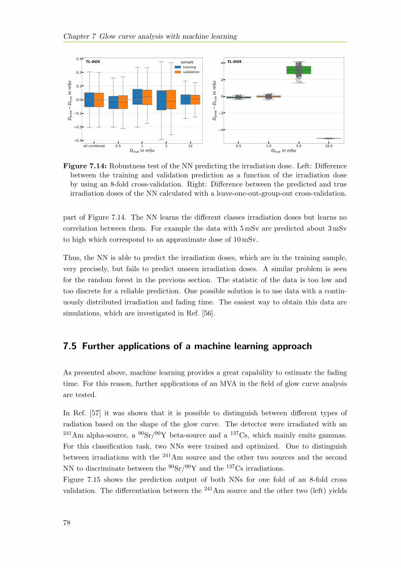
Chapter 7 Glow curve analysis with machine learning
all combined 0.5 1 5 10Dtrue in mSv
0.3
0.2
0.1
0.0
0.1
0.2
0.3
Dpr
edD
true i
n m
Svsample
trainingvalidation
TL-DOS
0.5 1.0 5.0 10.0Dtrue in mSv
4
2
0
2
4
Dpr
edD
true i
n m
Sv
TL-DOS
Figure 7.14: Robustness test of the NN predicting the irradiation dose. Left: Differencebetween the training and validation prediction as a function of the irradiation doseby using an 8-fold cross-validation. Right: Difference between the predicted and trueirradiation doses of the NN calculated with a leave-one-out-group-out cross-validation.
part of Figure 7.14. The NN learns the different classes irradiation doses but learns no
correlation between them. For example the data with 5 mSv are predicted about 3 mSv
to high which correspond to an approximate dose of 10 mSv.
Thus, the NN is able to predict the irradiation doses, which are in the training sample,
very precisely, but fails to predict unseen irradiation doses. A similar problem is seen
for the random forest in the previous section. The statistic of the data is too low and
too discrete for a reliable prediction. One possible solution is to use data with a contin-
uously distributed irradiation and fading time. The easiest way to obtain this data are
simulations, which are investigated in Ref. [56].
7.5 Further applications of a machine learning approach
As presented above, machine learning provides a great capability to estimate the fading
time. For this reason, further applications of an MVA in the field of glow curve analysis
are tested.
In Ref. [57] it was shown that it is possible to distinguish between different types of
radiation based on the shape of the glow curve. The detector were irradiated with an241Am alpha-source, a 90Sr/90Y beta-source and a 137Cs, which mainly emits gammas.
For this classification task, two NNs were trained and optimized. One to distinguish
between irradiations with the 241Am source and the other two sources and the second
NN to discriminate between the 90Sr/90Y and the 137Cs irradiations.
Figure 7.15 shows the prediction output of both NNs for one fold of an 8-fold cross
validation. The differentiation between the 241Am source and the other two (left) yields
78
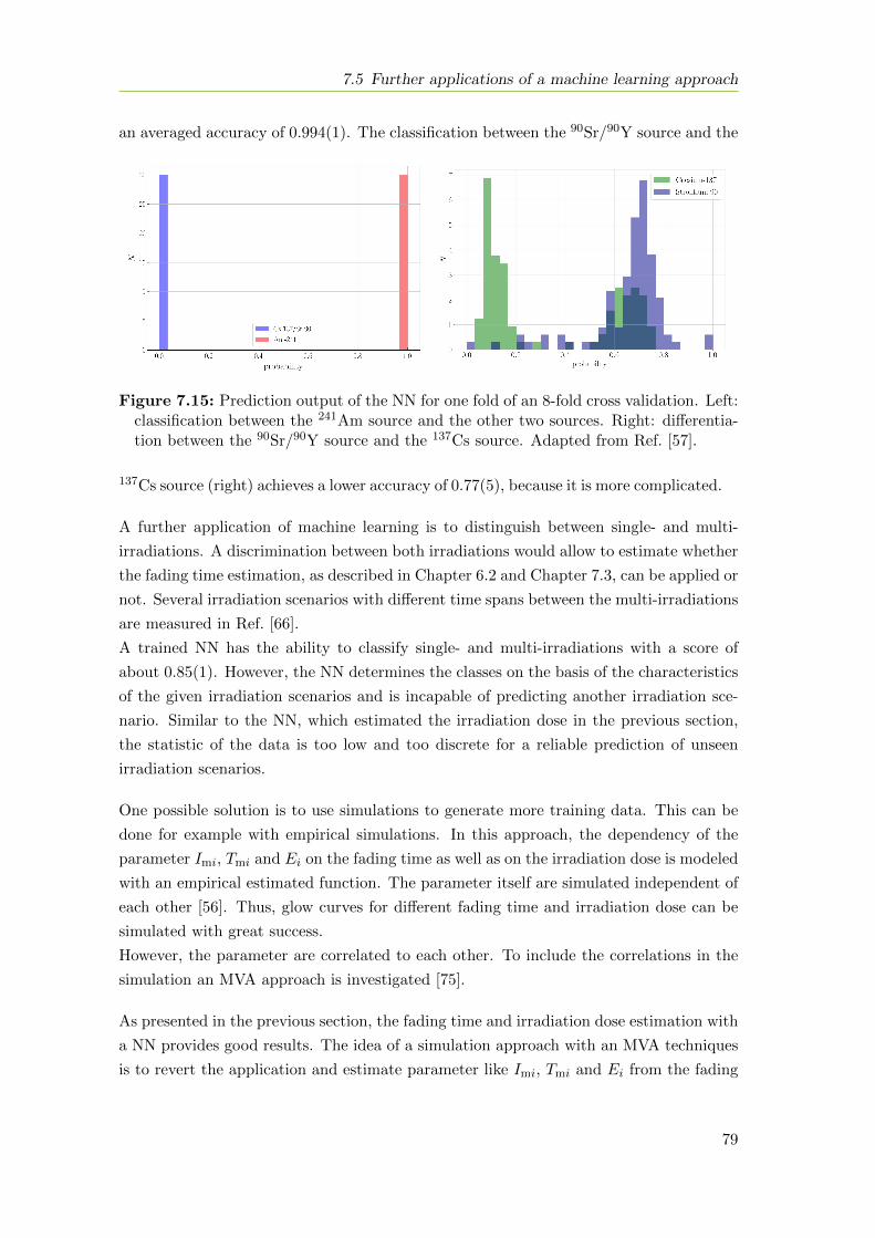
7.5 Further applications of a machine learning approach
an averaged accuracy of 0.994(1). The classification between the 90Sr/90Y source and the
Figure 7.15: Prediction output of the NN for one fold of an 8-fold cross validation. Left:classification between the 241Am source and the other two sources. Right: differentia-tion between the 90Sr/90Y source and the 137Cs source. Adapted from Ref. [57].
137Cs source (right) achieves a lower accuracy of 0.77(5), because it is more complicated.
A further application of machine learning is to distinguish between single- and multi-
irradiations. A discrimination between both irradiations would allow to estimate whether
the fading time estimation, as described in Chapter 6.2 and Chapter 7.3, can be applied or
not. Several irradiation scenarios with different time spans between the multi-irradiations
are measured in Ref. [66].
A trained NN has the ability to classify single- and multi-irradiations with a score of
about 0.85(1). However, the NN determines the classes on the basis of the characteristics
of the given irradiation scenarios and is incapable of predicting another irradiation sce-
nario. Similar to the NN, which estimated the irradiation dose in the previous section,
the statistic of the data is too low and too discrete for a reliable prediction of unseen
irradiation scenarios.
One possible solution is to use simulations to generate more training data. This can be
done for example with empirical simulations. In this approach, the dependency of the
parameter Imi, Tmi and Ei on the fading time as well as on the irradiation dose is modeled
with an empirical estimated function. The parameter itself are simulated independent of
each other [56]. Thus, glow curves for different fading time and irradiation dose can be
simulated with great success.
However, the parameter are correlated to each other. To include the correlations in the
simulation an MVA approach is investigated [75].
As presented in the previous section, the fading time and irradiation dose estimation with
a NN provides good results. The idea of a simulation approach with an MVA techniques
is to revert the application and estimate parameter like Imi, Tmi and Ei from the fading
79
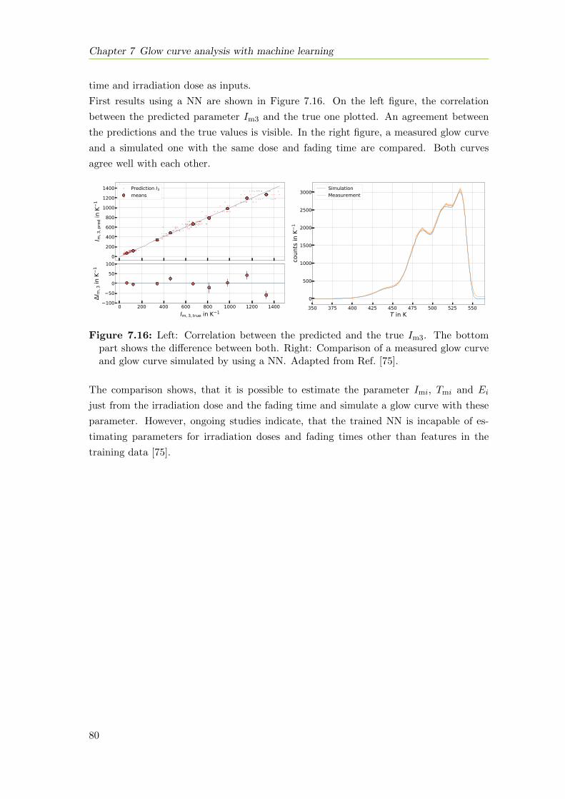
Chapter 7 Glow curve analysis with machine learning
time and irradiation dose as inputs.
First results using a NN are shown in Figure 7.16. On the left figure, the correlation
between the predicted parameter Im3 and the true one plotted. An agreement between
the predictions and the true values is visible. In the right figure, a measured glow curve
and a simulated one with the same dose and fading time are compared. Both curves
agree well with each other.
0200400600800
100012001400
I m,3
,pre
din
K1
Prediction I3means
0 200 400 600 800 1000 1200 1400Im, 3, true in K 1
10050
050
100
I m,3
inK
1
350 375 400 425 450 475 500 525 550T in K
0
500
1000
1500
2000
2500
3000
coun
ts in
K1
SimulationMeasurement
Figure 7.16: Left: Correlation between the predicted and the true Im3. The bottompart shows the difference between both. Right: Comparison of a measured glow curveand glow curve simulated by using a NN. Adapted from Ref. [75].
The comparison shows, that it is possible to estimate the parameter Imi, Tmi and Ei
just from the irradiation dose and the fading time and simulate a glow curve with these
parameter. However, ongoing studies indicate, that the trained NN is incapable of es-
timating parameters for irradiation doses and fading times other than features in the
training data [75].
80
Chapter 8
Summary and outlook
As shown it is possible to estimate the irradiation dose independent of the fading time
as well as the fading time itself directly from the glow curve. Two different approaches
were presented, one based on just one variable and one based on multiple variables.
The fading ratio allows for a robust estimation of the fading time independent of the
irradiation dose and energy. The uncertainty on the fading time is about 50% for fading
times between 5 d and 25 d and less than 100% for fading times up to 34 d. For longer
fading times the systematical uncertainty increases dramatically and no reliable estima-
tion of the fading ratio can be made.
When the fading time is known the measured signal photon counts are corrected and a
fading time independent irradiation dose is estimated with an uncertainty in the given
range of ±15% for fading times lower than 34 d, which is a common time interval in
individual routine dose monitoring.
The uncertainties of the fading time estimation with the univariate analysis were sig-
nificantly lowered by using a machine learning approach. A neural network (NN) was
trained to estimate the fading time from multiple input features. The performance of NN
using different feature sets was investigated and a subset of all features was identified,
which optimizes the overall performance. The systematic uncertainty of the predicted
fading time does not diverge for longer fading times and the total uncertainty is reduced
to approximately 4 d for a fading time of 41 d. A comparison between two different types
of machine learning algorithms showed that a NN performs better than a random forest
on the data set which has a discrete distribution and low statistics.
To estimate the irradiation dose two approaches were studied. In the first approach the
predicted fading time of the NN is used to correct the measured signal photon counts and
estimate a fading time independent irradiation dose. Compared to the irradiation dose
estimation using the univariate method, the total uncertainty on the irradiation dose is
dominated by the statistical uncertainty and does not increase for longer fading times.
81
Chapter 8 Summary and outlook
The irradiation dose can be predicted with an uncertainty of about 8% for fading times
up to 41 d.
The second approach uses a NN to directly estimate the irradiation. However, due to low
and very discrete statistic the learner is not able to predict unseen irradiation doses reli-
able. By using continuously distributed simulated data, the estimation of the irradiation
dose with a NN can be improved.
The glow curves are recorded as a function of time and due to sensitivity issues the reader
is not able to measure the temperature. However, both the uni- and the multivariate
obtain information from the glow curve as a function of the temperature. Therefore,
a method was developed to transform glow curves from the time into the temperature
domain even without measuring the temperature. By estimating the peak positions in
the time domain, the individual heating profile is reconstructed and the glow curve is
transformed from time into temperature space.
Using the measured data, several detector and reader characteristics were studied result-
ing in a better understanding of the TL-DOS dosemeters. It was confirmed that the
reflective layer has no visible effect on the measured TL signal and thus can be omitted.
Furthermore, it has been shown that detectors from a later batch have a smaller variation
in their response.
A significant decrease of the PMT’s sensitivity over time was observed during the mea-
surements. Although the reason for this loss is unknown, the data can be corrected due
to reference measurements performed between them.
By using information of the individual glow peaks, the fading time of a dosemeter is
estimated directly from the glow curve. With the known fading time, the estimation of
the irradiation dose of TL dosemeters in the TL-DOS project is significantly improved.
The results of this thesis can be applied in the field of routine dosimetry to improve the
analysis.
82

Acronyms
EURADOS European Radiation Dosimetry Group
GCD glow curve deconvolution
Hp(0.07) skin dose
Hp(3) eye lens dose
Hp(10) whole body dose
ICRP International Commission on Radiological Protection
IQR inter quartile range
LiF:Mg,Ti Lithium Fluorine doped with Magnesium and Titanium
MLP multi-layer perceptron
MPA NRW Materialprufungsamt North Rhine-Westphalia
MSE mean squared error
MVA multivariate analysis
NN neural network
OSL optically stimulated luminescence
OTOR one trap one recombination center
PCA principal component analysis
PMT photo multiplier tube
PTB Physikalisch-Technische Bundesanstalt
PTFE polytetrafluoroethylene
RoeV ”Rontgenverordnung”, X-ray Protection Ordinance
RoI region of interest
StrlSchV ”Strahlenschutzverordnung”, Radiation Protection Ordinance
TL thermoluminescence
TL-DOS thermoluminescence dosemeter system
83

84
Bibliography
[1] R. Boyle. Register of the Royal Society, 1663:213, 1663.
[2] J. T. Randall and M. H. F. Wilkins. Phosphorescence and Electron Traps. I. TheStudy of Trap Distributions. Proceedings of the Royal Society of London A: Mathe-matical, Physical and Engineering Sciences, 184(999):365–389, 1945.
[3] R. Theinert et al. Computational analysis of thermoluminescence glow curves fromthin layer dosemeters. Radiation Measurements, 106:252–256, 2017. Proceedingsof the 18th International Conference on Solid State Dosimetry (SSD18), Munich,Germany, 3 – 8 July 2016.
[4] R. Theinert et al. Fading time and irradiation dose estimation from thermolumines-cent dosemeters using glow curve deconvolution. Radiation Measurements, 108:20–25, 2018.
[5] Verordnung uber den Schutz vor Schaden durch ionisierende Strahlen (Strahlen-schutzverordnung - StrlSchV) , 2001. Last changed according to para. 10 persuantto para. 6 G v. 27.1.2017 I 114, 1222.
[6] Verordnung uber den Schutz vor Schaden durch Rontgenstrahlen (Rontgenverord-nung - RoV) . 2003. Last changed pursuant to para. 6 V v. 11.12.2014 I 2010.
[7] The 2007 Recommendations of the International Commission on Radiological Pro-tection. Annals of the ICRP, 37(2-4), 2007. ICRP Publication 103.
[8] Physikalisch-Technische Bundesanstalt. PTB-Anforderungen PTB-A 23.2 ”Strahlen-schutzmessgerate; Personendosimeter zur Messung der Tiefen- und Oberflachen-Personendosis”, November 2013.
[9] IEC 62387: Radiation protection instrumentation - Passive integrating dosimetrysystems for personal and environmental monitoring of photon and beta radiation,2007.
[10] K.-H. Ritzenhoff et al. A new film badge for the measurement of the personaldose equivalent Hp(10) using the gliding-shadow method. In Proceedings of the 9.International Congress on Radiation Protection, Wien 1996, volume 4, pages 266–268. 1996.
[11] G. F. J. Garlick and A. F. Gibson. The Electron Trap Mechanism of Luminescencein Sulphide and Silicate Phosphors. Proceedings of the Physical Society, 60(6):574,1948.
[12] C. E. May and J. A. Partridge. Thermoluminescent Kinetics of Alpha-IrradiatedAlkali Halides. The Journal of Chemical Physics, 40(5):1401–1409, 1964.
85
Bibliography
[13] V. Pagonis, G. Kitis and C. Furetta. Numerical and Practical Exercises in Thermo-luminescence. Springer-Verlag New York, 1 edition, 2006.
[14] R. Chen and V. Pagonis. Thermally and Optically Stimulated Luminescence: ASimulation Approach. John Wiley & Sons, Ltd, 2011.
[15] C. M. Sunta. Unraveling Thermoluminescence. Springer India, 1 edition, 2015.
[16] Y. S. Horowitz and M. Moscovitch. Highlights and pitfalls of 20 years of applicationof computerised glow curve analysis to thermoluminescence research and dosimetry.Radiation Protection Dosimetry, 153(1):1–22, 2013.
[17] Y. Horowitz. Thermoluminescence dosimetry: State-of-the-art and frontiers of futureresearch. Radiation Measurements, 71:2–7, 2014. Proceedings of the 17th Solid StateDosimetry Conference (SSD17).
[18] J. A. Harvey, N. P. Haverland and K. J. Kearfott. Characterization of the glow-peakfading properties of six common thermoluminescent materials. Applied Radiationand Isotopes, 68(10):1988–2000, 2010.
[19] Radcard - TLD Dosemeters. URL http://www.radcard.pl/index.html, [Online;accessed 2018-06-04].
[20] B. Marczewska et al. Imaging of proton bragg peaks in LiF. Radiation ProtectionDosimetry, 178(3):333–336, 2018.
[21] P. Bilski et al. Lithium fluoride cryatals as fluorescent nuclear track detectors. Ra-diation Protection Dosimetry, 178(3):337–340, 2018.
[22] J. Walbersloh and F. Busch. A thin-layer LiF thermoluminescence dosemeter systemwith fast readout for the use in personal dosimetry services. Radiation ProtectionDosimetry, 170(1-4):191–194, 2016.
[23] Y. Lee, Y. Won and K. Kang. A method to minimise the fading effects of LiF:Mg,Ti(TLD-600 and TLD-700) using a pre-heat technique. Radiation Protection Dosime-try, 164(3):449–455, 2015.
[24] M. Piepenbrock. Entwicklung einert Dosimetersonde zur Bestimmung der Tiefenper-sonendosis Hp(10) und der Oberflachendosis Hp(0.07) mit dem Thermolumineszenz-Dunnschichtdosimeter-System TL-DOS. Master’s thesis, TU Dortmund, 2016.
[25] M. Piepenbrock et al. Development of a badge for the thin-layer thermoluminescencedosemeter system TL-DOS to measure the personal dose equivalent Hp(10) andHp(0.07). Radiation Measurements, 106:543–545, 2017. Proceedings of the 18thInternational Conference on Solid State Dosimetry (SSD18), Munich, Germany, 3 –8 July 2016.
[26] W. Hantke. Labortests zur Uberprufung des routinemaßigen Einsatzes von TL-DOSGanzkorperdosimetern. Master’s thesis, TU Dortmund, 2018.
[27] M. Heiny. Design und Prototypen-Entwicklung eines Fingerringdosimeters zur Bes-timmung der Teilkorperpersonendosis Hp(0.07). Master’s thesis, TU Dortmund,2016.
86

Bibliography
[28] K. Honer. Untersuchung geometrischer Einflussfaktoren auf das Ansprechvermogeneines Beta-Fingerringdosimeters bei Bestrahlungen mit einem Beta-Sekundarnormal.Master’s thesis, TU Dortmund, 2017.
[29] M. Schidlowski. Entwicklung, Charakterisierung und klinische Erprobung einesHp(3)-TL-Augenlinsendosimeters. Master’s thesis, TU Dortmund, 2017.
[30] C.-M. Linker. Feldkalibrierung eines Albedo-Neutronendosimeters in einem Proto-nentherapiezentrum. Master’s thesis, TU Dortmund, 2017.
[31] M. Heiny. Ph.D. thesis, TU Dortmund. Dissertation in preparation.
[32] L. Fecke. Hochdosisverhalten von Thermolumineszenz-Dunnschichtdetektoren. Bach-elor’s thesis, Heinrich Heine Universitat Dusseldorf, 2015.
[33] W. Gieszczyk and P. Bilski. A simplified numerical approach to non-radiation in-duced high-temperature signals in thermoluminescence. GlowVIEW – a useful toolfor a multiple glow-curve analysis. Radiation Measurements, 107:102–110, 2017.
[34] A. J. J. Bos et al. Effects of cooling and heating rate on trapping parameters inLiF:Mg, Ti crystals. Journal of Physics D: Applied Physics, 25(8):1249–1257, 1992.
[35] S. Mender. Bestimmung der Nachweisgrenze des Thermolumineszenzdosimetersys-tems TL-DOS fur die Tiefenpersonendosis Hp(10). Bachelor’s thesis, TU Dortmund,2016.
[36] E. Jones, T. Oliphant, P. Peterson et al. SciPy: Open source scientific tools forPython, 2001. URL http://www.scipy.org, [Online; accessed 2017-07-27].
[37] W. McKinney. Data Structures for Statistical Computing in Python. In S. van derWalt and J. Millman, editors, Proceedings of the 9th Python in Science Conference,pages 51–56. 2010.
[38] F. Pedregosa et al. Scikit-learn: Machine Learning in Python. Journal of MachineLearning Research, 12:2825–2830, 2011.
[39] J. D. Hunter. Matplotlib: A 2D Graphics Environment. Computing in Science &Engineering, 9(3):90–95, June 2007.
[40] M. Waskom et al. seaborn: v0.8.1, September 2017.
[41] J. van Dijk and H. Julius. Glow Curve Analysis for Constant Temperature Hot GasTLD Readers. Radiation Protection Dosimetry, 47(1-4):479–482, 1993.
[42] J. van Dijk and F. Busscher. The Zero Signal and Glow Curves of Bare LiF:Mg,TiDetectors in a Hot Gas TLD System. Radiation Protection Dosimetry, 101(1-4):59–64, 2002.
[43] H. Stadtmann, C. Hranitzky and N. Brasik. Study of real time temperature profilesin routine TLD read out—influences of detector thickness and heating rate on glowcurve shape. Radiation Protection Dosimetry, 119(1-4):310–313, 2006.
[44] A. Savitzky and M. J. E. Golay. Smoothing and Differentiation of Data by SimplifiedLeast Squares Procedures. Analytical Chemistry, 36(8):1627–1639, 1964.
87
Bibliography
[45] A. Lutfring. Charakterisierung des Aufheitsverhaltens und gluhkurvenbasierte Rekon-struktion der Detektortemperatur eines Dunnschicht-Thermolumineszenzdosimeters.Master’s thesis, TU Dortmund, 2016.
[46] G. Kitis, J. M. Gomez-Ros and J. W. N. Tuyn. Thermoluminescence glow-curvedeconvolution functions for first, second and general orders of kinetics. Journal ofPhysics D: Applied Physics, 31(19):2636–2641, 1998.
[47] A. Bos et al. An Intercomparison of Glow Curve Analysis Computer Programs: I.Synthetic Glow Curves. Radiation Protection Dosimetry, 47(1-4):473–477, 1993.
[48] A. Bos et al. An Intercomparison of Glow Curve Analysis Computer Programs: II.Measured Glow Curves. Radiation Protection Dosimetry, 51(4):257–264, 1994.
[49] V. Pagonis, S. Mian and G. Kitis. Fit of First Order Thermoluminescence GlowPeaks using the Weibull Distribution Function. Radiation Protection Dosimetry,93(1):11–17, 2001.
[50] V. Pagonis and G. Kitis. Fit of Second Order Thermoluminescence Glow Peaks Usingthe Logistic Distribution Function. Radiation Protection Dosimetry, 95(3):225–229,2001.
[51] G. Kitis et al. Thermoluminescence under an exponential heating function: I. The-ory. Journal of Physics D: Applied Physics, 39(8):1500–1507, 2006.
[52] G. Kitis et al. Thermoluminescence under an exponential heating function: II. Glow-curve deconvolution of experimental glow-curves. Journal of Physics D: AppliedPhysics, 39(8):1508–1514, 2006.
[53] M. Moscovitch, Y. Horowitz and J. Oduko. LiF Thermoluminescence Dosimetryvia Computerised First Order Kinetics Glow Curve Analysis. Radiation ProtectionDosimetry, 6(1-4):157–159, 1983.
[54] Y. Horowitz, M. Moscovitch and M. Wilt. Computerized glow curve deconvolutionapplied to ultralow dose LiF thermoluminescence dosimetry. Nuclear Instrumentsand Methods in Physics Research Section A: Accelerators, Spectrometers, Detectorsand Associated Equipment, 244(3):556–564, 1986.
[55] G. Kitis, E. Carinou and P. Askounis. Glow-curve de-convolution analysis of TL glow-curve from constant temperature hot gas TLD readers. Radiation Measurements,47(4):258–265, 2012.
[56] F. Mentzel. Master’s thesis, TU Dortmund, 2018. Thesis in preparation.
[57] M. Steil. Gluhkurvenanalyse zur Unterscheidung von Strahlungsarten mittels Multi-variaten Analysemethoden. Bachelor’s thesis, TU Dortmund, 2018.
[58] Y. Horowitz. Editorial - Fading in LiF:Mg,Ti. Radiation Protection Dosimetry,32(3):147, 1990.
[59] S. Doremus and G. Higgins. Pre-Irradiation Fade and Post-Irradiation Fade forLiF:Mg,Ti, TLD-600, and TLD-700, as a Function of Time. Radiation ProtectionDosimetry, 54(2):119–125, 1994.
88
Bibliography
[60] C. Furetta, C. Kuo and P. Weng. Fading prediction in thermoluminescent materialsusing computerised glow curve deconvolution (CGCD). Nuclear Instruments andMethods in Physics Research Section A: Accelerators, Spectrometers, Detectors andAssociated Equipment, 423(1):183–189, 1999.
[61] M. Weinstein et al. A simple method for avoiding fading correction of absorbed dosefrom glow curves of TLD-100. Radiation Measurements, 37(1):81–86, 2003.
[62] M. Moscovitch. Automatic Method for Evaluating Elapsed Time Between Irradiationand Readout in LiF-TLD. Radiation Protection Dosimetry, 17(1-4):165–169, 1986.
[63] C. Furetta and J. Azorın. Simultaneous determination of dose and time elapsed sinceirradiation using CaSO4:Dy thermoluminescent dosimeters. Nuclear Instruments andMethods in Physics Research Section A: Accelerators, Spectrometers, Detectors andAssociated Equipment, 280(2):318–321, 1989.
[64] M. Budzanowski et al. Estimation of the Time Elapsed Between Exposure andReadout Using Peak Ratios of LiF:Mg,Cu,P (MCP-N,GR200A). Radiation Protec-tion Dosimetry, 85(1-4):149–152, 1999.
[65] J. A. Harvey and K. J. Kearfott. Reproducibility of glow peak fading characteristicsof thermoluminescent dosimeters. Radiation Measurements, 46(3):319–322, 2011.
[66] J. Lingweiler. Vorstudie zur Unterscheidung von Einfach- und Mehrfachbestrahlungvon Thermolumineszenzdosimetern mithilfe von Multivariater Analyse. Bachelor’sthesis, TU Dortmund, 2018.
[67] L. Speicher. Untersuchung des Einflusses von Pre-Irradiation-Fading auf Gluhkur-ven. Bachelor’s thesis, TU Dortmund, 2018.
[68] C. Bishop. Pattern Recognition and Machine Learning. Information Science andStatistics. Springer, 2006.
[69] T. Hastie, R. Tibshirani and J. Friedman. The Elements of Statistical Learning:Data Mining, Inference, and Prediction, Second Edition. Springer Series in Statistics.Springer New York, 2 edition, 2009.
[70] M. Kubat. An Introduction to Machine Learning. Springer International Publishing,2 edition, 2017.
[71] F. Rosenblatt. The perceptron: A probabilistic model for information storage andorganization in the brain. Psychological Review, 65(6):386–408, 1958.
[72] K. Hornik, M. Stinchcombe and H. White. Multilayer feedforward networks areuniversal approximators. Neural Networks, 2(5):359–366, 1989.
[73] J. Nocedal. Updating Quasi-Newton Matrices with Limited Storage. Mathematicsof computation, 35:773–782, 07 1980.
[74] D. P. Kingma and J. Ba. Adam: A Method for Stochastic Optimization. CoRR,abs/1412.6980, 2014.
[75] L. Rohrig. Bachelor’s thesis, TU Dortmund, 2018. Thesis in preparation.
89

90

Danksagung
An dieser Stelle mochte ich mich bei allen bedanken, die mich wahrend meines Studiums
unterstutzt und mir geholfen haben, diese Arbeit anzufertigen.
Zuerst mochte ich Prof. Dr. Kevin Kroninger danken, der mir die Moglichkeit gegeben
hat, an seinem Lehrstuhl zu arbeiten und mich wahrend dieser Zeit betreut hat.
Des Weiteren mochte ich Prof. Dr. Dr. Wolfgang Rhode sowie allen Mitgliedern der
Prufungskommission meinen Dank aussprechen, dass sie sich bereit erklart haben, meine
Arbeit zu lesen und zu bewerten.
Zudem bin ich Jorg, HWK, Myriam und dem gesamten Team am MPA sehr verbunden,
dass sie mir wahrend der Durchfuhrung meiner Messungen mit Rat und Tat zur Seite
standen.
Fur die gute Zusammenarbeit, die schone Zeit am Lehrstuhl sowie die leckeren Kuchen
mochte ich mich bei allen aktuellen und ehemaligen Mitgliedern des Lehrstuhl EIV be-
danken und mochte dabei besonders die beiden guten Seelen des Lehrstuhls, Markus und
Andrea, hervorheben.
Mein Dank gilt auch Jens, Olaf und Flo die meine Arbeit kritisch gelesen haben und mir
mit dem ein oder anderen Kommentar geholfen haben, sie zu verbessern. Abschließend
mochte ich noch Flo besonders danken, der mir geholfen hat, die verschiedenen Fits und
Berechnungen in unsere Software zu implementieren, zu testen und zu dokumentieren.
Zu guter Letzt mochte ich besonders meiner Familie und meiner Freundin sagen:
Danke, dass ihr immer fur mich da seid.
91
Copyright © 2022 FDOKUMEN