
Stable Maximum Throughput Broadcast in Wireless Fading Channels
9
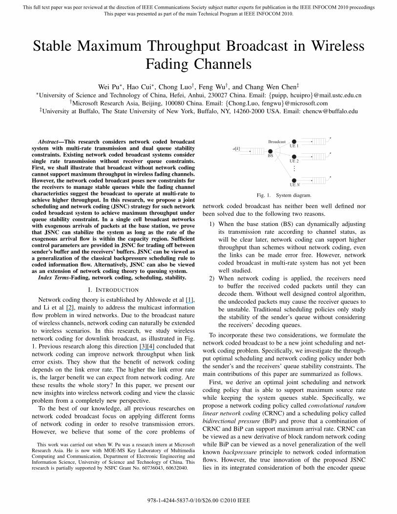
Stable Maximum Throughput Broadcast in Wireless Fading Channels Wei Pu ∗ , Hao Cui ∗ , Chong Luo † , Feng Wu † , and Chang Wen Chen ‡ ∗ University of Science and Technology of China, Hefei, Anhui, 230027 China. Email: {puipp, hcuipro}@mail.ustc.edu.cn † Microsoft Research Asia, Beijing, 100080 China. Email: {Chong.Luo, fengwu}@microsoft.com ‡ University at Buffalo, The State University of New York, Buffalo, NY, 14260-2000 USA. Email: [email protected] Abstract—This research considers network coded broadcast system with multi-rate transmission and dual queue stability constraints. Existing network coded broadcast systems consider single rate transmission without receiver queue constraints. First, we shall illustrate that broadcast without network coding cannot support maximum throughput in wireless fading channels. However, the network coded broadcast poses new constraints for the receivers to manage stable queues while the fading channel characteristics suggest the broadcast to operate at multi-rate to achieve higher throughput. In this research, we propose a joint scheduling and network coding (JSNC) strategy for such network coded broadcast system to achieve maximum throughput under queue stability constraint. In a single cell broadcast networks with exogenous arrivals of packets at the base station, we prove that JSNC can stabilize the system as long as the rate of the exogenous arrival flow is within the capacity region. Sufficient control parameters are provided in JSNC for trading off between sender’s buffer and the receivers’ buffers. JSNC can be viewed as a generalization of the classical backpressure scheduling rule to coded information flow. Alternatively, JSNC can also be viewed as an extension of network coding theory to queuing system. Index Terms-Fading, network coding, scheduling, stability. I. I NTRODUCTION Network coding theory is established by Ahlswede et al [1], and Li et al [2], mainly to address the multicast information flow problem in wired networks. Due to the broadcast nature of wireless channels, network coding can naturally be extended to wireless scenarios. In this research, we study wireless network coding for downlink broadcast, as illustrated in Fig. 1. Previous research along this direction [3][4] concluded that network coding can improve network throughput when link error exists. They show that the benefit of network coding depends on the link error rate. The higher the link error rate is, the larger benefit we can expect from network coding. Are these results the whole story? In this paper, we present our new insights into wireless network coding and view the classic problem from a completely new perspective. To the best of our knowledge, all previous researches on network coded broadcast focus on applying different forms of network coding in order to resolve transmission errors. However, we believe that some of the core problems of This work was carried out when W. Pu was a research intern at Microsoft Research Asia. He is now with MOE-MS Key Laboratory of Multimedia Computing and Communication, Department of Electronic Engineering and Information Science, University of Science and Technology of China. This research is partially supported by NSFC Grant No. 60736043, 60632040. Broadcast BS UE N UE 2 UE 1 # a[k] Fig. 1. System diagram. network coded broadcast has neither been well defined nor been solved due to the following two reasons. 1) When the base station (BS) can dynamically adjusting its transmission rate according to channel status, as will be clear later, network coding can support higher throughput than schemes without network coding, even the links can be made error free. However, network coded broadcast in multi-rate system has not yet been well studied. 2) When network coding is applied, the receivers need to buffer the received coded packets until they can decode them. Without well designed control algorithm, the undecoded packets may cause the receiver queues to be unstable. Traditional scheduling policies only study the stability of the sender’s queue without considering the receivers’ decoding queues. To incorporate these two considerations, we formulate the network coded broadcast to be a new joint scheduling and net- work coding problem. Specifically, we investigate the through- put optimal scheduling and network coding policy under both the sender’s and the receivers’ queue stability constraints. The main contributions of this paper are summarized as follows. First, we derive an optimal joint scheduling and network coding policy that is able to support maximum source rate while keeping the system queues stable. Specifically, we propose a network coding policy called convolutional random linear network coding (CRNC) and a scheduling policy called bidirectional pressure (BiP) and prove that a combination of CRNC and BiP can support maximum arrival rate. CRNC can be viewed as a new derivative of block random network coding while BiP can be viewed as a novel generalization of the well known backpressure principle to network coded information flows. However, the true innovation of the proposed JSNC lies in its integrated consideration of both the encoder queue 978-1-4244-5837-0/10/$26.00 ©2010 IEEE This full text paper was peer reviewed at the direction of IEEE Communications Society subject matter experts for publication in the IEEE INFOCOM 2010 proceedings This paper was presented as part of the main Technical Program at IEEE INFOCOM 2010.
-
Upload
independent -
Category
Documents
-
view
0 -
download
0
Transcript of Stable Maximum Throughput Broadcast in Wireless Fading Channels
Stable Maximum Throughput Broadcast in WirelessFading Channels
Wei Pu∗, Hao Cui∗, Chong Luo†, Feng Wu†, and Chang Wen Chen‡∗University of Science and Technology of China, Hefei, Anhui, 230027 China. Email: {puipp, hcuipro}@mail.ustc.edu.cn
†Microsoft Research Asia, Beijing, 100080 China. Email: {Chong.Luo, fengwu}@microsoft.com‡University at Buffalo, The State University of New York, Buffalo, NY, 14260-2000 USA. Email: [email protected]
Abstract—This research considers network coded broadcastsystem with multi-rate transmission and dual queue stabilityconstraints. Existing network coded broadcast systems considersingle rate transmission without receiver queue constraints.First, we shall illustrate that broadcast without network codingcannot support maximum throughput in wireless fading channels.However, the network coded broadcast poses new constraints forthe receivers to manage stable queues while the fading channelcharacteristics suggest the broadcast to operate at multi-rate toachieve higher throughput. In this research, we propose a jointscheduling and network coding (JSNC) strategy for such networkcoded broadcast system to achieve maximum throughput underqueue stability constraint. In a single cell broadcast networkswith exogenous arrivals of packets at the base station, we provethat JSNC can stabilize the system as long as the rate of theexogenous arrival flow is within the capacity region. Sufficientcontrol parameters are provided in JSNC for trading off betweensender’s buffer and the receivers’ buffers. JSNC can be viewed asa generalization of the classical backpressure scheduling rule tocoded information flow. Alternatively, JSNC can also be viewedas an extension of network coding theory to queuing system.
Index Terms-Fading, network coding, scheduling, stability.
I. INTRODUCTION
Network coding theory is established by Ahlswede et al [1],and Li et al [2], mainly to address the multicast informationflow problem in wired networks. Due to the broadcast natureof wireless channels, network coding can naturally be extendedto wireless scenarios. In this research, we study wirelessnetwork coding for downlink broadcast, as illustrated in Fig.1. Previous research along this direction [3][4] concluded thatnetwork coding can improve network throughput when linkerror exists. They show that the benefit of network codingdepends on the link error rate. The higher the link error rateis, the larger benefit we can expect from network coding. Arethese results the whole story? In this paper, we present ournew insights into wireless network coding and view the classicproblem from a completely new perspective.
To the best of our knowledge, all previous researches onnetwork coded broadcast focus on applying different formsof network coding in order to resolve transmission errors.However, we believe that some of the core problems of
This work was carried out when W. Pu was a research intern at MicrosoftResearch Asia. He is now with MOE-MS Key Laboratory of MultimediaComputing and Communication, Department of Electronic Engineering andInformation Science, University of Science and Technology of China. Thisresearch is partially supported by NSFC Grant No. 60736043, 60632040.
Broadcast
BS
UE N
UE 2
UE 1a[k]
Fig. 1. System diagram.
network coded broadcast has neither been well defined norbeen solved due to the following two reasons.
1) When the base station (BS) can dynamically adjustingits transmission rate according to channel status, aswill be clear later, network coding can support higherthroughput than schemes without network coding, eventhe links can be made error free. However, networkcoded broadcast in multi-rate system has not yet beenwell studied.
2) When network coding is applied, the receivers needto buffer the received coded packets until they candecode them. Without well designed control algorithm,the undecoded packets may cause the receiver queues tobe unstable. Traditional scheduling policies only studythe stability of the sender’s queue without consideringthe receivers’ decoding queues.
To incorporate these two considerations, we formulate thenetwork coded broadcast to be a new joint scheduling and net-work coding problem. Specifically, we investigate the through-put optimal scheduling and network coding policy under boththe sender’s and the receivers’ queue stability constraints. Themain contributions of this paper are summarized as follows.
First, we derive an optimal joint scheduling and networkcoding policy that is able to support maximum source ratewhile keeping the system queues stable. Specifically, wepropose a network coding policy called convolutional randomlinear network coding (CRNC) and a scheduling policy calledbidirectional pressure (BiP) and prove that a combination ofCRNC and BiP can support maximum arrival rate. CRNC canbe viewed as a new derivative of block random network codingwhile BiP can be viewed as a novel generalization of the wellknown backpressure principle to network coded informationflows. However, the true innovation of the proposed JSNClies in its integrated consideration of both the encoder queue
978-1-4244-5837-0/10/$26.00 ©2010 IEEE
This full text paper was peer reviewed at the direction of IEEE Communications Society subject matter experts for publication in the IEEE INFOCOM 2010 proceedingsThis paper was presented as part of the main Technical Program at IEEE INFOCOM 2010.
and the decoder queues in its analysis.Second, we discover the strategic tradeoffs among the queue
lengths through extensive simulations using different controlparameters and weighting functions, which will be useful inthe design of practical network coded broadcast system.
II. RELATED WORK
A. Linear network coding
The original linear network coding [2] generally requirescentral code construction. Ho et al [5] propose random net-work coding (RNC), whose network codewords are randomlygenerated. RNC can be seen as mixing packets along ‘spatial’direction. Chou et al [6] propose block random networkcoding, which combines packet along both ‘temporal’ and‘spatial’ directions. In essential, the ‘spatial’ direction networkcoding resolves network topology related bottlenecks and the‘temporal’ directional network coding resolves transmissiondelay and link error related issues.
In the particular scenario of network coded broadcast,Keller et al [7] and Sundararajan et al [4][8] propose onlinenetwork coding, which can dynamically combine packets inthe sender’s buffer according to receivers’ feedbacks. Suchapproach can guarantee that the sender always broadcastsinnovative information to the receivers if available. Theyinvestigate the error mitigation property of network coding,hence GF(2) is adequate. However, when applying networkcoding to fading channels with the sender side multi-ratesupport, the size of the Galois field must be expanded. Morerecent papers [9][10] discuss delay related issues in networkcoded broadcast. They use combinatorics based approacheswith each packet attached a hard deadline.
B. Multiuser scheduling
Stoylar [11] use fluid limit technique to study schedulingpolicy under queueing model. Using this tool, Shakkottai etal [12] propose EXP rule and Andrews et al [13] popose M-LWDF/M-LWWF rule, which theoretically support maximalsource rates under buffer stability constraints and show greatperformance in practice. Tassiulas et al [14] use Foster-Lyapunov criteria to study stochastic network scheduling prob-lem and establish the well known backpressure schedulingpolicy. Eryilmaz et al [15] use Lyapunov drift to prove thestabilities of a broad class of scheduling policies in wirelessfading channels. Neely [16] develops a powerful systematictechnique that uses joint Lyapunov drift and convex opti-mization to design scheduling strategies under power or delayconstraints in stochastic queueing networks. However, theseresults are not applicable to network coded broadcast becausein this scenario, both the encoder queue and the decoderqueues should be managed to keep the system stable.
C. Joint scheduling and network coding
Ho et al [17] study intra-session network coding in multicastscenario with queue stability constraint. Eryilmaz et al [18]use backpressure policy to adaptively perform inter-sessionnetwork coding. Yan et al [19] study utility maximization
problem in network coding enabled wireless multicast. Lak-shminarayana et al [20] study the same problem in multi-ratescenario. The above approaches study JSNC problem fromthe information flow level, which are not able to characterizesome important low level issues, including network codeconstruction (i.e. deciding which packets should be combinedtogether at each transmission opportunity) and decoder bufferstability. Chaporkar et al [21] report that applying networkcoding whenever possible in multi-rate multi-hop wirelessnetworks may hamper network throughput. They propose avariant of backpressure policy to achieve optimal throughputin such scenario. However, their uncast model without con-sidering decoder queue stability is significantly different fromthe multicast model in our work. The cellular topology usedin our research allows us to use advanced network code andmakes it possible to explore decoder queue stability.
Sagduyu et al [22] study the stability region of one-to-twoor two-to-two topology with network coding in lossy channels.In this research, we propose a different approach focusingon the benefit of network coding in wireless fading channelsfacilitating multi-rate support. In fact, network coded broadcasthas intrinsic connection with the network coding problem inmulticast switch [8]. However, the underlying system and theanalysis method in this research are significantly different fromthat of [8].
III. MOTIVATION
In this section, we use an example to illustrate that networkcoding is essential in achieving the capacity of network codedbroadcast. To make the illustration clear, we use infinitebacklog model, i.e. all source packets have already beenbuffered in the BS rather than stochastic arrival. The sameconclusion can be drawn for queueing model. The term plainbroadcast is used for the scheme without network coding.
In this example, th BS broadcasts packets to three users(UEs). The channels can support two different rates, 1 or4 packet/timeslot (ppt) depending on instantaneous channelquality. Let ri[t], 1 ≤ i ≤ 3, t ∈ N represent UE i’s channelrate at timeslot t, where N = {0, 1, 2, . . .}. UE i can receivethe broadcast packets at timeslot t if the BS’s sending rater[t] ≤ ri[t] and can receive nothing if r[t] > ri[t]. Thechannel rates are i.i.d. between different timeslots and satisfyPr(ri[t] = 1) = 1
3 , Pr(ri[t] = 4) = 23 , 1 ≤ i ≤ 3. Cpb
and Cnc represent the maximum throughput with and withoutnetwork coding. From these assumptions, there are 8 channelstates, indexed from 0 to 7, as illustrated in Table I. We use a 8-tuple to represent the static rate allocation policy. For example,Φ0 = (1, 4, 4, 4, 4, 4, 4, 4) means that when the channel is instate 0, the broadcasting rate is 1ppt and when the channel isin state 1 to 7, the rate is 4ppt.
Because the object of this system is to maximize throughputand the three receivers’ link condition are symmetric, it seemsthat the optimal policy might be Φ0. For example, when thechannels are in state 3, if the broadcast rate is 1ppt, eachUE can receive one packet, and the overall throughput is 3packets. However, if the rate is selected to be 4ppt, although
This full text paper was peer reviewed at the direction of IEEE Communications Society subject matter experts for publication in the IEEE INFOCOM 2010 proceedingsThis paper was presented as part of the main Technical Program at IEEE INFOCOM 2010.
= 4 Pkts, Received
t=2
= 4 Pkts, Unreceived
t=4 t=6 t=7 t=8 t=9
= 4 Pkts, Received, Network coded
(a)
(b)
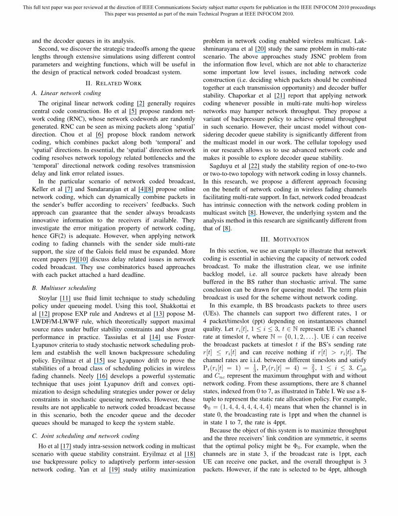
Fig. 2. Evolution of the receiver buffers at the beginning of the corresponding timeslot without (a) and with (b) network coding.
UE 1 can receive nothing, the other UEs can receive 4 packetseach. The total throughput is 8 packets. It is easy to calculatethat the average rate for each UE when the BS selects policyΦ0 is C0 = 73
27ppt. However, we shall show that this optimalthroughput cannot be achieved without network coding.
Assume that the channel state sequence is (6, 6, 5, 5, 3,3, 4, 2, 1, · · · ). Fig. 2(a) illustrates the evolution process ofthe receivers’ buffer without network coding. We can see thatthere is a 4-packet hole for each receiver at the beginning oftimeslot 9. Unless sacrificing throughput, these holes cannotbe filled because the average occurrence probability of states3, 5, 6 are twice the probability of the states 1, 2, 4. However,these holes can be filled by performing network coding whenneeded, as illustrated in Fig. 2(b). At the beginning of timeslot4, UE 2 possesses packet 1–8 and needs packet 9–16 while UE3 possesses packet 9–16 and needs 1–8. If there is no networkcoding, the BS can only send packet 17–20 which are novelfor both UE 2 and 3. When network coding is allowed, theBS can send the XOR of packet 1–4 and packet 9–12.
TABLE ICHANNEL VARIATION PROBABILITY
Seq. r1 r2 r3 Probability
0 1 1 1 1/271 1 1 4 2/272 1 4 1 2/273 1 4 4 4/274 4 1 1 2/275 4 1 4 4/276 4 4 1 4/277 4 4 4 8/27
Since plain broadcast policy has to fill those holes, whichresults in throughput loss. We can calculate its maximalthroughput Cpb = 65
27 < C0 = Cnc. Note that the abovethroughput improvement of network coding is not related tochannel error but due to multiuser diversity.
The above example illustrates that network coding is nec-essary to achieve maximum throughput in downlink wirelessbroadcast. However, the infinite backlog model hides thequeue stability related issues. In this research, we carry outa thorough study of this problem using queueing model.
IV. PROBLEM FORMULATION
A. System model
The downlink broadcast model used in this paper is illus-trated in Fig. 1, where a BS broadcasts packets to N UEs,
indexed from 1 to N . We assume the MAC layer encoding anddecoding operation is transparent to the upper layers. Thus,when network coded packets are received by a UE, they arestored in the UE’s decoder buffer. When the decoder is ableto decode the buffered packets, it decodes and forwards thosepackets to upper layers immediately.
The system operates in discrete time. A time interval [t, t+1), t ∈ N is called timeslot t. Denote by a[t] the numberof packets arrived in slot t. All arrivals in slot t happen atthe time instant t and are available for service in slot t, butare not counted into the queue length at slot t. The channelstates of different timeslots are i.i.d. The number of channelstate is finite and its stationary distribution is denoted by π =(π1, π2, . . . , πM ). The sender can choose its sending rate froma bounded set S ∈ N. The sending rate is integer because itrepresents the number of packets broadcasted in that timeslot.Let p
(m)i (μ) denote UE i’s average packet delivery ratio when
the channel is in state m and the BS broadcasts packets usingrate μ ∈ S.
The BS knows exactly whether or not a particular packethas been received by UE i through feedback. Assume thateach source packet is tagged with an integer sequence numberstarting from 0. μ[t] denotes the broadcast rate at timeslot t.Each timeslot t is divided into μ[t] sub timeslots, indexed by(t, l), 0 ≤ l < μ[t], which represents the interval [t + l
μ[t] , t +l+1μ[t] ), (t, μ[t]) = (t + 1, 0) = t + 1. In each sub timeslot,
BS sends one packet. Let σ(m)i,μ [t, l] be a 0-1 indicator which
represents whether or not the packet sent at sub timeslot (t, l)is successfully received by UE i when the channel is in statem with sending rate μ. We have E[σ(m)
i,μ [t, l]] = p(m)i (μ).
Definition 1: [Convolutional Random Network Coding]The packet sent in sub timeslot (t, l) using CRNC is specifiedas:
P [t, l] =N∑
i=1
ci[t, l] · PNexti[t,l] (1)
where PNexti[t,l] is the source packet indexed by Nexti[t, l].Nexti[t, l] is the next sequence number expected by UE iat sub timeslot (t, l). The meaning of Nexti[t, l] will beclear later. PNexti[t,l] is seen as a vector over Galois fieldGF (2D), D ≥ 1 by grouping every D bits together torepresent one symbol in GF (2D). ci[t, l] is randomly selectedfrom GF (2D). ci[t, l] = 0 if p
(m)i (μ[t]) = 0 or PNexti[t,l]
is unavailable. All addition and multiplication operations in
This full text paper was peer reviewed at the direction of IEEE Communications Society subject matter experts for publication in the IEEE INFOCOM 2010 proceedingsThis paper was presented as part of the main Technical Program at IEEE INFOCOM 2010.
Next[t,l+1]wi[t,l]
Un-decoded Pkt
dec_bufi[t,l]
Next[t,l]
a[k]xi[t,l]
x[t,l]
Pkt ready for scheduling
Nexti[t,l]
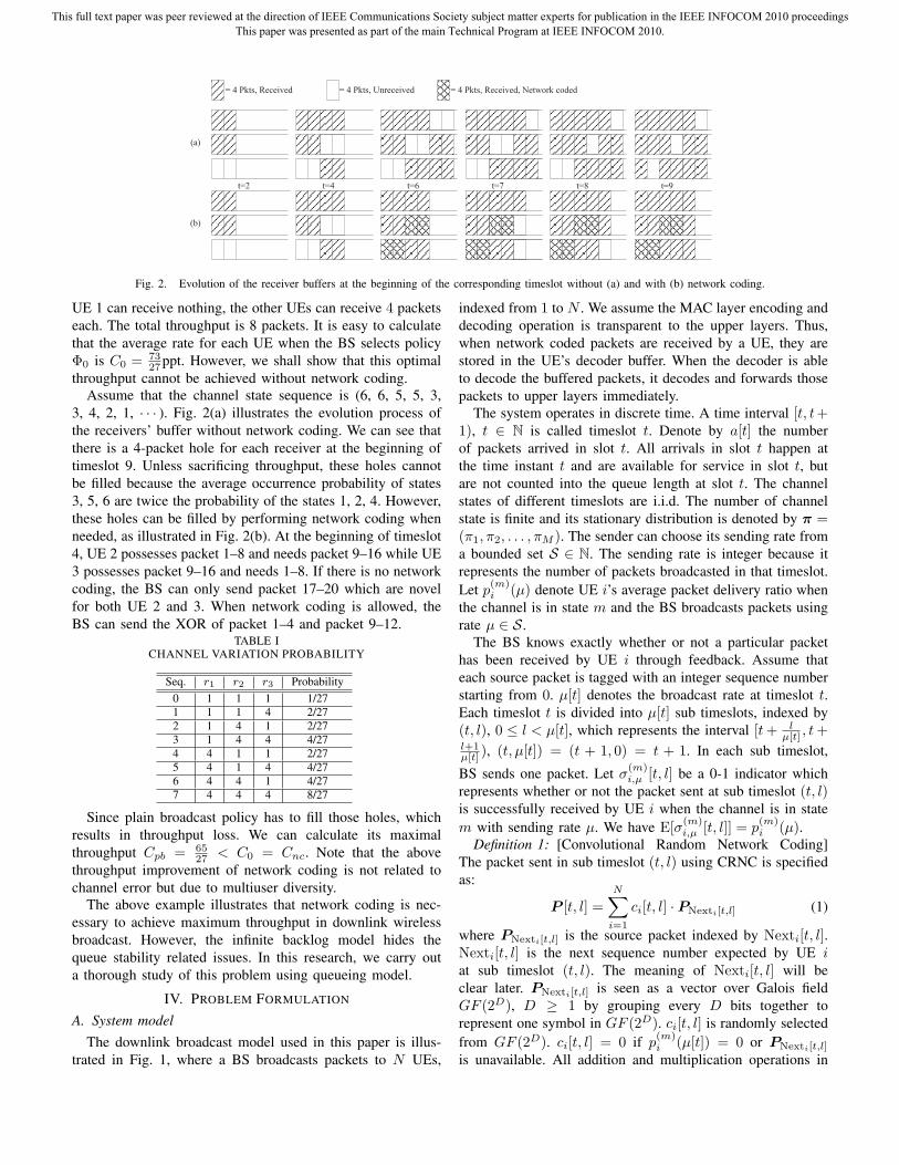
(a) (b)Fig. 3. Illustration of BS’s queue (a) and UEs’ queues (b).
n1 nNn2c1 cNc2
#m ... #m+2#m+1dec_bufi
=
received packet = ...
...
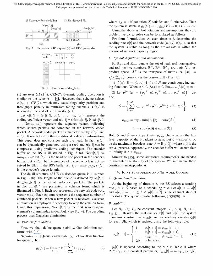
Fig. 4. Illustration of dec bufi.
(1) are over GF (2D). CRNC’s dynamic coding operation issimilar to the scheme in [4]. However, that scheme selectsci[t, l] ∈ GF (2), which may cause singularity problem andthroughput penalty in multi-rate fading channels. P [t, l] isreceived at the end of sub timeslot (t, l).
Let c[t, l] = (c1[t, l], c2[t, l], . . ., cN [t, l]) represent thecoding coefficient vector and n[t, l] = (Next1[t, l], Next2[t, l],· · · , NextN [t, l]) represent the sequence vector, indicatingwhich source packets are combined in the network codedpacket. A network coded packet is characterized by c[t, l] andn[t, l]. It needs to store these additional codeword information.This paper does not consider such overhead. In fact, c[t, l]can be dynamically generated using a seed and n[t, l] can becompressed using predictive coding techniques. The encoderbuffer at the BS is illustrated in Fig. 3 (a). Next[t, l] :=min1≤i≤NNexti[t, l] is the head of line packet in the sender’sbuffer. Let xi[t, l] be the number of packet which is not re-ceived by UE i in the BS’s buffer. x[t, l] := max1≤i≤Nxi[t, l]is the encoder’s queue length.
The detail structure of UE i’s decoder queue is illustratedin Fig. 3 (b). The length of the queue is denoted by wi[t, l].dec bufi[t, l] is the set of undecoded packets. The packetsin dec bufi[t, l] are presented in echelon form, which isillustrated in Fig. 4. Each row represents the network codewordvector c[t, l]. Each column represents the sequence number ofcombined packets. When a new packet is received, Gaussianelimination is employed if necessary to keep the echelon form.Using this expression, Nexti[t, l] is the first zero diagonalelement’s column index in dec bufi (see Fig. 4). The decodingprocess uses Gaussian elimination.
B. Problem formulation
First, we shall define queue stability. Our definition con-forms with [16].
Definition 2: [Queue length stability] Let overflow functionfor queue f be
gf (V ) = lim supt→∞
E(1t
t−1∑i=0
1f [t]>V ) (2)
where 1X = 1 if condition X satisfies and 0 otherwise. Thenthe system is stable if gx(V ) → 0, gwi
(V ) → 0, as V → ∞.Using the above symbol notations and assumptions, the core
problem we try to solve can be formulated as follows.Problem formulation: At each timeslot t, determine the
sending rate μ[t] and the network code (n[t, l], c[t, l]), so thatthe system is stable as long as the arrival rate is within theinterior of network capacity region.
C. Symbol definitions and assumptions
R, R+, and R++ denote the set of real, real nonnegative,and real positive numbers. R
N , RN+ , R
N++ are their N -times
product space. AT is the transpose of matrix A. ‖x‖ :=√∑Ni=1 x2
i . conv(X ) is the convex hull of set X .
1) fi(x): R → [0,∞), 1 ≤ i ≤ N are continuous, increas-ing functions. When x ≤ 0, fi(x) = 0, limx→∞ fi(x) = ∞;
2) Let p(m)(μ) =(p(m)1 (μ), p(m)
2 (μ), . . . , p(m)N (μ)
)T
, de-fine
S =
{M∑
m=1
πm · μ(m) · p(m)(μ(m)), μ(m) ∈ S}
(3)
μmax = sup{
mini{ηi}|η ∈ conv(S)
}(4)
ηi = sup{ηi|η ∈ conv(S)
}(5)
Both S and S are compact sets, μmax characterizes the linklayer capacity of the broadcast system. Let η = supS < ∞be the maximum broadcast rate, λ = E(a[0]), where a[t] is thearrival process. Apparently, the encoder buffer will accumulateto infinity if λ > μmax.
Similar to [15], some additional requirements are neededto guarantee the stability of the system. We summarize theseconstraints in Appendix A.
V. JOINT SCHEDULING AND NETWORK CODING
A. Queue length evolution
At the beginning of timeslot t, the BS selects a sendingrate μ[t] ∈ S based on a scheduling rule. Let a[t, 0] = a[t]and a[k, l] = 0, 1 ≤ l < μ[t]. m[t] is the channel state attimeslot t. The queues evolve following (7)(8)(9)(10).
B. Stability
Let B1, B2, B3 be constant integers, B1 > η, B2 > 0,B3 ≥ 0. Besides the real queues x[t] and w[t], the systemmaintains a virtual queue yi[t] and an auxiliary variable ζi[t]for each UE, which is updated using the following rule:
ζi[t + 1] =
⎧⎪⎪⎨⎪⎪⎩
1 xi[t + 1] = xmin[t + 1];0 xi[t + 1] = xmax[t + 1],
xmin[t + 1] �= xmax[t + 1];ζi[t] otherwise.
(11)
yi[t] is updated according to the rule in Table II whereΔ ∈ R++ is a constant parameter, xmin[t] = min1≤i≤Nxi[t],
This full text paper was peer reviewed at the direction of IEEE Communications Society subject matter experts for publication in the IEEE INFOCOM 2010 proceedingsThis paper was presented as part of the main Technical Program at IEEE INFOCOM 2010.
xi[t, l + 1] = xi[t, l] + a[t, l] − σ(m[t])i,μ[t] [t, l]Φ(n[t, l], c[t, l], dec bufi[t, l]) (7)
Nexti[t, l + 1] = Nexti[t, l] + σ(m[t])i,μ[t] [t, l]Φ(n[t, l], c[t, l], dec bufi[t, l]) (8)
dec bufi[t, l + 1] =
{dec bufi[t, l]
⋃(n[t, l], c[t, l]) if σ
(m[t])i,μ[t] [t, l] = 1;
dec bufi[t, l] if σ(m[t])i,μ[t] [t, l] = 0.
(9)
Φ(n[t, l], c[t, l],dec bufi[t, l]) ={
0 if rank(dec bufi[t, l]⋃
(n[t, l], c[t, l])) = rank(dec bufi[t, l])1 if rank(dec bufi[t, l]
⋃(n[t, l]), c[t, l])) = rank(dec bufi[t, l]) + 1.
(10)
TABLE IIyi[t]’S UPDATE RULE
i = 1 0
i > 1
ζi[t] = ζ1[t] yi[t]ζi[t] = 1, ζ1[t] = 0 yi[t] − Δ1
a
ζi[t] = 0, ζ1[t] = 1xi[t] < η yi[t]xi[t] ≥ η yi[t] + Δ2
b
aΔ1 = min(xmax[t] − xi[t], Δ)bΔ2 = min(xi[t] − xmin[t], Δ)
xmax[t] = max1≤i≤Nxi[t], y[0] ∈ RN , y1 ≡ 0, ζ[0] ∈
{0, 1}N . Let D[t] be the set with maximum dec bufi[t, 0]:
D[t] = arg max1≤i≤N
{wi[t] + xi[t] − x[t]} (12)
Definition 3: [Bidirectional Pressure Policy] Let τ [0] = 0,wmax[t] = max1≤i≤N (wi[t]). At the beginning of timeslot t:
1) If max1≤i≤N (xi[t] + yi[t]) < B1 and wmax[t] > B2, orτ [t] > 0, the BS selects its broadcast rate μ[t] as:
μ[t] ∈ agrmaxη∈S{η · p(m)i (η), i ∈ D[t]} (13)
Let D′[t] = {i|p(m)i (μ[t]) = maxj∈D[t] p
(m)j (μ[t]), i ∈ D[t]},
the broadcast packet is encoded as:
P [t, l] =∑
i∈D′[t]
ci[t, l] · PNexti[t,l] (14)
τ [t + 1] ={
τ [t] − 1 τ [t] > 0;B3 τ [t] = 0.
(15)
2) If max1≤i≤N (xi[t] + yi[t]) ≥ B1 or wmax[t] ≤ B2, andτ [t] = 0, μ[t] is determined by:
μ[t] ∈ arg maxη∈S
{N∑
i=1
fi(xi[t] + yi[t]) · min(η · p(m)i (η), xi[t])}
(16)In each sub slot (t, l), CRNC (1) is used to construct the
broadcasting packets, τ [t + 1] = 0. We call the combinationof CRNC and BiP scheduling policy as JSNC.
The main result of this paper is summarized in Theorem 1,which characterizes the stability property of the JSNC policy.
Theorem 1: If JSNC is used in every timeslot t, λ <μmax(1 − ε), D >
⌈log N
ε
⌉, B3 > η
ηi−λ� − 1, ε ∈ R++.Then ∃Δ0, as long as 0 < Δ ≤ Δ0, both x[t] and w[t] arestable.
Proof: Formal proof is included in Appendix A.We give an intuitive explanation of the JSNC policy. We
first discuss policy (16). Note that the UE corresponding to
1
0 maxxminx
1ix 2i
x
4ix
3ix
0
Fig. 5. Visualization of yi[t]’s update rule.
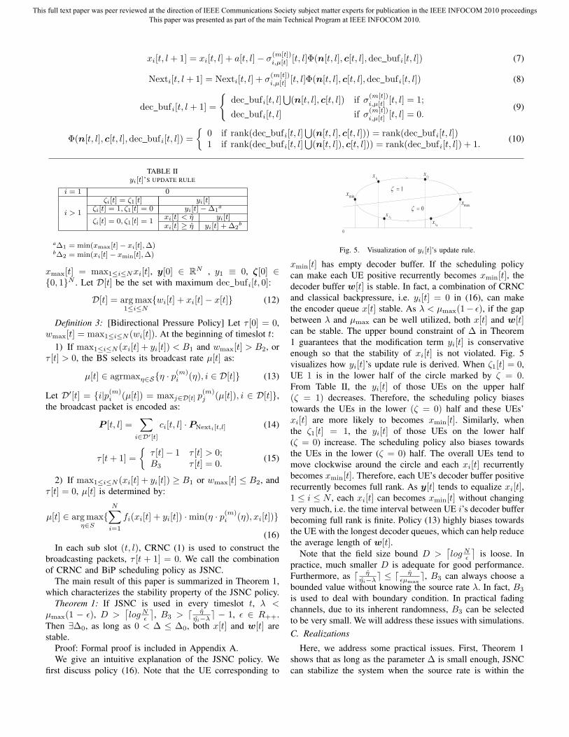
xmin[t] has empty decoder buffer. If the scheduling policycan make each UE positive recurrently becomes xmin[t], thedecoder buffer w[t] is stable. In fact, a combination of CRNCand classical backpressure, i.e. yi[t] = 0 in (16), can makethe encoder queue x[t] stable. As λ < μmax(1− ε), if the gapbetween λ and μmax can be well utilized, both x[t] and w[t]can be stable. The upper bound constraint of Δ in Theorem1 guarantees that the modification term yi[t] is conservativeenough so that the stability of xi[t] is not violated. Fig. 5visualizes how yi[t]’s update rule is derived. When ζ1[t] = 0,UE 1 is in the lower half of the circle marked by ζ = 0.From Table II, the yi[t] of those UEs on the upper half(ζ = 1) decreases. Therefore, the scheduling policy biasestowards the UEs in the lower (ζ = 0) half and these UEs’xi[t] are more likely to becomes xmin[t]. Similarly, whenthe ζ1[t] = 1, the yi[t] of those UEs on the lower half(ζ = 0) increase. The scheduling policy also biases towardsthe UEs in the lower (ζ = 0) half. The overall UEs tend tomove clockwise around the circle and each xi[t] recurrentlybecomes xmin[t]. Therefore, each UE’s decoder buffer positiverecurrently becomes full rank. As y[t] tends to equalize xi[t],1 ≤ i ≤ N , each xi[t] can becomes xmin[t] without changingvery much, i.e. the time interval between UE i’s decoder bufferbecoming full rank is finite. Policy (13) highly biases towardsthe UE with the longest decoder queues, which can help reducethe average length of w[t].
Note that the field size bound D >⌈log N
ε
⌉is loose. In
practice, much smaller D is adequate for good performance.Furthermore, as η
ηi−λ� ≤ ηεμmax
�, B3 can always choose abounded value without knowing the source rate λ. In fact, B3
is used to deal with boundary condition. In practical fadingchannels, due to its inherent randomness, B3 can be selectedto be very small. We will address these issues with simulations.
C. Realizations
Here, we address some practical issues. First, Theorem 1shows that as long as the parameter Δ is small enough, JSNCcan stabilize the system when the source rate is within the
This full text paper was peer reviewed at the direction of IEEE Communications Society subject matter experts for publication in the IEEE INFOCOM 2010 proceedingsThis paper was presented as part of the main Technical Program at IEEE INFOCOM 2010.
interior of S. However, from the visual explanation of JSNCin Fig. 5, there is a tradeoff between the update speed Δand the decoder buffer length wi[t]. If Δ is small, the speedof the clockwise movement along the circle decreases, thetime interval for a UE’s decoder buffer to become full rankincreases. Due to the weak connection between wi[t] and yi[t],the decoder buffers may become much larger than the encoderbuffer. To mitigate this issue, B1 and B2 are introduced.When B1 is big, B2 characterizes the tradeoff between theencoder queue length and decoder queue lengths. When B2
is small, the scheduler favors the decoder buffers so that theaverage decoder buffers are reduced. Otherwise, when B2 islarge, due to the conservative nature of Δ, in steady state,the decoder queues will be much longer than the encoderqueue. By properly selecting B2, without violating stability,the system’s average queue size can be reduced.
However, how to choose Δ and B2 are not explicitlyspecified in Theorem 1. In practice, we could dynamicallyadjust Δ and B2 so that the system is stable and the averagequeue lengths are small.
VI. SIMULATION
In this section, we investigate the performance of JSNCthrough simulation. Unless explicitly specified, we use thesettings as the example in Section III, so that we can compareour results with the theoretical value.
We primarily study two class of scheduling functions.
• Polynomial weighting (POLY),
fi(x) ={
xβ x ≥ 00 x < 0 , β > 0;
• Exponential weighting (EXP),
fi(x) ={
exκ − 1 x ≥ 00 x < 0
, 0 < κ < 1.
To emphasize on the benefit of JSNC, we assume that thereis no transmission error. The deliver probability satisfies:
p(m)i (μ) =
{0, μ ≥ μ
(m)i ;
1, μ < μ(m)i .
(17)
where μ(m)i is UE i’s supportable rate when its channel is in
state m. The BS’s and UEs’ buffer limits are 2000. The defaultvalues of the parameters in JSNC policy are Δ = 0.4, β = 1,κ = 0.5. The Galois field size is 256, B1 = 1000, B2 = 750,B3 = 0, the arrival process is deterministic, i.e. a[t] = λ.
A. Minimum rate, pure scheduling, and JSNC
In this subsection, we compare the performance of JSNCwith two other reference policies, named minimum ratescheduling and pure scheduling defined as follows.
1) Minimum rate: The BS chooses the minimum instaneouschannel rate among all users as transmitting rate.
2) Pure scheduling: The base station chooses a transmittingrate by the following policy,
μ[t] = arg maxη∈S
N∑i=1
fi(xi[t]) · η · p(m)i (η) (18)
Then it transmits packets with the minimum Nexti[t, l] amongthe users who can receive packets at that transmitting rate.Pure scheduling can be seen as a mimic of the backpressurescheduling to broadcast scenario.
In this subsection, we select POLY scheduling function.Besides the default configuration, we also adopt a more generalsetting: the number of user N is set to 5, the packet arrival rateis a constant, and the channel rate is chosen from a discreteset S = {1, 2, 3, 4, 5, 6, 7, 8} (ppt). For each UE, we generate7 random numbers from [0, 1], the corresponding 8 intervalsare set as the UE’s channel rate distribution.
The result is presented in Table III. EXA denotes the thechannel rate distribution specified by the example in SectionIII. RND i, 1 ≤ i ≤ 4 denotes the ith group of randomlygenerated channel rate distribution.
TABLE IIIMAXIMUM ARRIVAL RATE OF DIFFERENT SCHEDULING POLICY
Min Rate Pure scheduling JSNC
EXA 2.1 2.3 2.7RND 1 2.3 2.3 3RND 2 2.6 2.5 3.4RND 3 2.2 2.0 2.9RND 4 1.8 1.7 2.3
From Section III, we know that the capacity of EXA is7327 = 2.7037ppt. The simulation results show that JSNC cansupport an arrival rate ≥ 2.65ppt (take the rounding error intoaccount), which conforms to the conclusion of our analysis. Onaverage, comparing with min rate policy and pure schedulingpolicy, JSNC can achieve significant throughput gains at about20% ∼ 30%, respectively.
B. Impact of different parameters
This subsection discusses the impact of different form ofscheduling function fi(·), parameter Δ, and buffer thresholdB1, B2, B3.
1) Impact of scheduling functions: Fig. 6 shows CDF ofx1[t] and w1[t] using different weighting functions. OtherUE’s corresponding CDF curve behaves similarly. To showthe impact of different scheduling functions, we remove theeffect of the thresholds by setting B1 = B2 = 2000. Then(16) in Theorem 1 is always used. The source rate is fixed at2.5ppt, and we run 105 timeslots for each simulation. We cansee that for POLY weighting function, the encoder maintainsa small queue when the exponential coefficient β is small.The EXP weighting function approximately achieves the bestencoder queue length distribution. We can also see from thefigure that the decoder queue wi[t] is not sensitive to differentweighting functions. This phenomenon is due to the weakconnection between wi[t] and yi[t], which conforms to theintuitive explanation in the previous section.
2) Impact of Δ: Δ0 depends on the arrival rate. Table IVpresents Δ0 as a function of the arrival rate.
We can see that Δ0 increases when the arrival rate de-creases. From Appendix A, we can see that a large Δ cannotsupport large throughput due to the fact that, in this case, the
This full text paper was peer reviewed at the direction of IEEE Communications Society subject matter experts for publication in the IEEE INFOCOM 2010 proceedingsThis paper was presented as part of the main Technical Program at IEEE INFOCOM 2010.
0 10 20 30 40 500
0.2
0.4
0.6
0.8
1
CD
F o
f x1
x1
exp, η=0.5
β=1
β=2
β=3
0 100 200 3000
0.2
0.4
0.6
0.8
1
CD
F o
f w1
w1
exp, η=0.5
β=1
β=2
β=3
Fig. 6. CDF of x1[t] and w1[t] on different weighting coefficient.
TABLE IVΔ0 AS A FUNCTION OF λ.
λ 2.7 2.6 2.5 2.4Δ0 0.1 1 4 15
system spends too much time in the transient state and cannotconverge to the optimal operation point. Table IV verifies theseconclusions. From Section III, the capacity is 73
27 = 2.704ppt.The simulation conforms that JSNC can supports up to 2.7pptwhen Δ ≤ 0.1. The loss of 0.004ppt is primarily due to finitebuffer size and the finite field size (i.e. 28).
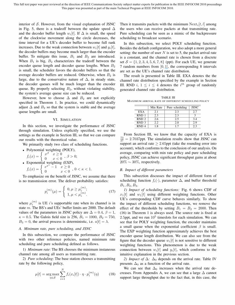
3) Impact of the encoder queue’s threshold: We found thatwhen B1 is chosen properly large and B3 is chosen properlysmall, the queue length distribution is not sensitive to these twovalues. This subsection investigates the relationship betweenthe threshold B2 and the queue length distributions by fixingB1 = 1000 and B3 = 0. The packet arrival rate is fixed at2.5ppt. Fig. 7 shows the CDF of BS’s and UEs’ queue lengthson different threshold. When the threshold grows, the BS’squeue decreases and the UEs’ queues increase, i.e. there is atradeoff between the encoder queue and the decoder queues. Infact, the policy (13)(14) bias to decoder queues while (16)(1)reacts slowly to the increase of the decoder queue. Therefore,B2 can approximately be seen as the switch point of these twopolicies.
VII. CONCLUSION
In this research, we have developed a joint scheduling andnetwork coding scheme to support stable maximum throughputbroadcast in wireless fading channels. This scheme is fun-damentally different from existing network coded broadcastsystems in that maximum throughput broadcast is accom-plished with multi-rate transmission and under the stable queueconstraints at both base station and receivers. Both theoreticalanalysis and experimental simulations have been carried outto verify the performance of the proposed JSNC scheme.
The model used in this research requires the BS to beaware of each UE’s status. We did not discuss the overheadof collecting this information. In practice, when the numberof UE becomes large, such overhead cannot be omitted.To mitigate this difficulty, studying the impact of delayedfeedback to network throughput is an important future work.
APPENDIX A
In this proof, we assume that the set S is strictly convex.This assumption is not in essential, as long as S is convex,
0 20 40 60 800
0.2
0.4
0.6
0.8
1
BS Queue Length
CD
F
TH=250TH=200TH=150TH=100TH=75TH=50
0 50 100 1500
0.2
0.4
0.6
0.8
1
UE Queue Length
CD
F
TH=250TH=200TH=150TH=100TH=75TH=50
Fig. 7. CDF of UEs queue length and BS queue length on different threshold.
Theorem 1 holds. However, the strict convexity of S simplifiesthe proof.
First we study deterministic model, and assumethat the Galois field size is big enough so thatΦ(n[t, l], c[t, l], dec bufi[t, l]) ≡ 1. Both the arrival processand channel rate process are deterministic, i.e. a[t] = λand the sending rate is chosen from S. At the beginningof each timeslot t, if max1≤i≤N (xi[t] + yi[t]) ≥ B1 ormax1≤i≤Nwi[t] ≤ B2, and τ [t] = 0, the sender selects itsrate μ[t] according to:
μ[t] ∈ arg maxη
{N∑
i=1
fi(xi[t] + yi[t]) ·min(ηi[t], xi[t]),η ∈ S}(19)
and encode the packet using (1), τ [t + 1] = 0. Otherwise thescheduling rule is
μ[t] ∈ arg maxη∈S
{ηi, i ∈ D[t]} (20)
From the strictly convexity of S, if (20) is used, there is onlyone nonzero component in μ[t]. Denote the UE correspondingto this element as I[t]. The broadcasted packet is PNextI[t][t,l],τ [t] is updated according to (15).
We now prove that the above policy is stable as long asλ < μmax.
Let 1N = (1, 1, . . . , 1)T be a dim-N vector, gi(z) = fi(z),L(z) =
∑Ni=1 gi(zi). Define Δmax := inf{‖λ · 1N − η‖ ,η ∈
S}. As S is convex and compact, λ is within the interior ofS, we have Δ > 0. From Taylor’s theorem, ∃zi[t] betweenxi[t + 1] + yi[t + 1] and xi[t] + yi[t],
gi(xi[t + 1] + yi[t + 1]) − gi(xi[t] + yi[t])= fi(zi[t])(xi[t + 1] + yi[t + 1] − xi[t] − yi[t]) (21)
Further, from the strictly convex of S and (19), xmax[t] ≥η ⇒ xi[t] ≥ μi[t]. Select Δ < Δmax
2√
N, when ‖f(x[t])‖ > 0
ΔL(x[t] + y[t]) � L(x[t + 1] + y[t + 1]) − L(x[t] + y[t])
=N∑
i=1
fi(zi[t])(xi[t + 1] − xi[t] + yi[t + 1] − yi[t])
=N∑
i=1
fi(zi[t])(λ − μi[t]) +N∑
i=1
fi(zi[t])(yi[t + 1] − yi[t])
Let E [t] = {i|1 ≤ i ≤ N,xi[t] < η}, Δ[t] is a N -dimension
vector with Δi[t] ={
Δ i /∈ E [t]0 i ∈ E [t] , then the point λ · 1N +
This full text paper was peer reviewed at the direction of IEEE Communications Society subject matter experts for publication in the IEEE INFOCOM 2010 proceedingsThis paper was presented as part of the main Technical Program at IEEE INFOCOM 2010.
Δ[t] is strictly between the two hyper planes accross λ1N andμ[t] respectly with slop ϕi[t] = fi(zi[t])
‖f(z[t])‖ . We have
N∑i=1
ϕi[t]μi[t] −N∑
i=1
ϕi[t]λ >N∑
i=1
ϕi[t](λ + Δi[t]) −N∑
i=1
ϕi[t]λ
⇒N∑
i=1
ϕi[t](λ + Δi[t]) −N∑
i=1
ϕi[t]μi[t] < 0 (22)
ΔL(x[t] + y[t])
≤ ‖f(z[t])‖(
N∑i=1
ϕi[t](λ − μi[t]) +N∑
i=1
ϕi[t]Δi[t]
)< 0
Therefore, ∃C1 ∈ R++,
L(x[t] + y[t]) = g1(x1[t]) +N∑
i=2
gi(xi[t] + yi[t]) < C1 (23)
We can draw the following three assertions.
Assertion 1. ∃Tmax < ∞, ∀t, ∃0 < T ≤ Tmax,dec buf1[t + T ] is full rank.
If ∀t, ζ1[t] ≡ 0, then unless xmax[t] = xmin[t], x1[t] �=xmin[t], UE 1’s decoder buffer is never full rank. If thescheduler never choose rule (19), there are two cases:
• If UE 1 is never scheduled, x1[t + 1] − x1[t] = λ, i.e.x1[t] → ∞. From (23), x1[t] ≤ g−1
1 (C1), we get acontradiction.
• ∃t0 < ∞, UE 1 is scheduled. From (12), ∀2 ≤ i ≤ N ,UE 1’s decoder buffer length at t0 + 1 satisfies:
w1[t0 + 1] + x1[t0 + 1] − x[t0 + 1]= (w1[t0] + x1[t0] − x[t0]) + μ1[t0]> (wi[t0] + xi[t0] − x[t0]) + μi[t0]= wi[t0 + 1] + xi[t0 + 1] − x[t0 + 1] (24)
Therefore, only UE 1 is scheduled for ∀t > t0. As λ iswithin the interior of S, ∃T < ∞, x1[t0 + T ] = 0 =xmin[t0 + T ], we also get a contradiction.
Then (19) is recurrently trigged. The interval between succes-sive trigger is bounded by
T1 =⌈g−11 (C1)
(1λ
+1
ηi − λ
)+ 2⌉
(25)
When (19) is used, from Table II,
N∑i=1
yi[t + 1] −N∑
i=1
yi[t] < 0 (26)
From the strictly convexity of S, if xi[t] + yi[t] < 0,wmax[t] > B2, and (19) is used, then μi[t] = 0. From (26),∃2 ≤ i0 ≤ N , t0 ∈ R+, yi0 [t0] < −g−1
1 (C1)− η. So ∀t ≥ t0,xi0 [t] > g−1
1 (C1) ≥ x1[t]. This conclusion means that ifζi[t] = 1, after a bounded time interval, xi[t] > x1[t]. ∀t, ifxmin[t] �= xmax[t], {i|ζi[t] = 1} �= φ, so ∃t, x1[t] = xmin[t],
we get a contradiction. From the above explanation, the timeinterval of x1[t] becomes xmin[t] is upper bounded by
T2 = T1 ·(N∑
i=2
⌈2g−1
i (C1) + η
Δ+ 1⌉
+⌈
B2 + g−11 (C1)λ
+ 1⌉)
(27)If ∀t, ζ1[t] ≡ 1, due to the same reason as illustrated
before, the scheduler cannot continuously choose rule (20)more than T1 timeslots. When (19) is used and xmax[t] ≥ η,
N∑i=1
yi[t + 1] −N∑
i=1
yi[t] > 0 (28)
Similar to the induction for the case of ζ1[t] = 0, the systemcannot stay in the state xmax[t] ≥ η more than T2 timeslots.If the system stays in the state with xmax[t] < η and (19) isalways selected, from (23) and the fact that when ζ1[t] ≡ 1,yi[t] are nondecreasing. Let
L1 ={
x + y
∣∣∣∣ 0 ≤ xi < η, yi ≥ −η, L(x + y) < C1,max1≤i≤N (xi + yi) ≥ B1
}After no more than |L1| timeslots, x1[t] = 0 = xmin[t].Therefore, (20) is chosen recurrently. Once (20) is chosen,the rule will be used with at least B3 continuous timeslots.As B3 + 1 > η
ηi−λ�, one UE’s decoder buffer will becomefull rank. As N is finite, UE 1’s decoder queue will becomesfull rank. We get a contradiction. The time interval of ζ1[t] tobecomes 0 is upper bounded by
T3 = T2 · |L1| · N · (B3 + 1) (29)
Let Tmax = T2 + T3, Assertion 1 holds.Assertion 2. ∃C2 ∈ R++, ∀t, max1≤i≤N |yi[t]| < C2,
xmax[t] < C2.From Assertion 1, x1[t] recurrently becomes xmax[t]
within a bounded period and x1[t] ≤ g−11 (C1). Let
C2 =N∑
i=1
g−1i (C1) + λ · Tmax + η (30)
Assertion 2 satisfies.Assertion 3. w[t] is bounded.If ∃wi[t] → ∞, and (19) is never triggered, similar to
the illustration in Assertion 1, UE i’s decoder needs at mostT4,1 =
⌈C2
(1λ + 1
ηi−λ
)+ 1⌉
timeslots to become full rank.So (19) is recurrently triggered. There are two cases:
• (20) is never used.If ∀t, ζi[t] ≡ 0, after each time interval of UE 1 becomesxmin[t] → xmax[t] → xmin[t], unless xi[t] < η, yi[t]increase. However, yi[t] cannot increase to arbitrarily largedue to (23). UE i can also not always stays within the statexi[t] < η because in this case L(x[t]+y[t]) decrease. Let
L2 = {x+y||xi| < C2, |yi| < C2, max1≤i≤N
(xi +yi) ≥ B1}
Then |L2| is finite. xi[t] becomes xmin[t] within a timeinterval of
T4,2 = (⌈
C2 + B2
λ+ 1⌉+|L2|)·
⌈2C2
Δ+ 1⌉·Tmax (31)
This full text paper was peer reviewed at the direction of IEEE Communications Society subject matter experts for publication in the IEEE INFOCOM 2010 proceedingsThis paper was presented as part of the main Technical Program at IEEE INFOCOM 2010.
If ∀t, ζi[t] ≡ 1, after each round of UE 1, yi[t] decreases.Because xi[t] ≥ −yi[t] − η, xi[t] → ∞, which contra-dicts with Assertion 2. Therefore, each ζi[t] recurrentlybecomes 0 within a bounded interval
T4,3 =⌈
2C2
Δ+ 1⌉· Tmax (32)
• Both (19) and (20) are recurrently triggered.The induction of this case is similar to the above, UE i’sdecoder buffer needs at most
T4 = T4,1 · (T4,2 + T4,3) · N · (B3 + 1) (33)
timeslots to become full rank.From Assertion 2 and 3, Theorem 1 holds for deterministic
model. Extending the deterministic model to stochastic modelneeds the following additional constraints.
1) ∀M1,M2 ∈ R++, 0 < ε < 1, ∃B ∈ R+, ∀x > B,(1 − ε)fi(x) ≤ fi(x − M1) ≤ fi(x + M2) ≤ (1 − ε)fi(x).
2) Let μ(m,x,y) be the sending rate when channel is instate m with encoder queue vector x and virtual queue vectory. ∀A, ε ∈ R++, ∃B ∈ R++, such that for ∀x1,x2 ∈ R
N+ ,
y1,y2 ∈ RN that satisfies ‖x1 + y1‖ , ‖x2 + y2‖ < B, and
|x1,i − x2,i| , |y1,i − y2,i| < A, we have:∣∣∣∣N∑
i=1
fi(x1,i + y1,i)μ(m,x1,y1)p(m)i (μ(m,x1,y1))−
N∑i=1
fi(x2,i + y2,i)μ(m,x2,y2)p(m)i (μ(m,x2,y2))
∣∣∣∣< ε
N∑i=1
fi(x1,i + y1,i)μ(m,x1,y1)p(m)i (μ(m,x1,y1))
3) The arrival process a[t] is i.i.d. between different slots.It satisfies limA→∞ Afi(A)Pr(a[t] > A) = 0.
The proof can be done using the large number theory basedtechnology in [15] or fluid limit technology in [12]. The detailis similar to [15] and we omit it due to page limit.
Now we analyze the throughput loss due to finite field size,i.e. Φ(n[t, l], c[t, l],dec bufi[t, l]) = 0. At each sub timeslot,the probability of sending a non-novel network coded packetto UE i is maximized when the dimension of dec bufi[t, l] isK and its rank is K − 1. The corresponding probability is
2D(K−1)
2DK= 2−D (34)
We have:
Pr(Φ(n[t, l], c[t, l],dec bufi[t, l]) = 0) ≤ 2−D (35)
Therefore, as long as D >⌈log2
Nε
⌉, i.e. ε > N2−D, the
rate region considering such loss, denoted by αS satisfies:
α ≥ 1 −N∑
i=1
Pr(Φ(n[t, l], c[t, l],dec bufi[t, l]) = 0)
≥ 1 − N2−D > 1 − ε (36)
From the condition of λ < (1−ε)μmax, Theorem 1 holds. Notethat in this scenario, Δmax = inf
{‖λ · 1N − η‖ ,η ∈ αS}.
REFERENCES
[1] R. Ahlswede, N. Cai, S.-Y. R. Li, and R. W. Weung, “Networkinformation flow,” IEEE Trans. Inf. Theory, vol. 46, no. 4, pp. 1204–1216, Jul. 2000.
[2] S.-Y. R. Li, R. W. Yeung, and N. Cai, “Linear network coding,” IEEETrans. Inf. Theory, vol. 49, no. 2, pp. 371–381, Jul. 2003.
[3] A. Eryilmaz, A. Ozdaglar, and M. Medard, “On delay performance gainsfrom network coding,” in Proc. 40th Annu. IEEE Conf. Inform. Sci. Syst.(CISS’06), Princeton, NJ, USA, Mar. 22–24, 2006, pp. 864–870.
[4] J. K. Sundararajan, D. Shah, and M. Medard, “ARQ for network coding,”in Proc. 2008 IEEE Int. Symp. Inf. Theory (ISIT’08), Toronto, Ontario,Canada, Jul. 6–11, 2008.
[5] T. Ho, M. Medard, , R. Koetter, D. R. Karger, M. Effros, J. Shi, andB. Leong, “A random linear network coding approach to multicast,”IEEE Trans. Inf. Theory, vol. 52, no. 10, pp. 4413–4430, Oct. 2006.
[6] P. A. Chou, Y. Wu, and K. Jain, “Practical network coding,” in Proc.41st Allerton Conf. Commun., Contr., and Computing, Monticello, IL,USA, Oct. 1–3, 2003.
[7] L. Keller, E. Drinea, and C. Fragouli, “Online broadcasting with networkcoding,” in Proc. 4th IEEE Workshop on Network Coding, Theory, andApplications (NetCod’08), HK, China, Jan. 3–4, 2008.
[8] J. K. Sundararajan, M. Medard, M. Kim, A. Eryilmaz, D. Shah, andR. Koetter, “Network coding in a multicast switch,” in Proc. 26th Annu.IEEE Conf. Comput. Commun. (INFOCOM’07), Anchorage, Alaska,USA, May 6–12, 2007, pp. 1145–1153.
[9] W.-L. Yeow, A. T. Hoang, and C.-K. Tham, “Minimizing delay formulticast-streaming in wireless networks with network coding,” in Proc.28th Annu. IEEE Conf. Comput. Commun. (INFOCOM’09), Rio deJaneiro, Brazil, Apr. 19–25, 2009.
[10] J. Barros, R. A. Costa, D. Munaretto, and J. Widmer, “Effective delaycontrol in online network coding,” in Proc. 28th Annu. IEEE Conf.Comput. Commun. (INFOCOM’09), Rio de Janeiro, Apr. 19–25, 2009.
[11] A. L. Stolyar, “On the stability of multiclass queueing networks:A relaxed sufficient condition via limiting fluid processes,” MarkovProcesses and Related Fields, pp. 491–512, 1995.
[12] S. Shakkottai and A. L. Stolyar, “Scheduling for multiple flows sharinga time-varying channel: The exponential rule,” Analytic Methods inApplied Probability, American Mathematical Society Translations Series2, vol. 207, pp. 185–202, 2002.
[13] M. Andrews, K. Kumaran, K. Ramanan, A. Stolyar, R. Vijayakumar,and P. Whiting, “Scheduling in a queueing system with asynchronouslyvarying service rates,” Probability in the Engineering and InformationalSciences, vol. 18, pp. 191–217, 2004.
[14] L. Tassiulas and A. Ephremides, “Stability properties of constrainedqueueing systems and scheduling policies for maximum throughput inmultihop radio networks,” IEEE Trans. Autom. Control, vol. 37, no. 12,pp. 1936–1948, Dec. 1992.
[15] A. Eryilmaz, R. Srikant, and J. R. Perkins, “Stable scheduling policiesfor fading wireless channels,” IEEE/ACM Trans. Netw., vol. 13, no. 2,pp. 411–424, Apr. 2005.
[16] M. J. Neely, “Energy optimal control for time-varying wireless net-works,” IEEE Trans. Inf. Theory, vol. 52, no. 7, pp. 2915–2934, Jul.2006.
[17] T. Ho and H. Viswanathan, “Dynamic algorithms for multicast withintra-session network coding,” in Proc. 43rd Allerton Conf. Commun.,Contr., and Computing, Monticello, IL, US, Sep. 28–30, 2005.
[18] A. Eryilmaz and D. S. Lun, “Control for inter-session network coding,”in Proc. 3rd IEEE Workshop on Network Coding, Theory, and Applica-tions (NetCod’07), Jan. 29, 2007.
[19] X. Yan, M. J. Neely, and Z. Zhang, “Multicasting in time-varyingwireless networks: cross-layer dynamic resource allocation,” in Proc.2007 IEEE Int. Symp. Inf. Theory (ISIT’07), Jun. 24–29, 2007.
[20] S. Lakshminarayana and A. Eryilmaz, “Multi-rate multicasting withnetwork coding,” in Proc. 4th Annu. Int. Conf. Wireless Internet, Hawaii,USA, 2008.
[21] P. Chaporkar and A. Proutiere, “Adaptive network coding and schedulingfor maximizing throughput in wireless networks,” in Proc. 13th Annu.ACM Int. Conf. Mobile Comput. and Netw. (MobiCom’07), Montreal,Quebec, Canada, Sep. 9–14, 2007, pp. 135–146.
[22] Y. E. Sagduyu and A. Ephremides, “On broadcast stability region inrandom access through network coding,” in Proc. 44th Allerton Conf.Commun., Contr., and Computing, Monticello, IL, US, Sep. 27–29,2006.
This full text paper was peer reviewed at the direction of IEEE Communications Society subject matter experts for publication in the IEEE INFOCOM 2010 proceedingsThis paper was presented as part of the main Technical Program at IEEE INFOCOM 2010.