ARTICLE IN PRESS

Contents lists available at ScienceDirect

Signal Processing

Signal Processing 90 (2010) 145–156

0165-16

doi:10.1

$ The

Interna$$ T

Founda� Cor

E-m

ullrich.m

journal homepage: www.elsevier.com/locate/sigpro

Convergence behavior of non-equidistant sampling series$,$$

Holger Boche �, Ullrich J. Monich

Technische Universitat Berlin, Heinrich-Hertz-Chair for Mobile Communications, Einsteinufer 25, D-10587 Berlin, Germany

a r t i c l e i n f o

Article history:

Received 6 October 2008

Received in revised form

15 April 2009

Accepted 1 June 2009Available online 6 June 2009

Keywords:

Sampling series

Sine type

Non-equidistant sampling

Reconstruction

Stochastic process

84/$ - see front matter & 2009 Elsevier B.V. A

016/j.sigpro.2009.06.003

material in this paper was presented in pa

tional Conference on Acoustics, Speech, and Si

his work was partly supported by the

tion (DFG) under Grant BO 1734/9-1.

responding author.

ail addresses: holger.boche@mk.tu-berlin.de (

oenich@mk.tu-berlin.de (U.J. Monich).

a b s t r a c t

The convergence of sampling series with non-equidistant sampling points cannot be

guaranteed for the Paley–Wiener space PW1p if the class of sampling patterns is not

restricted. In this paper we consider sampling patterns that are made of the zeros of

sine-type functions and analyze the local and global convergence behavior of the

sampling series. It is shown that oversampling is necessary for global uniform

convergence. If no oversampling is used there exists for every sampling pattern a

signal such that the peak value of the approximation error grows arbitrarily large.

Furthermore, we use the findings to derive results about the mean-square convergence

behavior of the sampling series for bandlimited wide-sense stationary stochastic

processes. Finally, a procedure is given to construct functions of sine type and possible

sampling patterns.

& 2009 Elsevier B.V. All rights reserved.

1. Notation and motivation

The reconstruction of bandlimited signals from theirsamples is important for many applications in signalprocessing, communication, and information theory. TheShannon sampling series

X1k¼�1

f ðkÞsinðpðt � kÞÞ

pðt � kÞ(1)

with sinc-kernel is probably the most prominent exampleof a reconstruction process. However, it is not the onlypossible one. In particular for practical applications, non-equidistant sampling patterns are of interest. In this case,more general sampling series can be used for thereconstruction, like

X1k¼�1

f ðtkÞfkðtÞ, (2)

ll rights reserved.

rt at the 2009 IEEE

gnal Processing [1].

German Research

H. Boche),

where fk, k 2 Z, are certain reconstruction functions, andftkgk2Z is the sequence of real sampling points.

There is a vast amount of literature discussing theproperties of sampling series with non-equidistant sam-pling points for the space of bandlimited signals withfinite energy: The papers [2,3] analyze the stability of suchsampling series, and [4] derives series representations.Sampling series involving derivatives are considered in[5], and the case where only a finite number of samplingpoints differs from the integer grid is considered in [6].Aspects of numerical computation in the reconstruction ofbandlimited signals with finite energy from irregularsamples are treated in [7,8].

Only few papers discuss non-equidistant sampling forlarger signal spaces than the space of bandlimited signalswith finite energy [9,10]. In [9] Seip proves the uniformconvergence of (2) on all compact subsets of the complexplane for bounded bandlimited signals if oversampling isused and the sequence ftkgk2Z of real sampling pointsfulfills

supk2Z

jtk � kj � D (3)

for some Do 14. Hinsen [10] analyzes (2) without over-

sampling for bandlimited signals that are in Lp, 1 � po1,when restricted to the real line. He gives a condition on D

ARTICLE IN PRESS

H. Boche, U.J. Monich / Signal Processing 90 (2010) 145–156146

which is sufficient for (2) to be uniformly convergent onall compact subsets of the complex plane.

In this paper we give a stronger result compared to theresult given in [9]. However, we obtain our result for adifferent sampling point sequence and for a smaller signalspace, namely PW1

p. Nevertheless, PW1p is still larger

than all spaces that were considered in [10], andespecially larger than the space of bandlimited signalswith finite energy. Moreover, the space PW1

p is interest-ing because there is a close connection between theconvergence behavior of sampling series for signals inPW1

p and for bandlimited wide-sense stochastic pro-cesses [11]. We prove the local uniform convergence of (2),even when no oversampling is used, and the globaluniform convergence if oversampling is used. Instead ofconsidering sampling point sequences ftkgk2Z that fulfill(3), we consider sampling point sequences that are madeof the zeros of functions of sine type. This class containsmore flexible sampling patterns, but it does not contain allsampling patterns that fulfill (3).

Further results on non-equidistant sampling are pre-sented in [12]. Moreover, sampling series for stochasticprocesses are analyzed in [13]. For an overview on non-equidistant sampling, see [14].

In order to continue, we need some notations anddefinitions. Let f denote the Fourier transform of afunction f, where f is to be understood in the distribu-tional sense. Lp

ðRÞ, 1 � po1, is the space of all pth-powerLebesgue integrable functions on R, with the usual normk � kp, and L1ðRÞ the space of all functions for which theessential supremum norm k � k1 is finite. For s40 and1 � p � 1 we denote by PWp

s the Paley–Wiener space

of signals f with a representation f ðzÞ ¼ 1=ð2pÞR s�s gðoÞeizo do, z 2 C, for some g 2 Lp

½�s;s�. If f 2PWps

then gðoÞ ¼ f ðoÞ. The norm for PWps, 1 � po1, is given

by kfkPWps¼ ð1=ð2pÞ

R s�s jf ðoÞj

p doÞ1=p. As a consequence

of Holder’s inequality we have kfkPWpp� kfkPWs

pand

PWps � PWs

s for 1 � pos � 1. Moreover, it holds

kfk1 � kfkPW1p.

An important class of sampling patterns are completeinterpolating sequences.

Definition 1. We say that a sequence ftkgk2Z is a completeinterpolating sequence for PW2

p if the interpolationproblem f ðtkÞ ¼ ck, k 2 Z, has exactly one solutionf 2 PW2

p for every sequence fckgk2Z satisfyingP1k¼�1jckj

2o1.

Complete interpolating sequences are meaningful sam-pling patterns, because every signal f 2 PW2

p is comple-

tely determined by its sample values ff ðtkÞgk2Z if ftkgk2Z is

a complete interpolating sequence for PW2p. Throughout

the paper we assume that the sequence of samplingpoints ftkgk2Z is real and a complete interpolating

sequence for PW2p. Moreover, we assume, without loss

of generality, that t0 ¼ 0 and that the sequence ofsampling points is ordered strictly increasingly, i.e.,

� � �ot�Not�Nþ1o � � �ot�1ot0ot1o � � �otN�1otNo � � � .(4)

If the sequence of sampling points ftkgk2Z is a completeinterpolating sequence for PW2

p, it follows by definitionthat, for each k 2 Z, there is exactly one function fk 2

PW2p that solves the interpolation problem

fkðtlÞ ¼1; l ¼ k;

0; lak:

((5)

Moreover, the product

fðzÞ ¼ z limN!1

Yjkj�Nka0

1�z

tk

� �(6)

converges uniformly on jzj � R for all Ro1 and f is anentire function of exponential type p [15]. It can bee seenfrom (6) that f, which is often called generating function,has the zeros ftkgk2Z. Since ftkgk2Z is a complete inter-polating sequence, it follows that

fkðtÞ ¼fðtÞ

f0ðtkÞðt � tkÞ(7)

is the unique function in PW2p that solves the interpola-

tion problem (5). For further details we would like to referthe reader to [14, Chapter 3].

For arbitrary complete interpolating sequences, thefunctions f can have a complicated behavior, whichmakes an analysis difficult. Therefore, we restrict ouranalysis to sampling point sequences that are made of thezeros of functions of sine type. In Lemma 1 we will seethat all these sequences are also complete interpolatingsequences, which means that we restrict our analysis to asubclass of complete interpolations sequences. The use ofsine-type functions makes the analysis easier, becausethey have several nice properties. In order to illustratethem, we discuss equivalent definitions and characteriza-tions, and state some of their key properties. For furtherinformation about sine-type functions see [16,15].

Definition 2. An entire function f of exponential type p issaid to be of sine type if

(i)

the zeros of f are separated and simple, and (ii) there exist positive constants A, B, and H such that

Aepjyj � jf ðxþ iyÞj � Bepjyj whenever x and y are realand jyj � H.

We use Definition 2 to define sine-type functions in this

paper. Aside from Definition 2 there are other possibledefinitions that have advantages as well. However,Definition 2 explicitly states the structure of sine-typefunctions that we need to obtain our main results.

An equivalent definition [17] of sine-type functions isobtained if (i) and (ii) are replaced by the conditions that

(i0)

the zeros of f are separated and lie in fz 2 C : jImðzÞj �hg for some h40, and

(ii0)

there is a y0 2 R and A0;B040 such that A0 � jf ðxþ

iy0Þj � B0 for all x 2 R.

The definitions presented so far are valid for arbitraryfunctions of sine type with complex zeros. However, inthis paper we assume that all zeros are real. With this

ARTICLE IN PRESS

H. Boche, U.J. Monich / Signal Processing 90 (2010) 145–156 147

restriction, it is easier to characterize functions of sinetype, because we can decide the question whether afunction f is a function of sine type solely based on itsbehavior on the real axis. We assume that ftkgk2Z is a realcomplete interpolating sequence. Then the generatingfunction f is not necessarily bounded on the real axis.However, according to part (ii) of Definition 2 and thePhragmen–Lindelof Theorem [16, p. 68], f has to bebounded on the real axis in order to be a sine-typefunction. This is the first condition on f, which refers onlyto its behavior on the real axis. Additionally, we requirethat for every �40 there is a constant C1ð�Þ40 such that

jfðtÞj � C1ð�Þ (8)

for all t 2 RnS

k2Zðtk � �; tk þ �Þ. Of course, every sine-typefunction fulfills (8) [15, p. 163]. However, the converse isnontrivial and contained in the following interestingresult [18].

Let f be the generating function of a real completeinterpolating sequence ftkgk2Z. Then all zeros are simple,and we can assume without loss of generality that fðtÞ40for t 2 ðt0; t1Þ. Next, consider the sequence fckgk2Z definedby

ck ¼

maxt2ðtk ;tkþ1Þ

fðtÞ for k even,

mint2ðtk ;tkþ1Þ

fðtÞ for k odd.

8><>:

We have ckð�1Þk40 for all k 2 Z. f is a function of sinetype if and only if there exist two constants b;B such that

0ob � jckj � Bo1 (9)

for all k 2 Z [18]. Condition (9) implies that f is boundedon the real axis and that the maximum of jfðtÞj on ½tk; tkþ1�

is bounded from below by a positive constant, which isindependent of k 2 Z. Of course, the requirement (9) isweaker than requirement (8) plus boundedness. Never-theless, both conditions are sufficient to characterize sine-type functions with real zeros that are a completeinterpolating sequence.

Example 1. sinðpzÞ is a function of sine type and its zerosare tk ¼ k, k 2 Z.

Although we restrict the sampling patterns to the zeros offunctions of sine type, there are many possible samplingpatterns, because the class of functions of sine type is verylarge. In Section 6 we will present a possibility toconstruct such functions.

There is an important connection between the set ofzeros ftkgk2Z of a function of sine type, the basis propertiesof the system of exponentials feiotk gk2Z, and completeinterpolating sequences [16, pp. 143–144].

Lemma 1. If ftkgk2Z is the set of zeros of a function of sine

type, then the system feiotk gk2Z is a Riesz basis for L2½�p;p�,

and ftkgk2Z is a complete interpolating sequence for PW2p.

Proof. This lemma is a simple consequence of Theorems 9and 10 on pp. 143 and 144, respectively, in [16]. &

Lemma 1 implies that if f is a function of sine type withzeros ftkgk2Z then ffkgk2Z, where fk is given by (7), is aRiesz basis for PW2

p [15, p. 169, Theorem 1].

Definition 3. A system of vectors ffkgk2Z in a separableHilbert space H is called Riesz basis if ff kgk2Z is completein H, and there exist positive constants A and B such thatfor all M;N 2 N and arbitrary scalars ck we have

AXN

k¼�M

jckj2 �

Z 1�1

XN

k¼�M

ck fkðtÞ

����������2

dt � BXN

k¼�M

jckj2. (10)

Eq. (10) is important for the convergence behavior of theseries (2) for signals f 2 PW2

p. If ffkgk2Z is a Riesz basisfor PW2

p then, by virtue of Eq. (10), one has limN!1kf �PNk¼�Nf ðtkÞfkkPW2

p¼ 0 and consequently

limN!1

f �XN

k¼�N

f ðtkÞfk

����������1

¼ 0 (11)

for all signals f 2 PW2p. We will need (11) in the proof of

Theorem 1.In this paper we analyze the convergence behavior of

the sampling series

XN

k¼�N

f ðtkÞfkðtÞ (12)

for f 2PW1bp, 0ob � 1, where ftkgk2Z are the zeros of a

function of sine type and fk is given by (7).A similar problem is studied in [11]. While the goal

here is to reconstruct signals from their samples, the goalin [11] is to approximate some transformation Tf byusing only the samples of the signal f. In particular, theconvergence behavior of the sampling series

XN

k¼�N

f ðtkÞðTfkÞðtÞ (13)

is analyzed for stable linear time-invariant (LTI) systemsT, signals in PW1

p and sampling patterns that arecomplete interpolating sequences. Compared to thispaper, the considered sampling patterns are more generalin [11]. Here, we restrict the class of permissible samplingpatterns to those, which are the zeros of sine-typefunctions. We will resume this discussion in Section 3,where we compare the convergence behavior of (12)and (13).

Example 2. The Shannon sampling series is a special caseof the general sampling series that are considered in thispaper. Let fðtÞ ¼ sinðptÞ with zeros tk ¼ k, k 2 Z. Thenf0ðtkÞ ¼ p cosðptkÞ ¼ pð�1Þk and

fkðtÞ ¼fðtÞ

f0ðtkÞðt � tkÞ¼ð�1Þk sinðptÞ

pðt � tkÞ¼

sinðpðt � kÞÞ

pðt � kÞ

is the well known sinc-kernel of the Shannon samplingseries.

The outline of this paper is as follows. In Section 3 weinvestigate the local convergence behavior of (12) withoutoversampling, i.e., b ¼ 1, and in Section 4 the globalconvergence behavior with oversampling, i.e., 0obo1.The global convergence behavior of (12) without over-sampling is analyzed in Section 5. In Section 6 we give amethod to construct arbitrarily many sampling patterns.

ARTICLE IN PRESS

H. Boche, U.J. Monich / Signal Processing 90 (2010) 145–156148

Section 7 contains some numerical simulations. Finally, inSection 8 we use the results from Sections 3, 4 and 5 toderive results for the convergence behavior of (12) forbandlimited wide-sense stationary stochastic processes.

2. Basic properties of functions of sine type

Functions of sine type have many interesting proper-ties. One concerns their behavior outside circles centeredaround the zeros of the function, another the distributionof their zeros. Since we will need these properties in ourproofs, we state them in Lemmas 2 and 3.

Lemma 2. Let f be a function of sine type, whose zeros

flkgk2Z are ordered increasingly according to their real parts.

Then we have

infk2Zjlkþ1 � lkj � d40 (14)

and

supk2Z

jlkþ1 � lkj � do1 (15)

for some constants d and d.

Proof. Eq. (14) follows directly from Definition 2 and theproof of (15) can be found in [15, p. 164]. &

Lemma 3. Let f be a function of sine type. For each �40there exists a number C240 such that

jf ðxþ iyÞj � C2epjyj

outside the circles of radius � centered at the zeros of f.

Proof. A proof of Lemma 3 can be found in [16,p. 144]. &

3. Local convergence behavior

A well known fact [19–21] about the convergencebehavior of the Shannon sampling series with equidistantsamples (1) is its uniform convergence on compactsubsets of R for all f 2 PW1

p.

Brown’s Theorem. For all f 2 PW1p and T40 fixed we

have

limN!1

maxt2½�T ;T�

f ðtÞ �XN

k¼�N

f ðkÞsinðpðt � kÞÞ

pðt � kÞ

���������� ¼ 0.

This theorem plays a fundamental role in applications,because it establishes the uniform convergence oncompact subsets of R for a large class of signals, namelyPW1

p, which is the largest space within the scale ofPaley–Wiener spaces. It is not possible to extend the localuniform convergence of the Shannon sampling series touniform convergence on whole of R. However, a modifiedseries, which is symmetric around t, converges uniformlyon the whole real axis [22].

In this section we show that the uniform convergenceon compact subsets of R still holds if non-equidistantsampling is used. In this sense Theorem 1 is an extensionof Brown’s Theorem to non-uniform sampling.

Theorem 1. Let f be a function of sine type, whose zeros

ftkgk2Z are all real and ordered according to (4). Furthermore,let fk be defined as in (7). Then we have

limN!1

maxt2½�T ;T�

f ðtÞ �XN

k¼�N

f ðtkÞfkðtÞ

���������� ¼ 0

for all T40 and all f 2 PW1p.

Proof. The proof of Theorem 1 is given in Appendix B.

Note that Theorem 1 makes no statement about theglobal convergence behavior of the sampling series.Although T40 can be arbitrary, it has to be fixed. Theglobal convergence behavior will be analyzed in Sections4 and 5.

It is interesting to compare Theorem 1 with an resultthat was given in [11].

Theorem 2. Let ftkgk2Z be a complete interpolating se-

quence for PW2p, and fk as defined in (7). Then, for all t 2 R

there exist a stable LTI system T1 and a signal f 1 2PW1p

such that

lim supN!1

ðT1f 1ÞðtÞ �XN

k¼�N

f 1ðtkÞðT1fkÞðtÞ

���������� ¼ 1.

Theorem 2 shows that, in general, it is not possible toapproximate the output of a stable LTI system Tf by thesampling series (13), because we can find a signal f 2

PW1p and a stable LTI system T such that (13) diverges

for some arbitrary given t 2 R. Thus, there is a significantdifference between the case without a stable LTI system(12), where we have uniform convergence on all compactsubsets of R, and the case with a stable LTI system, wherewe can have divergence for every point t 2 R.

The good local convergence behavior of the samplingseries (12) for sampling points ftkgk2Z that are the zeros ofa sine-type function is a very nice property. For arbitrarycomplete interpolating sequences ftkgk2Z, we conjecturethat the convergence behavior is problematic.

Conjecture 1. For all T40 there exists a complete inter-

polating sequence ftkgk2Z for PW2p and a signal f 2 2 PW1

psuch that

lim supN!1

maxt2½�T ;T�

f 2ðtÞ �XN

k¼�N

f 2ðtkÞfkðtÞ

���������� ¼ 1,

where fk is defined as in Eq. (7).

In the next two sections we will analyze the globalconvergence behavior of the sampling series (12).

4. Global convergence behavior with oversampling

In [23] it has been shown that the Shannon samplingseries with equidistant samples is uniformly convergenton whole of R for all f 2 PW1

p if oversampling is used. InTheorem 3 we will see that this result can be extended tonon-equidistant sampling.

Theorem 3. Let f be a function of sine type, whose zeros

ftkgk2Z are all real and ordered according to (4). Furthermore,

ARTICLE IN PRESS

H. Boche, U.J. Monich / Signal Processing 90 (2010) 145–156 149

let fk be defined as in (7). Then, for all 0obo1 and all

f 2 PW1bp, we have

limN!1

maxt2R

f ðtÞ �XN

k¼�N

f ðtkÞfkðtÞ

���������� ¼ 0.

Proof. The proof of Theorem 3 is given in Appendix C. &

A closer look at the proof of Theorem 3 reveals thatoversampling, i.e., bo1, was essential. The same approachcannot be used for b! 1, because certain upper boundsdiverge. The next section will show that this problem isnot due to our proof technique, but due to inherentproperties of the sampling series (12).

5. Global convergence behavior without oversampling

In Sections 3 and 4 we gave two positive results fornon-equidistant sampling, namely the local uniformconvergence of the reconstruction process

XN

k¼�N

f ðtkÞfkðtÞ ¼XN

k¼�N

f ðtkÞfðtÞ

f0ðtkÞðt � tkÞ(16)

for f 2 PW1p, i.e., the case where no oversampling is used,

and the global uniform convergence of (16) for f 2 PW1bp,

0obo1, i.e., the case where oversampling is used.However, so far we made no statement about the globalconvergence behavior of (16) when no oversampling isused. In this section we analyze this remaining question.

Previous investigations [24] have shown for the spacePW1

p and a large class of reconstruction processes thatneither a globally uniformly convergent nor a locallyuniformly convergent and globally bounded signal recon-struction is possible if the samples are taken equidistantlyat Nyquist rate. In contrast, for non-equidistant sampling,the global convergence behavior of sampling basedreconstruction processes is unknown in general. By usingnon-equidistant sampling, an additional degree of free-dom is created, which may help to improve the conver-gence behavior. However, we suspect that non-equidistantsampling is not capable to improve the global conver-gence behavior. This believe is expressed in a conjecture,which was originally posed in [23].

Conjecture 2. For every complete interpolating sequence

ftkgk2Z for PW2p there exists a signal f 3 2 PW1

p such that

lim supN!1

f 3 �XN

k¼�N

f 3ðtkÞfk

����������1

¼ 1,

where fk is defined as in Eq. (7).

In Theorem 4 we show for a significant subclass ofsampling patterns that the global convergence behavior isnot improved by using non-equidistant sampling. Thisnegative result is a partial confirmation of Conjecture 2.

In this section we restrict our analysis to entirefunctions f with separated real zeros ftkgk2Z that have arepresentation as Fourier–Stieltjes integral in the form

fðtÞ ¼1

2p

Z p

�peiot dmðoÞ, (17)

where mðoÞ is a real function of bounded variation on theinterval ½�p;p� and has a jump discontinuity at eachendpoint. It can be shown that all functions f with therepresentation (17) satisfy part (ii) of Definition 2[16, p. 143], and hence the class of functions f that weconsider here is a subclass of the functions of sine type. InSection 6, where we present a simple method to constructsuch functions, we will see that this subclass is still verylarge.

For this subclass the global convergence behavior is notimproved by using non-equidistant sampling.

Theorem 4. Let f be a function of sine type that has the

representation (17), and whose zeros ftkgk2Z are all real and

ordered according to (4). Furthermore, let fk be defined as in

(7). Then there exists a f 4 2 PW1p such that

lim supN!1

maxt2R

f 4ðtÞ �XN

k¼�N

f 4ðtkÞfkðtÞ

���������� ¼ 1.

Remark 1. Theorem 4 shows that Conjecture 2 is correctfor a certain subclass of non-equidistant sampling pat-terns. Nevertheless, we suppose that it is also true forarbitrary complete interpolating sequences for PW2

p.

Proof of Theorem 4. Let M 2 N be arbitrary but fixed andtM ¼ ðtMþ1 þ tMÞ=2. For

AfM;tM

f ¼XM

k¼�M

f ðtkÞfkðtMÞ

we analyze the operator norm kAfM;tMk ¼ supkfk

PW1p�1jA

fM;tM

f j.

There exists a sequence ff ngn2N of functions in L1½�p;p�

with

kf nkL1½�p;p� �

1

2p

Z p

�pdjmjðoÞ; n 2 N,

where jmj denotes the variation of m, and

limn!1

f nðzÞ ¼ limn!1

1

2p

Z p

�peiozf nðoÞdo

¼1

2p

Z p

�peioz dmðoÞ ¼ fðzÞ; z 2 C.

The existence of such a function can be proven as in[25, p. 247]. Furthermore, for R40 and C ¼ fz 2 C : jzj ¼ Rg,we have

f nðtÞ �fðtÞ ¼ 1

2pi

IC

f nðzÞ � fðzÞz� t dz (18)

by Cauchy’s integral formula, and consequently

jf nðtÞ �fðtÞj � R

2pðR� TÞ

Z p

�pjf nðReioÞ � fðReioÞjdo (19)

for all n 2 N and t 2 ½�T; T�, where 0oToR. Since R wasarbitrary and the right-hand side of (19) is independent oft, it follows from Lebesgue’s dominated convergence

theorem that limn!1maxt2½�T ;T�jf nðtÞ � fðtÞj ¼ 0 for all

T40. Moreover, differentiating (18) with respect to t gives

f 0nðtÞ �f0ðtÞ ¼ �1

2pi

IC

f nðzÞ �fðzÞðz� tÞ2

dz

ARTICLE IN PRESS

H. Boche, U.J. Monich / Signal Processing 90 (2010) 145–156150

and, by the same steps as in (19),

jf 0nðtÞ � f0ðtÞj � R

2pðR� TÞ2

Z p

�pjf nðReioÞ � fðReioÞjdo.

As before, it follows from Lebesgue’s dominated conver-gence theorem that limn!1maxt2½�T ;T�jf

0

nðtÞ �f0ðtÞj ¼ 0for all T40. Next, we choose a constant C3 so large thatkf 0nkPW1

p=C3 � 1 for all n 2 N. It follows that

kAfM;tMk �

1

C3

XMk¼�M

f 0nðtkÞfkðtMÞ

����������

for all n 2 N, and consequently

kAfM;tMk � lim

n!1

1

C3

XMk¼�M

f 0nðtkÞfkðtMÞ

����������

¼ limn!1

1

C3

XMk¼�M

f 0nðtkÞfðtMÞ

f0ðtkÞðtM � tkÞ

����������

¼1

C3fðtMÞ

XMk¼�M

1

tM � tk

����������. (20)

Furthermore, since tM ¼ ðtMþ1 þ tMÞ=2 we have, due to(14), tM � tk � ðM þ 1� kÞd for all jkj � M, and it followsthat

XMk¼�M

1

tM � tk�XM

k¼�M

1

ðM þ 1� kÞd

¼1

d

X2Mþ1

k¼1

1

k�

1

dlogð2M þ 2Þ. (21)

Combining (20) and (21), we obtain

kAfM;tMk �jfðtMÞj

C3dlogð2M þ 2Þ.

Because of (14) and Lemma 3, there exists a constantC440, such that jfðtNÞj � C4 for all N 2 N. Consequently,kAf

M;tMk � C5 logð2M þ 2Þ with some constant C540 that is

independent of M. Since M was arbitrary, we obtain

supkfk

PW1p�1

maxt2R

XN

k¼�N

f ðtkÞfkðtÞ

���������� � kAf

N;tNk � C5 logð2N þ 2Þ

for all N 2 N. Thus, the Banach–Steinhaus theorem [25,p. 98] implies that there exists a signal f 4 2 PW1

p suchthat

lim supN!1

maxt2R

XN

k¼�N

f 4ðtkÞfkðtÞ

���������� ¼ 1: &

6. Construction of sine-type functions and possiblesampling patterns

Next, consider for an arbitrary real-valued functiong 2 PW1

p, with kgkPW1po1, the function

fgðtÞ ¼ gðtÞ � cosðptÞ. (22)

Functions of this kind were analyzed for example in[26–28]. It can be shown that the function fg is a functionof sine type. Moreover, the zeros ftkgk2Z of fg are all realand simple, because we assumed that g is real-valued andkgk1 � kgkPW1

po1 [29].

Thus, by Eq. (22) we have a method to constructarbitrarily many functions of sine type fg and hencearbitrarily many sampling patterns ftkgk2Z for which thetheorems in this paper are valid. The sampling pointsftkgk2Z are nothing else than the crossings of somebandlimited function g 2 PW1

p, kgkPW1po1, with the

cosine function.It follows by Theorem 3 that

XN

k¼�N

f ðtkÞfg;kðtÞ, (23)

where

fg;kðtÞ ¼fgðtÞ

f0gðtkÞðt � tkÞ, (24)

is globally uniformly convergent for all f 2 PW1bp,

0obo1. Furthermore, we know by Theorems 1 and 4that, in the case without oversampling, i.e., f 2 PW1

p, (23)is only locally uniformly convergent and not globallyuniformly convergent in general. However, this does notanswer the question whether

XN

k¼�N

gðtkÞfg;kðtÞ,

i.e., the sampling series with matched reconstruction func-tion, is uniformly convergent on whole of R for all g 2 PW1

p.We conjecture that even in this case the series is not

globally uniformly convergent in general.

7. Numerical examples

In this section we illustrate the theorems of thepreceding sections by numerical examples.

To this end, we consider the functions

gðtÞ ¼4

5sin

p2

t� �

and

fgðtÞ ¼ gðtÞ � cosðptÞ.

fg is a sine-type function, and, since kgk1o1, the zerosftkgk2Z of fg are all real [29]. In this example the first fourpositive zeros of fg (rounded to two digits after thedecimal point) are given by t1 ¼ 0:36, t2 ¼ 1:64, t3 ¼ 2:77,and t4 ¼ 3:23. This pattern is recurrent with period 4.

Next, we numerically analyze

ðGNf ÞðtÞ ¼XN

k¼�N

f ðtkÞfg;kðtÞ, (25)

where fg;k is defined as in (24). For og40 and M 2 N,M41=og , consider the signals s

og

M , defined in thefrequency domain by

sog

M ðoÞ ¼Mp; og �

1

M� joj � og ;

0 otherwise;

8<:

all of which have the norm ksog

M kPW1p¼ 1.

To illustrate the convergence behavior of (25) withoversampling, which was discussed in Section 4, we use

ARTICLE IN PRESS

H. Boche, U.J. Monich / Signal Processing 90 (2010) 145–156 151

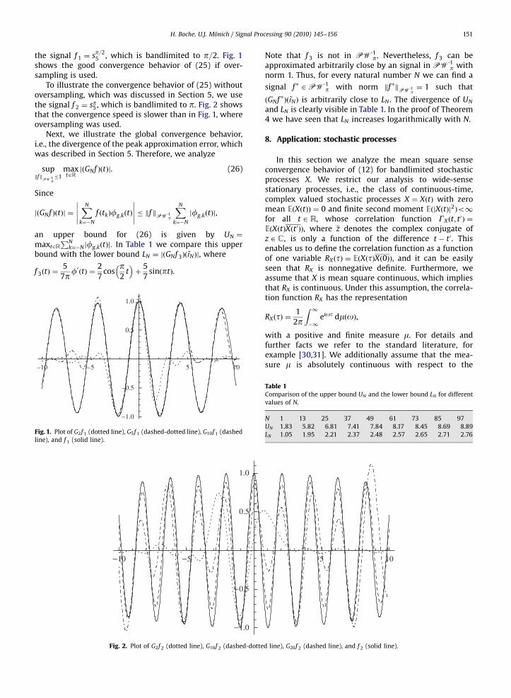
the signal f 1 ¼ sp=25 , which is bandlimited to p=2. Fig. 1

shows the good convergence behavior of (25) if over-sampling is used.

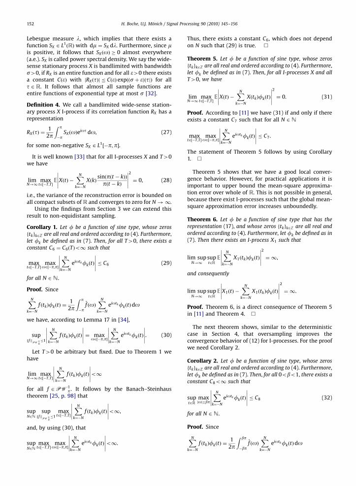
To illustrate the convergence behavior of (25) withoutoversampling, which was discussed in Section 5, we usethe signal f 2 ¼ sp5 , which is bandlimited to p. Fig. 2 showsthat the convergence speed is slower than in Fig. 1, whereoversampling was used.

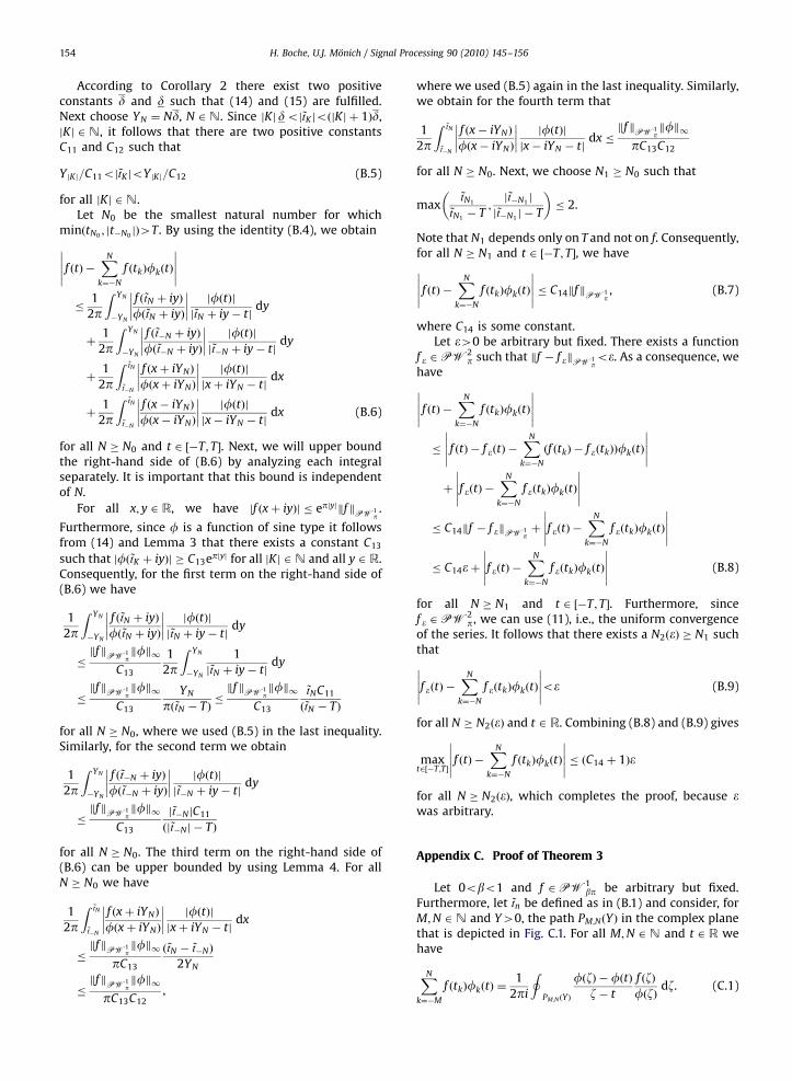
Next, we illustrate the global convergence behavior,i.e., the divergence of the peak approximation error, whichwas described in Section 5. Therefore, we analyze

supkfk

PW1p�1

maxt2RjðGNf ÞðtÞj. (26)

Since

jðGNf ÞðtÞj ¼XN

k¼�N

f ðtkÞfg;kðtÞ

���������� � kfkPW1

p

XN

k¼�N

jfg;kðtÞj,

an upper bound for (26) is given by UN ¼

maxt2R

PNk¼�N jfg;kðtÞj: In Table 1 we compare this upper

bound with the lower bound LN ¼ jðGNf 3ÞðtNÞj, where

f 3ðtÞ ¼5

7pf0ðtÞ ¼

2

7cos

p2

t� �

þ5

7sinðptÞ.

10 5 5 10

1.0

0.5

0.5

1.0

Fig. 1. Plot of G2f 1 (dotted line), G5f 1 (dashed-dotted line), G10f 1 (dashed

line), and f 1 (solid line).

0.5

1.0

10 5

1.0

0.5

Fig. 2. Plot of G2f 2 (dotted line), G10f 2 (dashed-dotte

Note that f 3 is not in PW1p. Nevertheless, f 3 can be

approximated arbitrarily close by an signal in PW1p with

norm 1. Thus, for every natural number N we can find a

signal f � 2 PW1p with norm kf �kPW1

p¼ 1 such that

ðGNf �ÞðtNÞ is arbitrarily close to LN . The divergence of UN

and LN is clearly visible in Table 1. In the proof of Theorem4 we have seen that LN increases logarithmically with N.

8. Application: stochastic processes

In this section we analyze the mean square senseconvergence behavior of (12) for bandlimited stochasticprocesses X. We restrict our analysis to wide-sensestationary processes, i.e., the class of continuous-time,complex valued stochastic processes X ¼ XðtÞ with zeromean EðXðtÞÞ ¼ 0 and finite second moment EðjXðtÞj2Þo1for all t 2 R, whose correlation function GXðt; t

0Þ ¼

EðXðtÞXðt0ÞÞ, where z denotes the complex conjugate ofz 2 C, is only a function of the difference t � t0. Thisenables us to define the correlation function as a functionof one variable RXðtÞ ¼ EðXðtÞXð0ÞÞ, and it can be easilyseen that RX is nonnegative definite. Furthermore, weassume that X is mean square continuous, which impliesthat RX is continuous. Under this assumption, the correla-tion function RX has the representation

RXðtÞ ¼1

2p

Z 1�1

eiot dmðoÞ,

with a positive and finite measure m. For details andfurther facts we refer to the standard literature, forexample [30,31]. We additionally assume that the mea-sure m is absolutely continuous with respect to the

5 10

d line), G20f 2 (dashed line), and f 2 (solid line).

Table 1Comparison of the upper bound UN and the lower bound LN for different

values of N.

N 1 13 25 37 49 61 73 85 97

UN 1.83 5.82 6.81 7.41 7.84 8.17 8.45 8.69 8.89

LN 1.05 1.95 2.21 2.37 2.48 2.57 2.65 2.71 2.76

ARTICLE IN PRESS

H. Boche, U.J. Monich / Signal Processing 90 (2010) 145–156152

Lebesgue measure l, which implies that there exists afunction SX 2 L1

ðRÞ with dm ¼ SX dl. Furthermore, since mis positive, it follows that SXðoÞ � 0 almost everywhere(a.e.). SX is called power spectral density. We say the wide-sense stationary process X is bandlimited with bandwidths40, if RX is an entire function and for all �40 there existsa constant Cð�Þ with jRXðtÞj � Cð�Þ expððsþ �ÞjtjÞ for allt 2 R. It follows that almost all sample functions areentire functions of exponential type at most s [32].

Definition 4. We call a bandlimited wide-sense station-ary process X I-process if its correlation function RX has arepresentation

RXðtÞ ¼1

2p

Z p

�pSXðoÞeiot do, (27)

for some non-negative SX 2 L1½�p;p�.

It is well known [33] that for all I-processes X and T40we have

limN!1

maxt2½�T ;T�

E XðtÞ �XN

k¼�N

XðkÞsinðpðt � kÞÞ

pðt � kÞ

����������2

¼ 0, (28)

i.e., the variance of the reconstruction error is bounded onall compact subsets of R and converges to zero for N!1.

Using the findings from Section 3 we can extend thisresult to non-equidistant sampling.

Corollary 1. Let f be a function of sine type, whose zeros

ftkgk2Z are all real and ordered according to (4). Furthermore,let fk be defined as in (7). Then, for all T40, there exists a

constant C6 ¼ C6ðTÞo1 such that

maxt2½�T ;T�

maxo2½�p;p�

XN

k¼�N

eiotkfkðtÞ

���������� � C6 (29)

for all N 2 N.

Proof. Since

XN

k¼�N

f ðtkÞfkðtÞ ¼1

2p

Z p

�pf ðoÞ

XN

k¼�N

eiotkfkðtÞdo

we have, according to Lemma 17 in [34],

supkfk

PW1p�1

XN

k¼�N

f ðtkÞfkðtÞ

���������� ¼ max

o2½�p;p�

XN

k¼�N

eiotkfkðtÞ

����������. (30)

Let T40 be arbitrary but fixed. Due to Theorem 1 wehave

limN!1

maxt2½�T ;T�

XN

k¼�N

f ðtkÞfkðtÞ

����������o1

for all f 2 PW1p. It follows by the Banach–Steinhaus

theorem [25, p. 98] that

supN2N

supkfk

PW1p�1

maxt2½�T ;T�

XN

k¼�N

f ðtkÞfkðtÞ

����������o1,

and, by using (30), that

supN2N

maxt2½�T;T�

maxo2½�p;p�

XN

k¼�N

eiotkfkðtÞ

����������o1.

Thus, there exists a constant C6, which does not dependon N such that (29) is true. &

Theorem 5. Let f be a function of sine type, whose zeros

ftkgk2Z are all real and ordered according to (4). Furthermore,let fk be defined as in (7). Then, for all I-processes X and all

T40, we have

limN!1

maxt2½�T ;T�

E XðtÞ �XN

k¼�N

XðtkÞfkðtÞ

����������2

¼ 0. (31)

Proof. According to [11] we have (31) if and only if thereexists a constant C7 such that for all N 2 N

maxt2½�T ;T�

maxo2½�p;p�

XN

k¼�N

eiotkfkðtÞ

���������� � C7.

The statement of Theorem 5 follows by using Corollary1. &

Theorem 5 shows that we have a good local conver-gence behavior. However, for practical applications it isimportant to upper bound the mean-square approxima-tion error over whole of R. This is not possible in general,because there exist I-processes such that the global mean-square approximation error increases unboundedly.

Theorem 6. Let f be a function of sine type that has the

representation (17), and whose zeros ftkgk2Z are all real and

ordered according to (4). Furthermore, let fk be defined as in

(7). Then there exists an I-process X1 such that

lim supN!1

supt2R

EXN

k¼�N

X1ðtkÞfkðtÞ

����������2

¼ 1,

and consequently

lim supN!1

supt2R

E X1ðtÞ �XN

k¼�N

X1ðtkÞfkðtÞ

����������2

¼ 1.

Proof. Theorem 6, is a direct consequence of Theorem 5in [11] and Theorem 4. &

The next theorem shows, similar to the deterministiccase in Section 4, that oversampling improves theconvergence behavior of (12) for I-processes. For the proofwe need Corollary 2.

Corollary 2. Let f be a function of sine type, whose zeros

ftkgk2Z are all real and ordered according to (4). Furthermore,let fk be defined as in (7). Then, for all 0obo1, there exists a

constant C8o1 such that

supt2R

maxjoj�bp

XN

k¼�N

eiotkfkðtÞ

���������� � C8 (32)

for all N 2 N.

Proof. Since

XN

k¼�N

f ðtkÞfkðtÞ ¼1

2p

Z bp

�bpf ðoÞ

XN

k¼�N

eiotkfkðtÞdo

ARTICLE IN PRESS

Fig. B.1. Path PNðYÞ in the complex plane.

H. Boche, U.J. Monich / Signal Processing 90 (2010) 145–156 153

we have, according to Lemma 17 in [34],

supkfk

PW1p�1

XN

k¼�N

f ðtkÞfkðtÞ

���������� ¼ max

joj�bp

XN

k¼�N

eiotkfkðtÞ

����������.

Using the Banach–Steinhaus theorem [25, p. 98] andTheorem 3, we obtain (32). &

Theorem 7. Let f be a function of sine type, whose zeros

ftkgk2Z are all real and ordered according to (4). Furthermore,let fk be defined as in (7). Then, for all 0obo1 and all

I-processes X, whose power spectral density SXðoÞ is

supported in ½�bp;bp�, we have

supN2N

supt2R

EXN

k¼�N

XðtkÞfkðtÞ

����������2

o1 (33)

and consequently

supN2N

supt2R

E XðtÞ �XN

k¼�N

XðtkÞfkðtÞ

����������2

o1.

Proof. According to [11] we have (33) if and only if thereexists a constant C9 such that for all N 2 N

supt2R

maxjoj�bp

XN

k¼�N

eiotkfkðtÞ

���������� � C9. (34)

The proof is complete because (34) is true byCorollary 2. &

Appendix A. Two lemmas

In this appendix we prove two lemmas, which areneeded for the proof of Theorems 1 and 3, given inAppendices B and C, respectively.

Lemma 4. Let f be a function of sine type, whose zeros are

all real, and Y040. Then there exists a constant C10 such

that, for all 0ob � 1, jYj � Y0, A;B 2 R, A � B, t 2 R, and

f 2 PW1bp, we have

Z B

A

f ðxþ iYÞ

fðxþ iYÞ

fðtÞxþ iY � t

��������dx �

ðB� AÞkfkPW1bpkfk1

C10jY j.

Proof of Lemma 4. For all x;Y 2 R, we havejf ðxþ iYÞj � ebpjYjkfkPW1

bp. Furthermore, since f is a func-

tion of sine type with all zeros being real, it follows fromLemma 3 that there exists a constant C10 such that jfðxþiYÞj � C10epjYj for all x 2 R and all jYj � Y0. Therefore, weobtain

Z B

A

f ðxþ iYÞ

fðxþ iYÞ

fðtÞxþ iY � t

��������dx �

kfkPW1bpkfk1

C10

Z B

A

e�pð1�bÞjYj

jxþ iY � tjdx

�

ðB� AÞkfkPW1bpkfk1

C10jYj,

which completes the proof. &

For the proof of Theorem 3 we need the followinglemma.

Lemma 5. Let f be a function of sine type, whose zeros

ftkgk2Z are all real and ordered according to (4), 0obo1,

and tn as defined in (B.1). Then there exist a constant C10

such that for all jKj 2N, Y40, t 2 R with jt � tK j � d, and

f 2 PW1bp we have

Z Y

�Y

f ðtK þ iyÞ

fðtK þ iyÞ

fðtÞtK þ iy� t

��������dy �

2kfkPW1bpkfk1

pC10 dð1� bÞ.

Proof of Lemma 5. For all x; y 2 R, we havejf ðxþ iyÞj � ebpjyjkfkPW1

bp. Furthermore, since f is a func-

tion of sine type it follows from Lemma 3 and (14) thatthere exists a constant C10 such that jfðtK þ iyÞj � C10epjyj

for all jKj 2 N and y 2 R. Therefore, we obtainZ Y

�Y

f ðtN þ iyÞ

fðtN þ iyÞ

fðtÞtN þ iy� t

��������dy

�

kfkPW1bpkfk1

C10

Z Y

�Y

e�pð1�bÞjyj

tN þ iy� t

��������dy

�

2kfkPW1bpkfk1

C10 d

Z Y

0e�pð1�bÞy dy �

2kfkPW1bpkfk1

pC10 dð1� bÞ,

which completes the proof. &

Appendix B. Proof of Theorem 1

Let T40 and f 2 PW1p be arbitrary but fixed and

tn ¼ðtnþ1 þ tnÞ=2 for n � 1;

ðtn�1 þ tnÞ=2 for n � �1:

((B.1)

Furthermore, consider, for N 2N and Y40, the path PNðYÞ

in the complex plane that is depicted in Fig. B.1. For allN 2 N and t 2 R we have the equality

XN

k¼�N

f ðtkÞfkðtÞ ¼1

2pi

IPN ðYÞ

fðzÞ �fðtÞz� t

f ðzÞfðzÞ

dz. (B.2)

Eq. (B.2) can be easily seen by using the method ofresidues. Note that by the choice of PNðYÞ we have fðzÞa0for all z 2 PNðYÞ. Furthermore, for all N 2 N and t 2 R witht�NototN , we have

1

2pi

IPN ðYÞ

fðzÞ � fðtÞz� t

f ðzÞfðzÞ

dz

¼1

2pi

IPN ðYÞ

f ðzÞz� t

dz�1

2pi

IPN ðYÞ

fðtÞz� t

f ðzÞfðzÞ

dz

¼ f ðtÞ �1

2pi

IPN ðYÞ

fðtÞz� t

f ðzÞfðzÞ

dz. (B.3)

Combining (B.2) and (B.3), it follows that

f ðtÞ �XN

k¼�N

f ðtkÞfkðtÞ ¼1

2pi

IPN ðYÞ

fðtÞz� t

f ðzÞfðzÞ

dz (B.4)

for all N 2 N and t 2 R with t�NototN .

ARTICLE IN PRESS

H. Boche, U.J. Monich / Signal Processing 90 (2010) 145–156154

According to Corollary 2 there exist two positiveconstants d and d such that (14) and (15) are fulfilled.Next choose YN ¼ Nd, N 2 N. Since jKjdojtK joðjKj þ 1Þd,jKj 2 N, it follows that there are two positive constantsC11 and C12 such that

Y jKj=C11ojtK joY jKj=C12 (B.5)

for all jKj 2 N.Let N0 be the smallest natural number for which

minðtN0; jt�N0

jÞ4T . By using the identity (B.4), we obtain

f ðtÞ �XN

k¼�N

f ðtkÞfkðtÞ

����������

�1

2p

Z YN

�YN

f ðtN þ iyÞ

fðtN þ iyÞ

�������� jfðtÞjjtN þ iy� tj

dy

þ1

2p

Z YN

�YN

f ðt�N þ iyÞ

fðt�N þ iyÞ

�������� jfðtÞjjt�N þ iy� tj

dy

þ1

2p

Z tN

t�N

f ðxþ iYNÞ

fðxþ iYNÞ

�������� jfðtÞjjxþ iYN � tj

dx

þ1

2p

Z tN

t�N

f ðx� iYNÞ

fðx� iYNÞ

�������� jfðtÞjjx� iYN � tj

dx (B.6)

for all N � N0 and t 2 ½�T; T�. Next, we will upper boundthe right-hand side of (B.6) by analyzing each integralseparately. It is important that this bound is independentof N.

For all x; y 2 R, we have jf ðxþ iyÞj � epjyjkfkPW1p.

Furthermore, since f is a function of sine type it followsfrom (14) and Lemma 3 that there exists a constant C13

such that jfðtK þ iyÞj � C13epjyj for all jKj 2 N and all y 2 R.Consequently, for the first term on the right-hand side of(B.6) we have

1

2p

Z YN

�YN

f ðtN þ iyÞ

fðtN þ iyÞ

�������� jfðtÞjjtN þ iy� tj

dy

�kfkPW1

pkfk1

C13

1

2p

Z YN

�YN

1

jtN þ iy� tjdy

�kfkPW1

pkfk1

C13

YN

pðtN � TÞ�kfkPW1

pkfk1

C13

tNC11

ðtN � TÞ

for all N � N0, where we used (B.5) in the last inequality.Similarly, for the second term we obtain

1

2p

Z YN

�YN

f ðt�N þ iyÞ

fðt�N þ iyÞ

�������� jfðtÞjjt�N þ iy� tj

dy

�kfkPW1

pkfk1

C13

jt�NjC11

ðjt�Nj � TÞ

for all N � N0. The third term on the right-hand side of(B.6) can be upper bounded by using Lemma 4. For allN � N0 we have

1

2p

Z tN

t�N

f ðxþ iYNÞ

fðxþ iYNÞ

�������� jfðtÞjjxþ iYN � tj

dx

�kfkPW1

pkfk1

pC13

ðtN � t�NÞ

2YN

�kfkPW1

pkfk1

pC13C12,

where we used (B.5) again in the last inequality. Similarly,we obtain for the fourth term that

1

2p

Z tN

t�N

f ðx� iYNÞ

fðx� iYNÞ

�������� jfðtÞjjx� iYN � tj

dx �kfkPW1

pkfk1

pC13C12

for all N � N0. Next, we choose N1 � N0 such that

maxtN1

tN1� T

;jt�N1j

jt�N1j � T

� �� 2.

Note that N1 depends only on T and not on f. Consequently,for all N � N1 and t 2 ½�T; T�, we have

f ðtÞ �XN

k¼�N

f ðtkÞfkðtÞ

���������� � C14kfkPW1

p, (B.7)

where C14 is some constant.Let �40 be arbitrary but fixed. There exists a function

f � 2 PW2p such that kf � f �kPW1

po�. As a consequence, we

have

f ðtÞ �XN

k¼�N

f ðtkÞfkðtÞ

����������

� f ðtÞ � f �ðtÞ �XN

k¼�N

ðf ðtkÞ � f �ðtkÞÞfkðtÞ

����������

þ f �ðtÞ �XN

k¼�N

f �ðtkÞfkðtÞ

����������

� C14kf � f �kPW1pþ f �ðtÞ �

XN

k¼�N

f �ðtkÞfkðtÞ

����������

� C14�þ f �ðtÞ �XN

k¼�N

f �ðtkÞfkðtÞ

���������� (B.8)

for all N � N1 and t 2 ½�T; T�. Furthermore, sincef � 2 PW2

p, we can use (11), i.e., the uniform convergenceof the series. It follows that there exists a N2ð�Þ � N1 suchthat

f �ðtÞ �XN

k¼�N

f �ðtkÞfkðtÞ

����������o� (B.9)

for all N � N2ð�Þ and t 2 R. Combining (B.8) and (B.9) gives

maxt2½�T ;T�

f ðtÞ �XN

k¼�N

f ðtkÞfkðtÞ

���������� � C14 þ 1ð Þ�

for all N � N2ð�Þ, which completes the proof, because �was arbitrary.

Appendix C. Proof of Theorem 3

Let 0obo1 and f 2 PW1bp be arbitrary but fixed.

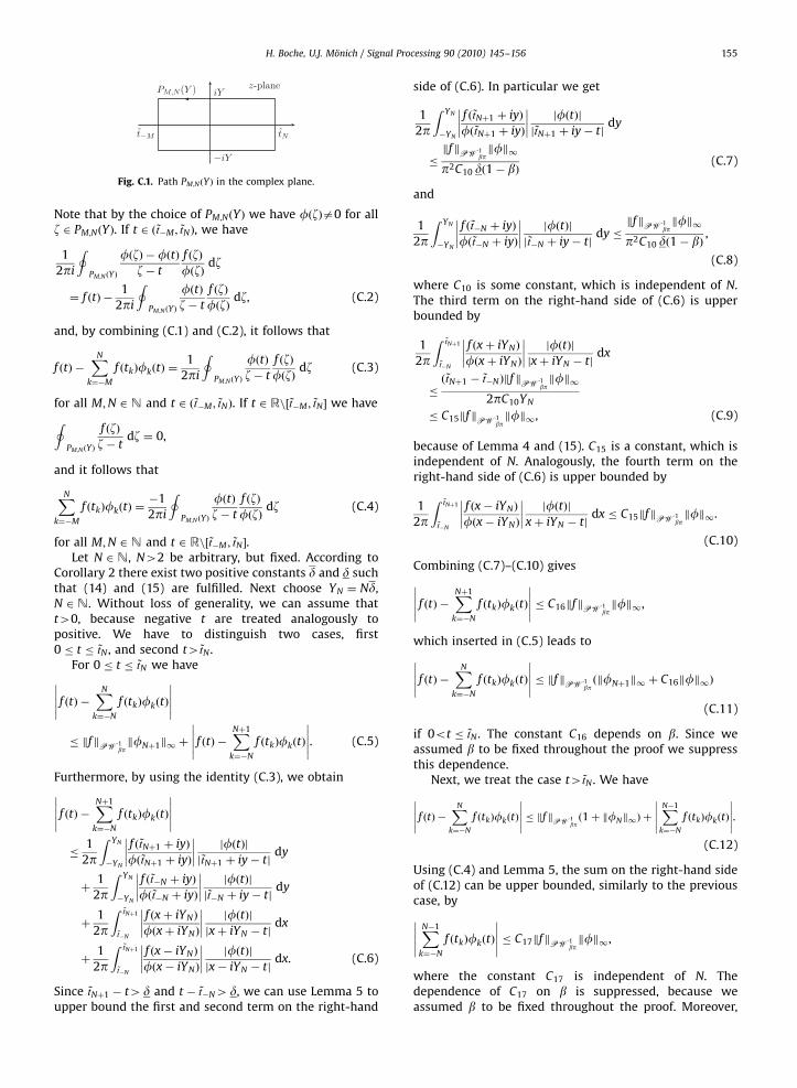
Furthermore, let tn be defined as in (B.1) and consider, forM;N 2 N and Y40, the path PM;NðYÞ in the complex planethat is depicted in Fig. C.1. For all M;N 2 N and t 2 R wehave

XN

k¼�M

f ðtkÞfkðtÞ ¼1

2pi

IPM;N ðYÞ

fðzÞ � fðtÞz� t

f ðzÞfðzÞ

dz. (C.1)

ARTICLE IN PRESS

Fig. C.1. Path PM;NðYÞ in the complex plane.

H. Boche, U.J. Monich / Signal Processing 90 (2010) 145–156 155

Note that by the choice of PM;NðYÞ we have fðzÞa0 for allz 2 PM;NðYÞ. If t 2 ðt�M ; tNÞ, we have

1

2pi

IPM;N ðYÞ

fðzÞ �fðtÞz� t

f ðzÞfðzÞ

dz

¼ f ðtÞ �1

2pi

IPM;N ðYÞ

fðtÞz� t

f ðzÞfðzÞ

dz, (C.2)

and, by combining (C.1) and (C.2), it follows that

f ðtÞ �XN

k¼�M

f ðtkÞfkðtÞ ¼1

2pi

IPM;N ðYÞ

fðtÞz� t

f ðzÞfðzÞ

dz (C.3)

for all M;N 2 N and t 2 ðt�M ; tNÞ. If t 2 Rn½t�M ; tN� we haveIPM;N ðYÞ

f ðzÞz� t

dz ¼ 0,

and it follows that

XN

k¼�M

f ðtkÞfkðtÞ ¼�1

2pi

IPM;N ðYÞ

fðtÞz� t

f ðzÞfðzÞ

dz (C.4)

for all M;N 2 N and t 2 Rn½t�M ; tN�.Let N 2 N, N42 be arbitrary, but fixed. According to

Corollary 2 there exist two positive constants d and d suchthat (14) and (15) are fulfilled. Next choose YN ¼ Nd,N 2 N. Without loss of generality, we can assume thatt40, because negative t are treated analogously topositive. We have to distinguish two cases, first0 � t � tN , and second t4tN .

For 0 � t � tN we have

f ðtÞ �XN

k¼�N

f ðtkÞfkðtÞ

����������

� kfkPW1bpkfNþ1k1 þ f ðtÞ �

XNþ1

k¼�N

f ðtkÞfkðtÞ

����������. (C.5)

Furthermore, by using the identity (C.3), we obtain

f ðtÞ �XNþ1

k¼�N

f ðtkÞfkðtÞ

����������

�1

2p

Z YN

�YN

f ðtNþ1 þ iyÞ

fðtNþ1 þ iyÞ

�������� jfðtÞjjtNþ1 þ iy� tj

dy

þ1

2p

Z YN

�YN

f ðt�N þ iyÞ

fðt�N þ iyÞ

�������� jfðtÞjjt�N þ iy� tj

dy

þ1

2p

Z tNþ1

t�N

f ðxþ iYNÞ

fðxþ iYNÞ

�������� jfðtÞjjxþ iYN � tj

dx

þ1

2p

Z tNþ1

t�N

f ðx� iYNÞ

fðx� iYNÞ

�������� jfðtÞjjx� iYN � tj

dx. (C.6)

Since tNþ1 � t4d and t � t�N4 d, we can use Lemma 5 toupper bound the first and second term on the right-hand

side of (C.6). In particular we get

1

2p

Z YN

�YN

f ðtNþ1 þ iyÞ

fðtNþ1 þ iyÞ

�������� jfðtÞjjtNþ1 þ iy� tj

dy

�

kfkPW1bpkfk1

p2C10 dð1� bÞ(C.7)

and

1

2p

Z YN

�YN

f ðt�N þ iyÞ

fðt�N þ iyÞ

�������� jfðtÞjjt�N þ iy� tj

dy �kfkPW1

bpkfk1

p2C10 dð1� bÞ,

(C.8)

where C10 is some constant, which is independent of N.The third term on the right-hand side of (C.6) is upperbounded by

1

2p

Z tNþ1

t�N

f ðxþ iYNÞ

fðxþ iYNÞ

�������� jfðtÞjjxþ iYN � tj

dx

�

ðtNþ1 � t�NÞkfkPW1bpkfk1

2pC10YN

� C15kfkPW1bpkfk1, (C.9)

because of Lemma 4 and (15). C15 is a constant, which isindependent of N. Analogously, the fourth term on theright-hand side of (C.6) is upper bounded by

1

2p

Z tNþ1

t�N

f ðx� iYNÞ

fðx� iYNÞ

�������� jfðtÞjxþ iYN � tj

dx � C15kfkPW1bpkfk1.

(C.10)

Combining (C.7)–(C.10) gives

f ðtÞ �XNþ1

k¼�N

f ðtkÞfkðtÞ

���������� � C16kfkPW1

bpkfk1,

which inserted in (C.5) leads to

f ðtÞ �XN

k¼�N

f ðtkÞfkðtÞ

���������� � kfkPW1

bpðkfNþ1k1 þ C16kfk1Þ

(C.11)

if 0ot � tN . The constant C16 depends on b. Since weassumed b to be fixed throughout the proof we suppressthis dependence.

Next, we treat the case t4tN . We have

f ðtÞ �XN

k¼�N

f ðtkÞfkðtÞ

���������� � kf kPW1

bpð1þ kfNk1Þ þ

XN�1

k¼�N

f ðtkÞfkðtÞ

����������.

(C.12)

Using (C.4) and Lemma 5, the sum on the right-hand sideof (C.12) can be upper bounded, similarly to the previouscase, by

XN�1

k¼�N

f ðtkÞfkðtÞ

���������� � C17kfkPW1

bpkfk1,

where the constant C17 is independent of N. Thedependence of C17 on b is suppressed, because weassumed b to be fixed throughout the proof. Moreover,

ARTICLE IN PRESS

H. Boche, U.J. Monich / Signal Processing 90 (2010) 145–156156

by (C.12), we finally obtain

f ðtÞ �XN

k¼�N

f ðtkÞfkðtÞ

���������� � kfkPW1

bpð1þ kfNk1 þ C17kfk1Þ.

(C.13)

if t4tN .

From (C.11) and (C.13) we see that jf ðtÞ �PNk¼�Nf ðtkÞfkðtÞj � kfkPW1

bpC18 for all t40, with some

constant C18 that is independent of t and N. Since N42was arbitrary and the same upper bound holds fornegative t, it follows that

maxt2R

f ðtÞ �XN

k¼�N

f ðtkÞfkðtÞ

���������� � kfkPW1

bpC18 (C.14)

for all N42.Finally, using the same arguments as in the proof of

Theorem 1 we obtain limN!1maxt2Rjf ðtÞ�PN

k¼�Nf ðtkÞ

fkðtÞj ¼ 0, which completes the proof.

For the proof it was important to find (C.14), i.e., anupper bound that is independent of t. A closer look at theproof of Theorem 3 reveals that oversampling, i.e., bo1, isessential for the approach that was used to obtain (C.14).The same approach cannot be used for b! 1, because theright-hand sides of (C.7) and (C.8) diverge.

References

[1] H. Boche, U.J. Monich, Local and global convergence behavior ofnon-equidistant sampling series, in: IEEE International Conferenceon Acoustics, Speech, and Signal Processing (ICASSP ’09), 2009,pp. 2945–2948.

[2] K. Yao, J.B. Thomas, On some stability and interpolatory propertiesof nonuniform sampling expansions, IEEE Transactions on Circuitsand Systems 14 (4) (1967) 404–408.

[3] H.J. Landau, Sampling, data transmission, and the Nyquist rate,Proceedings of the IEEE 55 (10) (1967) 1701–1706.

[4] J.R. Higgins, A sampling theorem for irregularly spaced samplepoints, IEEE Transactions on Information Theory 22 (5) (1976)621–622.

[5] M.M. Milosavljevic, M.R. Dostanic, On generalized stable nonuni-form sampling expansions involving derivatives, IEEE Transactionson Information Theory 43 (5) (1997) 1714–1716.

[6] K.M. Flornes, Y. Lyubarskii, K. Seip, A direct interpolation method forirregular sampling, Applied and Computational Harmonic Analysis7 (3) (1999) 305–314.

[7] H.G. Feichtinger, K. Grochenig, Theory and practice of irregularsampling, in: Wavelets: Mathematics and Applications, Studies inAdvanced Mathematics, CRC, Boca Raton, FL, 1994, pp. 305–363.

[8] K. Grochenig, Irregular sampling, Toeplitz matrices, and theapproximation of entire functions of exponential type, Mathematicsof Computation 68 (226) (1999) 749–765.

[9] K. Seip, An irregular sampling theorem for functions bandlimited ina generalized sense, SIAM Journal on Applied Mathematics 47 (5)(1987) 1112–1116.

[10] G. Hinsen, Irregular sampling of bandlimited Lp-functions, Journalof Approximation Theory 72 (3) (1993) 346–364.

[11] H. Boche, U.J. Monich, Non-uniform sampling—signal and systemrepresentation, in: Proceedings of the 2008 International Sympo-sium on Information Theory and its Applications (ISITA2008), 2008,pp. 1576–1581.

[12] B. Lacaze, Reconstruction formula for irregular sampling, SamplingTheory in Signal and Image Processing 4 (1) (2005) 33–43.

[13] C. Houdre, Reconstruction of band limited processes from irregularsamples, The Annals of Probability 23 (2) (1995) 674–696.

[14] F. Marvasti (Ed.), Nonuniform Sampling: Theory and Practice,Kluwer Academic/Plenum Publishers, 2001.

[15] B.Y. Levin, Lectures on Entire Functions, AMS, 1996.[16] R.M. Young, An Introduction to Nonharmonic Fourier Series,

Academic Press, New York, 1980.[17] B.J. Levin, I.V. Ostrovskii, On small perturbations of the set of zeros

of functions of sine type, Mathematics of the USSR Izvestiya 14 (43)(1980) 79–101.

[18] A.E. Eremenko, M.L. Sodin, Parametrization of entire functions ofsine-type by their critical values, Advances in Soviet Mathematics11 (1992) 238–242.

[19] J.L. Brown Jr., On the error in reconstructing a non-band-limited function by means of the bandpass sampling theorem,Journal of Mathematical Analysis and Applications 18 (1967) 75–84Erratum, Journal of Mathematical Analysis and Applications 21(1968) 699.

[20] P.L. Butzer, W. Splettstoßer, R.L. Stens, The sampling theorem andlinear prediction in signal analysis, Jahresbericht der DeutschenMathematiker-Vereiningung 90 (1) (1988) 1–70.

[21] P.L. Butzer, R.L. Stens, Sampling theory for not necessarily band-limited functions: a historical overview, SIAM Review 34 (1) (1992)40–53.

[22] H. Boche, U.J. Monich, On stable Shannon type reconstructionprocesses, Signal Processing 88 (6) (2008) 1477–1484.

[23] H. Boche, U.J. Monich, Global and local approximation behavior ofreconstruction processes for Paley–Wiener functions, SamplingTheory in Signal and Image Processing 8 (1) (2009) 23–51.

[24] H. Boche, U.J. Monich, There exists no globally uniformly con-vergent reconstruction for the Paley–Wiener space PW1

p ofbandlimited functions sampled at Nyquist rate, IEEE Transactionson Signal Processing 56 (7) (2008) 3170–3179.

[25] W. Rudin, Real and Complex Analysis, third ed., McGraw-Hill, NewYork, 1987.

[26] I. Bar-David, An implicit sampling theorem for boundedbandlimited functions, Information and Control 24 (1) (1974)36–44.

[27] E. Masry, S. Cambanis, Consistent estimation of continuous-timesignals from nonlinear transformations of noisy samples, IEEETransactions on Information Theory 27 (1) (1981) 84–96.

[28] B.F. Logan Jr., Signals designed for recovery after clipping—I.Localization of infinite products, AT&T Bell Laboratories TechnicalJournal 63 (2) (1984) 261–285.

[29] R. Duffin, A.C. Schaeffer, Some properties of functions of exponen-tial type, Bulletin of the American Mathematical Society 44 (4)(1938) 236–240.

[30] M. Loeve, Probability Theory, third ed., Van Nostrand, Princeton, NJ,1963.

[31] H. Cramer, M.R. Leadbetter, Stationary and Related StochasticProcesses, Dover Publications, New York, 2004.

[32] Y.K. Belyaev, Analytic random processes, Theory of Probability andits Applications 4 (4) (1959) 402–409.

[33] J.L. Brown Jr., Truncation error for band-limited random processes,Information Sciences 1 (1969) 171–261.

[34] H. Boche, U.J. Monich, Limits of signal processing performanceunder thresholding, Signal Processing 89 (8) (2009) 1634–1646.