Shadow banking and the dynamics of aggregate leverage: An application of the Kalman filter to...
53
Cahier de recherche 2011-01 Shadow banking and leverage: An application of the Kalman filter to time-varying cyclical leverage measures† Système bancaire parallèle et levier : Une application du filtre de Kalman aux mesures dynamiques du levier Christian Calmès a,* , Raymond Théoret b a Chaire d’information financière et organisationnelle, ESG-UQAM; Laboratory for Research in Statistics and Probability, LRSP; Université du Québec (Outaouais), Pavillon Lucien-Brault, 101 rue Saint-Jean-Bosco, Gatineau, Québec, Canada. b Université du Québec (Montréal), École des sciences de la gestion, 315 est Ste-Catherine, Montréal, Québec, Canada ; Professeur associé, Université du Québec (Outaouais); Chaire d’information financière et organisationnelle, ESG-UQAM. This version: January 14 th , 2011 ___________________________________________________________________ * Corresponding author. Tel: +1 819 595 3000 1893; fax: +1 819 773 1747 E-mail addresses: [email protected] (C. Calmès), [email protected] (R. Théoret). † We thank Céline Gauthier and Étienne Bordeleau, economists at the Bank of Canada, for their helpful suggestions, and for the data they provided to us. We also thank Alain Angola for his research assistance.
Transcript of Shadow banking and the dynamics of aggregate leverage: An application of the Kalman filter to...
Cahier de recherche
2011-01
Shadow banking and leverage: An application of the Kalman filter to time-varying cyclical leverage measures†
Système bancaire parallèle et levier : Une application du filtre de Kalman aux mesures dynamiques du levier Christian Calmèsa,*, Raymond Théoretb
a Chaire d’information financière et organisationnelle, ESG-UQAM; Laboratory for Research in Statistics and Probability, LRSP; Université du Québec (Outaouais), Pavillon Lucien-Brault, 101 rue Saint-Jean-Bosco, Gatineau, Québec, Canada. b Université du Québec (Montréal), École des sciences de la gestion, 315 est Ste-Catherine, Montréal, Québec, Canada ; Professeur associé, Université du Québec (Outaouais); Chaire d’information financière et organisationnelle, ESG-UQAM.
This version: January 14th , 2011
___________________________________________________________________ * Corresponding author. Tel: +1 819 595 3000 1893; fax: +1 819 773 1747 E-mail addresses: [email protected] (C. Calmès), [email protected] (R. Théoret). † We thank Céline Gauthier and Étienne Bordeleau, economists at the Bank of Canada, for their helpful suggestions, and for the data they provided to us. We also thank Alain Angola for his research assistance.
© Christian Calmès and Raymond Théoret.
2
Shadow banking and leverage: An application of the Kalman filter to time-varying cyclical leverage measures
Abstract
During the last decades, banks off-balance sheet (OBS) activities (e.g. securitization, trading and fee-based activities) have greatly contributed to the increase in bank risk. However, the standard financial indicators such as the Value-at-Risk and the accounting leverage, exclude these non-traditional activities, and neglect the increased risk market-oriented banking generates. In this paper, we study various measures of leverage incorporating the risks associated to this new type of banking activities (i.e. “shadow banking”) in a dynamic setting, relying on Kalman filtering procedure and different detrending methods. Applying this framework to Canadian data, we can detect the increase in banking riskiness years before what the conventional risk measures predict. We also find that the elasticity measures of leverage, compared to the simple balance sheet ratios like the ratio of assets to equity, are generally more forward-looking indicators of bank risk, and better capture the cyclical pattern of bank leverage. In particular, it appears that OBS activities exert a stronger influence on these leverage measures during expansion periods.
Keywords: Leverage, Banking, Off-balance sheet activities, Liquidity, Kalman Filter. JEL classification: C13, C22, C51, G21, G32.
Système bancaire parallèle et levier : Une application du filtre de Kalman aux mesures dynamiques de levier
Résumé Au cours des dernières décennies, les activités hors-bilan des banques (i.e. titrisation, activités de négociation et services bancaires) ont grandement contribué à l’accroissement du risque bancaire. Cependant, les indicateurs financiers conventionnels, tels que la valeur à risque et le levier comptable, excluent ces activités non traditionnelles et négligent le risque accru que génèrent les activités bancaires orientées vers les marchés financiers. Dans ce papier, nous étudions différentes mesures de levier qui incorporent les risques reliés au système bancaire parallèle dans un contexte dynamique fondé sur la procédure du filtre de Kalman et sur différentes méthodes de redressement. En transposant ce cadre d’analyse aux données canadiennes, nous pouvons déceler l’accroissement du risque bancaire bien avant les mesures conventionnelles du risque. Nous trouvons aussi que les mesures de levier formulées en termes d’élasticités sont de meilleurs indicateurs prévisionnels du risque bancaire que des mesures simplistes tel le ratio des actifs à l’équité. Elles captent également mieux le profil cyclique du levier. En particulier, les activités hors-bilan exercent un impact important sur ces mesures du levier durant les périodes de reprise économique. Mots-clefs : Levier, banques, activités hors-bilan, liquidité, filtre de Kalman. Classification JEL: C13, C22, C51, G21, G32.
© Christian Calmès and Raymond Théoret.
3
1. Introduction
Since banks have been allowed to conduct new types of off-balance-sheet (OBS)
activities, e.g., non-traditional activities such as underwriting and securitization, their
financial flows have become more volatile. For example, in Canada, before the mid
1990s, the volatility of stock trading portfolio was moderate, but following the emergence
of the market-oriented banking (i.e., “shadow banking”, Shin 2009), as banks got more
involved in OBS activities, this volatility exploded with the growing share of stocks in
assets (Figure 1). The same pattern emerges if we look at mortgages and consumer credit
originated by banks, the type of assets banks increasingly securitize, i.e. transfer off their
balance sheet (respectively Figures 2 and 3). As a matter of fact, most categories of banks
assets and liabilities share the same pattern and display a marked change in financial
flows volatilities. The associated increase in bank earnings volatility is generally
attributed to the fact that the volatility of OBS activities is greater than the volatility of
the traditional banking activities (Stiroh 2004, 2006a; Stiroh and Rumble 2006; Calmès
and Théoret 2009, 2010). There is also evidence that the higher risk-taking associated to
shadow banking results in greater levels of total leverage, i.e., both operating and
financial (DeYoung and Roland 2001, Shin 2009, Adrian and Shin 2010).
Insert Figure 1 about here
Leverage is a key indicator of bank risk (Hamada 1972, Rhee 1986, Griffin and
Dungan 2003, and Cihak and Schaeck, 2007, Stein 2010), but, unfortunately, the
traditional measures of leverage used to monitor bank risk usually fail to capture the
contribution of banks OBS activities to systemic risk. In practice, the standard leverage
measures are often based on simple ratios computed using balance sheet data, like the
© Christian Calmès and Raymond Théoret.
4
ratio of assets or risk-weighted assets to equity, or the ratio of debt to equity. Due to their
accounting flavour, these measures are rarely forward-looking, and may even be
sometimes misleading. For instance, in its June 2009 Financial System Review, the Bank
of Canada states that the increase in the spread between observed leverages, including
and excluding securization, is not worrying because securitized assets represent “only”
10% of Canadian banks balance-sheet assets, and concludes that “leverage was relatively
stable during the years leading to the financial crisis”. However, different conclusions
could be reached if, despite their low weight, some OBS activities impact on bank risk
was substantial. For example, the relative weight of the trading portfolio as a share of
banks non-traditional activities may be low, but trading is an important driver of banks
noninterest income1 volatility, which, in turn, feeds into the volatility of banks returns
(Stiroh 2006b, Stiroh and Rumble 2006, Calmès and Théoret 2009, Calmès and Liu 2009,
Calmès and Théoret 2010).
In this respect, it appears rather hazardous to rely on the classical measures of
leverage to directly assess the risk stemming from shadow banking. More sophisticated
bank risk analyses based on Z-scores or Tobin's q often deliver contradictory results
however. For example, in his international study on bank risk, Ratnovski (2009)
concludes that Canadian banking systemic risk is relatively low on the basis of
conventional capital ratios2. Using a Black-Scholes framework to price Canadian banks
franchises, Liu et al. (2006) arrive at a similar conclusion, but their approach may
underestimate bank risk, since assuming a Gaussian distribution of returns neglects fat-
tails risk, precisely the kind of risk inherent to derivatives found in OBS activities. In 1 Noninterest income is income banks generate off-balance sheet. 2 Another factor invoked by Ratnovski (2009) to account for the relatively low risk in the Canadian banking system relates to the Canadian banks funding structure. Canadian banks use a greater proportion of retail deposits to fund their operations than the international representative bank, which contributes to decrease their risk exposure.
© Christian Calmès and Raymond Théoret.
5
another study, comparing the Z-scores of different banking systems, Rajan (2005) is not
so positive about the Canadian banking system resilience. He actually finds that financial
deepening and higher regulatory capital ratios have not made Canadian banks safer.
Insert Figures 2 and 3 about here
The primary goal of this paper is to show that conventional measures of bank
leverage are actually not suited to gauge bank risk because they fail to directly account
for the risk associated to OBS activities. The task of searching for relevant measures of
bank leverage – i.e., effective leverage, including the risk associated to OBS activities –
was first undertaken by Breuer (2002). The author proposes an off-balance-sheet leverage
measure based on the Black and Scholes formula and finds that, compared to this
measure, the conventional measures of leverage indeed underestimate banks true
leverage. In the same vein, DeYoung and Roland (2001) analyze the average banks total
leverage, and find that market-oriented activities such as fee-based activities and trading
activities contribute substantially to banks total leverage. The detrending method they use
to compute the elasticity of earnings to revenue, i.e. their measure of total leverage, is
based on a cubic trend. By contrast, in this study, we rely on several detrending
techniques, including first-differences, logarithmic and HP filtering. In addition,
compared to DeYoung and Roland (2001) and Breuer (2002), we are not concerned by
one particular leverage measure, but rather document the relative performance of a
number of alternative measures of aggregate bank leverage to challenge the traditional
measures generally followed in bank risk monitoring. For example, only few studies
consider the role played by liquidity on banks leveraging, even though, considering the
most recent literature on banking leverage, and especially in the context of shadow
© Christian Calmès and Raymond Théoret.
6
banking, it is clear that liquidity has an important role to play in the banks leveraging
process (Farhi and Tirole 2009, Shin 2009). Indeed, short-term liquidity, considered as
negative debt, is used by financial institutions to pile up short-term liquid assets when the
degree of standard leverage passes a certain threshold. Banks rely on securitization to
generate new cash, which facilitates regulatory capital arbitrage (RCA, Brunnermeier
2010). This phenomenon is likely to be better detected in countries imposing stringent
capital requirements. Actually, one of the main advantages of analyzing Canadian data is
that Canadian banks are subjected to both a risk-weighted capital requirement and a
capital ceiling. Hence, if liquidity plays any role in terms of RCA and shows up in
Canadian data, despite the fact that Canada is believed to be less involved in shadow
banking, the associated leverage measures we develop could also deliver significant
results when applied to other datasets.
In this paper, we compare the relative performance of various leverage measures
proposed in previous studies and develop new ones, considering different dimensions of
leverage in the presence of OBS risk, like the connection between liquidity and leverage,
in a framework designed to account for the forward-looking nature of a desirable measure
of bank risk, and we also examine the issue of detrending, and the cyclicality of leverage.
More precisely, we define different measures of leverage, the degree of total leverage, the
elasticities of net value to assets, equity to assets, earnings to interest and noninterest
income, and noninterest income to interest income. We analyze these various leverage
measures in a dynamic setting bearing in mind the cyclical nature of leverage, and rely on
Kalman filtering to account for the procyclicality of bank leverage, discussed in Shin
(2009). As the dual of a dynamic programming problem (Ljungqvist and Sargent 2004),
© Christian Calmès and Raymond Théoret.
7
the Kalman filter allows the computation of an optimal leverage cycle, conditional on all
the information available at the time of computation3. In the same vein, we also study the
impact of the detrending method on the behaviour of the leverage cycle. Since most of
the series used to compute leverage are non-stationary, we begin by detrending them
resorting to first-differences, an obvious method, yet rarely considered in the leverage
literature. Various detrending methods can sometime deliver contradictory results
(Canova 1998), and the detrending method used to compute leverage may have a
significant impact on the dynamic behaviour of leverage obtained by Kalman filtering.
For this reason we also consider log-detrending (O’Brien and Vanderheiden 1987), cubic
detrending, with or without log residuals (DeYoung and Roland 2001), and Hodrick-
Prescott detrending. Our results suggest that the cubic detrending method of DeYoung
and Roland (2001), which neglects logarithms to compute residuals, does not deliver very
conclusive results in our setting. By comparison, we find that the log-detrending method
and the Hodrick-Prescott filter provide more consistent results, regardless of the leverage
measure considered.
In this framework, the series of experiments we run suggest that traditional
leverage measures based on balance-sheet data are not particularly suited to capture the
true behaviour of bank risk, and not so much because they are time-invariant, but because
they tend to exclude the new role played by OBS activities. For example, because of the
regulatory constraints imposed on capital, banks display a fairly constant target levels for
their conventional leverage measures. Indeed, the most followed measure of bank
leverage displays a flat plot during the years preceding the subprime crisis, while
3 Stein (2010) proposes an aggregate leverage measure integrating the risk-return trade-off of the US mortgage sector. The measure is based on stochastic optimal control, the objective function being the aggregate net worth of the mortgage borrowers. With this program, he computes a time-varying optimal leverage measure for the US mortgage sector. This kind of approach is in the spirit of our Kalman filter method.
© Christian Calmès and Raymond Théoret.
8
systemic risk was actually exploding (Rajan 2005, 2009; Blanchard 2009; Bullard et al.
2009; Shin 2009). In this respect, we show that a measure of leverage based on balance
sheet, but which, at least, includes the influence of short-term liquidity seems already
more appropriate to track bank risk. We find that this measure of leverage was increasing
before the subprime crisis, suggesting that banks were actually using a portion of their
liquidities to fund their OBS activities, their standard leverage being close to the
regulatory maximum. In fact, compared to simple balance sheet ratios like the ratio of
assets to equity, most of the elasticity measures of leverage we study are generally more
forward-looking indicators of bank risk, and better track the cyclical pattern of bank
leverage.
This paper is organized as follows. Section 2 discusses the traditional approach
used to measure bank leverage. Section 3 presents the measures of effective leverage –
i.e. measures accounting for OBS activities – based on elasticity computation, and the
various detrending methods used for computing these measures. We also present the
Kalman filter procedure we use to obtain time-varying measures of leverage. In section 4,
we discuss the results, and in section 5 we complement the study with the analysis of the
cyclical pattern of our most relevant leverage measures, before concluding in the last
section.
2. The traditional approach to bank leverage measurement
Insert figure 4 about here
The leverage measures usually monitored by practitioners and supervisory
agencies are defined in terms of accounting ratios computed directly with balance sheet
© Christian Calmès and Raymond Théoret.
9
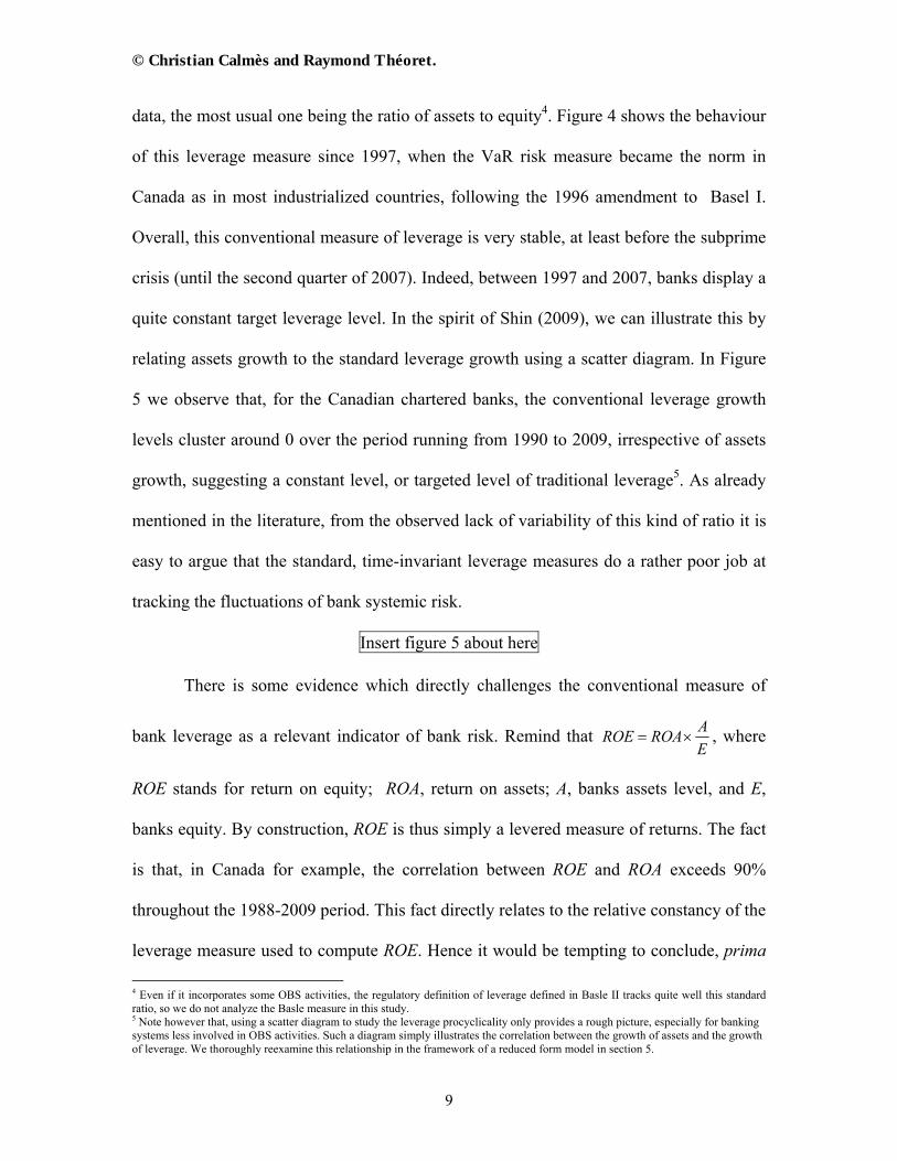
data, the most usual one being the ratio of assets to equity4. Figure 4 shows the behaviour
of this leverage measure since 1997, when the VaR risk measure became the norm in
Canada as in most industrialized countries, following the 1996 amendment to Basel I.
Overall, this conventional measure of leverage is very stable, at least before the subprime
crisis (until the second quarter of 2007). Indeed, between 1997 and 2007, banks display a
quite constant target leverage level. In the spirit of Shin (2009), we can illustrate this by
relating assets growth to the standard leverage growth using a scatter diagram. In Figure
5 we observe that, for the Canadian chartered banks, the conventional leverage growth
levels cluster around 0 over the period running from 1990 to 2009, irrespective of assets
growth, suggesting a constant level, or targeted level of traditional leverage5. As already
mentioned in the literature, from the observed lack of variability of this kind of ratio it is
easy to argue that the standard, time-invariant leverage measures do a rather poor job at
tracking the fluctuations of bank systemic risk.
Insert figure 5 about here
There is some evidence which directly challenges the conventional measure of
bank leverage as a relevant indicator of bank risk. Remind that A
ROE ROAE
, where
ROE stands for return on equity; ROA, return on assets; A, banks assets level, and E,
banks equity. By construction, ROE is thus simply a levered measure of returns. The fact
is that, in Canada for example, the correlation between ROE and ROA exceeds 90%
throughout the 1988-2009 period. This fact directly relates to the relative constancy of the
leverage measure used to compute ROE. Hence it would be tempting to conclude, prima
4 Even if it incorporates some OBS activities, the regulatory definition of leverage defined in Basle II tracks quite well this standard ratio, so we do not analyze the Basle measure in this study. 5 Note however that, using a scatter diagram to study the leverage procyclicality only provides a rough picture, especially for banking systems less involved in OBS activities. Such a diagram simply illustrates the correlation between the growth of assets and the growth of leverage. We thoroughly reexamine this relationship in the framework of a reduced form model in section 5.
© Christian Calmès and Raymond Théoret.
10
facie, that banks did not shift to riskier assets when their leverage constraint was
increasingly binding, and did not manage their standard leverage to boost their return on
equity before the 2007 credit crisis. However, in the United States, there is evidence that
financial intermediaries used their balance sheet leverage to increase their return on
equity (e.g. Stiroh 2004). We know that banks systemic risk was also trending upward in
Canada and elsewhere (Calmès and Liu 2009, Calmès and Théoret 2010) so returns had
to be somehow “levered”. With the help of OBS activities, banks might have levered the
return on their assets and boosted their stock returns. Unfortunately, the banks balance
sheet equity variable used in the standard leverage computation is actually inappropriate
to scale dollar earnings and properly detect these levered returns. The conventional
leverage ratio has to be modified to obtain a more appropriate measure of systemic risk.
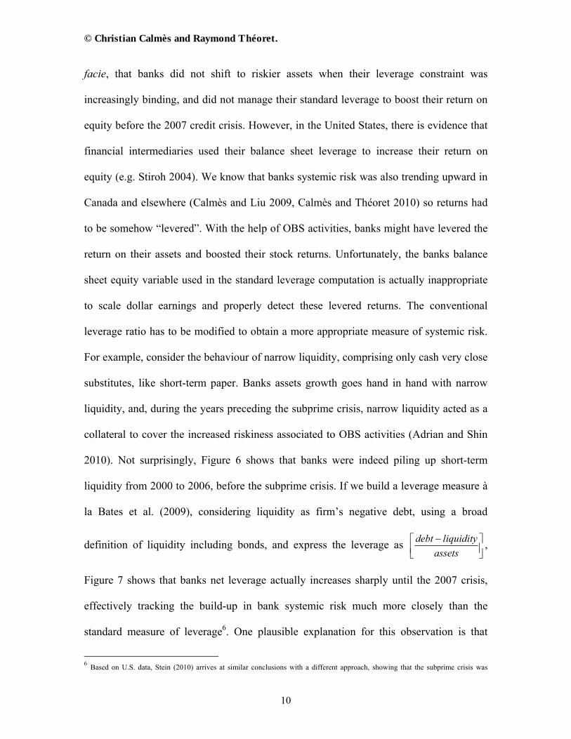
For example, consider the behaviour of narrow liquidity, comprising only cash very close
substitutes, like short-term paper. Banks assets growth goes hand in hand with narrow
liquidity, and, during the years preceding the subprime crisis, narrow liquidity acted as a
collateral to cover the increased riskiness associated to OBS activities (Adrian and Shin
2010). Not surprisingly, Figure 6 shows that banks were indeed piling up short-term
liquidity from 2000 to 2006, before the subprime crisis. If we build a leverage measure à
la Bates et al. (2009), considering liquidity as firm’s negative debt, using a broad
definition of liquidity including bonds, and express the leverage as debt liquidity
assets
,
Figure 7 shows that banks net leverage actually increases sharply until the 2007 crisis,
effectively tracking the build-up in bank systemic risk much more closely than the
standard measure of leverage6. One plausible explanation for this observation is that
6 Based on U.S. data, Stein (2010) arrives at similar conclusions with a different approach, showing that the subprime crisis was
© Christian Calmès and Raymond Théoret.
11
banks use a portion of their balance sheet liquidities to fund their OBS activities. As the
observed leverage constraint becomes more binding, and leverage converges
progressively towards the regulatory limit, liquidity can provide a capital regulatory
arbitrage by building a bridge between balance sheet and off-balance-sheet (Jones 2000,
Calomiris and Mason 2004, Ambrose et al. 2005, Kling 2009, Brunermeier 2010,
Cardone et al. 2010). In a sense, liquidity vanishes from the balance sheet and feeds into
OBS activities, and, consequently, the effective leverage automatically increases, even if
this does not show up in the standard accounting measures of bank leverage.
Insert figure 6 about here
In summary, the first reason why conventional measures of bank leverage based
on balance sheet ratios, such as the assets to equity ratio seem to be poor measures of
bank risk, is that banks tend to have a target leverage for this kind of measures, and,
consequently, the observed leverage does not detect whatever bank risk management
might be at play underneath.
3. Leverage elasticity measures, detrending and the Kalman Filter
A second reason why standard leverage measures may be found inappropriate to
assess bank risk is that these measures are essentially time-invariant. Compared to
accounting ratios, an elasticity measure of bank leverage seems a priori more suited to
measure the sensitivity of a key measure of bank performance Y – like earnings, net value
(net worth) or equity – to a “support” X, like assets or net operating income, because,
unlike the ratios based on balance sheet data, the computation of leverage elasticity
measures is free from questionable assumptions. For example, it is no longer necessary to
predictable on the basis of the leverage measure he develops, financial sector systemic risk being proportional to the excess leverage, measured as the difference between the observed leverage and the optimal one the author introduces.
© Christian Calmès and Raymond Théoret.
12
assume that the variation in equity captures all the changes in asset values, as is the case
with the asset to equity ratio. Elasticity leverage measures are also free of assumptions
regarding the relationship between Y and X (except, maybe, for the implicit assumption of
linearity), and as such, are better suited to evaluate the sensitivity of Y to X compared to a
simple Y/X ratio. In other words, elasticity measures of leverage tend to offer the
advantage of being time-varying and freely measuring the fluctuations of the Y to X
relation.
Insert figure 7 about here
3.1. Bank leverage elasticity measures
Leverage originates from the idea of lever in physics, which is the achievement of
a final outcome more than proportional to the force employed (DeMedeiros et al. 2009).
Any lever takes a support to magnify the initial force. In accounting and finance, the
support is generally given either by fixed assets or fixed costs (for operating leverage),
and by fixed payments and interest (for financial leverage). Relatedly, in economics and
finance, measures of leverage are based on elasticities. If the variable X has a leveraging
effect on the variable Y, we measure the resulting outcome by the elasticity of Y with
respect to X, defined as dY X
dX Y. However, in accounting and auditing, a simplifying
assumption is often considered, namely that dY dX . There is a straightforward
justification for this simplification: analysts are often more concerned by the time-
invariant, long-run value of leverage, and thus by the information conveyed by the
© Christian Calmès and Raymond Théoret.
13
average, constant risk value. Therefore, the computed leverage is simply equal to X
Y in
this case, with X and Y two stock or balance sheet variables. For example, as noted
earlier, in the banking industry, a conventional measure of leverage is the ratio of assets
to equity. In this case, the theoretical measure of leverage is the elasticity of equity with
respect to assets, that is, dE A
dA E, but, to simplify this leverage measure, practitioners
usually assume that dE dA (Breuer 2002). In other words, they implicitly assume that,
in the long-run, changes in assets are equal, or proportional, to changes in equity, so that
computing the elasticity of equity to assets boils down to the computation of the
conventional assets to equity ratio. Since, by accounting definition, assets are the sum of
debt and equity, this leverage measure is also equal to 1debt
equity , or to simplify further,
proportional to debt
equity. According to this accounting approach, the value of equity
captures all gains and losses on asset positions. Equity is thus considered, de facto, as a
residual (Breuer 2002). However, in practice, capital losses may well be funded by
additional debt or by assets sales without influencing equity, at least in the short-term.
And we may also imagine a lot of cases in which the relationship between the changes in
assets and the changes in equity is really not a one-for-one mapping. In this respect, to
really cast leverage in a financial stability framework and better capture the fluctuations
of banking risk, it is necessary to modify the standard balance sheet leverage ratios and
rely on elasticity measures of leverage. As a benchmark, we compute the banks elasticity
of equity to assets to study the extent to which the drawbacks of the regular assets to
equity ratio can be avoided with its associated time-varying, elasticity counterpart. We
© Christian Calmès and Raymond Théoret.
14
also analyze two other traditional leverage measures: i) the elasticity of net value to
assets, net value being an economic measure of equity value or wealth; and ii) the degree
of total leverage, DTL, introduced by DeYoung and Roland (2001), defined as the
elasticity of net earnings to operating income. We then consider two elasticity measures
related to OBS activities, namely the elasticity of net earnings to noninterest income, and
the elasticity of noninterest income to net interest income. In essence, we follow the
Griffin and Dugan (2003) approach throughout, and study degrees of economic leverage
(DEL), i.e. indicators describing the average sensitivity of one variable to a change in
another, after removing the trend of the two variables.
3.2 Leverage detrending
Since the time series used to compute leverage measures are often non-stationary,
it is desirable to detrend them, a matter first addressed by Mandelker and Rhee (1984),
and O'Brien and Vanderheiden (1987). Otherwise, in the leverage computation, the trend
in the elasticity measure of leverage, as generally captured by the ratio of the variables
levels X/Y, would completely dominate the cyclical part. This is precisely why, for
convenience, financial analysts and practitioners can rightfully omit the ratio of variables
differentials appearing in the elasticity formulation of leverage, dY/dX, and approximate
by a simple X/Y ratio. But our case is different. We are interested by measures of bank
risk which can help detect bank true risk, and we also want to comprehensively study the
relative performance of measures able to capture the cyclical behaviour of leverage and
the information conveyed by the short-term changes in leverage, especially at business
© Christian Calmès and Raymond Théoret.
15
cycle frequencies. Consequently, we have to address the question of detrending carefully.
First remark that an elasticity computed on raw time series tends to measure the
differences in trends between the series. Obviously, if the trends are similar, the elasticity
measure will be close to 1 (Mandelker and Rhee 1984). This is typically what happens
with standard accounting, time-invariant, long-term measures of leverage. In general, this
level of 1 is the computed benchmark reached when risk converges to zero. For instance,
theoretically, the degree of a firm’s operating leverage is equal to unity if fixed costs (or
fixed assets) are zero. There is no operating risk in this case. However, when the time
series are detrended, if, on the one hand, the elasticity becomes a more suitable measure
of the marginal sensitivity of the variable relative to its support, as expressed by the
percentage deviations observed in these variables, on the other hand, in this case, the unit
benchmark level of leverage is no longer applicable.
Second, note that, in the literature on leverage, the authors often ignore that the
detrending method used to extract the cyclical components of the leverage time series
may influence the results (Cooley 1996, Canova 1998). In fact, it is much preferable to
rely on several detrending methods to help control for the influence of detrending on the
leverage dynamics. We begin with a leverage detrending method first introduced by
Mandelker and Rhee (1984), and O'Brien and Vanderheiden (1987), a method referred to
the logarithmic residuals detrending method. To compute the elasticity of the variable Y
with respect to the variable X, the authors detrend the series with the following set of
regressions:
0 1log( ) , 1,2,...,t tY trend t N (1)
0 1log( ) , 1,2,...,t tX trend t N (2)
© Christian Calmès and Raymond Théoret.
16
where trend is a trend variable scaled from 1 to N. Then, the authors run an ordinary least
squares (OLS) regression on the residuals to obtain the elasticity coefficient:
0log logt t t (3)
In some sense, the estimated ̂ , the elasticity of Y to X, is a “marginal elasticity”
capturing the variations in the X-Y relationship.
Another standard procedure found in the literature resorts to polynomials
detrending, for instance the cubic detrending method. As with the logarithmic residuals,
the method is based on the following equations:
2 30 1 2 3log( ) , 1,2,...,t tY trend trend trend t N (4)
2 30 1 2 3log( ) , 1,2,...,t tX trend trend trend t N (5)
As in the previous case, the elasticity coefficient is then obtained by running an
OLS regression on the residuals using equation (3). DeYoung and Roland (2001) provide
a good example of the application of this technique to the study of banks total leverage,
although the authors rely on a modified version of the cubic detrending to accommodate
the negative numbers associated to banks losses. More precisely, in their regressions, the
variables are expressed in levels instead of logarithms7. The elasticity measure they
derive from the residuals is defined as: ˆ Xelasticity
Y , where ̂ is the estimated
coefficient obtained from the residuals regression, and X and Y are respectively the
mean values of X and Y computed over the sample period. In our study, we consider both
cubic detrending methods to document the relative performance of the various leverage
measures we analyze. To distinguish the DeYoung and Roland (2001) cubic detrending
7 Note also that the fact that their residuals are computed on variables expressed in levels instead of logarithms causes some problems when filtering, as the series ratio tend to fluctuate too much.
© Christian Calmès and Raymond Théoret.
17
method from the regular logarithmic cubic detrending method, we call the former the
cubic level detrending method and the latter the cubic logarithmic detrending method. In
addition to these three detrending methods, we also consider two other common
techniques. In the first approach, the series are directly detrended using first-differences,
as often applied to non-stationary time series. In this case, we compute the leverage as
Y Xelasticity
X Y
, where Y and X are respectively the first-differences of the
variables Y and X. The last method we use consists in detrending the logarithms of Y and
X using the Hodrick-Prescott filter8, then computing the elasticity coefficient with
equation (3).
3.3 Optimal bank leverage measurement
Many studies on bank leverage usually consider static indicators, accounting
indicators fairly constant over time. Nevertheless, the effective leverage is time-varying,
and a dynamic, not a static measure. Hence, to completely challenge the traditional
leverage ratios used to measure bank risk we also have to evaluate the relative
performance of dynamic leverage measures. To study the dynamics of bank leverage
measures, we apply a Kalman filter approach, as it is one of the best ways to model
regressors coefficient dynamics and time-varying parameters. We introduce two
equations to implement the filter (i) the signal equation, equation (6), and (ii) the state
variable equation, equation (7), where the state variable represents the leverage measure
8 With a smoothing parameter λ equal to 1600. As a robustness check, we also try other parameter values but the standard one seems to perform quite well.
© Christian Calmès and Raymond Théoret.
18
itself. Leverage is thus computed optimally from one period to the next. For example, in
the case of the simple logarithmic residuals detrending method, the signal equation reads:
0log logt t t tlev (6)
which is basically equivalent to the residuals equation, i.e., equation (3), and leverage,
levt, fluctuates from one period to the next following the state variable equation:
1t t tlev lev (7)
where t is the innovation term. Hence, as often assumed in the Kalman filter literature,
we model the state variable, leverage in our case, as a simple random walk.
There is an alternative way to compute time-varying coefficients which is not
systematically used in this paper9 but is worth mentioning: the conditional approach
(Ferson and Schadt 1996, Christopherson et al. 1998, Ferson and Qian 2004). The
Kalman filter method may be viewed as a smoothed version of this approach as, similarly
to the Kalman filter approach, in a conditional model the coefficients are updated each
period following the arrival of new information. To cast the leverage equation in a
conditional model, equation (3) can be rewritten:
0log logt t t t (8)
Leverage, which is equal to θt, is indexed by time to indicate that it is a time-varying
coefficient conditional on the information set available at time t. Assume that θt is related
to a vector of control variables Zt such that:
0t t tZ ω (9)
9 We actually checked the robustness of our results with this method. Since the message is basically the same, the associated results are not reported. However, we discuss the results obtained using this method for the degree of total leverage (DTL), one of our favourite measures, in the empirical section.
© Christian Calmès and Raymond Théoret.
19
where νt is the innovation. To estimate the coefficients vector ω , we can substitute
equation (9) in equation (8), and equation (10) obtains:
0 0log log logt t t t tZ ω (10)
Equation (10) is then estimated using the OLS method. The coefficients of equation (9),
the time-varying leverage, are perfectly identified.
4. Empirical results
4.1. Data
The data used in this study are composed of two samples, 1990-2009, and 1997-
2009. The first sample is drawn from the National balance sheet accounts produced by
CANSIM, a Statistics Canada database first published in 1990. We use the quarterly
sample until 2009 to compute the leverage measure defined as the elasticity of net value
to assets. However, the other aggregate measures of leverage require the Canadian banks
financial results, which are not available in the National balance sheet accounts.
Moreover, Statistics Canada provides no comprehensive database on banks financial
results. Bankscope offers statistics on Canadian banks financial results, but the series
cover only a short period of time. We thus directly hand-collect and build the relevant
data recorded over the years from the various associations and institutes providing data,
in particular the Canadian Bankers Association and the Office of the Superintendant of
financial institutions. Our quarterly series are provided for the eight major banks, which
account for more than 90% of the Canadian banks aggregate assets, by the Canadian
© Christian Calmès and Raymond Théoret.
20
Bankers Association, for the period running from the first quarter of 1997 to the first
quarter of 2009.
4.2. OLS estimation Table 1 provides the OLS estimation results for the five leverage measures we
study. First note that three estimated non-detrended leverage measures, displayed on the
bottom panel – the elasticity of net earnings to total operating income (ξearn-totinc), the
elasticity of net earnings to noninterest income (ξearn-noninc), and the elasticity of equity to
assets (ξeq-assets) – are close to 1, suggesting that the trends of the underlying series might
be similar. The non-detrended elasticity of net value to assets (ξNV-assets), estimated over a
longer period, is equal to 1.57, a greater level which suggests that the trends of net value
and assets could be different. Finally, the elasticity of noninterest income to interest
income (ξnoninc-inc) is positive but quite lower than 1, so that the trends of these two
variables should also be different.
Insert Table 1 about here
Second, when looking at the detrended leverage measures, note that the sign of the
measures is generally robust to the detrending method used, but that the estimated
leverage level is somewhat sensitive to the detrending method. Note also that, for three
measures, the elasticity of net value to assets (ξNV-asets), the elasticity of earnings to total
operating income (ξearn-totinc), and the elasticity of earnings to noninterest income
(ξearn-noninc), the detrended estimated elasticities are greater than one. Moreover, the
estimated “balance sheet” elasticity leverage measure generally associated to the standard
leverage, i.e. the elasticity of equity to assets (ξeq-assets), is much lower than one, while the
© Christian Calmès and Raymond Théoret.
21
detrended elasticity of noninterest income to interest income (ξnoninc-inc) is negative, a sign
opposite to its non-detrended counterpart.
In terms of detrending, Table 1 shows that the simple logarithmic residuals
detrending method sometimes delivers leverage levels much lower than the other
methods. In particular, it delivers a coefficient lower than 1 for the elasticity of earnings
to total income (ξearn-totinc), and for the elasticity of earnings to noninterest income
(ξearn-noninc), while the coefficients are greater than 1 with the other detrending methods.
For instance, using the simple logarithmic residuals method, the elasticity of net earnings
to total income (ξearn-totinc) is 0.98, while it is around 2 with the four other detrending
methods. Since this detrending method is based on the residuals of the regression of the
series logarithms, it might not properly capture the growth rates nonlinearity of the series
compared to more sophisticated detrending methods, such as the Hodrick-Prescott (HP)
filter and the cubic detrending method.
Turning to the relative performance of the elasticity leverage measures, when
looking at the elasticity of net value to assets (ξNV-assets), while it presents the highest
average estimates, it is also the leverage measure the most sensitive to the detrending
method. Over the period 1997-2009, its lowest value, at 2.62, is associated to the first-
differences detrending method, while its highest, 5.79, is delivered by the cubic level
detrending method. This illustrates the extent to which the detrending method can
influence the estimation results. By contrast, one of the most popular leverage measures,
the degree of total leverage, i.e. the elasticity of earnings to total operating income
(ξearn-totinc), displays quite consistent results regardless of the detrending approach. For
four detrending methods, despite the low R2, the estimated leverage, systematically
© Christian Calmès and Raymond Théoret.
22
significant at the 95% confidence level, is approximately equal to 2. This result indicates
that the degree of total leverage is generally high, which suggests a quite high level of
bank risk over the 1997-2009 sample period. Finally note that the elasticity of equity to
assets (ξeq-assets) seems less robust than the other reported measures. Without detrending,
this elasticity measure, which is then basically the conventional measure of bank risk, is
close to 1, suggesting that the trends of assets and equity are quite similar. Once
detrended however, this elasticity is equal to 0.18 using the HP filter, being significant at
the 95% confidence level, and to 0.58, significant at the 90% confidence level with the
simple logarithmic residuals detrending method. Moreover, the elasticity coefficient is no
longer significant when using the two other detrending methods. In other words, contrary
to the other elasticity measures, the elasticity version of the most commonly used
leverage measure, the ratio of assets to equity, is much lower than one. This low elasticity
value might relate to uncaptured nonlinearities in banks balance sheet data. More
importantly, considering that bank systemic risk has been increasing throughout the
sample period, pari passu, with the growth in OBS activities, this low leverage level
supports the idea that the equity-assets ratio is not suited to properly assess the stance of
the banking system stability.
In summary, our OLS estimations confirm the influence of the detrending method
on the estimation of the leverage measures. In particular, it is preferable to rely on
methods which best capture the nonlinearities associated to the growth of the series
considered. On the basis of our experiments, the simple logarithmic residuals detrending
method does not seem to be particularly satisfactory on this dimension, having a tendency
to systematically underestimate the leverage measures. By contrast, the HP filter, and the
© Christian Calmès and Raymond Théoret.
23
cubic level and cubic log detrending methods do a better job10. Regarding the different
leverage measures we study, we find that the degree of total leverage is rather high during
the sample period. This result is quite consistent with the fact that the weight of OBS
activities is increasing throughout the period, leading to an increased riskiness in the
banking industry. However, with OLS, we only estimate punctual measures of bank
leverage. The implicit averaging process embedded in these estimations may hamper the
performance of some detrending methods, or partly mask the true performance of our
measures compared to what a dynamic setting might reveal. This aspect is analyzed in the
following section.
4.3. Time-varying leverage and the Kalman Filter
As argued by DeYoung and Roland (2001), an implicit assumption underlying the
OLS estimations of bank leverage measures is that banks have a stable product-mix, and
stable parameters values describing their behaviour. However, because of the growing
volatility of banks financial data, and the changing banking landscape, this assumption
ought to be relaxed (Calmès and Théoret 2010, Nijskens and Wagner 2010). In fact, far
from being stable, bank leverage measures are quite changing and procyclical (Shin
2009). To investigate this question, we “dynamize” our bank leverage measures with the
help of equations (6) and (7), and Kalman filtering. Given their superior performance,
two leverage measures are studied in detail with the five detrending methods reported in
Table 1: the elasticity of net value to assets, and the degree of total leverage (DTL). We
also report the Kalman filter measures for the other leverage measures, but only with the
10 Incidentally, the two cubic detrending methods deliver very similar results for the various leverage measures using OLS estimation.
© Christian Calmès and Raymond Théoret.
24
Holdrick-Prescott filter (HP), one of our preferred detrending methods given its overall
performance in OLS estimations, and its ability to track time series fluctuations.
Insert Figure 8 about here
To be consistent with the recent banking history, we expect our Kalman-filtered,
detrended elasticity measures to be on an upward trend after the Asian crisis of 1997 and
until 2007, just before the subprime crisis, since bank systemic risk was obviously
moving on an upward trend during this period, both in the U.S. (Rajan 2005, Adrian and
Shin 2010, Blanchard 2009, Rajan 2009, Nijskens and Wagner 2010), in Canada (Calmès
and Théoret 2010) and elsewhere. Figure 8 reports the Kalman-filtered bank leverage
measured with the non-detrended and detrended elasticity of net value to assets (ξNV-assets),
the most “elastic” measure according to our OLS regressions. The non-detrended
measure is taken as a benchmark. This measure shows no particular cycle although it
collapses during the two crises of the sample period, namely the 1997 Asian crisis and the
2007 subprime crisis. These lows, associated to deleveraging episodes, are also shared by
the detrended leverage measures, except for the first-differences detrending method,
which, incidentally, systematically delivers bad results for all the elasticities measures, as
it tends to overstate fluctuations at high frequencies. In Figure 8, we can observe that the
simple logarithmic detrending method tends to display a very smooth pattern for the ξNV-
assets leverage measure. After 2002, a year of slow economic activity, the evolution of this
detrended leverage measure is quite in line with the increase in bank systemic risk,
showing an upward leverage trend until the subprime crisis, and a substantial drop after.
More importantly, note that similar patterns obtain with the HP detrending and the cubic-
log detrending methods, which both provide the most consistent indicators. In this
respect, the leverage appears quite stable until the Asian crisis when it falls sharply.
© Christian Calmès and Raymond Théoret.
25
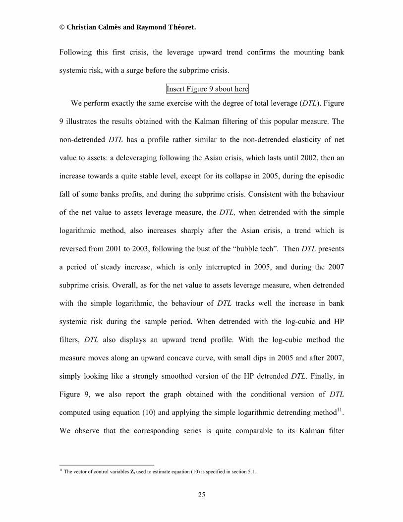
Following this first crisis, the leverage upward trend confirms the mounting bank
systemic risk, with a surge before the subprime crisis.
Insert Figure 9 about here
We perform exactly the same exercise with the degree of total leverage (DTL). Figure
9 illustrates the results obtained with the Kalman filtering of this popular measure. The
non-detrended DTL has a profile rather similar to the non-detrended elasticity of net
value to assets: a deleveraging following the Asian crisis, which lasts until 2002, then an
increase towards a quite stable level, except for its collapse in 2005, during the episodic
fall of some banks profits, and during the subprime crisis. Consistent with the behaviour
of the net value to assets leverage measure, the DTL, when detrended with the simple
logarithmic method, also increases sharply after the Asian crisis, a trend which is
reversed from 2001 to 2003, following the bust of the “bubble tech”. Then DTL presents
a period of steady increase, which is only interrupted in 2005, and during the 2007
subprime crisis. Overall, as for the net value to assets leverage measure, when detrended
with the simple logarithmic, the behaviour of DTL tracks well the increase in bank
systemic risk during the sample period. When detrended with the log-cubic and HP
filters, DTL also displays an upward trend profile. With the log-cubic method the
measure moves along an upward concave curve, with small dips in 2005 and after 2007,
simply looking like a strongly smoothed version of the HP detrended DTL. Finally, in
Figure 9, we also report the graph obtained with the conditional version of DTL
computed using equation (10) and applying the simple logarithmic detrending method11.
We observe that the corresponding series is quite comparable to its Kalman filter
11 The vector of control variables Zt used to estimate equation (10) is specified in section 5.1.
© Christian Calmès and Raymond Théoret.
26
countepart, except that it is more volatile and that the deleveraging period associated to
the subprime crisis seems more pronounced according to the conditional DTL.
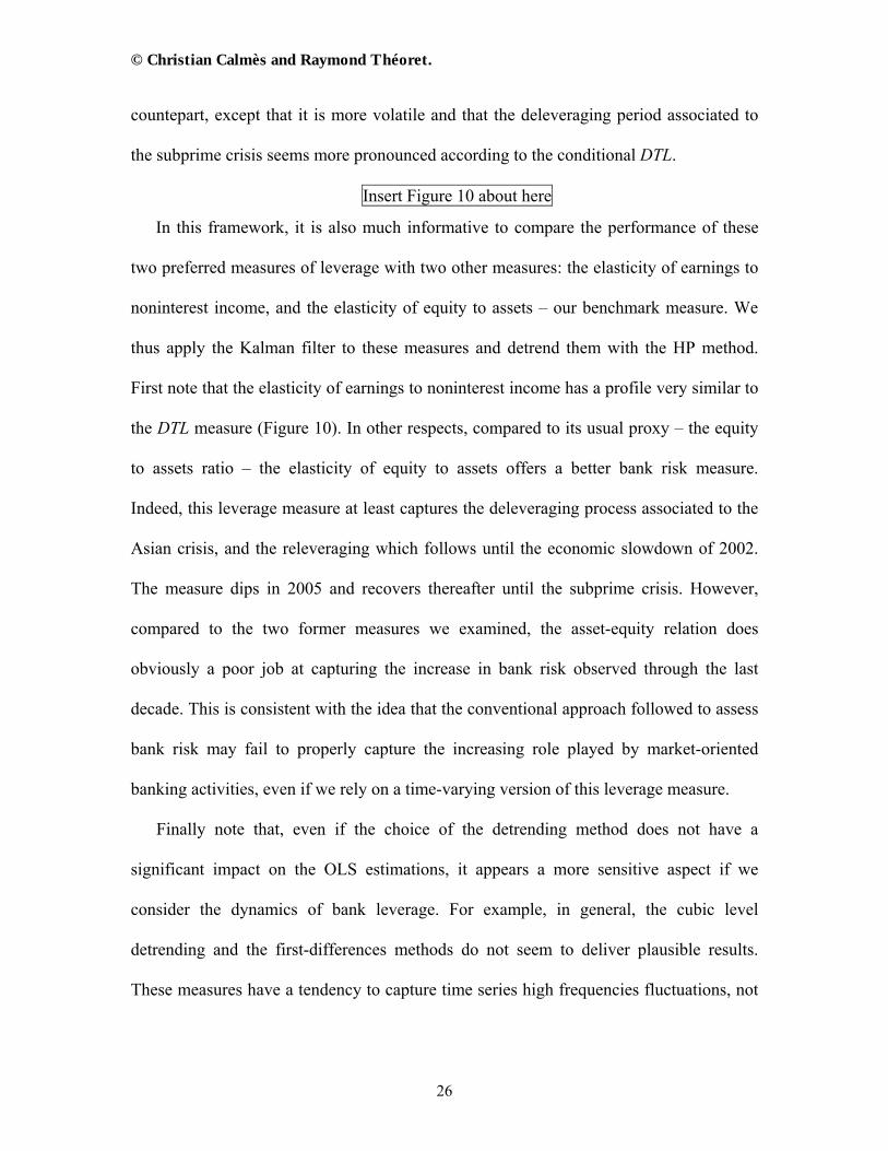
Insert Figure 10 about here
In this framework, it is also much informative to compare the performance of these
two preferred measures of leverage with two other measures: the elasticity of earnings to
noninterest income, and the elasticity of equity to assets – our benchmark measure. We
thus apply the Kalman filter to these measures and detrend them with the HP method.
First note that the elasticity of earnings to noninterest income has a profile very similar to
the DTL measure (Figure 10). In other respects, compared to its usual proxy – the equity
to assets ratio – the elasticity of equity to assets offers a better bank risk measure.
Indeed, this leverage measure at least captures the deleveraging process associated to the
Asian crisis, and the releveraging which follows until the economic slowdown of 2002.
The measure dips in 2005 and recovers thereafter until the subprime crisis. However,
compared to the two former measures we examined, the asset-equity relation does
obviously a poor job at capturing the increase in bank risk observed through the last
decade. This is consistent with the idea that the conventional approach followed to assess
bank risk may fail to properly capture the increasing role played by market-oriented
banking activities, even if we rely on a time-varying version of this leverage measure.
Finally note that, even if the choice of the detrending method does not have a
significant impact on the OLS estimations, it appears a more sensitive aspect if we
consider the dynamics of bank leverage. For example, in general, the cubic level
detrending and the first-differences methods do not seem to deliver plausible results.
These measures have a tendency to capture time series high frequencies fluctuations, not

© Christian Calmès and Raymond Théoret.
27
business cycles fluctuations12. The Kalman filter, used in conjunction with the other
detrending methods performs very well, and happens to be a very powerful tool to
analyse the cyclical patterns of bank leverage. Relying on this framework, we can argue
that, in addition to being procyclical, as evidenced in the literature (e.g. Adrian and Shin
2010), our bank leverage measures appear to be forward-looking indicators well tracking
systemic risk.
5. The cyclical pattern of bank leverage
In this section, we cast bank leverage in a reduced form model to document the
cyclical role played by the share of noninterest income (i.e., the income OBS activities
generate) and liquidity variables. We first apply this model to the banks observed
leverage, that is, the ratio of assets to equity, and then test the same model on the
simulated series of the banks degree of total leverage, DTL (the elasticity of earnings to
net operating income), applying the Kalman filter to two detrended measures of DTL, the
residuals logarithmic and the HP detrending methods. We also apply this reduced form
model to two filtered leverage measures based on balance sheet data, the elasticity of net
value to assets, and the benchmark elasticity measure, the elasticity of equity to assets.
5.1 Estimation of the standard leverage measure
12 According to Cooley and Prescott: “The first-differences filter leads to more short-term fluctuations than does the H-P filter. This is to be expected since the latter filter emphasizes the high-frequency movements more. Correspondingly, it can be seen that the H-P filtered data display more serial correlation.” (Cooley, 1995, 28-29).
© Christian Calmès and Raymond Théoret.
28
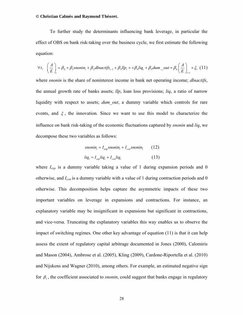
To further study the determinants influencing bank leverage, in particular the
effect of OBS on bank risk-taking over the business cycle, we first estimate the following
equation:
0 1 2 1 3 4 5 61
, _t t t t tt t
A At snonin dlnactifs llp liq dum out
E E
(11)
where snonin is the share of noninterest income in bank net operating income; dlnactifs,
the annual growth rate of banks assets; llp, loan loss provisions; liq, a ratio of narrow
liquidity with respect to assets; dum_out, a dummy variable which controls for rare
events, and , the innovation. Since we want to use this model to characterize the
influence on bank risk-taking of the economic fluctuations captured by snonin and liq, we
decompose these two variables as follows:
expt t con tsnonin I snonin I snonin (12)
t exp t con tliq I liq I liq (13)
where Iexp is a dummy variable taking a value of 1 during expansion periods and 0
otherwise, and Icon is a dummy variable with a value of 1 during contraction periods and 0
otherwise. This decomposition helps capture the asymmetric impacts of these two
important variables on leverage in expansions and contractions. For instance, an
explanatory variable may be insignificant in expansions but significant in contractions,
and vice-versa. Truncating the explanatory variables this way enables us to observe the
impact of switching regimes. One other key advantage of equation (11) is that it can help
assess the extent of regulatory capital arbitrage documented in Jones (2000), Calomiris
and Mason (2004), Ambrose et al. (2005), Kling (2009), Cardone-Riportella et al. (2010)
and Nijskens and Wagner (2010), among others. For example, an estimated negative sign
for 1 , the coefficient associated to snonin, could suggest that banks engage in regulatory

© Christian Calmès and Raymond Théoret.
29
capital arbitrage, increasing their involvement in OBS activities to artificially decrease
their observed leverage and bypass their capital requirement constraint. Another variable
we consider to analyze leverage cyclical pattern is the growth of banks assets, dlnactifs.
According to Adrian and Shin (2010), an increase in assets growth should increase
leverage and contributes to the leverage procyclicality. The third variable which can
influence bank risk-taking over the business cycle is loan loss provisions, llp. When
banks face increased risk, they have an incentive to lower their leverage to counter the
mounting level of llp. Consequently, we can expect a negative sign for β3. Finally, as
discussed earlier, liquidity is likely to be an important factor impacting leverage,
especially in the context of shadow banking. For example, we can anticipate that liquidity
and leverage comove negatively during contraction periods, when banks deleverage and
simultaneously boost their liquidity to avoid insolvency.
Insert table 2 about here
Table 2 provides the OLS estimation of equation (11) over the period 1997-2009.
The performance of the estimation is quite good according to the adjusted R2, at 0.80, and
the explanatory variables are mostly significant at the 99% confidence level. The
residuals heteroskedasticity is treated with the White consistent covariance matrix. There
is no evidence of residuals autocorrelation, the DW statistic being equal to 1.76. In Table
2, first note that, as expected, the asset growth variable (dlnactifs) positively contributes
to leverage. Its coefficient is significantly positive and equal to 0.18. We also find that the
llp variable decreases leverage, its coefficient being equal to -2.48, and significant at the
99% confidence level. More importantly, the estimated coefficient of snonin is
significantly negative at the 99% confidence level, and for example equal to -8.81 in
expansions, which supports the idea that banks might indeed rely on OBS activities to
© Christian Calmès and Raymond Théoret.
30
engage in regulatory capital arbitrage (Nijskens and Wagner 2010). In contractions, the
estimated snonin coefficient, at -8.70, is not very different from its expansion level, so
that the arbitrage always exerts a downward pressure on the asset to equity ratio. What
might likely happen is that, during contractions, on-balance-sheet assets rebalance,
ceteris paribus, as securitization decreases and assets are repatriated from off-balance-
sheet. The similarity of the coefficient (in expansions versus contractions) also suggests
that the standard leverage measure does not capture any particular asymmetric impact of
snonin, a finding consistent with the fact that the general fit of the model is almost the
same if the regime shifts are not accounted for. Finally note that the coefficient associated
to the narrow measure of short-term liquidity (comprising cash and short-term paper), at
-29.92, is only significant in contraction periods (Table 2). In these periods, banks can
hardly rely on their assets as collateral to extend their borrowings because of the
important losses on assets they face. Hence, they have to increase their liquidity, while at
the same time decreasing their leverage to strengthen their balance sheet and regain
profitability. In this respect, an increase in liquidity, like the injections performed by
central banks during the subprime crisis, might facilitate the deleveraging process by
fostering orderly sales of assets, as the spread between assets market value and their
fundamental value could then be reduced. In any case, more liquidity goes hand-in-hand
with deleveraging during bad times (Uhlig 2010).
© Christian Calmès and Raymond Théoret.
31
5.2 Estimation of the degree of total leverage measures
Table 3 reports our results for the DTL leverage measure when we apply equation
(11) to the measures obtained respectively with the logarithmic residuals, i.e. simple
logarithmic, and the HP detrending methods.
Insert Table 3 about here
A first glance at the estimations shows that the equations perform better when
distinguishing expansions from contractions, which was not the case for the standard
measure of leverage. For instance, in the case of the simple logarithmic DTL, the R2
increases from 0.55 to 0.72 when accounting for cyclical phases, and the DW statistic
increases from 1.64 to 1.75, which also suggests a better specification of the model
including the cyclical regimes. In the case of the HP DTL, the R2 raises from 0.62 to 0.76
when using cyclical regime shifts, while the DW increases from 1.60 to 1.85. More
importantly, with the DTL filtered measure obtained by the simple logarithmic detrending
method, Table 3 indicates that DTL sensitivity to snonin is positive in expansions and
contractions, the estimated coefficients being respectively 1.98 and 0.99, and significant
at the 99% confidence level. In other words, this result suggests that a greater reliance on
OBS activities increases the effective leverage, and particularly so in expansions. This
positive relationship contrasts with the negative coefficients obtained with the standard
measures of leverage (time-varying or not), as it unveils directly the influence of OBS
activities on bank risk. To understand the intuition better, we can proxy the DTL
measures by the y
x ratio of earnings to revenue. Given the direct link between this
leverage measure and the ratio r
( for earnings, r for revenues), estimating this ratio
© Christian Calmès and Raymond Théoret.
32
can shed more light on the determinants of the DTL measure. The estimation results of
this ratio using the same specification (equation (11)) are reported in Table 4. Note that
similarly to what obtains with the regular DTL measures, the impact of snonin on r
is
positive, and greater in expansions than in contractions. An increase in snonin leads to an
increase in r, but, at the same time, it also increases the r
ratio because the activities
related to snonin are riskier than the traditional banking business lines, consequently
requiring a higher risk premium (Calmès and Théoret 2010). Furthermore, the fact that
r
is less sensitive to snonin in contractions than in expansions suggests that banks can
partly shield their profits in downturns, for instance by relying on derivatives, or by
arbitraging between financial and operating leverage (Mandelker and Rhee 1984). This
observation is also due to the fact that snonin is much lower in contractions than in
expansions, which imparts an asymmetric profile to DTL.
Insert Table 4 about here
Turning to the influence of liquidity on leverage, our results suggest that liquidity
also displays an asymmetric effect on DTL (Table 3). An increase in the ratio of liquidity
reduces DTL in expansions, while it increases it in contractions, the coefficients being
respectively -18.23 and 1.82, although the latter is not significant. To explain this
asymmetric behaviour, we can once again rely on the analysis of the r
ratio (Table 4).
Liquidity seems to have a higher opportunity cost during expansions, and tends to
effectively decrease DTL, ceteris paribus, while in contractions, the liquidity constraint is
more likely binding so that an increase in liquidity could help slacken the financing
© Christian Calmès and Raymond Théoret.
33
constraint, increasing the r
ratio and DTL. In summary, increases in the liquidity ratio
decreases DTL in expansions and increases it in contractions, a property opposite to, and
partly mitigating the impact of snonin on bank risk.
Finally, note that our findings do not seem to be much influenced by the
detrending method in general. For example, as in the case of the simple logarithmic
detrending method, liquidity also impacts negatively the HP detrended measure of total
leverage in expansions, its coefficient being equal to -23.99 and significant at the 99%
confidence level. The corresponding coefficient in contractions is also not significant
(Table 3). The snonin has a positive impact on the HP filtered detrended DTL during
expansions, the coefficient being 0.85 and significant at the 99% confidence level,
although the corresponding coefficient is negative but not significant in contractions, a
discrepancy which could be attributed to the more capricious nature of the HP filter
compared to the smooth simple-log.
5.3 Net value to assets and equity to assets elasticities We apply equation (11) to two other measures of leverage based on balance sheet
data, the elasticity of net value to assets and the elasticity of equity to assets. These
measures are the Kalman filtered, HP detrended series (Figures 8 and 9).
Insert Table 5 about here
As Table 5 indicates, and contrary to what we observe with the DTL measures and
the elasticity of equity to assets, the snonin coefficient is greater in contractions than in
expansions for the elasticity of net value to assets – the coefficients, significant at the
99% confidence level, being respectively 18.90 and 10.60. Qualitatively however, this
© Christian Calmès and Raymond Théoret.
34
variable has the same positive impact on leverage, both in expansions and contractions.
Similarly to what we observe with the DTL measures, liquidity has also an overall
negative impact on the leverage measure based on the elasticity of net value to assets, the
estimated coefficient for this variable being equal to -34.19 and significant at the 99%
confidence level13. However, the cyclical effect of liquidity on this leverage measure
seems to quantitatively differ from the one it has on DTL and on the elasticity of equity to
assets, for which the negative impact of liquidity is larger in expansion periods. Indeed,
for the elasticity of net value to assets, the coefficient of the liquidity ratio is greater in
absolute value in contractions than in expansions, the coefficients being respectively
-71.60 and -61.87. This might well coincide with the influence of snonin on the elasticity
of net value to assets, which is also more pronounced in contractions than in expansions.
One plausible explanation of this joint behaviour is that the elasticity of net value to
assets tends to be more sensitive to the deleveraging process occurring during downturns.
As evidence of this, during the 2007-2009 subprime crisis, the ratio of net value to assets
dropped sharply from a high of 4.2% in the second quarter of 2007 to a low of 1% in the
first quarter of 2009, and this development was accompanied by a sharp increase in
liquidity. These results could thus to be expected, as a decrease in the ratio of net value to
assets is systematically associated to a decrease in the elasticity of net value to assets.
Regarding the elasticity of equity to assets, first note that the behaviour of this
leverage measure is close to the one described for the DTL measures. In particular, the
overall sensitivity of this elasticity to snonin is positive, equal to 0.24, and significant at
the 99% confidence level, which, again, suggests that, ceteris paribus, OBS activities
13 Note that in the case of the elasticity of net value to assets, we resort to a broad measure of liquidity because a narrow measure yields insignificant coefficients.

© Christian Calmès and Raymond Théoret.
35
tend to increase bank risk. In this respect note that, compared to the standard equity to
assets ratio, the positive sign of β1 suggests that the elasticity version of the standard
leverage is more consistent with the influence of OBS activities on leverage, despite its
previously documented lack of variability and robustness. Also in line with the results
obtained for the DTL measures, we find that the coefficient of snonin is greater in
expansions than in contractions, the coefficients, both significant at the 99% confidence
level, being respectively 0.51 and 0.16. Relatedly, and again similarly to what obtains
with the DTL measures, liquidity impacts negatively on bank leverage in expansions, and
positively in contractions, suggesting that the risk-return trade-off and the opportunity
cost are more at play in expansions, whereas in contractions the binding liquidity
constraints seem to play a primary role.
In summary, the noninterest income generated by banks OBS activities has a
tendency to influence the cyclicality of all the leverage elasticity measures we analyze. In
particular, our experiments results suggest that the impact of snonin on leverage is
generally higher in expansions than in contractions. Previous studies have already
established that the growing share of noninterest income increases the volatility of bank
operating revenues (Stiroh and Rumble 2006, Calmès and Théoret 2010), and we find
that this development might actually have a cyclical pattern too (Heaton et al. 2010). This
dynamics is important to document further because leverage contributes substantially to
the pricing and the volatility of financial assets, and to the formation of the risk premia
(Danthine and Donaldson 2002, Geanakoplos 2010) which increase the funding costs of
financial institutions.
© Christian Calmès and Raymond Théoret.
36
6. Conclusion
In spite of the important impact of OBS activities on bank risk, papers focusing on
banks OBS-induced leverage are quite rare. To the best of our knowledge, our article
provides the first comprehensive study of bank aggregate leverage measures in a dynamic
setting designed, in part, to thoroughly analyze the time-varying influence of market-
oriented activities on leverage. In particular, we show that the conventional measures
regulated by the Basle Agreements are not necessarily good measures of bank risk. Our
results suggest that the main drawback of these measures might be that they are
manipulated at target levels to comply with regulatory constraints, so that, by
construction, they cannot really detect regulatory capital arbitrage. Since this arbitrage
and the high risk to which it is associated are much enhanced by OBS practices, it is
important to account for the role played by noninterest income more directly in order to
get a reliable picture of bank true leverage.
The findings we report in this study also indicate that the cyclical behaviour of
bank leverage seems conditioned by the detrending method, especially when using
Kalman filtering. In this respect, the HP filter and the simple logarithmic-residuals
detrending method seem to outperform the other methods we consider. Regarding the
overall quality and performance of the various leverage measures we analyze throughout
this study, we would favour the degree of total leverage and the elasticity of net value to
assets as the best measures of bank systemic risk. When estimated over the whole sample
period, these elasticities, which incidentally record high levels of leverage regardless of
the detrending method used, were clearly moving on a steep upward trend before the
© Christian Calmès and Raymond Théoret.
37
subprime crisis, a phenomenon hardly captured by the conventional leverage measure. In
other respects, when we proxy the ratio of assets to equity by its corresponding elasticity,
this standard measure becomes a better indicator of bank risk. However, even this time-
varying estimated value remains quite stable and low over time, in fact, below unity over
the whole sample period. Relatedly, we identify the core of the problem in the use of
equity in the computation of this kind of leverage measure. There might also be important
nonlinearities in the relationship between assets and equity which lower the estimated
elasticity coefficient. These nonlinearities are partly attributable to banks hedging
operations and other related OBS activities (Adrian and Shin 2010). Severely
compounding this issue is the fact that equity is directly controlled by regulation, which
obviously challenges its appeal and relevance as a free indicator of bank risk. In this
respect, net value, which we use to build one of our alternative measures of bank
leverage, looks a more appropriate dependent variable than equity. Since this variable is
not subject to regulatory constraints, it tends to be a proxy much more sensitive to bank
risk. Yet, one inconvenient of the net value to assets elasticity measure of leverage is that
it tends to be too sensitive to the deleveraging process occurring in contraction phases.
Finally, regarding the cyclical pattern of leverage, our findings indicate that the
overall performance of our estimations, as measured by the R2 and the DW statistics, is
generally much better when accounting for the cyclical effects of noninterest income and
liquidity on leverage. The results suggest that the asymmetric cyclical impact of liquidity
on leverage is quite pronounced, the opportunity cost of liquidity generally leading to a
decrease in leverage in expansions, and the slackening of the liquidity constraint
impacting positively leverage in contractions. More importantly, we find that the
© Christian Calmès and Raymond Théoret.
38
elasticity measures of leverage are quite responsive to the noninterest income generated
by OBS activities, particularly during expansions.
Our analysis leads to the natural conclusion that several measures of bank leverage
ought to be considered to get a better picture of bank systemic risk, as both detrending
methods and the measures themselves provide complementary information on the stance
of banking stability. In this respect, the dynamic framework we introduce seems to be a
useful addition to the supervisory agencies toolbox.
© Christian Calmès and Raymond Théoret.
39
References
Adrian, T., Shin, H.S., 2010. Liquidity and leverage. Journal of Financial Intermediation 19, 418-437.
Ambrose, B.W., Lacour-Little, M, Sanders, A.B., 2005. Does regulatory capital arbitrage, reputation or asymetric information drive securitization?. Journal of Financial Services Research 28, 113-133.
Bates, T.W., Kahle, K.M., Stulz, R.M., 2009. Why do U.S. firms hold so much more cash than they used to?. The Journal of Finance 64, 1985-2020.
Blanchard, O., 2009. The crisis: basic mechanisms, and appropriate policies. Working paper, IMF.
Breuer, P., 2002. Measuring off-balance-sheet leverage. Journal of Banking and Finance 26, 223-242.
Brunnermeier, M.K., 2009. Deciphering the liquidity and credit crunch 2007-2008. Journal of Economic Perspectives 23, 77–100
Bullard, J., Neeley, C.J., Wheelock, D.C., 2009. Systemic risk and the financial crisis: A primer. Federal Reserve Bank of St-Louis Review, September-October, 403-417.
Calmès, C., Liu, Y., 2009. Financial structure change and banking income: A Canada – U.S. comparison. Journal of International Financial Markets, Institutions and Money 19, 128-139.
Calmès, C., Théoret, R., 2009. Surging OBS activities and banks revenue volatility: Or how to explain the declining appeal of bank stocks in Canada. In Gregoriou, G. (Eds.): Stock Market Volatility. Chapman & Hall, New York.
Calmès, C., Théoret, R., 2010. The impact of off-balance-sheet activities on banks returns: An application of the ARCH-M to Canadian data. Journal of Banking and Finance 34, 1719-1728.
Calomiris, C.W., Mason, J.R., 2004. Credit card securitization and regulatory arbitrage. Journal of Financial Services Research 26, 5-27.
Canova, F., 1998. Detrending and business cycle facts. Journal of Monetary Economics 41, 475-512.
Cardone Riportella, C, Samaniego Medina, R., Tujilo Ponce, A., 2010. What drives bank securitization? The Spanish experience. Journal of Banking and Finance, forthcoming.
Christopherson, J.A., Ferson, W.E., Glassman, D.A., 1998. Conditioning manager alphas on economic information: another look at the persistence of performance. Review of Financial Studies 11, 111-142.
Cihak, M., Schaeck, K., 2007. How well aggregate bank ratios identify banking problems?. Working paper, IMF.
Cooley, T.F., Prescott, E.D., 1995. Economic Growth and Business Cycles. In: Cooley, T.J. (Ed.). Frontier of Business Cycle Research. Princeton University Press, Princeton.
Danthine, J.P., Donaldson, J.B., 2002. Labour relations and asset returns. Review of Economic Studies, 69, 41-64.
De Medeiros, O.R., Lustosa, P.R.B., Dantas, J.A., 2006. The impact of the degree of operating leverage on stock returns: An empirical study in the Brazilian market. Working paper, Universidade de Brasilia.
© Christian Calmès and Raymond Théoret.
40
DeYoung, R., Roland, K.P., 2001. Product mix and earnings volatility at commercial banks: evidence from a degree of total leverage model. Journal of Financial Intermediation 10, 54-84.
Farhi, E., Tirole, J., 2009. Collective moral hazard, maturity mismatch and systemic bailouts. Working paper, NBER.
Ferson, W.E., Qian, M., 2004. Conditional Evaluation Performance: Revisited. Mimeo, The Research Foundation of CFA Institute.
Ferson, W.E., Schadt, R.W., 1996. Measuring fund strategy and performance in changing economic conditions. Journal of Finance 51, 425-461.
Geanakoplos, J., 2010. The leverage cycle. Working paper, Cowles Foundation for Research in Economics.
Griffin, H.F., Dugan, M.T., 2003. Systematic risk and revenue volatility. The Journal of Financial Research 26, 179-189.
Hamada, R.S., 1972. The effects of the firms capital structure on the systematic risk of common stocks. Journal of Finance 27, 435-452.
Heaton, J.C., Lucas, D., McDonald, R.L., 2010. Is mark-to-market accounting destabilizing? Analysis and implications for policy. Journal of Monetary Economics 57, 64-75.
Jones, D., 2000. Emerging problems with the Basel capital Accord: Regulatory capital arbitrage and related issues. Journal of Banking and Finance 24, 35-58.
Kling, A., 2009. Not what they had in mind: A history of policies that produced the financial crisis of 2008. Working paper, Mercatus Center, George Mason University.
Liu, Y., Papakirykos, E., Mingwei, Y., 2006. Market valuation and risk assessment of Canadian banks. Review of Applied Economics 2, 63-80.
Ljungqvist, L., Sargent, T.J., 2004. Recursive Macroeconomic Theory. Second edition, MIT Press, London.
Mandelker, G.N., Rhee, G., 1984. The impact of the degrees of operating and financial leverage on systematic risk of common stock. Journal of Financial and Quantitative Analysis 19, 45-57.
Nijskens, R., Wagner, W., 2010. Credit risk transfer activities and systemic risk: How banks became less risky individually but posed greater risks to financial system at the same time. Journal of Banking and Finance, forthcoming.
Nelson, D., 1991. Conditional heteroskedasticity in asset returns: A new approach. Econometrica 59, 347-370.
O'Brien, T.J., Vanderheiden, P.A., 1987. Empirical measurement of operating leverage for growing firms. Financial Management 16, 45-53.
Rajan, R.G., 2005. Has financial development made the world riskier?. Working paper, NBER.
Rajan, R.G., 2009. The credit crisis and cycle-proof regulation. Federal Reserve Bank of St-Louis, September-October, 397-402.
Ratnovski, L., Huang, R., 2009. Why are Canadian banks more resilient?. Working paper, IMF.
Rhee, S.G., 1986. Stochastic demand and a decomposition of systematic risk. Research in Finance 6, 197-216.
Shin, H.S., 2009. Securitization and financial stability. Economic Journal 119, 309-332.
© Christian Calmès and Raymond Théoret.
41
Stein, J.L., 2010. Greenspan’s retrospective of financial crisis and stochastic optimal control. European Financial Management 16, 858-871.
Stiroh, K.J., 2004. Diversification in banking: Is noninterest income the answer?. Journal of Money, Credit and Banking 36, 853-882.
Stiroh, K.J., 2006a. A portfolio view of banking with interest and noninterest activities. Journal of Money, Credit and Banking 38, 1351-1361.
Stiroh, K.J., 2006b. New evidence on the determinants of bank risk. Journal of Financial Services Research 30, 237–263.
Stiroh, K.J., Rumble, A., 2006. The dark side of diversification: The case of US financial holding companies. Journal of Banking and Finance 30, 2131- 2161.
Uhlig, H., 2010. A model of a systemic bank run. Journal of Monetary Economics 57, 78-96.
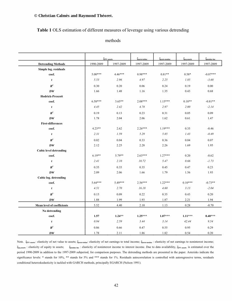
© Christian Calmès and Raymond Théoret.
42
Table 1 OLS estimation of different measures of leverage using various detrending
methods
ξNV-assets ξearn-totinc ξearn-noninc ξeq-assets ξnoninc-inc
Detrending Methods 1990-2009 1997-2009 1997-2009 1997-2009 1997-2009 1997-2009
Simple log. residuals
coef. 5.00*** 4.46*** 0.98*** 0.81** 0.58* -0.87***
t 5.53 2.96 4.97 2.25 1.85 -3.68
R2 0.30 0.20 0.06 0.24 0.19 0.00
DW 1.66 1.48 1.16 1.35 0.43 0.68
Hodrick-Prescott
coef. 6.58*** 3.65** 2.08*** 1.15*** 0.18** -0.81**
t 4.45 2.42 4.78 2.97 2.00 -2.14
R2 0.19 0.13 0.23 0.31 0.05 0.09
DW 1.78 2.04 2.06 1.62 0.61 1.47
First-differences
coef. 4.23** 2.62 2.26*** 1.19*** 0.35 -0.46
t 2.31 1.59 5.29 5.85 1.43 -0.49
R2 0.02 0.04 0.33 0.36 0.04 0.07
DW 2.12 2.25 2.28 2.26 1.69 1.95
Cubic level detrending
coef. 6.19** 5.79** 2.63*** 1.27*** 0.20 -0.62
t 2.41 2.10 10.72 5.47 0.66 -1.73
R2 0.35 0.35 0.35 0.45 0.47 0.23
DW 2.09 2.06 1.66 1.79 1.56 1.93
Cubic log. detrending
coef. 5.64*** 5.49*** 2.56*** 1.22*** 0.10*** -0.73**
t 4.51 2.70 16.18 4.60 3.13 -2.04
R2 0.15 0.09 0.22 0.35 0.43 0.20
DW 1.88 1.99 1.93 1.87 2.21 1.94
Mean level of coefficients 5.52 4.40 2.10 1.13 0.28 -0.70
No detrending
coef. 1.57 1.24** 1.25*** 1.07*** 1.11*** 0.40***
t 0.94 2.59 3.44 3.14 42.44 9.54
R2 0.86 0.66 0.47 0.55 0.95 0.29
DW 1.78 2.11 1.86 1.82 0.54 0.20
Note. ξNV-assets : elasticity of net value to assets; ξearn-totinc: elasticity of net earnings to total income; ξearn-noninc : elasticity of net earnings to noninterest income;
ξeq-assets : elasticity of equity to assets; ξnoninc-inc : elasticity of noninterest income to interest income. Due to data availability, ξNV-assets is estimated over the
period 1990-2009 in addition to the 1997-2009 subperiod, for comparison purposes. The detrending methods are presented in the paper. Asterisks indicate the
significance levels: * stands for 10%, ** stands for 5% and *** stands for 1%. Residuals autocorrelation is controlled with autoregressive terms, residuals
conditional heteroskedasticity is tackled with GARCH methods, principally EGARCH (Nelson 1991).
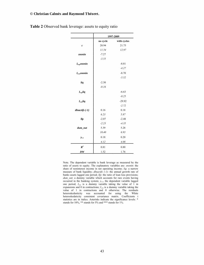
© Christian Calmès and Raymond Théoret.
43
Table 2 Observed bank leverage: assets to equity ratio
1997-2009
no cycle with cycles
c 20.94 21.75
11.54 12.97
snonin -7.27
-3.55
Iexpsnonin -8.81
-4.27
Iconsnonin -8.70
-5.52
liq -2.30
-0.16
Iexpliq -6.63
-0.25
Iconliq -29.92
-2.72
dlnactifs (-1) 0.16 0.18
6.23 5.87
llp -2.07 -2.48
-2.23 -4.35
dum_out 5.39 5.28
10.40 6.93
yt-1 0.18 0.20
4.12 4.08
R2 0.81 0.80
DW 1.52 1.76
Note. The dependent variable is bank leverage as measured by the ratio of assets to equity. The explanatory variables are: snonin: the share of noninterest income in net operating income; liq: a narrow measure of bank liquidity; dlnactifs (-1): the annual growth rate of banks assets lagged one period; llp: the ratio of loan loss provisions; dum_out: a dummy variable which accounts for rare events having occurred in the banking system; yt-1, the dependent variable lagged one period; Iexp is a dummy variable taking the value of 1 in expansions and 0 in contractions; Icon is a dummy variable taking the value of 1 in contractions and 0 otherwise. The residuals heteroskedasticity was accounted for using the White heteroskedaticity consistent covariance matrix. Coefficients t statistics are in italics. Asterisks indicate the significance levels: * stands for 10%, ** stands for 5% and *** stands for 1%.
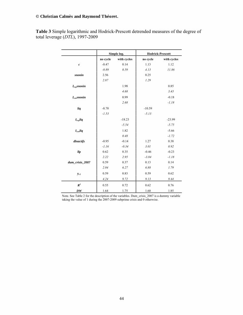
© Christian Calmès and Raymond Théoret.
44
Table 3 Simple logarithmic and Hodrick-Prescott detrended measures of the degree of total leverage (DTL), 1997-2009
Note. See Table 2 for the description of the variables. Dum_crisis_2007 is a dummy variable taking the value of 1 during the 2007-2009 subprime crisis and 0 otherwise.
Simple log. Hodrick-Prescott
no cycle with cycles no cycle with cycles
c -0.47 0.14 1.13 1.12
-0.89 0.59 4.13 11.86
snonin 2.56 0.25
2.87 1.29
Iexpsnonin 1.98 0.85
4.68 3.43
Iconsnonin 0.99 -0.18
2.68 -1.18
liq -8.70 -10.59
-1.53 -5.13
Iexpliq -18.23 -23.99
-5.54 -5.75
Iconliq 1.82 -5.66
0.48 -1.72
dlnactifs -0.95 -0.14 1.27 0.38
-1.16 -0.34 3.01 0.92
llp 0.62 0.35 -0.46 -0.23
2.22 2.95 -3.84 -1.18
dum_crisis_2007 0.59 0.37 0.13 0.14
2.04 6.27 6.88 1.79
yt-1 0.59 0.83 0.59 0.62
4.24 9.72 9.13 9.44
R2 0.55 0.72 0.62 0.76
DW 1.64 1.75 1.60 1.85
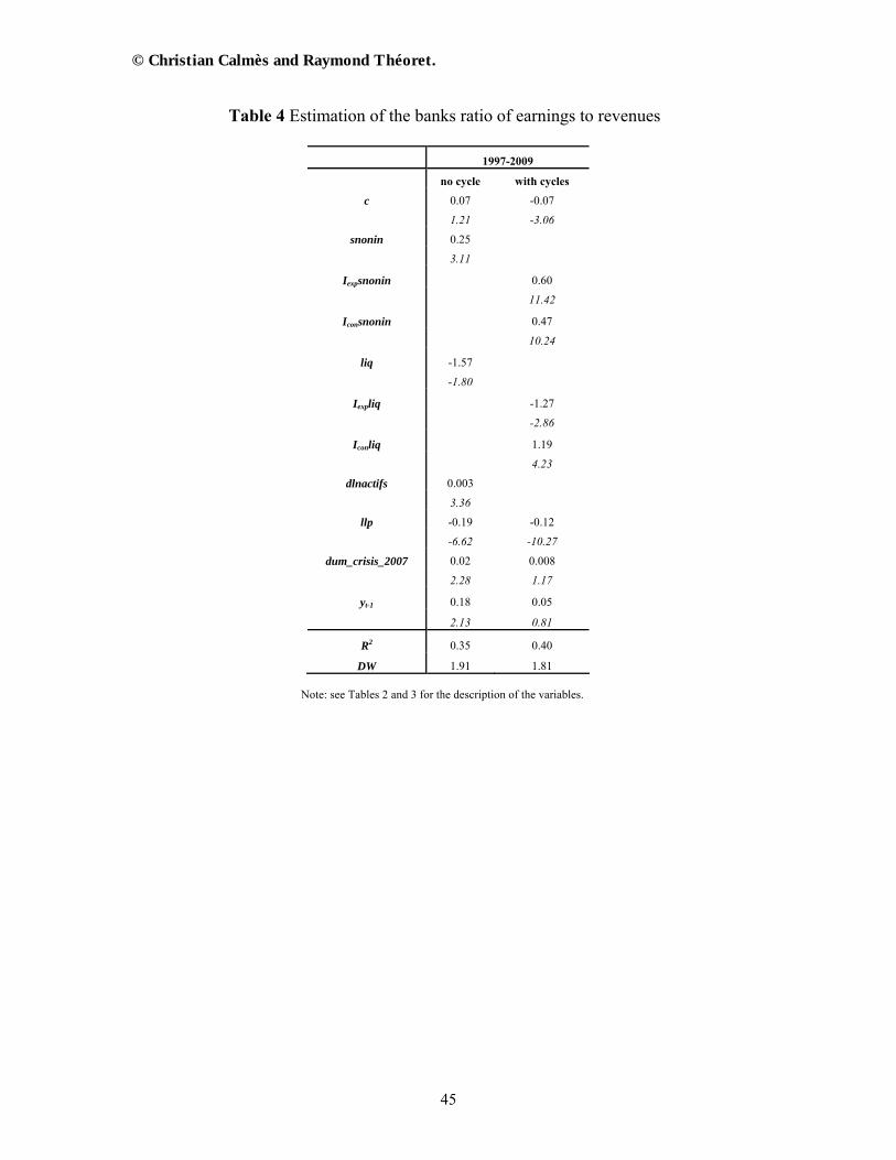
© Christian Calmès and Raymond Théoret.
45
Table 4 Estimation of the banks ratio of earnings to revenues
1997-2009
no cycle with cycles
c 0.07 -0.07
1.21 -3.06
snonin 0.25
3.11
Iexpsnonin 0.60
11.42
Iconsnonin 0.47
10.24
liq -1.57
-1.80
Iexpliq -1.27
-2.86
Iconliq 1.19
4.23
dlnactifs 0.003
3.36
llp -0.19 -0.12
-6.62 -10.27
dum_crisis_2007 0.02 0.008
2.28 1.17
yt-1 0.18 0.05
2.13 0.81
R2 0.35 0.40
DW 1.91 1.81 Note: see Tables 2 and 3 for the description of the variables.
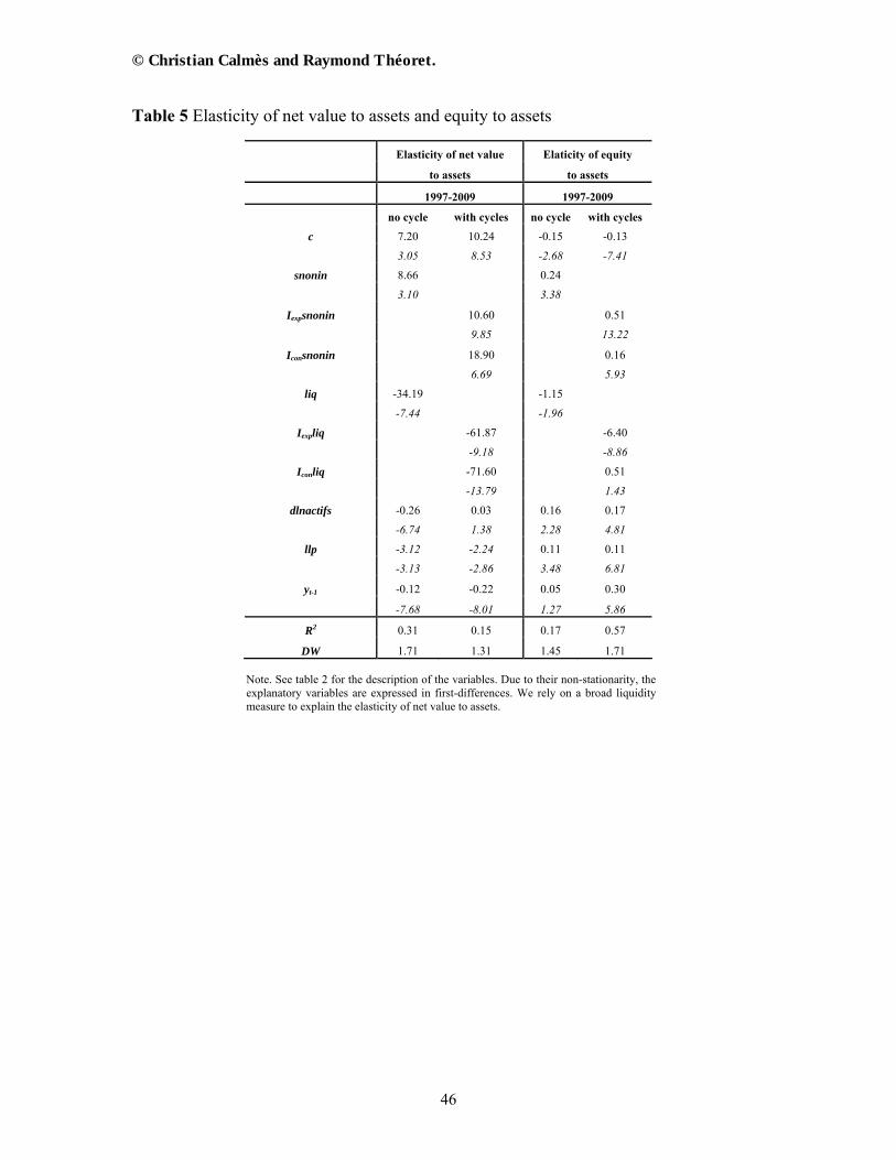
© Christian Calmès and Raymond Théoret.
46
Table 5 Elasticity of net value to assets and equity to assets
Elasticity of net value Elaticity of equity
to assets to assets
1997-2009 1997-2009
no cycle with cycles no cycle with cycles
c 7.20 10.24 -0.15 -0.13
3.05 8.53 -2.68 -7.41
snonin 8.66 0.24
3.10 3.38
Iexpsnonin 10.60 0.51
9.85 13.22
Iconsnonin 18.90 0.16
6.69 5.93
liq -34.19 -1.15
-7.44 -1.96
Iexpliq -61.87 -6.40
-9.18 -8.86
Iconliq -71.60 0.51
-13.79 1.43
dlnactifs -0.26 0.03 0.16 0.17
-6.74 1.38 2.28 4.81
llp -3.12 -2.24 0.11 0.11
-3.13 -2.86 3.48 6.81
yt-1 -0.12 -0.22 0.05 0.30
-7.68 -8.01 1.27 5.86
R2 0.31 0.15 0.17 0.57
DW 1.71 1.31 1.45 1.71
Note. See table 2 for the description of the variables. Due to their non-stationarity, the explanatory variables are expressed in first-differences. We rely on a broad liquidity measure to explain the elasticity of net value to assets.
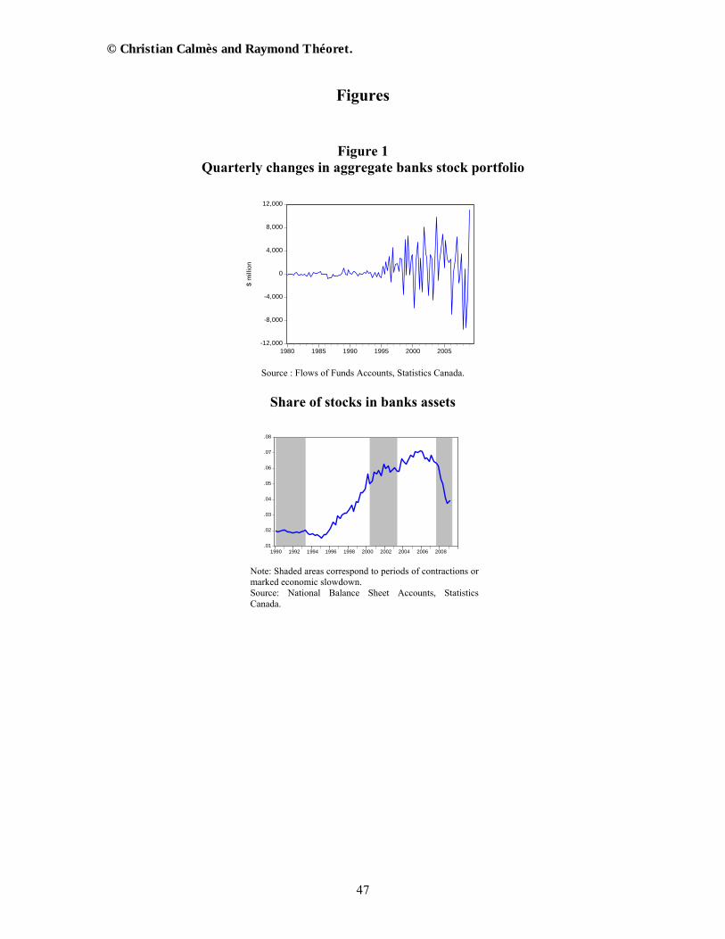
© Christian Calmès and Raymond Théoret.
47
Figures
Figure 1
Quarterly changes in aggregate banks stock portfolio
-12,000
-8,000
-4,000
0
4,000
8,000
12,000
1980 1985 1990 1995 2000 2005
$ m
illio
n
Source : Flows of Funds Accounts, Statistics Canada.
Share of stocks in banks assets
.01
.02
.03
.04
.05
.06
.07
.08
1990 1992 1994 1996 1998 2000 2002 2004 2006 2008
Note: Shaded areas correspond to periods of contractions or marked economic slowdown. Source: National Balance Sheet Accounts, Statistics Canada.

© Christian Calmès and Raymond Théoret.
48
Figure 2 Quarterly changes in banks mortgages
-40,000
-30,000
-20,000
-10,000
0
10,000
20,000
1980 1985 1990 1995 2000 2005
$ m
illio
n
Source : Flows of Funds Accounts, Statistics Canada.
Figure 3 Quarterly changes in banks consumer credit
-12,000
-8,000
-4,000
0
4,000
8,000
12,000
1980 1985 1990 1995 2000 2005
$ m
illio
n
Source : Flows of Funds Accounts, Statistics Canada.
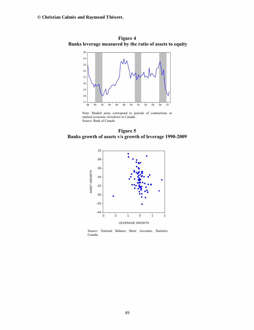
© Christian Calmès and Raymond Théoret.
49
Figure 4
Banks leverage measured by the ratio of assets to equity
17
18
19
20
21
22
23
24
25
88 90 92 94 96 98 00 02 04 06 08 10
Note: Shaded areas correspond to periods of contractions or marked economic slowdown in Canada. Source: Bank of Canada
Figure 5
Banks growth of assets v/s growth of leverage 1990-2009
-.04
-.02
.00
.02
.04
.06
.08
.10
-3 -2 -1 0 1 2
LEVERAGE GROWTH
AS
SE
T G
RO
WT
H
Source: National Balance Sheet Accounts, Statistics Canada.

© Christian Calmès and Raymond Théoret.
50
Figure 6 Short-term paper held by Canadian banks
10,000
20,000
30,000
40,000
50,000
60,000
70,000
80,000
90 92 94 96 98 00 02 04 06 08
$ m
illio
n
Note: Shaded areas correspond to periods of contractions or marked economic slowdown in Canada. Source: National Balance Sheet Accounts, Statistics Canada.
Figure 7 Banks net leverage: (Debt - liquidity) / Assets
.40
.44
.48
.52
.56
.60
.64
.68
97 98 99 00 01 02 03 04 05 06 07 08 09
Note: Shaded areas correspond to periods of contractions or marked economic slowdown in Canada. Source: National Balance Sheet Accounts, Statistics Canada.
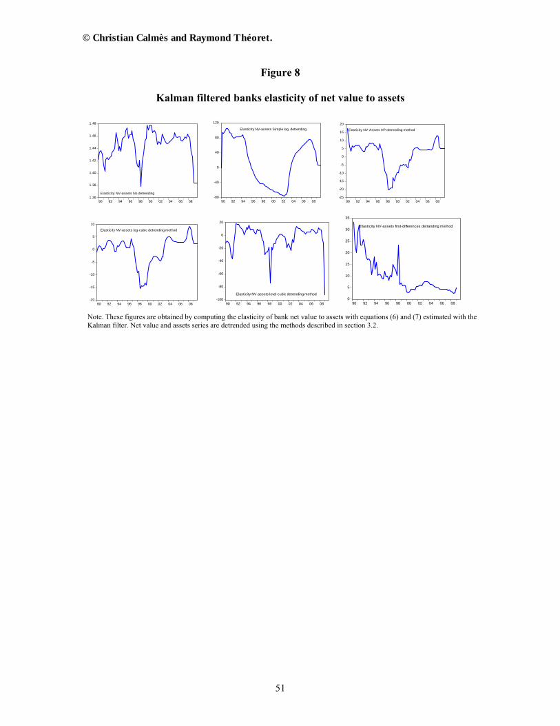
© Christian Calmès and Raymond Théoret.
51
Figure 8
Kalman filtered banks elasticity of net value to assets
1.36
1.38
1.40
1.42
1.44
1.46
1.48
90 92 94 96 98 00 02 04 06 08
Elasticity NV-assets No detrending-80
-40
0
40
80
120
90 92 94 96 98 00 02 04 06 08
Elasticity NV-assets Simple log. detrending
-25
-20
-15
-10
-5
0
5
10
15
20
90 92 94 96 98 00 02 04 06 08
Elasticity NV-Assets HP detrending method
-20
-15
-10
-5
0
5
10
90 92 94 96 98 00 02 04 06 08
Elasticity NV-assets log-cubic detrending method
-100
-80
-60
-40
-20
0
20
90 92 94 96 98 00 02 04 06 08
Elasticity NV-assets level-cubic detrending method0
5
10
15
20
25
30
35
90 92 94 96 98 00 02 04 06 08
Elasticity NV-assets first-differences detranding method
Note. These figures are obtained by computing the elasticity of bank net value to assets with equations (6) and (7) estimated with the Kalman filter. Net value and assets series are detrended using the methods described in section 3.2.
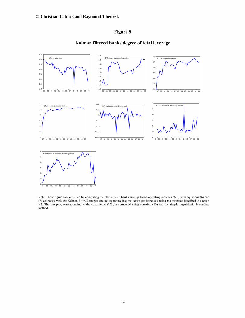
© Christian Calmès and Raymond Théoret.
52
Figure 9
Kalman filtered banks degree of total leverage
2.20
2.24
2.28
2.32
2.36
2.40
2.44
2.48
97 98 99 00 01 02 03 04 05 06 07 08 09
DTL no-detrending
-0.2
0.0
0.2
0.4
0.6
0.8
1.0
1.2
1.4
97 98 99 00 01 02 03 04 05 06 07 08 09
DTL simple log detrending method
0.0
0.5
1.0
1.5
2.0
2.5
3.0
97 98 99 00 01 02 03 04 05 06 07 08 09
DTL HP detrending method
-8
-6
-4
-2
0
2
4
97 98 99 00 01 02 03 04 05 06 07 08 09
DTL log-cubic detrending method
-1,600
-1,200
-800
-400
0
400
800
97 98 99 00 01 02 03 04 05 06 07 08 09
DTL level-cubic detrending method
1
2
3
4
5
6
7
97 98 99 00 01 02 03 04 05 06 07 08 09
DTL first-differences detrending method
0
1
2
3
4
5
6
97 98 99 00 01 02 03 04 05 06 07 08 09
Conditional DTL simple log detrending method
Note. These figures are obtained by computing the elasticity of bank earnings to net operating income (DTL) with equations (6) and (7) estimated with the Kalman filter. Earnings and net operating income series are detrended using the methods described in section 3.2. The last plot, corresponding to the conditional DTL, is computed using equation (10) and the simple logarithmic detrending method.
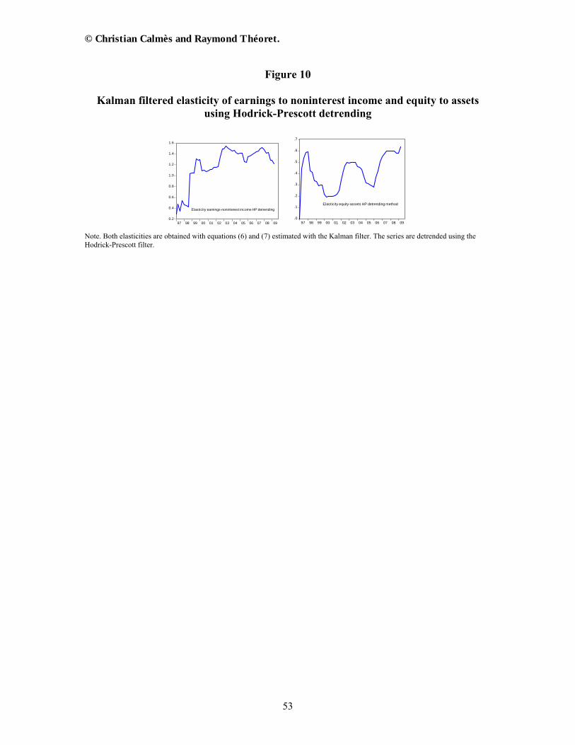
© Christian Calmès and Raymond Théoret.
53
Figure 10
Kalman filtered elasticity of earnings to noninterest income and equity to assets using Hodrick-Prescott detrending
0.2
0.4
0.6
0.8
1.0
1.2
1.4
1.6
97 98 99 00 01 02 03 04 05 06 07 08 09
Elasticity earnings-noninterest income HP detrending
.0
.1
.2
.3
.4
.5
.6
.7
97 98 99 00 01 02 03 04 05 06 07 08 09
Elasticity equity-assets HP detrending method
Note. Both elasticities are obtained with equations (6) and (7) estimated with the Kalman filter. The series are detrended using the Hodrick-Prescott filter.