Achieving Privacy-preserving Distributed Statistical Computation

Achieving Privacy-preserving Distributed

Statistical Computation

A thesis submitted to the University of Manchester

for the degree of Doctor of Philosophy

in the Faculty of Engineering and Physical Sciences

2012

By

Meng-Chang Liu

The School of Computer Science

.

2

Contents…………

CONTENTS…………................................................................................................... 2

LIST OF TABLES ......................................................................................................... 8

LISTS OF FIGURES ................................................................................................... 10

ABBREVIATIONS ..................................................................................................... 14

ABSTRACT…………................................................................................................. 16

DECLARATION……… ............................................................................................. 17

COPYRIGHT AND THE OWNERSHIP OF INTELLECTUAL PROPERTY

RIGHTS ........................................................................................... 18

DEDICATION……… ................................................................................................. 19

ACKNOWLEDGEMENTS ......................................................................................... 20

CHAPTER 1 INTRODUCTION ........................................................................... 21

1.1 DISTRIBUTED STATISTICAL COMPUTATION ...................................... 21

1.2 PRIVACY CONCERNS IN DISTRIBUTED STATISTICAL

COMPUTATION ................................................................................. 21

1.3 RESEARCH MOTIVATION AND CHALLENGES .................................... 23

1.4 RESEARCH AIM AND OBJECTIVES ..................................................... 26

1.5 RESEARCH METHOD ......................................................................... 27

1.6 NOVEL CONTRIBUTIONS ................................................................... 29

1.7 THESIS STRUCTURE .......................................................................... 33

CHAPTER 2 LITERATURE SURVEY: PRIVACY-PRESERVING

DISTRIBUTED DATA COMPUTATION ..................................... 34

3

2.1 CHAPTER INTRODUCTION ................................................................. 34

2.2 TERMINOLOGIES AND DEFINITIONS .................................................. 34

2.2.1 Computation Models ....................................................................... 34

2.2.2 Data Partitioning Models ................................................................ 44

2.2.3 Adversarial Behaviours ................................................................... 47

2.2.4 Data Privacy Definitions Used in Related Works ........................... 49

2.3 PRIVACY-PRESERVING DISTRIBUTED DATA COMPUTATION:

STATE-OF-THE-ART .......................................................................... 50

2.3.1 Secure Multi-party Computation (SMC) ......................................... 51

2.3.2 Privacy-preserving Data Mining (PPDM) ...................................... 59

2.3.3 Privacy-preserving Distributed Statistical Computation

(PPDSC) .......................................................................................... 65

2.4 IDENTIFICATION OF THE RESEARCH GAP .......................................... 74

2.5 THE BEST WAY FORWARD ............................................................... 75

2.6 CHAPTER SUMMARY ........................................................................ 76

CHAPTER 3 DESIGN PRELIMINARIES AND EVALUATION

METHOD ........................................................................................ 77


3.2 DEFINITION OF DATA PRIVACY ........................................................ 77

3.3 THE NST COMPUTATION .................................................................. 79

3.3.1 The NST Computation Problem ...................................................... 81

3.3.2 The TTP-NST Algorithm .................................................................. 81

4

3.4 DESIGN REQUIREMENTS ................................................................... 85

3.5 EVALUATION STRATEGY .................................................................. 87

3.5.1 Correctness ...................................................................................... 87

3.5.2 Level of Security .............................................................................. 88

3.5.3 Computational Overhead ................................................................ 88

3.5.4 Communication Overhead ............................................................... 89

3.5.5 Execution Time ................................................................................ 89

3.6 SIMULATION METHOD ...................................................................... 89

3.6.1 Assumptions ..................................................................................... 89

3.7 CHAPTER SUMMARY ........................................................................ 91

CHAPTER 4 PRIVACY-PRESERVING BUILDING BLOCKS ........................ 92


4.2 DATA PERTURBATION TECHNIQUES ................................................. 92

4.2.1 Data Swapping ................................................................................ 92

4.2.2 Data Randomization ........................................................................ 93

4.2.3 Data Transformation ....................................................................... 95

4.3 CRYPTOGRAPHIC PRIMITIVES ........................................................... 96

4.3.1 Additively Homomorphic Cryptosystem .......................................... 96

4.4 A COMPARISON OF PRIVACY-PRESERVING BUILDING BLOCKS ....... 102

4.5 CHAPTER SUMMARY ...................................................................... 104

5

CHAPTER 5 A NOVEL PRIVACY-PRESERVING TWO-PARTY

NONPARAMETRIC SIGN TEST PROTOCOL SUITE

USING DATA PERTURBATION TECHNIQUES (P22NSTP) ... 105

5.1 CHAPTER INTRODUCTION ............................................................... 105

5.2 OVERVIEW OF THE P22NSTP PROTOCOL SUITE .............................. 105

5.3 THE DESIGN IN DETAIL .................................................................. 108

5.3.1 Computation Participants and Message Objects .......................... 108

5.3.2 Components of the P22NSTP Protocol Suite .................................. 109

5.4 THE P22NSTP PROTOCOL SUITE AND ITS OPERATION .................... 128

5.4.1 Operation of the P22NSTP Protocol Suite ..................................... 128

5.4.2 Correctness .................................................................................... 128

5.4.3 Protocol Analysis .......................................................................... 129

5.5 CHAPTER SUMMARY ...................................................................... 143

CHAPTER 6 A NOVEL PRIVACY-PRESERVING TWO-PARTY

NONPARAMETRIC SIGN TEST PROTOCOL SUITE

USING CRYPTOGRAPHIC PRIMITIVES (P22NSTC) .............. 144


6.2 OVERVIEW OF THE P22NSTC PROTOCOL SUITE .............................. 144

6.3 THE DESIGN IN DETAIL .................................................................. 148

6.3.1 Computation Participants and Message Objects .......................... 148

6.3.2 Components of the P22NSTC Protocol Suite .................................. 150

6.4 THE P22NSTC PROTOCOL SUITE AND ITS OPERATION .................... 154

6.4.1 The Operation ................................................................................ 155

6

6.4.2 Correctness .................................................................................... 158

6.4.3 Protocol Analysis .......................................................................... 159

6.5 CHAPTER SUMMARY ...................................................................... 170

CHAPTER 7 A COMPARISON OF THE TTP-NST, THE P22NSTP AND

THE P22NSTC ............................................................................... 171


7.2 A COMPARISON OF PRIVACY PROTECTION ..................................... 172

7.3 A COMPARISON OF COMPUTATIONAL OVERHEAD .......................... 174

7.4 A COMPARISON OF COMMUNICATION OVERHEAD ......................... 175

7.5 A COMPARISON OF EXECUTION TIME ............................................. 176

7.6 FURTHER DISCUSSIONS .................................................................. 179

7.7 CHAPTER SUMMARY ...................................................................... 181

CHAPTER 8 CONCLUSION AND FUTURE WORK ...................................... 182

8.1 THESIS SUMMARY .......................................................................... 182

8.1.1 Review of the Thesis ...................................................................... 182

8.1.2 Contributions ................................................................................. 184

8.2 FUTURE WORK ............................................................................... 186

REFERENCES………… .......................................................................................... 189

APPENDIX……… .................................................................................................... 209

A. DEFINITIONS OF PRIVACY ............................................................... 209

B. PROTOCOL PROTOTYPES ................................................................. 217

7

(51,731 words)

8

List of Tables

TABLE 1. A COMPARISON OF SOLUTIONS TO THE YMP. .................................. 54

TABLE 2. AN EXAMPLE TABLE OF FREQUENCY COUNT FOR DATA

SUBJECTS WHOSE AGE IS BETWEEN 1 TO 10 AND WHO LIVE IN

AREA A1 TO A4. ......................................................................................... 67

TABLE 3. AN EXAMPLE OF ATTRIBUTE RECODING. .......................................... 67

TABLE 4. AN EXAMPLE OF TOP-RECODING. ........................................................ 68

TABLE 5. A TABLE WITH SENSITIVE CELL (C,B). ................................................ 68

TABLE 6. A TABLE WITH SENSITIVE CELLS SUPPRESSED AND FURTHER

COMPLEMENTARY SUPPRESSION MADE. .......................................... 69

TABLE 7. A TABLE WITH CELL VALUES BEEN RANDOMLY ROUNDED TO A

BASE OF 5. ................................................................................................... 69

TABLE 8. THE ENTROPY VALUES. ........................................................................ 131

TABLE 9. A TABLE OF SAMPLE SIZE VERSUS THE INCREMENTS OF

ENTROPY WHEN THE LEVEL OF NOISE DATA ITEM ADDITION IS

INCREASED. .............................................................................................. 134

TABLE 10. THE ENTROPY VALUE AND THE INCREMENT VERSUS 7k . (K7 = 10,

20, 30, 40, 50, 60, 70, 80, 90, 100.) ............................................................. 136

TABLE 11. THE ENTROPY VALUE AND THE INCREMENT VERSUS 7k . (K7 = 100,

200, 300, 400, 500, 600, 700, 800, 900, 1000.) ........................................... 137

TABLE 12. THE ENTROPY VALUE AND THE INCREMENT VERSUS 7k . (K7 =

1000, 2000, 3000, 4000, 5000, 6000, 7000, 8000, 9000, 10000.) ............... 137

TABLE 13. THE ENTROPY VALUE AND THE INCREMENT VERSUS SAMPLE

SIZE. (SAMPLE SIZE N = 10, 20, 30, 40, 50, 60, 70, 80, 90, 100.) ......... 162

9


SIZE. (SAMPLE SIZE N = 100, 200, 300, 400, 500, 600, 700, 800, 900,

1000.) ........................................................................................................... 162


SIZE. (SAMPLE SIZE N = 1000, 2000, 3000, 4000, 5000, 6000, 7000, 8000,

9000, 10000.) ............................................................................................... 162


SIZE. (SAMPLE SIZE N = 10000, 20000, 30000, 40000, 50000, 60000,

70000, 80000, 90000, 100000.) ................................................................... 162

TABLE 17. THE EXECUTION TIME OF THE TTP-NST, THE P22NSTP AND THE

P22NSTC (SEC). .......................................................................................... 176

TABLE 18. A TABLE OF PROTOCOL EFFICIENCY FOR THE TTP-NST, THE

P22NSTP AND THE P

22NSTC. .................................................................... 177

10

Lists of Figures

FIGURE 1. THE TRUSTED THIRD PARTY (TTP) COMPUTATION MODEL. ........ 35

FIGURE 2. AN EXAMPLE OF THE COMMODITY SERVER MODEL. .................... 37

FIGURE 3. AN EXAMPLE OF THE PROGRAM ISSUER MODEL. ........................... 38

FIGURE 4. AN EXAMPLE OF FAIRNESS CHECKER STTP MODEL. ...................... 39

FIGURE 5. AN EXAMPLE OF THE ON-LINE STTP MODEL. ................................... 40

FIGURE 6. AN EXAMPLE OF THE TWO-PARTY COMPUTATION MODEL. ........ 42

FIGURE 7. AN EXAMPLE OF A N-PARTY COMPUTATION. .................................. 43

FIGURE 8. AN EXAMPLE OF A VERTICALLY PARTITIONED DATA MODEL IN

THE TWO-PARTY COMPUTATION. ........................................................ 45

FIGURE 9. AN EXAMPLE OF A HORIZONTALLY PARTITIONED DATA MODEL

IN THE TWO-PARTY COMPUTATION. ................................................... 46

FIGURE 10. AN EXAMPLE OF THE V2PO DATA MODEL......................................... 47

FIGURE 11. A TAXONOMY OF THE DEVELOPED PPDM ALGORITHMS. ............. 65

FIGURE 12. THE TTP-NST COMPUTATION. ............................................................... 82

FIGURE 13. THE TTP-NST ALGORITHM...................................................................... 84

FIGURE 14. AN EXAMPLE OF DATA SWAPPING OPERATION. ............................. 93

FIGURE 15. AN EXAMPLE OF NOISE VALUE ADDITION RANDOMISATION. .... 94

FIGURE 16. AN EXAMPLE OF NOISE ADDITION RANDOMISATION. ................... 94

FIGURE 17. THE HOMOMORPHIC CRYPTOSYSTEM. ............................................... 99

FIGURE 18. A COMPARISON OF PRIVACY-PRESERVING BUILDING BLOCKS. 102

FIGURE 19. AN OVERVIEW OF THE P22NSTP COMPUTATION. ............................ 107

FIGURE 20. THE RPDFGP ALGORITHM. ................................................................... 110

11

FIGURE 21. THE DOP ALGORITHM............................................................................ 113

FIGURE 22. THE STCP ALGORITHM. ......................................................................... 118

FIGURE 23. THE DEP ALGORITHM. ........................................................................... 124

FIGURE 24. THE DETAILED RELATIONSHIP AMONG iC , Id

ic ANDT

iR . ............. 126

FIGURE 25. THE PRP ALGORITHM. ........................................................................... 127

FIGURE 26. THE P22NSTP PROTOCOL SUITE OPERATION. ................................... 128

FIGURE 27. THE ENTROPY VALUE VERSUS THE NUMBER OF NOISE DATA

ITEMS (N = 10, 20, 30, 40, 50, 60, 70, 80, 90, 100). .................................. 132


ITEMS (N = 10, 100, 1000)......................................................................... 133


ITEMS (N = 1000, 10000, 100000). ............................................................ 133

FIGURE 30. THE ENTROPY VALUE VERSUS THE VALUE OF 7k . (K7 = 10, 20, 30,

40, 50, 60, 70, 80, 90, 100.) ......................................................................... 137

FIGURE 31. THE ENTROPY VALUE VERSUS THE VALUE OF 7k . (K7 = 100, 200,

300, 400, 500, 600, 700, 800, 900, 1000.) ................................................... 138

FIGURE 32. THE ENTROPY VALUE VERSUS THE VALUE OF 7k . (K7 = 1000, 2000,

3000, 4000, 5000, 6000, 7000, 8000, 9000, 10000.) ................................... 138

FIGURE 33. THE ENTROPY VALUE VERSUS THE VALUE OF K7. ........................ 139

FIGURE 34. NUMBER OF COMPUTATIONAL OPERATIONS VS. NUMBER OF

NOISE DATA ITEMS ADDED BY ALICE AND BOB. (SAMPLE SIZE N

= 10, 20, 30.) ................................................................................................ 141

FIGURE 35. TOTAL COMMUNICATION OVERHEAD VS. NUMBER OF NOISE

DATA ITEMS ADDED BY ALICE AND BOB. (SAMPLE SIZE N = 10, 20,

30.) ............................................................................................................... 142

12

FIGURE 36. PROTOCOL SUITE EXECUTION TIME VS. NUMBER OF NOISE DATA

ITEMS ADDED BY ALICE AND BOB. (SAMPLE SIZE N = 10, 20, 30.)

143

FIGURE 37. AN OVERVIEW OF THE P22NSTC COMPUTATION. ............................ 148

FIGURE 38. THE DSP ALGORITHM. ........................................................................... 151

FIGURE 39. THE DRP ALGORITHM. ........................................................................... 152

FIGURE 40. THE P22NSTC ALGORITHM. .................................................................... 156

FIGURE 41. THE ENTROPY VALUE VERSUS SAMPLE SIZE. (SAMPLE SIZE N = 10,

20, 30, 40, 50, 60, 70, 80, 90, 100.) ............................................................. 163

FIGURE 42. THE ENTROPY VALUE VERSUS SAMPLE SIZE. (SAMPLE SIZE N =

100, 200, 300, 400, 500, 600, 700, 800, 900, 1000.) ................................... 163


1000, 2000, 3000, 4000, 5000, 6000, 7000, 8000, 9000, 10000.) ............... 164


10000, 20000, 30000, 40000, 50000, 60000, 70000, 80000, 90000, 100000.)

164

FIGURE 45. THE ENTROPY VALUE VERSUS SAMPLE SIZE. (OVERVIEW) ....... 165

FIGURE 46. COMPUTATIONAL OVERHEAD FOR NON-CRYPTOGRAPHIC

OPERATIONS AND CRYPTOGRAPHIC OPERATIONS VS. NUMBER

OF NOISE DATA ITEMS ADDED BY THE STTP FOR ALICE AND BOB,

RESPECTIVELY. (SAMPLE SIZE N = 10, 20, 30, 40, 50, 60, 70, 80, 90,

100, 200, 300, 400, 500, 600, 700.) ............................................................. 166

FIGURE 47. COMPUTATIONAL OVERHEAD FOR NON-CRYPTOGRAPHIC

OPERATIONS AND CRYPTOGRAPHIC OPERATIONS VS. NUMBER

OF NOISE DATA ITEMS ADDED BY THE STTP. (SAMPLE SIZE N = 10,

20, 30, 40, 50, 60, 70, 80, 90, 100, 200, 300, 400, 500, 600, 700.) ............. 166

FIGURE 48. COMMUNICATION OVERHEAD FOR NON-ENCRYPTED DATA

ITEMS AND ENCRYPTED DATA ITEMS VS. NUMBER OF NOISE

DATA ITEMS ADDED BY THE STTP FOR ALICE AND BOB,

13

RESPECTIVELY. (SAMPLE SIZE N = 10, 20, 30, 40, 50, 60, 70, 80, 90,

100, 200, 300, 400, 500, 600, 700.) ............................................................. 168

FIGURE 49. COMMUNICATION OVERHEAD FOR NON-ENCRYPTED DATA

ITEMS AND ENCRYPTED DATA ITEMS VS. NUMBER OF NOISE

DATA ITEMS ADDED BY THE STTP. (SAMPLE SIZE N = 10, 20, 30, 40,

50, 60, 70, 80, 90, 100, 200, 300, 400, 500, 600, 700.) ............................... 168


ITEMS ADDED BY THE STTP FOR ALICE AND BOB. (SAMPLE SIZE

N = 10, 20, 30, 40, 50, 60, 70, 80, 90, 100, 200, 300, 400, 500, 600, 700.) 169


ITEMS ADDED BY THE STTP. (SAMPLE SIZE N = 10, 20, 30, 40, 50, 60,

70, 80, 90, 100, 200, 300, 400, 500, 600, 700.) ........................................... 169

FIGURE 52. A COMPARISON OF PRIVACY PROTECTION BY THE TTP-NST, THE

P22NSTP AND THE P

22NSTC. .................................................................... 172

FIGURE 53. A COMPARISON OF COMPUTATION OVERHEAD. ........................... 174

FIGURE 54. A COMPARISON OF COMMUNICATION OVERHEAD ...................... 175

FIGURE 55. A COMPARISON OF EXECUTION TIME FOR THE TTP-NST, THE

P22NSTP AND THE P

22NSTC (SEC). ......................................................... 176

FIGURE 56. A COMPARISON OF PROTOCOL EFFICIENCY FOR THE TTP-NST,

THE P22NSTP AND THE P

22NSTC. ........................................................... 177

14

Abbreviations

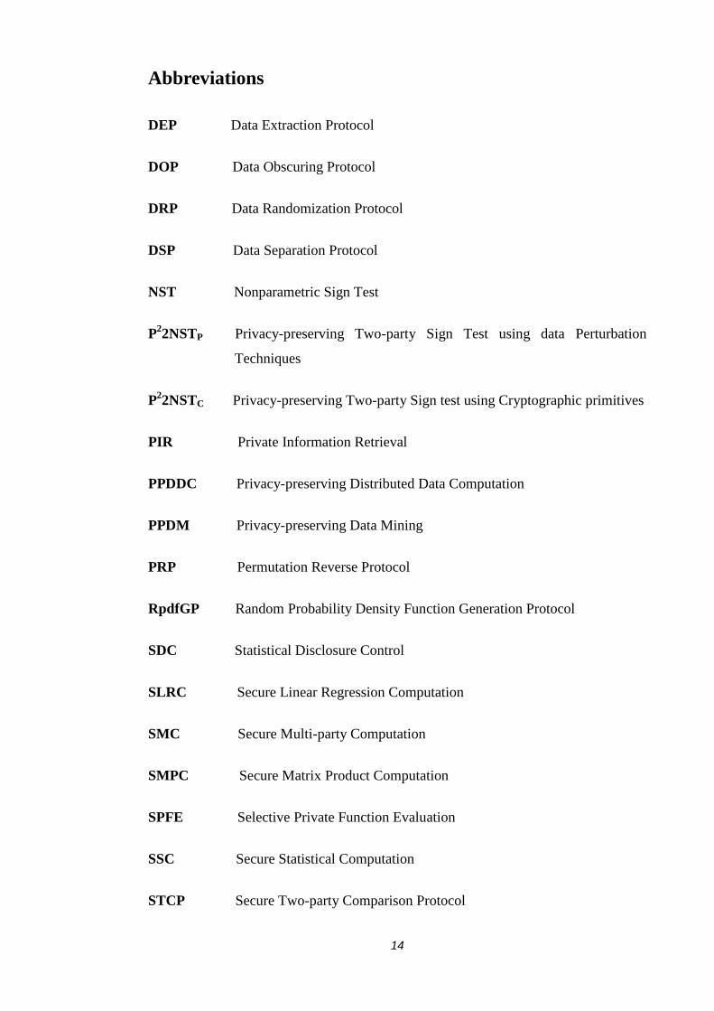
DEP Data Extraction Protocol

DOP Data Obscuring Protocol

DRP Data Randomization Protocol

DSP Data Separation Protocol

NST Nonparametric Sign Test

P22NSTP Privacy-preserving Two-party Sign Test using data Perturbation

Techniques

P22NSTC Privacy-preserving Two-party Sign test using Cryptographic primitives

PIR Private Information Retrieval

PPDDC Privacy-preserving Distributed Data Computation

PPDM Privacy-preserving Data Mining

PRP Permutation Reverse Protocol

RpdfGP Random Probability Density Function Generation Protocol

SDC Statistical Disclosure Control

SLRC Secure Linear Regression Computation

SMC Secure Multi-party Computation

SMPC Secure Matrix Product Computation

SPFE Selective Private Function Evaluation

SSC Secure Statistical Computation

STCP Secure Two-party Comparison Protocol

15

STTP Semi-trusted Third Party

TP Third Party

TTP Trusted Third Party

TTP-NST TTP-based Nonparametric Sign Test Computation

YMP Yao’s Millionaires’ Problem

16

Abstract…………

Name of the University: University of Manchester

The Candidate’s full name: Meng-chang Liu

Degree Title: Doctor of Philosophy

Thesis Title: Achieving Privacy-preserving Distributed Statistical Computation

Date: 30 September 2011

The growth of the Internet has opened up tremendous opportunities for cooperative

computations where the results depend on the private data inputs of distributed

participating parties. In most cases, such computations are performed by multiple

mutually untrusting parties. This has led the research community into studying

methods for performing computation across the Internet securely and efficiently.

This thesis investigates security methods in the search for an optimum solution to

privacy- preserving distributed statistical computation problems. For this purpose, the

nonparametric sign test algorithm is chosen as a case for study to demonstrate our

research methodology. Two privacy-preserving protocol suites using data perturbation

techniques and cryptographic primitives are designed. The first protocol suite, i.e. the

P22NSTP, is based on five novel data perturbation building blocks, i.e. the random

probability density function generation protocol (RpdfGP), the data obscuring

protocol (DOP), the secure two-party comparison protocol (STCP), the data extraction

protocol (DEP) and the permutation reverse protocol (PRP). This protocol suite

enables two parties to efficiently and securely perform the sign test computation

without the use of a third party. The second protocol suite, i.e. the P22NSTC, uses an

additively homomorphic encryption scheme and two novel building blocks, i.e. the

data separation protocol (DSP) and data randomization protocol (DRP). With some

assistance from an on-line STTP, this protocol suite provides an alternative solution

for two parties to achieve a secure privacy-preserving nonparametric sign test

computation. These two protocol suites have been implemented using MATLAB

software. Their implementations are evaluated and compared against the sign test

computation algorithm on an ideal trusted third party model (TTP-NST) in terms of

security, computation and communication overheads and protocol execution times.

By managing the level of noise data item addition, the P22NSTP can achieve specific

levels of privacy protection to fit particular computation scenarios. Alternatively, the

P22NSTC provides a more secure solution than the P

22NSTP by employing an on-line

STTP. The level of privacy protection relies on the use of an additively homomorphic

encryption scheme, DSP and DRP. A four-phase privacy-preserving transformation

methodology has also been demonstrated; it includes data privacy definition,

statistical algorithm decomposition, solution design and solution implementation.

17

Declaration………

No portion of the work referred to in the thesis has been submitted in support of an

application for another degree or qualification of this or any other university or other

institute of learning

Signed………………………………………………………………………………….

18

Copyright and the Ownership of Intellectual Property

Rights

i. Copyright in text of this thesis rests with the Author. Copies (by any process)

either in full, or of extracts, may be made only in accordance with instructions

given by the Author and lodged in the John Ryland’s University Library of

Manchester. Details of may be obtained form the Librarian. This page must form

part of any such copies made. Further copies (by any process) of copies made in

accordance with such instructions may not be made without the permission (in

writing) of the Author.

ii. The ownership of any intellectual property rights which may be described in this

thesis is vested in the University of Manchester, subject to any prior agreement to

the contrary, and may not be made available for use by third parties without the

written permission of the University, which will prescribe the terms and

conditions of any such agreement.

iii. Further information on the conditions under which disclosures and exploitation

may take place is available form the Head of the School of Computer Science.

19

Dedication………

To my family.

20

Acknowledgements

I would like to express my sincerest gratitude to my supervisor, Dr. Ning Zhang, for

her guidance and valuable advice throughout this PhD research.

I would also like to thank my friends and colleagues, Namshik and Kits, for the

valuable discussion about the simulation.

21

Chapter 1 Introduction

1.1 Distributed Statistical Computation

With the advancement of computer and internet technologies, organizations and

individuals are now able to collect and store a great amount of data for research or

business purposes. Consequently, the more records are collected the more valuable

information in the data. Applications of statistical data analysis techniques have

hugely improved the utility of these data for such purposes. Using specified

techniques, the trend or statistical properties of a dataset can easily be computed from

the raw data. Data holders are then able to reveal specialized information from the

computation results. For example, to analyze the 1900-1950 temperature records in

the Arctic using a statistical hypothesis test technique, the hypothesis of the rising

average Arctic temperature can be tested and uncovered, and factors affecting global

warming in the Arctic can be identified. Researchers then may be able to investigate

more efficient ways to address the global warming problem. In many cases, more

reliable and useful information can be learnt from datasets contributed by multiple

data holders. For example, Russia, Norway, the Unites States, Canada and Denmark

each own part of the Arctic. They each hold the regional temperature records of the

Arctic. The information uncovered from one country’s database can not be used to

represent the actual situation of the whole Arctic. If all the five countries can share

their temperature records with one another and perform statistical hypothesis tests

collaboratively, this information may bring to light more truth about the actual

situation in the Arctic than the results based on regional data. In other words, more

accurately analysed results require the use of more comprehensive datasets, and in

many cases, datasets are managed by different data holders. A distributed statistical

computation method that supports multiple parties to collaboratively compute on their

joint dataset would be an ideal solution.

1.2 Privacy Concerns in Distributed Statistical Computation

Distributed statistical computation, however, raises privacy concerns among data

holders (e.g. data providers) as well as data owners (i.e. data subjects) [CLIF’02b].

Privacy is the right of individuals to determine for themselves when, how and to what

22

extent information about them is communicated to others. Information in this context

concerns not only the raw data about an individual (e.g. name, age and sex), but also

their credentials (e.g. degree certificate and invalidity benefit entitlement) and their

policies (e.g. I never tell anyone my annual income). The data owners are data

subjects that submit their private data items to data providers while the data providers

are individuals or organizations that collect data and manage data repositories. In

other words, data providers are third parties managing and using data provided by

data owners. One of the key issues in protecting a data subject’s privacy by its data

holder is how to manage the identifiable information so that the data released for other

purposes does not violate the data subject’s wishes (i.e. privacy policies). The

European Community regulation [DIRE’95] and U.S.HIPAA rules [OCR’03] are

regulations to govern data providers, i.e. they are held legally responsible for making

sure that data under their management are protected properly. In addition, data owners

also have privacy concerns regarding whether data providers would use their data for

purposes that are different from what their data are submitted for. These concerns, if

not addressed properly, will deter their willingness to submit their data to data

providers.

Concerted research efforts have been made to search for ways to achieve privacy-

preserving collaborative computation. These efforts can largely be divided into two

categories:

Anonymising the data (i.e. removing all information that can directly link data

items to their owners) so that it can not be traced to the identity of the subject

[SAMA’98, SWEE’02a, WU’06]. There are two problems associated with this

approach. The first problem is that there is a fine balance between the

usefulness of the data and the degree of anonymisation. A high degree of

anonymisation resulting in a high level of privacy protection often means that

the resulting data is useless. Secondly, anonymising the data could make re-

identification of the data subject impossible. However, such re-identification is

necessary for applications such as health care: simply removing one’s

identifying information may not be sufficient to protect his/her privacy. There

are examples showing that even if the identity related information is removed

from the released data, combining the data with other available information

23

sources or knowledge may still expose the identity of the data subject

[CAST’10].

Making use of cryptographic primitives and/or other data perturbation

techniques to preserve data privacy while supporting distributed computation.

This category is sometimes also referred to as secure multiparty computation

(SMC) [DU’01b, DU’01c, GOLD’04]. When a function is computed on a joint

dataset containing data inputs from multiple parties, cryptographic primitives

and/or other privacy-preserving techniques are employed to ensure that no

more information is revealed to a participating party other than the final

computational result. For example, privacy-preserving data mining (PPDM)

and privacy-preserving distributed statistical computation [PPDSC]. PPDM

focuses on transforming normal data mining computation algorithms to

privacy-preserving ones by using both cryptographic primitives and data

perturbation techniques [AGRA’00, AGRA’01, AGGA’08a]. PPDSC can be

further divided into two subcategories: statistical disclosure control (SDC) and

secure statistical computation (SSC). On the one hand, SDC methods are

mainly related to the data dissemination stage and are usually based on

restricting the amount of or modifying the data released [WILL’96, WILL’01].

They are normally applied to two types of data: Microdata and Tabular Data.

Microdata consists of individual statistical records relating to a single

statistical unit. Tabular data is the aggregated information on entities presented

in tables. On the other hand, SSC solutions provide privacy-preserving

algorithms to address privacy concerns when multiple parties perform

statistical computation on the joint dataset [LUO’03, DU’04, KARR’09b].

1.3 Research Motivation and Challenges

Early solutions to the privacy-preserving distributed data computation (PPDDC)

problems [GOLD’87, YAO’87, GOLD’98, GOLD’04] take a generic approach: a

computational problem is firstly described as a combinatorial circuit. The

computation participating parties generate a simple protocol for every gate of this

circuit, respectively. These protocols are then executed during the circuit execution.

Almost all PPDDC problems can be solved by using this approach, which is appealing

because of its generality and simplicity. However, it is neither efficient nor practical

for many research problems. As indicated by Goldreich et al in [GOLD’98,

24

GOLD’04], applying solutions derived from general results to specific cases of SMC

problems can be impractical, and it is preferable that specific solutions are developed

for specific SMC problems in order to devise more efficient solutions suited to

different application contexts. Accordingly, later solutions have been mostly designed

to tackle specific data computation problems. To date little effort has been expended

on designing privacy-preserving solutions to support distributed statistical

computations [DU’01c]. As mentioned by Goldwasser regarding the importance of

this research field [GOLD’97]: “the field of multi-party computation is today where

public-key cryptography was ten years ago, namely, an extremely powerful tool and

rich theory whose real-life usage is at this time only beginning but will become in the

future an integral part of our computing reality”.

Motivated by these observations, this thesis focuses on the study, research and

development of an efficient and practical solution to the privacy-preserving

distributed statistical computation (PPDSC) problem. The two-party nonparametric

sign test computation (P22NST) problem is chosen as a case for study. Two novel

protocol suites have been developed, namely, the privacy-preserving two-party sign

test protocol suite using data perturbation techniques (P22NSTP) and the privacy-

preserving two-party sign test protocol suite using cryptographic primitives

(P22NSTC). In designing these protocols, the following challenges have been

addressed:

The Definition of Data Privacy

A specific computation problem involves a specific type of dataset which

associates with particular type of data privacy. Prior to investigating and

designing solutions to the P22NST problem, it is necessary to clarify the

definition of data privacy in the PPDSC context.

The Identification of Potential Security Threats in the Context of the

P22NST Computation

It is critical that a secure P22NST protocol should not only protect data privacy

but also allow the computation to be carried out. In other words, it should

protect data privacy against security threats throughout the entirety of the

computation. For this purpose, the sign test computation algorithm on an ideal

25

trusted third party model (TTP-NST) is decomposed and threats to data

privacy at each step of the computation have been analysed and identified.

The Identification of Appropriate Privacy-preserving Primitives to

Counter Threats to Data Privacy in the P22NST Computation

There are different privacy-preserving primitives each with varying levels of

effectiveness and efficiency. Work has been carried out to identify and

critically analyse various privacy-preserving primitives with the aim of

identifying the most appropriate ones to support our purpose. Two types of

techniques are considered, namely the data perturbation techniques and the

cryptographic primitives. Often there is a trade-off between costs and the

effectiveness of a primitive in protecting data privacy. Acceptable trade-offs

may need to be made between privacy protection and performance

(computational and communicational) efficiency in designing a P22NST

solution in order to achieve a cost-effective and practical solution to the

P22NST problem.

The Design of Efficient and Practical Protocol Suites to the P22NST

Problem

Two computation models have been investigated, namely the two-party model

and the Semi-trusted Third Party (STTP) model. Based on these computation

models and identified privacy-preserving primitives, two protocol suites have

been designed to support the P22NST computation. In these designs, two data

partitioning models are considered: one is the vertically partitioned

(heterogeneous) model and the other is the horizontally partitioned

(homogeneous) model. Data perturbation techniques and cryptographic

primitives have been used in these protocol suite designs.

The Prototype of the Two Protocol Suites Using MATLAB

The two designed protocol suites, i.e. the P22NSTP and the P

22NSTC protocol

suites, have been prototyped and implemented using MATLAB software. A

set of experiments have been planned and carried out. The performances of the

two protocol suites have been evaluated using these experimental results. A

26

comparison between these two protocol suites against the TTP-NST model has

also been made to identify the features of each protocol suite.

The Development of A Systematic Methodology to the P2DSC

Computation

Through the process of designing solutions to the P22NST problem, a

systematic methodology has been developed in search of an efficient and

practical solution. This approach incorporates privacy definition, statistical

algorithm decomposition, solution design and solution implementation. It has

been demonstrated that this methodology can be used to design solutions to

the P22NST problem. It can also be used to address other PPDSC problems.

1.4 Research Aim and Objectives

The aim of this research is to search for an optimum solution to the PPDSC problems.

For this purpose, the P22NST computation is chosen as a case for study. The

methodology is demonstrated through the process of designing efficient and practical

solutions to the P22NST problem. That is, to design, prototype and evaluate solutions

that take into account not only data privacy but also other attributes, such as

computational and communication overheads, execution time and the trade-off

between efficiency and privacy. To accomplish this aim, the following objectives

have been fulfilled:

1. To study the literature: to critically analyse related works in the topic area and

to identify research gaps to be addressed in this thesis.

2. To specify requirements for preserving data privacy while supporting the

distributed computations. The requirements are aimed at minimizing any

privacy disclosure from data inputs while optimising performance.

3. To investigate and critically analyse state-of-the-art privacy-preserving

primitives and building blocks in PPDDC and identify those that best satisfy

the requirements identified in 2.

4. To design the P22NST protocol suites based on the primitives and building

blocks identified in 3. The design should take into account different data

partitioning models and computational approaches.

5. To prototype the designed protocol suites.

27

6. To informally analyze the security strength of the designed protocol suites

against design requirements.

7. To evaluate the privacy levels, computational and communication overheads

and execution times of the designed protocol suites.

8. To publish research results and write up the PhD thesis.

1.5 Research Method

The four major tasks of this research together with their respective methods of

execution are described below.

Task 1: Literature Review

The first task was to study the area of secure distributed computation. The focus at

this stage was to critically analyse related work in this field and to identify research

gaps or areas where novel contribution could be made. At the end of the literature

review stage, the PPDSC problem was pinpointed as a topic for future work. More

specifically, the privacy-preserving distributed nonparametric sign test (P2DNST)

computation problem was selected as the case for study. Then further literature study

was carried out in the search for an effective and efficient approach to the P2DNST

problem. During the research it became apparent that a new definition of privacy was

needed. This led to the definition of the three-level data privacy definition: individual

data confidentiality, individual privacy and corporate privacy.

Task 2: Theoretical Work

Following the definition of data privacy, the algorithm of nonparametric sign test

(NST) was analysed in a distributed computational context. More specifically, it was

analysed under three different settings: trusted third-party (TTP)-based, semi-trusted

third-party (STTP)-based and two-party/multi-party-based, so as to identify potential

ways of compromising privacy in the computation process. These analyses were

carried out under the assumption of the vertically partitioned data model and the

horizontally partitioned data model. Such analyses led to the decomposition of the

TTP-NST algorithm and the identification of local and global computational tasks and

message exchanges needed to accomplish the global computational task. Then, a set

of design requirements were specified to govern the conversion of NST into privacy-

28

preserving NST. Based on the design requirements, more literature research was

carried out investigating the building blocks that could be used to preserve privacy in

distributed sign test computation. This in turn led to the identification of a set of

building blocks satisfying our design requirements, which were used to secure the

input and output of local computations. At the end of this stage, two novel protocol

suites were designed: the Privacy-preserving Two-party Nonparametric Sign Test

Using Data Perturbation Techniques protocol suite (P22NSTP) and the Privacy-

preserving Two-party Nonparametric Sign Test Using Data Cryptographic

Primitives protocol suite (P22NSTC). The review and study of relevant literature were

continued throughout the whole research period, thus enabling the repeated

refinement of ideas by taking merits from existing works. As the designs of the two

protocol suites were published [LIU’10, LIU’11a, LIU’11b], the comments from

referees were also taken into account to further refine this work.

Task 3: Protocol Implementation

On completion of the theoretical work stage, the next step was to implement and

simulate the proposed protocol suites. The implementation and simulation were

carried out using MATLAB software. Before implementation, it was necessary to be

familiarised with the features of this software in order to use its power to the full

potential. Following this, the protocol suites were implemented. To obtain a correct

simulation result, it was necessary to validate the implementation to ensure the

practical outcome was in line with the theoretical design. This was done by simulation

validation. The validation was performed by deriving a mathematical model of a

simplified simulation model and comparing the simulated results with the results

obtained from the mathematical model. Once the validation was completed, the

simulation model could be run with full confidence. The simulation was run in a set of

scenarios and settings to show that the models are practical and applicable to various

computational scenarios and different data and privacy requirements. The simulation

results were recorded and used to analyse the performance of the protocol suites.

Task 4: Evaluation

To evaluate the performance of the protocol suites, results from the simulation were

plotted into graphs, these graphs which in turns were used to compare the

performances of the proposed protocol suites with that of the TTP-NST model.

29

Conclusions of this research were then drawn from this evaluation. A direction for

future work was also identified from the evaluation.

1.6 Novel Contributions

This research has developed a systematic methodology in the search for an optimum

solution to the PPDSC problems. More specifically, it has designed two protocol

suites to address the P22NST computation problem. To the best of the author’s

knowledge, this is the first work in this area to address privacy-preserving statistical

hypothesis testing (P2SHT) problems in a distributed setting. This research work has

made three significant contributions to the knowledge area. The first contribution is

the design, analysis and evaluation of a two-party based protocol suite to allow two

parties to perform nonparametric sign testing with privacy preservation, i.e. the

P22NSTP protocol suite. The P

22NSTP protocol suite makes use of five novel data

disguising protocols to assist the computation. The second contribution is the design,

analysis and evaluation of an on-line STTP based protocol suite to support privacy-

preserving nonparametric sign test computation, i.e. the P22NSTC protocol suite. This

protocol suite makes use of three cryptographic primitives and a STTP, which only

plays an assistant role in facilitating the computation. The P22NSTC protocol suite is

more secure but less efficient than the P22NSTP protocol suite as the former employs

cryptographic primitives. Both protocol suites have been implemented and evaluated

using MATLAB. The third contribution is the development of a four-phase

methodology to transform a normal statistical algorithm to a privacy-preserving

distributed one. The four phases include (1) data privacy definition, (2) statistical

algorithm decomposition, (3) solution design and (4) solution implementation. The

detailed novel contributions are further described below.

Design, Analysis and Evaluation of the P22NSTP Protocol Suite

1. Dataset properties are firstly examined in both vertically partitioned and

horizontally partitioned data models. This is necessary in order to identify

potential security threats in the algorithm decomposition stage and to identify

privacy-preserving building blocks in the design stage.

2. Security threats are identified upon the decomposition of the TTP-NST

algorithm in the two-party computation model. The algorithm decomposition

30

divides the TTP-NST algorithm into local and global computational tasks. By

examining the security threats in every computational task, design

requirements are specified.

3. Based on the design requirements, appropriate data perturbation techniques are

chosen and used to design the components of the P22NST protocol suite.

These techniques help to protect data privacy while supporting the execution

of each computation task. The components of the P22NSTP protocol suite, i.e.

five novel data perturbation protocols, are designed to address security threats

with efficiency considerations. The first protocol is used by both parties to

disguise their respective datasets before they perform the joint computation.

The second to the fifth protocols are each used to accomplish a local

computational task in the joint computation while protecting the

confidentiality of intermediate computation results. These five protocols are:

Random Probability Density Function Generation Protocol (RpdfGP). This

protocol allows a participating party to randomly generate a Probability

Density Function based on their original dataset.

Data Obscuring Protocol (DOP). This protocol protects data confidentiality

of an original dataset using data perturbation techniques.

Secure Two-party Comparison Protocol (STCP). This protocol allows one

of the participating parties to privately compare their datasets without

learning the exact values of the other party’s dataset and the comparison

result.

Data Extraction Protocol (DEP). This protocol reverses the results of data

disguising operations performed by DOP.

Permutation Reverse Protocol (PRP). This protocol reverses the results of

data disguising operations performed by STCP.

The design requirements are addressed by the five protocols mentioned above,

which make use of data perturbation techniques, namely data randomization,

data swapping and data transformation. As data perturbation techniques are

generally more computationally efficient than cryptographic primitives, this

protocol suite provides better efficiency than the second protocol suite, i.e. the

P22NSTC protocol suite.

4. The P22NSTP protocol suite is implemented using MATLAB.

31

5. Both security analysis and performance evaluation of the P22NSTP protocol

suite are carried out. The security analysis is performed against the privacy

requirements. The performance evaluation is carried out in terms of

computational costs, communication costs and execution time. These costs are

evaluated through the simulation of the protocol suite implementation. The

results collected from the simulation are compared against theoretical results

from a TTP-NST model. The effects of different data sizes and the degree of

noise addition on the performance of the protocol suite are also evaluated.

Design, Analysis and Evaluation of the P22NSTC Protocol Suites

1. An on-line STTP is employed in the design of this protocol suite in order to

provide a higher level of security than the P22NSTP.

2. This protocol suite consists of two novel protocols which are designed to

address security threats in the P22NST computation. They are:

Dataset Split Protocol (DSP): This protocol allows STTP to randomly

separate a encrypted dataset G to two subsets 1G and 2G where

21 GGG and 21 GG .

Dataset Randomization Protocol (DRP): This protocol allows STTP to

randomly generate a randomized dataset 'G based on encrypted G where

'GG .

The design of this protocol suite makes use of both data perturbation techniques,

namely data randomization, data swapping and data transformation, and a

cryptographic primitive, namely an additively homomorphic encryption scheme.

As cryptographic primitives are more secure and more computational expensive

than data perturbation techniques, the P22NSTC provides an alternative solution

to the P22NSTP. As the datasets are encrypted before being sent to the STTP,

this protocol suite enables the STTP to compute the data inputs without

decrypting them.

3. The P22NSTC suite is implemented using MATLAB.

4. A security analysis and performance evaluation of the P22NSTC protocol suite

are carried out and the results collected from the simulation are further

compared against the results from the TTP-NST model and the P22NSTP

protocol suite. The effects of different data sizes and the degree of noise

32

addition on the performance of the protocols, in terms of computational and

communication costs and protocol execution time, are evaluated.

Development of the Four-phase Methodology to Transform A Normal

Statistical Algorithm to A Privacy-preserving Distributed One

1. According to the demonstrations of the P22NSTP and the P

22NSTC, the

development of a four-phase methodology can be summarized. The four

phases are: (1) privacy definition, (2) statistical algorithm decomposition, (3)

solution design and (4) solution implementation.

2. The privacy definition phase identifies and defines crucial information that is

needed to be protected in a dataset which is involved in a distributed statistical

computation problem.

3. The algorithm decomposition phase decomposes the original statistical

computation into a set of local and global computational tasks so as to identify

every potential threat to data privacy in the tasks.

4. In the solution design phase, the most appropriate privacy-preserving building

blocks are selected and used in the designs of the solution so as to achieve a

privacy-preserving solution to the distributed statistical computation problem.

5. Finally, the solution implementation phase implements and evaluates the

designed solution so as to ensure the outcome is in line with the theoretic

design.

Publications

Conference Publications

1. M.C. Liu and N. Zhang, (2010), “A Solution to Privacy-preserving Two-party

Sign Test on Vertically Partitioned Data (P22NSTv) Using Data Disguising

Techniques”, the Proceedings of the International Conference on Networking

and Information Technology (ICNIT 2010), pages 526-534, Manila,

Philippines, 11-12 June 2010, IEEE Computer Society Press.

2. M.C. Liu and N. Zhang, (2011), “A Cryptographic Solution to Privacy-

preserving Two-party Sign Test Computation on Vertically Partitioned Data”,

the Proceedings of the 2nd

International Conference on Electronics and

Information Engineering (ICEIE2011), Tianjin, China. 9-11 September 2011.

33

Journal Publication

3. M.C. Liu and N. Zhang, (2012), “A Cryptographic Solution to Privacy-

preserving Two-party Sign Test Computation on Vertically Partitioned Data”,

Advanced Material Research, Volume 403-408, Pages 1249 – 1257, Trans

Tech Publications, Switzerland, doi: 10.4028/www.scientific.net/AMR.403-

408.1249.

1.7 Thesis Structure

This thesis is organized as follows. Chapter 2 gives the background information and

critical analysis of related works in the field of PPDDC. The focus is on SMC, PPDM

and PPDSC. Chapter 3 details the design preliminaries and evaluation methods used

for the design and evaluation of the novel protocol suits presented in this thesis.

Chapter 4 presents a list of privacy-preserving building blocks that could be used to

achieve PPDDC. Chapter 5 describes the first novel protocol suite, the P22NSTP,

along with its theoretical privacy analysis and performance evaluation, while the

second novel protocol suite, the P22NSTC, which employs more secure cryptographic

primitives and an on-line STTP, is described in Chapter 6. Chapter 7 presents

simulation studies of the two protocol suites, the P22NSTP and the P

22NSTC, and

further evaluates their performances. The performance results are compared with

those from the TTP-NST model. Finally, Chapter 8 concludes this thesis and

highlights future work.

34

Chapter 2 Literature Survey: Privacy-preserving

Distributed Data Computation

2.1 Chapter Introduction

This chapter presents a literature survey of the related works in the domain of

Privacy-preserving Distributed Data Computation (PPDDC) and is organised as

follows. Section 2.2 offers terminologies and definitions that are used in the domain

of PPDDC. Section 2.3 critically analyses the related works in literature, which have

been categorised into three research areas, namely, secure multi-party computation

(SMC), privacy-preserving data mining (PPDM) and privacy-preserving distributed

statistical computation (PPDSC). Section 2.4 identifies gaps in existing solutions and

suggests areas for future work; finally, this chapter is summarized in section 2.5.

2.2 Terminologies and Definitions

The basic concepts, terminologies and definitions introduced in this section are all

used in the domain of PPDDC. The concepts include computation models, data

partitioning models, adversarial models and privacy definitions which are all

described here.

2.2.1 Computation Models

Different computation models will raise a corresponding variety of security concerns.

For example, in a computation with the support from a third party (TP) it is

sometimes necessary to preserve confidential data from the TP, while in a distributed

computation scenario, this concern does not exist. Based on the literature survey,

three computation models have been employed in the related works. They are the

trusted-third party (TTP) model [GOLD’98, GOLD’01, GOLD’04], the semi-trusted

third party (STTP) model [ABAD’02, CACH’99, EMEK’06, FEIG’94, FRAN’97,

KANT’02, KNAT’03, BEAV’97, BEAV’98, CACH’00, DU’01b, DU’04, NAOR’99]

and the two-party/multi-party distributed computational model [CAST’04, DOLE’91,

DU’01b, DU’04, JAGA’06, ZHAO’05] (i.e. a distributed computation is carried out

without any assistance from a third party). For the sake of convenience and clarity, in

35

this section, the two participating parties will be known as Alice and Bob in the

descriptive examples where Alice holds dataset X and Bob holds dataset Y .

Trusted-third Party (TTP)

The TTP Model (also known as the Ideal Model in the literature) assumes that there

exists a TTP to whom all the participants could surrender their data [GOLD’98,

GOLD’01, GOLD’04]. By using the data from the participating parties, the TTP

performs the computation and then delivers the final computation result to the parties.

As the TTP is assumed to be fully trustworthy, and will not reveal any data other than

the final computation result to the parties, no party can learn anything which is not

inferable from its own input and the final computational result, thus achieving

privacy-preserving computation. This model provides an efficient way to support

collaborative computation while preserving the privacy of the parties’ respective data.

Figure 1 illustrates this two party collaborative computation using the TTP-based

model.

Figure 1. The trusted third party (TTP) computation model. (Source: Author’s own)

In this illustration, Alice sends her own private dataset X to the TTP and Bob sends

his own private dataset Y to the TTP. After receiving X and Y , the TTP performs

the computation ),( YXf and generates the computation result YXR , . Finally, the TTP

sends YXR , to Alice and Bob, respectively. Provided that the communication channels

between the TTP and Alice (or Bob) are secure, no external entities could gain access

to data sent over these channels. In addition, the TTP has to be fully trust-worthy. At

the end of this computation, all Alice knows is her own private dataset X and the

36

final computation result YXR , ; all Bob knows is his own private dataset Y and the

final computation result YXR , .

However, this model suffers from a number of limitations. Firstly, the TTP must be

fully and unconditionally trustworthy, and must not collude with any of the

participating parties [GOLD’98, GOLD’01, GOLD’04]. If any of these conditions is

violated, or should the TTP be compromised, the privacy-preserving property will be

lost. In real life, it may be impractical to always assume the existence of a party that

can be trusted unconditionally by all the participating parties. For example, would an

organization in one country always trust, and/or be willing to surrender its data to an

organization in another country? Secondly, due to legal and ethical concerns

[CLIF’04, EURO’95, OCR’03, MUSE’08], data providers managing private and

sensitive personal information are under legal obligations not to release raw data to an

external party even if this party is fully trustworthy. Furthermore, it is not scalable to

rely on the use of a single party to perform the computation and to achieve privacy.

As computation loads increases the TTP is more prone to be a performance bottleneck.

More importantly, it is also a single point of failure. If the TTP breaks down, the

computation will no longer be possible. For these reasons, this model may not be

appropriate in some application contexts.

Semi-trusted Third Party (STTP)

An alternative model to the TTP model is to employ a STTP to assist the computation

[ABAD’02, CACH’99, EMEK’06, FEIG’94, FRAN’97, KANT’02, KNAT’03,

BEAV’97, BEAV’98, CACH’00, DICR’98, DU’01b, DU’04, NAOR’99]. In this

model, the third party is not expected to be heavily involved in the computation so the

level of trust on the third party is reduced. It is assumed that the third party does not

have access to private data contributed by Alice or Bob, nor does it access

computational results. It is also assumed that the third party does not collude with any

of the participants and that it will execute the protocol correctly. For these reasons, the

third party is called STTP. Depending on the way the STTP assists the computation,

this model can be further classified into two categories: (1) the Off-line STTP based

computation model [BEAV’97, BEAV’98, CACH’00, DICR’98, DU’01b, DU’04,

NAOR’99] and (2) the On-line STTP based computation model [ABAD’02,

CACH’99, EMEK’06, FEIG’94, FRAN’97, KANT’02, KNAT’03].

37

Using an Off-line STTP

In the Off-line STTP based computation model, the STTP does not actually perform

any computational task. It does not have access to input data from any of the

participating parties; rather, it acts as a commodity server, a program issuer or a

fairness checker. When the STTP acts as a commodity server it provides random

noise values to the parties as commodities [BEAV’97, BEAV’98, DICR’98, DU’01b,

DU’04]. The parties then use these random values to disguise their private data items

before sending them to the other parties. Basically, the STTP can generate the random

values off-line independently, and sells them to the parties as commodities. This

commodity server model was first proposed by Beaver in [BEAV’97, BEAV’98] and

then widely used in addressing various SMC problems [DICR’98, DU’01b, DU’04].

Figure 2 further illustrates the operation of this commodity server STTP model.

Figure 2. An example of the commodity server model. (Source: Author’s own)

As shown in green square of the figure, the commodity server first generates random

noise V and W off-line and sends them to Alice and Bob, respectively. Alice and

Bob then use the random noises to disguise their private dataset prior to the joint

38

computation, as shown in the blue square of the figure. The commodity server does

not participate in the joint computation.

The second type of the off-line STTP model, i.e. the program issuer model, is widely

applied in the field of private auction and bidding [DICR’98]. In this context, the

STTP acts as an auction issuer and is responsible for preparing a program that can

privately compute data inputs from bidders and generate an output for an auctioneer.

As the program preparation can be done in advance and independently from the

auctioneers, the issuer needs neither to interact with the auctioneers nor the bidders.

Therefore, the auction issuer is able to provide multiple auction programs to multiple

auctioneers at the same time. Figure 3 illustrates the operation of this program issuer

STTP model.

Figure 3. An example of the program issuer model. (Source: Author’s own)

As shown in the figure, the server first generates a program off-line then sends it to

the auctioneer, who then uses this program to start an auction process. The interested

bidders submit their private bid to the auctioneer. The issuer is not involved in the

auction process.

39

In the third type of off-line STTP model, i.e. the fairness checker [CACH’00], the

STTP is used to ensure fairness for a secure computation. It does not participate in the

computation if the participating parties are honest and if messages are delivered error-

free. This model is widely used in the fair exchange of message and digital contract

signing applications. Figure 4 illustrates the operation of the fairness checker STTP

model.

Figure 4. An example of fairness checker STTP model. (Source: Author’s own)

In this figure, Alice and Bob first perform a joint computation, on the completion of

which Alice has a result V and Bob has a result W . Alice and Bob then send V and

W to the verifier, respectively. The verifier compares V and W , and then returns the

comparison result to Alice and Bob, respectively. In this model, the verifier does not

actively take part in the computation; it only waits for the computation results from

Alice and Bob, and compares the results to make sure they are the same. This

comparison operation can be performed off-line.

40

Using an On-line STTP

On the other hand, in the On-line STTP based computation model [ABAD’02,

CACH’99, EMEK’06, FEIG’94, FRAN’97, KANT’02, KANT’03], the STTP actually

takes part in the computation. Unlike the TTP based and the off-line STTP models,

here Alice and Bob need to disguise (perturb or encrypt) their respective data, X and

Y , by employing privacy-preserving techniques (data perturbation techniques or

cryptographic primitives) before sending them to the STTP [ABAD’02, CACH’99,

EMEK’06, FEIG’94, FRAN’97, KANT’02, KANT’03]. This approach typically only

requires two message transactions per party: one for sending their encrypted data to

the STTP, and the other for fetching the computational result from the STTP once the

computation is completed. However, in the case when encryption schemes are used,

in terms of computational cost it is more expensive than the commodity server STTP

model. Therefore, the cryptographic primitives are not preferable when Alice and Bob

are computationally weak and/or the protocol efficiency is a major requirement.

Figure 5 illustrates the operations of this model which employs a symmetric

cryptosystem.

Figure 5. An example of the on-line STTP model. (Source: Author’s own)

41

In this example, Alice and Bob first negotiate a symmetric encryption scheme

))(),(,( kk DEk prior to the computation, where k is the encryption key, )(kE is the

encryption function and )(kD is the decryption function. Then Alice encrypts X and

sends XE to the STTP; Bob encrypts Y and sends YE to the STTP. After receiving

XE and YE , the STTP computes ),( YXER and sends it to Alice and Bob, respectively.

Finally, Alice and Bob each decrypts ),( YXER and gets YXR , , respectively. As

))(),(,( kk DEk is only known to Alice and Bob, the STTP is unable to decrypt XE

and YE . The privacy of X and Y is kept from the STTP.

Two-party / Multi-party Model

As mentioned earlier in this section, in real life, it may be difficult to find a third party

that could be trusted by all the participating parties. Under such circumstances, the

computation can only be carried out by the participating parties themselves. This

leads to the so called multi-party model. The two-party model is the simplest form of

the multi-party model [CAST’04, DOLE’91, DU’01b, DU’04, JAGA’06, ZHAO’05].

In this model, a computation is divided into local and global computational tasks. On

the one hand, a local computational task is one that can be performed by one party

independently, i.e. without further interaction with the other party. On the other hand,

a global computational task requires the two parties to interact, to exchange data and

to compute collaboratively. An output of a local computational task may be the input

of a global computational task; an output of a global computational task may be the

input of a local computational task or another global computational task. As these

intermediate computational results contain aggregated information of an individual

dataset (i.e. X or Y ) or the joint dataset (i.e. YX ), their privacy should be

preserved. Such privacy is protected by data perturbation techniques or cryptography

primitives in the literature. Figure 6 illustrates an example of the privacy-preserving

two-party computation model.

42

Figure 6. An example of the two-party computation model. (Source: Author’s own)

In this example, Alice holds a dataset X and Bob holds a dataset Y , where

}...,,{ 1 nxxX and }...,,{ 1 nyyY . They want to know the mean value of the joint

dataset YX while Alice is kept from knowing Y and Bob from knowing X . For

this purpose, Alice first generates a random dataset V where }...,,{ 1 nvvV . Alice

then computes VXX ' and sends 'X to Bob. After receiving 'X , Bob computes

the mean value of 'X and Y , i.e. YXr ,' , and then sends YXr ,' to Alice. Finally, Alice

computes YXr , by computing )2

( 1,'

n

vr

n

i i

YX

and then sends YXr , to Bob. At the end

of the computation, neither Alice nor Bob knows the exact data inputs of the other

party’s dataset.

In real life scenarios, a computation may be conducted by more than two parties, i.e.

the so called multi-party computational model. Through the use of computation

decomposition, a multi-party computational task can always be decomposed into a

number of two-party computational tasks. The whole computation can then be seen as

a combination of a series of two-party computational tasks. Therefore, a solution to a

two-party computational problem can easily be extended into a solution to address a

43

multi-party computational problem. Figure 7 illustrates an example of decomposing a

multi-party computational task into a number of two-party computational tasks.

Figure 7. An example of a n-party computation. (Source: Author’s own)

In this example, n parties want to securely compute the sum of their private data

input, but none of them is willing to share their private data inputs with any of the

other parties. Prior to the computation, they have agreed to do this computation using

the following two-phase method: In the first phase, party 1 calculates 1R by adding a

random noise 1r to its private input 1x , then sends 1R to party 2. Then for

)1(...,,2 ni , party i computes iR by calculating iii rxR 1 and sends iR to

party 1i . After receiving 1nR , party n calculates nninn RrxR 1 and sends nR

to party 1. In the second phase, party 1 takes away 1r from nR , i.e. calculating

11 SrRn , and sends 1S to party 2. Then for )1(...,,2 ni , party i takes away ir

from 1iS by calculating iii SrS 1 and sends iS to party 1i . Finally, party n

calculates nnn SrS 1 , where nS equals to

n

i ix1

. Party n then sends nS to all

other parties. By the end of this computation, each party only knows its own private

data input and the final computation result nS , provided that they do not collude with

44

one another. Figure 7 further shows that this multiparty computation can be

decomposed into a number of two-party computation tasks. In this figure, each blue

rectangle represents a two-party computation task. This n -party computation can be

decomposed to )12( n two-party computations.

2.2.2 Data Partitioning Models

In a distributed computation environment, data inputs are contributed from multiple

independent participants (data holders). The joint dataset contributed from different

participants may form different data models, i.e. a vertically partitioned data model

[AGGA’08, DU’01b, DU’01d, DU’04, KARR’09, LIU’10, REIT’04, VAID’02,

VAID’04, VAID’06], a horizontally partitioned data model [AGGA’08, DU’01b,

DU’01d, DU’04, VAID’06] and a hybrid data model [REIT’04]. These data models

play an important role in the design of privacy-preserving distributed computation

algorithms. The properties of these data models are described below.

Vertically Partitioned Data (Heterogeneous Data) Model

In the vertically partitioned data model, all participating parties hold data of the same

group of data subjects (i.e. data owners), but with different data attributes (i.e.

variables) [AGGA’08, DU’01b, DU’01d, DU’04, KARR’09, LIU’10, REIT’04,

VAID’02, VAID’04, VAID’06]. For example, if the joint dataset consists of the data

attributes of weight, height, blood pressure, job, income and tax, then, in the two-

party vertically partitioned data model, participant Alice may hold values of the

attributes of weight, height and blood pressure, while Bob holds the values of the

attributes of job, income and tax. In other words, a vertically partitioned data model

assumes that multiple parties have data collected from the same set of subjects but

each party only possesses data on different sets of attributes. This data model is also

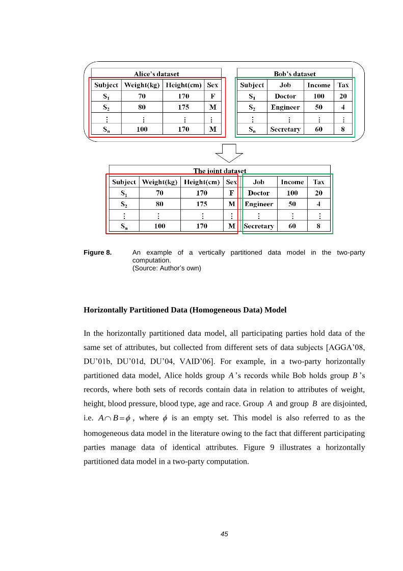
referred to as a heterogeneous data model in the literature. Figure 8 illustrates a

vertically partitioned data model in a two-party computation.

45

Figure 8. An example of a vertically partitioned data model in the two-party computation. (Source: Author’s own)

Horizontally Partitioned Data (Homogeneous Data) Model

In the horizontally partitioned data model, all participating parties hold data of the

same set of attributes, but collected from different sets of data subjects [AGGA’08,

DU’01b, DU’01d, DU’04, VAID’06]. For example, in a two-party horizontally

partitioned data model, Alice holds group A ’s records while Bob holds group B ’s

records, where both sets of records contain data in relation to attributes of weight,

height, blood pressure, blood type, age and race. Group A and group B are disjointed,

i.e. BA , where is an empty set. This model is also referred to as the

homogeneous data model in the literature owing to the fact that different participating

parties manage data of identical attributes. Figure 9 illustrates a horizontally

partitioned data model in a two-party computation.

46

Figure 9. An example of a horizontally partitioned data model in the two-party computation. (Source: Author’s own)

Hybrid Model - Vertically Partitioned, Partial Overlapping

In real life scenarios a joint dataset may not be purely a vertically partitioned data or a

horizontally partitioned data. In this case, the data partitioning model is called a

hybrid data model. There are different forms of hybrid data partitioning in a

distributed data computational setting. In this section, the most common form of

hybrid data partitioning is described, namely the vertically partitioned, partial

overlapping (V2PO) data model [REIT’04]. In the V2PO data model, datasets

47

managed by different parties may each have different attributes and some of them

may have overlapping items for some of the attributes. Figure 10 gives an example of

the V2PO data model in a two-party computational setting.

Figure 10. An example of the V2PO data model. (Source: Author’s own)

Other data partitioning models can be easily elaborated from the three data models, i.e.

the vertically partitioned, horizontally partitioned and V2PO data models.

2.2.3 Adversarial Behaviours

Apart from the data partitioning models, the behaviour of a participating party also

plays an important part in the design of secure protocols. Specific adversarial

behaviours need particular considerations for privacy preservation. Two adversarial

behaviours are mainly discussed in the literature, namely the semi-honest model and

the malicious model.

48

Semi-honest (honest-but-curious) Model

A semi-honest party, sometimes also referred to as the honest-but-curious party,

would follow the protocol specification correctly, but with the exception that it would

keep a record of the data inputs and intermediate computation results in an attempt to

later derive additional information about the other party’s data. In other words, the

semi-honest party would strictly adhere to the protocol specification; however, it may

use whatever it has cached during the computation to compromise the privacy of other

participants’ data. A formal definition and detailed proof of privacy-preserving two-

party computation using the semi-honest model can be found in [GOLD’02,

GOLD’04] (definition 7.2.1 on page 620 and definition 7.2.2 on page 623). The

author also demonstrates that this definition can be extended to three or more party

computational scenarios [GOLD’04].

To employ the semi-honest adversarial model in a distributed computation, there are

two essential issues which need to be addressed regarding data privacy preservation.

The first issue is how to prevent a party from learning other parties’ inputs. Thus the

first essential facility that should be provided is for each party to disguise its private

data input before sending it for computation. The second issue is how to preserve the

privacy of intermediate computational results. In many cases, a computational task, or

an execution of an algorithm, is performed in multiple computational tasks, each

generating some intermediate results. In this case, the intermediate results should also

be protected as they may contain valuable information on the other party’s data inputs.

This information may lead to the breach of both data provider and data owner. We

remark that although the semi-honest adversarial is much weaker than the malicious

adversarial model (where the party may deviate from the protocol specification

arbitrarily), it is often more realistic.

Malicious Model

In the malicious model, no trust assumptions are made about any of the participants.

Any of them can be malicious: they may not follow the protocol correctly; they may

substitute other parties’ input data; they may cache the received inputs for further

inference; a subset of them may collude with each other to infer other participants’

data and/or to execute an alternative algorithm. Although the patterns of behaviour are

much more complicated than those seen in the semi-honest model, the approaches

49

used here for privacy preservation are similar to those used in that model. It is shown

by Goldreich [GOLD’04] that any privacy-preservation protocol that is secure in the

semi-honest model can be transformed into a privacy-preservation protocol that is

secure in the malicious model. A formal definition and discussion of secure

two/multi-party computation in the malicious model can be found in [GOLD’04]

(definition 7.2.4 on page 628, definition 7.2.5 on page 629 and definition 7.2.6 on

page 630).

2.2.4 Data Privacy Definitions Used in Related Works

Due to specific research problems needing particular privacy concerns, the definitions

of data privacy in literature are wide and varied. For example, in the context of PPDM

[CLIF’02b], data privacy is defined as a two-level property: an individual privacy and

a corporate privacy. The individual privacy refers to the privacy of “personal data”.

Any data that can be linked to a specific individual lies within the domain of personal

data, e.g. salary, capital and medical records of an individual [EURO’95, OCR’03].

On the other hand, the corporate privacy refers to the confidentiality of aggregated

data related to a dataset possessed by a data holder. Examples of aggregated data

include the mean value, variance and the trend of a dataset.

Domingo et al. have proposed a data privacy definition from the database point of

view [DOMI’07, DOMI’09a]. In this definition, data privacy is defined in three

aspects, i.e. the data owner privacy, the data provider privacy and the query client

privacy. The details of this definition are given below [DOMI’07, DOMI’09a].

(1) Data owner privacy (i.e. respondent privacy in the original paper) refers to

preventing re-identification of a data subject (e.g. individual or organization) to

which the records of a database correspond. Usually data owner privacy becomes

an issue only when the database is to be made available by the data provider

(hospital or national statistical office) to third parties, such as research

organizations or government.

(2) Data provider privacy (i.e. owner privacy in the original paper) refers to two or

more participating parties being able to compute queries across their database in

such a way that only the results of the query are revealed.

50

(3) Query client privacy (i.e. user privacy in the original paper) refers to guaranteeing

the privacy of queries to interactive databases in order to prevent query client

profiling and re-identification.

According to the authors of the papers, the issue of data owner privacy is mainly

addressed by the statistical community in the domain of statistical disclosure control

(SDC); this is also known as statistical disclosure limitation (SDL) or inference

control [WILL’96, WILL’01, HUND’10]. Data provider privacy is mainly addressed

by database, data mining and cryptography communities in the domains of PPDM

[AGRA’00] and SMC [LIND’00, LIND’02a, LID’02b]. Query client privacy is

mainly addressed in the domain of private information retrieval (PIR) [CHOR’95].

Some other privacy definitions for specific PPDM problems have also been presented

in the literature. For example, in [PARA’06], the author defines privacy as the

freedom of unauthorized intrusions to the sensitive data. It is dependent on the type of

sensitive data in a dataset that needs to be protected and the applications that use this

dataset. In [BERT’05], the authors consider privacy as the right of a participating

party to be protected from unauthorized disclosure of sensitive data. Such sensitive

data may be stored in a data provider or can be derived as aggregate information from

a dataset stored in the data provider.

According to the above guidelines and discussions, it can be summarized that privacy

definitions vary from one problem context to another and as such are dependent on

the type of data that needs to be protected and the nature of the application that

processes or uses the data. The privacy definition to be used in this thesis will be

discussed and presented in section 3.3.

2.3 Privacy-preserving Distributed Data Computation:

State-of-the-art

This section offers a critical review of the related works in the field of PPDDC. The

review will be delivered in three sections, each covering a line of research in the topic

area: SMC, PPDM and PPDSC. In general, the SMC techniques preserve data privacy

by employing cryptographic primitives. The PPDM solutions focus on transforming

normal data mining algorithms into privacy-preserving ones using either

51

cryptographic primitives or data perturbation techniques or both. Similarly, PPDSC

solutions focus on supporting statistical computation on a joint dataset while

preserving privacy of the joint dataset.

2.3.1 Secure Multi-party Computation (SMC)

Generally speaking, an SMC task deals with computing any probabilistic function on

a joint input contributed by multiple participating parties connected by a network. In

this network, each party holds part of the input. This computation ensures that no

more information other than a party’s own input and output is revealed to the party in

the computation. Research activities in the field of SMC have been extensive since it

was first proposed by Yao in [YAO’82]. Goldreich has observed [GOLD’98] that the

general SMC problem is solvable in theory. However, the solutions derived by the

general results for an individual case of a multiparty computation problem may not be

practical. In other words, for the sake of efficiency, particular solutions should be

developed for specific cases of SMC problems. Goldwasser also suggests that the

SMC will be a research direction that is as important as the cryptography [GOLD’95].

Motivated by these pioneering works, extensive research activities have been carried

out [DU’01c, LI’06, BEND’08]. Works in relation to the SMC problem can largely be

divided into three categories: solutions to Yao’s millionaires’ problem (YMP), private

information retrieval (PIR) and selective private function evaluation (SPFE). This

section provides an intensive review of all these three research lines.

2.3.1.1 Solutions to Yao’s Millionaires’ Problem

The SMC problem was first proposed by Yao [Yao’82] and later elaborated by many

other research works [GOLD’97, GOLD’04]. It is referred to as the YMP in the

literature. It focuses on the comparison between two numbers jointly and securely (i.e.

privacy-preserving) by two parties. This problem considers two parties, Alice and

Bob, who hold two numbers x and y , respectively, where x and y are both integer-

valued numbers with a bounded range. The two parties want to compute if yx ,

without disclosing x to Bob and y to Alice.

Yao’s approach to this problem relies on the use of a public one-way function and a

random prime [YAO’82]. In Yao’s initial solution, the following assumptions were

used: Let M be the set of all N -bit nonnegative integer, and NQ be the set of all one-

52

to-one onto functions from M to M . In the case that Alice has i millions pounds

and Bob has j millions pounds, where 10,1 ji , the way this computation is

performed is that: Firstly, Bob picks up a random N -bit integer x and computes

kxEa )( , where aE is the encryption function of Alice and is generated by choosing

a random element from NQ . Then, Bob sends 1 jk to Alice. Once Alice has

received 1 jk from Bob, she computes ua yujkD )( for 10...,,2,1u ,

where aD is the inverse function of aE . Then Alice generates an appropriate random

prime p of 2

N bits and calculates uu yz (mod p ) for 10...,,2,1u , where all uz

differs from each other by at least 2. Alice then sends p and

)}1(...,),1(),1(,...,,{ 10121 zzzzzz iii to Bob. Bob then looks at the thj

number in )}1(...,),1(),1(,...,,{ 10121 zzzzzz iii , and decides ji if the thj

number in )}1(...,),1(),1(,...,,{ 10121 zzzzzz iii is equal to x (mod p ), otherwise,

ji . Finally, Bob sends the result to Alice. This ensures that Bob learns nothing

about i but is still able to calculate the output.

The millionaire problem was later generalized into a multiparty computation problem

in [BENO’88, CHAU’88 and GOLD’87]. All of these proposed solutions use a

similar methodology [LIND’02b], i.e. the function f to be computed is firstly

represented as a combinatorial circuit, and then the parties run a short protocol for

every gate in the circuit. With this approach, the computation is divided into three

stages: the input stage, the computation stage and the final stage. In the input stage,

each party garbles its data inputs and enters these garbled data inputs to the

computation. In the computation stage, all parties simulate f , gate by gate. The

intermediate computation result of each computed gate is kept secret from all parties.

In the final stage, the final computation result of f is computed and then sent to all

the parties [BENO’88]. Although this approach is attractive in its simplicity and

generality, the protocols it generates are directly related to the size of the circuit. As

this size depends on the data input and on the complexity of the function f , it may

not be practical for real life applications [IOAN’03]. For example, the data input

might be huge in a data mining application and a multiplication circuit is quadratic in

the size of its input. The computation complexity of this approach is )2( nO , which is

exponential to the number of bits of the number involved (i.e. n ) [ATAL’01].

53

However, the communication complexity of this approach is only 3, which is

relatively efficient.

To overcome the computational complexity problem, Cachin [CACH’99] proposed a

solution based on homomorphic public-key encryption, the assumption of hiding

and the use of a semi-trusted third party (STTP). It assumes that the STTP may

misbehave on its own for the purpose of obtaining unauthorized information such as

the private inputs of the other participating parties, but it does not collude with any of

the participants. Cachin’s approach reduces the computational complexity from

)2( nO to )(nO where n is the number of bits of each input number.

Another relatively efficient secure two number comparison protocol was proposed by

Ioannidis and Grama [IOAN’03]. The protocol uses a nofout 1 oblivious

transfer cryptographic primitive and the following assumption: two numbers differ in

the most significant bit (consequently, identical bits do not affect the comparison

results and the effect of low-order bits are overshadowed by higher-order bits)

[LI’08a]. The computational and communication complexities of this protocol are

)(nO and )( 2nO , respectively, where n is the number of bits of each input number.

All of the aforementioned solutions are based on public key cryptography, thus

having relatively high computational costs. More recently, Li et al. [LI’05, LI’06,

LI’08a] proposed a series of solutions using symmetric key cryptography and set-

inclusion theory. Using this solution to compare two numbers x and y , with a

bounded range U , i.e. Uyx ,0 , requires at most U2 times bitwise extended-OR

operations, which is much cheaper and faster than those using public key

cryptography. In addition, this solution can be used to compare both integer-valued

numbers (natural numbers) and non-integer-valued numbers (real numbers), which

makes it more attractive in a broader application context.

Table 1 summarizes the major features of the existing two-number comparison

protocols discussed above:

54

Table 1. A comparison of solutions to the YMP. (Source: Author’s own)

2.3.1.2 Private Information Retrieval (PIR)

A private information retrieval (PIR) scheme is a query-answer interaction between

two parties: a user and a database. It allows a user to retrieve information from a

database while keeping the privacy of the queries from the database. In this scheme,

the data is considered as a n -bit string, x . The user wishes to obtain the bit ix while

keeping the index i private from the database. This research topic was first proposed

by Chor et al. in [CHOR’95] and later extended by many other researchers [KUSH’97,

CHOR’98, CACH’99, OSTR’07, DOMI’08, DOMI’09a, DOMI’09b].

In [CHOR’95], the authors define the PIR problem as follows: There exists a binary

string database nxxx 1 of length n . Identical copies of this database are stored by

2k servers. The user has an index i and is interested in obtaining the value of the

bit ix . To obtain ix , the user sends his query to all of these 2k servers and gets

replies. The query to each server is distributed independently of i , therefore these

servers gain no information about i . In this setting, as the database is viewed as

public information and maybe stored in more than one server, this PIR problem does

not include database privacy or server privacy. Rather, it only focuses on preserving

user privacy. Three solutions to the PIR problem were proposed in this paper. These

solutions make use of database replication and the low-degree polynomial

interpolation method [BEAV’90b]. The first solution provides a solution for two-

databases with a communication complexity of )( 3

1

nO . The second scheme provides

55

a solution for k -databases with a communication complexity of )(

1

knO , where k is a

constant number and 3k . The third scheme, a more elaborate form of the second

scheme, requires )loglog(log 22

2

2 nnO bits for communication when nk 2log3

1 . By

enabling a query user to access k replicated copies of a database ( 2k ) and

privately retrieve information stored in the database, the communication complexities

of these schemes are all significantly less than asking for a copy of x from the server.

(The communication complexity of asking a copy of x from the server is )(nO ). It is

also shown in this paper that a single-database PIR scheme does not exist in the

information theoretic sense.

In 1997, however, Kushilevitz et al. [KUSH’97] demonstrated that a single-database

PIR scheme was achievable by employing a secure public-key encryption scheme.

Based on the quadratic residuosity assumption [GOLD’82], the communication

complexity of this single database computationally-private information-retrieval

scheme is only )( nO for any . The same authors later improved this scheme by

using a trapdoor permutation and a nofout 1 oblivious transfer protocol

[KUSH’00]. Two PIR protocols are designed, one uses an honest-but-curious server

(i.e. PIRHbC) and the other uses a malicious server (i.e. PIRM). In the honest-but-

curious server protocol, given a data string x , the length of x is denoted by n and

the security parameter used in the trapdoor permutation is denoted by K , the total

size of the message sent by the user of the PIRHbC protocol is )(KO bits long. The

total size of the message sent by the server of the PIRHbC protocol is K

nn

2 bits. The

communication complexity of PIRHbC is bounded at )(2

KOK

nn bits. An

improvement on the PIRHbC protocol is also described in this paper, it provides a

solution with )loglog(loglog)1(

nKdOdK

ncndn

bits communication complexity,

where d represents the number of functions that the user picks and c can be any

constant. The communication complexity of PIRM protocol is bounded at

)(6

2KOK

nn bits, where )( 2KO bits of message are sent by the user and the

server sends no more than K

nn

6 bits of message during the protocol execution. A

56

good survey of single-database private information retrieval schemes can be found in

[OSTR’07]

However, as indicated in [DOMI’08, DOMI’09a, DOMI’09b], the PIR solutions

proposed so far have two fundamental shortcomings:

In the case when a database contains n data items and a user wants to retrieve

the thi input in the database. The PIR protocols attempt to maximize server

uncertainty on the index i . Chor et. al. have proved that the computational

complexity for such PIR protocols is )(nO [CHOR’95, CHOR’98]. In such

cases, all data inputs in the database must have been accessed by the protocols,

otherwise the server could easily exclude these untouched records when trying

to discover i . For large datasets, an )(nO computational cost may not be

affordable.

The PIR protocols assume that the database server cooperates with the user

during the protocol execution and the user wants to keep his or her own

privacy from the server. However, the motivation for database servers might

not be only limited to breach user’s privacy in many real life applications. This

has restricted the application of PIR.

A specific application of PIR on a search engine or database query was proposed in

[DOMI’08, DOMI’09a, DOMI’09b]. Three types of adversaries are considered in the

design of the solutions. They are users, databases or search engines, and external

intruders. In this scenario, a user wants to submit a query to the database but would

like to keep the detail of his or her query secret from the database and external

intruders. The aim of the design is to ensure that the query processes are carried out,

while, at the same time, preventing the database and external intruder from knowing

the detail of the query. Two approaches were proposed to address this problem: a

peer-to-peer approach [DOMI’08, DOMI’09a] and a pragmatic approach

[DOMI’09b]. In the peer-to-peer approach, a combinatorial peer structure, i.e. the

),,,( krbv -configuration [STIN’03], was introduced to reduce the required key

material and to increase the point availability in a peer-to-peer user community. A

peer-to-peer UPIR solution was proposed in [DOMI’09a]. This solution employs a

dealer who creates v keys and distributes them into b blocks of size k , each

according to the ),,,( krbv -configuration structure. In the case that 2r , the

57

number of keys and the memory sector required, and the overall number of keys

stored by the users, are less than solutions using complete graph. In this approach, any

query can be submitted which will neither consider keyword frequencies nor swamp

search engines with ghost queries. The level of privacy achieved is proportional to the

connectivity )1( rk of the peer-to-peer community. It also shows that 1)1( brk

achieves the optimal solution when using ),,,( krbv -configuration structure.

In the pragmatic approach, on the other hand, Domingo-Ferrer et. al. proposed a

solution in [DOMI’09b] to protect user query privacy in databases and search engines.

Two protocols (i.e. the Naïve( kq ,0 ) protocol and the Enhanced( ,,0 kupwdq )

protocol) for keywords search have been designed to protect the privacy of user

queries which do not assume any cooperation from the database. Given a query, 0q ,

and a non-negative integer, k , the Naïve( kq ,0 ) protocol protects 0q ’s privacy by

random permuting 0q with 1k bogus queries. The Enhanced( ,,0 kupwdq )

protocol protects 0q ’s privacy by employing a pseudo-random number generator and

a user password “upwd”.

2.3.1.3 Selective Private Function Evaluation (SPFE)

The selective private function evaluation problem was firstly defined in [CANE’01].

It concerns the computation between clients and servers. In this problem, a client

interacts with one or more servers, who hold copies of a database nxxx ...,,1 , in

order to compute )...,,(1 mii xxf , for some function f and indices miii ...,,1 chosen

by the client. Ideally, the client should learn nothing about the database other than

)...,,(1 mii xxf , and the server should learn nothing at all. As the generic solutions are

developed based on the standard techniques for secure function evaluation, these

solutions incur communication complexity at least linear in n . This makes the generic

solutions impractical when dealing with a large database, even when computing a

simple f with small m . The authors of [CANE’01] propose several approaches to

construct sub-linear communication SPFE protocols, both for generic solutions and

special cases of interest. In these approaches, the authors concentrate on the case

where the server learns f and m but not the m locations in the database to which f

is applied. The solutions not only preserve the secrecy regarding the client’s queries

but also prevent the server from revealing a large amount of information to the client.

58

All single-server SPFE protocols proposed in this paper have the communication

complexity that is at least equal to the size of the Boolean circuit that is needed to

implement f . In practice, f is often complex, so that f ’s circuit size is at least

linear to m .

An augmented form of the SPFE problem was defined in [LIMP’09] where the

authors allow the client to have an extra private input y . The client is seeking the

computation result of ),...,,(1

yxxfmii . This enables the SPFE to be applicable in

more applications, for example, the private similarity test application mentioned in

[LIMP’09]. Two generalized protocols are proposed in this paper. The first protocol

only works in the case of constant m . It is particularly efficient when 1m . By

employing the private binary decision diagram (PrivateBDD) protocol [ISHA’07] in

this protocol, the server computes a database of the answer ),...,,(1

yxxfmii for all

values )...,,( 1 mii . The client and server then run a two-message 1-out-of- n

mC

computationally-private information retrieval ( )1,( n

mC -CPIR) protocol [LIPM’05] on

the database so that the client receives ),...,,( 1 yxxf m . This protocol requires

computing f on n different inputs. The authors show that this protocol is efficient in

many cases as the evaluation of the binary decision diagram (BDD) corresponding to

f is efficient for known values of ix . The second protocol works for any value of m .

The client and the server execute an input selection protocol. The client has input

)...,,( 1 mii . The server has )...,,( 1 nxx . The sever first generates random strings

)...,,( 1 mrr , computes mm rxrx ...,,11 and then sends mm rxrx ...,,11 to the client.

It is noted that the client and the server share the inputs )...,,( 1 mxx . The client and the

server then execute a PrivateBDD protocol with the next inputs: the client inputs

),...,,( 11 yrxrx mm ; the server inputs )...,,,( 1 mrrf . The client then retrieves the

output ),...,,( 1 yxxf m . This generalized SPFE protocol has 4 message exchanges. It

requires the computation of )1,(n -CPIR m times and then executes PrivateBDD for

computing f . This protocol has sub-linear communication whenever f has a BDD

with length that is sub-linear in n .

59

2.3.2 Privacy-preserving Data Mining (PPDM)

Data mining is another research area that is aimed at discovering previously unknown

knowledge in a database. It is a process that tries to extract common patterns from a

large size database using methods such as statistics, artificial intelligence and database

management. Modern computer systems are collecting data at an unimaginable rate

and from vast sources, e.g. the Internet; a huge amount of confidential information is

stored and managed by data providers. Researches have also shown that mining

knowledge in a database without any control could compromise the privacy of

individuals as well as the confidentiality of organizations [VERY’04, VAID’06]. This

has increased concerns that data mining algorithms should be designed with privacy-

preserving capabilities, i.e. the protection of the aggregated information on a dataset.

PPDM is a new research direction in data mining, where data mining algorithms are

analysed for any possible violation in data privacy. Its main objective is to design

algorithms that modify or alter the original data using specific techniques so that

private data and confidential information will not be revealed after the mining process.

For this purpose, the main focus in PPDM is considered twofold. Firstly, to prevent

the compromise of data subjects’ privacy, sensitive raw data, e.g. identifiers, identities

and address, should be altered or removed from the original database before being

sent to the computation. Secondly, sensitive information that can be mined from data

mining algorithms should also be hidden or disguised, as this information may be

used to compromise data privacy. The ultimate goal of PPDM is to preserve data

privacy of the original database while allowing the mining process to be carried out.

This goal can be achieved by modifying normal data mining algorithms or designing

new algorithms to equip them with privacy-preserving properties.

This subsection provides a review of the PPDM protocols and algorithms. It first

provides a classification of research issues studied in designing PPDM solutions. This

is then followed by a review of a variety of the techniques that have been developed

and applied in designing PPDM algorithms. Finally, this subsection is concluded with

a summary of the research results in this area.

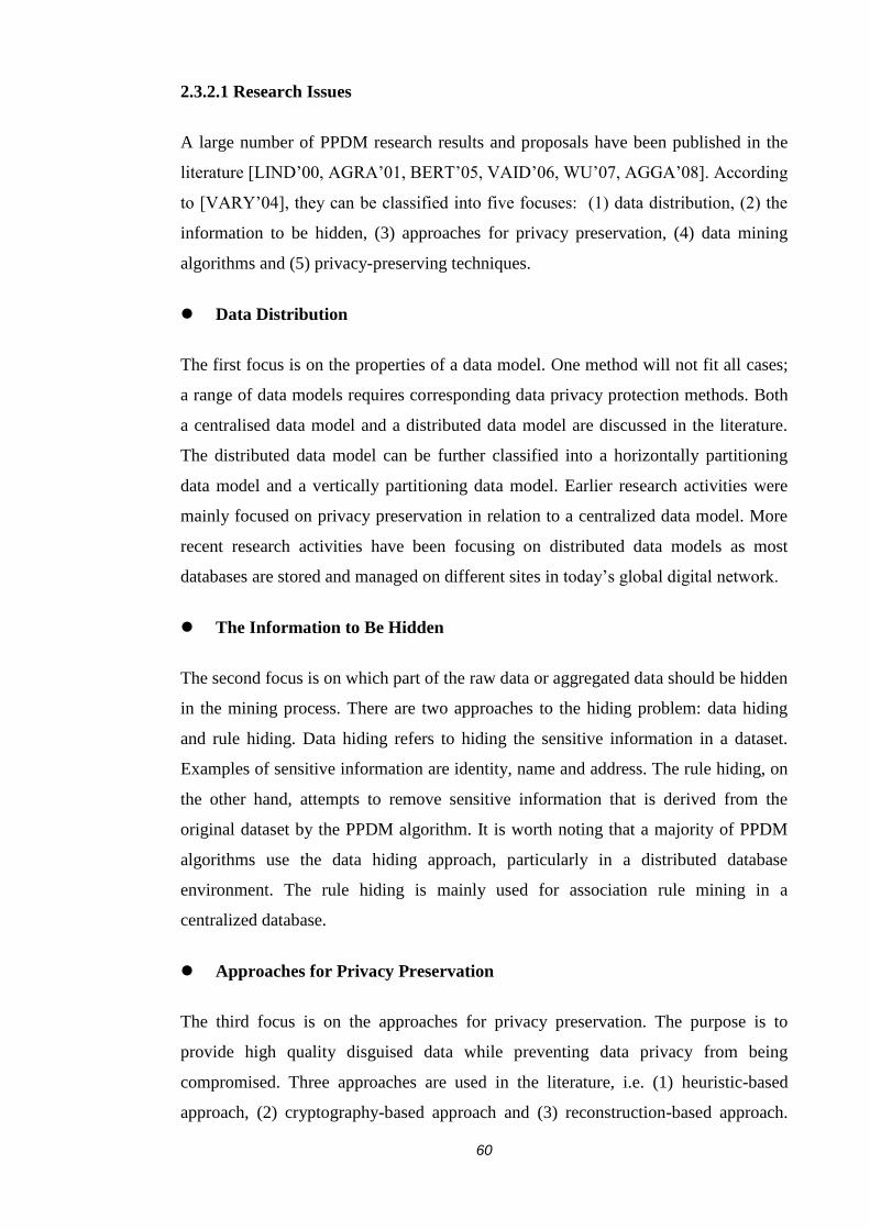
60

2.3.2.1 Research Issues

A large number of PPDM research results and proposals have been published in the

literature [LIND’00, AGRA’01, BERT’05, VAID’06, WU’07, AGGA’08]. According

to [VARY’04], they can be classified into five focuses: (1) data distribution, (2) the

information to be hidden, (3) approaches for privacy preservation, (4) data mining

algorithms and (5) privacy-preserving techniques.

Data Distribution

The first focus is on the properties of a data model. One method will not fit all cases;

a range of data models requires corresponding data privacy protection methods. Both

a centralised data model and a distributed data model are discussed in the literature.

The distributed data model can be further classified into a horizontally partitioning

data model and a vertically partitioning data model. Earlier research activities were

mainly focused on privacy preservation in relation to a centralized data model. More

recent research activities have been focusing on distributed data models as most

databases are stored and managed on different sites in today’s global digital network.

The Information to Be Hidden

The second focus is on which part of the raw data or aggregated data should be hidden

in the mining process. There are two approaches to the hiding problem: data hiding

and rule hiding. Data hiding refers to hiding the sensitive information in a dataset.

Examples of sensitive information are identity, name and address. The rule hiding, on

the other hand, attempts to remove sensitive information that is derived from the

original dataset by the PPDM algorithm. It is worth noting that a majority of PPDM

algorithms use the data hiding approach, particularly in a distributed database

environment. The rule hiding is mainly used for association rule mining in a

centralized database.

Approaches for Privacy Preservation

The third focus is on the approaches for privacy preservation. The purpose is to

provide high quality disguised data while preventing data privacy from being

compromised. Three approaches are used in the literature, i.e. (1) heuristic-based

approach, (2) cryptography-based approach and (3) reconstruction-based approach.

61

The heuristic-based approach modifies only the selected values in the original dataset,

which helps to minimize the utility loss of a disguised dataset. This approach is

mainly used for centralised databases. The cryptography-based approach preserves

privacy by means of encryption schemes and is mainly used for distributed databases.

The reconstruction-based approach reconstructs the distribution of the original dataset

using randomised dataset. With this approach, the sensitive raw data are hidden by

employing perturbation techniques based on probability distributions.

Data Mining Algorithms

The fourth focus is on the design of data mining algorithms. Most existing PPDM

algorithms are designed for performing data classification, association rules mining

and data clustering. Data classification is the process to find a set of properties that

describe and distinguish data classes. These properties can be used to classify or

predict the class of an unclassified data object. Association rule mining is a process to

discover the patterns and rules in a dataset. Data clustering concerns the problem of

decomposing or partitioning a dataset into some data groups so that the features of a

data input in a group is more similar to other data records in the same data group.

Privacy-preserving Techniques

The fifth focus is on the types of privacy-preserving techniques (also known as data

disguising techniques in some literature) that should be used in designing a PPDM

algorithm. A privacy-preserving technique is used to modify an original dataset before

its release to the computation, in order to protect data privacy. It is essential that the

privacy-preserving techniques should be in line with privacy requirements adopted by

the data providers. Privacy-preserving techniques can be largely divided into two

categories: data perturbation techniques and cryptographic primitives. Data

perturbation techniques include data alteration, data blocking, data aggregation, data

suppression data swapping and data sampling. Cryptographic primitives involve all

cryptographic schemes.

2.3.2.2 Review of PPDM Solutions

A number of privacy-preserving solutions have been developed to address a

corresponding number of data mining problems, for example, clustering, association

rule mining and classification problems. This section reviews these PPDM solutions

62

based on the three major approaches, namely, the heuristic-based, the reconstruction-

based and the cryptography-based approaches.

Heuristic-based Approach

Oliveria et al. have proposed the heuristic-based approach to address the privacy-

preserving frequent item sets mining problem in [OLIV’02]. The focus of this work is

to hide the set of frequent patterns which contain highly sensitive information. A set

of sanitized algorithms are proposed in this paper, which are used to remove certain

pieces of information from a transactional database. An item-restriction method is

used in designing these algorithms. By doing so, the addition of noise data to real data

can be avoided and the removal of real data can be limited. Three quantitative metrics

are introduced to evaluate the proposed algorithms. These three metrics are (1) Hiding

Failure, (2) Misses Cost and (3) Artifactual Pattern. The hiding failure is measured as

the percentage of restrictive patterns that are discovered in the sanitized database. The

misses cost is measured as the percentage of non-restrictive patterns that are hidden

after the sanitization process. The artifactual pattern is measured as the percentage of

discovered patterns that are artefacts. The efficiency of the algorithms is measured in

terms of CPU time. More specifically, three different methods are proposed to

measure the dissimilarity between the original and sanitized database. The first

method is based on the difference between the frequency histograms of the original

and the sanitized databases. The second method is based on computing the difference

between the sizes of the sanitized and the original databases, while the third method is

based on a comparison between the contents of the two databases.

A heuristic-based solution to protect the privacy of raw data through the use of

generalization and suppression techniques is proposed in [SWEE’02b]. The solution

achieves Anonymityk [SWEE’02a]. A release of a database is said to adhere

Anonymityk if each record in the release can not be distinguished from at least

1k other records in the release. It is then called a anonymousk database. By

performing generalization operations on the values of some target attributes, a

database A can be converted into a new database 'A that guarantees the

Anonymityk property for the sensitive data inputs. As a result, in a computation

process of seeking Anonymityk , such attributes are easily influenced by data

distortion owing to the different level of data generation the computation has applied.

63

The concept of “precision” is also introduced in this paper. Given a table T , the

precision represents the information loss incurred by converting the table T to a k -

anonymous table kT . The precision of the table kT is measured as one minus the sum

of all cell distortions, normalized by the total number of cells. It is worth noting that

in the case where generalization techniques are adopted by a PPDM algorithm for

hiding sensitive information, the precision can also be viewed as a measure of the data

quality or the data utility of the released table.

Reconstruction-based Approach

A reconstruction-based technique is proposed in [AGRA’00]. This technique is used

to estimate the probability distribution of original numeric data values in order to

build a decision classifier from a disguised dataset. A quantitative measure is

proposed to evaluate the level of privacy offered by a method and evaluate the

proposed method against this measure. The privacy provided by a reconstruction-

based technique is measured by evaluating how closely the original value of a

modified attribute can be determined. More specifically, the interval that a value x

lies within with c % confidence can be measured and the width of this interval can be

viewed as the level of privacy with a c % confidence interval. The accuracy of the

proposed algorithms is also assessed for Uniform and Gaussian perturbation under a

fixed privacy level. The approach proposed in [AGRA’01] is based on an expectation

maximization (EM) algorithm for distribution reconstruction. The reconstructed

distribution converges to the EM estimate of the origination distribution on the

perturbed data. The metrics proposed in this paper provide a quantification and

measurement of privacy and information loss. The average conditional privacy of an

attribute A , modelled with a random variable B , is defined as )|(2 BAh , where )|( BAh

is the conditional differential entropy of A given B . This information loss measures

the lack of precision in estimating the original distribution from the perturbed data.

The information loss is defined as half the expected value of the 1L -norm between the

original distribution and the reconstructed distribution. Both proposed metrics are

universal so that they can be used in measuring any reconstruction algorithm. This

application is independent of the type of data mining task applied.

A framework for mining association rules from transactions consisting of categorical

items is proposed in [EVFI’02]. This framework ensures that only true association

64

rules are mined when mining on randomized data. A formal definition of privacy

breach and a class of randomization operators are provided in this paper, which offers

a more efficient way of limiting privacy breaches than the uniform randomization.

The privacy breach is represented as the counts of the occurrences of an itemset in a

randomization transaction and in its sub-items in the corresponding non randomized

transactions. The item causing the worst privacy breach is then chosen from all sub-

items of an itemset. The worst and the average of this breach level are computed over

all frequent itemsets for each combination of transaction size and item size. The item

size giving the worst value for each of these two values can therefore be selected.

Cryptography-based Approach

A cryptography-based technique is proposed in [KANT’02]. This technique deals

with the problem of secure mining of association rules over horizontally partitioned

data. Cryptographic techniques are employed in this technique to minimize the

information shared. This approach assumes that each party first encrypts its own

itemsets using commutative encryption, then itemsets from all the other parties. An

initiating party then transmits its frequency count, plus a random value, to its

neighbour. After receiving this message from the initiating party, the neighbouring

party also adds its frequency count to this message, which it then passes on to the

other parties. Finally, the initiating party and the final party collaboratively perform a

secure comparison to determine whether the final result is bigger than the threshold

plus the random value. The proposed methods are evaluated in terms of

communication and computation costs. The communication cost is measured using

the number of message exchanges among the parties. The computation cost is

measured using the number of encryption and decryption operations required by the

algorithm. Another cryptography-based approach is presented in [VAID’02], which

addresses the problem of association rule mining in vertically partitioned data. In

particular, it aims at determining the item frequency when transactions are distributed

across different sites, while preserving the contents of each transaction. A security and

communication analysis is also performed in this paper. The security feature of this

protocol for computing the scalar protocol is analyzed. The total communication cost

of this solution depends on the number of candidate itemsets.

65

2.3.2.3 Summary of PPDM Research Results

Figure 11 summarizes the existing efforts and approaches in the field of PPDM

algorithm designs based on the aforementioned discussions.

Figure 11. A taxonomy of the developed PPDM algorithms. (Source: Author’s own)

2.3.3 Privacy-preserving Distributed Statistical Computation

(PPDSC)

A PPDSC technique is aimed at supporting a joint statistical computation by multiple

parties without compromising the privacy of individual datasets managed by

respective parties. Existing PPDSC solutions can be largely divided into three

categories, the statistical disclosure control (SDC), secure matrix product computation

(SMPC) and secure linear regression computation (SLRC). In general, the SDC

technique preserves data privacy by pre-processing the dataset before releasing it. The

SMPC technique serves as a building block for large dataset computation by

preserving data privacy through the use of matrix product techniques. The SLRC

technique transforms normal regression computation algorithms to privacy-preserving

66

ones in different research contexts. The details of these three techniques are given

below.

2.3.3.1 Statistical Disclosure Control

SDC is concerned with how to prevent the identification of an individual in a dataset

and the disclosure of confidential information about the dataset through the use of

statistical techniques [Will’96, WILL’01]. A formal definition of statistical disclosure

can be found in [ELLI’05]: “The revealing of information about a population unit

through the statistical match of information already known to the revealing agent (or

data intruder) with other anonymised information (or target data set) to which the

intruder has access, either legitimately or otherwise.” As a released dataset can always

be collected and stored by the data collector and then be analysed to retrieve other

information from the dataset, the disclosure of confidential information about the

released dataset is a potential problem after data dissemination. The purpose of SDC

techniques is to reduce the risk of information disclosure in disseminated datasets.

The SDC methods focus on restricting the amount of or modifying the dataset before

it is disseminated. They can be applied to two types of data: microdata and tabular

data. Microdata consists of a series of records, each containing information on an

individual unit such as a person, a company or an organisation. The simplest form of a

microdata can be represented as a single data matrix, where the rows correspond to

data subjects and the columns to the variables. Microdata is the basis for tabular data.

Tabular data is the aggregated information on data subjects presented in tables.

Frequency and magnitude data are examples of tabular data. Tabular data are

normally directly processed for statistical confidentiality. According to our literature

survey, five techniques are used to assist the disclosure control [WILL’96, WILL’01,

SHLO’07, FAYY’10, ELLI’05]: recording, cell suppression, rounding,

masking/blurring and data swapping.

Recoding is a tool that is commonly used in disclosure control solutions [HURK’98,

ELLI’05, CAST’10]. The idea of recoding is to take the raw data and re-categorise a

variable. By using this technique the variable’s attributes with lower frequencies can

be merged. A typical example is age; a single age attribute can be recoded to the age

group of 5 or 10 years. Table 3 illustrates the result of attribute recoding of Table 2. It

is also common to use this technique for income or occupation data, for example,

67

specification occupations or higher income bands can be grouped together. A special

case of recoding is top-recoding; in this case, frequencies toward the top of the

variable range are likely to be less. Table 4 illustrates the result of top-recoding of

Table 2. A common application of this technique is global recoding which involves

applying all recode universally across a file. On the other hand, localized recoding is

preferable when a variable is highly correlated with location. The advantage of

recoding is that the impact on data quality is visible. However, it changes the table

structure; as the loss of information affects the entire dataset, the benefit may be

relatively small regarding risk reduction.

Table 2. An example table of frequency count for data subjects whose age is between 1 to 10 and who live in area A1 to A4. (Source: Author’s own)

Table 3. An example of attribute recoding. (Source: Author’s own)

68

Table 4. An example of top-recoding. (Source: Author’s own)

Cell suppression, a technique used to control disclosure in a tabular or aggregated data

[SALA’06, LI’08b, CAST’10], simply means leaving this cell blank. The use of this

operation is more effective when a cell is classified as sensitive. Normally this

happens when a cell has a low or zero count and is more likely to cause cell value

disclosure. A weakness of cell suppression is that it is insufficient to suppress only the

sensitive cells, other suppressions on non sensitive cells are also needed. For example,

if only cells with small range of values are suppressed, these suppressed cells would

be identified as having a small range of values. Therefore, it would also be necessary

to suppress some other non-sensitive cells to disguise any patterns in the values of

sensitive cells and the resulting table may have less analytical data items. Given that

Table 5 is the original data which has sensitive data item in cell ),( BC , Table 6

illustrates the cell suppression result of Table 5.

Table 5. A table with sensitive cell (C,B). (Source: Author’s own)

69

Table 6. A table with sensitive cells suppressed and further complementary suppression made. (Source: Author’s own)

Rounding is a technique used to disguise the exact frequency count of a cell by

rounding every cell in a table to a given number base [SALA’06, LI’08b, CAST’10].

The base is typically set to 3, 5 or 10. In other words, rounding simply means that the

value of the data item in a cell (i.e. cell value) is rounded to one of the two closest

integer multiples of the rounding base. This technique is normally applied to

aggregate data. Table 7 illustrates the result of Table 5 where the cell values have

been randomly rounded to base 5. In this table, cell counts are rounded either up or

down randomly. One problem with this technique is that, under certain circumstances,

cell counts can not add up to the subtotals and total of the table, which makes

rounding very difficult. A more relaxed form of rounding is to round the cell values in

such a way that the cell values of the rounded table are not too far removed from the

original values. Even when the additivity is allowed, the controlled rounding can still

cause certain problems. For example, if multiple separate overlapping tables are

rounding separately, the common marginal cells would be rounded to different values;

this further reduces accuracy of the rounded table.

Table 7. A table with cell values been randomly rounded to a base of 5. (Source: Author’s own)

70

Masking /blurring techniques preserves data privacy by adding noise to the data to be

protected [ELLI’05, SHLO’07, FAYY’10]. For tabular data, this can be achieved by

adding/subtracting random integers to/from cell values. For microdata, this can be

done by simply changing the data value to other values. One advantage of these

techniques is that even if a large amount of data on a specific individual is gathered by

an intruder, the precise information of the individual is still preserved by the noise

signals. In general, the larger the variances of the noises are, the better the provision

of the disclosure protection.

Data swapping applies a sequence of elementary swaps to a dataset [DOMI’01,

ELLI’05, SHLO’07]. This execution of data swapping consists of two tasks. The first

task is to randomly select two data records in the dataset; for tabular data, this task

may be performed by randomly selecting two rows or columns in the table. The

second task is to perform the swapping of the selected data records; for tabular data,

this task is performed by swapping the selected rows or columns. This technique

performs swapping of records in a dataset/table. More specifically, if this swapping is

performed on some potential key variables or sensitive information, a better data

protection can be provided than on normal data records. For example, the swapping of

key variables and sensitive data records would harden the intruder’s data matching

task and make the matching result inaccurate. It is usually preferable to swap records

that share the same value with other variables, as this leads to less data distortion and

reduces the risk of inconsistent value combination.

2.3.3.2 Secure Matrix Product Computation

In a cooperative computational environment, the data provided by multiple data

holders may be horizontally partitioned, vertically partitioned or hybrid data. Owing

to the difficulty in expressing these data types clearly and concisely, and the fact they

often need multi-dimensional expressions, computations involving the use of any of

the above three data types are much more complex than computing equations using

one-dimensional values. Secure matrix product protocols [DU’01b, KARR’09a]

integrate cryptographic primitives (e.g. oblivious transfer protocol and homomorphic

encryption method) with linear algebra theories to compute such types of data and to

compute their mean values with privacy preservation. There are two major types of

secure matrix product protocols: the secure scalar product protocol and the secure

shared scalar product protocol. A secure scalar product protocol allows two parties,

71

Alice with her private input }...,,{ 1 nxxX , and Bob with his private input

}...,,{ 1 nyyY , to jointly compute the scalar product

n

i ii yxYX1

, securely

without revealing X and Y to the other party. In other words, after the protocol

execution, Alice learns no more information other than x and YX , and Bob learns

no more information other than y and YX . A secure shared scalar product protocol

allows two parties, Alice and Bob, to compute equation YXss BA with privacy

preservation. After the protocol execution, Alice receives As and Bob receives Bs ,

such that YXss BA . Both of the above approaches have found important

applications in developing secure solutions to distributed multiparty computation.

A number of secure scalar product protocols and secure shared scalar protocols have

been proposed in the literature [LUO’05, DU’01a, DU’04, LUO’03, KARR’09a,

DU’02, DU’01e, GOET’04, SHEN’07, WANG’09]. Du et al. proposed an invertible

matrix and a commodity-based approach [DU’04]. The former enables the trade-off

between efficiency and privacy while the latter, based on Beaver’s commodity model

[BEAV’97], achieves some performance gain by sacrificing a certain degree of

security. The secure two-party scalar-product protocol proposed by Goethals et al.

[GOET’04] relies on the intractability of the composite residuosity class problem to

achieve security. Luo et al. [LUO’03, LUO’04, LUO’05] extended Du’s secure two-

party scalar product protocol to three-party scenarios and developed a set of real

product protocols: a real product protocol, two add-product protocols, a division

protocol, a exponential function protocol, a power function protocol , a logarithmic

function protocol and a trigonometric function protocol. These protocols can be used

to resolve several specific problems, such as secure exponential function computation

problem, secure power function computation problem and secure logarithmic function

computation problem. All of these protocols are designed based on the secure scalar

product protocol, which sheds some light on finding secure solutions to support

distributed multiparty computation.

2.3.3.3 Secure Linear Regression Analysis

Regression analysis is often used to identify patterns, and/or make predictions based

on available datasets. For example, a French diabetic research institute and a British

diabetic centre would like to find if there is any correlation between specific medical

conditions and factors such as education, sex, age, income and career between the two

72

sets of patients under their respective managements using regression analysis method.

In addition, they would also like to identify future trends in some of these factors in

order to take preventive measures against diabetes and other related diseases. Owing

to the privacy concerns and legal responsibility, they can not reveal their patients’

records to the other party. In this case, privacy-preserving regression methods can be

used to find hidden trends and other valuable information related to this problem.

The design of a privacy-preserving regression protocol largely makes use of secure

matrix operation protocol and secure scalar product protocol. To date, a number of

such protocols have been proposed [DU’01b, DU’01d, LUO’03, DU’04, KARR’04,

REIT’04, KARR’05a, KARR’05b, KARR’06, KARR’09a]. The most notable ones

are the secure simple linear regression protocols [LUO’03, DU’01b, DU’01d,

KARR’06], secure multivariate regression protocol [DU’04] and secure regression

protocols for vertically partitioned and partially overlapped data [KARR’04, REIT’04,

KARR’09a]. Among these works, the secure simple linear regression protocol

designed by Du et al. [DU’01d] uses the secure scalar product protocol to address the

linear regression inference in a two-party homogeneous data model. The secure

multivariate linear regression protocol proposed in [DU’04] uses the matrix product

protocol and the commodity–server solution. Built on the secure matrix protocol,

these solutions can securely compute matrix inverse, matrix determinant and norm.

Furthermore, the paper [DU’04] allows two parties to evaluate more complicated

mathematical expressions than merely computing the matrix product or dot product

operations. Karr et al. [KARR’05a] proposed a framework to address the secure linear

regression problem in a cooperative environment in which protecting the sources of

data records is the primary concern. The framework was developed by using local

computation and secure summation protocol. With this framework, the computational

process is as follows. First, it uses the additivity property of the linear regression

model to compute the regression coefficient. At the second step, the framework

supports the use of two approaches. The first approach applies local computation and

secure summation to compute and exploit additivity of several statistics to diagnose

the corresponding statistical model (secure data integration model and securely shared

local statistics model) [KARR’05a]. The second approach generates synthetic

residuals to perform model diagnostics while preserving the relationships among

predictors and residuals. More specifically, the solutions to secure two-party

computation of simple regression analysis were designed by employing scalar product

73

techniques [DU’01a, DU’01b, DU’01c, LUO’03, KARR’05b]. In [DU’01a, DU’01b],

the computation of variance and correlation coefficient were discussed regarding both

heterogeneous data model and homogeneous data model. The Secure Two-party

Statistical Analysis Protocol in Heterogeneous Model securely computes the

correlation coefficient r and the slope of the simple linear regression line b , where

Alice has a dataset )...,,( 11 nxxD and Bob has a dataset )...,,( 12 nyyD , while

Division Protocol and the Secure Two-party Statistical Analysis Protocol in

Homogeneous Model compute r and b , where Alice has dataset

)),(...,),,(( 111 kk yxyxD and Bob has dataset )),(...,),,(( 112 nnkk yxyxD . Luo

[LUO’03] further extended Du’s protocol [DU’01d, DU’04] to address the secure k-

party regression problem in a homogeneous model using secure real product and

division protocols. A solution was designed to securely compute

x ,

y , r and b ,

where party1 has )),(...,),,((11111 ss yxyxD , party2 has

)),(...,),,((2211 112 ssss yxyxD , …, partyk has )),(...,),,(( 11 11 kkkk ssssk yxyxD

. A

similar solution was found in [KARR’05b] to perform secure statistical analysis on

distributed chemical databases, which has demonstrated a real life application of this

solution.

Solutions to multivariate linear regression analysis were studied and presented in

[DU’04, REIT’04, KARR’06]. In [DU’04], the authors consider the joint dataset

M as a )1)(( mnN matrix, where

NmnNNN

mnn

nNN

n

y

y

xx

xx

xx

xx

M

1

,1,

,11,1

,1,

,11,1

.

Each column of M is represented as an attribute, so there are 1mn attributes in

M . Each row of M represents a data subject’s values of these attributes. It is further

defined that

mnNNN

mnn

nNN

n

xx

xx

xx

xx

X

,1,

,11,1

,1,

,11,1

and

Ny

y

Y 1

. To find the

regression coefficient of XY that best fits M is the purpose of this

computation. [DU’04] considers a two-party, vertically partitioned data model, where

Alice has

nNN

n

xx

xx

A

,1,

,11,1

, and Bob has

mnNNN

mnn

xx

xx

B

,1,

,11,1

. Several

74

protocols were proposed to support intermediate computational tasks in a multivariate

regression computation while preserving the privacy for A and B . The techniques of

matrix product computation, inverse matrix computation and random noise generation

were used for hiding A and B . The intermediate computation results were also

disguised by random noise, so that they can not be used to infer useful information.

The authors also demonstrate that this secure multivariate regression solution can be

applied to build multivariate classification model without disclosing the raw data.

An interesting extension of the secure multivariate regression computation can be

found in [REIT’04]. This paper considers a special data partitioning model: the

vertically partitioned, partially overlapping data, where multiple parties hold datasets

for different variables; some of the variables, however, are overlapped. These parties

would like to find the regression function that best fits their joint dataset, but none of

them is willing to share their raw data with other parties. This paper addresses

problems for datasets that are multivariate normal and multinomial distributions. The

expectation maximization algorithm was used as a building block in this paper. The

parties only compute and share the sufficient statistics required for the building block,

rather than sharing individual data values of their respective dataset. A framework for

secure linear regression and statistical analyses in a cooperative environment was

proposed in [KARR’06]. It summarized the research results regarding secure linear

regression related computation problems under various forms of data partitioning

models.

2.4 Identification of the Research Gap

From the above literature reviews and related work analyses, we have observed that,

despite the increasing number of emerging needs for secure computation of a number

of statistical algorithms, only a subset of these algorithms have actually been

converted into privacy-preserving solutions, i.e. the statistical disclosure, the matrix

product computation and the linear regression analysis. Most of the privacy-

preserving statistical computation problems are yet to be explored. Hypothesis tests,

factor analyses and nonlinear regressions are examples of the statistical algorithms

that find applications in privacy-preserving collaborative computation environments,

but have yet to be transformed into privacy-preserving protocols. To address this gap,

this thesis, as our initial effort, investigates security methods in search of an optimum

75

solution to privacy-preserving distributed statistical computation problems. The

nonparametric sign test (NST) is chosen as a case for study. Through the

demonstration of how to convert a nonparametric hypothesis test (NST) algorithm

into a privacy-preserving protocol that could support privacy-preserving distributed

statistical computation in a cost-efficient manner, a four-phase methodology has been

developed. This methodology can be used to transform any other statistical

computation into privacy-preserving ones.

Most importantly, to transform a conventional computational algorithm into a secure

and cost-efficient protocol, the algorithm will first be examined and divided into local

and global computation tasks. The results from a local computational task or a global

computation task are so-called intermediate computational results that will need

privacy protection. A global computational task can lead to the identification of

interactions among multiple parties. The messages used in these interactions can be

intermediate computational results and/or original input from the sender. The original

input may contain raw data of the original dataset and the intermediate computational

results may contain aggregated information of the joint dataset.

How to protect the privacy of these original input data, intermediate computational

results and/or interaction messages is a challenging task which is dependent on the

nature and characteristics of the computation algorithms. In addition, there are a wide

range of privacy-preserving building blocks that can be used to preserve data privacy.

These building blocks may have different security capabilities and impose

corresponding storage and computational requirements. Which set of building blocks

should be chosen and how to apply them to best achieve privacy-preserving

collaborative computation in a cost efficient manner is the focus of this research. For

proof of this concept, the NST algorithm is chosen as the case for study. The ultimate

goal of this research is to find an optimum solution to the PPDSC problems.

2.5 The Best Way Forward

A systematic approach has been employed in the design of our solutions to privacy-

preserving nonparametric sign test (P2NST) computation. This approach can be

divided into the following steps:

76

To investigate research gaps in the literature.

To investigate data privacy definitions in the literature. Thus the properties of

sensitive information and why this information needs to be protected can be

understood.

To define data privacy in the P2NST computation.

To investigate privacy-preserving primitives in literature. The properties and

capabilities of privacy-preserving primitives in the literature can then be learnt.

To apply the most appropriate privacy-preserving primitives in the design of

our P2NST solution in search of an optimum cost-efficient solution.

To implement and evaluate the designed solution.

To conclude the lesson learnt from this research.

2.6 Chapter Summary

This chapter has presented an intensive overview of the-state-of-the-art methods in

the privacy-preserving distributed computation. The terminologies and definitions that

are used in the field of PPDDC were first introduced and defined. Following an

investigation into the privacy concerns in both legal and research areas, the privacy-

preserving solutions that were proposed in the related works in the literature were

studied. This began with SMC solutions, which is the origin of this research topic,

followed by studying solutions in the area of PPDM, which is a new research area that

applies the secure multiparty computation techniques to knowledge discovery.

Finally, the PPDSC solutions were studied. From these reviews, the gap in current

research has been identified. This chapter then outlined our ideas in designing

solutions to the P2DNST computation. Before describing the design of our proposed

solutions to the problem identified, the next chapter provides the design preliminaries

and evaluation method of this research work while chapter 4 presents the privacy-

preserving building blocks to be used in the design of our solutions.

77

Chapter 3 Design Preliminaries and Evaluation Method


This chapter outlines the design preliminaries and evaluation method of the solutions

presented in this thesis. In detail, the data privacy definitions used in the design of our

solutions are described in section 3.2. Section 3.3 provides the decomposition and

analysis of the original nonparametric sign test (NST) algorithm. Section 3.4 specifies

the design requirements for the privacy-preserving solutions. The evaluation strategy

of the designed solutions is drawn up in section 3.5 while section 3.6 details the

simulation method. Finally, section 3.7 summarizes this chapter.

3.2 Definition of Data Privacy

Based on the privacy definitions in [CLIF’02b, GOLD’04], this thesis makes use of a

three layer privacy definitions: individual data confidentiality, individual privacy and

corporate privacy.

Definition 3.1: Individual Data Confidentiality

Individual data confidentiality refers to preserving the secrecy of an individual data

item so as to ensure that the data item is only accessible to the data provider that

manages the data item.

Definition 3.2: Individual Privacy

Individual privacy refers to the privacy of a data subject. Let us assume that data

items are collected from a data owner (i.e. a subject) by two or more data (or service)

providers (e.g. Alice and Bob). Preserving individual privacy means that, upon a

successful computation of function, f , among multiple data providers (e.g. Alice and

Bob), information in relation to the subject should not be disclosed to parties other

than the managing party of the subject, i.e. Alice or Bob.

The meaning of keeping a data item in private is twofold. Firstly, it means preserving

the confidentiality of the data item. Secondly, the data subject to whom the data object

is associated should not be identifiable from the data item. In other words, during a

78

computational process, the data item should be protected from access by any party

other than the managing party itself. In the event of a protected data item being

revealed, it can not be used to identify the owner/data subject of the data item. More

formally, assuming that },...,,{ ,2,1, kiiii ssss , where is represents subject i ’s data

itemset consisting of k different items (or objects) and jis , is subject i ’s thj data

item, where kj ,...,2,1 . To preserve the data privacy, the real value of jis , should

be prevented from being revealed (i.e. this preserves the data confidentiality of a data

item), and furthermore, even if the confidentiality of jis , is compromised, this will not

be sufficient for a perpetrator to understand that the owner of this data is subject i (i.e.

this preserves the individual privacy in relation to a data item).

Definition 3.3: Corporate Privacy

Corporate privacy refers to the privacy of data providers’ local statistics, which

contain various levels of aggregated information of the dataset. That is, upon the

computation of a function, f , information in relation to a participating party’s local

statistics, for example, the mean value or the median of },...,,{ ,2,1, kiii sss , should not be

revealed to any other party than the contributor itself.

Quantification of Data Privacy

As the solutions designed in this thesis are developed based on data perturbation

techniques, such as data randomization, data swapping and data transformation

techniques, we use the metric proposed in [AGRA’01] to quantify the security level of

our solutions. This metric is designed based on the work of [AGRA’00] and

Shannon’s information entropy theory [SHAN’48].

Shannon defines the concept of entropy as follows: Let X be a random variable

which takes on a finite set of values according to a probability mass function )(xp .

Then, the entropy of the random variable X is defined as follows: In discrete cases,

))((log)()( 2 xpxpXh . In continuous cases, dxxfxfXh ))((log)()( 2 ,

where )(xf denotes the probability density function (pdf) of the continuous random

variable x . It has been widely used in the literature that )(Xh is a measure of

uncertainty in the value of X [AGRA’01]. For example, for a random variable U

79

uniformly distributed between 0 and a , the entropy is )(log)( 2 aUh . Entropy

represents the information content of a datum, the entropy after data sanitization

should be higher than the entropy before the sanitization.

The authors of [AGRA’01] use the property of measure of uncertainty of entropy to

measure the level of privacy. It defines that given a random variable A with

probability density function )(afA , the differential entropy )(Ah of A is described

as follows: daafafAh AAA))((log)()( 2 , where

A is the domain of A . The

authors further propose a measure of privacy of the random variable A as

)(2)( AhA i.e. aAaAh

)(log)( 222)( . Here )(A denotes the length of an

interval over which a uniformly distributed random variable has the same uncertainty

as A . This quantifies the level of privacy by means of its uncertainty.

3.3 The NST Computation

In this section, the NST computation is used as an exemplar algorithm to demonstrate

how to transform a statistical algorithm into a distributed privacy-preserving one such

that multiple mutually distrustful parties can compute the algorithm on their joint

dataset without compromising their respective privacy.

The NST algorithm will firstly be described and then transformed into one that can be

executed in an ideal Trusted Third Party (TTP) based model (here after called the

TTP-NST algorithm). Through this transformation process, it is possible to identify

the computational elements (or segments) that could be performed by an individual

party itself without any input from, or the involvement, of other parties (i.e. the so

called local computation), and from the elements that require inputs from, or the

participation of, other parties (i.e. the so called global computation). In addition, all

intermediate results (i.e. those are generated from earlier stages of a computation and

will be used to compute the next intermediate result or the final result) will also be

identified and singled out from the final result (that is the final outcome of the

computation).

Based upon the nature of these local/global computation tasks and intermediate/final

computational results, we can then investigate, identify or design the most appropriate

privacy-preserving techniques or protocols and use them to support the NST

80

computation without the involvement of the TTP. This can be achieved while

simultaneously preserving the privacy of participating parties’ respective inputs and

intermediate computational results. In other words, our main task is to seek and

design privacy-preserving primitives and protocols and use them to replace the

involvement of the TTP so as to transform the TTP-NST algorithm into a privacy-

preserving distributed NST algorithm (here we call it P2DNST). By using the

P2DNST algorithm, the parties should learn no more than if they were using the TTP-

NST model.

Two data partitioning models are considered in the protocol design, i.e. the vertically

partitioned (heterogeneous) data model and the horizontally partitioned

(homogeneous) data model. In the vertically partitioned data model, Alice has

}...,,{ 1 nxxX and Bob has }...,,{ 1 nyyY . The sign test computation using this data

partitioning model involves pairwised comparison for each ),( ii yx . Alice and Bob

will need to send their respective private datasets into the computation in order to

compute the sign test result. During the course of the sign test computation,

}...,,{ 1 nxxX and }...,,{ 1 nyyY are first compared pairwised. A set of

intermediate results is then generated, i.e. ),,( RQP , where P is the number count of

ii yx , Q is the number count of ii yx and R is the number count of ii yx .

),,( RQP is then used to compute the sign test result.

On the other hand, in a horizontally partitioned data model, Alice holds a dataset

)},(...,),,{(1111 nn yxyxA of 1n data subjects and Bob holds a dataset

)},(...,),,{(2211 nn yxyxB of 2n data subjects. For computing sign test, Alice can

calculate AP , AQ and AR from A , where AP is the number count of ii yx ; AQ is

the number count of ii yx ; AR is the number count of ii yx , where 1,...,1 ni .

Likewise, Bob can compute BP , BQ and BR from B , where BP is the number count

of ii yx ; BQ is the number count of ii yx ; BR is the number count of ii yx ,

where 2,...,1 ni . In this data model, Alice and Bob only need to send ),,( AAA RQP

and ),,( BBB RQP , respectively, to the computation in order to perform the

collaborative sign test computation. This computation is simpler than that of a

vertically partitioned data model as it only needs intermediate results from Alice and

Bob, respectively. These intermediate results do not contain any private information

81

regarding individual data confidentiality and individual privacy. Its solution can be

easily deduced from the solution of the vertically partitioned data model solution.

This thesis focuses on the design of solutions to vertically partitioned data model. The

horizontally partitioned model case will be left as our future work.

3.3.1 The NST Computation Problem

Assuming that Alice has a dataset }...,,,{ 21 nxxxX and Bob has a dataset

}...,,,{ 21 nyyyY , and X and Y are dependent and paired datasets, where ix and iy

are both generated from subject i , for ni ...,,1 . To start with, we also assume each

object only generates a single data pair and contributes to Alice and Bob respectively.

In this case, X and Y are vertically partitioned (or homogeneous) datasets. Both

Alice and Bob want to know if there is any difference between }...,,,{ 21 nxxxX and

}...,,,{ 21 nyyyY by performing NST, under the -significance level. Formally,

this is a hypothesis test problem with respect to a null hypothesis 0H , for example,

0H : The two population distributions are identical and 5.0)Pr( ii yx for any pair;

versus an alternative hypothesis 1H , for example, 1H : The two population

distributions are not identical and 5.0)Pr( ii yx for any pair, under the -

significance level.

3.3.2 The TTP-NST Algorithm

As neither Alice nor Bob is willing to reveal any value of their respective datasets to

the other party during the computation, they would like to perform this computation

with privacy protection. One way of achieving this is through the use of a TTP. In this

TTP based model, Alice and Bob send their respective datasets to the TTP, and the

TTP uses the data to perform the computation, and then sends the outcome of the

computation to Alice and Bob, respectively. As the TTP is the centre of the

computation, the level of privacy protection afforded in this model lies in the

trustworthiness of the TTP. If the TTP is fully trustworthy, and if it only delivers the

final result to the parties, it is clear that nobody could learn anything that is not

inferable from its own input and the final result, assuming that such a TTP does exist.

The operation of this computation is shown in Figure 12 and the computation process

is expressed in pseudo code in Figure 13.

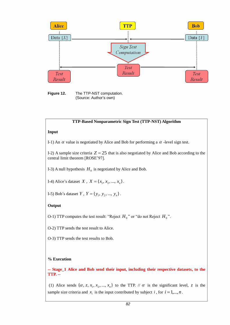
82

Figure 12. The TTP-NST computation. (Source: Author’s own)

TTP-Based Nonparametric Sign Test (TTP-NST) Algorithm

Input

I-1) An value is negotiated by Alice and Bob for performing a -level sign test.

I-2) A sample size criteria 25Z that is also negotiated by Alice and Bob according to the

central limit theorem [ROSE’97].

I-3) A null hypothesis 0H is negotiated by Alice and Bob.

I-4) Alice’s dataset X , }...,,,{ 21 nxxxX .

I-5) Bob’s dataset Y , }...,,,{ 21 nyyyY .

Output

O-1) TTP computes the test result: “Reject 0H ” or “do not Reject 0H ”.

O-2) TTP sends the test result to Alice.

O-3) TTP sends the test results to Bob.

% Execution

-- Stage_1 Alice and Bob send their input, including their respective datasets, to the

TTP. --

(1) Alice sends }...,,,,,{ 21 nxxxz to the TTP. // is the significant level, z is the

sample size criteria and ix is the input contributed by subject i , for ni ,...,1 .

83

(2) Bob sends }...,,,,,{ 21 nyyyz to the TTP. // is the significant level, z is the

sample size criteria and iy is the input contributed by subject i , for ni ,...,1 .

-- Stage_2 TTP calculates intermediate results P, Q, R and N. --

(3) For 1i to n , TTP compares ix and iy .

if ii yx , then TTP generates }0,0,1{},,{ iii RQP ;

else ii yx , then TTP generates }0,1,0{},,{ iii RQP ;

else ii yx , then TTP generates }1,0,0{},,{ iii RQP ;

end if,

end.

(4) TTP calculates

n

i iPP1

. // P is the number counts of positive signs.

(5) TTP calculates

n

i iQQ1

. //Q is the number counts of equal value.

(6) TTP calculates

n

i iRR1

. // R is the number counts of negative signs.

(7) TTP calculates QnN . // N is the sum of number counts of positive signs and

negative signs.

-- Stage_3 TTP calculates intermediate results 0T , CR, 1T and 2T . --

(8) TTP calculates },min{0 RPT .

if RP , then let RT 0 ;

else RP , then let RPT 0 ;

else RP , let test statistic PT 0 .

(9) TTP calculates the critical value CR according to N , Z and .

if ZN , then 2

CR ;

else ZN , then find CR from Standard Normal Distribution Table according to N

and .

(10) TTP calculates the test statistic T ,

84

if ZN , then let test statistic NT

i

T

i

NT

iiTi

TCTT )

2

1(

)!(!

!)

2

1(

00 0

00

0

01 ;

else ZN , let test statistic

2

2)5.0( 0

2N

NT

TT

.

-- Stage_4 TTP performs the Sign Test computation --

(11) TTP compares T and CR ,

if CRT , then reject 0H ;

else do not reject 0H .

-- Stage_5 TTP transmits the final computational result to Alice and Bob, respectively.

--

(12) TTP sends the test result to Alice.

(13) TTP sends the test result to Bob.

(14) end of this computation.

Figure 13. The TTP-NST algorithm. (Source: Author’s own)

As shown in Figure 13, the TTP-NST algorithm can largely be divided into five

computational stages:

Stage_1) TTP gathers inputs }...,,,{ 21 nxxx and }...,,,{ 21 nyyy from Alice and Bob,

respectively.

Stage_2) TTP performs the comparison for each ),( ii yx and generates Stage_2

intermediate results P , Q , R and N .

Stage_3) TTP generates Stage_3 intermediate results 0T , CR , 1T and 2T , using the

intermediate results of Stage_2.

Stage_4) TTP performs the sign test according to the intermediate results of Stage_3

and obtains the test result (final result).

85

Stage_5) TTP sends the final result to Alice and Bob.

These fives stages enable us to specify the design requirements which can be found in

the next subsection.

3.4 Design Requirements

From the TTP-NST algorithm decomposition, it can be seen that the data privacy

protection in this computation heavily relies on the trustworthiness of the TTP, who

has access to the datasets from both Alice and Bob. If the TTP exposes any

information in relation to the dataset of a party (Alice/Bob) to the other party

(Bob/Alice), the concerned party’s data privacy would be compromised. In addition,

the TTP also knows the intermediate results of the computation, which, if disclosed,

may be used by either of the parties to infer useful information about its counterpart’s

input. The detailed analysis is given below.

In order to design a solution that does not need a TTP, the following four

requirements should be carefully addressed.

Requirement 1: To Protect the Privacy of Input Data Items

According to the assumption of sign test, Alice has }...,,,{ 21 nxxxX , Bob has

}...,,,{ 21 nyyyY and ),( ii yx comes from subject i , for ni ...,,2,1 . The first

objective of this computation is to protect }...,,,{ 21 nxxx from Bob and protect

}...,,,{ 21 nyyy from Alice during the computation. Therefore, we need privacy-

preserving techniques here, to support two-party privacy-preserving (or secure)

comparison of ),( ii yx , where ni ...,,2,1 . After the comparison, Alice only knows

ix and the comparison result; Bob only knows iy and the comparison result.

Requirement 2: To Protect the Difference Between ix and iy

After the pairwised comparison, if the value of )( ii yx is known by either Alice or

Bob, the value of iy or ix can be calculated. This breaches the individual data

confidentiality of ix or iy , and individual privacy of iS . This information can be

86

further used to infer other data items in X or Y . The more data items are inferred, the

more accurately the aggregated information can be estimated.

Requirement 3: To Protect the Privacy of Intermediate Results

As discussed above, during the process of the computation, several intermediate

results are generated, which may be used to infer information about }...,,,{ 21 nxxx

and }...,,,{ 21 nyyy . For example, in the TTP-NST algorithm, the intermediate results

are: P , the number count for ii yx ; Q , the number count for ii yx ; R , the

number count for ii yx ; N , the number count for ii yx , where RPQnN ;

CR , the critical value of this test; 0T , the intermediate result that equals to },min{ RP ;

1T , the test statistic if this is a small-size sign test, and 2T , the test statistic if this is a

large-size sign test. All these intermediate results should be protected. For example, if

Alice gets P , she may infer the value of RQ ; if P or RQ are approximating to

n , Alice might infer the distribution of the joint dataset. If Alice gets both P and Q ,

then she can not only perform the test by herself, but also derive the characteristics of

Bob’s dataset, which compromises the corporate privacy of Bob’s dataset.

Furthermore, in some extreme cases, if a significant amount of information coexists in

the joint datasets, individual privacy and corporate privacy may both be compromised.

For example, some outliers are existed in the joint dataset or the dataset provided by

Alice which is centred to a specific point. It is thus also necessary to secure these

intermediate results using cryptographic means.

By examining the TTP-NST algorithm, it can be seen that the issue of preserving the

privacy of intermediate results affects three stages of the computation: Stage_2,

Stage_3 and Stage_4. As the intermediate results from Stage 2 will be fed into the

computation performed in Stage_3, and the intermediate results from Stage_3 will be

fed into the computation at Stage_4, we need to examine how these intermediate

results can be protected while rendering the computation in the successive stage

possible. For example, four intermediate results are generated in Stage_2: P , Q , R

and N . Because Q contains equal information to N (i.e. QnN ), this

information should be used at Stage_3 to determine the sample size and to find the

CR value. In addition, the value of P and R should also be used to generate the

intermediate result 0T . We need to apply a secure random permutation function to

87

protect the values of P and R , so that even if Alice knows either of the values, she

still needs to spend concerted efforts on guessing the value of P or R , and the

probability of her correctly guessing the value of P or R is 0.5, respectively.

Requirement 4: To Identify Privacy-preserving Techniques

Privacy-preserving techniques should be selected so that the aforementioned security

issues can be appropriately addressed. Once these have been identified, the design of

the P2DNST solution can be commenced.

In addition, four other parameters are also used in the computation, they are z , , n

and CR . Where z is the sample size criterion (negotiated by Alice and Bob prior to

the computation); is the significance level (negotiated by Alice and Bob, also prior

to the computation); n is the number of data subjects; CR is the critical value for the

test and is defined by z , N and . The privacy issues in relation to these four

parameters can be discussed in terms of individual privacy and corporate privacy.

Firstly, disclosing the four parameters does not breach the individual privacy of each

subject or the data inputs. Secondly, the only corporate privacy breached by the four

parameters is the value of RP (= N ), as N is needed to find CR . However,

knowing RP can not help one party to infer information about the other party’s

dataset nor can it be used to infer aggregate information of the other party. In other

words, disclosing RP is acceptable during the execution of the algorithm, in order

to achieve a desired level of privacy preservation.

3.5 Evaluation Strategy

The performance of the designed solutions will be compared with the TTP-NST

algorithm. To do so, the designed solutions will be evaluated with respect to the

following metrics: the correctness, the security level, the computation overhead, the

communication overhead and the protocol execution time. These metrics are

explained below.

3.5.1 Correctness

To ensure that the final computation results of the two privacy-preserving solutions

are exactly the same as the TTP-NST algorithm, the correctness of the design

88

solutions will be verified. The verification will be conducted by analysing the key

intermediate computation tasks throughout the computation. As both protocol suites

are designed to be capable of performing computation on disguised or encrypted

dataset, it will be shown that the privacy-preserving effects imposed on the

intermediate computation results will be removed by later intermediate computation

tasks, without affecting the final computation result. For the first protocol suite, i.e.

the P22NSTP, the final computation result of the privacy-preserving computation

which employs data perturbation techniques will be the same as the TTP-NST

algorithm. For the second protocol suite, i.e. the P22NSTC, the final computation

result of the privacy-preserving computation which employs data perturbation

techniques and an additively homomorphic cryptosystem will be the same as the TTP-

NST algorithm.

3.5.2 Level of Security

Two solutions have been designed in this research work, i.e. the P22NSTP protocol

suite and the P22NSTC protocol suite. The P

22NSTP uses data perturbation techniques

to preserve data privacy, while the P22NSTC employs an additively homomorphic

encryption scheme in addition to data perturbation techniques. As the level of privacy

protection provided by the P22NSTP is based on the data uncertainty provided by data

perturbation techniques, the level of security will be measured by entropy. The

P22NSTC uses both data perturbation techniques and an additively homomorphic

encryption scheme to protect data privacy. The security level of the second solution

depends on the length of the public/private key pair.

3.5.3 Computational Overhead

The computational overhead is estimated by counting types of the computations a

protocol execution requires. The computations performed by a protocol execution can

be classified into non-privacy-preserving computation and privacy-preserving

computation. Privacy-preserving computation can be further classified into data

disguising computation (relatively cheaper) and cryptographic computations

(relatively much more expensive). Cryptographic computations include encryption

and decryption operations. The computational overhead of a solution is estimated by

counting the numbers of respective normal computations and cryptographic

computations takes. The type of every computational task will be classified and the

89

number of each type of tasks will be calculated so as to compare the computation

overhead for each solution.

3.5.4 Communication Overhead

The communication overhead is estimated in terms of two metrics: (1) the number of

messages in a protocol execution and (2) the size of each message. Assuming that

imsg represents a message, )( imsgsize is the size of imsg and there are n messages

in a protocol execution, the total communication overhead for the protocol is

calculated as

n

i imsgsizeOC1

)(.. .

3.5.5 Execution Time

Execution time is the time difference between the start of computation until the end of

the computation when both Alice and Bob have received the final computation result.

The execution time will also be used to estimate the protocol efficiency. The protocol

efficiency is defined as )(

)(Pr..

datasettheofSize

TimeExecutionotocolEP . The ..EP value is the

average computation time for a single data input under a given security level.

3.6 Simulation Method

In this thesis, we use MATLAB to simulate the designed protocol suites. MATLAB is

a high level programming language and interactive environment. It enables

programmers to perform computationally intensive tasks easier and faster than with

traditional programming language. The simulation is hosted on a Windows 7 64bits

OS running on a Dell Optiplex 760 desktop with Intel® Core™2 Duo E8400

processor and 12GB memory. The prototypes are implemented as MATLAB

applications in MATLAB R2010a environment.

3.6.1 Assumptions

The following assumptions have been used in the design of the two protocol suites,

the two-party protocol suite, i.e. the P22NSTP, and the protocol suite based on a semi-

trusted third party (STTP), i.e. the P22NTC.

90

Design Assumptions for the P22NSTP Protocol Suite

(1) The P22NSTP protocol suite is carried out by two participating parties.

(2) Data perturbation techniques are used in the design of the P22NSTP protocol suite

in order to achieve an efficient solution.

(3) The data perturbation techniques should assist the protection of data privacy while

enabling the computation to be carried out.

(4) A third party is not used in the design of this solution.

(5) Each of the participating parties manages its own security parameter; this

parameter is used to control the number of noise data items to be added into its

dataset.

Design Assumptions for the P22NSTC Protocol Suite

(1) The P22NSTC protocol suite is carried out by two participating parties and an on-

line STTP.

(2) The whole computation is decomposed into a set of local computational tasks;

each of the local computational tasks is performed by either one of the parties or

the STTP.

(3) The two parties can not communicate with each other directly.

(4) Data perturbation techniques and a cryptographic primitive are used in the design

of the P22NSTC protocol suite in order to achieve a more secure solution.

(5) The data perturbation techniques and the cryptographic primitive should assist the

protection of data privacy while enabling the computation to be carried out.

91

3.7 Chapter Summary

In this chapter, we have described the design preliminary and evaluation method for

the designed privacy-preserving nonparametric sign test solutions, commencing with

the three layer privacy definitions and the decomposition of the TTP-NST algorithm.

Design requirements have been identified by analysing local/global computational

tasks against the privacy definitions. Finally, the evaluation methodology is given.

The methodology will be used to evaluate the experimental results from MATLAB

simulations.

92

Chapter 4 Privacy-preserving Building Blocks


This chapter presents an investigation of the privacy-preserving building blocks that

are used in the design of the methods, primitives and protocols presented in this thesis.

These building blocks can be divided into two categories: data perturbation

techniques and cryptographic primitive. Data perturbation techniques include data

swapping, data randomization, data transformation and other data perturbation

techniques. The cryptographic primitive used in this thesis is an additively

homomorphic cryptosystem. In addition, a comparison of the features of these

privacy-preserving building blocks also features at the end of this chapter.

4.2 Data Perturbation Techniques

Data perturbation techniques use simple mathematical or statistical methods to

disguise the original data. As they do not use complex mathematical operations, they

are usually more computationally efficient than cryptographic primitives. However,

they are less secure. Three data perturbation techniques are used in the design of the

solutions presented in this thesis. They are data swapping, data randomization and

data transformation.

4.2.1 Data Swapping

Data swapping involves re-ranking data items in a dataset in a pre-specified order.

With this technique, the value of a data item in the dataset will not be altered; rather,

the order of the data items in the dataset is changed. The match up between a data

subject and its data records can then be disguised. As the values of data items are not

changed, the aggregated properties, e.g. mean value and variance of the dataset are

preserved. Using this technique, the resulting dataset can maintain high data quality

with low information loss. However, in the case of an intruder collecting as many data

records as possible, the aggregated properties, such as mean value and variance, can

still be inferred using the data he/she has collected. In most cases, the sole use of data

swapping is not sufficient for privacy preservation. For a better level of privacy

93

protection, it should be used in conjunction with other privacy-preserving techniques.

Figure 14 illustrates a data swapping operation.

Figure 14. An example of data swapping operation. (Source: Author’s own)

Figure 14 shows a row order swapping. As shown in the figure, the order of the data

subjects in the original dataset is re-ordered to {4,5,2,1,3} in the swapped dataset.

This technique is particularly effective when protecting the order information is

critical in a dataset.

4.2.2 Data Randomization

Data randomization is among the first proposed data perturbation techniques for

privacy preservation in the literature [WILL’96]. With this technique, the aggregated

properties of the dataset can be preserved while the actual value of a data input or the

match up between a data subject and a data item can be disguised. There are two

approaches to data randomization. The first approach is to add a randomized noise

value to a data item, i.e. the so called noise value addition randomization. This helps

to preserve the privacy of individual data items. One of the exemplars of this

approach is to add a random value ir to every data item in a dataset X , where

}...,,{ 1 nxxX and for ni ...,,1 , ir are randomly picked up from a chosen uniform

distribution ),( U or normal distribution ),( 2N . Figure 15 illustrates this

approach.

94

Figure 15. An example of noise value addition randomisation. (Source: Author’s own)

The second approach is to add a large quantity of randomized data items into a dataset,

i.e. the so called noise items addition randomization. With this approach, the original

values of the data items in the dataset are not changed; rather, the size of the dataset is

increased. The match up of a data subject and its data object is disguised by the noise

data items. This approach is useful for computations where the original data values in

a dataset can not be modified. The focus of this approach is on the distortion of the

match up between data subject and its data objects, and aggregated information in the

dataset. For example, with this approach, the mean value and the variance of the

dataset are also changed. It is often used in conjunction with the data swapping

technique. Figure 16 illustrates an application of this noise addition randomization

approach.

Figure 16. An example of noise addition randomisation. (Source: Author’s own)

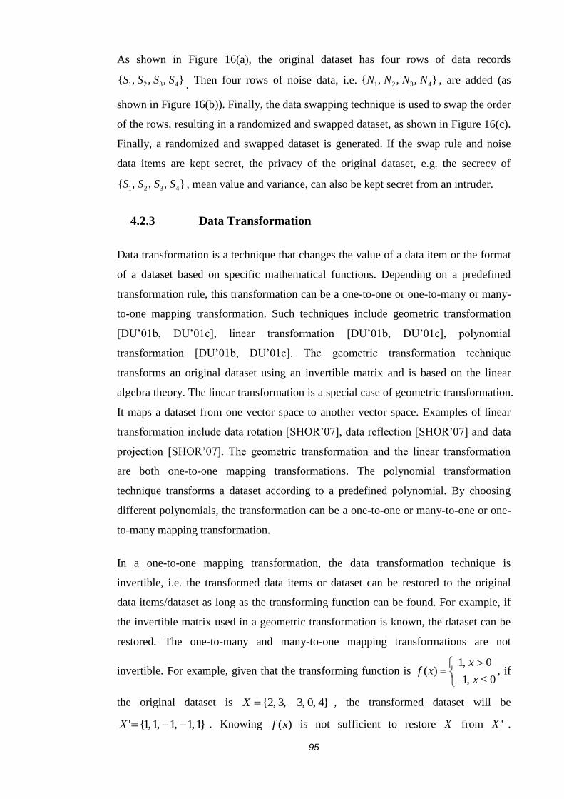
95

As shown in Figure 16(a), the original dataset has four rows of data records

},,,{ 4321 SSSS . Then four rows of noise data, i.e. },,,{ 4321 NNNN , are added (as

shown in Figure 16(b)). Finally, the data swapping technique is used to swap the order

of the rows, resulting in a randomized and swapped dataset, as shown in Figure 16(c).

Finally, a randomized and swapped dataset is generated. If the swap rule and noise

data items are kept secret, the privacy of the original dataset, e.g. the secrecy of

},,,{ 4321 SSSS , mean value and variance, can also be kept secret from an intruder.

4.2.3 Data Transformation

Data transformation is a technique that changes the value of a data item or the format

of a dataset based on specific mathematical functions. Depending on a predefined

transformation rule, this transformation can be a one-to-one or one-to-many or many-

to-one mapping transformation. Such techniques include geometric transformation

[DU’01b, DU’01c], linear transformation [DU’01b, DU’01c], polynomial

transformation [DU’01b, DU’01c]. The geometric transformation technique

transforms an original dataset using an invertible matrix and is based on the linear

algebra theory. The linear transformation is a special case of geometric transformation.

It maps a dataset from one vector space to another vector space. Examples of linear

transformation include data rotation [SHOR’07], data reflection [SHOR’07] and data

projection [SHOR’07]. The geometric transformation and the linear transformation

are both one-to-one mapping transformations. The polynomial transformation

technique transforms a dataset according to a predefined polynomial. By choosing

different polynomials, the transformation can be a one-to-one or many-to-one or one-

to-many mapping transformation.

In a one-to-one mapping transformation, the data transformation technique is

invertible, i.e. the transformed data items or dataset can be restored to the original

data items/dataset as long as the transforming function can be found. For example, if

the invertible matrix used in a geometric transformation is known, the dataset can be

restored. The one-to-many and many-to-one mapping transformations are not

invertible. For example, given that the transforming function is

0,1

0,1)(

x

xxf , if

the original dataset is }4,0,3,3,2{ X , the transformed dataset will be

}1,1,1,1,1{' X . Knowing )(xf is not sufficient to restore X from 'X .

96

Moreover, if )(xf is defined as

0,1

0

0,0

1

)(

x

x

xf , the transformed dataset 'X will

be

01100

10011'X , the format of the dataset is also changed.

4.3 Cryptographic Primitives

A cryptographic primitive is a well-established cryptographic algorithm that can be

used to construct computer security systems. This subsection describes cryptographic

primitives that are used in the design of our solutions.

The following cryptographic terms and definitions are used in the description in this

section and the remaining part of this thesis. Plaintext denotes a message in a readable

form, where a message can be any data that we may want to transfer. Message

encryption is a process of disguising a plaintext message to hide its meaning. An

encrypted message is referred to as ciphertext. Message decryption is a reverse

process of transforming a ciphertext into its original form. Encryption and decryption

are performed through the use of a cryptographic algorithm and a cryptographic key.

A key is typically a large random number, chosen from a pool of possible values

called key space. A cryptosystem is a system performing encryption and decryption

operations. In addition to encryption and decryption algorithms, it also has a range of

algorithms for key generation.

4.3.1 Additively Homomorphic Cryptosystem

Homomorphic Encryption

Homomorphic encryption is a form of encryption where a specific algebraic operation

performed on the plaintext is equivalent to another algebraic operation performed on

the ciphertext where the operation performed on the plaintext can be different from

the operation performed on the ciphertext. Homomorphic encryption schemes are

malleable by design. The homomorphic properties of various cryptosystems have

been applied in a variety of research topics [DAMG’03, RAPP’04], such as secure

voting systems, collision-resistant hash functions, and private information retrieval

97

schemes. In recent years, they have also been widely used in cloud computing to

ensure the confidentiality of the processed data [MICC’10].

A cryptosystem which supports only one algebraic operation is classified as a partially

homomorphic cryptosystem. Examples of partially homomorphic cryptosystem

include RSA cryptosystem [MENE’01], EIGamal cryptosystem [MENE’01], Benaloh

cryptosystem [BENA’94] and Paillier cryptosystem [PAIL’99a]. These cryptosystems

are described below.

- RSA Cryptosystem [MENE’01]

In the RSA cryptosystem, assuming that p and q are two large random and distinct

prime numbers, then pqn and )1)(1()( qpn . Select a random integer e

where )(1 ne , such that 1))(,gcd( ne . Compute d using the Extended

Euclidean algorithm where )(1 nd , such that ))((mod1 ned , i.e.

))((mod1 ned ; d is the multiplicative inverse of )(mod ne . The public

key consists of n and e , i.e. ),( enpk and the private key is d , i.e. dsk . Then

the encryption of a message x is given by computing nxxE e

pk mod)( . Its

homomorphic property is shown as follows:

)(mod)(mod)()( 21212121 xxEnxxnxxxExE pk

eee

pkpk .

The output of performing a multiplication on two ciphertexts is equivalent to the

output of encrypting the result of performing a multiplication on their original

plaintexts. As the RSA cryptosystem has the multiplicative property, it is classified as

a multiplicatively homomorphic cryptosystem.

- EIGamal Cryptosystem [MENE’01]

In the EIGamal cryptosystem, assuming that p is a large random prime number, is

a generator of the multiplicative group *

p of the integers modulo p and a is a

random integer where 21 pa . Then, the public key is ),,( ap , i.e.

),,( appk and the private key is a , i.e. ask . By randomly selecting an

integer k where 21 pk , the encryption of a plaintext x is given by computing

98

pk mod and px ka mod)( . ( is a parameter for decryption.) Its

homomorphic property is given as follows:

21

2121

21mod)()(mod))(())(( 2121

xx

kkakaka

xx pxxpxx

.


output of encrypting the result of performing a multiplication on their original

plaintexts. As the EIGamal cryptosystem has the multiplicative property, it is

classified as a multiplicatively homomorphic cryptosystem.

- Beneloh Cryptosystem [BENA’94]

In the Beneloh cryptosystem, assuming that the blocksize is r , p and q are two

large random prime numbers where r divides )1( p , 1)1

,gcd(

r

pr and

1)1,gcd( qr . Then pqn . Select }1),gcd(:{* nxZxy nn such that

1mod

)1)(1(

ny r

qp

. The public key is ),( ny , i.e. ),( nypk , and the private

key is ),( qp i.e. ),( qpsk . By randomly and uniformly selecting an u where

*

nu , the encryption of a message x is given by computing

nuyxE rx

pk mod)( . Its homomorphic property is shown as follows:

)(

mod)()(mod)()()()(

21

2121212121

xxE

muuymuyuyxExE

pk

rxxrxrx

pkpk

.


output of encrypting the result of performing an addition on their original plaintexts.

As the Beneloh cryptosystem has the additive property, it is classified as an additively

homomorphic cryptosystem.

- Paillier Cryptosystem [PAIL’99a]

In the Paillier cryptosystem, assuming that p and q are two large random prime

numbers such that 1))1)(1(,gcd( qppq . Compute pqn and

))1(),1(()( qplcmn . Select a random integer g where *

2ng such that n

99

divides the order of g . (This can be ensured by checking the multiplicative inverse ,

where nngL n mod))mod(( 12)( ) and L is defined as n

uuL

1)(

.) The

public key consists of n and g , i.e. ),( gnpk and the private key consists of

)(n and , i.e. )),(( nsk . By randomly selecting a r where *

nr , the

encryption of a message x is given by computing 2mod)( nrgxE nx

pk . Its

homomorphic property is shown as follows:

)(

mod)()(mod)()()()(

21

2

21

2

21212121

xxE

nrrgnrgrgxExE

pk

nxxnxnx

pkpk

.


output of encrypting the result of performing an addition on their original plaintexts.

As the Paillier cryptosystem has the additive property, it classified as an additively

homomorphic cryptosystem.

Assuming that 1m and 2m are two plaintexts and ))(),(,,( skpk DEskps is a

homomorphic cryptosystem, Figure 17 illustrates this homomorphic eproperty.

Figure 17. The homomorphic cryptosystem. (Source: Author’s own)

Each of the examples listed above allows homomorphic computation of only one

operation (either addition or multiplication) on plaintexts. A cryptosystem which

100

supports both additively and multiplicatively homomorphic properties is known as

fully homomorphic cryptosystem and is far more powerful [GENT’09]. Using such a

scheme, any circuit can be evaluated homomorphically, effectively allowing the

construction of programs. These programs can be run on encryptions of their inputs to

produce an encryption of their output. Since such a program does not need to decrypt

its input, it can be run by an un-trusted party without revealing its inputs and

computation details. The existence of an efficient and fully homomorphic

cryptosystem would have practical implications in the outsourcing of private

computations, for example, in the context of cloud computing [GENT’09].

Additively Homomorphic Encryption

In this thesis, we utilise the additively homomorphic property in the design of one of

our solutions, i.e. the P22NSTC protocol suite. We use the following property:

)()()( yxEyExE pkpkpk and yxyxED pksk ))(( . This allows us to conduct

an additive operation on encrypted data items without decrypting them. For example,

in a two-party computation with the assistance of a semi-trusted third party (STTP),

Alice and Bob negotiate an additively homomorphic encryption scheme, i.e.

))(),(,,( skpk DEskpk where pk is the public key, sk is the private key, )(pkE is

the encryption algorithm and )(skD is the decryption algorithm, prior to the

computation. Alice encrypts her private data x and generates )(xEpk ; Bob encrypts

his own private data y and generates )(yEpk . Alice and Bob then send )(xEpk and

)(yEpk to the STTP, respectively. The STTP can then calculate

)()()( yxEyExE pkpkpk and send )( yxEpk back to Alice and Bob. This

property preserves the privacy of x and y , preventing them from being disclosed to

the STTP, while ensuring that the STTP can calculate the desired result by performing

the multiplication operation on the encrypted data items.

Paillier Cryptosystem [PAIL’99a]

As the design of the P22NSTC protocol suite needs the additive property of the

additively homomorphic cryptosystem and the Paillier cryptosystem is regarded as the

most efficient additively homomorphic cryptosystem among its kind [CATA’01,

AKIN’09], it has been chosen to be employed in the implementation of the P22NSTC

101

protocol suite. Assuming that a party Alice constructs a Paillier cryptosystem, the

detail of this cryptosystem is described below.

- Key generation

1. To generate a key pair, Alice chooses two large secret prime numbers p and q ,

such that 1))1)(1(,gcd( qppq .

2. Alice sets pqn and computes ))1(),1(()( qplcmn .

3. Alice selects a random integer g , where *2n

g .

4. Alice checks the existence of nngL n mod))mod(( 12)( (the modular

multiplicative inverse), where L is defined as n

uuL

1)(

, to ensure that n

divides the order of g .

5. The public key (i.e. pk ) is ),( gn .

6. The private key (i.e. sk ) is )),(( n .

- Encryption

1. Let m be a message to be encrypted where nm .

2. Alice selects a random r where *

nr .

3. Alice computes the ciphertext of m , i.e. c , as follows:

2mod)( nrgmEc nm

pk .

- Decryption

1. The ciphertext *

2nc .

2. Alice recovers the plaintext m by computing

nngL

ncL

nncLcDm

n

n

n

sk

mod)mod(

)mod(

mod)mod()(

2)(

2)(

2)(

.

102

- Additively homomorphic property

1. Let 1m and 2m be two plaintexts.

2. the additively homomorphic property is:

)(

mod))((

mod))(()()(

21

2

21

2

2121

21

21

mmE

nrrg

nrgrgmEmE

pk

nmm

nmnm

pkpk

.

And

))(())()(( 212121 mmEDmmmEmED pkskpkpksk .

4.4 A Comparison of Privacy-preserving Building Blocks

Figure 18. A comparison of privacy-preserving building blocks. (Source: Author’s own)

Figure 18 compares the main features of the four privacy-preserving building blocks

described in this chapter. This comparison is done by comparing the building blocks

using the following six criteria:

(1) Does this building block change the values of the data items?

103

(2) Does this building block change the order of the data items?

(3) Does this building block change the format of the data items?

(4) Is this privacy-preserving operation reversible?

(5) The computational effort.

(6) The security level.

When the data swapping technique is applied to a dataset, it only changes the order of

the data items in the dataset. Neither the values nor the format of the data items is

changed. The technique can only provide a low level of security protection on dataset

reordering. As the swap operation is performed based on a pre-specified order, it is

reversible. It can be seen as a dataset which has been reordered by a permutation

matrix. Every permutation matrix is invertible. As the data swapping operation only

involves one matrix operation, the computational cost of this technique is low.

Noise data item addition randomization technique adds a large quantity of noise data

items into a dataset. It aims to hide the original data items in the noise data items. The

computational efforts required and the security level provided by this technique

depend on the number of noise data items it generates and adds into the original

dataset. It can be observed that if the number of noise data items is small, the

computational effort will be less. In addition, if the number of noise data items is

small in relation to the number of data items in the original dataset, the security

protection level will be corresponding low. A higher level of protection requires the

addition of more noise data items which will impose more computational effort. This

technique is often employed together with the data swapping technique.

Noise value addition randomization technique adds a random noise value to every

data item in the original dataset. The computational effort only involves noise value

generation and noise value addition. The security protection level is dependent on the

confidentiality of the noise value generation function. Once the function is known,

this operation can easily be reversed.

Data transformation technique can change both the value and format of data items

depending on the transformation functions used. If the transformation function is a

104

one-to-one mapping function, the transformation result is reversible. However, if the

transformation function is a one-to-many or many-to-one function, the transformation

result may not be reversible. The computational effort of the data transformation

technique depends on the transformation operations. If a more complicated function is

used, a higher computational effort is needed and a better level of protection is

provided.

Additively homomorphic cryptosystem changes the values and format of the data

items to be protected. It provides the best level of security protection among these

privacy-preserving building blocks. As the encryption/decryption operations are much

more complicated than normal algebraic operations, it also consumes the highest

computational effort.

4.5 Chapter Summary

This chapter has presented the privacy-preserving building blocks that form the basis

for the design of our two-party based and STTP based protocol suites. The first

protocol suite, i.e. the P22NSTP protocol suite, using a two-party based approach,

makes use of five novel building blocks that are designed based on the three data

perturbation techniques. The second solution, i.e. the P22NSTC protocol suite, using

the STTP based approach, is built on three novel building blocks that are designed

based on the three perturbation techniques and a cryptographic primitive. The details

of these protocol suites designs will be presented in chapter 5 and chapter 6,

respectively.

105

Chapter 5 A Novel Privacy-preserving Two-party

Nonparametric Sign Test Protocol Suite

Using Data Perturbation Techniques

(P22NSTP)


This chapter details the design of the P22NSTP protocol suite. Based on the design, the

security threats against privacy requirements are analysed. The correctness, the level

of the privacy it provides, the computational overhead and communication overhead

are also theoretically analysed in this chapter. The overview of the P22NSTP protocol

suite is described in section 5.2. Section 5.3 presents the detailed design, including

computation participants, message objects, components of the P22NSTP protocol suite

and elements of the computation. Finally, section 5.4 describes the operation of this

protocol and discusses the correctness, its privacy performance, computational

overhead and communication overhead.

5.2 Overview of the P22NSTP Protocol Suite

This protocol suite is designed for two parties, Alice and Bob, to collaboratively

perform the sign test computation while preserving the individual data confidentiality,

individual privacy and corporate privacy of X and Y . According to the design

requirements specified in chapter 3, this privacy-preserving sign test computation is

divided into four local computation tasks; each local computational task is carried out

by a specific protocol (or specific protocols) of the designed protocol suite. The data

perturbation techniques that have been selected in chapter 4 are used to preserve the

data privacy while supporting the computation of a task to be carried out. The

P22NSTP protocol suite consists of five components:

(1) The Random Probability Density Function Generation Protocol (RpdfGP).

(2) The Data Obscuring protocol (DOP).

(3) The Secure Two-party Comparison Protocol (STCP).

106

(4) The Data Extraction Protocol (DEP).

(5) The permutation reverse protocol (PRP).

The RpdfGP is employed by DOP and STCP as a function to generate a randomised

probability density function (pdf) during the protocol execution. This pdf is then used

to randomly generate noise data items by both of the protocols. The remaining four

protocols each performs a local computational task that is generated from the

decomposition of the sign test computation on an ideal trusted third party model

(TTP-NST). The detailed operations and their corresponding computational tasks are

described below.

Local Computational Task 1 - DOP

Assuming that Alice initiates a P22NSTP computation. Alice first executes DOP. DOP

is designed to protect the individual privacy and corporate privacy of X at the first

stage of the P22NSTP computation. DOP employs RpdfGP, data swapping and data

randomization techniques to generate a randomised data matrix MdTTX12

' . The

confidentiality of X is then disguised and concealed by MdTTX12

' . MdTTX12

' is sent to

Bob and used as one of the data inputs of STCP. (Assuming that the size of X is n ,

and 'n is the level of noise item addition managed by Alice, then MdTTX12

' is a matrix

of dimension )'()'( nnnn .)

Local Computational Task 2 - STCP

After receiving MdTTX12

' from Alice, Bob executes STCP to securely compare X and

Y without learning X . STCP employs RpdfGP, data swapping, data randomization

and data transformation techniques, to generate )'( nn disguised matrices, i.e. igDTU 3 ,

for )'(...,,1 nni . ( 'n is the level of noise item addition in MdTTX12

' , and it is

generated by Alice. Once Bob has received MdTTX12

' , he can know the dimension of

MdTTX12

' , i.e. )'()'( nnnn . As Bob knows the value of n , he can find out the

value of 'n by computing nnn )'( .) More specifically, STCP protects individual

data confidentiality, individual privacy and corporate privacy of Y . The corporate

privacy of the joint dataset, i.e. the intermediate computation result },,{ RQP is also

107

protected and concealed by these )'( nn disguised matrices. These )'( nn matrices

will be sent to Alice and used as the data input of DEP.

Local Computational Task 3 - DEP

After receiving 1

)'(}{ 3

i

nn

gDT iU from Bob, Alice executes DEP to reverse the data

disguising effects in 1

)'(}{ 3

i

nn

gDT iU that are imposed by DOP. In addition, DEP

computes all possible sign test results in relation to 1

)'(}{ 3

i

nn

gDT iU , i.e. 1

)1)(2)(3(}{

i

lll

I

idc

and 1

)1)(2)(3(}{

i

lll

T

iR , where dI

ic is an index of a combination (there are

)1)(2)(3( lll combinations in total) and T

iR is the test result in relation to dI

ic ,

for )1)(2)(3(...,,1 llli . 1

)1)(2)(3(}{

i

lll

I

idc and

1

)1)(2)(3(}{

i

lll

T

iR will be sent to Bob

and used as the data input of PRP.

Local Computational Task 4 - PRP

Finally, Bob executes PRP to single out the final test result, i.e. finalTR , from

1

)1)(2)(3(}{

i

lll

T

iR . Bob then sends the final test result finalTR to Alice.

Figure 19 provides an overview of the P22NSTP execution.

Figure 19. An overview of the P22NSTP computation.

(Source: Author’s own)

108

5.3 The Design in Detail

It can be seen from Figure 19 that after the execution of each of the local

computational tasks, an intermediate computational result is generated. This

intermediate computation result will be later transmitted to the other party along with

further data (detailed in subsection 5.3.1), and used as the input of the next local

computation task. At the last stage of the computation, the final result is generated by

Bob and then sent to Alice. To summarise, four messages are transmitted during the

P22NSTp protocol suite execution. The following subsections present the design

details of the P22NSTP protocol suite.

5.3.1 Computation Participants and Message Objects

Computation Participants:

There are two participants, Alice and Bob. Alice holds dataset X , and Bob holds

dataset Y , where }...,,{ 1 nxxX , }...,,{ 1 nyyY and X and Y are vertically

partitioned.

Message Objects:

The execution of this protocol suite consists of four local computations. Assuming

that Alice initiates the computation. Four message objects are transferred during the

computation, which are:

Message 1: Alice sends Bob the output of DOP, i.e. )(XDOP , and 1T , where

)(XDOP = MdTTX12

' . 1T is a permutation matrix generated by Alice. That

is, },'{ 11 12TXmsg MdTT .

MdTTX12

' and 1T are both matrices of dimension )'()'( nnnn .

Message 2: Bob sends Alice the output of STCP, i.e. ),,'( 112TYXSTCP MdTT , where

1

)'(1 }{),,'( 2

12

i

nn

gDT

MdTTiUTYXSTCP . That is, }}{{ 1

)'(22

i

nn

gDT iUmsg .

igDTU 2 is a matrix of dimension )'()3( nnl . There are )'( nn

matrices in 2msg .

109

Message 3: Alice sends Bob the output of DEP, i.e. ),}({ 2

1

'2 Ri

nn

gDTTabUDEP i

, where

}}{,}{{),}({ 1

)3)(2)(1(

1

)3)(2)(1(2

1

'2

i

lll

T

i

i

lll

I

i

Ri

nn

gDTRcTabUDEP di . That is,

}}{,}{{ 1

)3)(2)(1(

1

)3)(2)(1(3

i

lll

T

i

i

lll

I

i Rcmsg d .

dI

ic is a vector of dimension 31 . T

iR is an integer value and T

iR is

either “0” or “1”, where “0” represents “do not reject 0H ” and “1”

represents “reject 0H ”. T

iR is the computational result in relation to

dI

ic . There are )1)(2)(3( lll vectors and )1)(2)(3( lll integer

values in 3msg .

Message 4: Bob sends Alice the output of PRP,

i.e. ),}{,}({ 3

1

)3)(2)(1(

1

)3)(2)(1(

Ri

lll

I

i

i

lll

T

i TabcRPRP d

,

where final

Ri

lll

I

i

i

lll

T

i TRTabcRPRP d

),}{,}({ 3

1

)3)(2)(1(

1

)3)(2)(1( .

That is, }{4 finalTRmsg .

finalTR is an integer value. There is only one integer value data item in

4msg .

5.3.2 Components of the P22NSTP Protocol Suite

The five novel components are detailed below.

5.3.2.1 Random Probability Density Function Generation Protocol (RpdfGP)

RpdfGP is designed for a party (Alice and Bob, respectively) to randomly generate a

Probability Density Function (pdf) based on their respective original dataset. This

random pdf will then be used by the parties to further generate noise data items to

disguise their original datasets. By adding a large number of noise data items, the

individual privacy and the corporate privacy of the original dataset can be protected.

In the case of Alice executing this protocol, it can be detailed as follows.

110

Random Probability Density Function Generation Protocol (RpdfGP)

Input: ]...,,[ 11 nn xxX .

Output: )(mf .

(1) Calculate n

xn

i i

x

1 .

(2) Calculate n

xn

i xi

x

)(12

.

(3) Calculate }{maxmax ii

xx .

(4) Calculate }{minmin ii

xx .

(5) Randomly generate three integers, 1k , 2k and 3k , from )100,1(U .

(6) Randomly generate 'x from ),0( 1 xkU .

(7) Randomly generate 2

'x from ),0( 2

2 xkU .

(8) Randomly generate min'x from ),0( minxU .

(9) Randomly generate max'x from ),0( max3 xkU .

(10) Randomly select )(mf from the pdf of ),( 2

'' xxN or the pdf of

)','( maxmin xxU , with probability 2

1.

(11) Output )(mf .

Figure 20. The RpdfGP algorithm. (Source: Author’s own)

The rationales of key computation steps in Figure 20 are explained below.

In step (5), 1k , 2k and 3k are security parameters managed by the protocol

executor. They are later used in step (6), (7) and (9) to generate 'x , 2

'x and

max'x , respectively. 1k is randomly drawn from )100,1(U . This ensures that 'x

can be randomly drawn from a wider interval, i.e. an interval between 0 and

xk 1 . This increases the randomness of 'x and the noise data items

),( 2

'' xxN generates. 2k is randomly drawn from )100,1(U , and this ensures

that 2

'x can be randomly drawn from a wider interval, i.e. an interval between 0

and 2

2 xk . This increases the randomness of 2

'x and the noise data items

111

),( 2

'' xxN generates. 3k is randomly drawn from )100,1(U , and this ensures

that max'x can be randomly drawn from a wider interval, i.e. an interval between

0 and max3 xk . This increases the randomness of max'x and the noise data items

)','( maxmin xxU generates. The function ),( baU is a configurable security

parameter that is managed by Alice. By controlling a and b , a specific level of

security can be achieved.

In step (10), randomly selecting )(mf from ),( 2

'' xxN and )','( maxmin xxU is

also a way of increasing the randomness of noise data item generation. By using

this method, the random noises from )(mf can be generated either from

),( 2

'' xxN or )','( maxmin xxU with the probability of 2

1. (The list of pdf

candidates is also managed by the protocol executor. For example, )(mf can be

chosen from nfff ...,,, 21 with the probability of n

1, where nfff ...,,, 21 are n

different functions.)

How the corporate privacy of nX 1 is preserved.

The output of RpdfGP is a pdf, and this pdf is either a normal distribution function or

a uniform distribution function. It contains disguised information about the original

dataset. This protocol will be employed by both Alice and Bob to generate noise data

items to conceal X and Y , respectively. As this pdf is generated by increasing the

value range of the original dataset, it becomes more difficult to distinguish the

original data items from the resulting randomised dataset. For example, after Alice

executes this protocol and generates )(mf , )(mf will then be used to generate a

large number of noise data items to the randomised dataset in the next stage of

computation. Despite whatever features the original dataset holds, if an intruder wants

to know the information about X and has collected as many data items as he/she can,

the corporate privacy that can be inferred from the randomised dataset directly is

either ),(~ 2

'' xxNX or )','(~ maxmin xxUX , where 'x , 2

'x , min'x and max'x have

112

all been randomised. The corporate privacy of X , for example, the distribution

properties, can be concealed by these random values generated by )(mf .

5.3.2.2 Data Obscuring Protocol (DOP)

The data obscuring protocol (DOP) is designed to protect the confidentiality of an

original dataset at the first stage of the P22NSTP execution. RpdfGP, data

randomization and data swapping techniques are employed in DOP. By using RpdfGP,

a managed number of noised data items are generated. These noise data items and the

original dataset are merged into a bigger dataset. This dataset is then swapped using a

random permutation matrix, i.e. a permutation matrix. The individual privacy and

corporate privacy of the original dataset can then be preserved. Assuming that Alice

executes this protocol, it can be detailed as follows.

Data Obscuring Protocol (DOP)

Input: nX 1 .

Output: MdTTX12

' .

(1) Execute RpdfGP to generate a random pdf )(mf A .

(2) Generate a random integer 4k from )100,1(U .

(3) Set nkn 4' .

(4) Use )(mf A to generate a random vector ]...,,[ '1 naug aaX , where )(~ mfa Ai .

(5) Merge X and augX to produce 'X , where ]...,,,...,,[' '11 nn aaxxX .

(6) Generate a permutation matrix 1T of dimension )'()'( nnnn .

(7) Compute 1''1

TXX T , assume ]'...,,'[' )'(11 nnT xxX .

(8) Generate a table CTab1 to record the swapping order for each ix ' in relation to jx

and ka , where )'(...,,1 nni , nj ...,,1 and '...,,1 nk .

(9) Transform 1

'TX to a diagonal matrix, 1

'dTX , of dimension )'()'( nnnn , i.e.

)'(

2

1

'00

0'0

00'

'1

nn

dT

x

x

x

X

.

(10) Generate a random matrix M of dimension )'()'( nnnn by using )(mf A

in the following manner: assuming that the elements of M are ijm , where

)'(...,,1 nni and )'(...,,1 nnj . 0ijm for ji ; for ji , ijm are

values randomly generated from )(mf A .

(11) Generate a randomised dataset matrix, MdTX1

' , by computing

113

MXX dTMdT 11

'' .

(12) Randomly generate a permutation matrix 2T of dimension )'()'( nnnn .

(13) Swap the row order of MdTX1

' by computing MdTMdTT XTX112

'' 2 .

(14) Generate a table RTab2 to record the indices of every ix' in MdTTX12

' , for

)'(...,,1 nni .

Figure 21. The DOP algorithm. (Source: Author’s own)

The rationales of key computation steps and the formats of the computational

elements in Figure 21 are described below.

In step (2), 4k is a security parameter managed by Alice. It is later used in step (3)

to generate 'n , i.e. the noise addition level of MdTTX12

' . As nkn 4' and 4k is

randomly drawn from )100,1(U , the number of noise data items to be added is

also random and is at least nk 4 . The larger the 4k , the more the number of

noise data items are to be added. Consequently, more computational effort will

be needed to process the disguised dataset. The probability function ),( baU is a

configurable security parameter that is managed by Alice. By controlling a and

b , a desired level of security can be achieved.

In steps (4) - (5),

assuming that and ,

then .

'X is the dataset that contains original data items and noise data items. The

column order of the data items in 'X has not been swapped.

114

In steps (6) - (8),

assuming that the permutation matrix

)'()'(

1

0010

0001

0100

1000

nnnn

T

,

then ,

and .

1T swaps the column order of the data items in 'X . CTab1 records the change of

the column orders caused by 1T .

The purpose of using augX and 1T is to prevent the sample size of X and Y

from being learnt by external attackers. In a P22NSTP computation, although the

messages are assumed to be transferred via secure channels, there is still a

possibility that external attackers might breach the channels and get the messages.

In such a case, external attackers may hold the same information as Alice and

Bob, except the size of X and Y . If external attackers do not know the size of

the original dataset, it would be more difficult for them to restore the original

dataset. The use of 1T can preserve the corporate privacy of X and Y against

external attackers throughout the P22NSTP computation. If the possibility of

external attackers is a concern, the use of augX and 1T may not be necessary.

115

In steps (9) - (11), by using 1

'TX , the details of 1

'dTX and MdTX1

' are illustrated as

follows:

and .

In steps (12) - (14), assuming that the permutation matrix

)'()'(

2

0001

0010

0100

1000

nnnn

T

,

then ,

and .

2T swaps the row order of the rows in MdTX1

' . RTab2 records the changes of the row

orders caused by 2T .

116

How privacy is preserved.

As in a vertically partitioned data model, the two parties are dealing with an identical

set of data subjects, the identities of which are implied by the dataset and may already

be known to both Alice and Bob. One way to preserve the individual privacy in such a

data model is to make the inference of the match up between a certain data item and

the identity of the subject of the data item as difficult as possible. The level of

difficulty for Bob to infer the identity of the subject to whom a specific data item

managed by Alice is associated is dependent on the sample size, n . The larger the

sample size, the higher the level of difficulty. As the random noise data items are

generated by )(mf A , the original data items of X can not be distinguished from

noise data items after being mixed with them. Alice can control the level of difficulty

by managing the size of 'n . This protocol adds nnn 2)'( noise data items to 1

'dTX

so as to generate the randomised matrix MdTX1

' . In addition, MdTX1

' is further

permuted using 2T so as to generate MdTTX12

' . If curious Bob wants to infer X from

MdTTX12

' , he would have to figure out the real value of 2T . The probability for Bob to

successfully guess 2T is )!'(

1

nn , which is negligible when 'n is sufficiently large in

relation to n .

5.3.2.3 Secure Two-party Comparison Protocol (STCP)

The secure two-party comparison protocol (STCP) is designed to allow one of the two

parties to compare the two datasets without learning either the exact values of the

other party’s dataset or the comparison results. In addition to RpdfGP, data

randomization and data swapping techniques, data transformation technique is used in

this protocol to preserve the difference of each pairwised comparison. STCP is

executed by Bob after Alice executes DOP. It compares his private dataset Y with

Alice’s private dataset X , while the individual privacy of Y and the corporate

privacy of the comparison results, i.e. },,{ RQP , are preserved. The detailed

description of this protocol is given below.

117

Secure Two-party Comparison Protocol (STCP)

Input: MdTTX12

' and 1T (from Alice); nY 1 from Bob.

Output: 1

)'(}{ 13

i

nn

gDTU .

(1) Execute RpdfGP to generate a random pdf )(efB .

(2) Use )(efB to generate a random vector, ]...,,[ '1 naug eeY , where )(~ efe Bi .

(3) Merge Y with augY to generate ],...,,...,,[' '11 nn eeyyY .

(4) Compute 1''1

TYY T . For the sake of clarity, we assume ]'...,,'[' )'(11 nnT yyY .

(5) Generate a matrix 1'' TYY of dimension )'()'( nnnn , where

)'(21

)'(21

)'(21

'

'''

'''

'''

'1

nn

nn

nn

TY

yyy

yyy

yyy

Y

.

(6) Compute 112 ''' TYMdTT YXD , where D is the comparison result matrix. We

assume

)')('(2)'(1)'(

)'(22221

)'(11211

nnnnnnnn

nn

nn

ddd

ddd

ddd

D

and the row vectors of D are

1D , …, )'( nnD , i.e. ]...,,[ )'(1111 nnddD , …, ]...,,[ )')('(1)'()'( nnnnnnnn ddD . Here

D indicates the result of MdTTX12

' subtracting 1'' TYY ; iD indicates the results of

the thi row of MdTTX12

' subtracting 1

'TY , for )'(...,,1 nni .

(7) Generate a function )(dg such that

.0,

1

0

0

.0,

0

1

0

.0,

0

0

1

)(

d

d

d

dg

(8) Compute ))]((...,)),([()( )'(1 nniii dgdgDg , for )'(...,,1 nni . Here )( iDg is

the transformed comparison result of iD and it is a )'(3 nn data matrix.

(9) Generate a random integer 5k from )100,1(U .

(10) Set

33 5 nk

l .

(11) To disguise 1

)'()}({

i

nniDg , generate random matrices iU with dimension

)'( nnl , for )'(...,,1 nni , where the elements of iU are randomly

drawn from }1,0{ . These random matrices are generated so as to add random

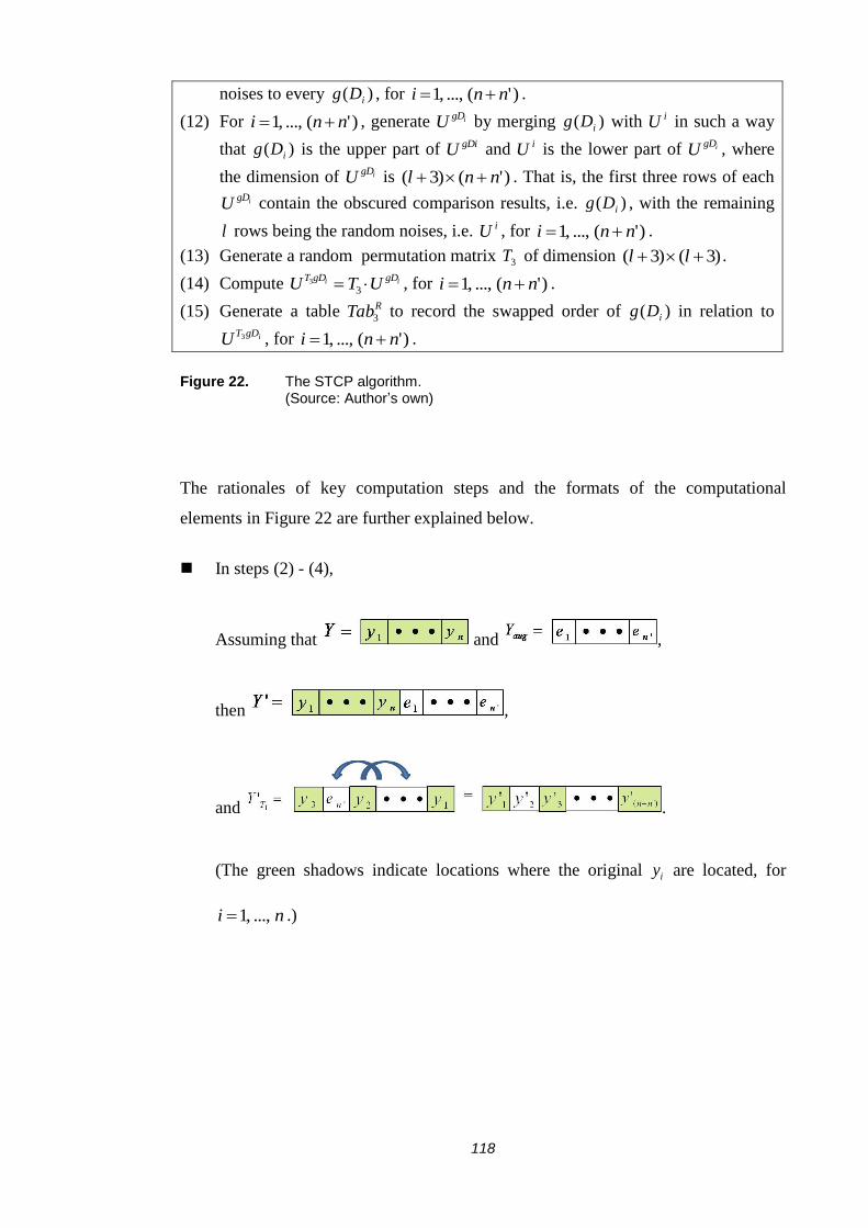
118

noises to every )( iDg , for )'(...,,1 nni .

(12) For )'(...,,1 nni , generate igDU by merging )( iDg with iU in such a way

that )( iDg is the upper part of gDiU and iU is the lower part of igDU , where

the dimension of igDU is )'()3( nnl . That is, the first three rows of each

igDU contain the obscured comparison results, i.e. )( iDg , with the remaining

l rows being the random noises, i.e. iU , for )'(...,,1 nni .

(13) Generate a random permutation matrix 3T of dimension )3()3( ll .

(14) Compute ii gDgDTUTU 3

3 , for )'(...,,1 nni .

(15) Generate a table RTab3 to record the swapped order of )( iDg in relation to

igDTU 3 , for )'(...,,1 nni .

Figure 22. The STCP algorithm. (Source: Author’s own)


elements in Figure 22 are further explained below.

In steps (2) - (4),

Assuming that and ,

then ,

and .

(The green shadows indicate locations where the original iy are located, for

ni ...,,1 .)

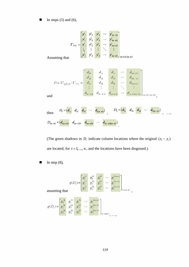
119

In steps (5) and (6),

Assuming that

and ,

then , , …,

.

(The green shadows in iD indicate column locations where the original )( ii yx

are located, for ni ...,,1 , and the locations have been disguised.)

In step (8),

assuming that ,

, …,

120

and after the data

transformation. The value of ij

kg is either 1, 0 or -1, for )'(...,,1 nni ,

)'(...,,1 nnj and )'(...,,1 nnk .

In step (9), 5k is a security parameter managed by Bob. It is later used in step

(10) to generate l , i.e. the noise row addition level of 1

)'(}{ 3

i

nn

gDT iU .

33 5 nk

l

and 5k is randomly drawn from )100,1(U , this ensures that the number of noise

rows to be added in every igDTU 3 is at least 5k times more than n and l . l can

also be divided by 3 (for explanation, here we further let 5'3kl ). This ensures

that the row vectors of every igDTU 3 can be separated into 5'k sets of },,{ RQP

combinations. The larger the 5k , the more the number of noise rows.

Consequently, more computational effort will be needed to process the disguised

dataset. The probability function ),( baU is a configurable security parameter

that is managed by Bob; a desired level of security can be achieved by

controlling a and b .

In step (11), assume

)'(

1

)'(

1

3

1

2

1

1

1

)'(3

1

33

1

32

1

31

1

)'(2

1

23

1

22

1

21

1

)'(1

1

13

1

12

1

11

1

nnlnnllll

nn

nn

nn

uuuu

uuuu

uuuu

uuuu

U

,

)'(

2

)'(

2

3

2

2

2

1

2

)'(3

2

33

2

32

2

31

2

)'(2

2

23

2

22

2

21

2

)'(1

2

13

2

12

2

11

2

nnlnnllll

nn

nn

nn

uuuu

uuuu

uuuu

uuuu

U

, …,

121

)'(

)'(

)'(

)'(

3

)'(

2

)'(

1

)'(

)'(3

)'(

33

)'(

32

)'(

31

)'(

)'(2

)'(

23

)'(

22

)'(

21

)'(

)'(1

)'(

13

)'(

12

)'(

11

)'(

nnl

nn

nnl

nn

l

nn

l

nn

l

nn

nn

nnnnnn

nn

nn

nnnnnn

nn

nn

nnnnnn

nn

uuuu

uuuu

uuuu

uuuu

U

.

In step (12), assume

)'()3(

1

)'(

1

3

1

2

1

1

1

)'(3

1

33

1

32

1

31

1

)'(1

1

13

1

12

1

11

)'(1

3

13

3

12

3

11

3

)'(1

2

13

2

12

2

11

2

)'(1

1

13

1

12

1

11

1

1

nnlnnllll

nn

nn

nn

nn

nn

gD

uuuu

uuuu

uuuu

gggg

gggg

gggg

U

,

)'()3(

2

)'(

2

3

2

2

2

1

2

)'(3

2

33

2

32

2

31

2

)'(1

2

13

2

12

2

11

)'(2

3

23

3

22

3

21

3

)'(2

2

23

2

22

2

21

2

)'(2

1

23

1

22

1

21

1

2

nnlnnllll

nn

nn

nn

nn

nn

gD

uuuu

uuuu

uuuu

gggg

gggg

gggg

U

, …,

)'()3(

)'(

)'(

)'(

3

)'(

2

)'(

1

)'(

)'(3

)'(

33

)'(

32

)'(

31

)'(

)'(1

)'(

13

)'(

12

)'(

11

)')('(

3

3)'(

3

2)'(

3

1)'(

3

)')('(

2

3)'(

2

2)'(

2

1)'(

2

)')('(

1

3)'(

1

2)'(

1

1)'(

1

)'(

nnl

nn

nnl

nn

l

nn

l

nn

l

nn

nn

nnnnnn

nn

nn

nnnnnn

nnnnnnnnnn

nnnnnnnnnn

nnnnnnnnnn

gD

uuuu

uuuu

uuuu

gggg

gggg

gggg

U nn

.

In step (13), for illustration we let

)3()3(

3

0001

1000

0100

0010

ll

T

.

122

Then in step (14),

)'()3(

)'(1

1

13

1

12

1

11

1

1

)'(

1

3

1

2

1

1

)'(1

3

13

3

12

3

11

3

)'(1

2

13

2

12

2

11

2

13

nnl

nn

nnllll

nn

nn

gDT

gggg

uuuu

gggg

gggg

U

,

)'()3(

)'(2

1

23

1

22

1

21

1

2

)'(

2

3

2

2

2

1

)'(2

3

23

3

22

3

21

3

)'(2

2

23

2

22

2

21

2

23

nnl

nn

nnllll

nn

nn

gDT

gggg

uuuu

gggg

gggg

U

, …,

)'()3(

)')('(

1

3)'(

1

2)'(

1

1)'(

1

)'(

)'(

)'(

3

)'(

2

)'(

1

)')('(

3

3)'(

3

2)'(

3

1)'(

3

)')('(

2

3)'(

2

2)'(

2

1)'(

2

)'(3

nnl

nnnnnnnnnn

nn

nnl

nn

l

nn

l

nn

l

nnnnnnnnnn

nnnnnnnnnn

gDT

gggg

uuuu

gggg

gggg

U nn

.

Then in step (15),

.

This table records the change of row orders in every igDTU 3 , for )'(...,,1 nni .


Upon receipt of MdTTX12

' and 1T from Alice, Bob can compute T

MdTTdMT TXX 1122''

(T

T1 is the transpose matrix of 1T ) to reverse 1T ’s swap effect in MdTTX12

' . He can

then infer the real values of ix s using dMTX2

' . The probability for Bob to successfully

infer X is )1'()1')('(

1

nnnnn , it approximates

nnn )'(

1

as nn ' . This

probability is negligible when 'n is sufficiently large. The probability for Bob to

successfully infer the intermediate result },,{ RQP is the same as the probability of

inferring X . As Alice manages the security parameter 'n , the larger the value of 'n

the more difficult it is for Bob to infer X and },,{ RQP .

123

How random matrices nnUU '1 ...,, are chosen.

In this protocol, iU s are used to conceal the values of intermediate computation

results },,{ RQP in gDiU s. As nRQP , these iU s should be chosen in a such

way that the row sum of any three rows in each gDiU should be equal to )'( nn ,

otherwise the level of security would be lowered. This is because all these data

matrices, 1

)'(}{ 3

i

nn

gDT iU , will be sent to Alice at the next stage of computation. If some

row combinations with row sums not equal to )'( nn exist, the chance for Alice to

infer },,{ RQP from these matrices would be higher. (According to the nature of sign

test, the value of )( RQP should be equal to n . In a case when nRQP , it

is not valid for sign test computation.)

5.3.2.4 Data Extraction Protocol (DEP)

The data extraction protocol (DEP) is designed to reverse the data obscuring

operations performed on 1

)'(}{ 3

i

nn

gDT iU by DOP. It further computes the sign test results

on 1

)'(}{ 3

i

nn

gDT iU . Assuming that Alice executes this protocol, the protocol details can

be described as follows.

Data Extraction Protocol (DEP)

Input: RTab2 (from Alice);

1

)'(}{ 3

i

nn

gDT iU (from Bob)

Output: 1

)1)(2)(3(}{

i

lll

T

iR

(1) Use RTab2 to extract

'

)'(

'

1 ...,, x

nn

x VV from )'(313 ...,, nngDTgDTUU . Here

'

)'(

'

1 ...,, x

nn

x VV

are column vectors where ix' s are stored.

(2) Compute a )'()3( nnl data matrix Ud by merging '

)'(

'

1 ...,, x

nn

x VV , where

'x

iV is the thi column vector of Ud , for )'(...,,1 nni .

(3) Compute TddTTUU

T

11 .

(4) Divide UTdT1 into two parts, i.e. ]|[ 111 UUU

TTT dT

a

dT

x

dT , where U

TdT

x1 is a data

matrix of dimension nl )3( and UTdT

a1 is a data matrix of dimension

')3( nl .

(5) Calculate the column vector of the row sum of UTdT

x1 by computing

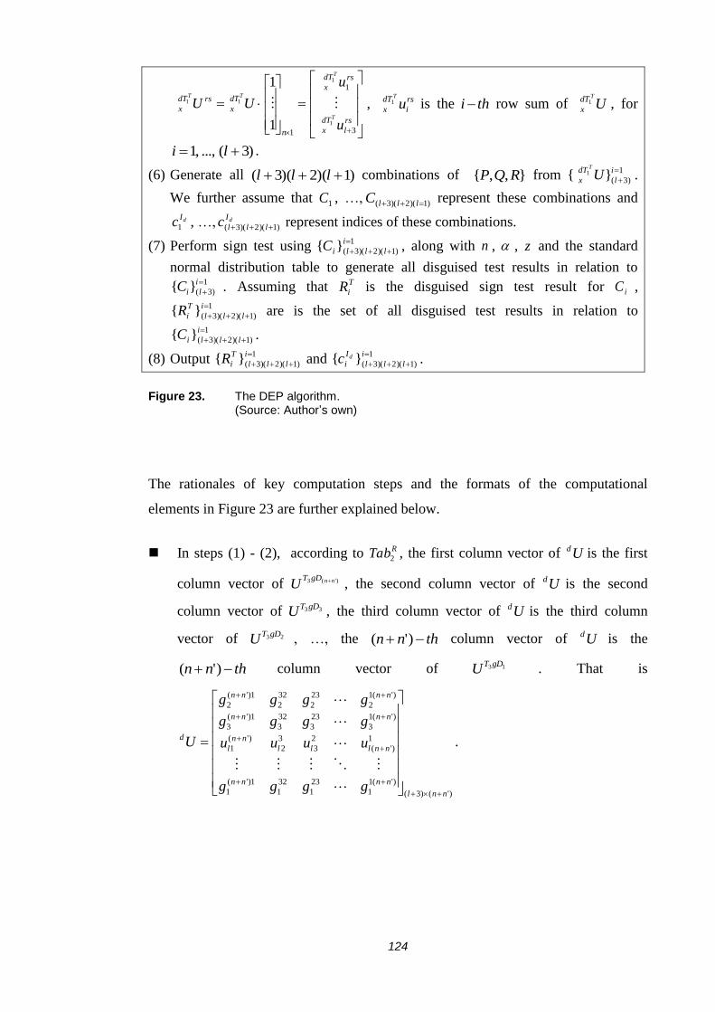
124

rs

l

dT

x

rsdT

x

n

dT

x

rsdT

x

u

u

UUT

T

TT

3

1

1

1

1

11

1

1

, rs

i

dT

x uT

1 is the thi row sum of UTdT

x1 , for

)3(...,,1 li .

(6) Generate all )1)(2)(3( lll combinations of },,{ RQP from 1

)3(}{ 1

i

l

dT

x UT

.

We further assume that 1C , …, )1)(2)(3( lllC represent these combinations and

dIc1 , …, dI

lllc )1)(2)(3( represent indices of these combinations.

(7) Perform sign test using 1

)1)(2)(3(}{

i

llliC , along with n , , z and the standard

normal distribution table to generate all disguised test results in relation to 1

)3(}{

i

liC . Assuming that T

iR is the disguised sign test result for iC ,

1

)1)(2)(3(}{

i

lll

T

iR are is the set of all disguised test results in relation to

1

)1)(2)(3(}{

i

llliC .

(8) Output 1

)1)(2)(3(}{

i

lll

T

iR and 1

)1)(2)(3(}{

i

lll

I

idc .

Figure 23. The DEP algorithm. (Source: Author’s own)


elements in Figure 23 are further explained below.

In steps (1) - (2), according to RTab2 , the first column vector of Ud is the first

column vector of )'(3 nngDTU , the second column vector of Ud is the second

column vector of 33gDTU , the third column vector of Ud is the third column

vector of 23gDTU , …, the thnn )'( column vector of Ud is the

thnn )'( column vector of 13gDTU . That is

)'()3(

)'(1

1

23

1

32

1

1)'(

1

1

)'(

2

3

3

2

)'(

1

)'(1

3

23

3

32

3

1)'(

3

)'(1

2

23

2

32

2

1)'(

2

nnl

nnnn

nnlll

nn

l

nnnn

nnnn

d

gggg

uuuu

gggg

gggg

U

.

125

In step (3),

as ,

then

)'()3(

32

1

1)'(

1

23

1

)'(1

1

3

2

)'(

1

2

3

1

)'(

32

3

1)'(

3

23

3

)'(1

3

32

2

1)'(

2

23

2

)'(1

2

1

nnl

nnnn

l

nn

llnnl

nnnn

nnnn

dT

gggg

uuuu

gggg

gggg

UT

.

In step (4),

assuming that

)')(3()1)(3()3(2)3(1)3(

)'(3)3(333231

)'(2)2(222221

)'(1)1(111211

1

nnlnlnlll

nnnn

nnnn

nnnn

dT

uuuuu

uuuuu

uuuuu

uuuuu

UT

,

then

nlll

n

n

n

dT

x

uuu

uuu

uuu

uuu

UT

)3(2)3(1)3(

33231

22221

11211

1

and

)')(3()1)(3(

)'(3)3(3

)'(2)2(2

)'(1)1(1

1

nnlnl

nnn

nnn

nnn

dT

a

uu

uu

uu

uu

UT

.

In step (5),

rs

l

dT

x

rsdT

x

rsdT

x

rsdT

x

n

i il

n

i i

n

i i

n

i i

n

dT

x

rsdT

x

u

u

u

u

u

u

u

u

UU

T

T

T

T

TT

)3(

3

2

1

1 )3(

1 3

1 2

1 1

11

1

1

1

11

1

1

1

1

,

where rs

i

dT

xuT

1 is the possible value for P , Q or R , for )3(...,,1 li .

126

In steps (6) - (8), the relationship among iC , Id

ic and T

iR is described in Figure 24.

Figure 24. The detailed relationship among iC , Id

ic andT

iR .



This protocol prevents Alice from knowing },,{ RQP and Y . The probability for

Alice to successfully guess },,{ RQP is )1)(2)(3(

1

lll and this probability

converges to 3

1

l. Bob can control the security level by increasing or decreasing the

value of l . The real values of differences between ix and iy have been transformed

to ),,( iii RQP , where }1,0{,, iii RQP , for )'(...,,1 nni . In the event where Alice

has successfully guessed },,{ RQP , she may still be able to work out Y . To

compromise the individual privacy of Y , Alice needs to work out if the data pairs in

the joint dataset YX are equal or not, i.e. Alice has to find the value of Q . The

probability for Alice to successfully guess these identical pairs is )!(

)!(!3 nl

QnQ

. For

those pairs of ii yx or ii yx , the only information Alice can work out is the

relative relations for each ),( ii yx , rather than the actual value of iy .

5.3.2.5 Permutation Reverse Protocol (PRP)

The permutation reverse protocol (PRP) is designed to reverse the result of the data

obscuring operations performed by STCP and to single out the final sign test result.

127

As we assume STCP is executed by Bob, here, PRP is also executed by Bob to

reverse the permutation effect of 3T in 1

)'(}{ 3

i

nn

gDT iU . This protocol can be detailed as

follows.

Permutation Reverse Protocol (PRP)

Input: 1

)1)(2)(3(}{

i

lll

I

idc and

1

)1)(2)(3(}{

i

lll

T

iR (from Alice); RTab3 (from Bob).

Output: The final sign test result finalTR .

(1) Find dI

Fc from 1

)1)(2)(3(}{

i

lll

I

idc using RTab3 , where dI

Fc is the index of actual

},,{ RQP

(2) Find finalTR from 1

)1)(2)(3(}{

i

lll

T

iR using dI

Fc .

Figure 25. The PRP algorithm. (Source: Author’s own)

In this final protocol, Bob uses RTab3 to reverse the permutation operation on

1

)'(}{ 3

i

nn

gDT iU that has been performed by STCP, thus identifying the final test result

from 1

)1)(2)(3(}{

i

lll

T

iR . Each T

iR represents the test result for the corresponding

possible combinations of },,{ RQP . 1

)1)(2)(3(}{

i

lll

I

idc are indices for

1

)1)(2)(3(}{

i

lll

T

iR .

By referring to RTab3 and 1

)1)(2)(3(}{

i

lll

I

idc , dI

Fc can be identified, thus finalTR can be

singled out from 1

)1)(2)(3(}{

i

lll

T

iR .The computation result of each T

iR is an integer

value, where 1T

iR represents “reject 0H ” and 0T

iR represents “do not reject

0H ”. As Bob does not know any information about how Alice produces this index,

the only way he can infer 1

)1)(2)(3(}{

i

lll

I

idc is by guessing. The probability for Bob to

infer 1

)1)(2)(3(}{

i

lll

T

iR is )1)(2)(3(

1

lll. At this point, it is virtually impossible for

Bob to infer any information about either X or },,{ RQP . In the case where Bob

correctly identifies the final test result but intentionally sends the wrong result to

Alice, although this computation has been compromised, the privacy of X and

},,{ RQP are still preserved.

128

5.4 The P22NSTP Protocol Suite and Its Operation

On the basis of the components described above, we can now construct the P22NSTP

protocol suite. Based on the assumption that Alice initiates this computation, the

protocol description is detailed in the following subsection.

5.4.1 Operation of the P22NSTP Protocol Suite

The P22NSTP Protocol Suite

Input: (1) X from Alice.

(2)Y from Bob.

(3) and z are negotiated and determined by both Alice and Bob.

Output: Both Alice and Bob obtain the final computation result.

(1) Alice executes DOP. (Input: X ; Output: MdTTX12

' .)

(2) Alice sends MdTTX12

' and 1T to Bob.

(3) Bob executes STCP. (Input: MdTTX12

' , Y and 1T ; Output: 1

)'(}{ 3

i

nn

gDT iU .)

(4) Bob sends 1

)'(}{ 3

i

nn

gDT iU to Alice.

(5) Alice executes DEP. (Input: 1

)'(}{ 3

i

nn

gDT iU and RTab2 ; Output:

1

)1)(2)(3(}{

i

lll

T

iR and

1

)1)(2)(3(}{

i

lll

I

idc .)

(6) Alice sends 1

)1)(2)(3(}{

i

lll

T

iR and 1

)1)(2)(3(}{

i

lll

I

idc to Bob.

(7) Bob executes PRP. (Input: 1

)1)(2)(3(}{

i

lll

T

iR , 1

)1)(2)(3(}{

i

lll

I

idc and RTab3 ; Output:

finalTR .)

(8) Bob sends finalTR to Alice.

Figure 26. The P22NSTP protocol suite operation.


5.4.2 Correctness

After receiving }...,,{ )'(313 nngDTgDTUU from Bob, Alice starts to perform the reverse

procedure. jgDTU 3 is the disguised comparison result of the thj row of MdTTX

12'

and the thj row of 1'' TYY , contains only information in relation to a specific

)''( ii yx , for )'(...,,1 nni . As RTab2 records ix ' ’s new column order after

129

swapping, by referring to RTab2 , the column vector where ix ' ’s information is stored

can be extracted from jgDTU 3 , i.e. }...,,{ '

)'(

'

1

X

nn

X VV can be singled out from

}...,,{ )'(313 nngDTgDTUU . Assuming that Ud is a )'()3( nnl matrix where the thi

column vector is 'X

iV , Ud is the disguised comparison result of YX . In addition to

the information of YX , nnnl )'()3( noise data items have been added, the

row order and the column order have also been distorted.

According to DOP and STCP, the distortion of column order in Ud is contributed by

1T . By referring to CTab1 , the pure noise matrix can be singled out from the Ud .

Namely, UTdT1 can be separated into U

TdT

x1 and U

TdT

a1 , where U

TdT

a1 is the pure noise

matrix. UTdT

x1 is a matrix of dimension nl )3( . In U

TdT

x1 , three out of the )3( l

row vectors are the P , Q and R for the sign test computation; the rest l rows are

noises. The row order of UTdT

x1 have already been swapped by 3T . As Alice does not

know the exact positions of P , Q and R rows, she performs sign tests for all

)1)(2)(3( lll row combinations. The index for sign test results in relation to

their corresponding rows has also been recorded, i.e. 1

)1)(2)(3(}{

i

lll

T

iR and

1

)1)(2)(3(}{

i

lll

I

idc .

After receiving 1

)1)(2)(3(}{

i

lll

T

iR and 1

)1)(2)(3(}{

i

lll

I

idc from Alice, by referring to RTab3 ,

Bob can reverse the row swap in UTdT

x1 . The correct P , Q and R rows can then be

singled out. Hence the correct final test result can be identified correctly.

5.4.3 Protocol Analysis

By invoking the building blocks described in section 5.3, we can see that:

(1) X is concealed in MdTTX12

' by DOP: the probability for Bob to successfully infer

X from MdTTX12

' is approximately nnn )'(

1

. This probability is controlled by the

security parameter 'n which is managed by Alice.

(2) At no point does Alice have the opportunity to access the data items of Y directly.

130

(3) },,{ RQP is concealed in 1

)'(}{ 3

i

nn

gDT iU with STCP: the probability for Alice to

successfully guess },,{ RQP is approximately 3

1

l. This probability is controlled

by the security parameter l which is managed by Bob.

(4) DEP and PRP are performed by Alice and Bob, respectively, so as to remove the

data disguising effects carried out by STCP and DOP.

5.4.3.1 Privacy Analysis against Privacy Requirements

This section analyzes the level of privacy provided by the P22NSTP using the

information entropy method provided by [AGRA’01]. This analysis can be divided

into two aspects:

(1) The privacy protection provided by DOP. After receiving MdTTX12

' and 1T from

Alice, what is the difficulty Bob has to overcome in order to infer X ?

(2) The privacy protection provided by STCP. After receiving 1

)'(}{ 13

i

nn

gDTU from Bob,

what is the difficulty Alice has to overcome in order to infer the correct

intermediate result P ,Q , R ?

5.4.3.2 Quantify Privacy Level Using Entropy

Privacy Protection Provided by DOP

Alice adds 2)'( 2 nn noise data items into the disguised data matrix, i.e. MdTTX12

' ,

where 'n is a security parameter managed by Alice. She then sends MdTTX12

' and 1T to

Bob. In the design of the P22NSTP computation, Alice will also need to send the

permutation matrix 1T to Bob. As it is assumed that Alice and Bob both know detail

of the P22NSTP protocol suite, he can remove the effect of 1T by calculating

TT1 . Thus

only nnnn )'( effective noise data items are left in the disguised data matrix. The

data compromising task for Bob is reduced to identifying n data inputs out of

)'( nnn inputs.

According to Shannon’s entropy definition for discrete cases, we can calculate

MdTTX12

' ’s differential entropy as:

131

'

1 )'',(2)'',()'',( ))((log)()'(12

nn

i inNnNinNnNMdTTnNnN xpxpXh ,

where N is the size of X , 'N is the security parameter managed by Alice, and

)()'',( inNnN xp is the probability for Bob to guess ix . Assuming that nxxx ...,,, 21 are

original data inputs and )'(21 ...,,, nnnnn xxx are noise data items, the probability for

Bob to infer ix is )1'(

1)()'',(

innxp inNnN

, for ni ...,,2,1 ;

for )'(...,),2(),1( nnnni ,

'

)1'(

11

'

)(1)(

11 )'',(

)'',(n

inn

n

xpxp

n

in

i inNnN

inNnN

,

such that 1)('

1 )'',(

nn

i inNnN xp .

The analysis is performed by assuming sample size

}100000,10000,1000,100,90,80,70,60,50,40,30,20,10{N ,

and the number of noise data items }10,9,8,7,6,5,4,3,2,{' NNNNNNNNNNN .

Table 8 shows the entropy values in this setting.

Table 8. The entropy values. (Source: Author’s own)

132

From Table 8, it can be seen that when the number of sample size N is fixed, adding

more noise data items leads to higher entropy. Similarly, under a fixed level of noise

addition, the bigger the sample size the higher the entropy value is. These

observations match with the assumption of entropy: Entropy represents the

information content of a dataset; the entropy after data sanitization should be higher

than the entropy before the sanitization. Table 8 can be further illustrated in Figures

27, 28 and 29. In these figures, each line represents the entropy trend for a specific

sample size where the level of noise addition is increasing.

Figure 27 compares the entropy values for sample sizes

}100,90,80,70,60,50,40,30,20,10{N against 10 different levels of noise

addition, i.e. }10,9,8,7,6,5,4,3,2,{' NNNNNNNNNNN . Figure 28 compares

the entropy values for sample sizes }1000,100,10{N against 10 different levels of

noise addition, i.e. }10,9,8,7,6,5,4,3,2,{' NNNNNNNNNNN . Figure 29

compares the entropy values for sample sizes }100000,10000,1000{N against 10

different levels of noise addition, i.e.

}10,9,8,7,6,5,4,3,2,{' NNNNNNNNNNN . It can be observed from these

figures that the increase rate of entropy is higher when the sample size is smaller.

Figure 27. The entropy value versus the number of noise data items (N = 10, 20, 30, 40, 50, 60, 70, 80, 90, 100). (Source: Author’s own)

133

Figure 28. The entropy value versus the number of noise data items (N = 10, 100, 1000). (Source: Author’s own)

Figure 29. The entropy value versus the number of noise data items (N = 1000, 10000, 100000). (Source: Author’s own)

134

Table 9. A table of sample size versus the increments of entropy when the level of noise data item addition is increased. (Source: Author’s own)

Table 9 compares the increments of entropy when the number of noise data items is

increased under different sample sizes. Two interesting facts can be observed:

(1) The same level of noise addition leads to a similar increment of entropy value.

This can be observed by reviewing the table column by column.

(2) The increment of entropy decreases as the number of noise data item increases.

This implies that, after a certain threshold value, further increases of noise data

items may not lead to a significant increase in entropy. This observation illustrates

that, for a given dataset, there is a critical value for the number of noise data items

that should be added. Beyond this critical value, any further increases in the noise

data items may only lead to performance degradation rather than privacy level

enhancement. This property is crucial when applying the solution to solving a

real-life problem, for example, to perform the computation under limited

computational power.

135

Privacy Protection Provided by STCP

To analyse the probability for Alice to infer },,{ RQP from 1

)'(}{ 13

i

nn

gDTU , for the sake

of explanation, we further set 73kl , thus the total number of rows in a igDTU 3 will

be )1(3 7 k . The probability for Alice to infer the correct column in igDTU 3 is

)1(6

1

6

1

)1(

1

77

kk ; the probability for Alice to infer the correct },,{ RQP from

1

)'(}{ 13

i

nn

gDTU is )'(

7

))1(6

1( nn

k

. This probability is dependent on sample size n ,

Alice’s security parameter 'n and 7k , where

333 5

7

nkkl . As the effects of n

and 'n have been analysed in the previous subsection, here we focus on investigating

the effect of 7k . The probability for Alice to infer the correct column in each igDTU 3 ,

i.e. )1(6

1

7 k, is analysed below.

In the case where Alice does not single out the correct values of },,{ RQP , there are

two possibilities:

(1) Alice selects the correct combination of },,{ RQP but incorrect order. That is,

Alice chooses the correct data items from the column she draws from a igDTU 3 , but

arranges them in the wrong order. For example, assuming that ip , iq and ir are

chosen, there are six combinations of the three data items, i.e. },,{ iii rqp ,

},,{ iii qrp , },,{ iii rpq , },,{ iii prq , },,{ iii qpr and },,{ iii pqr , only },,{ iii rqp is

correct. The probability for getting each of the wrong combinations is )1(6

1

7 k.

(2) In a case when Alice selects wrong },,{ RQP combinations from noise data items.

This has 77 66 kk combinations. The probability for each wrong combination

is also )1(6

1

7 k. (

)1(6

1)

6

1)(6

)1(6

11(

777

kkk.)

Assuming that 1I is the event of successfully guessing the correct values of ip , iq

and ir ; 632 ...,,, III are the events of (1), and )1(637 7...,,, kIII are the events of (2) ,

136

then )1(6

1)(

7

kIp i for )1(6...,,2,1 7 ki , such that 1)(

)1(6

1

7

k

i iIp . As

)1(6

1 2

7

))((log)()(k

i ii IpIpIh , then

))1(6(log))1(6

1(log)

)1(6

1))(1(6())((log)()( 72

7

2

7

7

)1(6

1 2

7

k

kkkIpIpIh

k

i ii .

The analysis of entropy values provided by of 7k is performed by setting the security

parameter

}10000,9000,8000,7000,6000,5000,4000,3000,2000

,1000,900,800,700,600,500,400,300,200,100,90,80,70,60,50,40,30,20,10{7 k.

The entropy value is calculated by averaging the experimental results from executing

the program 100 times.

Tables 10, 11 and 12 show the values of entropy against different values of 7k . In this

case, )(Ih is completely dependent on the value of 7k . The value of entropy increases

as 7k increases. This result is within our previously discussed expectation. The

entropy )(Ih also has the same properties as )()'',( Xh nNnN : (1) it has a similar level

of entropy increment for different scales of 7k , and (2) the increment of entropy

decreases as 7k increases. These two properties can make a significant contribution to

finding a practical value of 7k under specific considerations.

Table 10. The entropy value and the increment versus 7k . (k7 = 10, 20, 30, 40, 50, 60,

70, 80, 90, 100.) (Source: Author’s own)

137

Table 11. The entropy value and the increment versus 7k . (k7 = 100, 200, 300, 400,

500, 600, 700, 800, 900, 1000.) (Source: Author’s own)

Table 12. The entropy value and the increment versus 7k . (k7 = 1000, 2000, 3000,

4000, 5000, 6000, 7000, 8000, 9000, 10000.) (Source: Author’s own)

Figure 30. The entropy value versus the value of 7k . (k7 = 10, 20, 30, 40, 50, 60, 70, 80,

90, 100.) (Source: Author’s own)

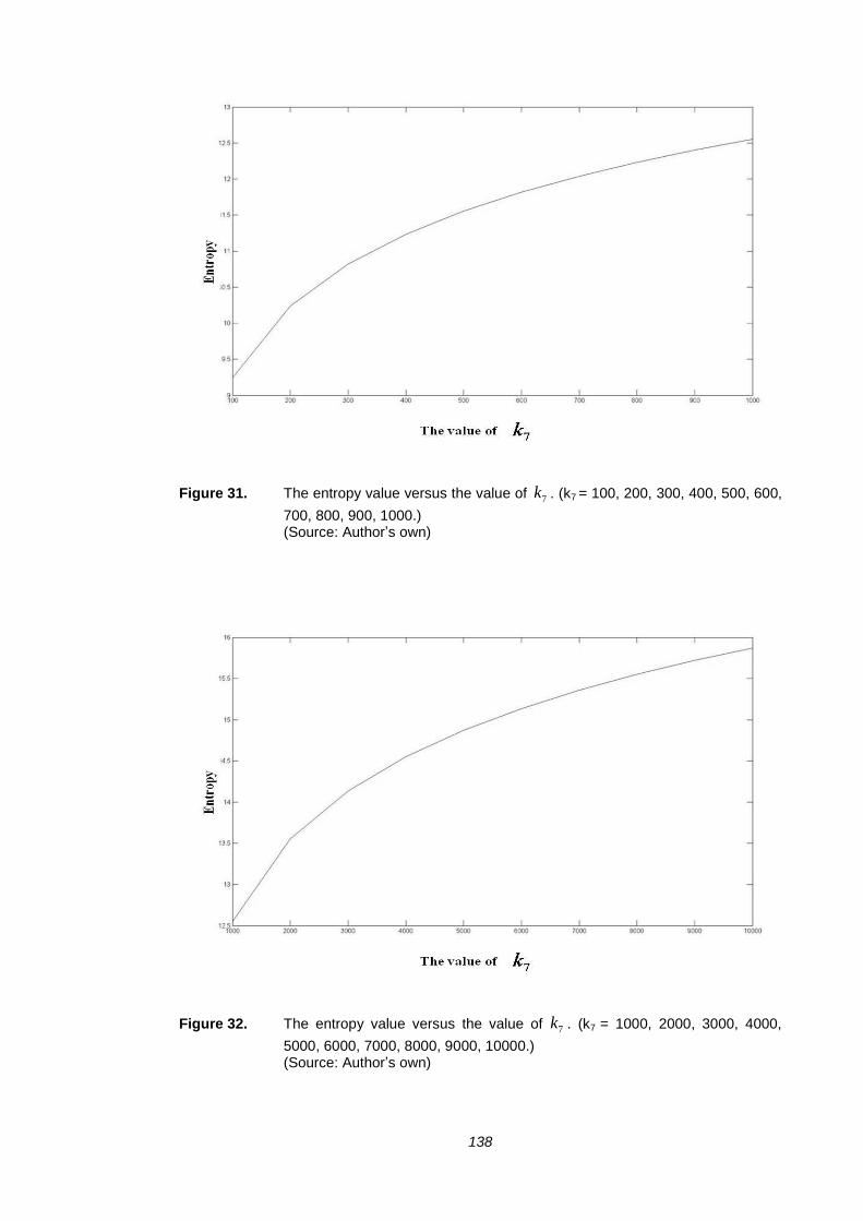
138

Figure 31. The entropy value versus the value of 7k . (k7 = 100, 200, 300, 400, 500, 600,

700, 800, 900, 1000.) (Source: Author’s own)

Figure 32. The entropy value versus the value of 7k . (k7 = 1000, 2000, 3000, 4000,

5000, 6000, 7000, 8000, 9000, 10000.) (Source: Author’s own)

139

Figure 33. The entropy value versus the value of k7. (Source: Author’s own)

Figures 30, 31 and 32 plot the entropy values versus the values of 7k . Figure 33

further summarizes entropy values as 7k increases from 10 to 10000. The level of

increase in entropy decreases when 7k increases. An interesting observation made

from Figures 30, 31 and 32 is that, although the scales of 7k are different in these

three graphs, the three curves show a similar trend.

This subsection has discussed the levels of privacy provided by DOP and STCP. In

DOP, for each dataset X , the level of privacy can be managed by adding a different

number of noise data items. The more noise data items are added, the higher the level

of privacy that can be afforded. A higher level of noise data will undoubtedly lead to

more computational overhead. However, our investigation here has also provided

some insight into the relationship between the effectiveness of the privacy-preserving

capability of the protocol and the number of noise data items used. In cases where the

computation power and computational overhead are of major concern, our protocol

also provides functionality for choosing an affordable number for noise data addition.

An optimal number of noise data items can be determined by evaluating the

increments in entropy versus the number of noise data items used.

140

The privacy level provided by STCP is dependent on the security parameter 5k . This

is because

33 5 nk

l and each 5k is randomly drawn from a uniform distribution

)100,1(U . (Please refer to Figure 22.) The level of 5k can be controlled by managing

the width of the uniform distribution, for example, to use )50,1(U will lead to lower

5k diversity than to use )100,1(U . The larger the value of 5k , the higher the privacy

level that can be achieved by STCP. This property provides an option for choosing an

affordable 5k , which can also be found in DOP. The privacy level provided by DOP

is dependent on the security parameter 4k , since nkn 4' and each 4k is also

randomly drawn from )100,1(U . (Please refer to Figure 21.)

5.4.3.3 Computational Overhead

In a P22NSTP protocol suite execution, 29)'(6)1)(2)(3(2 lnnlll

computational operations are performed, including 20)'(5 nn data perturbation

operations and 9')1)(2)(3(2 lnnlll algebraic operations. (e.g. mapping

table generation, index generation and sign test computation.) The computation cost is

dependent on three factors: the data size n , Alice’s security parameter 'n and Bob’s

security parameter l .

According to our protocol design, 'n and l are both much larger than n .

Consequently, a large n will lead to a great value of 'n and l , respectively. Owing to

this fact, the simulation results can only be acquired when sample size N =10, 20 and

30. Our program can not execute simulation when N≧40 as the data size exceeds the

maximum number of elements in a real double array, i.e. 14108.2 . The number of

computational operations is calculated by averaging the experimental results from

executing the program 100 times.

Figure 34 shows the relationship between the number of computational operations

versus the number of noise data items added by Alice and Bob, respectively, where

the sample size N =10, 20, and 30. The number of computational operations increases

exponentially when 'n and l increase. The more the sample size, the faster the rate of

increase of the number of computational operations.

141

Figure 34. Number of computational operations vs. number of noise data items added by Alice and Bob. (Sample size N = 10, 20, 30.) (Source: Author’s own)

5.4.3.4 Communication Overhead

In total, four messages are generated and transmitted during the protocol suite

execution. Two messages are transmitted by Alice and the other two are by Bob,

respectively. Assuming that I is the number of bits used to represent the value of

each of the plain text data items (e.g. input/output data items), it can be calculated that

the total communication overhead for a P22NSTP protocol suite execution is

Illllnnnn )1)1)(2)(3()3)('()'(2( 22 , where n is the size of both datasets

X and Y , 'n is the security parameter managed by Alice and l is the security

parameter managed by Bob.

Figure 35 shows the relationship between the communication overhead versus the

number of noise data items added by Alice and Bob, respectively, where the sample

size N =10, 20, and 30. The communication overhead is calculated by averaging the

experimental results from executing the program 100 times. The communication

overhead increases approximately linearly when 'n and l increase. The bigger the

sample size, the faster the rate of increase of the communication overhead.

142

Figure 35. Total communication overhead vs. number of noise data items added by Alice and Bob. (Sample size N = 10, 20, 30.) (Source: Author’s own)

5.4.3.5 Protocol Suite Execution Time

As data randomization technique is used in the design of the P22NSTP protocol suite,

the 'n and l generated by each single run of simulation will be different. As a result,

the execution time is calculated by averaging the experimental results from executing

the program 100 times.

Figure 36 shows the relationship between the execution time versus the number of

noise data items added by Alice and Bob, respectively, where the sample size N =10,

20, and 30. The execution time is calculated by averaging the experimental results

from executing the program 100 times. The execution time increases exponentially

when 'n and l increase. The bigger the sample size, the faster the rate of increase of

the execution time.

143

Figure 36. Protocol suite execution time vs. number of noise data items added by Alice and Bob. (Sample size N = 10, 20, 30.) (Source: Author’s own)

5.5 Chapter Summary

This chapter has presented the detailed design of the P22NSTP protocol suite. By

specifically designing the local computational tasks and making use of the data

perturbation techniques, the two parties can perform the sign test computation

securely. The privacy-preserving features of the protocol suite have been analysed

based on protocol components. The correctness, the level of privacy provided, the

computational cost, the communication cost and the execution time have also been

theoretically and experimentally analysed. A comparison of TTP-NST, the P22NSTP

and the P22NSTC will be presented in chapter 7.

144

Chapter 6 A Novel Privacy-preserving Two-party

Nonparametric Sign Test Protocol Suite

Using Cryptographic Primitives (P22NSTC)


This chapter details the design of the P22NSTC protocol suite. Based on this design,

the security threats against privacy requirements are analysed. The correctness, the

level of privacy it provides, the computational overhead and communication overhead

are also theoretically analysed in this chapter. The overview of the P22NSTC protocol

suite is described in section 6.2. Section 6.3 presents the detailed design, including

computation participants, message objects, components of the P22NSTC protocol suite

and elements of the computation. Finally, section 6.4 describes the operation of this

protocol and discusses the correctness, its privacy performance, computational

overhead and communication overhead.

6.2 Overview of the P22NSTC Protocol Suite

This protocol suite is designed for two parties, Alice and Bob, to collaboratively

perform the sign test computation with the assistance from an on-line STTP while

preserving the individual data confidentiality, individual privacy and corporate

privacy of X and Y , where }...,,{ 1 nxxX , }...,,{ 1 nyyY and X and Y are

vertically partitioned. An on-line semi-trusted third party (STTP) is employed in the

design of this protocol suite. Based on the design requirements specified in chapter 3,

the P22NSTC computation is divided into ten local computation tasks. This protocol

suite incorporates two novel protocols that are designed based on data randomization,

data swapping and data transformation techniques. They are data separation protocol

(DSP) and data randomization protocol (DRP). DSP enables the STTP to randomly

split a dataset into two datasets. DRP enables the STTP to generate a randomised

dataset based on a dataset. An additively homomorphic cryptosystem is also used to

support the secure computation of the P22NSTC. On the one hand, the additively

homomorphic cryptosystem is used by both Alice and Bob to encrypt their datasets

before sending them to the STTP. On the other hand, DSP and DRP are used by the

145

STTP to disguise the intermediate computational results before sending them to Alice

and Bob, respectively. The STTP performs computations on both encrypted and

disguised data. The intermediate computational results generated by the

computational tasks are either sent to the other party or kept for the next local

computation. Eight messages are transmitted between the parties and the STTP

throughout the entire computation process.

Before the protocol execution, Alice and Bob first negotiate an additively

homomorphic cryptosystem, i.e. ))(),(,,( skpk DEskpk , where pk is the public key,

sk is the private key, )(pkE is the encryption algorithm and )(skD is the decryption

algorithm. A data transformation function, )(dO , is also negotiated, where

0,1

0,0

0,1

)(

d

d

d

dO .

Local Computational Task 1

Alice encrypts X and generates 1)}({ i

nipk xE .


Bob encrypts Y and generates 1)}({ i

nipk yE .


After receiving 1)}({ i

nipk xE and 1)}({ i

nipk yE , the STTP first computes

)()()( iipkipkipki yxEyExEe , for ni ...,,1 . Assuming that },...,{ 1 neeG , the

STTP then executes DSP using G as data input, and generates 1G and 2G , where 1G

and 2G are two vector datasets, 1G has 1n data items, 2G has 2n data items and

21 nnn . Here we further assume that }...,,{ 11

11 1neeG and }...,,{ 22

12 2neeG .


Using 1G as the data input, the STTP executes DRP and generates 1

1"GT

G , where 1GT

is a permutation matrix of dimension )'()'( 1111 nnnn that is used to distort the

146

order of the data items in 1

1"GT

G . Again, using 2G as the data input, the STTP

executes DRP and generates 2

2" GTG , where

2GT is a permutation matrix of dimension

)'()'( 2222 nnnn that is used to distort the order of the data items in 2

1"GT

G . DRP

not only adds 1'n noise data items into 1G , but also swaps the data item order of the

resulting data vector; also, DRP adds 2'n noise data items into 2G , and swaps the data

item order of the resulting data vector. 1

1"GT

G and 2

2" GTG are two vector datasets of

dimension )'(1 11 nn and )'(1 22 nn , respectively. Here we assume that

}"...,,"{" 1

)'(

1

11 11

1

nn

TeeG G

and }"...,,"{" 2

)'(

2

12 22

1

nn

TeeG G

. The STTP then sends 1

1"GT

G

to Alice and 2

2" GTG to Bob.


After receiving 1

1"GT

G from the STTP, Alice uses )(skD to decrypt every data item in

the dataset. 1

)'(

1

11}"{

i

nnide is then generated where 1"ide is the decryption result of the

thi data item of 1

1"GT

G , for )'(...,,1 11 nni .


By using )(dO , Alice transforms 1

)'(

1

11}"{

i

nnide into 1

)'(

1

11}{

i

nnio . 1

io is an integer value,

for )'(...,,1 11 nni . According to the transformation function, 1

io is either 1, 0 or -1.

Alice then sends 1

)'(

1

11}"{

i

nnide to the STTP.


After receiving 2

2" GTG from the STTP, Bob uses )(skD to decrypt every data item in

the dataset. 1

)'(

2

22}"{

j

nnjde is then generated where 2" jde is the decryption result of the

thj data item of 2

2" GTG , for )'(...,,1 22 nnj .

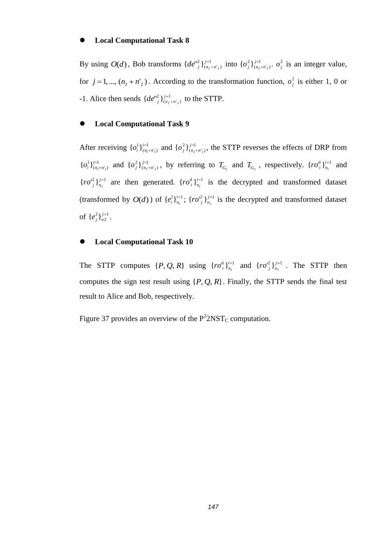
147


By using )(dO , Bob transforms 1

)'(

2

22}"{

j

nnjde into 1

)'(

2

22}{

j

nnjo . 2

jo is an integer value,

for )'(...,,1 22 nnj . According to the transformation function, 2

jo is either 1, 0 or

-1. Alice then sends 1

)'(

2

22}"{

j

nnjde to the STTP.


After receiving 1

)'(

1

11}{

i

nnio and 1

)'(

2

22}{

j

nnjo , the STTP reverses the effects of DRP from

1

)'(

1

11}{

i

nnio and 1

)'(

2

22}{

j

nnjo , by referring to 1GT and

2GT , respectively. 11

1}'{ i

niro and

12

2}'{ j

njro are then generated. 11

1}'{ i

niro is the decrypted and transformed dataset

(transformed by )(dO ) of 11

1}{ i

nie ; 12

2}'{ j

njro is the decrypted and transformed dataset

of 1

2

2}{ j

nje .


The STTP computes },,{ RQP using 11

1}'{ i

niro and 12

2}'{ j

njro . The STTP then

computes the sign test result using },,{ RQP . Finally, the STTP sends the final test

result to Alice and Bob, respectively.

Figure 37 provides an overview of the P22NSTC computation.

148

Figure 37. An overview of the P22NSTC computation.


6.3 The Design in Detail

6.3.1 Computation Participants and Message Objects

Computation Participants:

The protocol is designed for two parties, Alice and Bob, who hold dataset X and Y

respectively, where }...,,{ 1 nxxX , }...,,{ 1 nyyY and X and Y are vertically

partitioned. An on-line STTP is also used in the protocol suite. The two parties

interact with the STTP to carry out the P22NSTC computation.

149

Message Objects:

Eight messages are transmitted during the entire protocol suite execution:

Message 1: Alice sends the encryption result, i.e. 1)}({ i

nipk xE , and z to the STTP.

That is, },,)}({{ 1

1 zxEmsg i

nipk .

)( ipk xE is a ciphertext. There are )2( n data items in 1msg .

Message 2: Bob sends the encryption result, i.e. 1)}({ i

nipk yE , and z to the STTP.

That is, },,)}({{ 1

2 zyEmsg i

nipk .

)( jpk xE is a ciphertext. There are )2( n data items in 2msg .

Message 3: The STTP sends 1

1"GT

G to Alice. That is, }"{ 1

13GT

Gmsg .

Assuming that }"...,,"{" 1

)'(

1

11 11

1

nn

TeeG G

, there are )'( 11 nn data items

in 3msg .

Message 4: The STTP sends 2

2" GTG to Bob. That is, }"{ 2

24GT

Gmsg .

Assuming that }"...,,"{" 2

)'(

2

12 22

1

nn

TeeG G

, there are )'( 22 nn data

items in 4msg .

Message 5: Alice sends the decryption result, i.e. 1

)'(

1

11}{

i

nnio , to the STTP. That is,

}}{{ 1

)'(

1

5 11

i

nniomsg .

There are )'( 11 nn data items in 5msg .

Message 6: Bob sends the decryption result, i.e. 1

)'(

2

22}{

j

nnjo , to the STTP. That is,

}}{{ 1

)'(

2

6 22

j

nnjomsg .

There are )'( 22 nn data items in 6msg .

150

Message 7: The STTP sends the final test result, i.e. FR , to Alice. That is,

}{7 FRmsg .

There is only one integer value data item in 7msg .

Message 8: The STTP sends the final test result, i.e. FR , to Bob. That is,

}{8 FRmsg .

There is only one integer value data item in 8msg .

6.3.2 Components of the P22NSTC Protocol Suite

The P22NSTc protocol suite consists of three components, they are (1) the additively

homomorphic cryptosystem, (2) the data separation protocol (DSP) and (3) the data

randomization protocol (DRP). The three components are detailed in the following

subsections.

6.3.2.1 Additively Homomorphic Encryption Scheme

An additively homomorphic cryptosystem, i.e. ))(),(,,( skpk DEskpk , is negotiated

by Alice and Bob before the P22NSTC protocol suite execution. It has the property of

)()()( yxEyExE pkpkpk and yxyxED pksk ))(( . It is used by both Alice and

Bob to respectively encrypt X and Y before sending it to the STTP. This prevents

the individual data confidentiality and individual privacy of the joint dataset from

being disclosed to the STTP. Simultaneously, the STTP can still perform a

multiplication operation on the encrypted data items.

6.3.2.2 Data Separation Protocol (DSP)

The data separation protocol (DSP) is designed to enable the STTP to randomly

separate a dataset G into 1G and 2G . Assuming that }...,,{ 1 nddG ,

}...,,{ 11

11 1nddG and }...,,{ 22

12 2nddG , where 21 nnn . The detail of DSP is

described below.

151

Data Separation Protocol (DSP)

Input: G .

Output: 1G and 2G .

(1) STTP randomly selects an integer 1n from ]3

2...,,

3[

nn, with a probability of

)33

2(

1

nn.

(2) STTP computes 12 nnn .

(3) STTP randomly separates G into two subsets, 1G and 2G , where 1G has 1n

data items, 2G has 2n data items, i

jd equals some kd for }...,,1{ nk ,

}2,1{i , and 11 |}...,,1{ inj or 22 |}...,,1{ inj .

Figure 38. The DSP algorithm. (Source: Author’s own)

Here 1G has 1n data items, 2G has 2n data items and 21 nnn . As 1n is chosen

from n...,,1 , 1n may be very small or close to 1 (this leads to a very large 2n ), or its

value is large leading to a very smaller 2n . To avoid such extreme cases, DSP is

designed to select 1n from ]3

2...,,

3[

nn.

6.3.2.3 Data Randomization Protocol (DRP)

The data randomization protocol (DSP) is designed to enable the STTP to randomly

generate a randomised dataset GTG" based on a dataset G . Assuming that

}...,,{ 1 nddG , the STTP first generates a noise dataset }'...,,'{' '1 nddG , where

)1('2

2

nnnn

. The STTP then merges G and 'G . Assuming that

}'...,,',...,,{" '11 nn ddddG , the STTP finally generates GTG" by swapping the order

of "G . The detail of DRP is described below.

152

Data Randomization Protocol (DRP)

Input: G .

Output: GTG'

(1) STTP randomly selects an integer 'n from )]1(,...,2

[2

nn

n.

(2) For '...,,1 ni , STTP randomly chooses it and iu from }...,,1{ n , i.e. the STTP

has )},(...,),,{( ''11 nn utut .

(3) For ',...,1 ni , STTP generates ii uti ddd ' , i.e. STTP has }'...,,'{ '1 ndd . We

further assume that }'...,,'{' '1 nddG .

(4) STTP generates "G by merging G and 'G such that

}'...,,',...,,{" '11 nn ddddG .

(5) STTP generates a permutation matrix GT of dimension )'()'( nnnn .

(6) STTP generates GTG" by computing G

TTGG G "" .

Figure 39. The DRP algorithm. (Source: Author’s own)

The rationales of key computation steps in Figure 39 are further described below.

The purpose of DRP is to enable the STTP to generate the randomised dataset

GTG' based on a dataset G . DOP will be used by the STTP to generate a

randomised dataset base on a ciphertext dataset in the P22NSTC suite execution.

For this reason, the noise data items should also have the same property of

ciphertexts that are encrypted by the same cryptosystem. The noise data items

are generated by multiplicating two of the data items in G , i.e. ii uti ddd ' .

Thus id ' has the same property as it

d and iud .

To ensure that sufficient noise data items are supplied, 'n is designed to be

randomly selected from )]1(...,,2

[2

nn

n. Thus 'n can be guaranteed to be at

least

2

n times more than n . This interval is configurable. By controlling the

length of this interval, a required level of security can be achieved.

153

How 1G and 2G are generated from G .

How 1G and 2G are generated plays a pivotal role in the computation, as they are

used as the input in DSP to generate GTG" . There are two design issues associated

with this generation. The first issue is how to generate a sufficient number of random

noise data items and how to avoid the extreme cases where 1n or 2n is close to n . In

such cases, the number of noise data items that can be generated by DSP will be

extremely limited. Our solution to resolve this problem is to set 1n and 2n to a value

close to

2

n, i.e. to let

3

2

3

nn

ni , }2,1{i . In this way the size of the noise

data items pool can be larger than ))13

(3

(

nn and smaller than

))13

2(

3

2(

nn. Secondly, the number of random numbers that can be generated

for 1

1"GT

G and 2

2" GTG are less than )1( 11 nn and )1( 22 nn , respectively. One way to

address this problem is to generate new random inputs using more than three data

inputs in 1G or 2G in step (2) and step (3). For example, the STTP can initially

randomly select a number, mn , from 1n or 2n , then randomly pick up mn data items

from 1G or 2G and finally generate the new noise data item by multiplying these mn

data items. In the case where

221

nnn , we may increase the size of the selection

pool of 1

1"GT

G and 2

2" GTG from

2

2

n

C to

2

12

2

3

2

2 ...

n

n

nn

CCC .

How Privacy is preserved.

Upon a protocol suite execution, the probability for a curious party to successfully

guess the value of 1n and 1'n (or 2n and 2'n ) from 1

1"GT

G (or 2

2" GTG ) is

)2'(

1

11 nn

(or )2'(

1

22 nn). In the case where a party has successfully inferred 1n and 1'n (or

2n and 2'n ), it has to further infer 1GT (or 2GT ) in order to work out the inputs in 1G

(or 2G ), thus disclosing G . In such case, the probability of disclosing the data inputs

154

of 1G (or 2G ) is )2'()!'(

)!'()!(

1111

11

nnnn

nn (or

)2'()!'(

)!'()!(

2222

22

nnnn

nn), which is

negligible.

6.4 The P22NSTC Protocol Suite and Its Operation

The goal of the P22NSTC protocol is to compute the test result of a sign test

computation on X and Y with the assistance from an on-line STTP, while keeping

Alice from knowing Y and },,{ RQP , keeping Bob from knowing X and },,{ RQP ,

and keeping the STTP from knowing X and Y . Prior to executing the computation,

Alice and Bob are assumed to have negotiated , z and the use of an additively

homomorphic cryptosystem with a key pair ),( skpk , i.e. ))(),(,,( skpk DEskpk . They

have also jointly defined a function )(dO , where

0,1

0,0

0,1

)(

d

d

d

dO . Using the

building blocks described in chapter 4 and the components described in section 6.3.2,

we can now design the P22NSTC protocol.

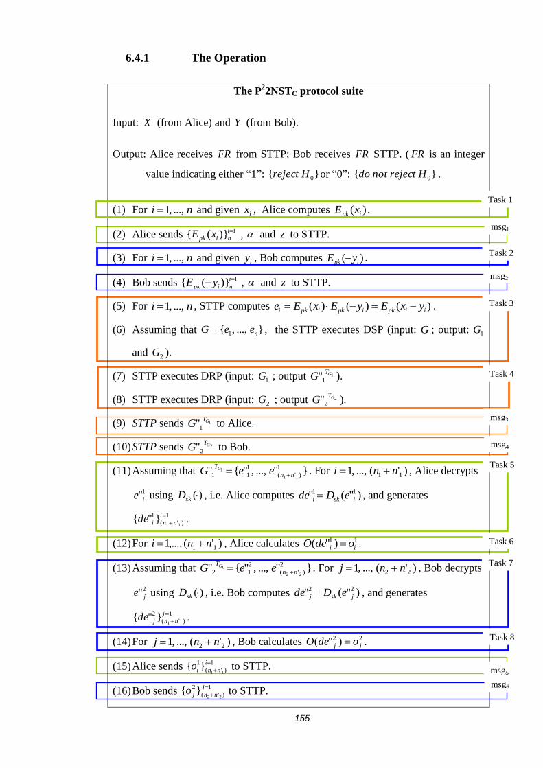
155

6.4.1 The Operation

The P22NSTC protocol suite

Input: X (from Alice) and Y (from Bob).

Output: Alice receives FR from STTP; Bob receives FR STTP. ( FR is an integer

value indicating either “1”: }{ 0Hreject or “0”: }{ 0Hrejectnotdo .

(1) For ni ...,,1 and given ix , Alice computes )( ipk xE .

(2) Alice sends 1)}({ i

nipk xE , and z to STTP.

(3) For ni ...,,1 and given iy , Bob computes )( ipk yE .

(4) Bob sends 1)}({ i

nipk yE , and z to STTP.

(5) For ni ...,,1 , STTP computes )()()( iipkipkipki yxEyExEe .

(6) Assuming that }...,,{ 1 neeG , the STTP executes DSP (input: G ; output: 1G

and 2G ).

(7) STTP executes DRP (input: 1G ; output 1

1"GT

G ).

(8) STTP executes DRP (input: 2G ; output 2

2" GTG ).

(9) STTP sends 1

1"GT

G to Alice.

(10) STTP sends 2

2" GTG to Bob.

(11) Assuming that }"...,,"{" 1

)'(

1

11 11

1

nn

TeeG G

. For )'(...,,1 11 nni , Alice decrypts

1"ie using )(skD , i.e. Alice computes )"(" 11

iski eDde , and generates

1

)'(

1

11}"{

i

nnide .

(12) For )'(,...,1 11 nni , Alice calculates 11 )"( ii odeO .

(13) Assuming that }"...,,"{" 2

)'(

2

12 22

1

nn

TeeG G

. For )'(...,,1 22 nnj , Bob decrypts

2" je using )(skD , i.e. Bob computes )"(" 22

jskj eDde , and generates

1

)'(

2

11}"{

j

nnjde .

(14) For )'(...,,1 22 nnj , Bob calculates 22 )"( jj odeO .

(15) Alice sends 1

)'(

1

11}{

i

nnio to STTP.

(16) Bob sends 1

)'(

2

22}{

j

nnjo to STTP.

Task 1

Task 2

Task 3

Task 4

Task 5

Task 6

Task 8

Task 7

msg1

msg2

msg3

msg4

msg5

msg6

156

(17) Let }'...,,'{' 1

)'(

1

1

1

11 nnooO , STTP computes T

GG TOO11

11 '' .

(18) Let }'...,,'{' 1

)'(

1

1

1

111 nnG roroO , STTP singles out }'...,,'{ 11

1 1nroro from

}'...,,'{' 1

)'(

1

1

1

111 nnG roroO , where }'...,,'{ 11

1 1nroro contains the first 1n data items

in }'...,,'{' 1

)'(

1

1

1

111 nnG roroO .

(19) Let }'...,,'{' 2

)'(

2

1

2

22 nnooO , STTP computes T

GG TOO22

22 '' .

(20) Let }'...,,'{' 2

)'(

2

1

2

222 nnG roroO , STTP singles out }'...,,'{ 22

1 2nroro from

}'...,,'{' 2

)'(

2

1

2

222 nnG roroO , where }'...,,'{ 22

1 2nroro contains the first 2n data

items in }'...,,'{' 2

)'(

2

1

2

222 nnG roroO .

(21) STTP computes P by calculating the frequency of 1 in 11

1}'{ i

niro and 12

2}'{ j

njro .

(22) STTP computes Q by calculating the frequency of 0 in 11

1}'{ i

niro and 12

2}'{ j

njro .

(23) STTP computes R by calculating the frequency of -1 in 11

1}'{ i

niro and 12

2}'{ j

njro .

(24) STTP performs the sign test by using RQPzn ,,,,, and generates the final test

result FR .

(25) STTP sends FR to Alice

(26) STTP sends FR to Bob.

Figure 40. The P22NSTC algorithm.



elements in Figure 40 are further described below.

In step (5), ie is a ciphertext generated by computing )()( ipkipk yExE , where

)( ipk xE and )( ipk yE are two ciphertexts encrypted by the additively

homomorphic cryptosystem ))(),(,,( skpk DEskpk , for ni ...,,1 .

In step (6), assuming that }...,,{ 1 neeG , 1G and 2G are generated by DSP where

21 GGG and 21 GG . We further assume }...,,{ 11

11 1neeG and

}...,,{ 22

12 2neeG , where 21 nnn , i

je equals some ke for }...,,1{ nk , }2,1{i ,

and 11 |}...,,1{ inj or 22 |}...,,1{ inj .

In steps (7) and (9), }"...,,"{" 1

)'(

1

11 11

1

nn

TeeG G

.

Task 10

msg8

msg7

Task 9

157

In steps (8) and (10), }"...,,"{" 2

)'(

2

12 22

1

nn

TeeG G

.

In step (11), for )'(...,,1 11 nni , 1"ide is a plaintext.

In step (12), Alice uses the transformation function, i.e. )(dO , to transform 1"ide

into 1

io . The value of 1

io is either 1, 0 or -1.

In step (13), for )'(...,,1 22 nnj , 2" jde is a plaintext.

In step (14), Bob uses the transformation function, i.e. )(dO , to transform 2" jde

into 2

jo . The value of 2

jo is either 1, 0 or -1.

In steps (17) - (18), assuming that 1'O is a row vector of dimension )'(1 11 nn

where the row order has been swapped. Then 1

1'GO is a row vector of dimension

)'(1 11 nn where the row order has been restored, i.e. 11 1

11

1 ]'...,,'[ nnroro is the

key vector (the decrypted and transformed computational result of 1G ) and

1111 '1

1

)'(

1

)1( ]'...,,'[ nnnn roro is the noise vector.

In steps (19) - (20), assuming that 2'O is a row vector of dimension )'(1 22 nn

where the row order has been swapped. Then 2

2'GO is a row vector of dimension

)'(1 22 nn where the row order has been restored, i.e. 22 1

22

1 ]'...,,'[ nnroro is the

key vector (the decrypted and transformed computational result of 2G ) and

2222 '1

2

)'(

2

)1( ]'...,,'[ nnnn roro is the noise vector.

How privacy-preservation is achieved.

Because ix and iy are encrypted before being sent to the STTP and the STTP does

not have access to the encryption key pair ),( skpk , X and Y are kept private from

the STTP. For operations performed by Alice (or by Bob), 1

1"GT

G (or 2

2" GTG ) only

contains 1n (or 2n ) data items from G with the rest, i.e. 1'n (or 2'n ), being noise data

items, and )',( 11 nn (or )',( 22 nn ) being only known to the STTP. As shown in

subsection 6.3.2.3, the chance of Alice (or Bob) to guess G from 1

1"GT

G (or G from

2

2" GTG ) is negligible. The only possible inference for Alice (or for Bob) to make is to

guess a subset of G . In Alice’s case (for Bob’s case, the discussion is identical except

that 1

1"GT

G is replaced by 2

2" GTG ), for example, there are 1

33

2

nn possibilities

158

regarding the possible data item subsets of G , i.e. 1

1"GT

G contains

3

ndata items

from G , 1

1"GT

G contains 13

n data items from G ,…, 1

1"GT

G contains

3

2n data

item from G . The probability for Alice to successfully guess these data item subsets

is

))133

2()!'()'((

)!)!'(

Pr

1111

3

2

3

11

nnnnnn

iinni

n

ni

AG . The upper bound of AGPr is

)!'()'(

)!3

2)

3

2'(

3

2(

Pr1111

11

nnnn

nnnn

n

up

AG

, while the lower bound of AGPr is

)!'()'(

)!3

)3

'(3

(

Pr1111

11

nnnn

nnnn

n

lowAG

, i.e. up

AGAGlowAG PrPrPr . And so does BGPr ,

i.e. up

BGBGlowBG PrPrPr .

In a case when malicious Alice (or Bob) sends fake X (or Y ) to the STTP, the most

optimistic inference she (or he) can get from 1

1"GT

G (or 2

2" GTG ) is partial information

of G , with probability up

AGPr (or up

BGPr ). If malicious Alice (or Bob) further decides

to send fake 1

)'(

1

11}{

i

nnio (or 1

)'(

2

22}{

j

nnjo ) to the STTP, she (or he) can only break this

computation, no further information will be gained.

6.4.2 Correctness

In steps (7) and (8) of Figure 40, the STTP has employed DRP to transform 1G and

2G into 1

1"GT

G and 1

1"GT

G , respectively. In steps (12) and (14), Alice and Bob further

transform 1"ide and 2" jde using

0,1

0,0

0,1

)(

d

d

d

dO , respectively. By reversing the

effects of 1T and 2T , 1

1'GO and

1

2'GO can be restored. As }'...,,'{' 1

)'(

1

1

1

111 nnG roroO and

}'...,,'{' 2

)'(

2

1

2

222 nnG roroO , }'...,,'{ 11

1 1nroro and }'...,,'{ 22

1 2nroro can then be identified.

}'...,,'{ 11

1 1nroro is the transformed comparison results of )( ii yx , for 1...,,1 ni ;

159

}'...,,'{ 22

1 2nroro is the transformed comparison results of )( ii yx , for nni ...,,11 ,

where 21 nnn . The transformed result of YX can be acquired. The STTP can

then use this to compute P , Q and R . Therefore the sign test result can be

computed correctly.

6.4.3 Protocol Analysis

6.4.3.1 Privacy Analysis against Privacy Requirements

The privacy-preserving properties provided by the P22NSTC protocol suite can be

classified as threefold:

(1) The privacy protection provided by the additively homomorphic cryptosystem. The

cryptosystem is used by both Alice and Bob to secure their respective dataset prior

to sending to the STTP. It protects the individual data confidentiality and

individual privacy of X and Y from being known to the STTP. The Paillier

cryptosystem is used in the design of the P22NSTC protocol suite. As the Paillier

cryptosystem has been proven to be secure in the literature [PAIL’99b], here it is

regarded as being irreversible, i.e. an intruder can not decrypt the encrypted data

items.

(2) The privacy protection provided by the DSP and the DRP. The use of DSP and

DRP prevents individual data confidentiality and individual privacy of Y from

being known to Alice, individual data confidentiality and individual privacy of X

from being known to Bob and corporate privacy of },,{ RQP from being known

to Alice and Bob. As the two protocols are designed based on data disguising

techniques, the level of privacy provided is dependent on 1n , 1'n , 2n and 2'n .

(3) The privacy protection provided by the many-to-one transformation function. This

function is used by both Alice and Bob to secure the values of the differences of

the pairwised comparisons. This function is irreversible. Even if the STTP

receives the plain transformation results, it can not infer the actual values of the

difference of the pairwised comparison.

As the additively homomorphic cryptosystem and the data transformation technique

are assumed to preserve privacy completely, in this subsection, we focus on analysing

the level of privacy provided by DSP and DRP. This can be further classified into two

160

aspects: (1) the privacy-preserving effect provided by the DSP and (2) the privacy-

preserving effect provided by the DRP.

6.4.3.2 Quantify Level of Privacy Using Entropy

The case where malicious Alice wants to infer information from 1

1"GT

G is analysed in

this subsection. (The case is identical to malicious Bob’s case.) The probability for

malicious Alice to guess 1n is nnn

3

33

2

1

. The probability for malicious Alice

to guess 1'n is )2(

2

2)1(

1

1

2

1

2

111

nnnnn

and the probability to figure out the

permutation matrix 1GT is

)!'(

1

11 nn . The probability for malicious Alice to infer the

correct ix is ))!')((2(

6)(

111

2

1

)'',,( 1111 nnnnnxP inNnNnN

for 1,...,1 ni and the

probability for malicious Alice to infer the incorrect ix (noise data item) is

1

1111

2

1)'',,(

'

))!')((2(

61

)(

1

1111 n

nnnnnxP

n

i

inNnNnN

for )'(...,),1( 111 nnni ,

such that 1)(11

1111

'

1 )'',,(

nn

i inNnNnN xP . Thus, the entropy value of DRP and DSP

is

))'

))!')((2(

61

(log)'

))!')((2(

61

(

)))!')((2(

6(log)

))!')((2(

6((

11

1

11

1

1111

'

11

1111

2

12

1

1111

2

1

111

2

1

21111

2

1

)'',,(

nn

ni

n

i

n

i

n

i

nNnNnN

n

nnnnn

n

nnnnn

nnnnnnnnnn

h

.

n is the size of Alice’s dataset. 1n is a value randomly drawn from ]3

2,

3[

nn and

managed by the STTP. 1'n is a value randomly drawn from )]1(,2

[ 11

2

1

nn

n and also

managed by the STTP.

161

The analysis of entropy values will be performed by assuming sample size N = {10,

20, 30, 40, 50, 60, 70, 80, 90, 100, 200, 300, 400, 500, 600, 700, 800, 900, 1000, 2000,

3000, 4000, 5000, 6000, 7000, 8000, 9000, 10000, 20000, 30000, 40000, 50000,

60000, 70000, 80000, 90000, 100000}. According to our protocol design, 1n (or 2n )

and 1'n (or 2'n ) are both larger than n . Consequently, a large n will lead to a large

number of 1n (or 2n ) and 1'n (or 2'n ), respectively. In addition, the computation of

entropy involves the factorial computation of )!'( 11 nn and the logarithm

computation of )))!')((2(

6(log

111

2

1

2nnnnn

. The value of

)))!')((2(

6(log

111

2

1

2nnnnn

can not be calculated by MATLAB when N≧30 as

0))!')((2(

6

111

2

1

nnnnn

, MATLAB returns the value as a NaN (Not-a-Number).

As our purpose is to analyse the trend of the entropy value curve and the value of

))!')((2(

6

111

2

1 nnnnn decreases when sample size increases, we use the value of

))!')((2(

6

111

2

1 nnnnn generated from N=20 in the cases of N≧30. Since 1n , 2n , 1'n

and 2'n are generated randomly, the entropy values are calculated by averaging the

experimental results from executing the program 100 times.

Tables 13-16 show the entropy values and the increment of entropy when sample size

changes. Figures 41-44 plot the relationship between the entropy values and sample

sizes. Figure 45 further summarized the overview of the entropy versus sample size. It

can be observed from Figures 41-44 that although the scales of sample size of these

four figures are different, they all show a similar trend. The level of increase in

entropy decreases when sample size increases. The highest level of increase of

entropy can be observed when sample size is under 100. When the sample size

exceeds 10000, the level of increase in entropy is more gradual than the cases where

sample sizes are smaller then 10000.

162

Table 13. The entropy value and the increment versus sample size. (Sample size N = 10, 20, 30, 40, 50, 60, 70, 80, 90, 100.) (Source: Author’s own)




163

Figure 41. The entropy value versus sample size. (Sample size N = 10, 20, 30, 40, 50, 60, 70, 80, 90, 100.) (Source: Author’s own)


164



165

Figure 45. The entropy value versus sample size. (overview) (Source: Author’s own)

6.4.3.3 Computational Overhead

In this protocol, 19)''(45 21 nnn computations are performed, which includes

)''(3 21 nnn cryptographic computations, )''(26 21 nnn data disguising

computations and )''(13 21 nnn non-privacy-preserving computations

(multiplication, addition and sign test operation). The computation cost increases

along with data size n and security parameters 1'n and 2'n .

Owing to the effect of the data randomization technique in DRP, our program can not

execute simulation when N≧700 as the data size exceeds the maximum number of

elements in a real double array, i.e. 14108.2 . The simulation results are acquired

when sample size N = {10, 20, 30, 40, 50, 60, 70, 80, 90, 100, 200, 300, 400, 500, 600,

700}. A key length of 128 bits is used in the additively homomorphic cryptosystem.

The computational overhead is calculated by averaging the experimental results from

executing the program 100 times.

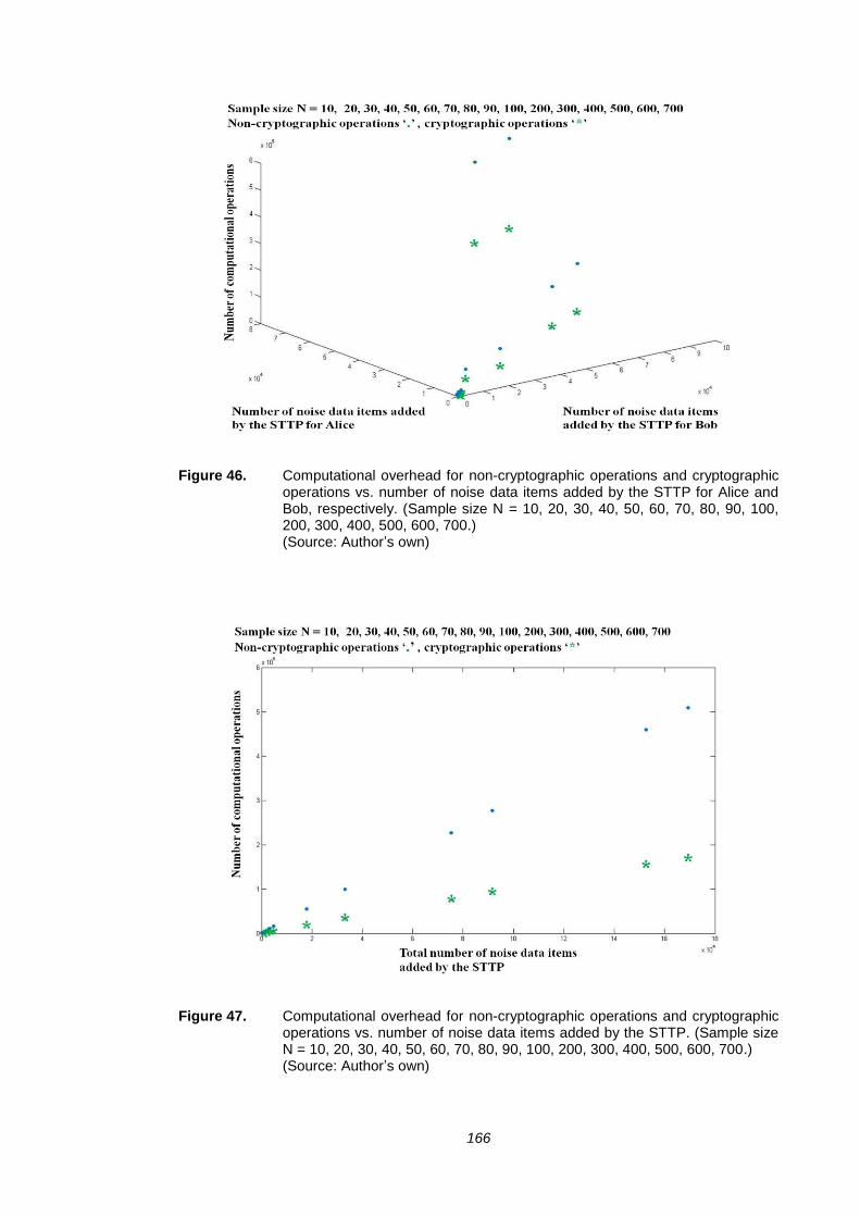
166

Figure 46. Computational overhead for non-cryptographic operations and cryptographic operations vs. number of noise data items added by the STTP for Alice and Bob, respectively. (Sample size N = 10, 20, 30, 40, 50, 60, 70, 80, 90, 100, 200, 300, 400, 500, 600, 700.) (Source: Author’s own)

Figure 47. Computational overhead for non-cryptographic operations and cryptographic operations vs. number of noise data items added by the STTP. (Sample size N = 10, 20, 30, 40, 50, 60, 70, 80, 90, 100, 200, 300, 400, 500, 600, 700.) (Source: Author’s own)

167

Figures 46 and 47 show the relationship between the number of computational

operations versus the number of noise data items added by the STTP for Alice and

Bob, respectively. The number of computational operations increases approximately

linearly when 1'n and 2'n increase. The number of non-cryptographic operations is

larger than the number of cryptographic operations.

6.4.3.4 Communication Overhead

Eight messages are exchanged during the entire protocol suite execution, with four of

them being transmitted by the STTP, and two by Alice and Bob, respectively.

Assuming that I is the number of bits used to represent the value of each of the

plaintext data items (e.g. input/output date items) and 'I is the number of bits needed

to represent the value of each of the ciphertext data items, the communication

overhead for the P22NSTC protocol suite is ')''34()''2( 2121 InnnInnn ,

where n is the size of X and Y and 2211 ',,', nnnn are security parameters randomly

chosen by the STTP.

Figures 48 and 49 show the relationship between the communication overhead versus

the number of noise data items added by the STTP for Alice and Bob, respectively.

The amount of communication overhead is shown in two aspects: the number of non-

encrypted data items and the number of encrypted data items. The communication

overhead is calculated by averaging the experimental results from executing the

program 100 times. The communication overhead increases approximately linearly

when the number of noise data items increases. An observation can be made that the

number of non-encrypted data items and the number of encrypted data items are

similar. This echoes the theoretical result, i.e. ')''34()''2( 2121 InnnInnn .

As 21 '' nnn , this value is largely dependent on 21 '' nn .

168

Figure 48. Communication overhead for non-encrypted data items and encrypted data items vs. number of noise data items added by the STTP for Alice and Bob, respectively. (Sample size N = 10, 20, 30, 40, 50, 60, 70, 80, 90, 100, 200, 300, 400, 500, 600, 700.) (Source: Author’s own)

Figure 49. Communication overhead for non-encrypted data items and encrypted data items vs. number of noise data items added by the STTP. (Sample size N = 10, 20, 30, 40, 50, 60, 70, 80, 90, 100, 200, 300, 400, 500, 600, 700.) (Source: Author’s own)

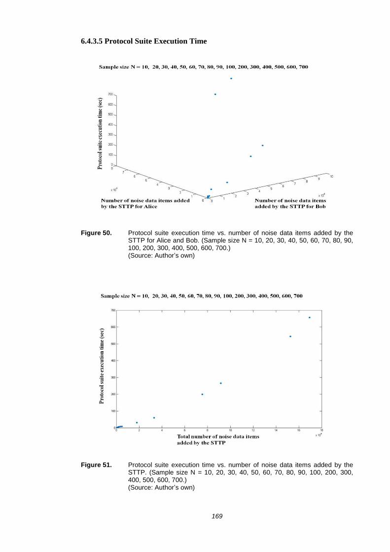
169

6.4.3.5 Protocol Suite Execution Time

Figure 50. Protocol suite execution time vs. number of noise data items added by the STTP for Alice and Bob. (Sample size N = 10, 20, 30, 40, 50, 60, 70, 80, 90, 100, 200, 300, 400, 500, 600, 700.) (Source: Author’s own)

Figure 51. Protocol suite execution time vs. number of noise data items added by the STTP. (Sample size N = 10, 20, 30, 40, 50, 60, 70, 80, 90, 100, 200, 300, 400, 500, 600, 700.) (Source: Author’s own)

170

Figures 50 and 51 show the relationship between the execution time versus the

number of noise data items added by the STTP for Alice and Bob, respectively. The

execution time is calculated by averaging the experimental results from executing the

program 100 times. The execution time increases exponentially when 1'n and 2'n

increase. The more the noise data items, the faster the rate of increase of the execution

time.

6.5 Chapter Summary

This chapter has presented the detailed design of the P22NSTC protocol suite. By

specifically designing the local computational tasks and making use of the data

perturbation techniques and the homomorphic cryptosystem, with the assistance from

the on-line STTP, the two parties can securely perform the sign test computation. The

privacy-preserving features of the protocol suite have been analysed for each

computational task on a task base. With the assistance from the STTP, this protocol

suite can prevent a party from knowing other party’s dataset and the intermediate

computational results of the computation. It also prevents the STTP from knowing the

parties’ private datasets. The correctness, the level of privacy provided, the

computational cost, the communication cost and the execution time have also been

theoretically and experimental analysed. A comparison of the TTP-NST, the P22NSTP

and the P22NSTC will be presented in chapter 7.

171

Chapter 7 A Comparison of the TTP-NST, the P22NSTP

and the P22NSTC


This chapter compares the performances of the P22NSTP and the P

22NSTC against the

TTP-NST. The TTP-NST, the P22NSTP and the P

22NSTC algorithms have all been

prototyped and implemented using MATLAB. As MATLAB provides sign test

computation function in its statistical computation library, the TTP-NST program uses

the provided function to carry out the sign test computation. The P22NSTP protocol

suite is a novel design; its algorithm is completely programmed by MATLAB.

However, since MATLAB does not provide cryptosystem library, the homomorphic

cryptosystem to be used in the novel P22NSTC protocol suite is programmed in JAVA

code as a function. The P22NSTC protocol suite then employs this function during the

protocol suite execution. Section 7.2 presents the comparison of privacy protections

provided by the three algorithms. The comparisons of computational overhead and

communication overhead are presented in section 7.3 and 7.4 respectively. Section 7.5

compares the execution times and finally section 7.6 summarises this chapter.

172

7.2 A Comparison of Privacy Protection

Figure 52. A comparison of privacy protection by the TTP-NST, the P22NSTP and the

P22NSTC.


Figure 52 summarises the privacy protection provided by the TTP-NST and the

designed solutions. It is compared against individual data confidentiality, individual

privacy and corporate privacy, each with three privacy requirements.

In the TTP-NST model, the TTP does all the computation for Alice and Bob. Alice

has no access to Y (i.e. L12 is completely protected.) and Bob has no access to X

(i.e. L11 is completely protected.); after the completion of the computation, all they

know are their own private data input and the final computation result (i.e. L21, L22

L31 and L31 are all completely protected.). In this model, the TTP knows all the

information about X and Y (i.e. L13, L23 and L33 are not protected.), except for the

identities of the data subject in X and Y .

In the P22NSTP computation, no third party is involved (i.e. L13, L23 and L33 are

completely protected.); the computation is carried out by Alice and Bob jointly. It is

noted that Y is completely kept away from Alice (i.e. L12 is completely protected.) as

Alice has no access to Y during the P22NSTP execution. All other privacy protection

requirements, i.e. L11, L21, L22, L31 and L32 are protected by data perturbation

techniques. More specifically, L11 and L21 are protected by DOP; L22 is protected

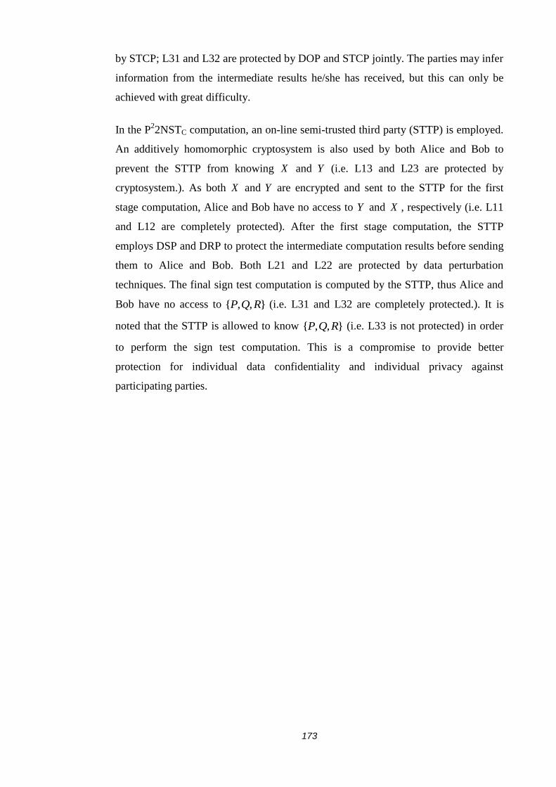
173

by STCP; L31 and L32 are protected by DOP and STCP jointly. The parties may infer

information from the intermediate results he/she has received, but this can only be

achieved with great difficulty.

In the P22NSTC computation, an on-line semi-trusted third party (STTP) is employed.

An additively homomorphic cryptosystem is also used by both Alice and Bob to

prevent the STTP from knowing X and Y (i.e. L13 and L23 are protected by

cryptosystem.). As both X and Y are encrypted and sent to the STTP for the first

stage computation, Alice and Bob have no access to Y and X , respectively (i.e. L11

and L12 are completely protected). After the first stage computation, the STTP

employs DSP and DRP to protect the intermediate computation results before sending

them to Alice and Bob. Both L21 and L22 are protected by data perturbation

techniques. The final sign test computation is computed by the STTP, thus Alice and

Bob have no access to },,{ RQP (i.e. L31 and L32 are completely protected.). It is

noted that the STTP is allowed to know },,{ RQP (i.e. L33 is not protected) in order

to perform the sign test computation. This is a compromise to provide better

protection for individual data confidentiality and individual privacy against

participating parties.

174

7.3 A Comparison of Computational Overhead

Figure 53. A comparison of computation overhead. (Source: Author’s own)

As mentioned in chapter 5 and 6, the total computations needed for the P22NSTP

computation is 29)'(6)1)(2)(3(2 lnnlll of computations, including

20)'(5 nn non-privacy-preserving computations and

9')1)(2)(3(2 lnnlll data disguising computations. The computational

complexity of the P22NSTP is )( 3nO . The total computations needed for the P

22NSTC

is 19)''(45 21 nnn . This includes )''(3 21 nnn cryptographic computations,

)''(26 21 nnn data disguising computations and )''(13 21 nnn non-privacy-

preserving computations (multiplication, addition and sign test operation). The

computational complexity of the P22NSTP is )(nO . )4( n non-privacy-preserving

computations are performed in the TTP-NST. The computation complexity of TTP-

NST is )(nO . It can be seen from Figure 53 that the computation complexity of the

P22NSTC is smaller than the P

22NSTP. This is because of the noise data item generated

in the P22NSTP.

175

7.4 A Comparison of Communication Overhead

Figure 54. A comparison of communication overhead (Source: Author’s own)

Both the TTP-NST and the P22NSTP use four messages throughout the computation,

while the P22NSTC use eight messages. The extra four messages are used for Alice and

Bob to interact with the STTP. Assuming that I is the number of bits used to represent

the value of each of the plaintext data items (e.g. input/output date items) and 'I is the

number of bits needed to represent the value of each of the cipher text data items, the

TTP-NST consumes nI4 bits communication costs and the P22NSTP consumes

Illllnnnn )1)1)(2)(3()3)('()'(2( 22 communication cost, both for plaintext

data items. The P22NSTC consumes ')''34()''2( 2121 InnnInnn bits

communication cost, which Innn )''2( 21 bits are for plaintext data items and

')''34( 21 Innn bits are for encrypted data items.

176

7.5 A Comparison of Execution Time

Table 17. The execution time of the TTP-NST, the P22NSTP and the P

22NSTC (sec).


Figure 55. A comparison of execution time for the TTP-NST, the P22NSTP and the

P22NSTC (sec).


Table 17 and Figure 55 compare the execution times for the TTP-NST, the P22NSTP

and the P22NSTC. According to the graph, the performance of the P

22NSTP is much

lower than the P22NSTC. This is because the additively homomorphic cryptosystem

used in the P22NSTC is a JAVA program, while the P

22NSTP is completely

programmed in MATLAB. As MATLAB is a high level programming language, the

MATLAB code needs to be executed in its platform at every execution of the program.

177

The function provided by a compiled JAVA code is much more efficient than the

MATLAB program. The execution time of the P22NSTC increases exponentially

when the sample size increases.

Table 18. A table of protocol efficiency for the TTP-NST, the P22NSTP and the P

22NSTC.


Figure 56. A comparison of protocol efficiency for the TTP-NST, the P22NSTP and the

P22NSTC.


Table 18 and Figure 56 compare the protocol efficiencies for the TTP-NST, the

P22NSTP and the P

22NSTC. The protocol efficiency is calculated by the equation

defined in section 3.5.4, i.e. )(

)(Pr..

datasettheofSize

TimeExecutionotocolEP . The ..EP value

178

represents the average computation time for a single data input under a given security

level, the lower the ..EP value the better the efficiency. According to the figure, the

P22NSTP is the least efficient one. The efficiency of the P

22NSTC decreases when

sample size increases.

179

7.6 Further Discussions

In terms of computational overhead, cryptographic primitives are normally

computationally expensive, as they involve modular exponentiation computations.

Data perturbation techniques, however, are normally more computationally efficient,

as they only involve simple algebraic operation. For this reason, it was expected that

the P22NSTP protocol suite would outperform the P

22NSTC protocol suite. However,

our expectation does not match with this anticipation.

The computation of the P22NSTP involves a large number of noise data additions and

matrix multiplication operations that are contributed by the noise data items. Although

the algebraic and swap operations are simpler operations than the

encryption/decryption operations, the noise data items cause too many additional

operations. The computational complexity of the P22NSTP is )( 3nO . In our

experiment, the number of data items exceeds the number that the MATLAB system

can process. In the P22NSTC, although it employs Paillier cryptosystem, the

computational times are much less than the P22NSTP. The computational complexity

of the P22NSTC is )(nO . As MATLAB does not provide a cryptographic library, the

Paillier cryptosystem is programmed in Java and employed as a function in the

P22NSTC. This can be regarded as using the cryptosystem function library from

MATLAB. (Libraries written in Java, ActiveX or .NET can be directly called from

MATLAB command interface [MATL’12].) In comparison, the P22NSTP protocol

suite is entirely programmed in MATLAB, and the P22NSTC protocol suite is mainly

programmed in MATLAB with only one exception, that is, the Paillier cryptosystem

is programmed in Java. The implication of using this Java programmed Paillier

cryptosystem on the experimental results is minimal. This is because MATLAB is a

high level programming language and so is Java. MATLAB allows libraries written in

Java, ActiveX or .NET directly called from MATLAB command interface

[MATL’12]. As MATLAB does not provide a cryptographic library, so we wrote our

own Paillier cryptosystem as a library to support the P22NSTC simulation.

Through this study, we can make the following observations and suggestions. Being

restricted to the nature of the sign test, the values of data inputs should not be altered

before the pairwised comparison. The noise data item addition and an additively

homomorphic cryptosystem are used to address this restriction. The noise data item

180

addition adds additional costs to the computational effort. The majority of the

computation tasks in the P22NSTP are on the computation of noise data items.

Therefore, if the computation involves the computation on individual data items,

using data perturbation techniques are less efficient and cryptographic primitives

should be used. For the computation on aggregated data, for example, the mean value

and variance, as the main computation in relation to individual data items has already

been fulfilled and the volume of data items are not large (compare with the

computation on all individual data items), applying data perturbation techniques on

aggregated data would be more efficient.

In a scenario where a third party is not available, the P22NSTP is the only solution. A

way to improve its efficiency is to lower the degrees of security parameters, i.e. to

select 1k , 2k , 3k , 4k , 'n and l from a smaller interval, i.e. to use )10,1(U or )5,1(U .

However, this way, it will make it easier to compromise the corporate privacy, i.e. the

distribution property of X and Y can be guessed more easily. If a third party is

available in a computation, the P22NSTC is preferable method. The efficiency of the

P22NSTC can be managed by controlling the key length of the additively

homomorphic encryption scheme and the number of noise data items added.

For real world applications, the P22NSTC can be implemented in a cloud computing

environment. The role of the STTP can be played by a trusted entity in the cloud; the

parties can submit their dataset to this entity anytime and anywhere. The sign test

algorithm in this privacy-preserving computation algorithm can be replaced by other

statistical algorithms if the cloud is to support other types of computational tasks. In

such cases, the data partitioning model and the prefix of the computation will need to

be altered accordingly. The number of participants can also be extended, not restricted

to only two participants. More detailed discussions on possible extensions of this

research are given in the next chapter.

181

7.7 Chapter Summary

This chapter has compared the two protocol suites presented in this thesis, i.e. the

P22NSTP and the P

22NSTC, with the TTP-NST model. The comparisons of level of

security, computational overhead, communication overhead and protocol execution

time have been conducted. The protocol efficiency has also been compared using the

average computation time for a single data input under different sample sizes. The

result of our theoretic analysis anticipated the P22NSTP to be more efficient than the

P22NSTC, however there is a discrepancy between the comparison results and our

theoretic expectation. Theoretically, a protocol which employs data perturbation

techniques is more computational efficient than a protocol employing cryptographic

primitives. The reason for this comparison result is that the two prototypes were not

implemented at the same standard. As the Paillier cryptosystem was programmed and

complied by JAVA, this largely improved the efficiency of the P22NSTC. However,

the P22NSTC is still far less efficient the TTP-NST since TTP-NST does not provide

any privacy-preserving properties.

The next chapter concludes this thesis and gives recommendation for future work.

182

Chapter 8 Conclusion and Future Work

This chapter summarizes the work presented in this thesis, provides the conclusions

drawn from the research findings, and finally recommends the direction for future

work.

8.1 Thesis Summary

8.1.1 Review of the Thesis

The work presented in this thesis can be arranged into four parts: research background,

the design of the two-party solution, i.e. the P22NSTP protocol suite, the design of the

on-line STTP solution, i.e. the P22NSTC protocol suite and the implementation and

evaluation of both solutions.

Research Background

Chapter 1 explained how distributed data computation can benefit from employing

privacy-preserving techniques. The privacy concerns in distributed statistical

computation problems have also been outlined in this chapter. Chapter 2 provided a

set of definitions and terminologies that are commonly used in the literature. An

extensive review of related works has also been presented, which outlines what

approaches and privacy-preserving techniques have been employed in specific

research problems and how existing works have attempted to tackle security

threats/risks. Chapter 3 provided the design preliminaries for the work presented in

this thesis. It firstly defined the privacy definition to be used in this research. The

decomposition and analysis of the two-party nonparametric sign test (NST)

computation were further presented. The privacy considerations against security

threats to local and global computational tasks were then specified and the design

requirements that can be used in the design of our solution were then extracted. Based

on the design requirements, chapter 4 described a set of privacy-preserving building

blocks that were used in the design of our solutions. Both data perturbation techniques

and a cryptographic primitive were used in this research. The data perturbation

techniques included data swapping, data randomization and data transformation

techniques. The cryptographic primitive included an additively homomorphic

183

cryptosystem, more specifically the Paillier cryptosystem, which was used in this

research work.

The Two-party Solution

Chapter 5 presented the detailed design of our novel two-party privacy-preserving

solution that employed data perturbation techniques, i.e. the P22NSTP protocol suite.

This solution achieved privacy-preserving computation without the need to employ

computationally expensive cryptographic primitives or a third party. To clearly

identify the security threats, the entire computation was decomposed into four local

computational tasks and each local computational task fulfilled one computation step.

To support this computation, five novel protocols have been designed which were

based on data swapping, data randomization and data transformation techniques. They

were random probability density function generation function (RpdfGP), data

obscuring protocol (DOP), Security two-party comparison protocol (STCP), data

extraction protocol (DEP) and permutation reverse protocol (PRP). The RpdfGP was

used by DOP and STCP as a function to generate a randomised probability density

function (pdf) during its execution respectively. The second to the fifth protocols each

accomplished one computation step. These protocols enabled Alice and Bob to

cooperatively and securely conduct the local computational tasks in turns. The level

of privacy provided, the computational overhead and the communication overhead

were theoretically and experimentally analysed.

The On-line STTP Solution

Chapter 6 presented the detailed design of our novel privacy-preserving solution that

employs an on-line STTP and an additively homomorphic cryptosystem, i.e. the

P22NSTC protocol suite. It provided a more secure solution to the research problem,

but is much more theoretically computationally expensive. Two novel protocols have

been designed based on data swapping, data randomization and data transformation

techniques. They were dataset split protocol (DSP) and dataset randomization

protocol (DRP). An additively homomorphic cryptosystem was also used to support

the secure computation of the P22NSTC. While the additively homomorphic

cryptosystem enabled both Alice and Bob to encrypt their datasets before sending

them to the STTP, the DSP and the DRP enabled the STTP to disguise the

intermediate computational results before sending them to Alice and Bob,

184

respectively. The additively homomorphic property enabled the STTP to perform

computations on both encrypted and disguised data throughout the computation. The

two parties only interacted with the STTP, and did not communicate with each other

directly. The level of privacy provided, the computational overhead and the

communication overhead were theoretically and experimentally analysed.

Implementation and Evaluation

The protocols have been implemented and evaluated against an ideal-TTP model

(TTP-NST) using MATLAB in chapter 7.

1. The prototype of the TTP-NST utilised the sign test function provided by

MATLAB.

2. The P22NSTP protocol suite was a novel design; it was completely

programmed by MATLAB code.

3. The Paillier cryptosystem used in the P22NSTC was programmed and

compiled in JAVA as a function. The P22NSTC then employed this

function during the protocol suite execution.

The protocol suites have been evaluated theoretically and experimentally.

1. In the theoretical analysis, the protocols suites have been analysed using

mathematical equations and probability theory.

2. The security performance was analysed using probability functions, while the

computational and communication overheads have been calculated using

mathematical equations.

3. In the experimental analysis, the protocol execution times of the three models

were compared under different data sizes. More specifically, N = {10, 20, 30, 40,

50, 60, 70, 80, 90, 100, 200, 300, 400, 500, 600, 700, 800, 900, 1000} was used

in the analysis.

8.1.2 Contributions

Four significant contributions to the knowledge area have been made by this research

work:

185

1. The two-party computation solution, i.e. the P22NSTP protocol suite, enables two

parties to securely perform the sign test computation on their joint dataset

without the use of any third party. In addition to satisfying all the specified

design requirements, the P22NSTP protocol suite places less computational

overhead on both parties than the P22NSTC protocol suite. Its communication

overhead is also smaller than the P22NSTC protocol suite as fewer messages are

needed and no encrypted data items are involved. The P22NSTP protocol suite is

more suited to circumstances where a third party is not available.

2. The on-line STTP solution, i.e. the P22NSTC protocol suite, enables two parties

to securely perform the sign test on their joint dataset with the assistance of a

third party. The use of the additively homomorphic cryptosystem enables this

alternative to achieve a more secure solution than the P22NSTP protocol suite.

Consequently, increased computational and communication overhead are needed.

The STTP shares the majority of computational load during the execution of this

protocol suite. This solution is suited for circumstances where a third party is

available.

3. Both protocol suites have been implemented and evaluated using MATLAB. To

the best of the author’s knowledge, this is the first systematic work to address the

statistical hypothesis problem using the privacy-preserving distributed

computation method. Although there is a discrepancy between the experimental

results and the theoretical results, the reasons have been clearly identified.

4. The development of a four-phase methodology to transform a normal statistical

algorithm to its privacy-preserving distributed counterpart. The four phases

include (1) data privacy definition, (2) statistical algorithm decomposition, (3)

solution design and (4) solution implementation. The designs of the two protocol

suites have been demonstrated as being practical and feasible. The research

findings from this work can contribute to the transformation of other privacy-

preserving distributed statistical computation (PPDSC) problems.

To summarize, the research aim to explore the usage of privacy-preserving distributed

statistical computation, to investigate current solutions in the related works, to design

solutions to the privacy-preserving tow-party nonparametric sign test computation and

to demonstrate the systematic methodology for transforming normal statistical

algorithm into its privacy-preserving counterpart, has been achieved.

186

8.2 Future Work

We have the following recommendations for future work:

The Improvement of the Current Solutions

There is a discrepancy between the experimental results and the theoretically analysis.

This can be attributed to two main reasons:

1. The prototypes were not programmed at the same standard. The Paillier

homomorphic cryptosystem has already been compiled to an executable function

in JAVA. The TTP-NST algorithm is a function provided by MATLAB, while

the P22NSTP was completely implemented in MATLAB. A fairer condition for

comparing the three models is worth further investigation. The fairer condition

could be provided if the Paillier cryptosystem and the sign test computation

algorithm can be programmed using MATLAB. The experience gained in this

process will be useful and applicable to other PPDSC problems using this

methodology.

2. The design of the two protocol suites largely used data perturbation techniques.

Consequently, a great number of noise data items were generated during the

experiment. In most of the cases, the number of noise data items exceeds the

capability of the test environment, thus the experiment can not gather sufficient

experiment results. This problem can be further investigated from two aspects: 1)

to refine the algorithms and 2) to refine the programming skill. The designs of

the two protocol suites make use of two sets of security parameters, respectively.

In addition, data randomization technique was the key factor for the amount of

noise data item generation. Its objective was to restrict each parameter with a

specific rule while achieving an acceptable level of privacy. Once this objective

has been fulfilled the prototype can then be refined with more confidence.

Upon the completion of the above work, the experience and lessons learnt can be used

in applications of other PPDSC problems. The following are some direction for this

application:

187

Other Nonparametric and Parametric Hypothesis Test Problems

In this thesis, the elementary nonparametric hypothesis test problem–sign test

problem is studied as our initial work because it is the fundamental element of

nonparametric hypothesis test problems. There are a number of other nonparametric

hypothesis techniques that are used in a variety of research domains but have not yet

been transformed into its privacy-preserving counterpart. The study of the

transformation of these techniques would be an interesting and challenging research

direction. In addition to the nonparametric hypothesis test problems, parametric

hypothesis test problems are more applicable in many research areas, but need more

statistical assumptions before performing the computation. One of our next stages of

work will be on the investigation and analysis of the design requirements for the

parametric hypothesis problems.

Factor Analysis Problems

In many research contexts, multiple population means and related statistics may need

to be analysed simultaneously. The populations to be compared correspond to the

values of one or more independent variables (factors) which may or may not affect the

response variable under the investigation. As a result, the factor analysis technique is

a solution to this kind of problem which investigates the relationship between a

dependent variable and one or more independent variables. The computation of factor

analysis involves the calculation of the sum of square, mean square and degree of

freedom. The global computation of this sort of algorithm differs greatly from other

statistical algorithms due to the simultaneously multiple comparisons and the degree

of freedom involved. We believe to develop the secure solution to this problem is a

challenge which can help to bridge the gap of privacy consideration in many research

areas.

Nonlinear Regression Problem

Nonlinear regression is another form of regression analysis, where observational data

are modelled by a nonlinear function, and as such depends on one or more

independent variables. Consequently, the best fit solution for the observations is a

curve function rather than a linear function. One of the most popular techniques to

address this problem is to proceed a transformation in the original observational data

188

and transform the relationship of these data into linear, however, this problem

becomes critical when multiple parties join this computation and all of them would

like to keep their data as secure as possible (to disclose as least information of their

data as possible). This brings a further challenge when developing its privacy-

preserving counterpart.

The Optimum Methodology for the Privacy-preserving Distributed Statistical

Computation

The ultimate goal of this research is to construct an optimum methodology to

transform normal statistical algorithms into its privacy-preserving counterpart. Once

the limitations of current solutions have been addressed and the gaps of those

undeveloped solutions should have been fulfilled this goal can be achieved.

189

References…………

ABAD’90 M. Abadi and J. Feigenbaum, (1990), “Secure Circuit Evaluation – A

Protocol Based on Hiding Information From an Oracle”, Journal of

Crytology: Volume 2(1), Springer-Verlag New York, pages 1-12.

ABAD’02 M. Abadi, N. Glew, B. Horne and B. Pinkas, (2002), “Certified Email

with a Light On-line Trusted Third Party: Design and Implementation”,

the Proceedings of the 11th

International Conference on World Wide

Web (WWW ‘02), pages 387-395, Honolulu, Hawaii, USA, 7-11 May

2002, ACM New York Press.

AGGA’08a C. C. Aggarwal and P. S. Yu, (2008), “Privacy-preserving Data Mining –

Models and Algorithms”, Advances in Database Systems: Volume 34,

Springer Science+Business Media, LLC.

AGGA’08b C. C. Aggarwal, (2008), “Privacy and the Dimensionality Curse”,

Privacy-preserving Data Mining – Models and Algorithms: Chapter 18,

Advances in Database Systems: Volume 34, Springer Science+Business

Media, LLC, pages 433-460.

AGRA’00 R. Agrawal and R. Srikant, (2000), “Privacy-preserving data Mining”, the

Proceedings of the 2000 ACM SIGMOD International Conference On

Management of Data (SIGMOD’00), pages 439-450, Dallas, Texas,

USA, 14-19 May 2000, ACM New York Press.

AGRA’01 D. Agrawal and C. C. Aggarwal, (2001), “On the Design and

Quantification of Privacy-preserving Data Mining Algorithms”, the

Proceedings of the 20th

ACM SIGMOD-SIGACT-SIGART Symposium on

Principles of Database Systems (PODS’01), pages 247-255, 21-23 May

2001, Santa Barbara, California, USA, ACM New York Press.

AGRA’03 R. Agrawal, A. Evimievski and R. Srikant, (2003), “Information Sharing

Across Private Databases”, the Proceedings of the 2003 ACM SIGMOD

International Conference on Management of Data (SIGMOD’03), pages

86-97, San Diego, California, USA, 9-12 June 2003, ACM New York

Press.

AGRA’04 R. Agrawal, J. Kiernan, R. Srikant and Y. Xu, (2004), “Order

Preserving Encryption for Numeric Data”, the Proceedings of the 2004

ACM SIGMOD International Conference on Management of Data

(SIGMOD’04), pages 563-574, Paris, France, 13-18 June 2004, ACM

New York Press.

AKIN’09 Mufutau Akinwande, (2009), “Advances in Homomorphic

Cryptosystems”, Journal of Universal Computer Science, Volume 15, No

3, Pages 506-522, J.UCS Press.

190

ATAL’01 M. J. Atallah and W. Du, (2001), “Secure Multi-Party Computational

Geometry”, the Proceedings of the 7th

International Workshop on

Algorithms and Data Structures (WADS 2001), Lecture Notes in

Computer Science: Volume 2125, pages 165-179, Providence, Rhode

Island, USA, 8-10 August 2001, Springer-Verlag, New York,.

ATAL’03 M. J. Atallah, F. Kerschbaum and W. Du, (2003), “Secure and Private

Sequence Comparisons”, the Proceedings of the 2003 ACM Workshop

on Privacy in the Electronic Society (WPES’03), pages 39-44,

Washington, DC, USA, 30 October, 2003, ACM New York Press,.

AUMA’07 Y. Aumann and Y. Lindell, (2007), “Security Against Covert

Adversaries: Efficient Protocols for Realistic Adversaries”, the


Theory of Cryptography Conference (TCC 2007),

Lecture Notes in Computer Science: Volume 4392, pages 137-156,

Amsterdam, The Netherlands, 21-24 February 2007, Springer-Verlag

Berlin, Heidelberg.

BARA’83 I. Bárány and Z. Füredi, (1983), “Mental Poker with Three or More

Players”, Journal of Information and Control: Volume 59(1-3),

Academic Press Professional, Inc. San Diego, CA, USA, pages 84-93.

BEAV’90a D. Beaver, S. Micali and P. Rogaway, (1990), “The Round Complexity

of Secure Protocols”, the Proceedings of the 22nd

Annual ACM

Symposium on Theory of Computing, pages 503-513, Baltimore, MD,

USA, 13-17 May 1990, ACM New York Press.

BEAV’90b D. Beaver and J. Feigenbaum, (1990), “Hiding Instances in Multioracle

Queries”, the Proceedings of the 7th

Annual Symposium on Theoretical

Aspects of Computer Science (STACS 90), Lecture Notes in Computer

Science: Volume: 415, pages 37-48, Rouen, France, 22-24 February

1990, Springer-Verlag Berlin, Heidelberg.

BEAV’97 D. Beaver, (1997), “Commodity-based Cryptography (Extended Abstract)”,


Annual ACM Symposium on Theory of

Computing (STOC '97), pages 446-455, El Paso, Texas, USA, 4-6 May


BEAV’98 D. Beaver, (1998), “Server-assisted Cryptography”, the Proceedings of

the 1998 New Security Paradigms Workshop, pages 92-106,

Charlottesville, Virginia, USA, 22-25 September 1998, ACM New York

Press.

BEIM’04 A. Beimel and T. Malkin, (2004), “A Quantitative Approach to

Reductions in Secure Computation”, the Proceedings of the 1st Theory of

Cryptography Conference (TCC 2004), Lecture Notes in Computer

Science: Volume 2951, pages 238-257, Cambridge, Massachusetts, USA,

19-21 February 2004, Springer-Verlag Berlin, Heidelberg.

BENA’94 J. Benaloh, (1994), “Dense Probabilistic Encryption”, the Proceedings of

the Workshop on Selected Areas in Cryptography (SAC’94), pages 120-

128, Kingston, Ontario, Canada.

191

BEND’08 A. Ben-David, N. Nisan and B. Pinkas, (2008), “FairplayMP - A System

for Secure Multi-Party Computation”, the Proceedings of the 15th

ACM

Conference on Computer and Communications Security (CCS’08), pages

257-266, Alexandria, Virginia, USA, 27-31 October 2008, ACM New

York Press.

BENO’85 M. Ben-Or and N. Linial, (1985), “Collective Coin Flipping, Robust

Voting Schemes and Minima of Banzhaf Values”, the Proceedings of the

26th

Annual Symposium on Foundations of Computer Science (SFCS’85),

pages 408-416, Portland, Oregon, USA, 21-23 October 1985, IEEE

Computer Society Press.

BENO’88 M. Ben-Or, S. Goldwasser and A. Wigderson, (1988), “Completeness

Theorems for Non-Cryptographic Fault-Tolerant Distributed

Computation”, the Proceedings of the 20th

Annual ACM Symposium on

Theory of Computing (STOC’88), pages 1-10, Dallas, Texas, USA, 23-

26 May 1998, ACM New York Press.

BERT’05 E. Bertino, I. N. Fovino and L. P. Provenza, (2005), “A Framework for

Evaluating Privacy-preserving Data Mining Algorithms”, Journal of

Data Mining and Knowledge Discovery, Volume 11(2), pages 121-154,

Kluwer Academic Publishers Hingham, MA, USA.

BONE’07 D. Boneh, E. Kushilevitz, R. Ostrovsky, W. E. Skeith, (2007), “Public

Key Encryption That Allows PIR Queries”, the Proceedings of the 27th

Annual International Cryptology Conference on Advances in Cryptology

(CRYPTO 2007), Lecture Notes in Computer Science: Volume 4622,

pages 50-67, Santa Barbara, California, USA, 19-23 August 2007,

Springer-Verlag Berlin, Heidelberg.

CACH’99 C. Cachin, (1999), “Efficient Private Bidding and Auctions with An

Oblivious Third Party”, the Proceedings of the 6th

ACM Conference on

Computer and Communications Security (CCS '99), pages 120-127,

Singapore, 1-4 November 1999, ACM New York Press.

CACH’00 C. Cachin and J. Camenisch, (2000), “Optimistic Fair Secure

Computation (Extended Abstract)”, the Proceedings of the 20th

Annual

International Cryptology Conference on Advances in Cryptology

(CRYPTO’00), pages 94-115, Santa Barbara, California, USA, 20-24

August 2000, Springer-Verlag London, UK.

CANE’01 R. Canetti, (2001), “Universally Composable Security: A New Paradigm

for Cryptographic Protocols”, the Proceedings of the 42nd

IEEE

Symposium on Foundation of Computer Science (FOCs’01), pages 136-

145, Las Vegas, Nevada, USA, 14-17 October 2001, IEEE Computer

Society Press.

CANE’01 R. Canetti, Y. Ishai, R. Kumar, M. K. Reiter, R. Rubinfeld and R. N.

Wright, (2001), “Selective Private Function Evaluation with

Applications to Private Statistics”, the Proceedings of the 20th

Annual

ACM Symposium on Principles of Distributed Computing (PODC2001),

192

pages 293-304, Newport, Rhode Island, USA, 26-29 August 2001, ACM

New York Press.

CANO’10 I. Cano and S. Ladra and V. Torra, (2010), “Evaluation of Information

Loss for Privacy-preserving Data Mining through Comparison of Fuzzy

Partitions”, the Proceedings of the 2010 IEEE International Conference

on Fuzzy Systems (FUZZ), pages 1-8, Barcelona, Spain, 18-23 July 2010 ,

IEEE Computer Society Press.

CAST’04 J. Castella-Roca and J. Domingo-Ferrer, (2004), “On the Security of An

Efficient TTP-Free Mental Poker Protocol”, the Proceedings of the

International Conference on Information Technology: Coding and

Computing 2004 (ITCC 2004): Volume 2, pages 781-784, Las Vegas,

USA, 5-7 April 2004, IEEE Computer Society Press.

CAST’10 J. Castro, (2010), “Statistical Disclosure Control in Tabular Data”,

Chapter 6 of Privacy and Anonymity in information Management

Systems, Advanced Information and Knowledge Processing, pages 113-

131, Springer-Verlag London, ISBN 978-1-84996-237-7.

CATA’01 Dario Catalano, Rosario Gennaro, Nick Howgrave-Graham and Phong Q.

Nguyen, “Paillier’s Cryptosystem Revisited”, the Proceedings of the 8th

ACM conference on Computer and Communications Security (CCS’01),

pages 206-214, Philadelphia, Pennsylvania, USA, 6-8 November, 2001,

ACM NewYork Press.

CHAU’88 D. Chaum, C. Crépeau and I. Damgård, (1988), “Multiparty

Unconditionally Secure Protocols (Extended Abstract)”, the Proceedings

of the 20th

Annual ACM Symposium on Theory of Computing (STOC’88),

pages 11-19, Chicago, Illinois, USA, 2-4 May 1988, ACM New York

Press.

CHOR’95 B. Chor, O. Goldreich, E. Kushilevitz and M. Sudan, (1995), “Private

Information Retrieval”, the Proceedings of the 36th

Annual Foundations

of Computer Science, pages 41-50, Milwaukee, Wisconsin, USA, 23-25

October 1995, ACM New York Press.

CHOR’98 B. Chor, O. Goldreich, E. Kushilevitz and M. Sudan, (1995), “Private

Information Retrieval”, the Journal of the ACM: Volume 45(6), pages

965-982, November 1998, IEEE Computer Society Press.

CLIF’02a C. Clifton, M. Kantarcioglu, J. Vaidya, X. Lin and M. Y. Zhu, (2002),

“Tools for Privacy-preserving Distributed Data Mining”, ACM SIGKDD

Explorations Newsletter: Volume 4(2), pages 28-34, ACM New York

Press,.

CLIF’02b C. Clifton, M. Kantarcioglu and J. Vaidya, (2002), “Defining Privacy for

Data Mining”, the Proceedings of the National Science Foundation

Workshop on Next Generation Data Mining, pages 126-133, Baltimore,

Maryland, USA, 1-3 November 2002, AAAI/MIT Press,.

193

DAMG’03 I. Damgård and J. B. Nielsen, (2003), “Universally Composable Efficient

Multiparty Computation from Threshold Homomorphic Encryption”, the

Proceedings of the 23rd

Annual International Cryptology Conference on

Advances in Cryptology (CRYPTO 2003), Lecture Notes in Computer

Science: Volume 2729, pages 247-264, Santa Barbara, California, USA,

17-21 August 2003, Springer-Verlag Berlin, Heidelberg.

DICR’98 G. Di-Crescenzo, Y. Ishai and R. Ostrovsky, (1998), “Universal Service-

Providers for Database Private Information Retrieval (Extended

Abstract)”, the Proceedings of the 7th


Principles of Distributed Computing (PODC’98), pages 91-100, Puerto

Vallarta, Mexico, 28 June - 2 July 1998, ACM New York Press,.

DINU’03 I. Dinur and K. Nissim, (2003), “Revealing Information While

Preserving Privacy”, the Proceedings of the 22nd

ACM SIGMOD-

SIGACT-SIGART Symposium on Principles of Database Systems

(PODS’03), pages 202-210, San Diego, California, USA, 9-12 June 2003,

ACM New York Press.

DOLE’91 D. Dolev, C. Dwork and M. Naor, (1991), “Non-malleable

Cryptography”, the Proceedings of the 23rd


Theory of Computing (STOC’91), pages 542-552, New Orleans, Los

Angles, 5-8 May 1991, USA, ACM New York Press.

DOLE’03 D. Dolev, C. Dwork and M. Naor, (2003), “Nonmalleable

Cryptography”, SIAM Review: Volume 45(4), pages 727-784, Society

for Industrial and Applied Mathematics.

DOMI’01 J. Domingo-Ferrer, (2001), “A Quantitative Comparison of Disclosure

Control Method for Microdata”, Chapter 6 of Confidentiality, Disclosure,

and Data Access: Theory and Practical Applications for Statistical

Agencies, pages 111-133, Elsevier Press.

DOMI’07 J. Domingo-Ferrer, (2007), “A Three-Dimensional Conceptual

Framework for Database Privacy”, the Proceedings of the 4th

VLDB

Conference on Secure Data Management (SDM’07), pages 193-202,

Vienna, Austria, 23-24 September 2007, Springer-Verlag Berlin

Heidelberg.

DOMI’08 J. Domingo-Ferrer and M. Brad-Amoros, (2008), “Peer to Peer

Information Retrieval”, the Proceedings of the international conference

on Privacy in Statistical Databases (PSD’08), Lecture Notes in

Computer Science, Volume 5262, pages 315-323, Istanbul, Turkey, 24-

26 September 2008, Springer-Verlag Berlin, Heidelberg.

DOMI’09a J. Domingo-Ferrer, M. Maria Bras-Amorós , Q. Wu and J. Manjón,

(2009), “User-private Information Retrieval Based on a Peer-to-peer

Community”, Journal of Data & Knowledge Engineering: Volume

68(11), pages 1237-1252, June 2009, Elsevier Science Publishers B. V.

Amsterdam.

194

DOMI’09b J. Domingo-Ferrer, A. Solanas and J. Castella-Roca, (2009), “h(k)-

Private Information Retrieval from Privacy-uncooperative Queryable

Databases”, Journal of Online Information Review: Volume 33(4),

August 2009, Emerald Group Publishing Limited, Available on line at

http://www.deepdyve.com/lp/emerald-publishing/h-k-private-

information-retrieval-from-privacy-uncooperative-queryable-

1vpJ0E2SBB, last access May 2011.

DU’01a W. Du and M. J. Atallah, (2001), “Privacy-Preserving Cooperative

Scientific Computations”, the Proceedings of the 14th

IEEE Computer

Security Foundations Workshop (CSFW’01), pages 273-282, Cape

Breton, Nova Scotia, 11-13 June 2001, IEEE Computer Society Press.

DU’01b W. Du, (2001), “A Study of Several Specific Secure Two-party

Computation Problems”, A PhD thesis, Computer Science, Purdue

University.

DU’01c W. Du and M. J. Atallah, (2001), “Secure Multi-Party Computation

Problems and their Applications: A Review and Open Problems”, the

Proceedings of the New Security Paradigms Workshop 2001 (NSPW’01),

pages 11-20, Cloudcroft, New Mexico, USA, 10-13 September 2001,

ACM New York Press.

DU’01d W. Du and M. J. Atallah, (2001), “Privacy-Preserving Cooperative

Statistical Analysis”, the Proceedings of the Annual Computer Security

Applications Conference (ASAC’01), pages 102-110, New Orleans,

Louisiana, USA, 11-14 December 2001, IEEE Computer Society Press.

DU’01e W. Du and M. J. Atallah, (2001), “Protocols for Secure Remote Database

Access with Approximate Matching”, Tech Report Number CERIAS

Tech Report 2001-02, CERIAS, Purdue University, available online

from https://www.cerias.purdue.edu/assets/pdf/bibtex_archive/2001-

02.pdf , 24 pages, last access May 2011.

DU’02 W. Du and Z. Zhan, (2002), “A Practical Approach to Solve Secure

Multi-party Computation Problems”, the Proceedings of the New

Security Paradigms Workshop (NSPW’02), pages 127-135, Virginia

Beach, Virginia, USA, 23-26 September 2002, ACM New York Press.

DU’04 W. Du, Y. S. Han and S. Chen, (2004), “Privacy-preserving Multivariate

statistical Analysis: Linear Regression and Classification”, the


SIAM International Conference on Data Mining,

pages 222-233, Lake Buena Vista, Florida, USA, 22-24 April 2004,

SIAM Press.

DUAN’07 Y. Duan, (2007), “P4P: A Practical Framework for Privacy-preserving

Distributed Computation”, A PhD thesis, Computer Science, University

of California, Berkeley.

ELLI’05 M. Elliot, (2005), “Statistical Disclosure Control”, the Proceedings of the

RSS Social Statistics Committee Conference on Linking Survey and

http://www.deepdyve.com/lp/emerald-publishing/h-k-private-information-retrieval-from-privacy-uncooperative-queryable-1vpJ0E2SBB



https://www.cerias.purdue.edu/assets/pdf/bibtex_archive/2001-02.pdf

https://www.cerias.purdue.edu/assets/pdf/bibtex_archive/2001-02.pdf

195

Administrative Data and Statistical Disclosure Control, pages 663-670,

London, UK, 16 Feb 2005, Elsevier Inc Press.

EMEK’06 F. Emekci, D. Agrawal, A. E. Abbadi and A. Gulbeden, (2006),

“Privacy-preserving Query Processing Using Third Parties”, the

Proceedings of the 22nd

International Conference on Data Engineering

(ICDE’06), pages 27-36, Atlanta, Georgia, USA, 3-8 April 2006, IEEE

Computer Society Press.

EURO’95 European Communities, (1995), “Directive 95/46/ec of the European

parliament and of the Council of 24 October 1995 on the protection of

individuals with regard to the processing of personal data and on the free

movement of such data”, Official Journal of the European Communities,

No I.(281):31–50.

EVFI’02 A. Evfimievski, (2002), “Randomization in Privacy-preserving Data

Mining”, ACM SIGKDD Explorations Newsletter: Volume 4(2), pages

43-48, ACM New York Press.

EVFI’03 A. Evfimievski, J. Gehrke and R. Srikant, (2003), “Limiting Privacy

Breaches in Privacy-preserving Data Mining”, the Proceedings of the

22nd

ACM SIGMOD-SIGACT-SIGART Symposium on Principles of

Database Systems (PODS’03), pages 211-222, San Diego, California,

USA, 9-12 June 2003, ACM New York Press.

FAYY’10 E. Fayyoumi and B. J. Oommen, (2010), “A Survey on Statistical

Disclosure Control and Micro-aggregation Techniques for Secure

Statistical Databases”, Journal of Software - Practice & Experience -

Focus on Selected PhD Literature Reviews in the Practical Aspects of

Software Technology, Volume 40(12), pages 1161-1188, November

2010, John Wiley & Sons, Inc. New York, NY, USA.

FEIG’94 U. Feige, J. Killian and M. Naor, (1994), “A Minimal Model for Secure

Computation (Extend Abstract)”, the Proceedings of the 26th

Annual

ACM Symposium on the Theory of Computing, pages 554-563, Montréal

Québec, Canada, 23-25 May 1994, ACM New York Press.

FEIG’06 J. Feigenbaum, Y. Ishai, T. Malkin, K. Nissim, M. J. Strauss and R. N.

Wright, (2006), “Secure Multiparty Computation of Approximations”,

ACM Transactions on Algorithm (TALG): Volume 2(3), pages 435-472,

ACM New York Press.

FERP’74 The U.S. Code, Title 20, Chapter 31, Subchapter III, Part 4, § 1232g,

“Family Educational and Privacy Rights”, Available on the U.S.

Government Printing Office Website:

http://frwebgate.access.gpo.gov/cgi-

bin/getdoc.cgi?dbname=browse_usc&docid=Cite:+20USC1232 and

Cornell University Law School, Legal Information Institute Website:

http://www.law.cornell.edu/uscode/html/uscode20/usc_sec_20_0000123

2---g000-.html, last access May 2011.

http://frwebgate.access.gpo.gov/cgi-bin/getdoc.cgi?dbname=browse_usc&docid=Cite:+20USC1232

http://frwebgate.access.gpo.gov/cgi-bin/getdoc.cgi?dbname=browse_usc&docid=Cite:+20USC1232

http://www.law.cornell.edu/uscode/html/uscode20/usc_sec_20_00001232---g000-.html

http://www.law.cornell.edu/uscode/html/uscode20/usc_sec_20_00001232---g000-.html

196

FIEN’07 S. E. Fienberg, A. F. Karr, Y. Nardi and A. B. Slavkovic, (2007), “Secure

Logistic Regression with Multi-Party Distributed Databases”, the

Proceedings of the Survey Research Methods Section, pages 3506-3513,

American Statistical Association, available on line:

http://www.amstat.org/sections/srms/proceedings/y2007/files/jsm2007-

000848.pdf , last access May 2011.

FRAN’97 M. K. Franklin and M. K. Reiter, (1997), “Fair Exchange with a Semi-

Trusted Third Party (extended abstract)”, the Proceedings of the 4th

ACM

Conference on Computer and Communications Security (CCS '97),

pages 1-5, Zurich, Switzerland, 1-4 April 1997, ACM New York Press.

FREE’04 M. Freedman, K. Nissim and B. Pinkas, (2004), “Efficient Private

Matching and Set Intersection”, Advances in Cryptology (EUROCRYPT

2004), Lecture Notes in Computer Science: Volume 3027, pages 1-19,

Interlaken, Switzerland, 2-6 May 2004, Springer-Verlag Berlin,

Heidelberg.

GENT’09 C. Gentry, (2009), “Fully Homomorphic Encryption Using Ideal

Lattices”, the Proceedings of the 41st Annual ACM Symposium on

Theory of Computing (STOC’09), pages 169-178, Bethesda, Maryland,

USA, 31 May – 2 June 2009, ACM New York Press.

GEOT’04 B. Goethals, S. Laur, H. Lipmaa and T. Mielikäinen, (2004), “On

Private Scalar Product Computation for Privacy-preserving Data

Mining”, the Proceedings of the 7th

Annual International Conference in

Information Security and Cryptology, Lecture Notes in Computer

Science: Volume 3506, pages 104-120, Seoul, South Korea, 2-3

December 2004, Springer-Verlag Berlin, Heidelberg.

GION’07 A. Gionis, H. Mannila, T. Mielikäinen and P. Tsaparas, (2007),

“Assessing data mining Results via Swap Randomization”, Journal of

ACM Transactions on Knowledge Discovery from Data (TKDD):

Volume 1(3) article 14, pages 14:1-14:32, ACM New York Press.

GOLD’82 S. Goldwasser and S. Micali, (1982), “Probabilistic Encryption & How to

Play Mental Poker Keeping Secret All Partial Information”, the


Annual ACM Symposium on Theory of

Computing (STOC’82), pages 365-377, San Francisco, California, USA,

5-7 May 1982, ACM New York Press.

GOLD’84 O. Goldreich, (1984), “On Concurrent Identification Protocols”, the

Proceedings of the EUROCRYPT’84 Workshop on Advances in

Cryptology: Theory and Application of Cryptographic Techniques, pages

387-396, Paris, France, 9-11 April 1984, Springer-Verlag Berlin,

Heidelberg.

GOLD’87 O. Goldreich, S. Micali and A. Wigderson, (1987), “How to play any

mental game”, the Proceedings of the 19th


Theory of Computing, pages 218-229, New York, New York, USA, 25-

27 May 1987, ACM New York Press.

http://www.amstat.org/sections/srms/proceedings/y2007/files/jsm2007-000848.pdf

http://www.amstat.org/sections/srms/proceedings/y2007/files/jsm2007-000848.pdf

197

GOLD’89 S. Goldwasser, S. Macali and C. Rackoff, (1989), “The Knowledge

Complexity of Interactive Proof System”, SIAM Journal on Computing:

Volume 18(1), pages 186-208, Society for Industrial and Applied

Mathematics Philadelphia Press.

GOLD’97 S. Goldwasser, (1997), “Multi-party computations: Past and present”,

Invited paper to the Proceedings of the 16th


Principles of Distributed Computing (PODC’97), pages 1-6, Santa

Barbara, California, 21-24 Aug 1997, ACM Press.

GOLD’98 O. Goldreich, (1998), “Secure Multi-party computation (working draft)”,

available online: http://www.wisdom.weizmann.ac.il/~oded/pp.html, last

access May 2011.

GOLD’01 O. Goldreich, (2004), “Foundations of Cryptography: Volume 1 - Basic

Techniques”, Cambridge University Press, Date of Publication: June

2001, ISBN 0-521-79172-3.

GOLD’04 O. Goldreich, (2004), “Foundations of Cryptography: Volume 2 - Basic

Applications”, Cambridge University Press, Date of Publication: May

2004, ISBN 0-521-83084-2.

GRIN’97 C. M. Grinstead and J. L. Snell, (1997), “Introduction to Probability”,

American Mathematical Society Press, available online:

http://www.dartmouth.edu/~chance/teaching_aids/books_articles/probab

ility_book/amsbook.mac.pdf, last access May 2011.

HUND’10 A. Hundepool, J. Domingo-Ferrer, L. Franconi, S. Giessing, R. Lenz, J.

Naylor, E. C. Nordholt, G. Seri and P. D. Wolf, (2010), “Handbook on

Statistical Disclosure Control, version 1.2”, ESSNet SDC, January 2010,

available on line: http://neon.vb.cbs.nl/casc/SDC_Handbook.pdf, last

access May 2011.

HURK’98 C. A. J. Hurkens and S. R. Tiourine, (1998), “Models and Methods for

the Microdata Protection Problem”, Journal of Official Statistics:

Volume 14(4), Issue 4, pages 437-447, December 1998, Statistics

Sweden Press.

IOAN’03 I. Ioannidis and A. Grama, (2003), “An Efficient Protocol for Yao's

Millionaires' Problem”, the Proceedings of the 36th

Annual Hawaii

International Conference on System Sciences (HICSS’03), 6 pages

(abstract on page 205), Hilton Waikoloa Village, Hawaii, USA, 6-9

January 2003, IEEE Computer Society Press.

ISHA’07 Y. Ishai and A. Paskin, (2007), “Evaluating Branching Programs on

Encrypted Data”, the Proceedings of the 4th

Conference on Theory of

Cryptography (TCC’07), Lecture Notes in Computer Science: Volume

4392, pages 575-594, Amsterdam, The Netherlands, 21-24 February

2007, Springer-Verlag Berlin, Heidelberg.

JAGA’06 G. Jagannathan and R. N. Wright, (2006), “Privacy-Preserving Data

Imputation”, the Proceedings of the 6th

IEEE International Conference

http://www.wisdom.weizmann.ac.il/~oded/pp.html

http://www.dartmouth.edu/~chance/teaching_aids/books_articles/probability_book/amsbook.mac.pdf

http://www.dartmouth.edu/~chance/teaching_aids/books_articles/probability_book/amsbook.mac.pdf

http://neon.vb.cbs.nl/casc/SDC_Handbook.pdf

198

on Data Mining - Workshops (ICDMW '06), pages 535-540, Hong Kong,

China, 18-22 December 2006, IEEE Computer Society Press.

KANT’02 M. Kantarcioglu and J. Vaidya, (2002), “An Architecture for Privacy-

preserving Mining of Client Information”, the Proceedings of the IEEE

International Conference on Privacy, Security and Data Mining

(PSDM2002), Volume 14, pages 37-42, Maebashi, Japan, 9-12

December 2002, Australian Computer Society Press.

KANT’03 M. Kantarcioglu and C. Clifton, (2003), “Assuring Privacy When Big

Brother is Watching”, the Proceedings of the 8th

ACM SIGMOD

Workshop on Research Issues in Data Mining and Knowledge Discovery

(DMKD’03), pages 88-93, San Diego, California, USA, 13 June 2003,

ACM New York Press.

Karg’03 H. kargupta, S. Datta, Q. Wang and K. Sivakumar, (2003), “On the

Privacy-preserving Properties of Random Data Perturbation”, the

Proceedings of the 3rd

IEEE International Conference on Data Mining

(ICDM’03), pages 99-106, Melbourne, Florida, USA, 19-22 November

2003, IEEE Computer Society Washington, DC, USA.

KARR’04 A. F. Karr, X. Lin, A. P. Sanil and J. P. Reiter, (2004), “Regression on

Distributed Databases via Secure Multi-Party Computation”, the

Proceedings of the 2004 Annual National Conference on Digital

Government Research (dg.o2004), 2 pages , Seattle, Washington, USA,

24-26 May 2004, Digital Government Society of North America.

KARR’05a A. F. Karr, X. Lin, A. P. Sanil and J. P. Reiter, (2005), “Secure

Regression on Distributed Databases”, Journal of Computational and

Graphical Statistics: Volume 14(2), pages 263-279, American Statistical

Association Press.

KARR’05b A. F. Karr, J. Feng, X. Lin, J. P. Reiter, A. P. Sanil and S. S. Young,

(2005), “Secure Analysis of Distributed Chemical Databases without

Data Integration”, Journal of Computer-aided Molecular Design:

Volume 19 (9-10), pages 739-747, September 2005, Springer.

KARR’06 A. F. Karr, X. Lin, A. P. Sanil and J. P. Reiter, (2006), “Secure Statistical

Analysis of Distributed Databases”, Statistical Methods in

Counterterrorism - Game Theory, Modelling, Syndromic Surveillance,

and Biometric Authentication, pages 237-262, Springer

Science+Business Media, LLC.

KARR’09a A. F. Karr, X. Lin, A. P. Sanil and J. P. Reiter, (2009), “Privacy-

Preserving Analysis of Vertically Partitioned Data Using Secure Matrix

Products”, Journal of Official Statistics: Volume 25(1), pages 125–138,

March 2009, Statistics Sweden Press, Available on-line at

http://www.jos.nu/Articles/abstract.asp?article=251125, last access May

2011.

KARR’09b A. F. Karr, (2009), “Secure Statistical Analysis of Distributed

Databases, Emphasizing What We Don't Know”, Journal of Privacy and

http://www.jos.nu/Articles/abstract.asp?article=251125

199

Confidentiality: Volume 1(2) article 5, pages 197-211, Department of

Statistics, Carnegie Mellon University Press, Available on-line at

http://repository.cmu.edu/jpc/vol1/iss2/5/, last access May 2011..

KILT’05 E. Kiltz, G. Leander and J. Malone-Lee, (2005), “Secure Computation of

the Mean and Related Statistics”, Theory of Cryptography, the

Proceedings of 2nd

Theory of Cryptography Conference (TCC 2005),


Cambridge, Massachusetts, USA, 10-12 February 2005 Springer-Verlag

Berlin, Heidelberg.

KISS’06 L. Kissner, (2006), “Privacy-preserving Distributed Information

Sharing”, A PhD thesis, School of Computer Science, Carnegie Mellon

University.

KLEI’01 J. Kleinberg, C. H. Papadimitriou and P. Raghavan, (2001), “On the

Value of Private Information”, the Proceedings of the 8th

Conference

on Theoretical Aspects of Rationality and Knowledge (TARK’01), pages

249-257, Siena, Italy, 8-10 July 2001, Morgan Kaufmann Publishers Inc.

KUSH’97 E. Kushilevitz and R. Ostrovsky, (1997), “Replication Is Not Needed:

Single Database, Computationally-Private Information Retrieval”, the


Annual Symposium on Foundations of Computer

Science, pages 364-373, Miami Beach, Florida , USA, 20-22 October

1997, IEEE Computer Society.

KUSH’00 E. Kushilevitz and R. Ostrovsky, (2000), “One-way Trapdoor

Permutations Are Sufficient for Non-trivial Single-server Private

Information Retrieval”, the Proceedings of the 19th

International

Conference on Theory and Application of Cryptographic Techniques

(EUROCRYPT’00), Lecture Notes in Computer Science: Volume 1807,

pages 104-121, Bruges, Belgium, 14-18 May 2000, Springer-Verlag

Berlin, Heidelberg.

LI’05 S. Li, Y. Dai and Q. You, (2005), “Secure Multi-party Computation

Solution to Yao's Millionaires' Problem Based on Set-inclusion”,

Progress in Natural Science 1745-5391: Volume 15(9), pages 851-856,

National Natural Science Foundation of China.

LI’06 S. Li, Y. Dai, D. Wang and P. Luo, (2006), “Symmetric Encryption

Solutions to Millionaire's Problem and Its Extension”, the Proceedings

of the 2006 1st International Conference on Digital Information

Management, pages 531-537, Bangalore, India, 6-8 December 2006,


LI’07 N. Li, T. Li and S. Venkatasubramanian, (2007), “t-Closeness: Privacy

Beyond k-Anonymity and ℓ-Diversity”, the Proceedings of the IEEE

23rd

International Conference on Data Engineering (ICDE 2007), pages

106-115, Istanbul, Turkey, 15-20 April 2007, IEEE Computer Society

Press.

http://repository.cmu.edu/jpc/vol1/iss2/5/

200

LI’08a S. Li, D. Wang, Y. Dai and P. Luo, (2008), “Symmetric Cryptographic

Solution to Yao's Millionaires' Problem and An Evaluation of Secure

Multiparty Computations”, Information Sciences: An International

Journal: Volume 178(1), pages 244-255, Elsevier Science Inc Press.

LI’08b Y. Li and H. Lu, (2008), “Disclosure Analysis and Control in Statistical

Databases”, the Proceedings of the 13th

European Symposium on

Research in Computer Security (ESORICS’08), pages 146-160, Malaga,

Spain, 6-8 October 2008, Springer-Verlag Berlin, Heidelberg.

LI’09 S. Li, D. Wang and Y. Dai, (2009), “Symmetric Cryptographic Protocols

for Extended Millionaires’ Problem”, Science in China Series F:

Information Sciences: Volume 52(6), pages 974-982, Springer-Verlag

Berlin, Heidelberg.

LIN’05 X. Lin, C. Clifton and M. Zhu, (2005), “Privacy-preserving clustering

with distributed EM mixture modelling”, Journal of Knowledge and

Information Systems: Volume 8(1), pages 68-81, July 2005, Springer-

Verlag New York.

LIN’09 X. Lin and A. F. Karr, (2009), "Privacy-preserving Maximum Likelihood

Estimation for Distributed Data," Journal of Privacy and Confidentiality:

Volume 1(2) article 6, pages 213-222, Department of Statistics, Carnegie

Mellon University Press.

LINC’04 P. Lincoln, P. Porras and V. Shmatikov, (2004), “Privacy-preserving

Sharing and Correction of Security Alerts”, the Proceedings of the 13th

Conference on USENIX Security Symposium (SSYM’04): Volume 13,

pages 239-254, San Diego, California, USA, 9-13 August 2003,

USENIX Association Berkeley Press.

LIND’00 Y. Lindell and B. Pinkas, (2000), “Privacy-preserving Data Mining”, the


Annual International Cryptology Conference on

Advances in Cryptology (CRYPTO2000), Lecture Notes on Computer

Science, Volume 1880, pages 36-53, Santa Barbara, California, USA,

19-23 August 2000, Springer-Verlag London.

LIND’02a Y. Lindell, (2002), “On the Composition of Secure Multi-Party

Protocols”, A PhD thesis, Department of Computer Science and Applied

Mathematics, the Weizmann Institute of Science.

LIND’02b Y. Lindell and B. Pinkas, (2002), “Privacy-preserving Data Mining”,

Journal of Cryptology, Volume 15(3), pages 177-206, Springer.

LIND’03 Y. Lindell, (2003), “General Composition and Universal Composability

in Secure Multi-Party Computation”, the Proceedings of the 44th

Annual

IEEE Symposium on Foundations of Computer Science (FOCS’03),

pages 394-403, Cambridge, Massachusetts, USA, 11-14 October 2003,


LIND’07 Y. Lindell and B. Pinkas, (2007), “An Efficient Protocol for Secure Two-

Party Computation in the Presence of Malicious Adversaries”, the

201


Annual International Conference on Advances in

Cryptology (EUROCRYPT’07), Lecture Notes in Computer Science:

Volume 4515, pages 52-78, Barcelona, Spain, 20-24 May 2007 Springer-

Verlag Berlin, Heidelberg.

LIND’08 Y. Lindell, B. Pinkas and N. P. Smart, (2008), “Implementing Two-party

Computation Efficiently with Security Against Malicious Adversaries”,


international Conference on Security and

Cryptography for Networks (SCN’08), Lecture Notes in Computer

Science: Volume 5229, pages 2-20, New York, New York, USA, 3-6

June 2008, Springer-Verlag Berlin, Heidelberg.

LIPM’05 H. Lipmaa, (2005), “An Oblivious Transfer Protocol with Log-Squared

Communication”, the Proceedings of the 8th

International Conference

(ISC 2005), Lecture Notes in Computer Science: Volume 3650, pages

314-328, Singapore, 20-23 September 2005 Springer-Verlag Berlin,

Heidelberg.

LIPM’09 H. Lipmaa and B. Zhang, (2009), “Efficient Generalized Selective

Private Function Evaluation with Applications in Biometric

Authentication”, the Proceedings of the 5th

International Conference on

Information Security and Cryptology (Inscrypt’09), Lecture Notes in

Computer Science: Volume 6151, pages 154-163, Beijing, China, 12-15

December 2009, Springer-Verlag Berlin, Heidelberg.

LIU’10 M.C. Liu and N. Zhang, (2010), “A Solution to Privacy-preserving Two-

party Sign Test on Vertically Partitioned Data (P22NSTv) Using Data

Disguising Techniques”, the Proceedings of the International

Conference on Networking and Information Technology (ICNIT 2010),

pages 526-534, Manila, Philippines, 11-12 June 2010, IEEE Computer

Society Press.

LIU’11a M.C. Liu and N. Zhang, (2011), “A Cryptographic Solution to Privacy-

preserving Two-party Sign Test Computation on Vertically Partitioned

Data”, the Proceedings of the 2nd International Conference on

Electronics and Information Engineering (ICEIE2011), Volume 8, pages

8-16, Tianjin, China, 9-11 September 2011, Science and Technology

Press, Hong Kong.

LIU’11b M.C. Liu and N. Zhang, (2011), “A Cryptographic Solution to Privacy-

preserving Two-party Sign Test Computation on Vertically Partitioned

Data”, Advanced Material Research, Volume 403-408, Pages 1249 –

1257, Trans Tech Publications, Switzerland, doi:

10.4028/www.scientific.net/AMR.403-408.1249.

LUO’03 W. Luo and X. Li, (2003), “A Study of Secure Multi-Party Statistical

Analysis”, the Proceedings of the 2003 International Conference on

Computer Networks and Mobile Computing (ICCNMC’03), pages 377-

382, Shanghai, China, 20-23 October 2003, IEEE Computer Society

Press.

202

LUO’04 W. Luo and X. Li, (2004), “A Study of Secure Multi-party Elementary

Function Computation Protocols”, the Proceedings of the 3rd

International Conference on Information Security (InfoSecu’04), pages

5-12ACM, Shanghai China, 14-15 November 2004, New York Press.

LUO’05 W. Luo and X. Li, (2005), “A Study of Secure Multi-Party Elementary

Function Computation Protocols”, Journal of Communication and

Computer, ISSN1548-7709, Volume 2(5), pages 32-40, David

Publishing Company, USA.

MALK’04 D. Malkhi, N. Nisan, B. Pinkas and Y. Sella, (2004), “Fairplay - A

Secure Two-Party Computation System”, the Proceedings of the 13th

Conference on USENIX Security Symposium (SSYM’04), Volume 13,

pages 287-302, San Diego, California, USA, 9-13 August 2004,

USENIX Association Berkeley.

MART’07 D. J. Martin, D. Kifer, A. Machanavajjhala, J. Gehrke and J. Y. Halpern,

(2007), “Worst-Case Background Knowledge for Privacy-Preserving

Data Publishing”, the Proceedings of the IEEE 23rd

International

Conference on Data Engineering (ICDE 2007), pages 126-135, Istanbul,

Turkey, 15-20 April 2007, IEEE Computer Society Press,.

MATL’12 MathWorks support website, http://www.mathworks.co.uk/support/, last

access April 2012.

MENE’01 A. J. Menezes, P. C. van Oorschot and S. A. Vanstone, (2001), “Hand

Book of Applied Cryptography, 5th

Edition”, CRC Press, ISBN: 0-8493-

8523-7, available online http://www.cacr.math.uwaterloo.ca/hac/, last

access August 2011.

MICC’10 D. Micciancio, (2010), “Technical Perspective: A First Glimpse of

Cryptography's Holy Grail”, Communications of the ACM, Volume 53,

No 3, Page 96, ACM Press.

MUSE’08 J. Museux, M. Peeters and M. J. Santos, (2008), “Legal, Political and

Methodological Issues in Confidentiality in European Statistical System”,

the Proceedings of Privacy in Statistical Database (PSD2008), Lecture

Notes in Computer Science: Volume 5262, pages 324-334, Istanbul

Turkey, 24-26 September 2008, Springer-Verlag Berlin, Heidelberg.

NAOR’99 M. Naor, B. Oinkas and R. Sumner, (1999), “Privacy-preserving Auction

and Mechanism Design”, the Proceedings of the 1st ACM Conference on

Electronic Commerce (EC’99), pages 129-139, Denver, Colorado, USA,

3-5 November 1999, ACM New York Press.

OCR’03 U.S. Department of Health and Human Services Office for Civil Rights,

(2003), “Standards for Privacy of Individually Identifiable Health

Information Regulation Text; Security Standards for the protection of

Electronic protected Health Information; General Administrative

Requirements Including, Civil Money Penalties: Procedures for

Investigations, Imposition of Penalties, and Hearings”, OCR/HIPAA

http://www.mathworks.co.uk/support/

http://www.cacr.math.uwaterloo.ca/hac/

203

Privacy/Security/Enforcement Regulation Text, 45 CFR Parts 160 and

164, Revised April 2003, Information Available Online:

http://aspe.hhs.gov/admnsimp/final/pvcguide1.htm,

Regulation Text (Unofficial Version, April 2003):

http://ahc.buffalo.edu/docs/Compliance-HIPAA-Privacy_Rule-

Security_Rule-Penalty_Information.pdf, last access may 2011.

OLIV’02 S. R. M. Oliveira and O. R. Zaiane, (2002), “Privacy-preserving Frequent

Itemset Mining”, the Proceedings of the IEEE ICDM Workshop on

Privacy, Security and Data Mining (PSDM 2002), CRPIT’14, pages 43-

54, Maebashi City, Japan, 9-12 December 2002, Australian Computer

Society Inc.

OLIV’04 S. R. M. Oliveira and O. R. Zaiane, (2004), “Achieving Privacy

Preservation when Sharing Data for Clustering”, the Proceedings of the

Secure Data Management, VLDB 2004 Workshop (SDM 2004), Lecture

Notes in Computer Science: Volume 3178, pages 67-82, Lake Buena

Vista, Florida, USA, 22-24 April 2004, Springer-Verlag, Berlin,

Heidelberg.

OSTR’07 R. Ostrovsky and W. E. Skeith, (2007), “A Survey of Single-Database

Private Information Retrieval: Techniques and Applications”, the


International Conference on Practice and

Theory in Public-key Cryptography (PKC 2007), Lecture Notes in

Computer Science: Volume 4450/2007, pages 393-411, Beijing, China,

16-20 April 2007, Springer-Verlag Berlin, Heidelberg.

OSTR’08 R. Ostrovsky and W. E. Skeith, (2008), “Communication Complexity in

Algebraic Two-Party Protocols”, the Proceedings of the 28th

Annual

Conference on Cryptology: Advances in Cryptology (CRYPTO 2008),

Lecture Notes in Computer Science: Volume 5157, pages 379-396, Santa

Barbara, California, USA, 17-21 August 2008, Springer-Verlag Berlin,

Heidelberg.

PAIL’99a P. Paillier, (1999), “Public-Key Cryptosystems Based on Composite

Degree Residuosity Classes”, the Proceedings of the 17th

International

Conference on Theory and Application of Cryptographic Techniques

(EUROCRYPT’99), Lecture Notes in Computer Science: Volume 1592,

pages 223-238, Prague, Czech Republic, 2-6 May 1999, Springer-Verlag

Berlin Heidelberg.

PAIL’99b P. Paillier and D. Pointcheval, (1999), “Efficient Public-Key

Cryptosystems Provably Secure Against Active Adversaries”, the

Proceedings of the International Conference on the Theory and

Applications of Cryptology and Information Security, Advances in

Cryptology - ASIACRYPT '99, Lecture Notes in Computer Science

Volume: 1716, pages 165-179, Singapore, 14-18 November 1999,

Springer 1999, ISBN 3-540-66666-4.

http://aspe.hhs.gov/admnsimp/final/pvcguide1.htm

http://ahc.buffalo.edu/docs/Compliance-HIPAA-Privacy_Rule-Security_Rule-Penalty_Information.pdf

http://ahc.buffalo.edu/docs/Compliance-HIPAA-Privacy_Rule-Security_Rule-Penalty_Information.pdf

204

PARA’06 R. Parameswaran, (2006), “A Robust Data Obfuscation Approach for

Privacy-preserving Collaborative Filtering”, A PhD thesis, School of

Electrical and Computer Engineering, Georgia Institute of Technology.

PARE’07 J. J. Parekh, (2007), “Privacy-preserving Distributed Event

Corroboration”, A PhD thesis, the Graduate School of Art and Science,

Columbia University.

PINK’03 B. Pinkas, (2003), “Fair Secure Two-Party Computation”, the

Proceedings of the 22nd

International Conference on Theory and

Applications of Cryptographic Techniques (EUROCRYPT’03), Lecture

Notes in Computer Science: Volume 2656, pages 87-105, Warsaw,

Poland, 4-8 May 2003, Springer-Verlag Berlin, Heidelberg.

RABI’81 M. O. Rabin, (1981), “How to Exchange Secrets with Oblivious

Transfer”, Technical Report TR-81, Aiken Computation Laboratory,

Harvard University, 22 pages, available online:

http://eprint.iacr.org/2005/187, last access May 2011.

RABI’89 T. Rabin, M. Ren-Or, (1989), “Verifiable Secret Sharing and Multiparty

Protocols with Honest Majority”, the Proceedings of the 21st Annual

ACM Symposium on Theory of Computing (STOC’89), pages 73-85,

Seattle, Washington, USA, 14-17 May 1989, ACM New York Press.

RAPP’04 D. K. Rapp, (2004), “Homomorphic Cryptosystems and Their

Applications”, A PhD thesis, Department of Mathematics, University of

Dortmund.

REIT’04 J. P. Reiter, C. N. Kohnen, A. F. Karr, X. Lin and A. P. Sanil, (2004),

“Secure Regression for Vertically Partitioned, Partially Overlapping

Data”, Digital Government II: Technical Reports, National Institute of

Statistical Sciences, USA, 7 pages, available online:

http://nisla05.niss.org/dgii/TR/secureEM2.pdf, last access May 2011.

RIZV’02 S. Rizvi and J. R. Haritsa, (2002), “Maintaining Data Privacy in

Association Rule Mining”, the Proceedings of the 28th

International

Conference on Very Large Data Bases (VLDB’02), pages 682-693, Hong

Kong, China, 20-23 August 2002, VLDB Endowment Press.

ROSE’97 W. Rosenkrantz, (1997), “Introduction to Probability and Statistics for

Scientists and Engineers”, New York ; London : McGraw-Hill 1997,

ISBN: 007053988X, 9780070539884

ROUG’06 M. Roughan and Y. Zhang, (2006), “Secure Distributed Data-Mining and

Its Application to Large-Scale Network Measurements”, ACM

SIGCOMM Computer Communication Review: Volume 36(1), pages 7-


SALA’06 J. Salazar-Gonzalez, (2006), “Statistical Confidentiality: Optimization

Techniques to Protect Tables”, Computers and Operations Research:

Volume 35, pages 1638-1651, Elsevier Ltd. Publisher.

http://eprint.iacr.org/2005/187

http://nisla05.niss.org/dgii/TR/secureEM2.pdf

205

SAMA’98 P. Samarati and L. Sweeney, (1998), “Protecting Privacy when

Disclosing Information: k-Anonymity and its Enforcement through

Generalization and Suppression”, Technical Report SRI-CSL-98-04,

Computer Science Laboratory, SRI International, 19 pages, available

online: http://www.csl.sri.com/papers/sritr-98-04/, last access May 2011.

SANI’04 A. P. Sanil, A. F. Karr, J. P. Reiter, X. Lin, (2004), “Privacy-preserving

regression modelling via distributed computation”, the Proceedings of

the 10th

ACM SIGKDD International Conference on Knowledge

Discovery and Data Mining (KDD’04), pages 677-682, Settle,

Washington, USA, 22-25 August 2004, ACM New York Press.

SHAM’79 A. Shamir, (1979), “How to Share a Secret”, Communications of the

ACM, Volume 22(11), pages 612-613, November 1979, ACM New York

Press.

SHAM’80 A. Shamir, (1980), “On the Power of Commutativity in Cryptography”,


Colloquium on Automata, Languages and

Programming, Lecture Notes in Computer Science: Volume 85, pages

582-595, Noordweijkerhout, The Netherland, 14-18 July 1980, Springer-

Verlag Berlin, Heidelberg.

SHAN’48 C. E. Shannon, (1948), “A Mathematical Theory of Communication”,

Bell System Technical Journal, Volume 27, Pages 379–423, 623–656,

July and October 1948, Available online http://cm.bell-

labs.com/cm/ms/what/shannonday/paper.html, last access Aug 2011.

SHEN’07 C. Shen, J. Zhan, D. Wang, T. Hsu and C. Liau, (2007), “Information-

Theoretically Secure Number-Product Protocol”, the Proceedings of the

6th

International Conference on Machine Learning and Cybernetics,

pages 3006-3011, Hong Kong, China, 19-22 Aug 2007, IEEE Computer

Society Press.

SHLO’07 N. Shlomo, (2007), “Statistical Disclosure Control Methods for Census

Frequency Tables”, International Statistical Review, Volume 75(2),

pages 199–217, August 2007, Blackwell Publishing Ltd, USA.

SHOR’07 T. S. Shores, (2007), “Applied Linear Algebra and Matrix Analysis”,

August 14 2007, Springer Science+Business Media, LLC, ISBN 978-0-

387-33195-9.

STIN’03 D. R. Stinson, (2003), “Combinatorial Designs-Constructions and

Analysis”, October 2003, Springer-Verlag New York, ISBN 0-387-

95487-2.

SPRE’00 P. Sprent and N. C. Smeeton, (2000), “Applied Nonparametric Statistical

Methods, Third Edition”, Chapman & Hall/CRC Texts in Statistical

Science, September 2000, ISBN-13: 978-1584881452.

SUBR’04 H. Subramaniam, R. N. Wright and Z. Yang, (2004), “Experimental

Analysis of Privacy-Preserving Statistics Computation”, the Proceedings

of the VLDB 2004 Workshop (SDM 2004), Lecture Notes in Computer

http://www.csl.sri.com/papers/sritr-98-04/

http://cm.bell-labs.com/cm/ms/what/shannonday/paper.html

http://cm.bell-labs.com/cm/ms/what/shannonday/paper.html

206

Science: Volume 3178, pages 325-333, Toronto, Canada, 30 August

2004, Springer-Verlag Berlin Heidelberg.

SWEE’02a L. Sweeney, (2002), “k-Anonymity: A Model for Protecting Privacy”,

International Journal on Uncertainty, Fuzziness and Knowledge-based

Systems, Volume 10 (5), pages 557-570, World Scientific Publishing Co.,

Inc. River Edge, NJ, USA.

SWEE’02b L. Sweeney, (2002), “Achieving K-Anonymity Privacy Protection Using

Generalization and Suppression”, International Journal of Uncertainty,

Fuzziness and Knowledge-Based Systems, Volume 10(5), pages, 5871-

5880, World Scientific Publishing Co., Inc. River Edge, NJ, USA.

TRAU’07 J. F. Traub, Y. Yemini and H. Wozniakowski, (1984), “The Statistical

Security of a Statistical Database”, ACM transactions on Database

Systems (TODS), Volume 9(4), pages 672-679, ACM New York Press.

VAID’02 J. Vaidya and C. Clifton, (2002), “Privacy-preserving Association Rule

Mining in Vertically Partitioned Data”, the Proceedings of the 8th

ACM

SIGKDD International Conference on Knowledge Discovery and Data

Mining (KDD’02), pages 639-644, Edmonton, Alberta, Canada, 23-26

July 2002, ACM New York Press.

VAID’04 J. S. Vaidya, (2004), “Privacy-preserving Data Mining over Vertically

Partitioned Data”, A PhD thesis, Computer Science, Purdue University.

VAID’06 J. Vaidya, C. Clifton and M. Zhu, (2006), “Privacy-preserving data

Mining”, Advances in Information Security, Volume 19, ISBN-10:

0387258868, Date of Publication: 4 October 2007, Springer

Science+Business Media, Inc.

VERY’04 V. S. Verykios, E. Bertino, I. N. Fovino, L. P. Provenza, Y. Saygin and Y.

Theodoridis, (2004), “State-of-the-art in Privacy-preserving Data

Mining”, ACM SIGMOD Record: Volume 33(1), pages 50-57, ACM

New York Press.

VOUL’09 A. S. Voulodimos and C. Z. Patrikakis, (2009), “Quantifying Privacy in

terms of Entropy for Context Aware Services”, Identity in the

Information Society: Volume 2(2), pages 155-169, Springer Netherland.

WANG’06 D. Wang, C. Liau, Y. Chiang and T. Hsu, (2006), “Information

Theoretical Analysis of Two-Party Secret Computation”, the


Annual IFIP WG 11.3 Working Conference on

Data and Application Security, Lecture Notes in Computer Science:

Volume 4127, pages 310-317, Sophia Antipolis, France, 31 July-2

August 2006, Springer-Verlag Berlin, Heidelberg.

WANG’09 I. Wang, C. Shen, J. Zhan, T. Hsu, C. Liau and D. Wang, (2009),

“Towards Empirical Aspects of Secure Scalar Product”, IEEE

Transactions on Systems, Man, and Cybernetics, Part C: Applications

and Reviews - Special issue on information reuse and integration,

Volume 39(4), pages 440-447, July 2009, IEEE Computer Society Press.

207

WILL’96 L. Willenborg and T. D. Waal, (1996), “Statistical Disclosure Control in

Practice”, Lecture Notes in Statistics: Volume 111, ISBN 978-0-387-

94722-8, Year of Publication: 1996, Springer-Verlag New York, Inc.

WILL’01 L. Willenborg and T. D. Waal, (2001), “Elements of Statistical

Disclosure Control”, Lecture Notes in Statistics: Volume 155, ISBN

978-0-387-95121-8 , Year of Publication 2001, Springer-Verlag New

York, Inc.

WINK’05 W. E. Winkler, (2005), “Re-identification Methods for Evaluating the

Confidentiality of Analytically Valid Microdata”, Research Report

Series: Statistics #2005-09, Statistical research Division, U.S. Bureau

Census, Washington D.C., pages 50-69, Available online:

http://www.census.gov/srd/papers/pdf/rrs2005-09.pdf, last access May

2011.

WU’06 M. Wu and X. Ye, (2006), “Towards the Diversity of Sensitive Attributes

in k-Anonymity”, the Proceedings of the 2006 IEEE/WIC/ACM

International Conference on Web Intelligence and Intelligent Agent

Technology (WI-IAT 2006 Workshops/WI-IATW’06), pages 98-104,

Hong Kong China, 18-22 December 2006, IEEE Computer Society Press.

WU’06 X. Wu, Y. Wang and Y. Zheng, (2005), “Statistical Database Modelling

for Privacy-preserving Database Generation”, the Proceedings of the 15th

International Symposium on Methodologies for Intelligent Systems

(ISMIS 2005), Lecture Notes in Computer Science: Volume 3488, pages

382-390, Saratoga Springs, New York, USA, 25-28 May 2003, Springer-

Verlag, Berlin, Heidelberg.

WU’07 X. Wu, C. Chu, Y. Wang, F. Liu and D. Yue, (2007), “Privacy-preserving

Data Mining Research: Current Status and Key Issues”, the Proceedings

of the 7th

International Conference on Computational Science: Part III,


Beijing, China, 27-30 May 2007, Springer-Verlag, Berlin, Heidelberg.

XIAO’06 X. Xiao and Y. Tao, (2006), “Personalized Privacy Preservation”, the

Proceedings of the 2006 ACM SIGMOD International Conference on

Management of Data (SIGMOD’06), pages 229-240, Chicago, Illinois,

USA, 26-29 June 2006, ACM New York Press.

YAO’82 A. C. Yao, (1982), “Protocols for secure computations”, the Proceedings

of the 23rd

Annual IEEE Symposium on Foundations of Computer

Science, pages 160-164, Chicago, Illinois, USA, 3-5 November 1982,


YAO’86 A. C. Yao, (1986), “How to generate and exchange secrets”, the


IEEE Symposium on Foundations of Computer

Science, pages 162-167, Portland, Oregon, USA, 21-23 October 1985,


http://www.census.gov/srd/papers/pdf/rrs2005-09.pdf

208

YAMP’06 A. Yampolskiy, (2006), “Efficient Cryptographic Tools for Secure

Distributed Computing”, A PhD thesis, Faculty of Graduate School,

Yale University.

ZHAO’05 W. Zhao and V. Varadharajan, (2005), “Efficient TTP-free Mental Poker

Protocols”, the Proceedings of International Conference on Information

Technology: Coding and Computing (ITCC 2005), Volume 1, pages

745-750, Las Vegas, Nevada, USA, 4-6 April 2005, IEEE Computer

Society Press.

209

Appendix………

A. Definitions of Privacy

A.1 Privacy with respect to Semi-honest Behaviour [GOLD’04]

Let **** }1,0{}1,0{}1,0{}1,0{: f be a probabilistic, polynomial time

functionality, where ),(1 yxf (respectively, ),(2 yxf ) denotes the first (respectively,

second) element of ),( yxf ). Let be a two-party protocol for computing f . The

view of the first (respectively, second) party during an execution of on ),( yx ,

denoted ),(1 yxVIEW (respectively, ),(2 yxVIEW ) is ),...,,,( 11 tmmrx (respectively,

),...,,,( 12 tmmry ), where 1r represents the outcome of the first (respectively, 2r

second) party’s internal coin tosses, and im represents the thi message it has

received. The output of the first (respectively, second) party after an execution of

on ),( yx , denoted ),(1 yxOUTPUT (respectively, ),(2 yxOUTPUT

), is implicit

in the party’s view of execution, and

)),(),,(( 21 yxOUTPUTyxOUTPUTOUTPUT .

(deterministic case) For a deterministic functionality f , we say that privately

computes f if there exists probabilistic polynomial-time algorithms, denoted 1S

and 2S , such that

** }1,0{,1}1,0{,11 )},({())},(,({(

yx

C

yxyxVIEWyxfxS , and

** }1,0{,2}1,0{,22 )},({())},(,({

yx

C

yxyxVIEWyxfyS .

Where yx . (Recall that C

denotes computational indistinguishability by (non-

uniform) families of polynomial-size circuits.)

(general case) We say that privately computes f if there exists probabilistic

polynomial-time algorithms, denoted 1S and 2S , such that

210

yx

C

yx yxOUTPUTyxVIEWyxfyxfxS ,1,11 ))},(),,({())},()),,(,({( , and

yx

C

yx yxOUTPUTyxVIEWyxfyxfyS ,2,22 ))},(),,({()},()),,(,({( .

We stress that ),(1 yxVIEW , ),(2 yxVIEW , ),(1 yxOUTPUT and

),(2 yxOUTPUT are related random variables, defined as a function of the same

random execution. In particular, ),( yxOUTPUTi

is fully determined by

),( yxVIEWi

.

211

A.2 Security in the Semi-honest Model [GOLD’04]

Let **** }1,0{}1,0{}1,0{}1,0{: f be a functionality, where ),(1 yxf (respectively,

),(2 yxf ) denotes the first (respectively, second) element of ),( yxf ), and let be

a two-party protocol for computing f .

Let ),( 21 BBB be a pair of probabilistic polynomial-time algorithms

representing parties’ strategies for the ideal model. Such a pair is admissible (in

the ideal model) if for least one iB we have vzvuBi ),,( , where u denotes the

party’s local input, v its local input, and z its auxiliary input. The joint

execution of f under B in the ideal model on input pair ),( yx and auxiliary

input z , denoted ),()(,

yxIDEALzBf

, is defined as

)),,(,(),),,(,(),,(( 2211 zyxfyBzyxfxByxf .

(That is, if iB is honest, then it just outputs the value ),( yxf i obtained from the

trusted party, which is implicit in this definition. Thus, our peculiar choice to feed

both parties with the same auxiliary input is immaterial, because the honest party

ignores its auxiliary input.)

Let ),( 21 AAA be a pair of probabilistic polynomial-time algorithms

representing parties’ strategies for the ideal model. Such a pair is admissible (in

the real model) if for least one }2,1{i we have outauxviewAi ),( for every

view and aux , where out is the output implicit in view. The joint execution of

under A in the real model on input pair ),( yx and auxiliary input z ,

denoted ),()(,

yxREALzA

is defined as

))),,((),),,((),,(( 2211 zyxVIEWAzyxVIEWAyxOUTPUT , where

)),(( yxOUTPUT and the ),(1 yxVIEWi

’s refer to the same execution and are

defined as in Definition 2.1a.

(Again, if iA is honest, then it just outputs the value ),( yxf i obtained from the

execution of , and we may feed both parties with the same auxiliary input.)

212

Protocol is said to securely compute f in the semi-honest model (secure

with respect to f and semi-honest behaviour) if for every probabilistic

polynomial-time pair of algorithms ),( 21 AAA that is admissible for the real

model, these exists a probabilistic polynomial-time pair of algorithms ),( 21 BBB

that is admissible for the ideal model such that

})},({)},({ ,,)(,

,,)(,

zyxzA

C

zyxzBf

yxREALyxIDEAL

,

where *}1,0{,, zyx such that yx and )( xpolyz .

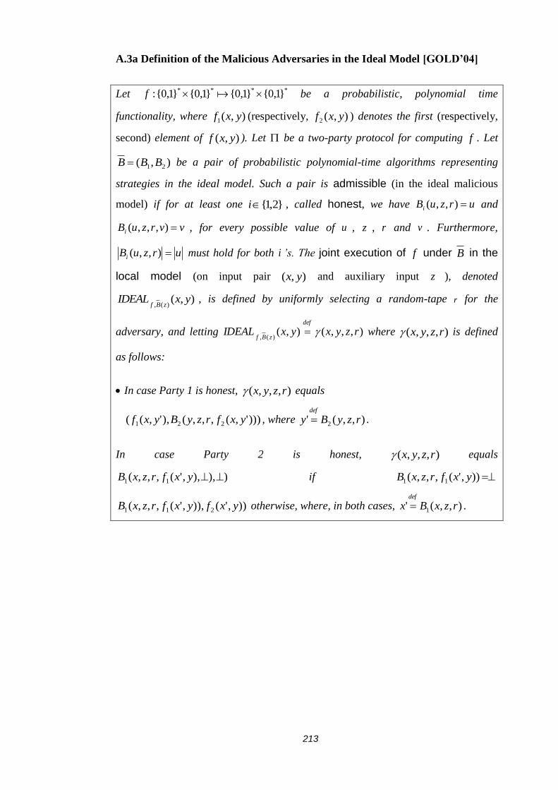
213

A.3a Definition of the Malicious Adversaries in the Ideal Model [GOLD’04]



second) element of ),( yxf ). Let be a two-party protocol for computing f . Let

),( 21 BBB be a pair of probabilistic polynomial-time algorithms representing

strategies in the ideal model. Such a pair is admissible (in the ideal malicious

model) if for at least one }2,1{i , called honest, we have urzuBi ),,( and

vvrzuBi ),,,( , for every possible value of u , z , r and v . Furthermore,

urzuBi ),,( must hold for both i ’s. The joint execution of f under B in the

local model (on input pair ),( yx and auxiliary input z ), denoted

),()(,

yxIDEALzBf

, is defined by uniformly selecting a random-tape r for the

adversary, and letting ),,,(),()(,

rzyxyxIDEALdef

zBf where ),,,( rzyx is defined

as follows:

In case Party 1 is honest, ),,,( rzyx equals

)))',(,,,(),',(( 221 yxfrzyByxf , where ),,(' 2 rzyBydef

.

In case Party 2 is honest, ),,,( rzyx equals

)),),,'(,,,( 11 yxfrzxB if )),'(,,,( 11 yxfrzxB

)),'()),,'(,,,( 211 yxfyxfrzxB otherwise, where, in both cases, ),,(' 1 rzxBxdef

.

214

A.3b Definition of the Malicious Adversaries in the Real Model [GOLD’04]



second) element of ),( yxf ). Let be a two-party protocol for computing f . Let

),( 21 AAA be a pair of probabilistic polynomial-time algorithms representing

strategies in the real model. Such a pair is admissible (with respect to ) (for the

real malicious model) if at least one iA coincides with the strategy specifies by .

(In particular, this iA ignores the auxiliary input.) The joint execution of under

A in the real model (on input pair ),( yx and auxiliary input z), denoted

),()(,

yxREALzA

is defined as the output pair resulting from the interaction between

),(1 zxA and ),(2 zyA . (Recall that the honest iA ignores the auxiliary input z , and

so our peculiar choice of providing both iA ’s with the same z is immaterial.)

215

A.3c Security in the Malicious Model [GOLD’04]



second) element of ),( yxf ). Let be a two-party protocol for computing f .

Protocol is said to securely compute f (in the malicious model) if for every

probabilistic polynomial-time pair of algorithm ),( 21 AAA that is admissible for

the real model (of Definition 2.2b), there exists a probabilistic polynomial-time pair

of algorithm ),( 21 BBB that is admissible for the ideal model (of Definition 2.2a)

such that

zyxzA

C

zyxzBfyxREALyxIDEAL ,,)(,,,)(,)},({)},({

, where

*}1,0{,, zyx , such that

yx and )( xpolyz .

(Recall that C

denotes computational indistinguishability by (non-uniform) families

of polynomial-size circuits). When the context is clear, we sometimes refer to as

a secure implementation of f .

216

A.4 The Security Definition w.r.t to Covert Adversaries. [AUMA’07]

Let 10 be a value called deterrence factor. Any attempt to cheat by an

adversary is detected by the honest parties with probability at least . Thus,

provided that is sufficient large, an adversary that wishes not to be caught

cheating, will refrain from attempting to cheat, lest it be caught doing so. Clearly,

the higher the value , the greater the probability that the adversary is caught and

thus the greater the deterrent to cheat. We therefore call out notation security in the

presence of covert adversaries with -deterrent. Note that the security guarantee

does not preclude successful cheating.

217

B. Protocol Prototypes

B.1 MATLAB.P22NSTP

% Alice.RpdfGP

% function [Dset_aug choose_Of_Random_functionX Dset_min_1 Dset_max_1

Dset_sig_1 Dset_avg_1] =step_1_alice_rpdfgp()

function [size_of_Dset_aug] = step_1_alice_rpdfgp() clear clc

%--start -- random number generation function for the joint party--------

-- X = ‘x.dat’; % call function x.dat

Dset = X; Dset_max = max(Dset); Dset_min = min(Dset); Dset_avg = mean(Dset); Dset_var = var(Dset);

% generate three random value for disguising mean&variance&max&min--- for i = 1 : 3 K_rand(i) = 1 + round(10.*rand(1,1)); %range from 1 to 10 end

Dset_avg_1 = (K_rand(1)*Dset_avg).*rand(1,1); Dset_var_1 = (K_rand(2)*Dset_var).*rand(1,1); Dset_sig_1 = sqrt(Dset_var_1); Dset_min_1 = Dset_min.*rand(1,1); Dset_max_1 = Dset_min + (K_rand(3)*Dset_max).*rand(1,1); % to make sure

Dest_max_1 is larger than Dset_min_1

for i = 4 : 5 K_rand(i) = 1 + round(10.*rand(1,1)); %range from 1 to 10, generate

further two multiplier to increase the range of random numbers. end

size_of_X = length(X);

%use uniform distribution to generate random value Generate_random_X_using_uniform = abs(round(Dset_min_1 +

Dset_max_1.*rand(1,K_rand(4)*size_of_X)));

%use normal distribution to generate random value Generate_random_X_using_normal = abs(round(Dset_avg_1 +

Dset_sig_1.*randn(1,K_rand(4)*size_of_X))); %--end -- random number generation function for Alice-------------

choose_Of_Random_functionX = round(rand(1,1)); if choose_Of_Random_functionX == 1 Dset_aug = [Dset Generate_random_X_using_uniform]; else Dset_aug = [Dset Generate_random_X_using_normal]; end

218

size_of_Dset_aug = size(Dset_aug,2);

save Dset Dset; save Dset_aug Dset_aug; save Dset_avg_1 Dset_avg_1 save Dset_var_1 Dset_var_1 save Dset_sig_1 Dset_sig_1 save Dset_min_1 Dset_min_1 save Dset_max_1 Dset_max_1 save choose_Of_Random_functionX choose_Of_Random_functionX

%row_size_of_Dset_aug_step_1_alice_rpdfgp = size(Dset_aug,1); %column_size_of_Dset_aug_step_1_alice_rpdfgp = size(Dset_aug,2); %size_of_Dset_step_1_alice_rpdfgp = size(Dset,2);

219

% Alice.DOP

% function [Task_1_Result permutation_Matrix_1]

=step_2_alice_dop(Dset_aug, choose_Of_Random_functionX, Dset_min_1,

Dset_max_1, Dset_sig_1, Dset_avg_1)

function [rowsize_of_Task_1_Result,

colsize_of_Task_1_Result]=step_2_alice_dop() clear clc

load('Dset.mat'); load('Dset_aug.mat'); load('choose_Of_Random_functionX.mat'); load('Dset_min_1'); load('Dset_max_1'); load('Dset_sig_1'); load('Dset_avg_1');

%first stage permutation matrix, generate permutation matrix 1

Length_of_Dset_aug = length(Dset_aug); % permutation matrix 1 is used to swap the order of xi and xi', it

only % makes this computation smooth, it doesn't contribute any security % protection, cause it has to be sent to Bob at the later stage.

permutation_Matrix_1 = eye(Length_of_Dset_aug,Length_of_Dset_aug); for i=1 : Length_of_Dset_aug index = round( 1 + (Length_of_Dset_aug-1).*rand(2,1)); temp1 = zeros(Length_of_Dset_aug,1); temp1 = permutation_Matrix_1(:,index(1)); permutation_Matrix_1(:,index(1)) =

permutation_Matrix_1(:,index(2)); permutation_Matrix_1(:,index(2)) = temp1; end %in this step, I generate an eye matrix first, then swap the column

of this %eye matrix, need to think is this method ok? does this method come

with %any weakness?

Dset_aug_permuted_by_permutation_Matrix_1 = (Dset_aug *

permutation_Matrix_1);

Permuted_diagonal_Matrix =

zeros(Length_of_Dset_aug,Length_of_Dset_aug); for i = 1 : Length_of_Dset_aug Permuted_diagonal_Matrix(i,i) =

Dset_aug_permuted_by_permutation_Matrix_1(i); end

%generate random matrix M, it is either generated by normal

distribution or %uniform distribution according to the previous computation result

rand_number_Matrix = zeros(Length_of_Dset_aug,Length_of_Dset_aug); if choose_Of_Random_functionX == 1 for i = 1 : Length_of_Dset_aug for j = 1 : Length_of_Dset_aug rand_number_Matrix(i , j) = abs(round(Dset_min_1 +

220

Dset_max_1.*rand(1,1))); end end else for i = 1 : Length_of_Dset_aug for j = 1 : Length_of_Dset_aug rand_number_Matrix(i , j) = abs(round(Dset_avg_1 +

Dset_sig_1.*randn(1,1))); end end end % to make the diagonal entry to be 0. for i = 1 : Length_of_Dset_aug rand_number_Matrix(i,i) = 0; end

Step_1_ranndomized_matrix = rand_number_Matrix +

Permuted_diagonal_Matrix;

% the permutation matrix 2 is used to swap the order of row order

of xi', % it is used later to generate the table to record the swap order

of this % permutation.

permutation_Matrix_2 = eye (Length_of_Dset_aug,Length_of_Dset_aug); for i=1 : Length_of_Dset_aug index = round( 1 + (Length_of_Dset_aug-1).*rand(2,1)); temp2 = zeros(Length_of_Dset_aug,1); temp2 = permutation_Matrix_2(:,index(1)); permutation_Matrix_2(:,index(1)) =

permutation_Matrix_2(:,index(2)) ; permutation_Matrix_2(:,index(2)) = temp2; end

Task_1_Result = permutation_Matrix_2 * Step_1_ranndomized_matrix;

% this step is to record the swap of order changed by permutation

matrix 1 for i = 1:length(permutation_Matrix_1) row_swap_order_by_pM1(i) = find (permutation_Matrix_1(i,:));

%to find the row to where xi is swapped by T1 column_swap_order_by_pM1(i) = find (permutation_Matrix_1(:,i));

% to find the column to where xi is swapped by T1 end

% this step is to record the swap of order changed by permutation

matrix 2. for i = 1:length(permutation_Matrix_2) row_swap_order_by_pM2(i) = find (permutation_Matrix_2(i,:));

%to find the row to where xi' is swapped by T2 column_swap_order_by_pM2(i) = find (permutation_Matrix_2(:,i));

% to find the column to where xi' is swapped by T2 end

rowsize_of_Task_1_Result = size(Task_1_Result,1); colsize_of_Task_1_Result = size(Task_1_Result,2);

save Task_1_Result Task_1_Result; save permutation_Matrix_1 permutation_Matrix_1; save permutation_Matrix_2 permutation_Matrix_2; save row_swap_order_by_pM1 row_swap_order_by_pM1;

221

save column_swap_order_by_pM1 column_swap_order_by_pM1; save row_swap_order_by_pM2 row_swap_order_by_pM2; save column_swap_order_by_pM2 column_swap_order_by_pM2;

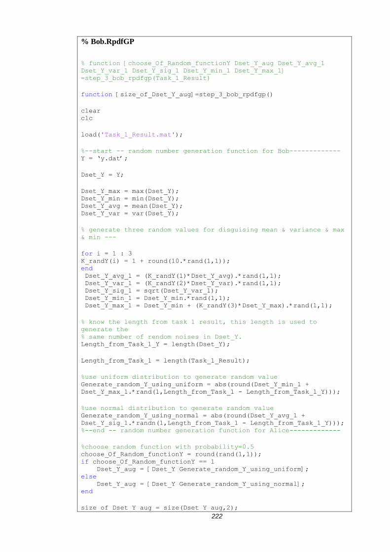
222

% Bob.RpdfGP

% function [choose_Of_Random_functionY Dset_Y_aug Dset_Y_avg_1

Dset_Y_var_1 Dset_Y_sig_1 Dset_Y_min_1 Dset_Y_max_1]

=step_3_bob_rpdfgp(Task_1_Result)

function [size_of_Dset_Y_aug]=step_3_bob_rpdfgp()

clear clc

load('Task_1_Result.mat');

%--start -- random number generation function for Bob------------- Y = ‘y.dat’;

Dset_Y = Y;

Dset_Y_max = max(Dset_Y); Dset_Y_min = min(Dset_Y); Dset_Y_avg = mean(Dset_Y); Dset_Y_var = var(Dset_Y);

% generate three random values for disguising mean & variance & max

& min ---

for i = 1 : 3 K_randY(i) = 1 + round(10.*rand(1,1)); end Dset_Y_avg_1 = (K_randY(1)*Dset_Y_avg).*rand(1,1); Dset_Y_var_1 = (K_randY(2)*Dset_Y_var).*rand(1,1); Dset_Y_sig_1 = sqrt(Dset_Y_var_1); Dset_Y_min_1 = Dset_Y_min.*rand(1,1); Dset_Y_max_1 = Dset_Y_min + (K_randY(3)*Dset_Y_max).*rand(1,1);

% know the length from task 1 result, this length is used to

generate the % same number of rendom noises in Dset_Y. Length_from_Task_1_Y = length(Dset_Y);

Length_from_Task_1 = length(Task_1_Result);

%use uniform distribution to generate random value Generate_random_Y_using_uniform = abs(round(Dset_Y_min_1 +

Dset_Y_max_1.*rand(1,Length_from_Task_1 - Length_from_Task_1_Y)));

%use normal distribution to generate random value Generate_random_Y_using_normal = abs(round(Dset_Y_avg_1 +

Dset_Y_sig_1.*randn(1,Length_from_Task_1 - Length_from_Task_1_Y))); %--end -- random number generation function for Alice-------------

%choose random function with probability=0.5 choose_Of_Random_functionY = round(rand(1,1)); if choose_Of_Random_functionY == 1 Dset_Y_aug = [Dset_Y Generate_random_Y_using_uniform]; else Dset_Y_aug = [Dset_Y Generate_random_Y_using_normal]; end

size_of_Dset_Y_aug = size(Dset_Y_aug,2);

223

save choose_Of_Random_functionY choose_Of_Random_functionY; save Dset_Y Dset_Y; save Dset_Y_aug Dset_Y_aug; save Dset_Y_avg_1 Dset_Y_avg_1; save Dset_Y_var_1 Dset_Y_var_1; save Dset_Y_sig_1 Dset_Y_sig_1; save Dset_Y_min_1 Dset_Y_min_1; save Dset_Y_max_1 Dset_Y_max_1;

save Length_from_Task_1 Length_from_Task_1;

224

% Bob STCP

% function[]=step_4_bob_stcp(Dset_Y_aug, permutation_Matrix_1,

Task_1_Result)

function[rowsize_of_STCP_Result, colsize_of_STCP_Result,

num_of_STCP_Result]=step_4_bob_stcp() clear clc

load('Dset_Y_aug.mat'); load('permutation_Matrix_1.mat'); load('Task_1_Result.mat'); load('Length_from_Task_1.mat')

%Bob use permutation matrix 1 from Alice to permute Dset_Y_aug Dset_Y_aug_permuted_by_permutation_Matrix_1 = Dset_Y_aug *

permutation_Matrix_1;

%according to the length from X(Dset), Bob generates the same quantity of %replicated rows Dset_Y_aug_permuted_replicated =

repmat(Dset_Y_aug_permuted_by_permutation_Matrix_1,Length_from_Task_1,1);

%Bob computes the differences between Dset_Y_aug and task_1 DiffMatrix_Task_1_Result_Dset_Y_aug_permuted_replicated = Task_1_Result -

Dset_Y_aug_permuted_replicated;

%using data transformation technique to generate P,Q,R positive_Result = [1;0;0]; zero_Result = [0;1;0]; negative_Result = [0;0;1];

number_Of_Rows =

size(DiffMatrix_Task_1_Result_Dset_Y_aug_permuted_replicated,1); number_Of_Columns =

size(DiffMatrix_Task_1_Result_Dset_Y_aug_permuted_replicated,2);

% each comparison result will be a column vector in relation to P,Q,R. Comparison_result_Matix_for_each_Row = zeros(3, number_Of_Columns,

number_Of_Rows);

for i=1 : number_Of_Rows result_posi =

find(DiffMatrix_Task_1_Result_Dset_Y_aug_permuted_replicated(i,:)>0); result_zero =

find(DiffMatrix_Task_1_Result_Dset_Y_aug_permuted_replicated(i,:)==0); result_nega =

find(DiffMatrix_Task_1_Result_Dset_Y_aug_permuted_replicated(i,:)<0); for j=1 : number_Of_Columns if DiffMatrix_Task_1_Result_Dset_Y_aug_permuted_replicated(i,j) >

0 Comparison_result_Matix_for_each_Row(1,j,i) = 1; elseif

DiffMatrix_Task_1_Result_Dset_Y_aug_permuted_replicated(i,j) < 0 Comparison_result_Matix_for_each_Row(3,j,i) = 1; else Comparison_result_Matix_for_each_Row(2,j,i) = 1; end end end

225

for i = 4 : 4 K_randY(i) = 1 + round(10.*rand(1,1));%K_randY(4), times 10. end

%choose security parameter Length_of_added_column = round(number_Of_Rows +

K_randY(4)*number_Of_Rows.*rand(1,1));

%generate random noise matrices, for case n<=400, these random noises are %either 0 or 1, to fill the below part of the DiffMatrix.

Added_Random_Matrix = zeros(Length_of_added_column, number_Of_Rows,

number_Of_Columns);

for i=1 : Length_of_added_column for j=1: number_Of_Rows for k=1 : number_Of_Columns Added_Random_Matrix(i,j,k) = round( 1 + rand(1,1)) - 1; end end end

for i = 1 : number_Of_Columns Randomized_DiffMatrix{i}=

[Comparison_result_Matix_for_each_Row(:,:,i);Added_Random_Matrix(:,:,i)]; end

%generate permutation matrix 3 to permute the 'Randomized_DiffMatrix's permutation_Matrix_3 = eye(Length_of_added_column + 3,

Length_of_added_column + 3); for i=1 : Length_of_added_column + 3 index = round( 1 + (Length_of_added_column + 3 - 1).*rand(2,1)); temp = zeros(Length_of_added_column + 3,1); temp = permutation_Matrix_3(:,index(1)); permutation_Matrix_3(:,index(1)) = permutation_Matrix_3(:,index(2)) ; permutation_Matrix_3(:,index(2)) = temp; end

%permute every 'Randomized_DiffMatrix's by permutation matrix 3 STCP_Result = zeros(Length_of_added_column + 3, number_Of_Columns,

number_Of_Rows); for i = 1 : number_Of_Rows STCP_Result(:,:,i) = permutation_Matrix_3 * Randomized_DiffMatrix{i} end

% to record the swap order changed by permutation matrix 3 for i = 1:length(permutation_Matrix_3) row_swap_order_by_pM3(i) = find (permutation_Matrix_3(i,:)); %to find

the row to where xi is swapped by T3 column_swap_order_by_pM3(i) = find (permutation_Matrix_3(:,i)); % to

find the column to where xi is swapped by T3 end

rowsize_of_STCP_Result = size(STCP_Result,1); colsize_of_STCP_Result = size(STCP_Result,2); num_of_STCP_Result = number_Of_Rows;

save STCP_Result STCP_Result; save row_swap_order_by_pM3 row_swap_order_by_pM3; save column_swap_order_by_pM3 column_swap_order_by_pM3;

226

% Alice.DEP

function[size_of_Sum_of_Summation_Difference_2]=step_5_alice_dep()

clear clc

load('STCP_Result.mat'); load('row_swap_order_by_pM2'); load('Dset.mat'); load('column_swap_order_by_pM1.mat');

% to pick up the column vectors where xi' is located, and combine

these vectors % into a matrix. this matrix is used to computa the possible sign

test results from all possible PQR combination. %

% find the columns of all xi' from STCP result Summation_Difference =

zeros(length(STCP_Result(:,1,1)),length(STCP_Result(1,:,1))); for i = 1 : length(STCP_Result(1,:,1)) Summation_Difference(:,row_swap_order_by_pM2(i)) =

STCP_Result(:,row_swap_order_by_pM2(i),i) end

% find the columns of all xi from Summation_difference Summation_Difference_2 =

zeros(length(Summation_Difference(:,1)),length(Dset)); for i = 1 : length(Dset) Summation_Difference_2(:,i) =

Summation_Difference(:,column_swap_order_by_pM1(i)) end

% calculate the possible values of P Q R... Sum_of_Summation_Difference_2 =

zeros(1,length(Summation_Difference_2)) for i = 1 : length(Summation_Difference_2) Sum_of_Summation_Difference_2(i) =

sum(Summation_Difference_2(i,:)); end

size_of_Sum_of_Summation_Difference_2 =

size(Sum_of_Summation_Difference_2,2);

save Sum_of_Summation_Difference_2 Sum_of_Summation_Difference_2;

227

% Bob.PRP

function[p,h]=step_6_bob_prp()

clear clc

load('Sum_of_Summation_Difference_2.mat') load('column_swap_order_by_pM3.mat') load('Dset_Y.mat')

index_of_real_PQR = zeros(1,3); for i = 1 : 3 index_of_real_PQR(i) = column_swap_order_by_pM3(i) end

P = Sum_of_Summation_Difference_2(index_of_real_PQR(:,1)); Q = Sum_of_Summation_Difference_2(index_of_real_PQR(:,2)); R = Sum_of_Summation_Difference_2(index_of_real_PQR(:,3));

% transform into matlab's sign test form. Test_X = zeros(1,length(Dset_Y)); for i = 1 : P Test_X(i) = 1 end for i = P+1 : P+Q+R Test_X(i) = 0 end

Test_Y = zeros(1,length(Dset_Y)); for i = 1 : P+Q Test_Y(i) = 0 end for i = P+Q+1 : P+Q+R Test_Y(i) = 1 end

[p,h] = signtest(Test_X,Test_Y);

save p p;

save h h;

228

B.2 MATLAB.P22NSTC

% Matlab.Main.P22NSTC

a = ‘x.dat’;

b = ‘y.dat’;

nElement = size(a,2);

javaclasspath ({'c:\'});

seckey = generate.Paillier.PrivateKey(128); pubkey = seckey.generatePublicKey();

%The encryption of X by Alice tic; for i=1 : nElement eni_x(i) =

generate.Paillier.Encryption(java.prog(a(i)),pubkey); end

%The encryption of Y by Bob

for i=1 : nElement eni_y(i) =

generate.Paillier.Encryption(java.prog(b(i)),pubkey); end TIME.encrypt = toc;

%End of encryption

229

% STTP.DSP

% DSP start by STTP tic; nElementLow = round(nElement/3); nElementUpper = round(2*nElement/3); % number of n1 nElementNewA = round(nElementLow + (nElementUpper-

nElementLow).*rand(1)); % number of n2 nElementNewB = nElement - nElementNewA; PMVector1 = randperm(nElement); for i = 1 : nElementNewA NewA(i) = a(PMVector1(i)); end for i = 1 : nElementNewB NewB(i) = a(PMVector1(i + nElementNewA)); end TIME.dsp = toc; % DSP end

tic

230

% STTP.DRP for Alice

% STTP does DRP for Alice % number of n1' nElementNewAA = round(round(nElementNewA*nElementNewA/2) +

(nElementNewA*nElementNewA - nElementNewA -

round(nElementNewA*nElementNewA/2)).*rand(1)); % generate indices for ti and ui for i = 1 : nElementNewAA indexT1(i) = round(1 + (nElementNewA-1).*rand(1)); indexU1(i) = round(1 + (nElementNewA-1).*rand(1)); end % generate new noise items for i = 1 : nElementNewAA NewAA(i) = NewA(indexT1(i)) + NewA(indexU1(i)); end NewAAA = [NewA NewAA]; nElementNewAAA = size(NewAAA,2); % permute the NewAAA PMVectorAAA = randperm(nElementNewAAA); for i = 1 : nElementNewAAA permNewAAA(i) = NewAAA(PMVectorAAA(i)); end % End of DRP for Alice

231

% STTP.DRP for Bob

% STTP does DRP for Bob % number of n2' nElementNewBB = round(round(nElementNewB*nElementNewB/2) +

(nElementNewB*nElementNewB - nElementNewB -

round(nElementNewB*nElementNewB/2)).*rand(1)); % generate indices for ti and ui for i = 1 : nElementNewBB indexT2(i) = round(1 + (nElementNewA-1).*rand(1)); indexU2(i) = round(1 + (nElementNewA-1).*rand(1)); end % generate new noise items for i = 1 : nElementNewBB NewBB(i) = NewB(indexT2(i)) + NewB(indexU2(i)); end NewBBB = [NewB NewBB]; nElementNewBBB = size(NewBBB,2); % permute the NewBBB PMVectorBBB = randperm(nElementNewBBB); for i = 1 : nElementNewBBB permNewBBB(i) = NewBBB(PMVectorBBB(i)); end % End of DRP for Bob TIME.drp = toc;

% individual decrypt time by Alice and Bob, encrypt time = decrypt

time TIME.decryptAAA = (TIME.encrypt/nElement)*(nElementNewA +

nElementNewAA)*2; TIME.decryptBBB = (TIME.encrypt/nElement)*(nElementNewB +

nElementNewBB)*2;

% Additively homomorphic operation tic; for i=1 : nElement eni_xy(i) = eni_x(i).multi(eni_y(i)); end Time.cipheraddition = toc; % End of Additively homomorphic operation

tic % Data Transformation % Data Transformation for NewAAA by Alice for i = 1 : nElementNewAAA if NewAAA(i) > 0 TRMNewAAA(1,i) = 1; elseif NewAAA(i) < 0 TRMNewAAA(3,i) = 1; else TRMNewAAA(2,i) = 1; end end

% Data Transformation for NewBBB by Bob for i = 1 : nElementNewBBB if NewBBB(i) > 0 TRMNewBBB(1,i) = 1; elseif NewBBB(i) < 0 TRMNewBBB(3,i) = 1; else TRMNewBBB(2,i) = 1;

232

end end TIME.transformation = toc;

tic; % restore NewAAA order PMVectorAAA2 = randperm(nElementNewAAA); for i = 1 : nElementNewAAA permNewAAA2(i) = NewAAA(PMVectorAAA2(i)); end

% restore NewBBB order PMVectorBBB2 = randperm(nElementNewBBB); for i = 1 : nElementNewBBB permNewBBB2(i) = NewBBB(PMVectorBBB2(i)); end TIME.restore = toc;

tic % calaulate PQR & sign test P = sum (a); Q = sum (a); R = sum (a); TIME.pqr = toc;

tic; p = signtest (a,b); TIME.signtest = toc;

TIME.total = TIME.encrypt + TIME.dsp + TIME.drp + TIME.decryptAAA +

TIME.decryptBBB + TIME.transformation + TIME.restore + TIME.pqr +

TIME.signtest;

Achieving Privacy-preserving Distributed Statistical Computation

Documents

Transcript of Achieving Privacy-preserving Distributed Statistical Computation