
Tilburg University Four essays in mathematical philosophy ...
134
Tilburg University Four essays in mathematical philosophy Rafiee Rad, S. Publication date: 2014 Document Version Publisher's PDF, also known as Version of record Link to publication in Tilburg University Research Portal Citation for published version (APA): Rafiee Rad, S. (2014). Four essays in mathematical philosophy. Tilburg University. General rights Copyright and moral rights for the publications made accessible in the public portal are retained by the authors and/or other copyright owners and it is a condition of accessing publications that users recognise and abide by the legal requirements associated with these rights. • Users may download and print one copy of any publication from the public portal for the purpose of private study or research. • You may not further distribute the material or use it for any profit-making activity or commercial gain • You may freely distribute the URL identifying the publication in the public portal Take down policy If you believe that this document breaches copyright please contact us providing details, and we will remove access to the work immediately and investigate your claim. Download date: 15. Mar. 2022
-
Upload
khangminh22 -
Category
Documents
-
view
0 -
download
0
Transcript of Tilburg University Four essays in mathematical philosophy ...

Tilburg University
Four essays in mathematical philosophy
Rafiee Rad, S.
Publication date:2014
Document VersionPublisher's PDF, also known as Version of record
Link to publication in Tilburg University Research Portal
Citation for published version (APA):Rafiee Rad, S. (2014). Four essays in mathematical philosophy. Tilburg University.
General rightsCopyright and moral rights for the publications made accessible in the public portal are retained by the authors and/or other copyright ownersand it is a condition of accessing publications that users recognise and abide by the legal requirements associated with these rights.
• Users may download and print one copy of any publication from the public portal for the purpose of private study or research. • You may not further distribute the material or use it for any profit-making activity or commercial gain • You may freely distribute the URL identifying the publication in the public portal
Take down policyIf you believe that this document breaches copyright please contact us providing details, and we will remove access to the work immediatelyand investigate your claim.
Download date: 15. Mar. 2022

.

.

Four Essays
in Mathematical Philosophy
Proefschrift
ter verkrijging van de graad van doctoraan Tilburg University
op gezag van de rector magnificus,prof. dr. Ph. Eijlander,
in het openbaar te verdedigen ten overstaan van eendoor het college voor promoties aangewezen commissie
in de aula van de Universiteit
op maandag 29 september 2014 om 10.15 uur
door
Soroush Rafiee Rad
geboren op 22 juli 1981 te Tehran, Iran

Promotiecommissie
Promotor: prof. dr. S. Hartmann
Overige leden van de Promotiecommissie:
prof. dr. L. Bovensprof. dr. I. Douvenprof. dr. R. Parikhdr. S. Smetsprof. dr. J. Sprenger

Acknowledgments
I would like to thank my parents for their constant support, encouragementand persuasion, for nurturing my curiosity and teaching me the value of knowl-edge, and for providing me with a lifetime of opportunities that have led to thispoint.
I would like to express special gratitude to my supervisor, Prof. Stephan Hart-mann, for his patience, inspiration, contribution and guidance, without which thiswork would not have been possible. I am grateful to him for teaching me how tothink as a philosopher and for four fruitful years of intellectual stimulation.
I would like to thank the members of my thesis committee for many construc-tive comments and suggestions that have greatly improved the work presented inthis thesis.
I am grateful to my brother Siavash for his help, support and encouragementthroughout all the years of my studies, as well as for his help in proof readingmajor parts of this thesis and for many valuable discussions that have led tomany improvements in this work.
I am also grateful to my friend Karim Thebault for very useful comments thatsignificantly improved the presentation of this thesis.
Finally I would like to thanks my friend Arash Eshghi, for endless hours ofdiscussion, for many years of intellectual stimulation and for his ever increasinglove for philosophy that has been a significant catalyst to my philosophical cu-riosity for many years. For these I am grateful to him, and the work in this thesisis directly or indirectly indebted to him.

6

7
ABSTRACT.
Scientific philosophy is a recent but rapidly growing approach to investi-gate a wide range of philosophical problems. This approach advocates theemployment of scientific methodologies, including mathematical and computa-tional methods, in philosophical investigations. In this thesis we will presentfour case studies in scientific philosophy, using both mathematical/logicalformalisations and computational simulations. We will investigate problemsfrom different philosophical disciplines aiming to show how the formal andcomputational methods can be beneficial to a wide range of philosophicalinvestigations. We shall study a probabilistic approach to para-consistencyand reasoning from conflicting information, learning indicative conditionals,modelling rational deliberation and an investigation of the anchoring effect indeliberations. All these are long standing problems in philosophy that haveattracted a lot of interest, in particular, in recent years. Thus, in this thesis, wehope to contribute to the growing literature in scientific philosophy and furthermotivate its extensive domain of application.

8
Contents
1 Introduction 11
2 Reasoning From Conflicting Information 212.1 Introduction . . . . . . . . . . . . . . . . . . . . . . . . . . . . . . . . . 21
2.1.1 Preliminaries and Notation . . . . . . . . . . . . . . . . . . . 252.2 Revising Inconsistent Evidence . . . . . . . . . . . . . . . . . . . . . 27
2.2.1 Revising Inconsistent Categorical Evidence . . . . . . . . . . 272.2.2 Revising Inconsistent Probabilistic Evidence . . . . . . . . . 292.2.3 Revising Prioritised Evidence With Degrees Of Entrenchment 30
2.3 Probabilistic Entailment . . . . . . . . . . . . . . . . . . . . . . . . . 312.3.1 The η ⊳ζ Entailment . . . . . . . . . . . . . . . . . . . . . . . 312.3.2 Properties of η ⊳ζ . . . . . . . . . . . . . . . . . . . . . . . . . 33
2.4 Generalising to Multiple Thresholds; η ⊳ζ . . . . . . . . . . . . . . . 362.5 Reasoning with Inconsistent Information . . . . . . . . . . . . . . . . 372.6 Conclusion . . . . . . . . . . . . . . . . . . . . . . . . . . . . . . . . . . 382.7 Appendix . . . . . . . . . . . . . . . . . . . . . . . . . . . . . . . . . . 39
2.7.1 A Classical Analysis of η ⊳ζ . . . . . . . . . . . . . . . . . . . 39
3 Learning Indicative Conditionals 473.1 Introduction . . . . . . . . . . . . . . . . . . . . . . . . . . . . . . . . . 473.2 The Kullback-Leibler Divergence and Probabilistic Updating . . . 483.3 Meeting the Challenges . . . . . . . . . . . . . . . . . . . . . . . . . . 56
3.3.1 The Sundowners Example . . . . . . . . . . . . . . . . . . . . 573.3.2 The Ski Trip Example . . . . . . . . . . . . . . . . . . . . . . 593.3.3 The Driving Test Example . . . . . . . . . . . . . . . . . . . . 623.3.4 The Judy Benjamin Problem . . . . . . . . . . . . . . . . . . 64
3.4 Disabling Conditions . . . . . . . . . . . . . . . . . . . . . . . . . . . . 663.5 Conclusion . . . . . . . . . . . . . . . . . . . . . . . . . . . . . . . . . . 693.6 Appendix . . . . . . . . . . . . . . . . . . . . . . . . . . . . . . . . . . 69
3.6.1 Three Lemmata . . . . . . . . . . . . . . . . . . . . . . . . . . 69
9
10 CONTENTS
3.6.2 Theorem 1 . . . . . . . . . . . . . . . . . . . . . . . . . . . . . 703.6.3 Theorem 2 . . . . . . . . . . . . . . . . . . . . . . . . . . . . . 713.6.4 Theorem 3 . . . . . . . . . . . . . . . . . . . . . . . . . . . . . 723.6.5 Proposition 1 . . . . . . . . . . . . . . . . . . . . . . . . . . . . 743.6.6 Proposition 2 . . . . . . . . . . . . . . . . . . . . . . . . . . . . 743.6.7 Theorem 4 . . . . . . . . . . . . . . . . . . . . . . . . . . . . . 753.6.8 Theorem 5 . . . . . . . . . . . . . . . . . . . . . . . . . . . . . 79
4 Voting, Deliberation And Truth 814.1 Introduction . . . . . . . . . . . . . . . . . . . . . . . . . . . . . . . . . 814.2 A Bayesian Model of Deliberation . . . . . . . . . . . . . . . . . . . . 85
4.2.1 The Deliberation Procedure . . . . . . . . . . . . . . . . . . . 864.3 Homogeneous Groups . . . . . . . . . . . . . . . . . . . . . . . . . . . 88
4.3.1 Comparison with Majority Voting . . . . . . . . . . . . . . . 904.4 Inhomogeneous Groups . . . . . . . . . . . . . . . . . . . . . . . . . . 91
4.4.1 Truth Tracking . . . . . . . . . . . . . . . . . . . . . . . . . . . 934.4.2 Comparison with Majority Voting . . . . . . . . . . . . . . . 94
4.5 Conclusions . . . . . . . . . . . . . . . . . . . . . . . . . . . . . . . . . 964.6 Appendix . . . . . . . . . . . . . . . . . . . . . . . . . . . . . . . . . . 98
5 Anchoring In Deliberations 1015.1 Introduction . . . . . . . . . . . . . . . . . . . . . . . . . . . . . . . . . 1015.2 Modeling Anchoring . . . . . . . . . . . . . . . . . . . . . . . . . . . . 103
5.2.1 The Estimation of Reliabilities . . . . . . . . . . . . . . . . . 1055.2.2 The Updating Procedure . . . . . . . . . . . . . . . . . . . . . 106
5.3 The Anchoring Effect in Deliberations . . . . . . . . . . . . . . . . . 1075.3.1 Homogeneous Groups . . . . . . . . . . . . . . . . . . . . . . . 1085.3.2 Inhomogeneous Groups . . . . . . . . . . . . . . . . . . . . . . 109
5.4 Conclusion . . . . . . . . . . . . . . . . . . . . . . . . . . . . . . . . . . 1155.5 Appendix . . . . . . . . . . . . . . . . . . . . . . . . . . . . . . . . . . 115
5.5.1 Proof of Theorem 5.3.2 . . . . . . . . . . . . . . . . . . . . . . 1155.5.2 Stability Result . . . . . . . . . . . . . . . . . . . . . . . . . . 119
6 Conclusion 125
Chapter 1
Introduction
Scientific philosophy is a relatively new approach to philosophical enquiry thatamidst, sometimes strongly voiced, oppositions and supports is increasingly gain-ing popularity in the recent years. According to Leitgeb (Leitgeb 2013) there areat least three ways to understand scientific philosophy.
The first view goes back to the ideas of the Vienna and the Berlin circles andconsiders philosophy as a discipline employed in the service of science. On thisview, the role of philosophy is to study and analyse science on the meta-level.The goal of philosophy will then be to refine and improve scientific language andto enhance the logic where needed and possible. The study of scientific fieldson the meta-level clarifies and improves our understanding of the concepts thatplay a part in the corresponding scientific field and their interrelation. In doingso, philosophy contributes to the development of an appropriate object languagewith which scientists work and the adoption of the correct logical structures andreasoning mechanisms suitable for different scientific theories. The contributionof philosophy in this view, as advocated by Michael Friedman for example, is mostvisible in Kuhnian paradigm shifts when a new scientific theory replaces an oldone. At such revolutionary stages, philosophy plays a crucial role in developmentof proper scientific language and is the force that ensures the scientific theorychange remains confined within the boundaries of rationality.
The second view sees philosophical studies as part of the scientific endeav-our. This account, advocated amongst others by Quine, roots in Naturalismand considers natural sciences our best medium to access the truth and so themost viable approach to philosophical studies. According to this view, the roleof philosophy is to analyse and shed light on the foundational issues in scien-tific disciplines and the philosophical studies should be carried out along thesame methodological lines, in the same language as in the respective scientific
11
12 CHAPTER 1. INTRODUCTION
fields and by employment and use of scientific theories and their results. Quine’snaturalised epistemology, for example, emphasises the close connection betweenepistemology and natural sciences and the necessity to take into account theresults from the study of human reasoning when dealing with problems in episte-mology. In his view, our knowledge can be captured mainly in our language use,the observable characteristics of which allows its study in the same manner asother scientific inquiries. This account closely connects the study of epistemologywith research in cognitive psychology and argues in favour of articulating prob-lems and arguments in epistemology using the language and concepts developedin psychology. As pointed out by Leitgeb (Leitgeb 2013), philosophy of mathe-matics and set theory as well as studies in metaphysics and physics, for example,bear the same connection and in this conception of scientific philosophy shouldbe carried out in the same languages respectively and deal with the same issuesand concerns. Thus this view urges (or in more radical approaches, necessitates)the employment and use of scientific theories and the results of investigations inrelevant scientific disciplines for proper and fruitful study of philosophical ques-tions. This approach has been taken up in more recent years by philosopherssuch as Penelope Maddy in her book “Second Philosophy” (Maddy 2009), andJames Ladyman and Don Ross in their account of naturalistic metaphysics in“Every Thing Must Go: Metaphysics Naturalized” (Ladyman & Ross 2009) whohave argued for naturalisations of parts of philosophy.
Finally the third view, understands scientific philosophy as the philosophycarried out using scientific methods. This is the account of scientific philosophythat this thesis will fall into. As emphasised by Leitgeb, this account is in noconflict with viewing philosophy as an independent discipline that is “not neces-sarily being pursued, whether on the meta-level or on the object level, with theaim of facilitating scientific progress” (Leitgeb 2013). Thus with this account ofscientific philosophy, philosophers are no more required (at least not necessarily)to be concerned with problems and notions raised in scientific theories and phi-losophy is an autonomous discipline with its own concepts and questions. Thisview is thus consistent with philosophy as a discipline that is pursued for thesake of understanding issues and concerns that stem from motivations other thanscientific progress and that have engaged our forefathers since antiquity; issuessuch as truth, knowledge, existence, morality and ethics.
What, then, are the scientific methods that that can be employed in philo-sophical studies? As hard as it may be to clearly characterise what can or cannotbe considered as scientific methods useful for philosophy, there are some obvi-ous candidates to start with. In (Leitgeb 2013), for instance, Leitgeb points tothree examples, namely, mathematical, computational and experimental meth-ods. First are the mathematical methods. Mathematical methods have been inuse in scientific studies for as long as such studies have been carried out. Their
13
employment in philosophy is also old news. Application and study of mathe-matical logic in philosophical studies, for example, dates back to works of Aris-totle. Leibniz work on metaphysics is another example in point. The link hasgrown stronger in the more contemporary studies in philosophy by introductionof inductive logic, temporal logics, epistemic logics, dynamic logics and the like.The connection, however, does not end with mathematical logic and includesa wide range of mathematical disciplines such as probability theory, game the-ory, discrete mathematics, etc. The interplay of philosophy and mathematics inthe investigation of mechanisms for reasoning, in particular, has brought aboutthriving research programs that have continued throughout the 20th century andis continuing to this date. An impressive collection of works in the literature,commonly referred to as Formal Philosophy is witness to this thriving dynamics.The formal Epistemology movement and the birth and formulation of BayesianEpistemology are examples in point.
Second are the computational methods. This is, in short, application ofcomputational algorithms, computer simulations and the resulting numericalanalysis in the study of philosophical problems and in support of philosoph-ical claims and arguments. Computational models, for example, have beenused for more than two decades to study both the process of scientific dis-covery and the process of evaluating scientific theories. The BACON project,a pioneering project in this regard, for instance, was developed by Pat Lan-gley, Herbert Simon and their colleagues (Langley et. al. 1987 ) as model forderiving mathematical laws from numerical data. Other examples are theKEKADA program developed by Kulkarni and Simon (Kulkarni & Simon 1988)and Paul Thagard ”Computational Philosophy of Science” (Thagard 1993),that introduces a computational model for problem solving which he usesto study issues in philosophy of science such as hypothesis formation andtheory justification amongst others. The Structure Mapping Engine devel-oped by Falkenhainer, Forbus, and Gentner (Falkenhainer et. al. 1989), theAnalogical Constraint Mapping Engine introduced by Holyoak and Thagard(Holyoak & Thagard 1989; Holyoak & Thagard 1995) for modelling anologicalreasoning and the ECHO program developed by Thagard to model theory evalua-tion in science are other examples of computational approaches as is the Fitelson’sand Zelta’s (Fitelson & Zalta 2007) work on computational metaphysics.
More recently, there has been many examples of the application of computersimulations, in particular formal epistemology and in philosophy of social sci-ences. This is, at least, partly because these simulations prove very useful instudying the group dynamics and the emergence and evolution of phenomenain social interactions. Many instances of (emergence or dissolution of) socialphenomena or patterns in groups depend on the group topology and the connec-tions between individuals in the group. This makes the analytical study of such
14 CHAPTER 1. INTRODUCTION
instances difficult in the sense that many different cases have to be consideredseparately. Computer simulations allow study of diverse large sample spaces toidentify common trends that that can be studied uniformly among different cases.Not only are computer simulations increasingly used in philosophical studies, buttheir application has become significant enough to prompt philosophical studiesinto simulations themselves. These studies, for instance “Computer Simulationsand the Changing Face of Scientific Experimentation” by Juan Duran and Eck-hart Arnold (Duran & Arnold 2013), are aimed to better understand the type ofinference that is possible on the basis of computer simulations and the criteriathat constitute a conceptually adequate simulation.
Third kind of scientific methods, are the experimental methods. Experimen-tal philosophy uses empirical data gathered through surveys, interviews and de-signed experiments to derive clues with regard to philosophical questions. Theissue of using such methods is the subject of intense debate among philosophers.Although the empirical studies appear to be illuminating and insightful for philo-sophical studies in many instances, in particular, investigations in philosophy ofmind, philosophy of language, morality and the like, for example in the works ofNatalie Gold, Regina Rini, Stephen Stich, Shen-yi Liao among others, there hasbeen serious criticisms raised in opposition to it. One immediate reason is that,as opposed to computational and mathematical methods, empirical results doesnot provide a priori knowledge or justification. Another point of criticism is thatpeople’s intuitions, which are the main outcome of experimental studies, cannotbe considered as evidence for philosophical studies. Thus, the use of experimentalmethods is more controversial than the formal and computational methods andwe shall not be concerned with them in this thesis.
There are many reasons as to why the application of formal methods is usefulin philosophy. An important contribution of mathematical methods is the expli-cation of philosophical concepts. This is the development of new concepts thatcan extend existing concepts in the sense that the new concept coincides with theold in standard and clear cases while improving on it in “exactness, fruitfulnessand simplicity”, see (Leitgeb 2013), in the more problematic or fuzzy cases. In(Leitgeb 2013) Leitgeb argues that not only are the mathematical formulationsuseful for the process of explicating philosophical concepts but they are in manycases necessary. Tarski’s explication of truth, Carnap’s explication of confirma-tion of hypotheses by evidence, and Adams’ explication of the acceptability ofconditionals are examples of such cases. Tarski’s work is built on second orderlogic and set theory while Carnap’s and Adams’ require the theory of subjectiveprobability. In addition, mathematical definitions and formulation, where pos-sible, can make philosophical concepts more precise and immune to divergenceof interpretations. Similarly, precision and exactness of mathematical proofs canbe carried into the philosophical arguments that are formulated in mathematical
15
terms. Using mathematical language and formal methods not only makes thephilosophical arguments more precise but are also needed to represent the morecomplex arguments correctly and more understandably. The same way formalmodels are useful in presenting arguments that are not necessarily proofs in thesense of showing that the truth of assumptions entail the truth of the conclusionsbut rather inductively strong in the sense that the conclusions are at least aslikely as the assumptions. Hartmann and Bovens use of Bayesian networks in(Bovens & Hartmann 2003) in support of claims about confirmation, testimony,etc. have such characteristic. What is more, mathematical formulations willmake all the relevant assumptions and prerequisites explicit and again preventthe multitude of interpretations. They clarify links to scientific theories whichmight in turn introduce interesting new philosophical concepts or questions andeven point to enological cases in different areas of philosophy.
The benefits of such formal approaches, however, can be best evaluated bylooking at the contribution of the application of such methods to the philosophicalliterature. The role of mathematical formulation is robustness and rigidity ofBayesian epistemology, theories of truth, studies of rationality and belief revisionand investigations in social epistemology and collective rationality and decisionmaking needs no reminder. It seems, however, important to emphasise that theformal approach to philosophy is not a reductionist view. The aim is not toreduce philosophical studies to mathematics or any other scientific discipline butrather to use mathematical, computational and scientific results to the benefitof philosophical investigations where such applications are possible. This is toacknowledge that there may very well remain many areas, concepts and questionsin philosophy where it is not possible (or not yet possible) to take a formal stand.But where the application of such methods has been possible, the input andbenefit of such applications to the literature, to which we also hope to contributein this thesis, is undeniable.
What Follows....
In what follows we will present four studies in scientific philosophy in thethird sense above, using mathematical and computational methods (and theircombination). The studies are carried out in the framework of formal and socialepistemology and the first two deal with problems of reasoning for individualrational agents and the second two are concerned with issues of collective decisionmaking. All problems that we shall visit in this thesis have been of long standinginterest to philosophers and the subject of philosophical debate and investigationfor quite some time. The goal here is to demonstrate how the application offormal tools can help to settle or further elaborate these problems.
We start with the problem of para-consistent reasoning. This has attractedthe theoretical interest of logicians and philosophers for a long time and sev-
16 CHAPTER 1. INTRODUCTION
eral approaches have been proposed and studied in the literature, see for ex-ample, (da Costa 1974; da Costa 1989; da Costa 1998) (Priest 1979; Priest 1987;Priest 1989). Besides the purely theoretical interest, however, working with in-consistencies is of great importance in the study of practical reasoning. Ourapproach to para-consistency arises from the studies of probabilistic consequencerelations in (Knight 2002), (Paris 2004) and (Picado-Muino 2008). We advocatethe idea that the inconsistency in an agent’s evidence should be identified withthe uncertainty that it will induce in the agent’s knowledge. In this sense, reason-ing with inconsistent information is essentially reduced to uncertain reasoning.We will proceed in our investigation in three steps. First, we will present theformal machinery to bridge between an inconsistent set and its uncertain con-sistent reduction. Next, we will extend the approach developed in (Paris 2004)and (Paris et. al. 2008) for defining a probabilistic consequence relation, to firstorder languages. The probabilistic consequence relation will then provide the for-mal logical system for reasoning with these (consistent) uncertain knowledge sets.Finally we will briefly discuss some immediate generalisations of this approach.
Almost all current models of belief revision assign a higher degree of reliabilityto the new information than what is already in the belief set. The approachpresented in this study allows us to assign different degrees of trust to the newlyreceived information not only with respect to the current knowledge set as awhole but also with respect to each individual statement in that set. This will,thus, allow a fine graded analysis of the inconsistency in relation to the currentknowledge set and the new information.
The second study on the individual aspects of reasoning concernsthe indicative conditionals. The issue has been studied meticulously inthe works of Arlo-Costa, Lewis, Stalnaker, van Fraassen and Douvenamong others, (Arlo-Costa1990), (Douven 2012), (Douven & Romeijn 2012),(van Fraassen 1981), (Stalnaker 1968), (Lewis 1976), and several approacheshave been proposed and studied in the literature. These include identifying theindicative conditional with the corresponding material conditional, working withthe Stalnaker account using imaging as proposed by David Lewis, updating withAdam’s conditioning rule or using information theoretic updating procedures suchas Kullback-Leibler (KL) distance minimisation1.
All these proposals, however, have been criticised by means of counter exam-ples and despite the extensive effort spent on the issue, a general Bayesian accountof updating on conditionals is still missing from the literature. The essence ofthese counter examples deals with the unintuitive effect of updating procedureon the probability of the antecedent of the conditional. To be more precise, theyare all concerned with how the posterior probability of the antecedent comparesto its prior probability as the result of the updating procedure as opposed to how
1This approach was, to our knowledge, first studied by van Fraassen.
17
they should compare intuitively (see, (Douven 2012)).
We shall address this problem using existing links to measure theory and theKullback-Leibler Distance minimisation procedure, the theory of casual struc-tures and their relation to conditionals. Our proposal is the implementation ofthe KL distance minimisation in a slightly richer setting. To be more precise, wewill show that the KL distance minimisation will provide the intuitively expectedresults if applied in a setting where all the relevant variables in the scenario arefixed and the complete causal structure of the problem is identified. In this set-ting, one will start with the prior belief function induced by the causal structureand the indicative conditional will give a constraint on the posterior probabilities.The posterior probability function will then be chosen as to minimises the KLdistance to the priors. We shall revisit all the examples given by Douven and hisco-authors as well as the Judy Benjamin example and will show that the aboveproposal will give the results that one intuitively expects in all proposed scenar-ios. These two studies are concerned with aspects of reasoning and the dynamicsof belief in individual agents while the next two will deal with belief dynamics ina collective setting.
Our third study deals with the investigation of rational deliberation in groups.The expansion and multitude of different social networks, to which almost eachand every member of the society is subscribed in the modern day, is rapidly in-creasing the number of essentially social judgments. The majority of decisionsare no longer made by individual agents but rather by the social networks towhich they belong and as such, are inevitably subject to influence and revisionas they evolve from personal judgments into a collective decisions. This evolu-tion takes place, to a major part, in the course of agents social interactions andcommunications. Deliberation is an important example of such social interactionand communications and the normative investigation of mechanisms that governthe flow of deliberative processes and the dynamics of belief change towards thegroup consensus, can be instrumental in devising interaction protocols that facil-itate dissemination of some independent and inter-subjective truth, when such isdefinable. Our goal in this study is to contribute to this investigation.
Groups can proceed to make a collective decision either by aggregating indi-vidual judgments such as in voting scenarios or can deliberate on the issue untilthey reach a consensus where all the group members manifest the same individualjudgment. There are also two views on how to evaluate methods for collectivedecision making. From the proceduralist point of view, a decision making proce-dure should be judged on the basis of its procedural characteristics only withoutany reference to the epistemic nature of the outcomes. On the other hand is theepistemic view that evaluates a decision making process by the epistemic valuesof its outcomes without taking account of the procedural considerations. In caseof democratic decision making, the distinction between the two conceptions can
18 CHAPTER 1. INTRODUCTION
be formulated in terms of the characteristics expected from the outcome: Is itthe fairness or the correctness that constitute our main concern?
In this regard, it is not hard to justify that the deliberation presents anobvious procedural advantage to voting. The prospect of achieving a collectiveconsensus, on which all the group members agree, eliminates the necessity of acompromise that is inevitable in voting scenarios and makes the deliberation anideal approach from procedural point of view. A question of interest is then toask how the two process compare epistemically. We shall, thus, emphasise ourconcern on the epistemic nature of the deliberative process and the epistemiccomparison between deliberation and voting.
To this end, we shall first introduce a Bayesian model that is built on thebasis of two attributes of the decision makers; the first order reliability, thatis the reliability of each individual to give the correct answer to the problemunder deliberation and, the second order reliability, that represents each individ-ual’s ability to assess the first order reliabilities of her group members. We willthen use a combination of mathematical formulations and computer simulationsto investigate its truth tracking properties and give a comparison between theepistemic properties of this deliberation model and that of the majority voting.
The fourth, and final, study in this thesis concerns the investigation of theanchoring effect in deliberations. As we emphasise the social aspects of reasoningand multi-agent decision making, there are certain socio-psychological consider-ations that become relevant to the dynamics of belief change. It is not at anyrate surprising that the epistemic and procedural advantages that arise fromthe interaction and communication between decision makers is also accompaniedwith certain biases and undesirable factors. Some of these factors, such as theemergence of pluralistic ignorance in groups, have been formally studied in somerecent works but there is still a gap in the literature of Bayesian Epistemology inthis regard. One of these biases which has been extensively discussed in cogni-tive psychology, but is surprisingly missing from the formal studies in collectivedecision making, is the anchoring effect.
Anchoring is the common human tendency to rely too heavily on one piece ofinformation in the process of decision making. The effect occurs in a deliberationprocess when the outcome of the deliberation depends on the order in whichdifferent group members present their opinions. More specifically, the studiesin cognitive psychology suggests that the group member who speaks first willusually have the highest effect on the final decision of the group, where she issaid to have anchored the deliberation. The effect is usually attributed to whatis known as the bounded rationality. This refers to cognitive limitations of thedecision makers including short attention span, memory loss, deterioration ofcognitive ability by fatigue, etc. The question that we will be interested in iswhether this bias arise as the result of cognitive limitations only, or can it also

19
appear in groups of fully rational agents.In this final study, we will first present a model of rational deliberation with
incremental updating procedure as a modification of the Lehrer-Wagner model.We will then use this model to study the path dependence in the deliberationand will show that the anchoring bias can emerge in fully rational groups withoutany cognitive limitation and merely as a result of such updating procedures.

20 CHAPTER 1. INTRODUCTION
Chapter 2
Reasoning From ConflictingInformation: A First OrderAccount
2.1 Introduction
The treatment of inconsistencies is a long standing issue for mathematical logic.The process of reasoning in the classical logic has been devised with strong built-in consistency assumptions and it follows that the full force of classical entailmentrelation is too strong for reasoning with inconsistencies. Although limiting thescope of logical inference to only consistent domains fits well with the spiritof what one requires from reasoning in mathematical contexts, there are manyaspects of reasoning where it does not. In particular, we have the case whenthe context of the reasoning is not assumed to represent some factual propertyof a structure nor objective facts concerning the real state of things but somenot-necessarily-certain information or approximations regarding those facts.
There are different motivations for the development of logics that can ac-commodate inconsistencies and there have been several attempts in the litera-ture to do so. The main difference between these motivations arise from theway that the inconsistent evidence is interpreted. One motivation stems fromadopting the philosophical position of dialetheism, best advocated by GrahamPriest for example. This position is characterised by submitting to the thesisthat there are sentences which are true and false simultaneously, see for example(Priest 1979; Priest 1987; Priest 1989). One approach to deal with inconsisten-cies in this view is to adopt a three valued logic with truth values {0,1,{0,1}},
21
22 CHAPTER 2. REASONING FROM CONFLICTING INFORMATION
for example, with truth value {0,1} for the sentences that are assumed to beboth true and false.
Other motivations can arise from more pragmatic reasons which deal withreasoning in non-ideal contexts. Here the inconsistencies are interpreted as aproperty of the information and are taken to be anomalies that point out errorsor shortcomings of the reasoners’ information (or maybe communication chan-nels). The approaches that arise from this latter motivation, primarily, try to dealwith the inconsistent sets by reducing the inference to consistent reasoning. Thisis done either by defining the logical consequences of such sets on the basis of theirmaximal consistent subsets as is the case for da Costa’s para-consistent logics,(da Costa 1974; da Costa 1989; da Costa 1998), or by first revising the inconsis-tent sets to consistent ones. For example one might define the set of logical con-sequences of a possibly inconsistent set Γ as the union (or intersection) of the setsof logical consequences of its maximal consistent subsets. Or one might chooseto apply some belief revision process to first arrive at a consistent informationset Γ′, as in AGM belief revision process for instance, (Alchourron et. al.1985),and make the reasoning on the basis of this consistent set. The idea in an AGM-like belief revision process for example, is that upon receiving some inconsistentinformation φ, one will first retract the part of knowledge base that contradictsthis new information and then expands the remaining knowledge set by addingφ. The assumption here, however, is that the new information is always morereliable than the old. An assumption which is counterintuitive in many aspectsof reasoning. For example when the context of reasoning consists of statementsderived from a not-completely-reliable sources or processes that are subject toerrors. Even more pointed are cases where the context of reasoning consists ofstatements accumulated through different sources and processes which do notnecessarily agree. This is indeed the case in almost all applications of reasoningoutside some mathematical theory. As the information set expands by acquiringnew information through possibly conflicting sources and processes, it may verywell come to include conflicting and inconsistent evidence without any secondorder information that warrants discarding parts of these evidence in favour ofothers. This will void the possibility of using classical entailment (or other vari-ations of it which still get trivialised in the presence of inconsistencies ) as itvalidates any consequence from such an inconsistent set. In this sense havingsome inconsistency in a (possibly very large) set of evidence will render it com-pletely useless for reasoning. There are many applications of reasoning, however,in which the inconsistencies should intuitively affect the reasoning only partially.As a very simple example, consider sentences φ and ψ that share no relationsymbols, function symbols or constants (hence have completely irrelevant infor-mational content), then
{φ,ψ,¬φ} ⊧ ¬ψ
2.1. INTRODUCTION 23
many instances of which are counterintuitive. For example, assume a case whereφ is acquired from a source, say S1, different from that of ¬φ, say S2 where bothsources agree on ψ. Here the inconsistency of the information regarding φ maynot provide any reason to affect the reasoning on the part of ψ. This motivatesone to fashion inference processes that allow meaningful extraction of informationfrom such sets of information. This is the motivation for what we shall pursue inthese Chapter and the aspect of the literature which we hope to contribute to.
The approach presented here, follows the work of Knight, (Knight 2002),Paris, (Paris 2004) and Paris, Picado-Muino and Rosefield, (Paris et. al. 2008),in dealing with the same problem for propositional languages and is motivatedby reasoning in non-ideal contexts. This approach lies on the assumption thatthe inconsistent evidence do not point out the inconsistencies of the reality underinvestigation but point to an inconsistent valuation of facts. Receiving contradic-tory information should thus affect such valuations. In this view, receiving somepiece of information φ while having ¬φ in our knowledge base has the effect ofchanging the valuation of φ (and thus ¬φ). In case of categorical knowledge (withtruth values of zero or one), this means moving from categorical belief in φ and¬φ to some uncertain valuation of them and in case of probabilistic knowledgethis would entail re-evaluation of the probabilities. Our approach is based on twoassumptions,
• the inconsistencies are identified with the uncertainty that they induce inthe information set
• the information is assumed to be as reliable as possibly allowed by theconsistency considerations.
Thus receiving inconsistent information will change the context of reasoning froma categorical one to an uncertain one, which we shall represent by means ofprobabilities. One can also hope to do so in a way that allows us to limit thepathological effect of inconsistencies to the part of the reasoning relevant to it.To make this clear, suppose as above that one is left, after receiving ¬φ, withthe inconsistent knowledge {φ,ψ,¬φ} where again φ is acquired from source S1
and ¬φ from source S2 while both sources agree on ψ. This inconsistency isaccommodated by changing the categorical belief in φ and ¬φ to uncertain oneby assignment of probabilities with the probabilities of φ and ¬φ adding up to 1but without changing the valuation of ψ as it is irrelevant to the inconsistency.
How the change in the information set induced by the inconsistency is carriedout, depends on one’s approach to the weighting of the new information withrespect to the old information. For example, if we take the new information tobe infinitely more reliable than the old, we will end up with the same retractionand expansion process as in the AGM. But as we shall shortly see, one can alsodevise the change in a manner that allows a wider range of epistemic attitudes
24 CHAPTER 2. REASONING FROM CONFLICTING INFORMATION
towards the new information in comparison to the old. Since the inconsistencieswill reduce our categorical knowledge to probabilistic one, any inference based onsuch knowledge will essentially be probabilistic. Our goal is to study an entail-ment relation that allows meaningful inference from such probabilistic knowledgebases. The idea is to investigate a consequence relation that generalises the clas-sical consequence relation from a relation that preserves the truth to one thatpreserves, or more precisely ensures, some degree of reliability. To this end we willfirst investigate how to accommodate inconsistencies of evidence in the informa-tion set and will then study a probabilistic entailment relation on propositionallanguages introduced by Knight, (Knight 2002) and further investigated by Paris,(Paris 2004), and Paris, Picado-Muino and Rosefield, (Paris et. al. 2008), for thefirst order case in order to make inference on the basis of such uncertain knowl-edge bases.
It is also worth mentioning that one can choose a different route altogetherand deal with the inconsistent evidence by adopting a richer language in whichthe source of information is also coded in the information. Thus, for example, φreceived from source S1 is replaced by (φ)1 to the effect that “according to S1,φ”. In this approach receiving φ1 (according to S1, φ) and (¬φ)2 (according toS2, ¬φ) pose no contradiction any more while contradictory information from thesame source has the effect of reducing the reliability of the source. The evaluationof information is carried out by weighting them with the reliability of the sources.As it would be immediately clear however, this approach will be equivalent toours. The simplest case we will discuss corresponds to receiving information fromequally reliable sources. The case of prioritised evidence corresponds to receivinginformation from sources with different reliabilities. Our approach, however, hasthe advantage of avoiding unnecessary complication of the language.
The rest of this chapter is organised as follows. In Section 2.2 we will in-vestigate a revision process for reducing inconsistent information sets to (proba-bilistically consistent) uncertain ones. We will investigate revision of categoricalinformation in Section 2.2.1, probabilistic information in Section 2.2.2 and pri-oritised information in Section 2.2.3. In the Section 2.3 we will investigate aprobabilistic entailment relation that allows meaningful inferences on possiblyinconsistent sets. We shall give an analysis of this entailment relation in the firstorder logic in Section 2.7.1 and will next investigate a generalisation that allowsdifferent epistemic status for individual sentences in the knowledge set and thusproviding the setting to limit the effect of inconsistency to only part of the rea-soning in Section 2.4. In Section 2.5 we will connect this entailment relation toreasoning from conflicting information. Finally the Appendix contains some ofthe longer and more involved proofs.
2.1. INTRODUCTION 25
2.1.1 Preliminaries and Notation
Throughout these chapter we will work with a first order language L with finitelymany relation symbols, no function symbols and countably many constant sym-bols a1, a2, a3, .... Furthermore we assume that these individuals exhaust theuniverse. This means in particular that we have a name for every element inour universe. Thus a model is a structure M for the language L with domain∣M ∣ = {ai ∣ i = 1,2, ...} where every constant symbol is interpreted as itself.LetRL, SL denote the set of relation and the set of sentences of L respectively.
Definition 2.1.1 We shall call w ∶ SL→ [0 , 1] a probability function if for everyφ,ψ,∃xψ(x) ∈ SL,
• P1. If ⊧ φ then w(φ) = 1.
• P2. w(φ ∨ ψ) = w(φ) +w(ψ) −w(φ ∧ ψ).
• P3. w(∃xψ(x)) = limn→∞w(⋁ni=1 ψ(ai)).
Let L be a propositional language with propositional variables p1, p2, ..., pn.By atoms of L we mean the set of sentences {αi ∣ i = 1, ...J}, J = 2n of the form
±p1 ∧ ±p2 ∧ ... ∧ ±pn.
By disjunctive normal form theorem, for every sentence φ ∈ SL there is uniqueset Γφ ⊆ {αi∣ i = 1, ..., J } such that
⊧ φ↔ ⋁αi∈Γφ
αi.
It can be easily checked that Γφ = {αj ∣αj ⊧ φ}.
Thus if w ∶ SL→ [0 , 1] is a probability function then
w(φ) = w( ⋁αi⊧φ
αi) = ∑αi⊧φ
w(αi)
as the αi’s are mutually inconsistent. On the other hand since ⊧ ⋁Ji=1 αi we have
∑Ji=1w(αi) = 1. So the probability function w will be uniquely determined by its
values on the αi’s, that is by the vector
< w(α1), ...,w(αJ) >∈ DL where DL = { x ∈ RJ ∣ x ≥ 0,J
∑i=1
xi = 1}.
26 CHAPTER 2. REASONING FROM CONFLICTING INFORMATION
Conversely if a ∈ DL we can define a probability function w′ ∶ SL → [0 , 1] suchthat < w′(α1), ...,w
′(αJ) >= a by setting
w′(φ) = ∑αi⊧φ
ai.
This gives a one to one correspondence between the probability functions onL and the points in DL. In particular if a knowledge base K is taken to be asatisfiable set of linear constraints of the form
n
∑j=1
aijw(φj) = bi, i = 1,2, ...,m
where φj ∈ SL, aij , bj ∈ R and w is a probability function, then replacing each
w(φj) in K with ∑αi⊧φj w(αi) and adding the equation ∑Ji=1w(αi) = 1 we will
get a new set of constraints given in terms of the probability of atoms
J
∑j=1
a′ijw(αj) = bi, i = 1,2, ...,m
< w(α1), ...,w(αJ) > AK = bK .
The situation for first order languages is a bit more complicated. Here theatoms of the language are defined as the set of formulas
⋀R j−ary
R∈RL,j∈N+
±R(xi1 , ..., xij).
In the case of first order languages, what plays the role similar to the atoms fora propositional language, are the state descriptions.
Definition 2.1.2 Let L be a first order language with the set of relation symbolsRL and let L(k) be a sub-language of L with only finitely many constant symbols
a1, ..., ak. The state descriptions of L(k) are the sentences Θ(k)1 , ...,Θ
(k)nk which
enumerate all the sentences of the form
⋀i1,...,ij≤kR j−ary
R∈RL,j∈N+
±R(ai1 , ..., aij).
The following theorem, due to Gaifman, provides a similar result, to that we hadabove, for the case of a first order language L. Let QFSL be the set of quantifierfree sentences of L:
2.2. REVISING INCONSISTENT EVIDENCE 27
Theorem 2.1.3 Let v ∶ QFSL → [0 , 1] satisfy P1 and P2 for φ,ψ ∈ QFSL.Then v has a unique extension w ∶ SL → [0 , 1] that satisfies P1, P2 and P3.In particular if w ∶ SL → [0 , 1] satisfies P1, P2 and P3 then w is uniquelydetermined by its restriction to QFSL.
For φ ∈ QFSL let k be an upper bound on the i such that ai appears in φ.Then φ can be thought of as being from the propositional language L(k) withpropositional variables R(ai1 , ..., aij) for i1, ..., ij ≤ k, R ∈ RL and R j−ary. Then
the sentences Θ(k)i will be the atoms of L(K) and
φ↔ ⋁Θ(k)i ⊧φ
Θ(k)i so w(φ) = ∑
Θ(k)i ⊧φ
w(Θ(k)i ).
Thus to determine the value w(φ) we only need to determine the values w(Θ(k)i )
and to require
• w(Θ(k)i ) ≥ 0 and ∑
nki=1w(Θ
(k)i ) = 1.
• w(Θ(k)i ) = ∑Θ
(k+1)j ⊧Θ
(k)i
w(Θ(k+1)j ),
to ensure that w satisfies P1 and P2. Using this we will limit ourselves to onlydealing with QFSL.
2.2 Revising Inconsistent Evidence
2.2.1 Revising Inconsistent Categorical Evidence
We will first investigate the question of how to revise the evidence sets B whenreceiving inconsistent information; that is when receiving a new piece of informa-tion θ where B∪{θ} ⊧ �. As mentioned above using an AGM like revision processassumes that new information is always more reliable than the old information.An assumption that is problematic in many contexts of reasoning. Our aim hereis to devise a revision process that relaxes this assumption. In our first attemptwe assume the same epistemic status for the new information as for any of thestatements currently in the evidence set B. We shall relax this assumption in thenext sections to allow for a more detailed analysis of the evidence and to takeinto account the degree of reliability for each individual piece of evidence.
Assume for start that the agent is in possession of a consistent set B ={φ1, . . . , φn}. We start by assuming categorical information only and will ex-tend our setting to allow for probabilistic evidence later. Suppose that some newpiece of information, say θ, is received by the agent where B∪{θ} is inconsistent.Following our initial intuition this inconsistency will induce uncertainty in the
28 CHAPTER 2. REASONING FROM CONFLICTING INFORMATION
agent’s belief and thus results in moving to some probabilistic belief set B′ whichis intended to represent a probabilistically consistent reduction of B ∪ {θ}, i.e., aset B′ consisting of probabilistic statements of the form w(φ) = p for φ ∈ B ∪{θ}.
Definition 2.2.1 (Knight 2002) For a set of sentences Γ ⊂ SL, the maximalconsistency of Γ, denoted by mc(Γ) is defined as
mc(Γ) =max{η ∣Γ is η consistent} =
max{η ∣ there is a probability function w on SL such that w(φ) ≥ η for all φ ∈ Γ}
Lemma 2.2.2 Let Γ = {φ1, . . . , φn} ⊂ SL with mc(Γ) = η. Then there is a fixedsubset of Γ, say Γ1 such that for every probability function w on SL, if w(φ) ≥ ηfor all φ ∈ Γ then w(φ) = η for all φ ∈ Γ1.
Proof Suppose not, then for every ψ ∈ Γ there is a probability function wψ (notnecessarily distinct) such that wψ(φ) ≥ η for all φ ∈ Γ and wψ(ψ) > η. Let
w = 1/n∑ψ∈Γ
wψ
then for every φ ∈ Γ we have
w(φ) = 1/n∑ψ∈Γ
wψ(φ) > η
since every wψ(φ) ≥ η, ψ ≠ φ and wφ(φ) > η. This is a contradiction withmc(Γ) = η. ◻
Let Γ ⊂ SL and let mc(Γ) = η1 and let Γ1 as in Lemma 2.2.2. Set
η2 =max{η ∣w(ψ) ≥ η for ψ ∈ Γ − Γ1
where w is a probability function such that w(φ) ≥ η1 for φ ∈ Γ}.
With The same argument as in Lemma 2.2.2, one can show that there is a fixedsubset Γ2 ⊂ Γ−Γ1 such that w(θ) = η2 for θ ∈ Γ2 and w(θ) ≥ η2 for θ ∈ Γ−(Γ1∪Γ2)for every probability function w such that w(φ) ≥ η1 for φ ∈ Γ (so w(φ) = η1 forφ ∈ Γ1) and w(ψ) ≥ η2 for ψ ∈ Γ − Γ1. Following the same process finitely manytimes one will be left a partition Γ = Γ1 ∪ Γ2 ∪ . . . ∪ Γm and values η1, . . . , ηm.Then set
mc(Γ) =< δ1, . . . , δn >, where δj = ηk ⇐⇒ φj ∈ Γk.
Intuitively the values given in mc(Γ) are the highest probabilities that can beassigned to the sentences in Γ consistently. In the sense that there is no proba-bility function that can assign a probability higher than η1 to all the sentences in
2.2. REVISING INCONSISTENT EVIDENCE 29
Γ1 simultaneously and same for η2 and Γ2 and so on. In other words if we take1 =< 1, . . . ,1 > as an n-vector representing the assignment of reliability 1 to allsentences φ1, . . . , φn (which will be inconsistent if Γ is) then for any probabilityfunction w if we set w =< w(φ1), . . . ,w(φn) >, we have
d(1, mc(Γ)) ≤ d(1, w)
thus accounting for mc(Γ) being the closest we can consistently get to the as-sumption that all sentences in our knowledge set Γ are correct.
Definition 2.2.3 Let B = {φ1, . . . , φn} ⊂ SL be consistent set of sentences andφn+1 ∈ SL be such that B ∪ {φn+1} ⊧ �, then the revision of B by φn+1 is definedas
B′ = {w(φ1) = p1, . . . ,w(φn) = pn,w(φn+1) = pn+1}
where< p1, . . . , pn, pn+1 >= mc({φ1, . . . , φn, φn+1}).
Definition 2.2.3 is to capture the idea that the revised belief set is to assignprobabilities to the sentences φ1, . . . , φn, φn+1 that are as close as possible to 1,that is to assign the highest reliability to the information that is consistentlypossible.
2.2.2 Revising Inconsistent Probabilistic Evidence
Using the revision process described above, one will move, in the presence ofinconsistencies, from a set of categorical information to one consisting of prob-abilistic statements. To use this as a process for iterated revision one needs todefine the revision process also on those consisting of probabilistic statements.The latter will be more general and include the categorical information sets byidentifying a set {φ1, . . . , φn} with the set {w(φ1) = 1, . . . ,w(φn) = 1}.
Notice that in revising the B = {φ1, . . . , φn}, with a sentence φn+1, the notionof maximal consistency of B∪{φn+1} represent an attempt to consistently assignprobabilities to these sentences while remaining as close as possible to their priorprobabilities (namely, 1). Thus the attempt to assign the highest probabilitiesconsistently possible was essentially an attempt to remain as close as possible to1. The approach when dealing with probabilistic belief sets in general is going tobe the same. We shall try to assign probabilities to these sentences while tryingto set the values as close as possible to the prior probabilities, which might notnecessarily be 1 any more. To this end we first generalise the notion of maximalconsistency for a set Γ. For a set of probabilistic statements, Γ = {w(φ1) =p1, . . . ,w(φn) = pn}, we say that Γ is inconsistent when there is no probabilityfunction W such that W (φi) = pi. In other words when w can not be extendedto a probability function.
30 CHAPTER 2. REASONING FROM CONFLICTING INFORMATION
Definition 2.2.4 Let Γ = {w(φ1) = p1, . . . ,w(φn) = pn} be a (possibly incon-sistent) set of probabilistic sentences. The minimal change consistency of Γ,mcc(Γ), is defined as the n-vector
q ∈ {< a1, . . . , an > ∣ there is a probability function W on SL with W (φi) = ai}
for which d(q, p) is minimal, where p =< p1, . . . , pn > and d is the Euclideandistance.
Notice that for consistent Γ = {w(φ1) = p1, . . . ,w(φn) = pn}, the mcc(Γ) =<p1, . . . , pn >. The process of revising a set of probabilistic informationB ={w(φ1) = p1, . . . ,w(φn) = pn} with the statement w(φn+1) = pn+1 is the sameas revising categorical information but with mcc(B ∪ {w(φn+1) = pn+1}) insteadof mc(B ∪ {φn+1}).
Definition 2.2.5 Let B = {w(φ1) = p1, . . . ,w(φn) = pn}, where {φ1, . . . , φn} ⊂SL and φn+1 ∈ SL be such that B ∪ {w(φn+1) = pn+1} is probabilistically incon-sistent1, then the revision of B by w(φn+1) = pn+1 is defined as
B′ = {w(φ1) = q1, . . . ,w(φn) = qn,w(φn+1) = qn+1}
whereq = mcc(B ∪ {w(φn+1) = pn+1}).
2.2.3 Revising Prioritised Evidence With Degrees Of En-trenchment
One can immediately notice that in the revision process described above all thesentences in the current belief set, as well as the new information w(φn+1), aregiven the same epistemic status, in the sense that one tries to keep them all asclose as possible to the prior values. This can be readily relaxed in our setting.One can modify the distance used in the definition of mcc to account for a higherdegree of reliability or trust in the new information or the old. More generallyone can assign degrees of entrenchment to the statements in the evidence set tomake some parts of the evidence more robust and resistant to change. To thisend we can for example take
d(q, p) ∶=√di(qi − pi)2
and define mcc(B), as the n-vectors
q ∈ {< a1, . . . , an > ∣ there is a probability function W on SL with W (φj) = aj}
1that is there is no probability function that can simultaneously assign these values to thesentences in φ1, . . . , φn+1.
2.3. PROBABILISTIC ENTAILMENT 31
for which d(q, p) is minimal. And as before let the revision of B by w(φn+1) = pn+1
beB′ = {w(φ1) = q1, . . . ,w(φn) = qn,w(φin+1) = qn+1}
whereq = mcc(B ∪ {w(φn+1) = pn+1}).
One can achieve the same results by taking a more detailed approach usingsome notion of ordinal ranking. To see this take the language L(k) to have thesame relation symbols as L, say R1, . . . ,Rt but with the domain restricted to{a1, . . . , ak}. If k is the largest such that ak appears in φi, i = 1, . . . , n + 1, thenthe φi can be viewed as sentences in the propositional language with propositionalvariables
Ri(aj1 , . . . , ajsi )
with 1 ≤ i ≤ t, i1, . . . , isi ∈ {a1, . . . , ak} and si being the arity of Ri. Then theatoms of this language are the sentences of the form
⋀j1,...,jsi
≤kR si−ary
Ri∈RL,j∈N+
±Ri(aj1 , ..., ajsi ).
and given an ordinal ranking on these atoms in a way that contradictions aregiven rank 0, and the more plausible atoms get assigned a higher ordinal, onecan take the coefficients di above as the highest rank such that there is an atomof that rank consistent with φi. On other contextual consideration one mightchoose to have the coefficients di to represent the reliability of the source or theprocess from which the information is acquired.
2.3 Probabilistic Entailment
2.3.1 The η⊳ζ Entailment
In this section we will generalise a probabilistic entailment relation introduced byKnight, (Knight 2002), and further developed by Paris (Paris 2004) and Paris,Picado-Muino and Rosefield, (Paris et. al. 2008), and present analogous resultsto those given by them in the propositional case, for first order languages. Later inthis section we shall study a generalisation of this entailment relation following tomultiple thresholds as the basis for reasoning with conflicting evidence following(Picado-Muino 2008).
As will be clear shortly, the probabilistic entailment we study provides aspectrum of consequence relations, each at a different degree of reliability, whichfacilitate our goal in deriving meaningful inferences from an inconsistent set. As
32 CHAPTER 2. REASONING FROM CONFLICTING INFORMATION
we shall see in details, this is in line with our initial thesis to identify an inconsis-tent theory with an uncertain theory which we shall represent as a probabilisticone. The inferences from such a theory will inevitably be probabilistic and, fol-lowing (Paris 2004; Paris et. al. 2008), we shall regard the entailment relationas preserving the reliability or “acceptability” of the consequences given that ofthe premises as opposed to preserving the categorical truth as is the case forthe classical consequence relation. The “acceptability” in inferences here, willbe represented with a probabilistic threshold which, we shall assume, can be setfrom the context of the reasoning.
Definition 2.3.1 (Knight 2002) Let Γ ⊂ SL, ψ ∈ SL and η, ζ ∈ [0,1].
Γη ⊳ζ ψ ⇐⇒ for all probability functions w on L, if w(Γ) ≥ η then w(ψ) ≥ ζ
The idea here is that as long as one is in the position to assign to each of thesentences in Γ a probability of at least η, one is also in the position to assigna probability of at least ζ to the sentence ψ. The intuition for defining sucha probabilistic entailment is more evident when η = ζ are interpreted as thethresholds for acceptance. In this situation the entailment relation Γη ⊳η ψ canbe read as: as long as we are prepared to accept all the sentences in Γ we arebound to accept ψ. There are situations, however, where the context of reasoningjustifies different threshold for the assumptions and conclusion.
An important feature of this entailment relation, relevant to our purpose here,is the observation that for the right value of η this is a para-consistent entailmentrelation. To see this notice for example that
{φ,¬φ,ψ}1/2 ⊳1/2¬ψ
for φ and ψ syntactically disjoint (i.e., when they do not share any relationor constant symbols), since one can find a probability function w for which,w(φ) = w(¬φ) = 1/2 and w(ψ) = 1 (and thus w(¬ψ) = 0). This does howeverdepend for each Γon the value of η. For η > 1/2, for example, η ⊳ζ will betrivialised on the set {φ,¬φ,ψ} for any ζ since there would be no probabilityfunction that can assign a probability higher than 1/2 to all the sentences in thisset. To be more precise, the entailment relation η ⊳ζ is para-consistent on the setof sentences Γ for all η ≤mc(Γ). Thus for the rest of this section we shall restrictourselves to η ∈ [0,mc(Γ)] whenever we make a reference to Γη ⊳ζ .
Next we shall see some properties of this entailment relation before gener-alising to the case of multiple thresholds and return to our main goal of pro-viding meaningful logical inference from an inconsistent theory. Many of theseproperties are generalised from the propositional case, given in (Paris 2004) and(Paris et. al. 2008), immediately and some need modifications to the proof towork for the first order languages. We shall give the proof for the first order casewhere such modifications are required.
2.3. PROBABILISTIC ENTAILMENT 33
2.3.2 Properties of η⊳ζ
Proposition 2.3.2 For any Γ ⊂ SL and ψ ∈ SL,(i) Γη ⊳0 ψ.(ii) For ζ > 0, Γ1 ⊳ζ ψ ⇐⇒ Γ ⊧ ψ.(iii) For η >mc(Γ), Γη ⊳1 ψ.(iv) For ζ > 0, Γ0 ⊳ζ ψ ⇐⇒ ⊧ ψ.
Proof Parts (i) and (iii) are immediate from the definition. Notice that classicalvaluations on L are themselves probability functions. Thus for consistent Γ,Γ1 ⊳ζ ψ implies that v(ψ) ≥ ζ for all valuations v for which v(Γ) = 1. Since ζ > 0this implies that v(ψ) = 1 and thus Γ ⊧ ψ. If Γ is inconsistent then (ii) followstrivially. Conversely suppose Γ ⊧ ψ and w(Γ) = 1. Let βi, 1 ≤ i ≤ m, enumeratesentences of the form
n
⋀i=1
φεii
where Γ = {φ1, . . . , φn}, εi ∈ {0,1} and φ1i = φi and φ0
i = ¬φi. Then for any βisuch that w(βi) > 0 we have βi ⊧ φi for all 1 ≤ i ≤ n since otherwise we will have
w(φi) = ∑βj⊧φi
w(βj) < 1.
So βi ⊧ ⋀Γ and since ⋀Γ ⊧ ψ,
ζ ≤ 1 = ∑βj⊧⋀Γ
= w(⋀Γ) ≤ w(ψ)
as required. For (iv), if ⊭ ψ then there is a valuation v for which v(ψ) = 0. Since vis also a probability function and v(Γ) ≥ 0, Γ0 ⊳ζ will fail for any ζ > 0. Converselyif Γ0 ⊳ζ ψ fails then there si a probability function w for which w(ψ) < ζ ≤ 1 andthus ⊭ ψ. ◻
Proposition 2.3.3 Assume that Γη ⊳ζ ψ. Then(i) If τ ≥ η and ν ≤ ζ, then Γτ ⊳ν ψ.(ii) if τ ≥ 0 and η + τ, ζ + τ ≤ 1, then Γη+τ ⊳ζ+τ ψ
We will first prove the following lemma:
Lemma 2.3.4 Take φ1, . . . , φn ∈ SL, and let βi enumerate the sentences
n
⋀i=1
φεii
as before and let v(βi) be such that ∑2n
i=1 v(βi) = 1. The there is a probabilityfunction, w on SL for which
w(βi) = v(βi).
34 CHAPTER 2. REASONING FROM CONFLICTING INFORMATION
Proof It is only enough to define w on QFSL, the quantifier free sentences ofL. Choose any probability function u on SL such that u(βi) ≠ 0 for i = 1, . . . ,2n
and for ψ ∈ QFSL, define
w(ψ) =2n
∑i=1
v(βi)u(ψ∣βi).
◻
Proof of Proposition (2.3.3). (i) is immediate from the definition. For (ii) sup-pose that Γη+τ ⊳ζ+τ ψ failed. Thus there is a probability function w for whichw(Γ) ≥ η + τ but w(ψ) < ζ + τ . If w(ψ) < ζ we will have that Γη ⊳ζ ψ fails.Otherwise let γ ≥ 0 be such that
γ < ζ < γ + (ζ + τ −w(ψ)).
Let βi enumerate all the sentences of the form
n
⋀i=1
φεii ∧ ψεn+1 .
Pick a βi such that w(βi) > 0 and βi ⊭ ψ (such a βi exists otherwise we shouldhave w(ψ) = 1 and Γη+τ ⊳ζ+τ ψ will hold). Define
v(βk) =
⎧⎪⎪⎪⎪⎨⎪⎪⎪⎪⎩
w(βk).(γ/w(ψ)) if βk ⊧ ψ,
w(βk) if βk ⊮ ψ,βk ≠ βi,
w(betai) +w(ψ) − γ if βk = βi
so ∑2n+1k=1 v(βk) = 1. Using Lemma (2.3.4), we can find a probability function w′
on SL such that w′(βi) = v(βi) for i = 1, . . . ,2n. Then we have:
w′(ψ) = ∑βi⊧ψ
w′(βi) = ∑βi⊧ψ
w(βi).γ/w(ψ) = γ
and for φ ∈ Γ we have
w(φ) −w′(φ) ≤ ∑βi⊧φ∧ψ
w(βi)(1 − γ/w(ψ)) ≤ w(ψ) − γ
because for all other w′(βk) > w(βk). So
w′(φ) ≥ η + τ − (w(ψ) − γ) > η.
So we have w′(φi) > η while w′(ψ) = γ < ζ which contradicts Γη ⊳ζ ψ. ◻
2.3. PROBABILISTIC ENTAILMENT 35
Proposition 2.3.5 If limn→∞ ηn = η and limn→∞ ζn = ζ with ηn increasing andΓηn ⊳ζn ψ for all n, then Γη ⊳ζ ψ.
Proof See (Picado-Muino 2008)
The next result shows that the entailment relation η ⊳ζ does not depend onthe choice of language. More precisely, let L1,L2 be finite first order languagesand such that Γ ⊂ SL1 ∩ SL2 and ψ ∈ SL1 ∩ SL2, then w1(ψ) ≥ ζ for everyprobability function w1 on SL such that w1(Γ) ≥ η if and only if w2(ψ) ≥ ζ forevery probability function w2 on SL such that w2(Γ) ≥ η.
Proposition 2.3.6 The relation η ⊳ζ is language invariant.
Proof Let Γ ⊂ SL and ψ ∈ SL such that Γη ⊳ζ ψ for the language L, i.e., forevery probability function w on SL if w(Γ) ≥ η then w(ψ) ≥ ζ. It is enough toshow that if L′ is a language such that L ⊂ L′ then for every probability functionw′ on SL′, if w′(Γ) ≥ η then w′(ψ) ≥ ζ and conversely.
For the forward direction assume that w′ is a probability function on SL′ suchthat w′(Γ) ≥ η but w′(ψ) < ζ. Let w be the restriction of w′ to SL. Then w willbe a probability function that agrees with w′ on Γ and ψ and thus Γη ⊳ζ ψ willfail in the context of the language L. Conversely let w be a probability functionon SL such that w(Γ) ≥ η but w(ψ) < ζ. Let Γ = {φ1, . . . , φn} and as before letβi enumerate the sentences of the form
n
⋀i=1
φεii ∧ ψεi+1
and we have thatw(ψ) = ∑
βi⊧ψw(βi) < ζ.
Since L ⊂ L′, we have βi ∈ SL′ and since w is a probability function we have that
∑2n+1i=1 w(βi) = 1. Using lemma 2.3.4, we can find a probability function w′ on SL′
with w′(βi) = w(βi). With the notation of Lemma 2.3.4, for φ ∈ Γ,
w′(φ) =2n+1
∑i=1
w(βi)u(φ∣βi) = ∑βi⊧φ
w(βi) = w(φ) ≥ η
and
w′(ψ) =2n+1
∑i=1
w(βi)u(ψ∣βi) = ∑βi⊧ψ
w(βi) = w(ψ) < ζ.
Hence Γη ⊳ζ ψ fails in the context of language L′. ◻
36 CHAPTER 2. REASONING FROM CONFLICTING INFORMATION
2.4 Generalising to Multiple Thresholds; η⊳ζ
The intuition behind the probabilistic entailment as studied in the previous sec-tions is to see the relation as extending the classical relation between the truthof two sentences to a relation between their reliability. As mentioned before thisrelation will only make sense if we restrict ourselves to η ∈ [0,mc(Γ)] and inparticular when dealing with inconsistent information sets, we will be interestedin the case where η = mc(Γ). This intuitively means that we are interested toinvestigate the probabilistic inferences from a set Γ if we are ready to accept itwith the highest reliability consistently possible. That reliability will of coursebe 1 for a consistent Γ in which case the set of logical consequences of Γ willcoincide with its classical consequences.
This approach however might be too coarse a view in many cases. One suchcase, for example, is when the statements in Γ are accumulated from differentsources and their reliability is inevitably bound by the reliability of the cor-responding source. Consider a set Γ where some statements in Γ are provedanalytically and some are driven from experiments with a certain degree of reli-ability or error margin. The relation η ⊳ζ , however fails to distinguish betweensuch statements in Γ and the threshold η is assigned to all the sentences in indis-criminatingly. Although this relation provides the means to derive probabilisticinferences from an inconsistent set, as we shall elaborate more in the next section,it fails to limit the effect of inconsistency to the part of the information that isrelevant to the inconsistency as we intended. This is because, the threshold ηis assigned to the set Γ as a whole and the presence of inconsistencies in Γ willchange the maximal consistency for it as a whole. With this idea in mind, onecan set out to generalise this entailment relation to a more fine graded relationthat allows distinguishing between different parts of the knowledge base. To thisend, we will generalise the relation η ⊳ζ investigated in the previous section. Theidea here is that the entailment relation between the set Γ and a sentence ψ isto account not only for the relation between the reliability ψ and that of Γ as awhole but between ψ and the individual sentences in Γ.
Definition 2.4.1 Let Γ = {φ1, . . . , φn} ⊂ SL, ψ ∈ SL and η ∈ [0,1]n, ζ ∈ [0,1].Define
Γη ⊳ζ ψ ⇐⇒ for all probability functions w on L,if w(φi) ≥< η >i for i = 1, . . . , n then w(ψ) ≥ ζ.
As mentioned before this gives more suitable grounds for dealing with inconsistentinformation (in particular when there are reasons to distinguish the sentences inΓ from the reliability point of view, for instance when such sentences are comingfrom different sources) by allowing to restrict the effect of inconsistencies to onlyparts of the information set.
2.5. REASONING WITH INCONSISTENT INFORMATION 37
2.5 Reasoning with Inconsistent Information
We are now in a position to address the goals towards which we set out. Firstwe wish to be able to make inferences from an inconsistent set while avoidingtrivialisation and secondly to limit the effect of inconsistencies to the parts ofthe reasoning relevant to them. Following our initial approach we interpret theinconsistencies by the uncertainty that they induce in the information and thusessentially deal with uncertain reasoning when trying to reason from inconsisten-tor conflicting evidence.
Given a set of sentences Γ ⊂ SL, let η =mc(Γ) and define
Γ ∣≈ζψ ⇐⇒ Γη ⊳ζ ψ.
Intuitively we have Γ ∣≈ζψ if assuming the highest reliability for the sentencesof Γ, ψ will be at least as reliable as ζ. This gives, for each Γ, a spectrum ofinference relations ∣≈ζ for ζ ∈ [0,1] each at a different degree of reliability. Notice
that if we denote the set of consequences of Γ at reliability degree ζ by CζΓ thenfor ζ ≤ δ we have
CδΓ ⊆ CζΓ.
This does address our first goal to make valid nontrivial inferences from aninconsistent set. To address the second goal we shall move to the fine gradedversion of the entailment relation; Given a set of sentences Γ ⊂ SL, with mcc(Γ) =η, define
Γ ∣≈ζψ ⇐⇒ Γη ⊳ζ ψ.
Again, we have a spectrum of entailment relations from the set Γ each at adifferent degree of reliability in [0,1]. To see how this allows limiting the effect ofinconsistencies consider the following case; Let L1 and L2 be disjoint languageswith L = L1 ∪ L2 and let Γ1 ⊂ SL1 and Γ2 ⊂ SL2 so Γ = Γ1 ∪ Γ2 ⊂ SL. LetΓ1 = {φ1, . . . , φn} be inconsistent with mccΓ1 =< η1, . . . , ηn > and assume thatΓ2 = {ψ1, . . . , ψm} is consistent and so mccΓ2 =< δ1, . . . , δm >=< 1, . . . ,1 >. Thentaking
Γ = {φ1, . . . , φn, ψ1, . . . , ψm}
in this fixed order, we have
mcc(Γ) =< η1, . . . , ηn,1, . . . ,1 >,
and for θ ∈ SL2 ⊂ SL we have
Γ ∣≈ζθ ⇐⇒ Γ2 ⊧ θ
thus reducing the inference on sentences of L2 where the relevant knowledge isconsistent to the classical inference, hence limiting the pathological effect of the
38 CHAPTER 2. REASONING FROM CONFLICTING INFORMATION
inconsistency only to inferences on sentences L1 where the knowledge is incon-sistent.
Thus reasoning with conflicting evidence in our approach amounts to firstidentifying the maximal (probabilistic) consistency of the evidence. This willgive the reliability of the evidence which in turn identifies the relevant evaluationfunctions. In the case of classical consequence relation, logical consequences of aset of sentences are those that get value 1 from all relevant evaluation functions.In the same manner the set of logical consequences of a set Γ in our setting arethose that receive a probability higher than a certain threshold by all the relevantevaluation functions: the probability functions that satisfy the reliabilities for theevidence given in the mcc(Γ).
2.6 Conclusion
We started with two goals. First to study consequence relations that allow infer-ence from inconsistent sets and second, to do so in a manner that allows us tolimit the effect of inconsistencies to only parts of the reasoning that is relevantto the inconsistency. We studied a process for revising inconsistent informationsets to consistent probabilistic ones. Our approach is to change the evaluation in-consistent information by consistently assigning probabilities that are as close aspossible to prior evaluations, thus capturing the idea of minimal change revision.Our approach allows for fine grade analysis of the revision process on individualsentences and to allow for the handling of prioritised belief sets.
Next we investigated a probabilistic entailment relation for first order lan-guages that allows us to make logical inference at different degrees of reliabili-ties. This entailment relation for the right values of the thresholds will yield apara-consistent consequence relation that provides the setting for reasoning withinconsistent information. We derived some basic properties of this relation andstudied a generalisation to multiple thresholds which will facilitate our secondgoal.
Of course our notion of ”closeness” when revising the inconsistent belief canbe subject to debate. The use of Euclidean distance was motivated by trying tochoose the closest values for all sentences simultaneously. It would be interestingto investigate if other notions of ”closeness” can improve this approach. Anotherinteresting aspect which we hope to investigate next is to study how to updatethe weights associated to the informations while dealing with a prioritised beliefsets. Given such a set B if one assigns a certain weight to the information φ ∈ Band then receives ¬φ (again with some weight), it seems reasonable to not onlyrevise the valuation of φ (and ¬φ) but also the weights that are assigned to thesesentences. One would expect such an analysis to depend on how these weightsare interpreted above anything else.
2.7. APPENDIX 39
2.7 Appendix
Paris, (Paris 2004) and Paris, Picado-Muino and Rosefield, (Paris et. al. 2008)give an analysis of the η ⊳ζ relation in classical propositional language as well asa complete proof theory. The analysis follows naturally to the first order caseand the proof theory can be easily generalised for first order languages. For thesake of completeness, we repeat this analysis here with slight modifications towork in the first order case.
2.7.1 A Classical Analysis of η⊳ζ
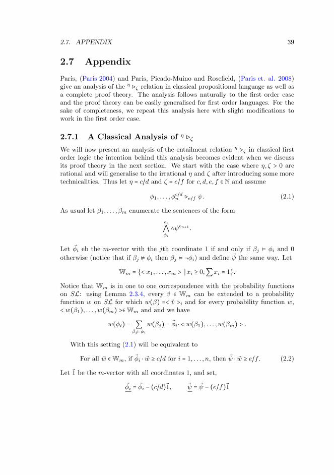
We will now present an analysis of the entailment relation η ⊳ζ in classical firstorder logic the intention behind this analysis becomes evident when we discussits proof theory in the next section. We start with the case where η, ζ > 0 arerational and will generalise to the irrational η and ζ after introducing some moretechnicalities. Thus let η = c/d and ζ = e/f for c, d, e, f ∈ N and assume
φ1, . . . , φc/dn ⊳e/f ψ. (2.1)
As usual let β1, . . . , βm enumerate the sentences of the form
εi
⋀φi
∧ψεn+1 .
Let φi eb the m-vector with the jth coordinate 1 if and only if βj ⊧ φi and 0
otherwise (notice that if βj ⊭ φi then βj ⊧ ¬φi) and define ψ the same way. Let
Wm = {< x1, . . . , xm > ∣xi ≥ 0,∑xi = 1}.
Notice that Wm is in one to one correspondence with the probability functionson SL: using Lemma 2.3.4, every v ∈ Wm can be extended to a probabilityfunction w on SL for which w(β) =< v >i and for every probability function w,< w(β1), . . . ,w(βm) >∈Wm and and we have
w(φi) = ∑βj⊧φi
w(βj) = φi⋅ < w(β1), . . . ,w(βm) > .
With this setting (2.1) will be equivalent to
For all w ∈Wm, if φi ⋅ w ≥ c/d for i = 1, . . . , n, then ψ ⋅ w ≥ e/f. (2.2)
Let 1 be the m-vector with all coordinates 1, and set,
φi = φi − (c/d)1, ψ = ψ − (e/f)1
40 CHAPTER 2. REASONING FROM CONFLICTING INFORMATION
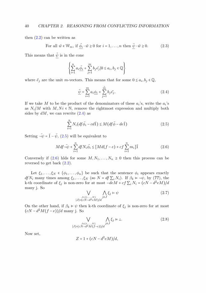
then (2.2) can be written as
For all w ∈Wm, if φi ⋅ w ≥ 0 for i = 1, . . . , n then ψ ⋅ w ≥ 0. (2.3)
This means that ψ is in the cone
⎧⎪⎪⎨⎪⎪⎩
n
∑i=1
aiφi +m
∑j=1
bj ej ∣0 ≤ ai, bj ∈ Q⎫⎪⎪⎬⎪⎪⎭
where ej are the unit m-vectors. This means that for some 0 ≤ ai, bj ∈ Q,
ψ =m
∑i=1
ai
φi +m
∑j=1
bj ej . (2.4)
If we take M to be the product of the denominators of these ai’s, write the ai’sas Ni/M with M,Ni ∈ N, remove the rightmost expression and multiply bothsides by dM , we can rewrite (2.4) as
n
∑i=1
Ni(dfφi − cd1) ≤M(dfφ − de1) (2.5)
Setting ¬ψ = 1 − ψ, (2.5) will be equivalent to
Mdf ¬ψ +n
∑i=1
dfNiφi ≤ [Md(f − e) + cfn
∑i=1
mi]1 (2.6)
Conversely if (2.6) hlds for some M,N1, . . . ,Nn ≥ 0 then this process can bereversed to get back (2.2).
Let ξ1, . . . , ξN ∈ {φ1, . . . , φn} be such that the sentence φi appears exactlydfNi many times among ξ1, . . . , ξN (so N = df ∑iNi). If βk ⊧ ¬ψ, by (??), thek-th coordinate of ξj is non-zero for at most −deM + cf ∑iNi = (cN − d2eM)/dmany j. So
⋁J⊂{1,...,N}
∣J ∣>(cN−d2eM)/d
⋀j∈J
ξj ⊧ ψ (2.7)
On the other hand, if βk ⊧ ψ then k-th coordinate of ξj is non-zero for at most(cN − d2M(f − e))/d many j. So
⋁J⊂{1,...,N}
∣J ∣>(cN−d2M(f−e))/d
⋀j∈J
ξj ⊧ �. (2.8)
Now set,Z = 1 + (cN − d2eM)/d,
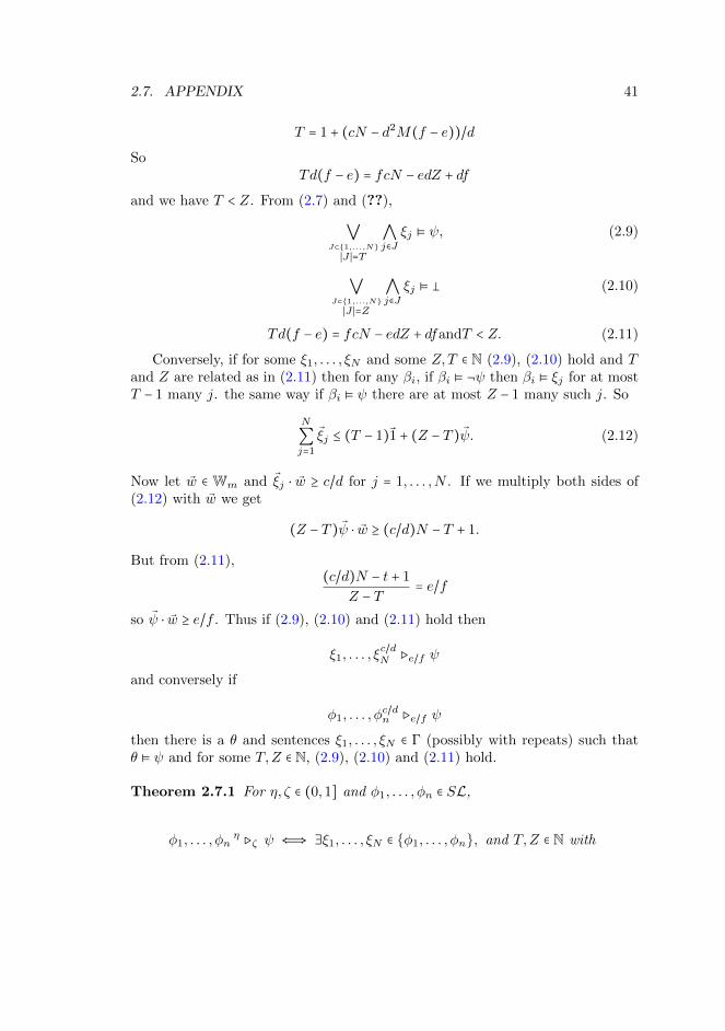
2.7. APPENDIX 41
T = 1 + (cN − d2M(f − e))/d
SoTd(f − e) = fcN − edZ + df
and we have T < Z. From (2.7) and (??),
⋁J⊂{1,...,N}∣J ∣=T
⋀j∈J
ξj ⊧ ψ, (2.9)
⋁J⊂{1,...,N}∣J ∣=Z
⋀j∈J
ξj ⊧ � (2.10)
Td(f − e) = fcN − edZ + dfandT < Z. (2.11)
Conversely, if for some ξ1, . . . , ξN and some Z,T ∈ N (2.9), (2.10) hold and Tand Z are related as in (2.11) then for any βi, if βi ⊧ ¬ψ then βi ⊧ ξj for at mostT − 1 many j. the same way if βi ⊧ ψ there are at most Z − 1 many such j. So
N
∑j=1
ξj ≤ (T − 1)1 + (Z − T )ψ. (2.12)
Now let w ∈ Wm and ξj ⋅ w ≥ c/d for j = 1, . . . ,N . If we multiply both sides of(2.12) with w we get
(Z − T )ψ ⋅ w ≥ (c/d)N − T + 1.
But from (2.11),(c/d)N − t + 1
Z − T= e/f
so ψ ⋅ w ≥ e/f . Thus if (2.9), (2.10) and (2.11) hold then
ξ1, . . . , ξc/dN ⊳e/f ψ
and conversely if
φ1, . . . , φc/dn ⊳e/f ψ
then there is a θ and sentences ξ1, . . . , ξN ∈ Γ (possibly with repeats) such thatθ ⊧ ψ and for some T,Z ∈ N, (2.9), (2.10) and (2.11) hold.
Theorem 2.7.1 For η, ζ ∈ (0,1] and φ1, . . . , φn ∈ SL,
φ1, . . . , φnη ⊳ζ ψ ⇐⇒ ∃ξ1, . . . , ξN ∈ {φ1, . . . , φn}, and T,Z ∈ N with
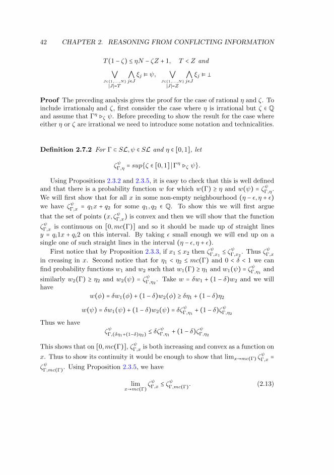
42 CHAPTER 2. REASONING FROM CONFLICTING INFORMATION
T (1 − ζ) ≤ ηN − ζZ + 1, T < Z and
⋁J⊂{1,...,N}∣J ∣=T
⋀j∈J
ξj ⊧ ψ, ⋁J⊂{1,...,N}∣J ∣=Z
⋀j∈J
ξj ⊧ �
Proof The preceding analysis gives the proof for the case of rational η and ζ. Toinclude irrationalη and ζ, first consider the case where η is irrational but ζ ∈ Qand assume that Γη ⊳ζ ψ. Before preceding to show the result for the case whereeither η or ζ are irrational we need to introduce some notation and technicalities.
Definition 2.7.2 For Γ ⊂ SL, ψ ∈ SL and η ∈ [0,1], let
ζψΓ,η = sup{ζ ∈ [0,1] ∣Γη ⊳ζ ψ}.
Using Propositions 2.3.2 and 2.3.5, it is easy to check that this is well definedand that there is a probability function w for which w(Γ) ≥ η and w(ψ) = ζψΓ,η.
We will first show that for all x in some non-empty neighbourhood (η − ε, η + ε)
we have ζψΓ,x = q1x + q2 for some q1, q2 ∈ Q. To show this we will first argue
that the set of points (x, ζψΓ,x) is convex and then we will show that the function
ζψΓ,x is continuous on [0,mc(Γ)] and so it should be made up of straight linesy = qi1x + qi2 on this interval. By taking ε small enough we will end up on asingle one of such straight lines in the interval (η − ε, η + ε).
First notice that by Proposition 2.3.3, if x1 ≤ x2 then ζψΓ,x1≤ ζψΓ,x2
. Thus ζψΓ,xin creasing in x. Second notice that for η1 < η2 ≤ mc(Γ) and 0 < δ < 1 we can
find probability functions w1 and w2 such that w1(Γ) ≥ η1 and w1(ψ) = ζψΓ,η1
and
similarly w2(Γ) ≥ η2 and w2(ψ) = ζψΓ,η2
. Take w = δw1 + (1 − δ)w2 and we willhave
w(φ) = δw1(φ) + (1 − δ)w2(φ) ≥ δη1 + (1 − δ)η2
w(ψ) = δw1(ψ) + (1 − δ)w2(ψ) = δζψΓ,η1
+ (1 − δ)ζψΓ,η2
Thus we have
ζψΓ,(δη1+(1−δ)η2) ≤ δζ
ψΓ,η1
+ (1 − δ)ζψΓ,η2
This shows that on [0,mc(Γ)], ζψΓ,x is both increasing and convex as a function on
x. Thus to show its continuity it would be enough to show that limx→mc(Γ) ζψΓ,x =
ζψΓ,mc(Γ). Using Proposition 2.3.5, we have
limx→mc(Γ)
ζψΓ,x ≤ ζψΓ,mc(Γ). (2.13)
2.7. APPENDIX 43
If limx→mc(Γ) ζψΓ,x < ζ
ψΓ,mc(Γ) then we can take
limx→mc(Γ)
ζψΓ, < t < ζψΓ,mc(Γ)
we can then find an increasing sequence rn converging to mc(Γ) and probabilityfunctions wn for which wn(Γ) ≥ rn and wn(ψ) < t. For Γ = {φ1, . . . , φn} and asusual let βi, i = 1, . . . ,m enumerate the sentences
n
⋀i
φεii ∧ ψεn+1
and consider the vector
wj =< wj(β1), . . . ,wj(βm) > .
Since wj(β1) is a bounded sequence it has a convergent subsequence, say w1j(β1),converging to say, w(β1). Let
w1j =< w
1j (β1), . . . ,w
1j (βm) >
be a subsequence of wj such that w1j is a subsequence of w1j (so w1
j (β1) converges
to w(β1) ). The same way we have wj1(β2) is a bounded sequence and so has aconvergent subsequence, say w2j(β2), converging to say w(β2) and let
w2j =< w
2j (β1), . . . ,w
2j (βm) >
be a subsequence of w1j for which w2
j (β2) is a subsequence of w2j(β2) and so con-verges to w(β2). By the same method we will eventually construct a convergentsubsequence of wj , namely wmj , that converges to
w =< w(β1), . . . ,w(βm) > .
Using Lemma 2.3.4 we can extend this to a probability function w on SL and forall φ ∈ Γ
w(φ) = ∑βk⊧φ
w(βk) = ∑βk⊧φ
limj→∞
wmj (βk) = limj→∞
∑βk⊧φ
wj(βk) = limj→∞
wj(φ) ≥ limj→∞
rj = r
while
w(ψ) = ∑βk⊧ψ
w(βk) = ∑βk⊧ψ
limj→∞
wmj (βk)
= limj→∞
∑βk⊧ψ
wj(βk) = limj→∞
wj(ψ) < limj→∞
t = t < ζψΓ,mc(Γ)
44 CHAPTER 2. REASONING FROM CONFLICTING INFORMATION
which is a contradiction. Thus the strict inequality can hold in (2.13) and wehave
limx→mc(Γ)
ζψΓ,x = ζψΓ,mc(Γ)
as required. It only remains to show that the set of pints (x, ζψΓ,x) is convex. Take
Ψ(x, y) to be a formula in the language R =< R,+,≤,0,1 > such that for η, ζ ∈
[0,1], R ⊧ Ψ(η, ζ) ⇐⇒ ζψΓ,η = ζ. Then since R admits quantifier elimination and
is an elementary extension of Q =< Q,+,≤,0,1 > we can suppose that Ψ(x, y) isof the form
s
⋁i=1
us
⋀j=1
(mijy ∗ nijx + kij)
for some mij , nij , kij ∈ Z, where ∗ is either < or ≤. The set of pairs (x, y) for
which R ⊧ ⋀usj=1(mijy ∗ nijx + kij) is convex. Since ζψΓ,x is a continuous and
convex function of x it must be a straight line y = qi1x + qi2 with coefficientsqi1, qi2 ∈ Q with x ranging over some proper interval (which we can take to be
closed since ζψΓ,x is continuous).Returning to our proof of Theorem 2.7.1, take η irrational and ζ rational and
assumeφ1, . . . , φn
η ⊳ζ ψ,
By the discussion above, ζψΓ,x = q1x + q2 for all x in some non-empty interval
(η − ε, η + ε). Since q1η + q2 is irrational we should have q1η + q2 > ζ (notice
that ζψΓ,x = q1x + q2 is the maximum on all zeta for which φ1, . . . , φnη ⊳ζ ψ
and the equlity cannot hold) so there are r1, r2 ∈ Q such that r1 < η, r2 > ζ
and q1r1 + q2 > r2. Taking r1 withing the ε of η then ζψΓ,x > r2 so from thefirst case for rational thresholds we can find ξ1, . . . , ξN ∈ Γ and Z,T such thatT (1 − r2) ≤ r1N − r2Z + 1, T < Z
⋁J⊂{1,...,N}∣J ∣=T
⋀j∈J
ξj ⊧ ψ, ⋁J⊂{1,...,N}∣J ∣=Z
⋀j∈J
ξj ⊧ � (2.14)
and by taking r1 and r2 close enough to η and ζ we will have
T (1 − ζ) ≤ ηN − ζZ + 1 (2.15)
as required by Theorem 2.7.1. Conversely if we have ξ1, . . . , ξN ∈ Γ and Z,Tsatisfying (2.14) and (2.15), there must be r1 < η and r2 > ζ such that
T (1 − r2) ≤ r1N − r2Z + 1
and by the rational case above we should have φ1, . . . , φnr1 ⊳r2 ψ and thus by
Proposition 2.3.3 we haveφ1, . . . , φn
η ⊳ζ ψ.
2.7. APPENDIX 45
The third case where η ∈ Q and ζ ∉ Q is proved similarly. For the last casewhere η, ζ are both irrational assume Γη ⊳ζ ψ. First notice that if ζψΓ,x > ζ thenwe can take a rational r2 > ζ and close enough to ζ and proceed as above so wewill assume that ζψΓ,x = q1η + q2 = ζ. The by the discussion above we have that
ζψΓ,x = q1η+q2 in some non-empty interval (η+ε, η−ε), and we can choose r1 ∈ Q inthis interval and set r2 = q1r1 + q2 and by the first case for rational thresholds wehave ξ1, . . . , ξN ∈ Γ and Z < T with T (1 − r2) ≤ r1N − r2Z + 1. We notice that weshould have equality here otherwise we could increase r2 while keeping r1 fixedand show that ζψΓ,r1 > r2 which contradicts the choice of r2. These Z and T work
for r1 arbitrarily close to η (and r2 = q1r1+q2) and so by taking the limit one canreadily check that the same Z and T will satisfy the required inequality also forη and ζ. In the other direction, suppose we have ξ1, . . . ξN for which (2.13) holdand Z,T that satisfy the required inequalities. Then for rational r1 close to η
and r2 ≤(r1N−T+1)(Z−T ) close to ζ these same ξ1, . . . , ξN , Z and T will give Γr1 ⊳r2 ψ.
Since r1 and r2 can be made arbitrarily close to η and ζ respectively we can useProposition 2.3.5 to get Γη ⊳ζ ψ.

46 CHAPTER 2. REASONING FROM CONFLICTING INFORMATION
Chapter 3
Learning IndicativeConditionals
3.1 Introduction
Indicative conditional statements of the form “if A, then B” constitute a substan-tial part of the evidence that we obtain. But how should we change our beliefs inthe light of such evidence? This question has prompted a large literature. How-ever, in a recent survey, (Douven 2012) concludes that a proper general accountof probabilistic belief updating by learning (probabilistic) conditional informationis still to be formulated. And indeed, all accounts that have been proposed so farhave problems. Here are three of them. (For a much more detailed discussion,see (Douven 2012).)
First and most straightforwardly, one might identify the natural lan-guage indicative conditional A → B with the material conditional A ⊃ B,which is equivalent to ¬A ∨ B. In a well-known article, Popper and Miller,(Popper & Miller 1983), challenged this proposal with an argument based onthe probability calculus. It goes as follows. Consider two propositions A and Band a prior probability distribution P with 0 < P (A) < 1 and P (B∣A) < 1. Wenow learn the indicative conditional A → B, which we express as the materialconditional A ⊃ B. To update our beliefs, we use Bayesian Conditionalisation,i.e. we calculate the posterior probability P ∗(A) ∶= P (A∣¬A ∨B). Interestingly,it turns out that P ∗(A) < P (A). That is, learning that B follows from A alwaysdecreases the probability of A if one uses the material conditional. However,there are examples (such as the Sundowners Example discussed below) wherethe posterior probability is intuitively judged to be greater than or equal to the
47
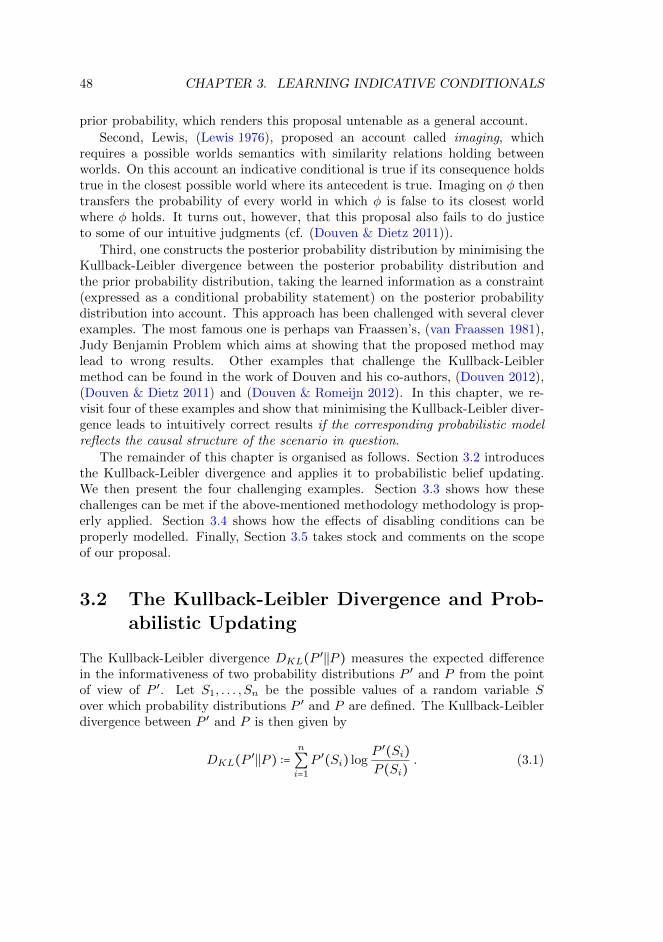
48 CHAPTER 3. LEARNING INDICATIVE CONDITIONALS
prior probability, which renders this proposal untenable as a general account.
Second, Lewis, (Lewis 1976), proposed an account called imaging, whichrequires a possible worlds semantics with similarity relations holding betweenworlds. On this account an indicative conditional is true if its consequence holdstrue in the closest possible world where its antecedent is true. Imaging on φ thentransfers the probability of every world in which φ is false to its closest worldwhere φ holds. It turns out, however, that this proposal also fails to do justiceto some of our intuitive judgments (cf. (Douven & Dietz 2011)).
Third, one constructs the posterior probability distribution by minimising theKullback-Leibler divergence between the posterior probability distribution andthe prior probability distribution, taking the learned information as a constraint(expressed as a conditional probability statement) on the posterior probabilitydistribution into account. This approach has been challenged with several cleverexamples. The most famous one is perhaps van Fraassen’s, (van Fraassen 1981),Judy Benjamin Problem which aims at showing that the proposed method maylead to wrong results. Other examples that challenge the Kullback-Leiblermethod can be found in the work of Douven and his co-authors, (Douven 2012),(Douven & Dietz 2011) and (Douven & Romeijn 2012). In this chapter, we re-visit four of these examples and show that minimising the Kullback-Leibler diver-gence leads to intuitively correct results if the corresponding probabilistic modelreflects the causal structure of the scenario in question.
The remainder of this chapter is organised as follows. Section 3.2 introducesthe Kullback-Leibler divergence and applies it to probabilistic belief updating.We then present the four challenging examples. Section 3.3 shows how thesechallenges can be met if the above-mentioned methodology methodology is prop-erly applied. Section 3.4 shows how the effects of disabling conditions can beproperly modelled. Finally, Section 3.5 takes stock and comments on the scopeof our proposal.
3.2 The Kullback-Leibler Divergence and Prob-abilistic Updating
The Kullback-Leibler divergence DKL(P′∣∣P ) measures the expected difference
in the informativeness of two probability distributions P ′ and P from the pointof view of P ′. Let S1, . . . , Sn be the possible values of a random variable Sover which probability distributions P ′ and P are defined. The Kullback-Leiblerdivergence between P ′ and P is then given by
DKL(P′∣∣P ) ∶=
n
∑i=1
P ′(Si) logP ′(Si)
P (Si). (3.1)
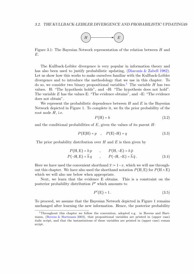
3.2. THE KULLBACK-LEIBLER DIVERGENCE AND PROBABILISTIC UPDATING49
H E
Figure 3.1: The Bayesian Network representation of the relation between H andE.
The Kullback-Leibler divergence is very popular in information theory andhas also been used to justify probabilistic updating, (Diaconis & Zabell 1982).Let us show how this works to make ourselves familiar with the Kullback-Leiblerdivergence and to introduce the methodology that we use in this chapter. Todo so, we consider two binary propositional variables.1 The variable H has twovalues. H: “The hypothesis holds”, and ¬H: “The hypothesis does not hold”.The variable E has the values E: “The evidence obtains”, and ¬E: “The evidencedoes not obtain”.
We represent the probabilistic dependence between H and E in the BayesianNetwork depicted in Figure 1. To complete it, we fix the prior probability of theroot node H, i.e.
P (H) = h (3.2)
and the conditional probabilities of E, given the values of its parent H:
P (E∣H) = p , P (E∣¬H) = q (3.3)
The prior probability distribution over H and E is then given by
P (H,E) = hp , P (H,¬E) = hp
P (¬H,E) = hq , P (¬H,¬E) = hq . (3.4)
Here we have used the convenient shorthand x ∶= 1−x, which we will use through-out this chapter. We have also used the shorthand notation P (H,E) for P (H ∧E)which we will also use below when appropriate.
Next, we learn that the evidence E obtains. This is a constraint on theposterior probability distribution P ′ which amounts to
P ′(E) = 1 . (3.5)
To proceed, we assume that the Bayesian Network depicted in Figure 1 remainsunchanged after learning the new information. Hence, the posterior probability
1Throughout this chapter we follow the convention, adopted e.g. in Bovens and Hart-mann, (Bovens & Hartmann 2003), that propositional variables are printed in (upper case)italic script, and that the instantiations of these variables are printed in (upper case) romanscript.
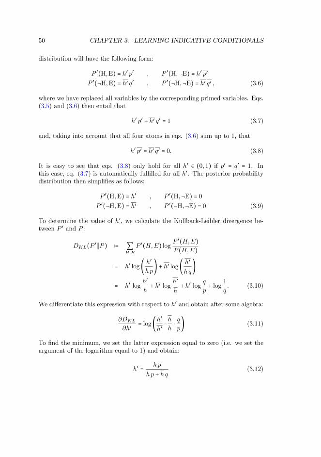
50 CHAPTER 3. LEARNING INDICATIVE CONDITIONALS
distribution will have the following form:
P ′(H,E) = h′ p′ , P ′(H,¬E) = h′ p′
P ′(¬H,E) = h′ q′ , P ′(¬H,¬E) = h′ q′ , (3.6)
where we have replaced all variables by the corresponding primed variables. Eqs.(3.5) and (3.6) then entail that
h′ p′ + h′ q′ = 1 (3.7)
and, taking into account that all four atoms in eqs. (3.6) sum up to 1, that
h′ p′ = h′ q′ = 0. (3.8)
It is easy to see that eqs. (3.8) only hold for all h′ ∈ (0,1) if p′ = q′ = 1. Inthis case, eq. (3.7) is automatically fulfilled for all h′. The posterior probabilitydistribution then simplifies as follows:
P ′(H,E) = h′ , P ′(H,¬E) = 0
P ′(¬H,E) = h′ , P ′(¬H,¬E) = 0 (3.9)
To determine the value of h′, we calculate the Kullback-Leibler divergence be-tween P ′ and P :
DKL(P′∣∣P ) ∶= ∑
H,E
P ′(H,E) logP ′(H,E)
P (H,E)
= h′ log(h′
hp) + h′ log(
h′
hq)
= h′ logh′
h+ h′ log
h′
h+ h′ log
q
p+ log
1
q. (3.10)
We differentiate this expression with respect to h′ and obtain after some algebra:
∂DKL
∂h′= log(
h′
h′⋅h
h⋅q
p) (3.11)
To find the minimum, we set the latter expression equal to zero (i.e. we set theargument of the logarithm equal to 1) and obtain:
h′ =hp
hp + hq(3.12)
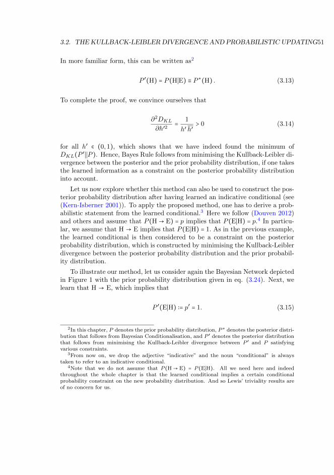
3.2. THE KULLBACK-LEIBLER DIVERGENCE AND PROBABILISTIC UPDATING51
In more familiar form, this can be written as2
P ′(H) = P (H∣E) ≡ P ∗(H) . (3.13)
To complete the proof, we convince ourselves that
∂2DKL
∂h′2=
1
h′ h′> 0 (3.14)
for all h′ ∈ (0,1), which shows that we have indeed found the minimum ofDKL(P
′∣∣P ). Hence, Bayes Rule follows from minimising the Kullback-Leibler di-vergence between the posterior and the prior probability distribution, if one takesthe learned information as a constraint on the posterior probability distributioninto account.
Let us now explore whether this method can also be used to construct the pos-terior probability distribution after having learned an indicative conditional (see(Kern-Isberner 2001)). To apply the proposed method, one has to derive a prob-abilistic statement from the learned conditional.3 Here we follow (Douven 2012)and others and assume that P (H→ E) = p implies that P (E∣H) = p.4 In particu-lar, we assume that H → E implies that P (E∣H) = 1. As in the previous example,the learned conditional is then considered to be a constraint on the posteriorprobability distribution, which is constructed by minimising the Kullback-Leiblerdivergence between the posterior probability distribution and the prior probabil-ity distribution.
To illustrate our method, let us consider again the Bayesian Network depictedin Figure 1 with the prior probability distribution given in eq. (3.24). Next, welearn that H → E, which implies that
P ′(E∣H) ∶= p′ = 1. (3.15)
2In this chapter, P denotes the prior probability distribution, P ∗ denotes the posterior distri-bution that follows from Bayesian Conditionalisation, and P ′ denotes the posterior distributionthat follows from minimising the Kullback-Leibler divergence between P ′ and P satisfyingvarious constraints.
3From now on, we drop the adjective “indicative” and the noun “conditional” is alwaystaken to refer to an indicative conditional.
4Note that we do not assume that P (H→ E) = P (E∣H). All we need here and indeedthroughout the whole chapter is that the learned conditional implies a certain conditionalprobability constraint on the new probability distribution. And so Lewis’ triviality results areof no concern for us.
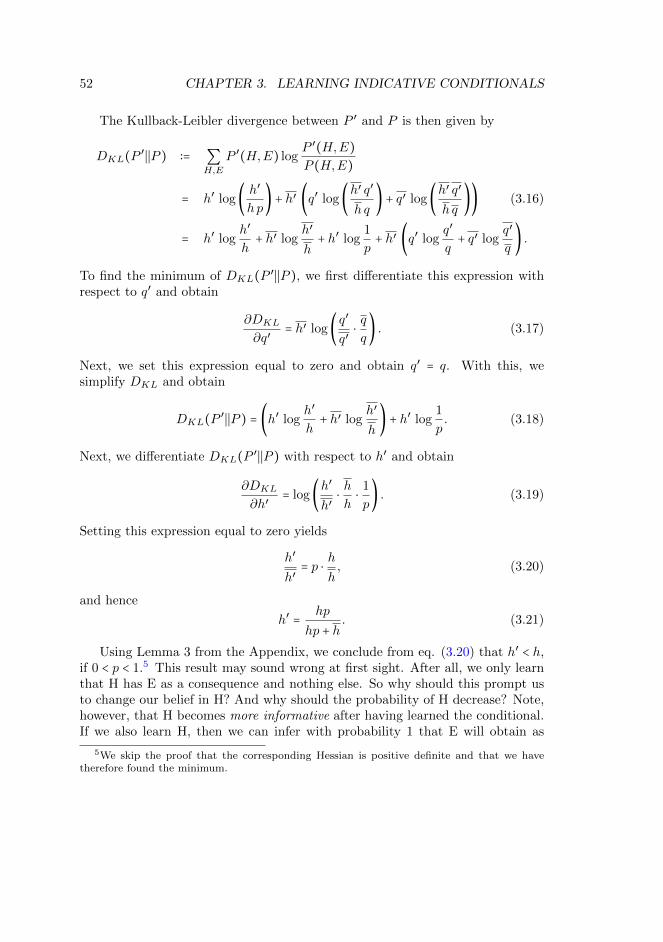
52 CHAPTER 3. LEARNING INDICATIVE CONDITIONALS
The Kullback-Leibler divergence between P ′ and P is then given by
DKL(P′∣∣P ) ∶= ∑
H,E
P ′(H,E) logP ′(H,E)
P (H,E)
= h′ log(h′
hp) + h′ (q′ log(
h′ q′
hq) + q′ log(
h′ q′
hq)) (3.16)
= h′ logh′
h+ h′ log
h′
h+ h′ log
1
p+ h′ (q′ log
q′
q+ q′ log
q′
q) .
To find the minimum of DKL(P′∣∣P ), we first differentiate this expression with
respect to q′ and obtain
∂DKL
∂q′= h′ log(
q′
q′⋅q
q) . (3.17)
Next, we set this expression equal to zero and obtain q′ = q. With this, wesimplify DKL and obtain
DKL(P′∣∣P ) = (h′ log
h′
h+ h′ log
h′
h) + h′ log
1
p. (3.18)
Next, we differentiate DKL(P′∣∣P ) with respect to h′ and obtain
∂DKL
∂h′= log(
h′
h′⋅h
h⋅1
p) . (3.19)
Setting this expression equal to zero yields
h′
h′= p ⋅
h
h, (3.20)
and hence
h′ =hp
hp + h. (3.21)
Using Lemma 3 from the Appendix, we conclude from eq. (3.20) that h′ < h,if 0 < p < 1.5 This result may sound wrong at first sight. After all, we only learnthat H has E as a consequence and nothing else. So why should this prompt usto change our belief in H? And why should the probability of H decrease? Note,however, that H becomes more informative after having learned the conditional.If we also learn H, then we can infer with probability 1 that E will obtain as
5We skip the proof that the corresponding Hessian is positive definite and that we havetherefore found the minimum.
3.2. THE KULLBACK-LEIBLER DIVERGENCE AND PROBABILISTIC UPDATING53
well. It is therefore natural to set the new probability of H to a lower valueas more informative hypotheses have a lower probability than less informativehypotheses.6
We have seen that minimising the Kulback-Leibler divergence leads to reason-able results for situations involving two propositional variables. But does it alsowork for more complicated scenarios? Douven and van Fraassen do not think so,and here are four of their alleged counterexamples. Each example starts with astory that sets up the scene. Then a conditional is learned which may promptsome previously held beliefs to change.
1. The Sundowners Example. Sarah and her sister Marian have arranged togo for sundowners at the Westcliff hotel tomorrow. Sarah feels that thereis some chance that it will rain, but thinks they can always enjoy the viewfrom inside. To make sure, Marian consults the staff at the Westcliff hoteland finds out that in the event of rain, the inside area will be occupied bya wedding party. So she tells Sarah: “If it rains tomorrow, then we cannothave sundowners at the Westcliff.” Upon learning this conditional, Sarahsets her probability for sundowners and rain to 0, but does not change herprobability for rain. Thus, in this example, learning the conditional infor-mation has the effect of leaving the probability of the antecedent unchanged.This example is from (Douven & Romeijn 2012).
2. The Ski Trip Example. Harry sees his friend Sue buying a ski outfit. Thissurprises him a bit, because he did not know of any plans of hers to go ona ski trip. He knows that she recently had an important exam and thinksit unlikely that she passed it. Then he meets Tom, his best friend and alsoa friend of Sue’s, who is just on his way to Sue to hear whether she passedthe exam, and who tells him: “If Sue passed the exam, her father willtake her on a ski vacation.” Recalling his earlier observation, Harry nowcomes to find it more likely that Sue passed the exam. So in this exampleupon learning the conditional information Harry should intuitively increasethe probability of the antecedent of the conditional. This example is from(Douven & Dietz 2011).
3. The Driving Test Example. Betty knows that Kevin, the son of her neigh-bours, was to take his driving test yesterday. She has no idea whether or
6Note that eq. (3.21) also obtains if one learns the material conditional H ⊃ E ≡ ¬H ∨E anduses Bayesian Conditionalisation to update one’s beliefs:
P ∗(H) = P (H∣¬H ∨E) =P (H ∧ (¬H ∨E))
P (¬H ∨E)=
P (H,E)
P (H,E) + P (¬H)
=hp
hp + h≡ h′
54 CHAPTER 3. LEARNING INDICATIVE CONDITIONALS
not Kevin is a good driver; she deems it about as likely as not that Kevinpassed the test. Betty notices that her neighbours have started to spadetheir garden. Then her mother, who is friends with Kevin’s parents, callsher and tells her the following: “If Kevin passed the driving test, his parentswill throw a garden party.” Betty figures that, given the spading that hasjust begun, it is doubtful (even if not wholly excluded) that a party can beheld in the garden of Kevin’s parents in the near future. As a result, Bettylowers her degree of belief for Kevin’s having passed the driving test andthus decreases the probability of the antecedent of the conditional. Thisexample is from (Douven 2012).
While the first three examples are meant to be challenges to the Kullback-Leibler method, the following problem is an alleged counterexample.
4. The Judy Benjamin Problem. A soldier, Judy Benjamin, is dropped withher platoon in a territory that is divided in two halves, Red territory andBlue territory, respectively, with each territory in turn being divided inequal parts, Second Company area and Headquarters Company area, thusforming four quadrants of roughly equal size. Because the platoon wasdropped more or less at the centre of the whole territory, Judy Benjamindeems it equally likely that they are in one quadrant as that they are inany of the others. They then receive the following radio message: “I can’tbe sure where you are. If you are in Red Territory, then the odds are 3 ∶ 1that you are in Second Company area.” After this, the radio contact breaksdown. Supposing that Judy accepts this message, how should she adjusther degrees of belief?7
To address this question, we introduce two binary propositional variables.The variable R has the values R: “Judy lands in Red Territory”, and ¬R: “Judylands in Blue Territory”. The variable S has the values S: “Judy lands in SecondCompany”, and ¬S: “Judy lands in Headquarters”. The probabilistic dependencebetween R and S is depicted in the Bayesian Network in Figure 2. To completeit, we fix the prior probability of the root node R, i.e.
P (R) = r (3.22)
and the conditional probabilities of S, given the values of its parent R:
P (S∣R) = p , P (S∣¬R) = q (3.23)
7This example is from (van Fraassen 1981).
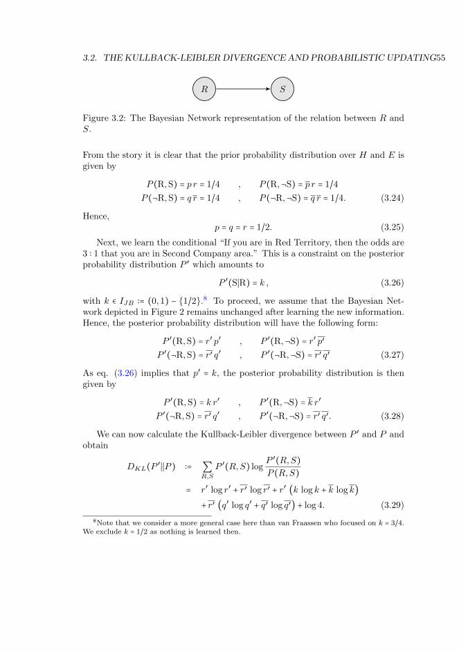
3.2. THE KULLBACK-LEIBLER DIVERGENCE AND PROBABILISTIC UPDATING55
R S
Figure 3.2: The Bayesian Network representation of the relation between R andS.
From the story it is clear that the prior probability distribution over H and E isgiven by
P (R,S) = p r = 1/4 , P (R,¬S) = p r = 1/4
P (¬R,S) = q r = 1/4 , P (¬R,¬S) = q r = 1/4. (3.24)
Hence,p = q = r = 1/2. (3.25)
Next, we learn the conditional “If you are in Red Territory, then the odds are3 ∶ 1 that you are in Second Company area.” This is a constraint on the posteriorprobability distribution P ′ which amounts to
P ′(S∣R) = k , (3.26)
with k ∈ IJB ∶= (0,1) − {1/2}.8 To proceed, we assume that the Bayesian Net-work depicted in Figure 2 remains unchanged after learning the new information.Hence, the posterior probability distribution will have the following form:
P ′(R,S) = r′ p′ , P ′(R,¬S) = r′ p′
P ′(¬R,S) = r′ q′ , P ′(¬R,¬S) = r′ q′ (3.27)
As eq. (3.26) implies that p′ = k, the posterior probability distribution is thengiven by
P ′(R,S) = k r′ , P ′(R,¬S) = k r′
P ′(¬R,S) = r′ q′ , P ′(¬R,¬S) = r′ q′. (3.28)
We can now calculate the Kullback-Leibler divergence between P ′ and P andobtain
DKL(P′∣∣P ) ∶= ∑
R,S
P ′(R,S) logP ′(R,S)
P (R,S)
= r′ log r′ + r′ log r′ + r′ (k log k + k log k)
+ r′ (q′ log q′ + q′ log q′) + log 4. (3.29)
8Note that we consider a more general case here than van Fraassen who focused on k = 3/4.We exclude k = 1/2 as nothing is learned then.
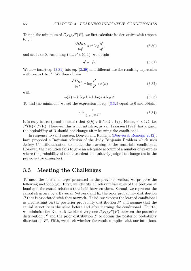
56 CHAPTER 3. LEARNING INDICATIVE CONDITIONALS
To find the minimum of DKL(P′∣∣P ), we first calculate its derivative with respect
to q′,∂DKL
∂q′= r′ log
q′
q′, (3.30)
and set it to 0. Assuming that r′ ∈ (0,1), we obtain
q′ = 1/2. (3.31)
We now insert eq. (3.31) into eq. (3.29) and differentiate the resulting expressionwith respect to r′. We then obtain
∂DKL
∂r′= log
r′
r′+ φ(k) (3.32)
withφ(k) ∶= k log k + k log k + log 2 . (3.33)
To find the minimum, we set the expression in eq. (3.32) equal to 0 and obtain
r′ =1
1 + eφ(k). (3.34)
It is easy to see (proof omitted) that φ(k) > 0 for k ∈ IJB . Hence, r′ < 1/2, i.e.P ′(R) < P (R). However, this is not intuitive, as van Fraassen (1981) has argued:the probability of R should not change after learning the conditional.
In response to van Fraassen, Douven and Romeijn (Douven & Romeijn 2012),have proposed a Bayesian solution of the Judy Benjamin Problem which usesJeffrey Conditionalisation to model the learning of the uncertain conditional.However, their solution fails to give an adequate account of a number of exampleswhere the probability of the antecedent is intuitively judged to change (as in theprevious two examples).
3.3 Meeting the Challenges
To meet the four challenges presented in the previous section, we propose thefollowing methodology. First, we identify all relevant variables of the problem athand and the causal relations that hold between them. Second, we represent thecausal structure by a Bayesian Network and fix the prior probability distributionP that is associated with that network. Third, we express the learned conditionalas a constraint on the posterior probability distribution P ′ and assume that thecausal structure is the same before and after learning the conditional. Fourth,we minimise the Kullback-Leibler divergence DKL(P
′∣∣P ) between the posteriordistribution P ′ and the prior distribution P to obtain the posterior probabilitydistribution P ′. Fifth, we check whether the result complies with our intuitions.
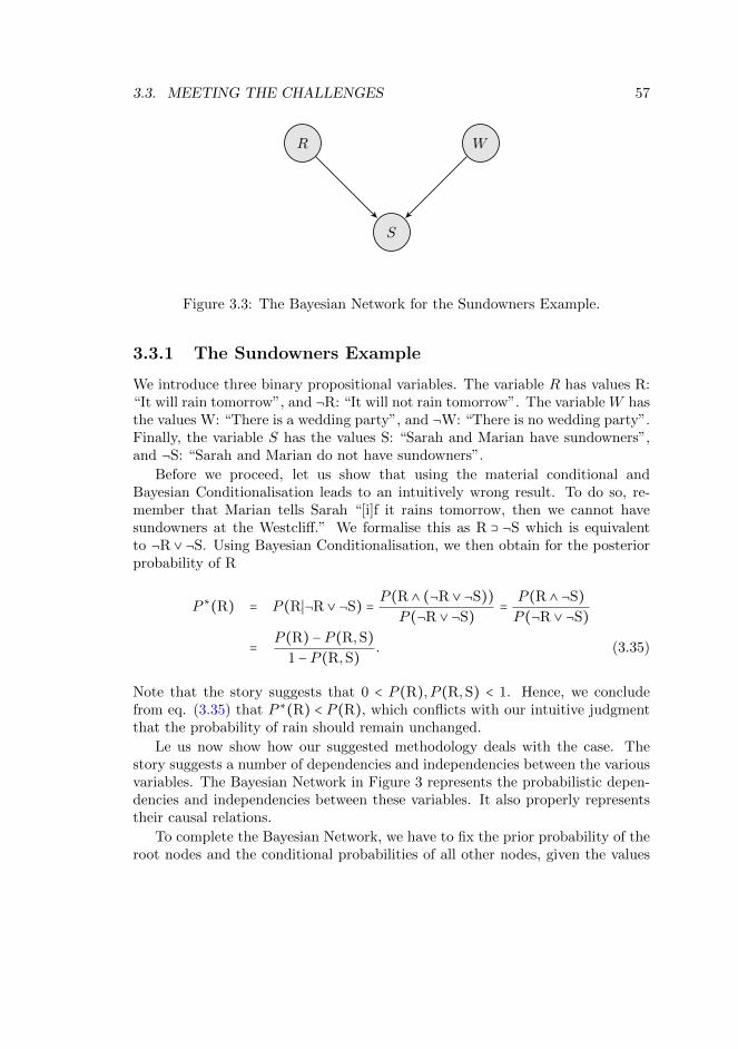
3.3. MEETING THE CHALLENGES 57
R
S
W
Figure 3.3: The Bayesian Network for the Sundowners Example.
3.3.1 The Sundowners Example
We introduce three binary propositional variables. The variable R has values R:“It will rain tomorrow”, and ¬R: “It will not rain tomorrow”. The variable W hasthe values W: “There is a wedding party”, and ¬W: “There is no wedding party”.Finally, the variable S has the values S: “Sarah and Marian have sundowners”,and ¬S: “Sarah and Marian do not have sundowners”.
Before we proceed, let us show that using the material conditional andBayesian Conditionalisation leads to an intuitively wrong result. To do so, re-member that Marian tells Sarah “[i]f it rains tomorrow, then we cannot havesundowners at the Westcliff.” We formalise this as R ⊃ ¬S which is equivalentto ¬R ∨ ¬S. Using Bayesian Conditionalisation, we then obtain for the posteriorprobability of R
P ∗(R) = P (R∣¬R ∨ ¬S) =P (R ∧ (¬R ∨ ¬S))
P (¬R ∨ ¬S)=P (R ∧ ¬S)
P (¬R ∨ ¬S)
=P (R) − P (R,S)
1 − P (R,S). (3.35)
Note that the story suggests that 0 < P (R), P (R,S) < 1. Hence, we concludefrom eq. (3.35) that P ∗(R) < P (R), which conflicts with our intuitive judgmentthat the probability of rain should remain unchanged.
Le us now show how our suggested methodology deals with the case. Thestory suggests a number of dependencies and independencies between the variousvariables. The Bayesian Network in Figure 3 represents the probabilistic depen-dencies and independencies between these variables. It also properly representstheir causal relations.
To complete the Bayesian Network, we have to fix the prior probability of theroot nodes and the conditional probabilities of all other nodes, given the values
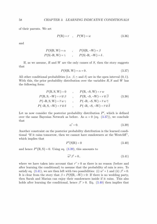
58 CHAPTER 3. LEARNING INDICATIVE CONDITIONALS
of their parents. We set
P (R) = r , P (W) = w (3.36)
and
P (S∣R,W) = α , P (S∣R,¬W) = β
P (S∣¬R,W) = γ , P (S∣¬R,¬W) = δ .
If, as we assume, R and W are the only causes of S, then the story suggeststhat
P (S∣R,W) = α = 0 . (3.37)
All other conditional probabilities (i.e. β, γ and δ) are in the open interval (0,1).With this, the prior probability distribution over the variables R,S and W hasthe following form:
P (R,S,W) = 0 , P (R,¬S,W) = r w
P (R,S,¬W) = r w β , P (R,¬S,¬W) = r w β (3.38)
P (¬R,S,W) = r w γ , P (¬R,¬S,W) = r w γ
P (¬R,S,¬W) = r w δ , P (¬R,¬S,¬W) = r w δ
Let us now consider the posterior probability distribution P ′, which is definedover the same Bayesian Network as before. As α = 0 (eq. (3.37)), we concludethat
α′ = 0. (3.39)
Another constraint on the posterior probability distribution is the learned condi-tional “If it rains tomorrow, then we cannot have sundowners at the Westcliff”,which implies that
P ′(S∣R) = 0 (3.40)
and hence P ′(R,S) = 0. Using eq. (3.39), this amounts to
w′ β′ = 0 , (3.41)
where we have taken into account that r′ > 0 as there is no reason (before andafter learning the conditional) to assume that the probability of rain is zero. Tosatisfy eq. (3.41), we are then left with two possibilities: (i) w′ = 1 and (ii) β′ = 0.It is clear from the story that β = P (S∣R,¬W) > 0: If there is no wedding party,then Sarah and Marian can enjoy their sundowners inside if it rains. This alsoholds after learning the conditional, hence β′ > 0. Eq. (3.40) then implies that
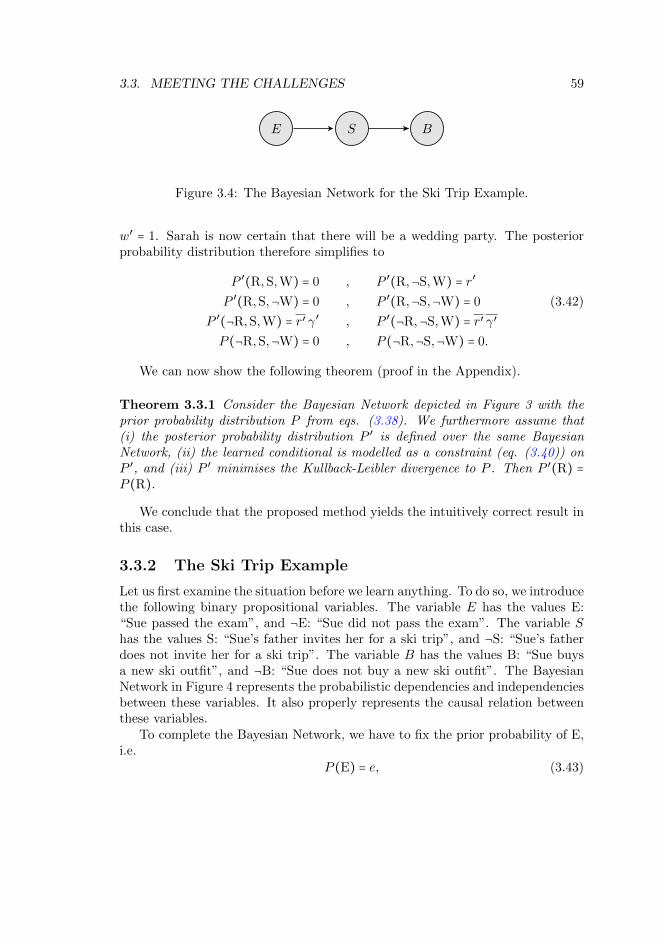
3.3. MEETING THE CHALLENGES 59
E S B
Figure 3.4: The Bayesian Network for the Ski Trip Example.
w′ = 1. Sarah is now certain that there will be a wedding party. The posteriorprobability distribution therefore simplifies to
P ′(R,S,W) = 0 , P ′(R,¬S,W) = r′
P ′(R,S,¬W) = 0 , P ′(R,¬S,¬W) = 0 (3.42)
P ′(¬R,S,W) = r′ γ′ , P ′(¬R,¬S,W) = r′ γ′
P (¬R,S,¬W) = 0 , P (¬R,¬S,¬W) = 0.
We can now show the following theorem (proof in the Appendix).
Theorem 3.3.1 Consider the Bayesian Network depicted in Figure 3 with theprior probability distribution P from eqs. (3.38). We furthermore assume that(i) the posterior probability distribution P ′ is defined over the same BayesianNetwork, (ii) the learned conditional is modelled as a constraint (eq. (3.40)) onP ′, and (iii) P ′ minimises the Kullback-Leibler divergence to P . Then P ′(R) =P (R).
We conclude that the proposed method yields the intuitively correct result inthis case.
3.3.2 The Ski Trip Example
Let us first examine the situation before we learn anything. To do so, we introducethe following binary propositional variables. The variable E has the values E:“Sue passed the exam”, and ¬E: “Sue did not pass the exam”. The variable Shas the values S: “Sue’s father invites her for a ski trip”, and ¬S: “Sue’s fatherdoes not invite her for a ski trip”. The variable B has the values B: “Sue buysa new ski outfit”, and ¬B: “Sue does not buy a new ski outfit”. The BayesianNetwork in Figure 4 represents the probabilistic dependencies and independenciesbetween these variables. It also properly represents the causal relation betweenthese variables.
To complete the Bayesian Network, we have to fix the prior probability of E,i.e.
P (E) = e, (3.43)
60 CHAPTER 3. LEARNING INDICATIVE CONDITIONALS
and the conditional probabilities
P (S∣E) = p1 , P (S∣¬E) = q1 (3.44)
P (B∣S) = p2 , P (B∣¬S) = q2.
From the story it is clear that p1 > q1 and p2 > q2: It is more likely that Sue’sfather invites her for a ski trip if she passes the exam than if she does not passthe exam. Similarly, it is more likely that Sue buys a new ski outfit if her fatherinvites her for a ski trip than if he does not.
We can now calculate the prior probability distribution over the variablesB,E and S:
P (B,E,S) = e p1 p2 , P (¬B,E,S) = e p1 p2
P (B,E,¬S) = e p1q2 , P (¬B,E,¬S) = e p1 q2
P (B,¬E,S) = e q1 p2 , P (¬B,¬E,S) = e q1 p2 (3.45)
P (B,¬E,¬S) = e q1q2 , P (¬B,¬E,¬S) = e q1 q2
Next we learn two items of information, as a result of which our probabilitydistribution changes from P to P ′. First, we learn that B obtains. Assumingthat the causal structure depicted in Figure 4 does not change, this means thatwe learn that
P ′(B) = e′ (p′1 p′2 + p
′1q
′2) + e
′ (q′1 p′2 + q
′1q
′2) = 1 , (3.46)
where we have replaced all variables by the corresponding primed variables. Sec-ond, we learn the conditional “if Sue passes the exam, then her father invites herfor a ski trip”, which implies that
P ′(S∣E) = p′1 = 1. (3.47)
Inserting eq. (3.47) into eq. (3.46), we obtain
e′ p′2 + e′ (q′1 p
′2 + q
′1 q
′2) = 1. (3.48)
This equation only holds for e′ ∈ (0,1), if
p′2 = 1 (3.49)
and ifq′1 p
′2 + q
′1 q
′2 ≡ q
′1 + q
′1 q
′2 = 1.
It has the solutions (i) q′1 = 1 and (ii) q′2 = 1. As solution (i) does not make sense,given the story (why should we now be certain that her father invites her for aski trip if she does not pass the exam?), we conclude that
q′2 = 1. (3.50)
3.3. MEETING THE CHALLENGES 61
Eqs. (3.49) and (3.50) make sure that P ′(B) = 1, whether or not Sue’s fatherinvites her for a ski trip. Inserting conditions (3.47), (3.49) and (3.50) into theanalogues of eqs. (3.45), we can calculate the posterior probability distribution:
P ′(B,E,S) = e′ , P ′(¬B,E,S) = 0
P ′(B,E,¬S) = 0 , P ′(¬B,E,¬S) = 0
P ′(B,¬E,S) = e′ q′1 , P ′(¬B,¬E,S) = 0
P ′(B,¬E,¬S) = e′ q′1 , P ′(¬B,¬E,¬S) = 0 (3.51)
We can now show the following theorem (proof in the Appendix).
Theorem 3.3.2 Consider the Bayesian Network in Figure 4 with the prior prob-ability distribution from eq. (3.45). Let
k0 ∶=p1 p2
q1 p2 + q1 q2.
We furthermore assume that (i) the posterior probability distribution P ′ is definedover the same Bayesian Network, (ii) the learned information is modelled asconstraints (eqs. (3.46) and (3.47)) on P ′, and (iii) P ′ minimises the Kullback-Leibler divergence to P . Then P ′(E) > P (E), iff k0 > 1.
To proceed, we have to explore whether the condition k0 > 1 holds. From thestory we learn that Harry thought that it is unlikely that Sue passed the exam,hence e is small. We also learn from the story that Harry is surprised that Suebought a ski outfit, hence
P (B) = e (p1 p2 + p1 q2) + e (q1 p2 + q1 q2) (3.52)
is small. And as e is small, we conclude that q1 p2 + q1 q2 ∶= ε is small. From thestory it is also clear that p2 is fairly large (≈ 1), because Harry did not know ofSue’s plans to go skiing, perhaps he even did not know that she is a skier. Andso it is very likely that she has to buy a ski outfit to go on the ski trip. At thesame time, q2 will be very small as there is no reason for Harry to expect Sue tobuy such a outfit in this case. Finally, p1 may not be very large, but the previousconsiderations suggest that p1 ≫ ε. We conclude that
k0 =p1
ε⋅ p2 (3.53)
will typically be greater than 1. If k0 ≤ 1, then the probability of E will notincrease after learning the two pieces of information. We conclude that the pro-posed method yields the intuitively correct result in this case.
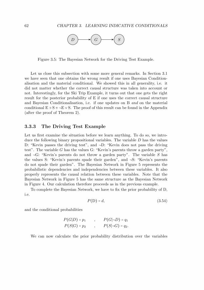
62 CHAPTER 3. LEARNING INDICATIVE CONDITIONALS
D G S
Figure 3.5: The Bayesian Network for the Driving Test Example.
Let us close this subsection with some more general remarks. In Section 3.1we have seen that one obtains the wrong result if one uses Bayesian Condition-alisation and the material conditional. We showed this in all generality, i.e. itdid not matter whether the correct causal structure was taken into account ornot. Interestingly, for the Ski Trip Example, it turns out that one gets the rightresult for the posterior probability of E if one uses the correct causal structureand Bayesian Conditionalisation, i.e. if one updates on B and on the materialconditional E ⊃ S ≡ ¬E ∨ S. The proof of this result can be found in the Appendix(after the proof of Theorem 2).
3.3.3 The Driving Test Example
Let us first examine the situation before we learn anything. To do so, we intro-duce the following binary propositional variables. The variable D has the valuesD: “Kevin passes the driving test”, and ¬D: “Kevin does not pass the drivingtest”. The variable G has the values G: “Kevin’s parents throw a garden party”,and ¬G: “Kevin’s parents do not throw a garden party”. The variable S hasthe values S: “Kevin’s parents spade their garden”, and ¬S: “Kevin’s parentsdo not spade their garden”. The Bayesian Network in Figure 5 represents theprobabilistic dependencies and independencies between these variables. It alsoproperly represents the causal relation between these variables. Note that theBayesian Network in Figure 5 has the same structure as the Bayesian Networkin Figure 4. Our calculation therefore proceeds as in the previous example.
To complete the Bayesian Network, we have to fix the prior probability of D,i.e.
P (D) = d, (3.54)
and the conditional probabilities
P (G∣D) = p1 , P (G∣¬D) = q1
P (S∣G) = p2 , P (S∣¬G) = q2.
We can now calculate the prior probability distribution over the variables
3.3. MEETING THE CHALLENGES 63
D,G and S:
P (D,G,S) = dp1 p2 , P (D,G,¬S) = dp1 p2
P (D,¬G,S) = dp1q2 , P (D,¬G,¬S) = dp1 q2
P (¬D,G,S) = d q1 p2 , P (¬D,G,¬S) = d q1 p2
P (¬D,¬G,S) = d q1 q2 , P (¬D,¬G,¬S) = d q1 q2 (3.55)
Next we learn two items of information, as a result of which our probabilitydistribution changes from P to P ′. First, we learn that S obtains. Assumingthat the causal structure depicted in Figure 5 does not change, this means thatwe learn that
P ′(S) = d′ (p′1 p′2 + p
′1q
′2) + d
′ (q′1 p′2 + q
′1q
′2) = 1 , (3.56)
where we have replaced all variables by the corresponding primed variables. Sec-ond, we learn the conditional “if Kevin passed the driving test, his parents willthrow a garden party”, which implies that
P ′(G∣D) = p′1 = 1. (3.57)
Inserting eq. (3.57) into eq. (3.56), we obtain:
d′ p′2 + d′ (q′1 p
′2 + q
′1 q
′2) = 1 (3.58)
This equation only holds for d′ ∈ (0,1), if
p′2 = 1 (3.59)
and ifq′1 p
′2 + q
′1 q
′2 ≡ q
′1 + q
′1 q
′2 = 1.
It has the solutions (i) q′1 = 1 and (ii) q′2 = 1. As solution (i) does not makesense intuitively, given the story (unless Kevin’s parents would have planned thegarden party independently), we conclude that
q′2 = 1. (3.60)
Inserting conditions (3.57), (3.59) and (3.60) into the analogues of eqs. (3.55),we can calculate the posterior probability distribution:
P ′(D,G,S) = d′ , P ′(D,G,¬S) = 0
P ′(D,¬G,S) = 0 , P ′(D,¬G,¬S) = 0
P ′(¬D,G,S) = d′ q′1 , P ′(¬D,G,¬S) = 0 (3.61)
P ′(¬D,¬G,S) = d′ q′1 , P (¬D,¬G,¬S) = 0
We can now show the following theorem (proof in the Appendix).
64 CHAPTER 3. LEARNING INDICATIVE CONDITIONALS
Theorem 3.3.3 Consider the Bayesian Network in Figure 5 with the prior prob-ability distribution from eq. (3.55). Let
k0 ∶=p1 p2
q1 p2 + q1 q2.
We furthermore assume that (i) the posterior probability distribution P ′ is definedover the same Bayesian Network, (ii) the learned information is modelled asconstraints (eqs. (3.56) and (3.57)) on P ′, and (iii) P ′ minimises the Kullback-Leibler divergence to P . Then P ′(D) < P (D), iff k0 < 1.
Note that it is clear from the story that q2 ≫ p2. Hence,
k0 <p1p2
q1p2 + q1p2=p1p2
p2= p1 < 1. (3.62)
We conclude that the posterior probability that Kevin passed the driving test issmaller than the prior probability. The proposed method yields the intuitivelycorrect result in this case.
3.3.4 The Judy Benjamin Problem
In our discussion of this problem in Section 2 we introduced two propositionalvariables, R and S. Before receiving the radio message, Judy considers the twovariables to be probabilistically independent. After receiving the radio message,they became probabilistically dependent. This probabilistic dependence (as wellas the probabilistic independence before receiving the message) can be repre-sented in the Bayesian Network in Figure 2. However, as should be clear bynow, this Bayesian Network does not reflect the causal relation between the twovariables: R does not cause S, and S does not cause R. Hence, there must beanother explanation for the probabilistic correlation – a common cause of R andS.
So let us introduce a new binary propositional variables X. Its values couldbe, for example, that there is wind from a certain direction (X), and that there isno wind from a certain direction (¬X). Note, however, that nothing hinges on thespecific values of X. All we need is that Judy believes that a common cause, andnot a direct causal relation, explains the learned probabilistic correlation betweenR and S. The Bayesian Network in Figure 6 represents this situation.
This move suggests the following strategy. The situation after receiving theradio message is represented by the Bayesian Network in Figure 6. The situa-tion before receiving the message can be represented by the Bayesian Networkin Figure 2 (with R and S being independent). However, for technical reasons9
9Calculating the Kullback-Leibler divergence between two probability distributions presup-poses that both distributions have the same number of atoms.
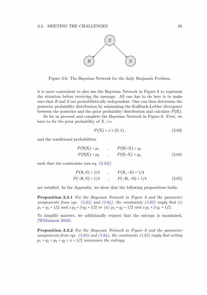
3.3. MEETING THE CHALLENGES 65
X
SR
Figure 3.6: The Bayesian Network for the Judy Benjamin Problem.
it is more convenient to also use the Bayesian Network in Figure 6 to representthe situation before receiving the message. All one has to do here is to makesure that R and S are probabilistically independent. One can then determine theposterior probability distribution by minimising the Kullback-Leibler divergencebetween the posterior and the prior probability distribution and calculate P (R).
So let us proceed and complete the Bayesian Network in Figure 6. First, wehave to fix the prior probability of X, i.e.
P (X) = x ∈ (0,1) , (3.63)
and the conditional probabilities
P (R∣X) = p1 , P (R∣¬X) = q1
P (S∣X) = p2 , P (S∣¬X) = q2 . (3.64)
such that the constraints (see eq. (3.24))
P (R,S) = 1/4 , P (R,¬S) = 1/4
P (¬R,S) = 1/4 , P (¬R,¬S) = 1/4 (3.65)
are satisfied. In the Appendix, we show that the following propositions holds.
Proposition 3.3.1 For the Bayesian Network in Figure 6 and the parameterassignments from eqs. (3.63) and (3.64), the constraints (3.65) imply that (i)p1 = q1 = 1/2 and xp2 + xq2 = 1/2 or (ii) p2 = q2 = 1/2 and xp1 + xq1 = 1/2.
To simplify matters, we additionally request that the entropy is maximised,(Williamson 2010).
Proposition 3.3.2 For the Bayesian Network in Figure 6 and the parameterassignments from eqs. (3.63) and (3.64), the constraints (3.65) imply that settingp1 = q1 = p2 = q2 = x = 1/2 maximises the entropy.
66 CHAPTER 3. LEARNING INDICATIVE CONDITIONALS
Next Judy learns that “if you are in Red Territory, then the odds are 3 ∶ 1that you are in Second Company area.” This is a constraint on the posteriorprobability distribution P ′, which implies that
P ′(S∣R) = k , (3.66)
with k ∈ IJB . In our specific case, we have k = 3/4, but (as above) we want tokeep things slightly more general by introducing the parameter k. We also noticethat the prior probability of X and the likelihoods may change and set
P ′(X) = x′ (3.67)
and
P ′(R∣X) =∶ p′1 , P ′(R∣¬X) =∶ q′1P ′(S∣X) =∶ p′2 , P ′(S∣¬X) =∶ q′2 . (3.68)
Note that x′, p′1, q′1, p
′2 and q′2 are not independent: They have to satisfy
the constraint (3.66).We can now show the following theorem (proof in the Ap-pendix).
Theorem 3.3.4 Consider the Bayesian Network in Figure 6 with the prior prob-ability distribution P satisfying Proposition 2. We furthermore assume that (i)P ′ is defined over the same Bayesian Network as P , (ii) the learned informa-tion is modelled as a constraint (eqs. (3.66)) on P ′, and (iii) P ′ minimises theKullback-Leibler divergence to P . Then P ′(R) = P (R).
3.4 Disabling Conditions
The analyses of the examples in the previous section presupposed that all relevantvariables can be read off from the story. In particular, we have assumed that thereare no interfering causes or disabling conditions that are not mentioned in thestory. Our analysis of the Ski Trip Example, for instance, assumed that thereis nothing that prevents the father from inviting Sue for a ski trip once he hasmade the promise. This may not be the case, and we may have beliefs about thepresence of a disabling condition. For example, we may consider the possibilitythat Sue’s father changes his mind or that he looses all his money so that hecannot cover the costs of Sue’s ski trip anymore. It is also possible that he hasan accident or even dies before he can fulfil his promise. In this section, we showhow such disabling conditions can be modelled in a straightforward way. To doso, we focus on the Ski Trip Example.
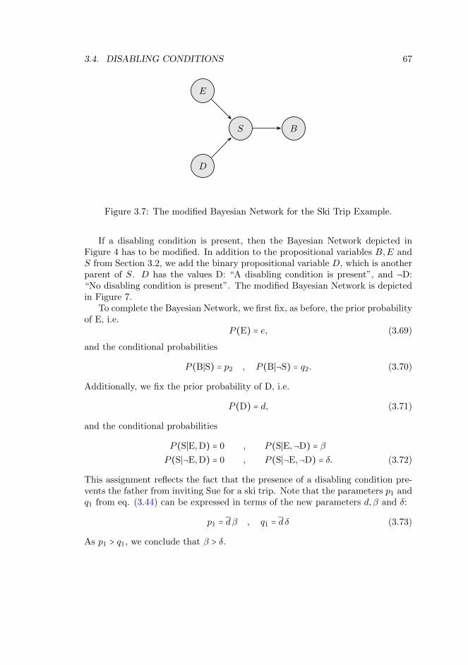
3.4. DISABLING CONDITIONS 67
E
S
D
B
Figure 3.7: The modified Bayesian Network for the Ski Trip Example.
If a disabling condition is present, then the Bayesian Network depicted inFigure 4 has to be modified. In addition to the propositional variables B,E andS from Section 3.2, we add the binary propositional variable D, which is anotherparent of S. D has the values D: “A disabling condition is present”, and ¬D:“No disabling condition is present”. The modified Bayesian Network is depictedin Figure 7.
To complete the Bayesian Network, we first fix, as before, the prior probabilityof E, i.e.
P (E) = e, (3.69)
and the conditional probabilities
P (B∣S) = p2 , P (B∣¬S) = q2. (3.70)
Additionally, we fix the prior probability of D, i.e.
P (D) = d, (3.71)
and the conditional probabilities
P (S∣E,D) = 0 , P (S∣E,¬D) = β
P (S∣¬E,D) = 0 , P (S∣¬E,¬D) = δ. (3.72)
This assignment reflects the fact that the presence of a disabling condition pre-vents the father from inviting Sue for a ski trip. Note that the parameters p1 andq1 from eq. (3.44) can be expressed in terms of the new parameters d, β and δ:
p1 = dβ , q1 = d δ (3.73)
As p1 > q1, we conclude that β > δ.
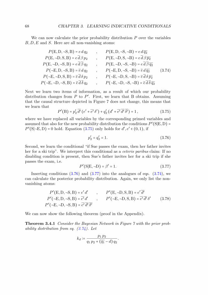
68 CHAPTER 3. LEARNING INDICATIVE CONDITIONALS
We can now calculate the prior probability distribution P over the variablesB,D,E and S. Here are all non-vanishing atoms:
P (E,D,¬S,B) = e d q2 , P (E,D,¬S,¬B) = e d q2
P (E,¬D,S,B) = e dβ p2 , P (E,¬D,S,¬B) = e dβ p2
P (E,¬D,¬S,B) = e dβ q2 , P (E,¬D,¬S,¬B) = e dβ q2
P (¬E,D,¬S,B) = e d q2 , P (¬E,D,¬S,¬B) = e d q2 (3.74)
P (¬E,¬D,S,B) = e d δ p2 , P (¬E,¬D,S,¬B) = e d δ p2
P (¬E,¬D,¬S,B) = e d δ q2 , P (¬E,¬D,¬S,¬B) = e d δ q2
Next we learn two items of information, as a result of which our probabilitydistribution changes from P to P ′. First, we learn that B obtains. Assumingthat the causal structure depicted in Figure 7 does not change, this means thatwe learn that
P ′(B) = p′2 d′ (e′ + e′ δ′) + q′2 (d′ + e′ d′ δ′) = 1 , (3.75)
where we have replaced all variables by the corresponding primed variables andassumed that also for the new probability distribution the conditions P ′(S∣E,D) =P ′(S∣¬E,D) = 0 hold. Equation (3.75) only holds for d′, e′ ∈ (0,1), if
p′2 = q′2 = 1. (3.76)
Second, we learn the conditional “if Sue passes the exam, then her father invitesher for a ski trip”. We interpret this conditional as a ceteris paribus claim: If nodisabling condition is present, then Sue’s father invites her for a ski trip if shepasses the exam, i.e.
P ′(S∣E,¬D) = β′ = 1. (3.77)
Inserting conditions (3.76) and (3.77) into the analogues of eqs. (3.74), wecan calculate the posterior probability distribution. Again, we only list the non-vanishing atoms:
P ′(E,D,¬S,B) = e′ d′ , P ′(E,¬D,S,B) = e′ d′
P ′(¬E,D,¬S,B) = e′ d′ , P ′(¬E,¬D,S,B) = e′ d′ δ′ (3.78)
P ′(¬E,¬D,¬S,B) = e′ d′ δ′
We can now show the following theorem (proof in the Appendix).
Theorem 3.4.1 Consider the Bayesian Network in Figure 7 with the prior prob-ability distribution from eq. (3.74). Let
kd ∶=p1 p2
q1 p2 + (q1 − d) q2.
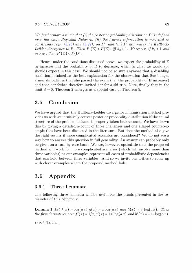
3.5. CONCLUSION 69
We furthermore assume that (i) the posterior probability distribution P ′ is definedover the same Bayesian Network, (ii) the learned information is modelled asconstraints (eqs. (3.76) and (3.77)) on P ′, and (iii) P ′ minimises the Kullback-Leibler divergence to P . Then P ′(E) > P (E), iff kd > 1. Moreover, if kd > 1 andp2 > q2, then P ′(D) < P (D).
Hence, under the conditions discussed above, we expect the probability of Eto increase and the probability of D to decrease, which is what we would (orshould) expect in this case. We should not be so sure anymore that a disablingcondition obtained as the best explanation for the observation that Sue boughta new ski outfit is that she passed the exam (i.e. the probability of E increases)and that her father therefore invited her for a ski trip. Note, finally that in thelimit d→ 0, Theorem 2 emerges as a special case of Theorem 5.
3.5 Conclusion
We have argued that the Kullback-Leibler divergence minimisation method pro-vides us with an intuitively correct posterior probability distribution if the causalstructure of the problem at hand is properly taken into account. We have shownthis by giving a detailed account of three challenges and one alleged counterex-ample that have been discussed in the literature. But does the method also givethe right results if more complicated scenarios are considered? We do not see away how to answer this question in full generality. An answer can probably onlybe given on a case-by-case basis. We are, however, optimistic that the proposedmethod will work for more complicated scenarios (which will involve more thanthree variables) as our examples represent all cases of probabilistic dependenciesthat can hold between three variables. And so we invite our critics to come upwith clever examples where the proposed method fails.
3.6 Appendix
3.6.1 Three Lemmata
The following three lemmata will be useful for the proofs presented in the re-mainder of this Appendix.
Lemma 1 Let f(x) ∶= log(ax), g(x) ∶= x log(ax) and h(x) ∶= x log(ax). Thenthe first derivatives are: f ′(x) = 1/x, g′(x) = 1+ log(ax) and h′(x) = −1−log(ax).
Proof: Trivial.
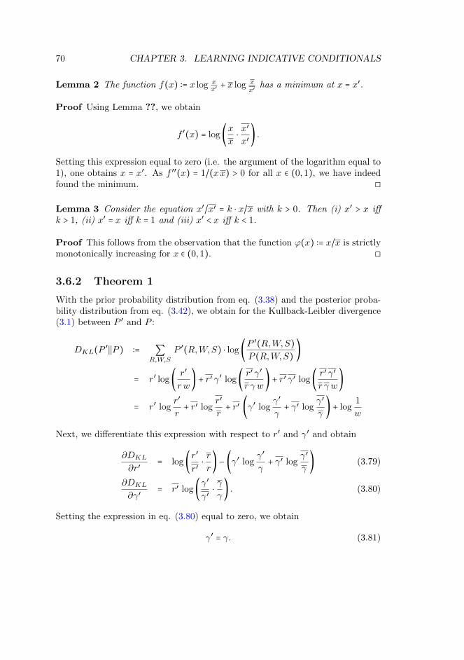
70 CHAPTER 3. LEARNING INDICATIVE CONDITIONALS
Lemma 2 The function f(x) ∶= x log xx′ + x log x
x′has a minimum at x = x′.
Proof Using Lemma ??, we obtain
f ′(x) = log(x
x⋅x′
x′) .
Setting this expression equal to zero (i.e. the argument of the logarithm equal to1), one obtains x = x′. As f ′′(x) = 1/(xx) > 0 for all x ∈ (0,1), we have indeedfound the minimum. ◻
Lemma 3 Consider the equation x′/x′ = k ⋅ x/x with k > 0. Then (i) x′ > x iffk > 1, (ii) x′ = x iff k = 1 and (iii) x′ < x iff k < 1.
Proof This follows from the observation that the function ϕ(x) ∶= x/x is strictlymonotonically increasing for x ∈ (0,1). ◻
3.6.2 Theorem 1
With the prior probability distribution from eq. (3.38) and the posterior proba-bility distribution from eq. (3.42), we obtain for the Kullback-Leibler divergence(3.1) between P ′ and P :
DKL(P′∣∣P ) ∶= ∑
R,W,S
P ′(R,W,S) ⋅ log(P ′(R,W,S)
P (R,W,S))
= r′ log(r′
r w) + r′ γ′ log(
r′ γ′
r γ w) + r′ γ′ log(
r′ γ′
r γ w)
= r′ logr′
r+ r′ log
r′
r+ r′ (γ′ log
γ′
γ+ γ′ log
γ′
γ) + log
1
w
Next, we differentiate this expression with respect to r′ and γ′ and obtain
∂DKL
∂r′= log(
r′
r′⋅r
r) − (γ′ log
γ′
γ+ γ′ log
γ′
γ) (3.79)
∂DKL
∂γ′= r′ log(
γ′
γ′⋅γ
γ) . (3.80)
Setting the expression in eq. (3.80) equal to zero, we obtain
γ′ = γ. (3.81)
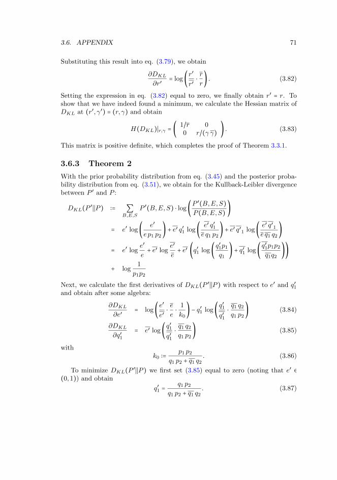
3.6. APPENDIX 71
Substituting this result into eq. (3.79), we obtain
∂DKL
∂r′= log(
r′
r′⋅r
r) . (3.82)
Setting the expression in eq. (3.82) equal to zero, we finally obtain r′ = r. Toshow that we have indeed found a minimum, we calculate the Hessian matrix ofDKL at (r′, γ′) = (r, γ) and obtain
H(DKL)∣r,γ = (1/r 00 r/(γ γ)
) . (3.83)
This matrix is positive definite, which completes the proof of Theorem 3.3.1.
3.6.3 Theorem 2
With the prior probability distribution from eq. (3.45) and the posterior proba-bility distribution from eq. (3.51), we obtain for the Kullback-Leibler divergencebetween P ′ and P :
DKL(P′∣∣P ) ∶= ∑
B,E,S
P ′(B,E,S) ⋅ log(P ′(B,E,S)
P (B,E,S))
= e′ log(e′
e p1 p2) + e′ q′1 log(
e′ q′1e q1 p2
) + e′ q′1 log(e′ q′1e q1 q2
)
= e′ loge′
e+ e′ log
e′
e+ e′ (q′1 log(
q′1p1
q1) + q′1 log(
q′1p1p2
q1q2))
+ log1
p1p2
Next, we calculate the first derivatives of DKL(P′∣∣P ) with respect to e′ and q′1
and obtain after some algebra:
∂DKL
∂e′= log(
e′
e′⋅e
e⋅
1
k0) − q′1 log(
q′1q′1
⋅q1 q2
q1 p2) (3.84)
∂DKL
∂q′1= e′ log(
q′1q′1
⋅q1 q2
q1 p2) (3.85)
withk0 ∶=
p1 p2
q1 p2 + q1 q2. (3.86)
To minimize DKL(P′∣∣P ) we first set (3.85) equal to zero (noting that e′ ∈
(0,1)) and obtain
q′1 =q1 p2
q1 p2 + q1 q2. (3.87)
72 CHAPTER 3. LEARNING INDICATIVE CONDITIONALS
With this, we simplify the expression in eq. (3.84) and obtain
∂DKL
∂e′= log(
e′
e′⋅e
e⋅
1
k0) . (3.88)
Setting now also the expression in eq. (3.88) to zero, we obtain
e′
e′= k0 ⋅
e
e. (3.89)
Using Lemma 3, we conclude that e′ > e iff k0 > 1. This completes the proof ofTheorem 3.3.2. (We skip the proof that the corresponding Hessian is positivedefinite if eqs. (3.87) and (3.89) hold.)
Let us now calculate the posterior probability of E after learning B and thematerial conditional E ⊃ S ≡ ¬E ∨ S. We obtain
P ∗(E) = P (E∣B ∧ (¬E ∨ S)) =P (E ∧B ∧ (¬E ∨ S))
P (B ∧ (¬E ∨ S))
=P (B ∧E ∧ S)
P ((B ∧ ¬E) ∨ (B ∧ S))=
P (B,E,S)
P (B,¬E) + P (B,S) − P (B,¬E,S)
=P (B,E,S)
P (B,¬E) + P (B,E,S). (3.90)
With the Bayesian Network depicted in Figure 4 and the prior probability dis-tribution from eq. (3.45), we then obtain
P ∗(E) =e p1 p2
e p1 p2 + e (q1 p2 + q1 q2)=
e k0
e k0 + e≡ e′ = P ′(E). (3.91)
From this equation it is easy to see that P ∗(E) > P (E) iff k0 > 1. Hence, bothprocedures yield exactly the same result in this case.
3.6.4 Theorem 3
The proof of Theorem 3.3.3 is analogous to the proof of Theorem 3.3.2. With theprior probability distribution from eq. (3.55) and the posterior probability dis-tribution from eq. (3.61), we obtain for the Kullback-Leibler divergence between
3.6. APPENDIX 73
P ′ and P :
DKL(P′∣∣P ) ∶= ∑
D,G,S
P ′(D,G,S) ⋅ log(P ′(D,G,S)
P (D,G,S))
= d′ log(d′
dp1 p2) + d′ q′1 log(
e′ q′1d q1 p2
) + d′ q′1 log(d′ q′1d q1 q2
)
= d′ logd′
d+ d′ log
d′
d+ d′ (q′1 log(
q′1p1
q1) + q′1 log(
q′1p1p2
q1q2))
+ log1
p1p2
Next, we calculate the first derivatives of DKL(P′∣∣P ) with respect to d′ and q′1
and obtain after some algebra
∂DKL
∂d′= log(
d′
d′⋅d
d⋅
1
k0) − q′1 log(
q′1q′1
⋅q1 q2
q1 p2) (3.92)
∂DKL
∂q′1= d′ log(
q′1q′1
⋅q1 q2
q1 p2) , (3.93)
withk0 ∶=
p1 p2
q1 p2 + q1 q2. (3.94)
To minimize DKL(P′∣∣P ) we first set (3.93) equal to zero (noting that d′ ∈
(0,1)) and obtain
q′1 =q1 p2
q1 p2 + q1 q2. (3.95)
With this, we simplify the expression in eq. (3.92) and obtain
∂DKL
∂d′= log(
d′
d′⋅d
d⋅
1
k0) . (3.96)
Setting now also the expression in eq. (3.96) to zero, we obtain
d′
d′= k0 ⋅
d
d. (3.97)
Using Lemma 3, we conclude that d′ < d iff k0 < 1. This completes the proofof Theorem 3.3.3. (We skip the proof that the corresponding Hessian is positivedefinite if eqs. (3.95) and (3.97) hold.)
Again, using the material conditional yields exactly the same result (and thecalculation is analogous to the one at the end of the proof of Theorem 3.3.2).
74 CHAPTER 3. LEARNING INDICATIVE CONDITIONALS
3.6.5 Proposition 1
From the Bayesian Network in Figure 6 and the constraints (3.65), we obtain:
xp1p2 + xq1q2 = 1/4 (3.98)
xp1p2 + xq1q2 = 1/4 (3.99)
xp1p2 + xq1q2 = 1/4 (3.100)
xp1p2 + xq1q2 = 1/4 (3.101)
We now add eqs. (3.98) and (3.99) as well as eqs. (3.100) and (3.101) andobtain:
xp1 + xq1 = 1/2 (3.102)
xp1 + xq1 = 1/2 (3.103)
Note that eq. (3.103) follows from eq. (3.102). Similarly, by adding eqs. (3.98)and (3.100) as well as eqs. (3.99) and (3.101), we obtain:
xp2 + xq2 = 1/2 (3.104)
We now solve eq. (3.102) for q1 and eq. (3.104) for q2 and insert the resultingexpressions in eqs. (3.98) to (3.101). In each case, we obtain:
(p1 − 1/2)(p2 − 1/2) = 0 (3.105)
This equation has two solutions, viz. (i) p1 = 1/2 and (ii) p2 = 1/2. Using eqs.(3.102) and (3.104) completes the proof of Proposition 3.3.1.
3.6.6 Proposition 2
We begin with solution (i) from Proposition 3.3.1 and construct the prior prob-ability distribution.
P (X,R,S) = 1/2xp2 , P (X,R,¬S) = 1/2xp2
P (X,¬R,S) = 1/2xp2 , P (X,¬R,¬S) = 1/2xp2
P (¬X,R,S) = 1/2xq2 , P (¬X,R,¬S) = 1/2xq2 (3.106)
P (¬X,¬R,S) = 1/2xq2 , P (¬X,¬R,¬S) = 1/2xq2.
With this, we calculate the entropy
S = − ∑X,R,S
P (X,R,S) ⋅ logP (X,R,S) (3.107)
3.6. APPENDIX 75
and obtain
S = −(x logx + x logx) − x (p2 log p2 + p2 log p2) − x (q2 log q2 + q2 log q2) + log 2.(3.108)
We want to maximize S under the constraint
xp2 + xq2 = 1/2. (3.109)
To do so, we use the method of Lagrange multipliers and first calculate thederivates of
L = S − λ (xp2 + xq2 − 1/2) (3.110)
with respect to p2 and q2. We obtain
∂L
∂p2= −x(log
p2
p2+ λ) (3.111)
∂L
∂q2= −x(log
q2
q2+ λ) . (3.112)
Setting these expressions equal to zero and taking into account that x ∈ (0,1),we obtain
p2 = q2 =1
1 + eλ. (3.113)
Inserting this into eq. (3.109), we obtain
p2 = q2 = 1/2, (3.114)
and hence λ = 0. Inserting all this into eq. (3.110), we obtain
L = 2 log 2 − (x logx + x logx), (3.115)
which maximizes at x = 1/2 (cf Lemma 2).The calculation for solution (ii) proceeds analogously for reasons of symmetry.
This completes the proof of Proposition 3.3.2.
3.6.7 Theorem 4
Let us first calculate the prior probability distribution over the variables X,Rand S with the parameters given in Proposition 3.3.2:
P (X,R,S) = 1/8 , P (X,R,¬S) = 1/8
P (X,¬R,S) = 1/8 , P (X,¬R,¬S) = 1/8
P (¬X,R,S) = 1/8 , P (¬X,R,¬S) = 1/8 (3.116)
P (¬X,¬R,S) = 1/8 , P (¬X,¬R,¬S) = 1/8
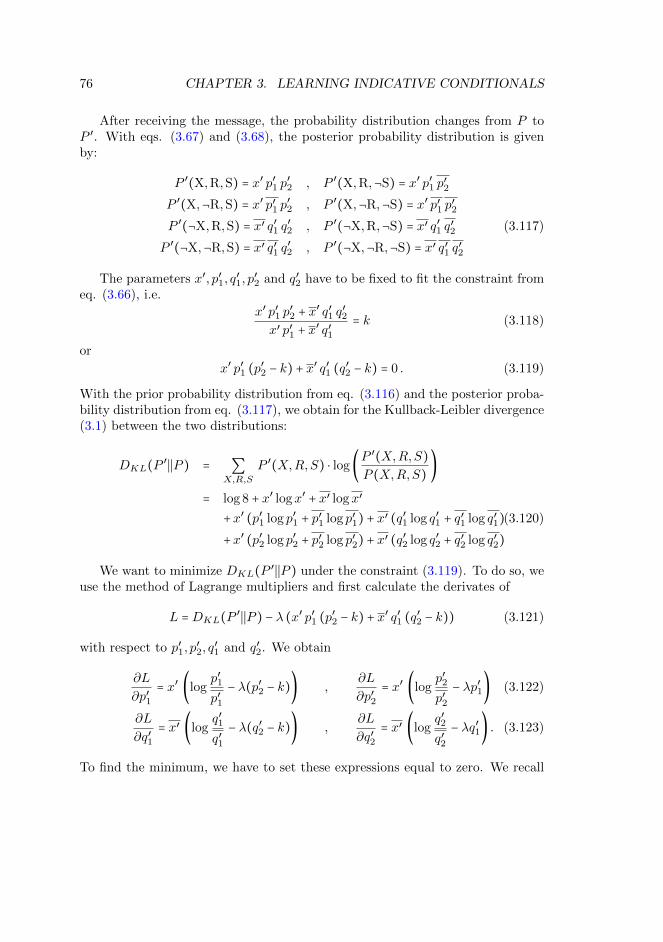
76 CHAPTER 3. LEARNING INDICATIVE CONDITIONALS
After receiving the message, the probability distribution changes from P toP ′. With eqs. (3.67) and (3.68), the posterior probability distribution is givenby:
P ′(X,R,S) = x′ p′1 p′2 , P ′(X,R,¬S) = x′ p′1 p
′2
P ′(X,¬R,S) = x′ p′1 p′2 , P ′(X,¬R,¬S) = x′ p′1 p
′2
P ′(¬X,R,S) = x′ q′1 q′2 , P ′(¬X,R,¬S) = x′ q′1 q
′2 (3.117)
P ′(¬X,¬R,S) = x′ q′1 q′2 , P ′(¬X,¬R,¬S) = x′ q′1 q
′2
The parameters x′, p′1, q′1, p
′2 and q′2 have to be fixed to fit the constraint from
eq. (3.66), i.e.
x′ p′1 p′2 + x
′ q′1 q′2
x′ p′1 + x′ q′1
= k (3.118)
or
x′ p′1 (p′2 − k) + x′ q′1 (q′2 − k) = 0 . (3.119)
With the prior probability distribution from eq. (3.116) and the posterior proba-bility distribution from eq. (3.117), we obtain for the Kullback-Leibler divergence(3.1) between the two distributions:
DKL(P′∣∣P ) = ∑
X,R,S
P ′(X,R,S) ⋅ log(P ′(X,R,S)
P (X,R,S))
= log 8 + x′ logx′ + x′ logx′
+x′ (p′1 log p′1 + p′1 log p′1) + x
′ (q′1 log q′1 + q′1 log q′1)(3.120)
+x′ (p′2 log p′2 + p′2 log p′2) + x
′ (q′2 log q′2 + q′2 log q′2)
We want to minimize DKL(P′∣∣P ) under the constraint (3.119). To do so, we
use the method of Lagrange multipliers and first calculate the derivates of
L =DKL(P′∣∣P ) − λ (x′ p′1 (p′2 − k) + x
′ q′1 (q′2 − k)) (3.121)
with respect to p′1, p′2, q
′1 and q′2. We obtain
∂L
∂p′1= x′ (log
p′1p′1
− λ(p′2 − k)) ,∂L
∂p′2= x′ (log
p′2p′2
− λp′1) (3.122)
∂L
∂q′1= x′ (log
q′1q′1
− λ(q′2 − k)) ,∂L
∂q′2= x′ (log
q′2q′2
− λq′1) . (3.123)
To find the minimum, we have to set these expressions equal to zero. We recall
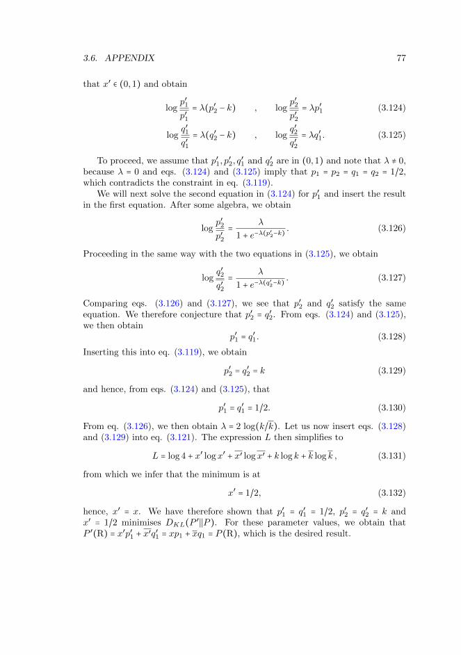
3.6. APPENDIX 77
that x′ ∈ (0,1) and obtain
logp′1p′1
= λ(p′2 − k) , logp′2p′2
= λp′1 (3.124)
logq′1q′1
= λ(q′2 − k) , logq′2q′2
= λq′1. (3.125)
To proceed, we assume that p′1, p′2, q
′1 and q′2 are in (0,1) and note that λ ≠ 0,
because λ = 0 and eqs. (3.124) and (3.125) imply that p1 = p2 = q1 = q2 = 1/2,which contradicts the constraint in eq. (3.119).
We will next solve the second equation in (3.124) for p′1 and insert the resultin the first equation. After some algebra, we obtain
logp′2p′2
=λ
1 + e−λ(p′2−k)
. (3.126)
Proceeding in the same way with the two equations in (3.125), we obtain
logq′2q′2
=λ
1 + e−λ(q′2−k)
. (3.127)
Comparing eqs. (3.126) and (3.127), we see that p′2 and q′2 satisfy the sameequation. We therefore conjecture that p′2 = q′2. From eqs. (3.124) and (3.125),we then obtain
p′1 = q′1. (3.128)
Inserting this into eq. (3.119), we obtain
p′2 = q′2 = k (3.129)
and hence, from eqs. (3.124) and (3.125), that
p′1 = q′1 = 1/2. (3.130)
From eq. (3.126), we then obtain λ = 2 log(k/k). Let us now insert eqs. (3.128)and (3.129) into eq. (3.121). The expression L then simplifies to
L = log 4 + x′ logx′ + x′ logx′ + k log k + k log k , (3.131)
from which we infer that the minimum is at
x′ = 1/2, (3.132)
hence, x′ = x. We have therefore shown that p′1 = q′1 = 1/2, p′2 = q′2 = k andx′ = 1/2 minimises DKL(P
′∣∣P ). For these parameter values, we obtain thatP ′(R) = x′p′1 + x
′q′1 = xp1 + xq1 = P (R), which is the desired result.
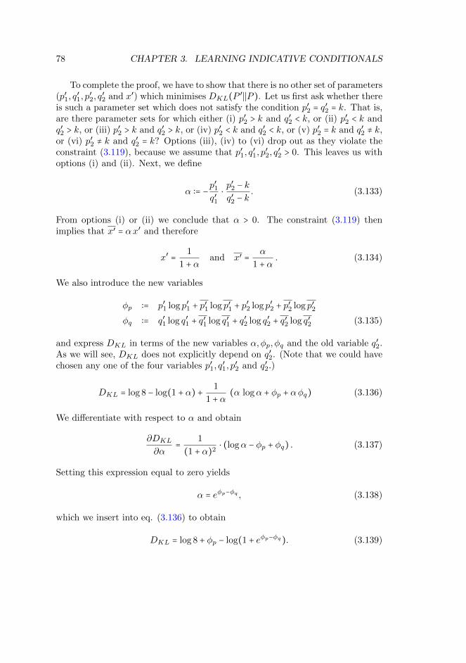
78 CHAPTER 3. LEARNING INDICATIVE CONDITIONALS
To complete the proof, we have to show that there is no other set of parameters(p′1, q
′1, p
′2, q
′2 and x′) which minimises DKL(P
′∣∣P ). Let us first ask whether thereis such a parameter set which does not satisfy the condition p′2 = q
′2 = k. That is,
are there parameter sets for which either (i) p′2 > k and q′2 < k, or (ii) p′2 < k andq′2 > k, or (iii) p′2 > k and q′2 > k, or (iv) p′2 < k and q′2 < k, or (v) p′2 = k and q′2 ≠ k,or (vi) p′2 ≠ k and q′2 = k? Options (iii), (iv) to (vi) drop out as they violate theconstraint (3.119), because we assume that p′1, q
′1, p
′2, q
′2 > 0. This leaves us with
options (i) and (ii). Next, we define
α ∶= −p′1q′1
⋅p′2 − k
q′2 − k. (3.133)
From options (i) or (ii) we conclude that α > 0. The constraint (3.119) thenimplies that x′ = αx′ and therefore
x′ =1
1 + αand x′ =
α
1 + α. (3.134)
We also introduce the new variables
φp ∶= p′1 log p′1 + p′1 log p′1 + p
′2 log p′2 + p
′2 log p′2
φq ∶= q′1 log q′1 + q′1 log q′1 + q
′2 log q′2 + q
′2 log q′2 (3.135)
and express DKL in terms of the new variables α,φp, φq and the old variable q′2.As we will see, DKL does not explicitly depend on q′2. (Note that we could havechosen any one of the four variables p′1, q
′1, p
′2 and q′2.)
DKL = log 8 − log(1 + α) +1
1 + α(α logα + φp + αφq) (3.136)
We differentiate with respect to α and obtain
∂DKL
∂α=
1
(1 + α)2⋅ (logα − φp + φq) . (3.137)
Setting this expression equal to zero yields
α = eφp−φq , (3.138)
which we insert into eq. (3.136) to obtain
DKL = log 8 + φp − log(1 + eφp−φq). (3.139)
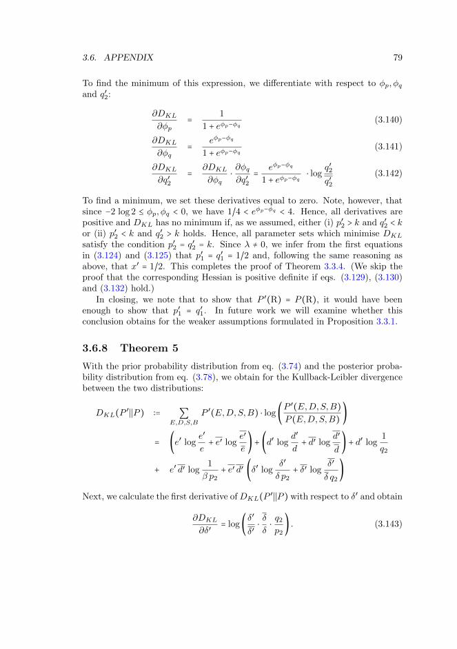
3.6. APPENDIX 79
To find the minimum of this expression, we differentiate with respect to φp, φqand q′2:
∂DKL
∂φp=
1
1 + eφp−φq(3.140)
∂DKL
∂φq=
eφp−φq
1 + eφp−φq(3.141)
∂DKL
∂q′2=
∂DKL
∂φq⋅∂φq
∂q′2=
eφp−φq
1 + eφp−φq⋅ log
q′2q′2
(3.142)
To find a minimum, we set these derivatives equal to zero. Note, however, thatsince −2 log 2 ≤ φp, φq < 0, we have 1/4 < eφp−φq < 4. Hence, all derivatives arepositive and DKL has no minimum if, as we assumed, either (i) p′2 > k and q′2 < kor (ii) p′2 < k and q′2 > k holds. Hence, all parameter sets which minimise DKL
satisfy the condition p′2 = q′2 = k. Since λ ≠ 0, we infer from the first equationsin (3.124) and (3.125) that p′1 = q′1 = 1/2 and, following the same reasoning asabove, that x′ = 1/2. This completes the proof of Theorem 3.3.4. (We skip theproof that the corresponding Hessian is positive definite if eqs. (3.129), (3.130)and (3.132) hold.)
In closing, we note that to show that P ′(R) = P (R), it would have beenenough to show that p′1 = q′1. In future work we will examine whether thisconclusion obtains for the weaker assumptions formulated in Proposition 3.3.1.
3.6.8 Theorem 5
With the prior probability distribution from eq. (3.74) and the posterior proba-bility distribution from eq. (3.78), we obtain for the Kullback-Leibler divergencebetween the two distributions:
DKL(P′∣∣P ) ∶= ∑
E,D,S,B
P ′(E,D,S,B) ⋅ log(P ′(E,D,S,B)
P (E,D,S,B))
= (e′ loge′
e+ e′ log
e′
e) + (d′ log
d′
d+ d′ log
d′
d) + d′ log
1
q2
+ e′ d′ log1
β p2+ e′ d′ (δ′ log
δ′
δ p2+ δ′ log
δ′
δ q2
)
Next, we calculate the first derivative of DKL(P′∣∣P ) with respect to δ′ and obtain
∂DKL
∂δ′= log(
δ′
δ′⋅δ
δ⋅q2
p2) . (3.143)
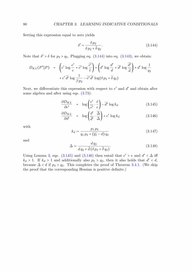
80 CHAPTER 3. LEARNING INDICATIVE CONDITIONALS
Setting this expression equal to zero yields
δ′ =δ p2
δ p2 + δ q2
. (3.144)
Note that δ′ > δ for p2 > q2. Plugging eq. (3.144) into eq. (3.143), we obtain:
DKL(P′∣∣P ) = (e′ log
e′
e+ e′ log
e′
e) + (d′ log
d′
d+ d′ log
d′
d) + d′ log
1
q2
+ e′ d′ log1
β p2− e′ d′ log(δ p2 + δ q2)
Next, we differentiate this expression with respect to e′ and d′ and obtain aftersome algebra and after using eqs. (3.73):
∂DKL
∂e′= log(
e′
e′⋅e
e) − d′ log kd (3.145)
∂DKL
∂d′= log(
d′
d′⋅∆
∆) + e′ log kd (3.146)
withkd ∶=
p1 p2
q1 p2 + (q1 − d) q2(3.147)
and
∆ ∶=d q2
d q2 + d (δ p2 + δ q2). (3.148)
Using Lemma 3, eqs. (3.145) and (3.146) then entail that e′ > e and d′ < ∆ iffkd > 1. If kd > 1 and additionally also p2 > q2, then it also holds that d′ < d,because ∆ < d if p2 > q2. This completes the proof of Theorem 3.4.1. (We skipthe proof that the corresponding Hessian is positive definite.)
Chapter 4
Voting, Deliberation AndTruth
4.1 Introduction
Consider a group aiming to make a collective decision on a binary choice prob-lem. There are countless examples of such scenarios and different methods andprocedures have been proposed and practiced for this purpose in large and smallscales. The most suitable procedure will no doubt depend on the type of thegroup, the kind of problem that the group deals with and the purpose of the col-lective decision. Thus let’s consider a group of autonomous, independent decisionmakers who make non-strategic individual judgments and who wish to arrive ata collective decision that best approximates some objective truth and, withoutany attempt to give a precise definition or characterisation of democracy, let’sassume that the group wishes to make the decision democratically.
There are at least two ways for the group to come to a collective decision:they can each cast a vote and then use some voting rule to aggregate the votesinto a collective choice. The majority rule is one example (probably the mostwidely practiced example) of a democratic voting rule. Alternatively, the groupmembers can deliberate, they present their arguments and reasons to the others,and eventually arrive at a unanimous verdict – a consensus.
Many examples of collective decision making deal with the aggregation ofpreferences with no external or objective reference for evaluation. In such casesthe decision making procedure is hence preferred on the basis of some collectivelyagreed upon desiderata. There are, on the other hand, instances that the decisionmakers aim, or are expected to aim, at the best approximation of some fact or
81
82 CHAPTER 4. VOTING, DELIBERATION AND TRUTH
truth. Juries in court are relevant examples of this: They are expected to convictthe guilty, and only the guilty. Expert committees (e.g. on environmental issues)are other cases in point. In these cases, the chosen decision making procedureshould facilitate this goal.
Hence, there are (at least) two distinct conceptions of how collective deci-sion rules can be evaluated and justified: the proceduralist conception and theepistemic conception. According to proceduralist view, the merit of a decisionmaking procedure depends only on its procedural characteristics. The work ofKenneth Arrow and his followers is a famous case in point. According to this viewthe desirability of a collective decision stems from the procedural characteristicsof the method itself and from the desiderata satisfied by the procedure, withoutany concerns of tracking some independent truth. According to the epistemicconception, on the other hand, the procedural characteristics are not enough forlegitimising a decision making procedure. Here the main concern is to apply amethod that provides reliable and correct outcomes and a decision making pro-cedure is preferred on the basis of its ability to do just this. One widely debatedway to put this comparison in perspective in to ask: What should constitute ourmain criteria for collective decision making? – The fairness of the procedure orthe correctness of the resulting decision?
Deliberative accounts of democratic decision making (deliberative democracy)present an immediate advantage over voting from the proceduralist point of view.This advantage is summarised in the formation of a group consensus. It eliminatesthe necessity for a compromise that is inevitable in voting scenarios. Indeed theprospect of a collective consensus on which all the group members agree uponis an attractive ideal of the proceduralist account. In this sense the deliberativeaccount performs more favourably than voting from the proceduralist perspective.
On the other hand, voting has strong epistemic support. The literature on theepistemic characteristics of majority voting is extensive, much of which is built onthe Condorcet Jury Theorem. In its original form the Condorcet Jury Theoremasserts that for a group of independent voters with reliabilities above 50% whoare faced with a binary choice problem, the probability that the majority votecoincides with the correct choice increases strictly monotonously with the size ofthe group and approaches 1 asymptotically. This result has since been improvedin the work of social choice theorists who have generalised and modified it torelax the assumptions. For example, List & Goodin generalised the theorem tocases with more than two choice options (List & Goodin 2001). It has also beenshown that the conclusion of the theorem holds if one requests that the averagereliability of all (independent) group members is greater than 0.5, and in recentwork Dietrich and Spiekermann proved a modified version of the Condorcet JuryTheorem where they differentiate between individual dependencies and depen-dencies on a common cause, (Douven 2012). There is, however, as mentioned
4.1. INTRODUCTION 83
above, a procedural disadvantage to majority voting, namely that the process ofvoting does not affect the epistemic state of the voters. With this considerationthe majority voting will always result in a minority that should comply with thevote of the majority as the collective decision while maintaining their original be-liefs. As such it will inevitably result in a compromise or possibly in a persistingconflict.
Our goal in this study is to investigate the deliberative account from an epis-temic point of view. We ask: is it also epistemically advantageous to deliberate,or is this procedure only preferable from a proceduralist point of view? The ques-tion is whether or not the procedural advantages of the deliberation process canbe backed with epistemic support to compare with majority voting. The idea of adeliberation process is to give the group members the opportunity to revise theirbeliefs in the light of the information they receive from their fellow group mem-bers, and ideally, come to an agreement on what the collective decision should be.There is an extensive literature on the epistemic analysis of deliberation, devel-oped in the works of scholars such as Joshua Cohen, David Estlund, and CarlosNino.1 This literature is concerned with justifying the deliberative account byclaiming epistemic advantage for the decisions made through a deliberation byadhering to the qualitative properties of the process in general; properties suchas better availability of information, facilitation of the analysis of arguments andreasons resulting in a higher chance of identifying mistakes and errors, reducingthe chance of manipulation by controlling the flow of information, etc.2
An important aspect, however, that bears on the epistemic analysis of de-liberation, is the way that the deliberation process is carried out. There are ofcourse different ways in which the group members can update their belief basedthe opinions of others and there are also different attributes of decision makersthat can be regarded relevant to the deliberation process. To make an investiga-tion of the epistemic behaviour of the deliberation one thus needs to first decideon how to formulate the deliberation procedure in detail.
There are several attempts in the literature for developinga formal account of rational deliberation, including the Lehrer-Wagner model (Lehrer & Wagner 1981), the Hegselmann-Krause model(Hegselmann & Krause 2002), and more recently the Laputa model developedat Lund University. These models focus on different characteristics of the delib-erating group members and deal with different contexts of decision making, butonly the Laputa model, amongst these, is built on Bayesian foundations. Olssonand co-authors have developed a detailed Bayesian model for the epistemic
1See (Cohen 1989a; Cohen 1989b), (Estlund 1993; Estlund 1994; Estlund 1997),(Manin 1987), and (Nino 1996).
2See (Bohman & Rehg 1997), (Cohen 1989a), (Dryzek 1990), (Elster 1998), (Fearon 1998),(Marti 2006), and (Nino 1996).
84 CHAPTER 4. VOTING, DELIBERATION AND TRUTH
interaction between the group members in which they allow for consideration ofany particular network configuration governing the flow of information in thegroup. In particular group members might only receive messages from someother group members or have different chances of receiving information fromone group member as opposed to another. The model also allows for somepersonal characteristics of the group members outside the social network, viz.the chance that they would engage an enquiry concerning the matter from someoutside source (their activity) and the chance that such enquiry would providethem with the right answer (their aptitude). This model provides an excellentframework for studying epistemic interactions in cases where group membershave limitations (imposed by some network configuration) in accessing eachothers’ opinions. Of course the case where group members receive informationfrom all others is a special case of the model. Here we will not give an overviewof the intricacies of the Laputa model and its applications and refer the readerto the literature.3
In our own model, however, we focus on cases where the group membersreceive no information from any outside source and the communication betweenthe different group members is open to all. This is in particular the case forjurors in court or experts on expert panels who are solely interested in makingthe right decision and who do not make any strategic moves. We will indeed seebelow that our model of deliberation is inspired by a well-known movie that is setbehind the closed doors of the Criminal Court Jury Room: Twelve Angry Men(1957). We furthermore introduce another characteristic of the group members inaddition to their individual reliability to capture their reliability in assessing the(first order) reliabilities of the other group members (“second order reliability”).Investigating the deliberation process on the basis of these characteristics is themain undertaking of the present study.
Our study is concerned with the epistemic characteristics of the deliberationprocess and its ability to correctly track the truth. The model works in the con-text of iterated belief revision where the group members update their opinions ineach round by considering the opinions presented by their fellow group membersin the previous round and share with the group their updated beliefs repeatedlyuntil the group reaches a consensus. An important justification for the iterationof the updating procedure in our model is the assumption that the group membersbecome increasingly better in assessing the opinions of others in the course of de-liberation. The idea is that during the deliberation the individual group membersdiscuss their arguments and reasons based on which they can make an assessmentof how reliable their fellow group members are. This assessment improves as thedeliberation proceeds (as they get more and more information about the others)which in turn makes the iteration of the updating procedure meaningful even if
3See (3), (57; Olsson 2011), and (58).
4.2. A BAYESIAN MODEL OF DELIBERATION 85
the opinions remain unchanged from one round of deliberation to the next.The details of the relevant attributes of the decision makers in our model
and the updating procedure by which the group members take into account eachothers’ opinions will be presented in details shortly. We would, however, liketo emphasise the context for which this process is developed. An importantcontextual assumption of our model is that group members receive no privateinformation or evidence from any outside source. This means, in particular, thatall the group members have access to all the information relevant to the decision.Hence the purpose of the deliberation is to allow the group members to come toa shared interpretation of the evidence by learning and weighting the opinions oftheir fellow group members and to revise their initial belief so the group convergeson a collective decision as a single entity. The case of juries in court can be thoughtof as an archetypal example of the scenarios we have in mind. If different groupmembers have different evidence bases or if new evidence is fed in during thedeliberation, then our model does not apply and other deliberation models haveto be constructed to study these scenarios.
The remainder of this paper is organised as follows. In Section 4.2 we willintroduce our new Bayesian model of deliberation. In Section 4.3 and 4.4 we willpresent our main results on the emergence of consensus and the truth trackingproperties of the process and will give a comparison of this deliberation pro-cess with majority voting from an epistemic point of view. Finally, Section 4.5concludes and highlights some questions for future research.
4.2 A Bayesian Model of Deliberation
Our aim is to capture the scenario in which a group wishes to deliberate on abinary factual question, say the truth or falsity of some hypothesis. The groupmembers start with some subjective belief based on which every one of them castsa yes/no vote for or against the hypothesis. These verdicts are made public, andevery group member gets the chance to present her reasons and arguments forher judgment. These reasons and arguments may lead some group members torevise their initial beliefs based on an evaluation of the reasons and argumentspresented by the other group members. In the next round of deliberation, everygroup member casts a yes/no vote for or against the hypothesis on the basis ofher revised beliefs. Again, every group member get the chance to present herreasons and arguments, people revise their beliefs, and so on until a consensus isreached. It should be clear by now that the proposed procedure resembles theone shown in the movie Twelve Angry Men.
Let us now start formalising things a bit more: we consider a group of nmembers which we denote by a1, . . . , an, who deliberate on the truth or falsityof some hypothesis. To proceed we introduce a binary propositional variable H
86 CHAPTER 4. VOTING, DELIBERATION AND TRUTH
with the values, H: the hypothesis is true, and ¬H: the hypothesis is false. Forreasons of symmetry that will become apparent immediately, we assume that thehypothesis is true. The group members express their individual verdicts in termsof a yes/no vote. The votes are represented by binary propositional variables Vi(for i = 1, . . . , n) with the values: Vi: Group member ai votes that the hypothesisis true, and ¬Vi: Group member ai votes that the hypothesis is false.
We start by the same assumptions made for majority voting in the CondorcetJury Theorem. First, we assume that the votes are independent, given the truthor falsity of the hypothesis, i.e.
Vi �� V1, . . . , Vi−1, Vi+1, . . . , Vn∣H ∀i = 1, . . . , n. (4.1)
Second, we assume that each group member ai is partially reliable with a relia-bility ri defined as follows:
ri ∶= P (Vi∣H) = P (¬Vi∣¬H). (4.2)
That is, we focus on the special case where the rate of false positives equals therate of false negatives. (This assumption can, of course, be easily relaxed.)
Given this setting, majority voting can be studied and it is easy to see thatthe probability that the probability that the majority makes the right judgmentis given by
PV =n
∑k=n+12
∑{aj1 ,...,ajk }⊂{a1,...,an}
∏t∈
{j1,...,jk}
rt ∏t∉
{j1,...,jk}
(1 − rt) . (4.3)
If all group members are equally likely to make the right individual judgment,i.e. if ri =∶ r for all i = 1, . . . , n, then the expression in eq. (4.3) simplifies to
PV =n
∑k=(n+1)/2
(n
k) rk(1 − r)n−k . (4.4)
With the help of eqs. (4.3) and (4.4), we can explore the truth-tracking prop-erties of the majority voting procedure. According to the well-known CondorcetJury Theorem, the expressions in eqs. (4.3) and (4.4) strictly monotonically in-crease with n and converge to 1, for r > 0.5 in eq. (4.4) or when the average ofthe ri’s is greater than 0.5 for the expression in eq. (4.3).
4.2.1 The Deliberation Procedure
Our deliberation model is defined as a process of iterated belief revision and relieson two characteristics of the decision makers: the (first order) reliabilities (ri)and the second order reliabilities (ci). The (first order) reliabilities indicate how
4.2. A BAYESIAN MODEL OF DELIBERATION 87
competent the group members are in making the right judgment. This is thesame reliability that is used in calculating the probability of correct judgmentfor the majority voting, which will be useful when we will later compare thevoting procedure with the deliberation procedure. The second order reliabilitiesare considered to characterise the group members’ competence in assessing the(first order) reliabilities of the other group members. In the process of deliber-ation each group member assigns reliabilities to her fellow group members andupdate her opinion based on these reliabilities (and of course the verdicts of theother group members). A high second order reliability for aj indicates that theestimated reliabilities that aj assigns to her fellow group members are closer totheir objective reliabilities given by the ri’s. In an ideal situation with cj = 1, forexample, the reliability assigned by aj to her fellow group member ai will equalai’s objective reliability, i.e. ri.
We assume that the values of the ri’s and ci’s are independent of each other.Thus we assume that an individual’s ability in assessing the reliabilities of othergroup members does not depend on her ability to asses the truth or falsity of thehypothesis in question.4 Moreover, we assume that the group members’ reliabili-ties remain fixed during the course of the deliberation. This means, in particular,that we assume that the group members do not acquire any information fromsources outside the group.
Our model is formulated in a Bayesian framework and works as follows: First,
every group member casts an initial vote, V(0)i or ¬V
(0)i , for or against the hy-
pothesis in question. We introduce parameters p(k)i and set p
(k)i = 1 if V
(k)i and
p(k)i = −1 otherwise. These initial votes, for each person, come from an initial
probability assignment P(0)i (H). We assume that group member i will initially
vote Vi if P(0)i (H) ≥ 0.5 and ¬Vi otherwise. This relates to the reliabilities in an
obvious way, that is, the group member with reliability ri will assign an initialprobability greater or equal to 0.5 (and thus vote correctly) with probability ri.Next, every member ai estimates the reliability rj of her fellow group membersaj , viz.
r(0)ij ∶= P
(0)i (Vj∣H) = P
(0)i (¬Vj∣¬H). (4.5)
The higher ai’s second order reliability, the better is ai’s assessment of the reli-
ability of aj , i.e. the closer is r(0)ij to rj . For c
(0)i = 0, ai randomly assigns some
reliability from the uniform distribution over (0,1) to aj (for j = 1, . . . , n), and
for c(0)i = 1, we obtain that r
(0)ij = rj . Using these reliability estimates, each group
4Of course this can be debated. One might argue that someone with a high (first order)reliability has a better knowledge of the issue under discussion and therefore also has a betterchance of telling more or less reliable fellow group members apart.
88 CHAPTER 4. VOTING, DELIBERATION AND TRUTH
member ai calculates the likelihood ratios5
x(0)ij ∶=
P(0)i (Vi∣¬H)
P(0)i (Vi∣H)
=1 − r
(0)ij
r(0)ij
. (4.6)
The revision process is carried out on the basis of the votes casted by the othergroup members and their estimated likelihood ratios:
P(1)i (H) = P
(0)i (H∣Vote
(0)1 , . . . ,Vote
(0)i−1,Vote
(0)i+1, . . . ,Vote(0)n )
=P(0)i (H)
P(0)i (H) + (1 − P
(0)i (H)) ∏
nk≠i=1 (x
(0)ik )
pk (4.7)
Here Vote(0)i ∈ {Vi,¬Vi}. To derive eq. (4.7), we have assumed independence
(which is also assumed in the derivation of the Condorcet Jury Theorem, cf. eq.(4.1)).
The group members will then vote again based on their updated probabilities.As before, a group member votes for the hypothesis if her updated probability isgreater than or equal to 0.5, otherwise she votes against it. The next round of
deliberation will then start with P(1)i (H) as prior probabilities, and everybody
repeats updating her probability assignments as before considering the new votes.And so on until the votes converge.
4.3 Homogeneous Groups
Let G be a homogeneous group of n members, i.e. a group where all groupmembers have the same reliability. This group deliberates on the truth or falsityof the hypothesis H. We assume that each group member has access (throughsome shared history for example) to each others’ reliabilities (corresponding toci = 1, i = 1, . . . , n). We furthermore assume that the group members revise theirprobability assignment for the truth of the hypothesis using the above proce-dure. Without loss of generality we assume the hypothesis to be true. Then thefollowing theorem holds.
Theorem 4.3.1 For a homogeneous group G with reliable group members (i.e.for r > 0.5), the following three claims hold:
5We follow the convention used in (Bovens & Hartmann 2003). Note that r(0)ij ≥ 1/2 implies
that 0 ≤ x(0)ij ≤ 1 and r
(0)ij ≤ 1/2 implies that x
(0)ij ≥ 1.
4.3. HOMOGENEOUS GROUPS 89
(i) The probability that the group reaches a consensus in finitely many stepsincreases with the size of the group and approaches 1 as the size of thegroup increases.
(ii) If the majority of the group members vote correctly in the first round, thesubjective beliefs will stabilise on the truth in finitely many steps, i.e. afterfinitely many steps, each group member assigns subjective probability 1 tothe truth of the hypothesis after which the deliberation process will no morechange the probability assignments.
(iii) If the majority of the group members vote incorrectly in the first round, thesubjective beliefs will stabilise on the wrong belief in finitely many steps, i.e.after finitely many steps, each group member assigns subjective probability0 to the truth of the hypothesis after which the deliberation process will nomore change the probability assignments.
Proof See Appendix A1.
For a homogeneous group G with unreliable members, i.e. when all groupmembers have a reliability r < 0.5, the situation is more complicated and theemergence of a consensus depends strongly on the size of the group and theinitial probabilities. To see this notice that for r < 0.5 we will have x > 1 and
thus x∑nj=1 p
(0)j < 1 if and only if ∑
nj=1 p
(0)j < 0, i.e. if the majority of the group
members vote incorrectly in the first round. Using the same argument as in theCondorcet Jury Theorem the chance that the majority of the group members(with reliability less than 0.5) will vote incorrectly increases with the size of thegroup and approaches 1. Thus using the argument in the proof of Theorem 4.3.1if the majority of the group members start with initial subjective probabilities ofless than 0.5 for H and hence vote incorrectly in the first round, the probabilityassignments will increase in the next round and this continues until at some point,say at round t, the majority assigns a probability greater than 0.5 for H and thusvotes correctly. After this stage the process will reverse and the probabilities
will start to decrease since ∑nj=1 p
(t)j > 0 and thus x∑
nj=1 p
(t)j > 1. If the size of the
group, the likelihoods and the initial probabilities are such that at some rounds − 1 the majority assign probabilities less than 0.5 (and thus vote incorrectly)but the probabilities increase in such a way that in round s all the probabilityassignments are above 0.5 then the group reaches a consensus at this round s.On the other hand if the probability assignments increase until at some rounds−1 the majority but not all group members assign a probability above 0.5 (so theprobabilities decrease in the next round) and in round s all probabilities decreaseto less than 0.5 then the group will again reach a consensus but this time on thewrong answer. Otherwise the group can oscillate (not necessarily in consecutive

90 CHAPTER 4. VOTING, DELIBERATION AND TRUTH
rounds) between the case where a majority vote correctly and the case wherethe majority vote incorrectly. In any case, the subjective beliefs of the groupmembers will not stabilise for unreliable groups.
Theorem 4.3.2 For a homogeneous group G with unreliable group members (i.e.for r < 0.5), the subjective beliefs of the group members will not stabilise even ifthe group reaches a consensus.
Proof See Appendix A2.
Notice that in the proof of Theorem 4.3.1, the actual value of x is not rele-vant. All that matters is whether x > 1 or x < 1. This allows for an immediategeneralisation of these results.
Corollary 4.3.1 For a homogeneous group G with first order reliability r, let thesecond order reliabilities ci for i = 1, . . . , n be less than 1 (so the group memberswon’t have access to each others’ actual reliabilities) but high enough so that thegroup members can correctly assess whether or not the other group members arereliable, that is let ci be high enough so that rij > 0.5 if and only if rj > 0.5 forj = 1, . . . , n. Then the results in Theorems 4.3.1 and 4.3.2 still hold.
The situation in Theorems 4.3.1 and 4.3.2 is highly idealised as we assumethat the second order reliability is 1, which means that the group members haveaccess to each others’ objective reliabilities. In such a context it will be hard tojustify the iteration of the deliberation process after the second round. Assumingthat group members are able to weight each others opinion by the actual objectivereliabilities there is no room for improvement of such opinions by iteration of thedeliberation process more than once. Corollary 4.3.1 on the other hand, allowsa generalisation that makes the iteration of the deliberation process meaningful.For groups with lower second order reliabilities, the assessment of the reliabilitiesimprove in each round of the deliberation. The iteration of the deliberationprocess will thus improve these second order reliabilities until the assumption ofCorollary 4.3.1 is satisfied and the emergence of convergence is guaranteed.
4.3.1 Comparison with Majority Voting
We will now compare our deliberation model with majority voting. Let X ={(±V1, . . . ,±Vn) ∣ + Vi = Vi,−Vi = ¬Vi} be the set of all possible voting profilesfor a group of size n. A decision rule on X is a function f ∶ X → {V,¬V },that for each voting profile returns a (collective) vote for the hypothesis. Asargued in details in (Dietrich 2006) the epistemically optimal decision rule isthe weighted average where the weights are given by the likelihood ratios. For
4.4. INHOMOGENEOUS GROUPS 91
homogeneous groups this weighted average is reduced to simple majority votingas all group members have the same likelihood ratio and thus the same weightin the averaging process. For groups with very high second order reliabilities theestimated likelihood ratios correspond to the correct values and as one can noticefrom Theorem 4.3.1, for reliable homogeneous groups, the deliberation processwill result in a group consensus on the correct (respectively, wrong) answer ifand only if the majority of group members vote correct (respectively, wrong)initially. By the same theorem the subjective beliefs will stabilise on the truebelief (respectively, wrong belief) if and only if the majority of group membersvote correctly (respectively, wrongly) in the beginning. Thus:
Proposition 4.3.2 For a reliable homogeneous group G with high second orderreliabilities, the deliberation process has no epistemic advantage to majority votingand vice versa.
The advantage of the deliberation process for these groups, however, is thatthe group will arrive at a consensus and all group members agree on the collectivedecision. This is in contrast to majority voting where a minority has to acceptthe resulting compromise without actually endorsing it. Hence, the advantageof deliberation to majority voting for these groups is merely procedural. Forunreliable homogeneous groups, however, the deliberation process comes withsome epistemic advantage. For these groups the majority voting is doomed toend with the wrong choice for large groups by the same argument as in theCondorcet Jury Theorem. The deliberation process, however, may converge tothe correct answer (depending on the group size and the initial probabilities).For groups with lower second order reliabilities, however, one would expect themajority voting to preform better than the deliberation procedure.
4.4 Inhomogeneous Groups
In this section we will use computer simulations to investigate inhomogeneousgroups with second order reliabilities less than 1. In Section 4.4.1 we will see thatthe simulation results suggest that the deliberation process correctly tracks thetruth in these cases as well. We shall also present an illustration of Theorem 4.3.2and the argument preceding it. Finally, in Section 4.4.2 we will explore whichof the two procedures – voting and deliberation – performs better on epistemicgrounds.
Recall that in the deliberation procedure, each group member ai has to es-timate the reliability of her fellow group members aj (j ≠ i) and to assign acorresponding value to rij . To determine these values we use the (initial) second
order reliabilities c(0)i ∈ (0,1). Group members with a high value of c
(0)i give a
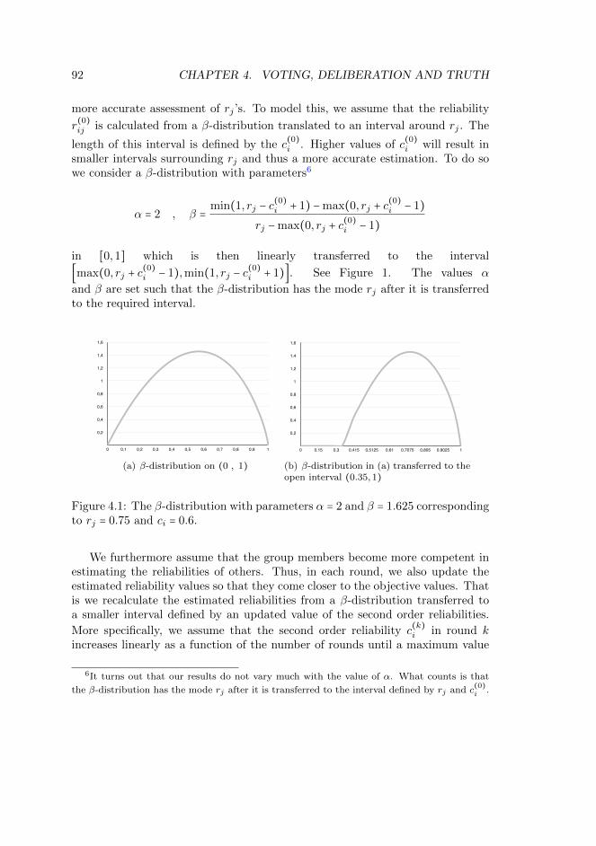
92 CHAPTER 4. VOTING, DELIBERATION AND TRUTH
more accurate assessment of rj ’s. To model this, we assume that the reliability
r(0)ij is calculated from a β-distribution translated to an interval around rj . The
length of this interval is defined by the c(0)i . Higher values of c
(0)i will result in
smaller intervals surrounding rj and thus a more accurate estimation. To do sowe consider a β-distribution with parameters6
α = 2 , β =min(1, rj − c
(0)i + 1) −max(0, rj + c
(0)i − 1)
rj −max(0, rj + c(0)i − 1)
in [0,1] which is then linearly transferred to the interval
[max(0, rj + c(0)i − 1),min(1, rj − c
(0)i + 1)]. See Figure 1. The values α
and β are set such that the β-distribution has the mode rj after it is transferredto the required interval.
Table 1
0 0 0
0,01 0,04776360944 1
0,02 0,0948026102 2
0,03 0,141114226
0,04 0,1866956326
0,05 0,2315439569
0,06 0,275656275
0,07 0,3190296107
0,08 0,361660934
0,09 0,403547161
0,1 0,4446851479
0,11 0,4850716943
0,12 0,524703538
0,13 0,563577355
0,14 0,601689755
0,15 0,639037282
0,16 0,67561641
0,17 0,711423543
0,18 0,746455009
0,19 0,780707062
0,2 0,814175873
0,21 0,846857534
0,22 0,878748052
0,23 0,909843344
0,24 0,940139237
0,25 0,969631462
0,26 0,998315652
0,27 1,026187338
0,28 1,053241944
0,29 1,079474784
0,3 1,104881056
0,31 1,129455838
0,32 1,153194083
0,33 1,176090615
0,34 1,198140121
0,35 1,219337146
0,36 1,239676087
0,37 1,259151185
0,38 1,277756522
0,39 1,295486005
0,4 1,312333368
0,41 1,328292156
0,42 1,343355718
0,43 1,357517197
0,44 1,370769521
0,45 1,383105389
0,46 1,39451726
0,47 1,404997342
0,48 1,414537573
0,49 1,423129609
0,5 1,43076481
0,51 1,437434217
0,52 1,443128535
0,53 1,447838115
0,54 1,451552928
0,55 1,45426254
0,56 1,455956088
0,57 1,456622251
0,58 1,456249214
0,59 1,454824636
0,6 1,452335611
0,61 1,448768627
0,62 1,444109515
0,63 1,4383434
0,64 1,431454645
0,65 1,42342678
0,66 1,41424244
0,67 1,403883275
0,68 1,392329866
0,69 1,37956162
0,7 1,365556656
0,71 1,350291674
0,72 1,3337418
0,73 1,315880423
0,74 1,296678988
0,75 1,276106769
0,76 1,254130605
0,77 1,230714577
0,78 1,205819647
0,79 1,179403208
0,8 1,151418562
0,81 1,121814275
0,82 1,090533406
0,83 1,05751254
0,84 1,022680595
0,85 0,985957313
0,86 0,947251323
0,87 0,906457631
0,88 0,863454285
0,89 0,818097872
0,9 0,770217269
0,91 0,719604743
0,92 0,666002808
0,93 0,609084042
0,94 0,548418421
0,95 0,4834169245
0,96 0,413225362
0,97 0,336498721
0,98 0,2508241302
0,99 0,1506627663
1 0
0,2
0,4
0,6
0,8
1
1,2
1,4
1,6
0 0,1 0,2 0,3 0,4 0,5 0,6 0,7 0,8 0,9 1
(a) β-distribution on (0 , 1)
Table 1
0 0 0
0,01 0,01 0
0,02 0,02 0
0,03 0,03 0
0,04 0,04 0
0,05 0,05 0
0,06 0,06 0
0,07 0,07 0
0,08 0,08 0
0,09 0,09 0
0,1 0,1 0
0,11 0,11 0
0,12 0,12 0
0,13 0,13 0
0,14 0,14 0
0,15 0,15 0
0,16 0,16 0
0,17 0,17 0
0,18 0,18 0
0,19 0,19 0
0,2 0,2 0
0,21 0,21 0
0,22 0,22 0
0,23 0,23 0
0,24 0,24 0
0,25 0,25 0
0,26 0,26 0
0,27 0,27 0
0,28 0,28 0
0,29 0,29 0
0,3 0,3 0
0,31 0,31 0
0,32 0,32 0
0,33 0,33 0
0,34 0,34 0
0,35 0,35 0
0,36 0,3565 0,04776360944
0,37 0,363 0,0948026102
0,38 0,3695 0,141114226
0,39 0,376 0,1866956326
0,4 0,3825 0,2315439569
0,41 0,389 0,275656275
0,42 0,3955 0,3190296107
0,43 0,402 0,361660934
0,44 0,4085 0,403547161
0,45 0,415 0,4446851479
0,46 0,4215 0,4850716943
0,47 0,428 0,524703538
0,48 0,4345 0,563577355
0,49 0,441 0,601689755
0,5 0,4475 0,639037282
0,51 0,454 0,67561641
0,52 0,4605 0,711423543
0,53 0,467 0,746455009
0,54 0,4735 0,780707062
0,55 0,48 0,814175873
0,56 0,4865 0,846857534
0,57 0,493 0,878748052
0,58 0,4995 0,909843344
0,59 0,506 0,940139237
0,6 0,5125 0,969631462
0,61 0,519 0,998315652
0,62 0,5255 1,026187338
0,63 0,532 1,053241944
0,64 0,5385 1,079474784
0,65 0,545 1,104881056
0,66 0,5515 1,129455838
0,67 0,558 1,153194083
0,68 0,5645 1,176090615
0,69 0,571 1,198140121
0,7 0,5775 1,219337146
0,71 0,584 1,239676087
0,72 0,5905 1,259151185
0,73 0,597 1,277756522
0,74 0,6035 1,295486005
0,75 0,61 1,312333368
0,76 0,6165 1,328292156
0,77 0,623 1,343355718
0,78 0,6295 1,357517197
0,79 0,636 1,370769521
0,8 0,6425 1,383105389
0,81 0,649 1,39451726
0,82 0,6555 1,404997342
0,83 0,662 1,414537573
0,84 0,6685 1,423129609
0,85 0,675 1,43076481
0,86 0,6815 1,437434217
0,87 0,688 1,443128535
0,88 0,6945 1,447838115
0,89 0,701 1,451552928
0,9 0,7075 1,45426254
0,91 0,714 1,455956088
0,92 0,7205 1,456622251
0,93 0,727 1,456249214
0,94 0,7335 1,454824636
0,95 0,74 1,452335611
0,96 0,7465 1,448768627
0,97 0,753 1,444109515
0,98 0,7595 1,4383434
0,99 0,766 1,431454645
1 0,7725 1,42342678
0,779 1,41424244
0,7855 1,403883275
0,792 1,392329866
0,7985 1,37956162
0,805 1,365556656
0,8115 1,350291674
0,818 1,3337418
0,8245 1,315880423
0,831 1,296678988
0,8375 1,276106769
0,844 1,254130605
0,8505 1,230714577
0,857 1,205819647
0,8635 1,179403208
0,87 1,151418562
0,8765 1,121814275
0,883 1,090533406
0,8895 1,05751254
0,896 1,022680595
0,9025 0,985957313
0,909 0,947251323
0,9155 0,906457631
0,922 0,863454285
0,9285 0,818097872
0,935 0,770217269
0,9415 0,719604743
0,948 0,666002808
0,9545 0,609084042
0,961 0,548418421
0,9675 0,4834169245
0,974 0,413225362
0,9805 0,336498721
0,987 0,2508241302
0,9935 0,1506627663
1 0
0,2
0,4
0,6
0,8
1
1,2
1,4
1,6
0 0,15 0,3 0,415 0,5125 0,61 0,7075 0,805 0,9025 1
(b) β-distribution in (a) transferred to theopen interval (0.35,1)
Figure 4.1: The β-distribution with parameters α = 2 and β = 1.625 correspondingto rj = 0.75 and ci = 0.6.
We furthermore assume that the group members become more competent inestimating the reliabilities of others. Thus, in each round, we also update theestimated reliability values so that they come closer to the objective values. Thatis we recalculate the estimated reliabilities from a β-distribution transferred toa smaller interval defined by an updated value of the second order reliabilities.
More specifically, we assume that the second order reliability c(k)i in round k
increases linearly as a function of the number of rounds until a maximum value
6It turns out that our results do not vary much with the value of α. What counts is that
the β-distribution has the mode rj after it is transferred to the interval defined by rj and c(0)i .
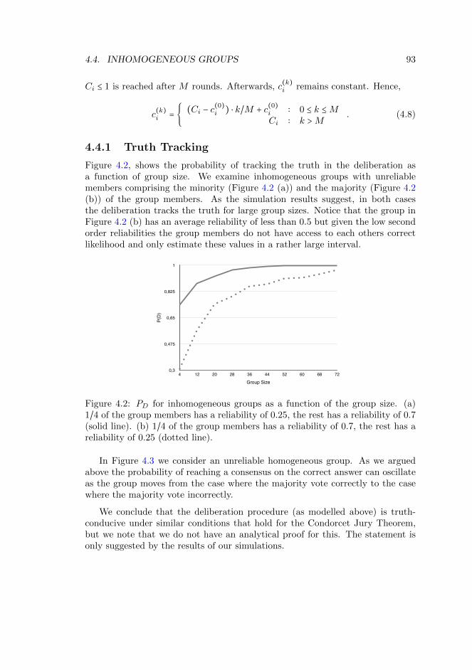
4.4. INHOMOGENEOUS GROUPS 93
Ci ≤ 1 is reached after M rounds. Afterwards, c(k)i remains constant. Hence,
c(k)i = {
(Ci − c(0)i ) ⋅ k/M + c
(0)i ∶ 0 ≤ k ≤MCi ∶ k >M
. (4.8)
4.4.1 Truth Tracking
Figure 4.2, shows the probability of tracking the truth in the deliberation asa function of group size. We examine inhomogeneous groups with unreliablemembers comprising the minority (Figure 4.2 (a)) and the majority (Figure 4.2(b)) of the group members. As the simulation results suggest, in both casesthe deliberation tracks the truth for large group sizes. Notice that the group inFigure 4.2 (b) has an average reliability of less than 0.5 but given the low secondorder reliabilities the group members do not have access to each others correctlikelihood and only estimate these values in a rather large interval.
4 0,30934 0,738612 0,56735 0,876820 0,73978 0,925928 0,79285 0,967436 0,86048 0,983244 0,87408 0,991752 0,9124 0,995660 0,91795 0,998168 0,94164 0,998972 0,96834 0,9993
P(D
)
0,3
0,475
0,65
0,825
1
Group Size4 12 20 28 36 44 52 60 68 72
Figure 4.2: PD for inhomogeneous groups as a function of the group size. (a)1/4 of the group members has a reliability of 0.25, the rest has a reliability of 0.7(solid line). (b) 1/4 of the group members has a reliability of 0.7, the rest has areliability of 0.25 (dotted line).
In Figure 4.3 we consider an unreliable homogeneous group. As we arguedabove the probability of reaching a consensus on the correct answer can oscillateas the group moves from the case where the majority vote correctly to the casewhere the majority vote incorrectly.
We conclude that the deliberation procedure (as modelled above) is truth-conducive under similar conditions that hold for the Condorcet Jury Theorem,but we note that we do not have an analytical proof for this. The statement isonly suggested by the results of our simulations.
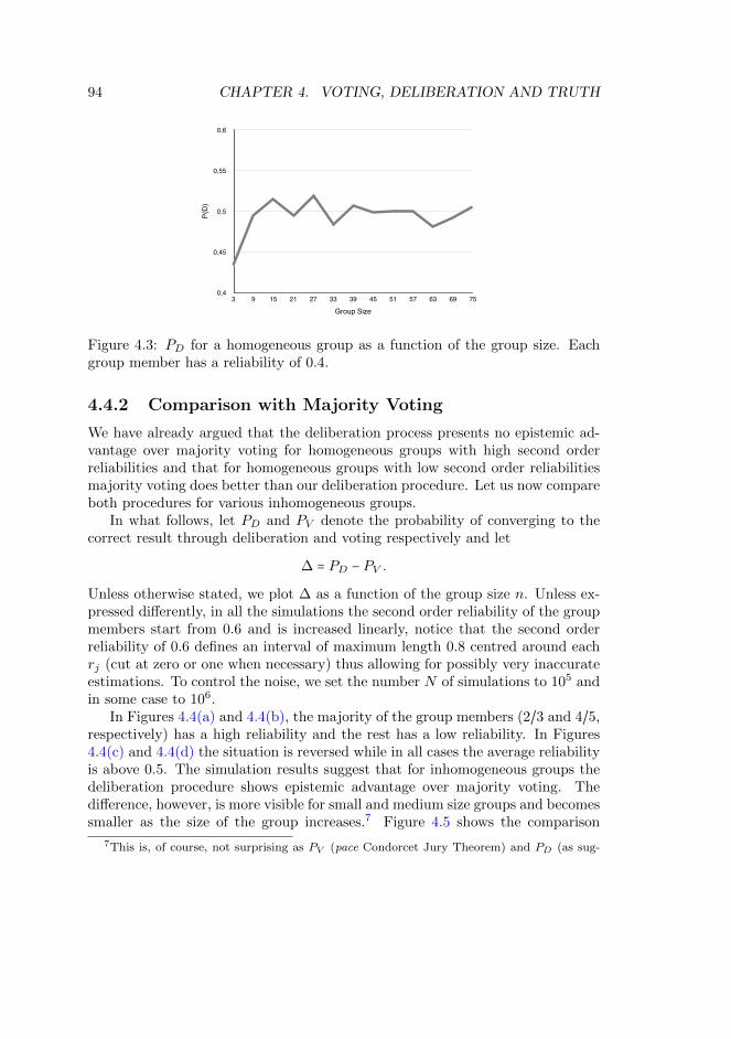
94 CHAPTER 4. VOTING, DELIBERATION AND TRUTH3 0,43350
9 0,49413
15 0,51484
21 0,49421
27 0,51921
33 0,48380
39 0,50720
45 0,49930
51 0,49987
57 0,49994
63 0,48064
69 0,4922
75 0,506
P(D
)
0,4
0,45
0,5
0,55
0,6
Group Size3 9 15 21 27 33 39 45 51 57 63 69 75
Figure 4.3: PD for a homogeneous group as a function of the group size. Eachgroup member has a reliability of 0.4.
4.4.2 Comparison with Majority Voting
We have already argued that the deliberation process presents no epistemic ad-vantage over majority voting for homogeneous groups with high second orderreliabilities and that for homogeneous groups with low second order reliabilitiesmajority voting does better than our deliberation procedure. Let us now compareboth procedures for various inhomogeneous groups.
In what follows, let PD and PV denote the probability of converging to thecorrect result through deliberation and voting respectively and let
∆ = PD − PV .
Unless otherwise stated, we plot ∆ as a function of the group size n. Unless ex-pressed differently, in all the simulations the second order reliability of the groupmembers start from 0.6 and is increased linearly, notice that the second orderreliability of 0.6 defines an interval of maximum length 0.8 centred around eachrj (cut at zero or one when necessary) thus allowing for possibly very inaccurateestimations. To control the noise, we set the number N of simulations to 105 andin some case to 106.
In Figures 4.4(a) and 4.4(b), the majority of the group members (2/3 and 4/5,respectively) has a high reliability and the rest has a low reliability. In Figures4.4(c) and 4.4(d) the situation is reversed while in all cases the average reliabilityis above 0.5. The simulation results suggest that for inhomogeneous groups thedeliberation procedure shows epistemic advantage over majority voting. Thedifference, however, is more visible for small and medium size groups and becomessmaller as the size of the group increases.7 Figure 4.5 shows the comparison
7This is, of course, not surprising as PV (pace Condorcet Jury Theorem) and PD (as sug-
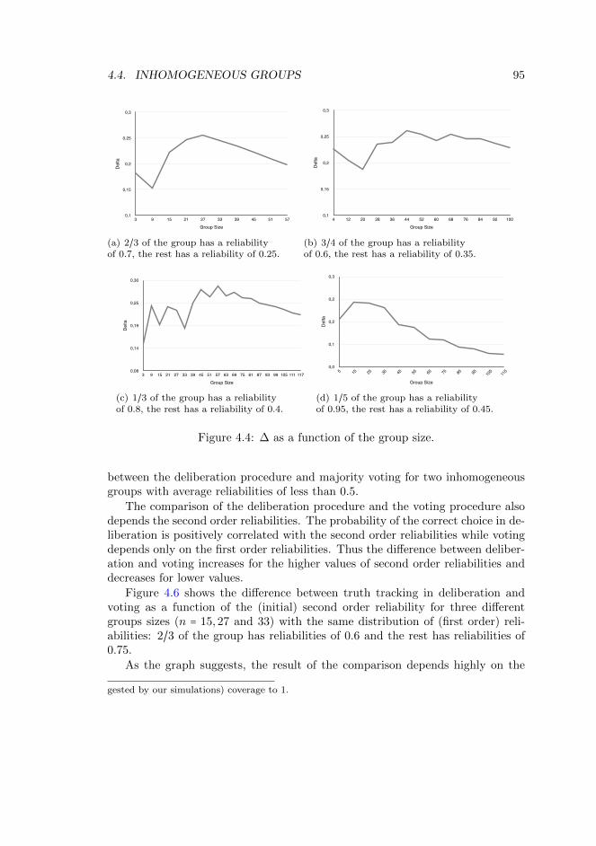
4.4. INHOMOGENEOUS GROUPS 953 0,77803 0,595828 0,1822029 0,78997 0,636998 0,152972
15 0,89446 0,671633 0,22282721 0,94635 0,699092 0,24725827 0,97734 0,721088 0,25625233 0,98612 0,740232 0,24588839 0,99309 0,757802 0,23528845 0,99634 0,773328 0,22301251 0,99780 0,787741 0,21005957 0,99852 0,800211 0,198309
Del
ta
0,1
0,15
0,2
0,25
0,3
Group Size3 9 15 21 27 33 39 45 51 57
(a) 2/3 of the group has a reliabilityof 0.7, the rest has a reliability of 0.25.
4 0.59459 0,367841 0,226749 0,182202
12 0,695310 0,490974 0,204336 0,15297220 0,736040 0,548633 0,187407 0,22282728 0,822240 0,586388 0,235852 0,24725836 0,856050 0,616286 0,239764 0,25625244 0,902520 0,641361 0,261159 0,24588852 0,914720 0,660980 0,253740 0,23528860 0,922820 0,679639 0,243181 0,22301268 0,950990 0,696719 0,254271 0,21005976 0,957870 0,711370 0,246500 0,19830984 0,24608792 0,236531
100 0,229288
Del
ta
0,1
0,15
0,2
0,25
0,3
Group Size4 12 20 28 36 44 52 60 68 76 84 92 100
(b) 3/4 of the group has a reliabilityof 0.6, the rest has a reliability of 0.35.
3 0,1469 0,237
15 0,19221 0,23627 0,22633 0,18339 0,24545 0,27751 0,26057 0,28563 0,26269 0,27175 0,25681 0,25587 0,24593 0,24199 0,235
105 0,230111 0,221117 0,216
Del
ta
0,08
0,14
0,19
0,25
0,30
Group Size3 9 15 21 27 33 39 45 51 57 63 69 75 81 87 93 99 105 111 117
(c) 1/3 of the group has a reliabilityof 0.8, the rest has a reliability of 0.4.
5 0,157
15 0,216
25 0,213
35 0,197
45 0,139
55 0,130
65 0,093
75 0,089
85 0,065
95 0,060
105 0,044
115 0,040 Del
ta
0,0
0,1
0,2
0,2
0,3
Group Size
5 15 25 35 45 55 65 75 85 95 105
115
(d) 1/5 of the group has a reliabilityof 0.95, the rest has a reliability of 0.45.
Figure 4.4: ∆ as a function of the group size.
between the deliberation procedure and majority voting for two inhomogeneousgroups with average reliabilities of less than 0.5.
The comparison of the deliberation procedure and the voting procedure alsodepends the second order reliabilities. The probability of the correct choice in de-liberation is positively correlated with the second order reliabilities while votingdepends only on the first order reliabilities. Thus the difference between deliber-ation and voting increases for the higher values of second order reliabilities anddecreases for lower values.
Figure 4.6 shows the difference between truth tracking in deliberation andvoting as a function of the (initial) second order reliability for three differentgroups sizes (n = 15,27 and 33) with the same distribution of (first order) reli-abilities: 2/3 of the group has reliabilities of 0.6 and the rest has reliabilities of0.75.
As the graph suggests, the result of the comparison depends highly on the
gested by our simulations) coverage to 1.
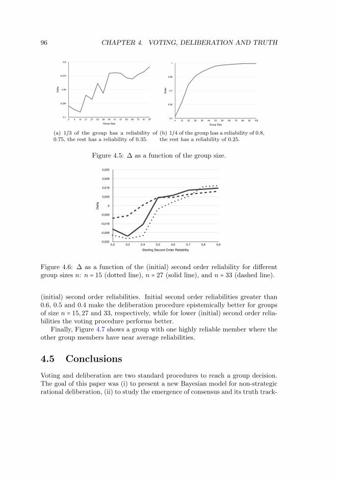
96 CHAPTER 4. VOTING, DELIBERATION AND TRUTH3 0,66521 0,464097 0,2011139 0,62227 0,452889 0,169381
15 0,58783 0,440956 0,14687421 0,73214 0,432373 0,29976727 0,68701 0,424692 0,26231833 0,82287 0,416261 0,40660939 0,72491 0,408826 0,31608445 0,89792 0,402465 0,49545551 0,90235 0,397941 0,50440957 0,88926 0,390693 0,49856763 0,84092 0,386384 0,45453669 0.82848 0,381666 0,44681475 0,86518 0,376514 0,48866681 0,88433 0,372091 0,51223987 0,92769 0,36815 0,559540
Del
ta
0,1
0,225
0,35
0,475
0,6
Group Size3 9 15 21 27 33 39 45 51 57 63 69 75 81 87
(a) 1/3 of the group has a reliability of0.75, the rest has a reliability of 0.35.
4 0,54863 0,128495 0,42013512 0,67676 0,104787 0,57197320 0,84137 0,07576 0,76561028 0,91424 0,054445 0,85979536 0,94318 0,039295 0,90388544 0,9688 0,028517 0,94028352 0,985 0,020897 0,96410360 0,99196 0,015234 0,97672668 0,99629 0,011139 0,98515176 0,99833 0,008172 0,99015884 0,99902 0,006123 0,99289792 0,9996 0,004395 0,995205
100 0,9999 0,003401 0,996499
Del
ta
0,4
0,55
0,7
0,85
1
Group Size4 12 20 28 36 44 52 60 68 76 84 92 100
(b) 1/4 of the group has a reliability of 0.8,the rest has a reliability of 0.25.
Figure 4.5: ∆ as a function of the group size.0,2 -0,098098 -0,0284799999999999-0,022834 -0,0123110,3 -0,16324 -0,032344 -0,029571 -0,009603999999999950,4 -0,06212 -0,028922 -0,01801 0,0006509999999999570,5 -0,0199330000000001-0,003195999999999980,007355 0,008032000000000040,6 -0,02057 0,003848000000000070,009950000000000010,008203000000000070,7 0,006881000000000030,009012999999999940,01516999999999990,0109450,8 0,015117 0,01849899999999990,015996 0,01240,9 0,01338000000000010,019267 0,01684700000000010,0139359999999999
Delta
-0,035
-0,026
-0,018
-0,009
0
0,009
0,018
0,026
0,035
Starting Second Order Reliability0,2 0,3 0,4 0,5 0,6 0,7 0,8 0,9
Figure 4.6: ∆ as a function of the (initial) second order reliability for differentgroup sizes n: n = 15 (dotted line), n = 27 (solid line), and n = 33 (dashed line).
(initial) second order reliabilities. Initial second order reliabilities greater than0.6, 0.5 and 0.4 make the deliberation procedure epistemically better for groupsof size n = 15,27 and 33, respectively, while for lower (initial) second order relia-bilities the voting procedure performs better.
Finally, Figure 4.7 shows a group with one highly reliable member where theother group members have near average reliabilities.
4.5 Conclusions
Voting and deliberation are two standard procedures to reach a group decision.The goal of this paper was (i) to present a new Bayesian model for non-strategicrational deliberation, (ii) to study the emergence of consensus and its truth track-
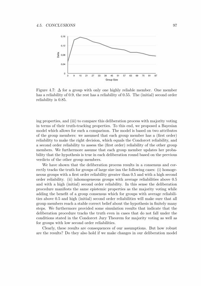
4.5. CONCLUSIONS 97
3 0,05029 0,1441
15 0,156021 0,150427 0,136333 0,130439 0,120045 0,109351 0,105557 0,101163 0,090769 0,090575 0,085281 0,077787 0,0756
Del
ta
0
0,04
0,08
0,12
0,16
Group Size3 9 15 21 27 33 39 45 51 57 63 69 75 81 87
Figure 4.7: ∆ for a group with only one highly reliable member. One memberhas a reliability of 0.9, the rest has a reliability of 0.55. The (initial) second orderreliability is 0.85.
ing properties, and (iii) to compare this deliberation process with majority votingin terms of their truth-tracking properties. To this end, we proposed a Bayesianmodel which allows for such a comparison. The model is based on two attributesof the group members: we assumed that each group member has a (first order)reliability to make the right decision, which equals the Condorcet reliability, anda second order reliability to assess the (first order) reliability of the other groupmembers. We furthermore assume that each group member updates her proba-bility that the hypothesis is true in each deliberation round based on the previousverdicts of the other group members.
We have shown that the deliberation process results in a consensus and cor-rectly tracks the truth for groups of large size inn the following cases: (i) homoge-neous groups with a first order reliability greater than 0.5 and with a high secondorder reliability. (ii) inhomogeneous groups with average reliabilities above 0.5and with a high (initial) second order reliability. In this sense the deliberationprocedure manifests the same epistemic properties as the majority voting whileadding the benefit of a group consensus which for groups with average reliabili-ties above 0.5 and high (initial) second order reliabilities will make sure that allgroup members reach a stable correct belief about the hypothesis in finitely manysteps. We furthermore provided some simulation results that indicate that thedeliberation procedure tracks the truth even in cases that do not fall under theconditions stated in the Condorcet Jury Theorem for majority voting as well asfor groups with low second order reliabilities.
Clearly, these results are consequences of our assumptions. But how robustare the results? Do they also hold if we make changes in our deliberation model
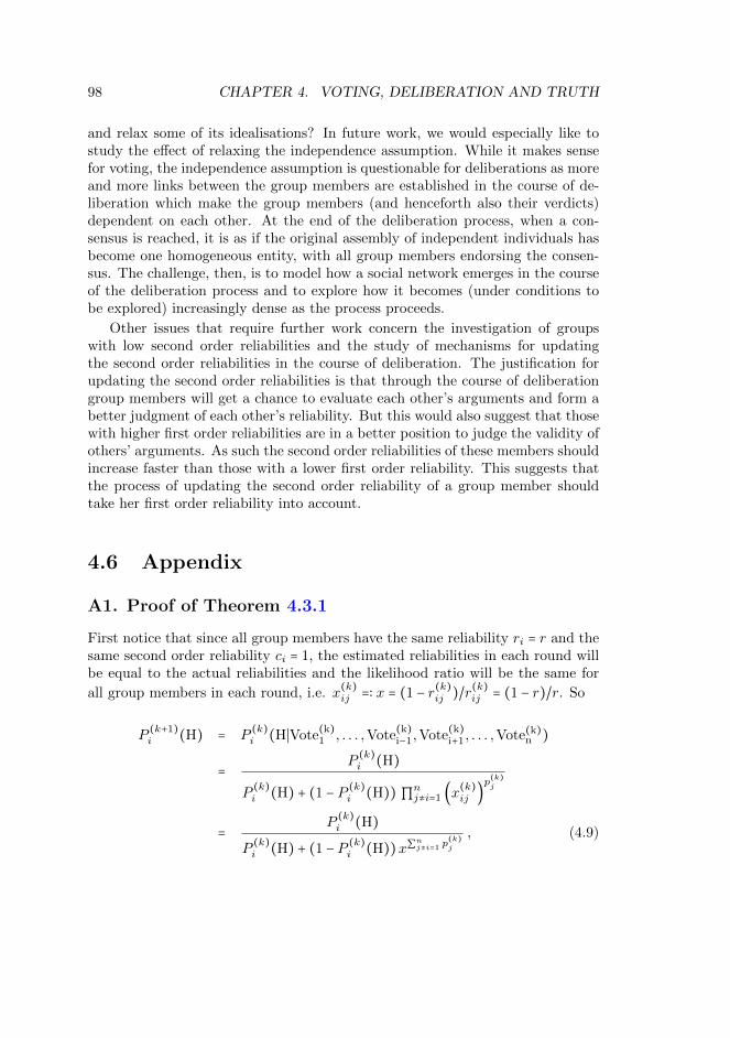
98 CHAPTER 4. VOTING, DELIBERATION AND TRUTH
and relax some of its idealisations? In future work, we would especially like tostudy the effect of relaxing the independence assumption. While it makes sensefor voting, the independence assumption is questionable for deliberations as moreand more links between the group members are established in the course of de-liberation which make the group members (and henceforth also their verdicts)dependent on each other. At the end of the deliberation process, when a con-sensus is reached, it is as if the original assembly of independent individuals hasbecome one homogeneous entity, with all group members endorsing the consen-sus. The challenge, then, is to model how a social network emerges in the courseof the deliberation process and to explore how it becomes (under conditions tobe explored) increasingly dense as the process proceeds.
Other issues that require further work concern the investigation of groupswith low second order reliabilities and the study of mechanisms for updatingthe second order reliabilities in the course of deliberation. The justification forupdating the second order reliabilities is that through the course of deliberationgroup members will get a chance to evaluate each other’s arguments and form abetter judgment of each other’s reliability. But this would also suggest that thosewith higher first order reliabilities are in a better position to judge the validity ofothers’ arguments. As such the second order reliabilities of these members shouldincrease faster than those with a lower first order reliability. This suggests thatthe process of updating the second order reliability of a group member shouldtake her first order reliability into account.
4.6 Appendix
A1. Proof of Theorem 4.3.1
First notice that since all group members have the same reliability ri = r and thesame second order reliability ci = 1, the estimated reliabilities in each round willbe equal to the actual reliabilities and the likelihood ratio will be the same for
all group members in each round, i.e. x(k)ij =∶ x = (1 − r
(k)ij )/r
(k)ij = (1 − r)/r. So
P(k+1)i (H) = P
(k)i (H∣Vote
(k)1 , . . . ,Vote
(k)i−1,Vote
(k)i+1, . . . ,Vote(k)n )
=P(k)i (H)
P(k)i (H) + (1 − P
(k)i (H)) ∏
nj≠i=1 (x
(k)ij )
p(k)j
=P(k)i (H)
P(k)i (H) + (1 − P
(k)i (H))x∑
nj≠i=1 p
(k)j
, (4.9)
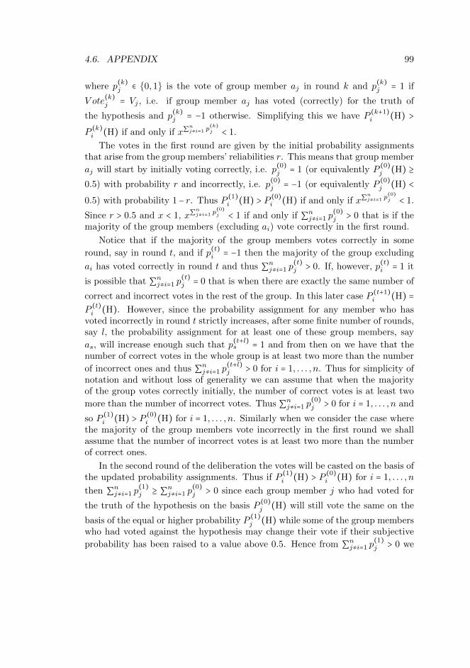
4.6. APPENDIX 99
where p(k)j ∈ {0,1} is the vote of group member aj in round k and p
(k)j = 1 if
V ote(k)j = Vj , i.e. if group member aj has voted (correctly) for the truth of
the hypothesis and p(k)j = −1 otherwise. Simplifying this we have P
(k+1)i (H) >
P(k)i (H) if and only if x∑
nj≠i=1 p
(k)j < 1.
The votes in the first round are given by the initial probability assignmentsthat arise from the group members’ reliabilities r. This means that group member
aj will start by initially voting correctly, i.e. p(0)j = 1 (or equivalently P
(0)j (H) ≥
0.5) with probability r and incorrectly, i.e. p(0)j = −1 (or equivalently P
(0)j (H) <
0.5) with probability 1− r. Thus P(1)i (H) > P
(0)i (H) if and only if x∑
nj≠i=1 p
(0)j < 1.
Since r > 0.5 and x < 1, x∑nj≠i=1 p
(0)j < 1 if and only if ∑
nj≠i=1 p
(0)j > 0 that is if the
majority of the group members (excluding ai) vote correctly in the first round.
Notice that if the majority of the group members votes correctly in some
round, say in round t, and if p(t)i = −1 then the majority of the group excluding
ai has voted correctly in round t and thus ∑nj≠i=1 p
(t)j > 0. If, however, p
(t)i = 1 it
is possible that ∑nj≠i=1 p
(t)j = 0 that is when there are exactly the same number of
correct and incorrect votes in the rest of the group. In this later case P(t+1)i (H) =
P(t)i (H). However, since the probability assignment for any member who has
voted incorrectly in round t strictly increases, after some finite number of rounds,say l, the probability assignment for at least one of these group members, say
as, will increase enough such that p(t+l)s = 1 and from then on we have that the
number of correct votes in the whole group is at least two more than the number
of incorrect ones and thus ∑nj≠i=1 p
(t+l)j > 0 for i = 1, . . . , n. Thus for simplicity of
notation and without loss of generality we can assume that when the majorityof the group votes correctly initially, the number of correct votes is at least two
more than the number of incorrect votes. Thus ∑nj≠i=1 p
(0)j > 0 for i = 1, . . . , n and
so P(1)i (H) > P
(0)i (H) for i = 1, . . . , n. Similarly when we consider the case where
the majority of the group members vote incorrectly in the first round we shallassume that the number of incorrect votes is at least two more than the numberof correct ones.
In the second round of the deliberation the votes will be casted on the basis ofthe updated probability assignments. Thus if P
(1)i (H) > P
(0)i (H) for i = 1, . . . , n
then ∑nj≠i=1 p
(1)j ≥ ∑
nj≠i=1 p
(0)j > 0 since each group member j who had voted for
the truth of the hypothesis on the basis P(0)j (H) will still vote the same on the
basis of the equal or higher probability P(1)j (H) while some of the group members
who had voted against the hypothesis may change their vote if their subjective
probability has been raised to a value above 0.5. Hence from ∑nj≠i=1 p
(1)j > 0 we
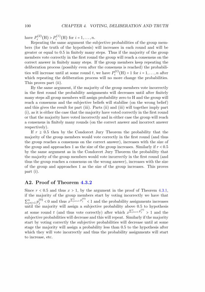
100 CHAPTER 4. VOTING, DELIBERATION AND TRUTH
have P(2)i (H) > P
(1)i (H) for i = 1, . . . , n.
Repeating the same argument the subjective probabilities of the group mem-bers (for the truth of the hypothesis) will increases in each round and will begreater or equal to 0.5 in finitely many steps. Thus if the majority of the groupmembers vote correctly in the first round the group will reach a consensus on thecorrect answer in finitely many steps. If the group members keep repeating thedeliberation process (possibly even after the consensus is reached) the probabili-
ties will increase until at some round t, we have P(t)i (H) = 1 for i = 1, . . . , n after
which repeating the deliberation process will no more change the probabilities.This proves part (ii).
By the same argument, if the majority of the group members vote incorrectlyin the first round the probability assignments will decreases until after finitelymany steps all group members will assign probability zero to H and the group willreach a consensus and the subjective beliefs will stabilise (on the wrong belief)and this gives the result for part (iii). Parts (ii) and (iii) will together imply part(i), as it is either the case that the majority have voted correctly in the first roundor that the majority have voted incorrectly and in either case the group will reacha consensus in finitely many rounds (on the correct answer and incorrect answerrespectively).
If r ≥ 0.5 then by the Condorcet Jury Theorem the probability that themajority of the group members would vote correctly in the first round (and thusthe group reaches a consensus on the correct answer), increases with the size ofthe group and approaches 1 as the size of the group increases. Similarly if r < 0.5by the same argument as in the Condorcet Jury Theorem the probability thatthe majority of the group members would vote incorrectly in the first round (andthus the group reaches a consensus on the wrong answer), increases with the sizeof the group and approaches 1 as the size of the group increases. This provespart (i).
A2. Proof of Theorem 4.3.2
Since r < 0.5 and thus x > 1, by the argument in the proof of Theorem 4.3.1,if the majority of the group members start by voting incorrectly we have that
∑nj≠i=1 p
(0)j < 0 and thus x∑
nj≠i=1 p
(0)j < 1 and the probability assignments increases
until the majority will assign a subjective probability above 0.5 to hypothesis
at some round t (and thus vote correctly) after which x∑nj≠i=1 p
(t)j > 1 and the
subjective probabilities will decrease and this will repeat. Similarly if the majoritystart by voting correctly the subjective probabilities will decrease until at somestage the majority will assign a probability less than 0.5 to the hypothesis afterwhich they will vote incorrectly and thus the probability assignments will startto increase, etc.
Chapter 5
Anchoring In Deliberations
5.1 Introduction
There are numerous instances of group decision making in everyday practice.Families have to decide where to go on holiday, funding agencies have to decidewhich research projects to support, and juries in court have to decide whether adefendant is guilty or not. Sometimes a decision is made in the light of differentpreferences (and each group member wants to get the best out for herself), andsometimes all group members share the conviction that the resulting decisionshould be best in some sense that is commonly agreed upon. Juries in court, forexample, want to make the right decision. Everybody wants that a guilty per-son is convicted, and no one wants that an innocent is sent to prison. Likewise,committees such as the IPPC deliberate to arrive at the best far-reaching policyrecommendations.
There are many different ways that a group can make such decisions. Whendeciding in light of different preferences, for example, the goal is naturally tominimise the average compromise and leave the decision makers as happy as pos-sible with the final decision and when deciding toward some objective truth thegoal is to approximate the correct decision as close as possible. Different decisionmaking process are, thus, chosen based on which characteristics they manifestthe best.
Deliberation is one extensively practiced approach to decision making in bothsuch scenarios. It provides an advantage of allowing the decision makers to reviseand change their opinion and thus stabilising a dynamics that can ideally leadthe group to a collective consensus on which the group agrees as a unanimousentity. This is indeed a sought after characteristic for a group decision makingprocedure to leave all the participant in agreement and convinced of the final
101
102 CHAPTER 5. ANCHORING IN DELIBERATIONS
decision. On the other hand, the possibility of learning other opinions paves theway for easier recognition of mistakes and better availability of information whichhelp to better estimate the correct decision when such exists.
Adding the interactive component to the decision making, however, does alsointroduce a whole spectrum of other relevant factors, including those associatedwith the psychological aspects of social interactions. There are many factorsthat can affect how people influence each other in their interactions, from theway that one reacts to the opinions of those from different social, economicalor educational classes to the intricate and complex dynamics of power in socialnetworks. Phenomena resulting from such factors, including information cas-cades, pluralistic ignorance, anchoring, etc., have been studied by psychologistfor a rather long time to varying degrees. Some are well understood, analysedand agreed upon but most have proved hard to characterise in an uncontrover-sial way or even harder to do so in a manner exact enough to be account for intechnical formalisations. Nevertheless, there is an increasing tendency in socialscientists and psychologists toward development and adoption of formal models,and to our opinion, very rightly so.
This does not ,by any means, intended to suggest that we believe that thesubtlety of the psychological (and socio-psychological) phenomenons can be com-pletely and adequately captured in some mathematical and formal apparatus.Rather it is meant to emphasise on the fact that such formalisations, even withthe necessary idealisations and abstractions that are inevitable in devising formalmodels, can surface persisting patterns and trends and shed light on general char-acteristics, aspects, and correlations between the relevant factors to be studied inmore details (in possibly non-formal approaches). In this regard, the newly es-tablished links between the Bayesian Epistemology, as our best theory of gradedbelief, and the concepts in psychology (and socio-psychology) should be cele-brated and carefully attended.
One such psychological phenomenon that is relevant to interaction of groupmembers and the formation of a collective consensus is the anchoring effect. Thisis a social-psychological instance of an effect that is widely discussed in the heuris-tics and biases program in cognitive psychology, (Tversky & Kahneman 1974),(Kahneman et. al. 2006). In general anchoring is a cognitive bias that describesthe common human tendency to rely heavily on some (usually irrelevant) pieceof information when making decisions.
There are many different instances of anchoring effect arising even in an indi-vidual decision making. As it relates to the deliberation process, anchoring occurswhen the group consensus depends, for example, on the order in which the groupmembers present their views in the course of a deliberation. More specifically,the experiments suggest that the group member who speaks first will typicallyhave the highest impact on the decision on which the group eventually settles. In
5.2. MODELING ANCHORING 103
such cases the first speaker is said to have anchored the deliberation. The effectis particularly important for the epistemic analysis of the deliberation as it opensthe way to possible manipulation of the process and thus bears negatively on theepistemic characteristic of the final decision.
The reasons for the emergence of the anchoring effect are usually associatedwith what is known as the bounded rationality. These are the cognitive limita-tions of the decision makers including, short attention span, memory loss, looseof cognitive ability by fatigue, etc. That the effect can happen as a result ofsuch limitations seems clear. So the question we will ask here is whether or notsuch cognitive limitations are the only causes for this bias? In other words weask whether the anchoring effect can also occur in a group of truth-seeking, fullyrational members, who update their beliefs according to plausible rules, simplyas a result of the updating procedure.
To address this question, the remainder of this paper is organised as follows.We shall first proposes an incremental model for deliberation, inspired by thewell-known Lehrer-Wagner model in Section 5.2. Using this model, we study theanchoring effect in Section 5.3 and will conclude in Section 5.4.
5.2 Modeling Anchoring
To study the emergence of the anchoring effect, we will first need a formalisationof the deliberation process. There are several models of deliberation studied inthe literature including two Bayesian models developed by Angere and Olsson,(3), (Olsson 2011), and Hartmann and Rafiee Rad (Chapter 4). Both thesemodels, however, make a crucial independence assumption by which the order inwhich the evidence comes in will be inconsequential. Thus it will not be possibleto study the path-dependence of the deliberation process with these models.
Next are the Lehrer-Wagner model, (Lehrer 1976), (Lehrer & Wagner 1981),and Hegselmann-Krause model (Hegselmann & Krause 2002;Hegselmann & Krause 2006; Hegselmann & Krause 2009). The Lehrer-Wagnermodel is probably the most well known model in the literature for collectiveconsensus which focuses on deliberating groups that have to fix the value of areal-valued parameter. According to the model, each group member submitsher initial assignment and assigns normalised weights to all group members,including herself. The revised assignment of each group member will be theweighted average of all initial submissions using the assigned weights. It is nothard top show that, if the process is iterated, under rather weak conditions thevalues will converge. This model, however, assumes that all assignments in eachround are made simultaneously, and so again the supposed path-dependence ofthe deliberation cannot be accounted for in this model. The Hegselmann-Krausemodel has a similar problem. According to this model, each agent takes into
104 CHAPTER 5. ANCHORING IN DELIBERATIONS
account only those judgments that are sufficiently close to her own initialassignment and the updating procedure happens on the full profile of all suchopinions at the same time.
It is important to note, however, that these models are all intended asnormative models for rational deliberation developed in such a manner to avoidsuch biases as the anchoring. To study the emergence of this effect we will needa descriptive model for deliberation or one closer to how the actual deliberationsare carried out in groups. In real deliberations the group members are hardlyindependent, and even if they start as such, during the course of the deliberationdependencies will form and become more and more complicated as the processgoes on. It is also usually not the case that people would wait to hear all theopinions before updating theirs and every opinion and argument does leavesome influence as it is presented. We will next propose a simple formalisationof the deliberation process (a modified version of the Lehrer-Wagner model)that captures this intuition and allows fro the study of path-dependence indeliberation. As in the Lehrer-Wagner model we consider a group aiming toestimate the value of a real valued parameter x through deliberative process.The model works on the following premises:
• Each group member is assumed to have a first order reliability that cap-tures his competence in giving the correct judgement and a second orderreliability that captures his ability to estimate the competence of his fellowgroup members.
• Each group member estimates the reliability of her fellow group membersand use these estimated reliabilities to weight the opinions of others.
• The updating procedure proceeds in an incremental manner, that is, thegroup members update their opinion after each announcement. Thus eachround of deliberation in a group of n agents, consists of n steps. In eachstep a group member announces her opinion and everyone updates basedon this announcement.
• The way each group member updates her opinion depends on the reliabilitythat she assigns to speaker in relation to the reliability she assigns to herself.
• People’s ability to estimate the competence of others improve during thecourse of deliberation.
So here is the sketch of how the model works; Consider a group of n memberswho have to fix the value of a real-valued parameter x and let’s order the group
members from 1 to n. Initially, each group member i submits an initial value x(0)i
and fixes a value for the reliability of her judgment. In round 1, step 1, the first
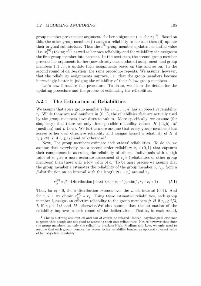
5.2. MODELING ANCHORING 105
group member presents her arguments for her assignment (i.e. for x(0)1 ). Based on
this, the other group members (i) assign a reliability to her and then (ii) updatetheir original submissions. Thus the ith group member updates her initial value
(i.e. x(0)i ) taking x
(0)1 as well as her own reliability and the reliability she assigns to
the first group member into account. In the next step, the second group memberpresents her arguments for her (now already once updated) assignment, and groupmembers 1,3, . . . , n update their assignments based on this and so on. In thesecond round of deliberation, the same procedure repeats. We assume, however,that the reliability assignments improve, i.e. that the group members becomeincreasingly better in judging the reliability of their fellow group members.
Let’s now formalise this procedure. To do so, we fill in the details for theupdating procedure and the process of estimating the reliabilities.
5.2.1 The Estimation of Reliabilities
We assume that every group member i (for i = 1, . . . , n) has an objective reliabilityri. While these are real numbers in (0,1), the reliabilities that are actually usedby the group members have discrete values. More specifically, we assume (forsimplicity) that there are only three possible reliability values: H (high), M(medium) and L (low). We furthermore assume that every group member i hasaccess to her own objective reliability and assigns herself a reliability of H ifri ≥ 2/3, L if ri ≤ 1/3 and M otherwise.1
Next, The group members estimate each others’ reliabilities. To do so, weassume that everybody has a second order reliability ci ∈ (0,1) that capturestheir competence in assessing the reliability of others. Individuals with a highvalue of ci give a more accurate assessment of rj ’s (reliabilities of other groupmembers) than those with a low value of ci. To be more precise we assume thatthe group member i estimates the reliability of the group member j, rij , from aβ-distribution on an interval with the length 2(1 − ci) around rj .
r(0)ij = β −Distribution [max(0, rj + ci − 1),min(1, rj − ci + 1)] (5.1)
Thus, for ci = 0, the β-distribution extends over the whole interval (0,1). And
for ci = 1, we obtain r(0)ij = rj . Using these estimated reliabilities, each group
member i, assigns an effective reliability to the group members j: H if rij ≥ 2/3,L if rij ≤ 1/3 and M otherwise.We also assume that the estimation of thereliability improve in each round of the deliberation. That is, in each round,
1 This is a strong assumption and can of course be relaxed. Indeed, psychological evidencesuggests that people are not good at assessing their own reliabilities. Notice however that sincethe group members use only the reliability brackets High, Medium and Low, we only need toassume that each group member has access to her reliability bracket as opposed to exact valueof her objective reliability.
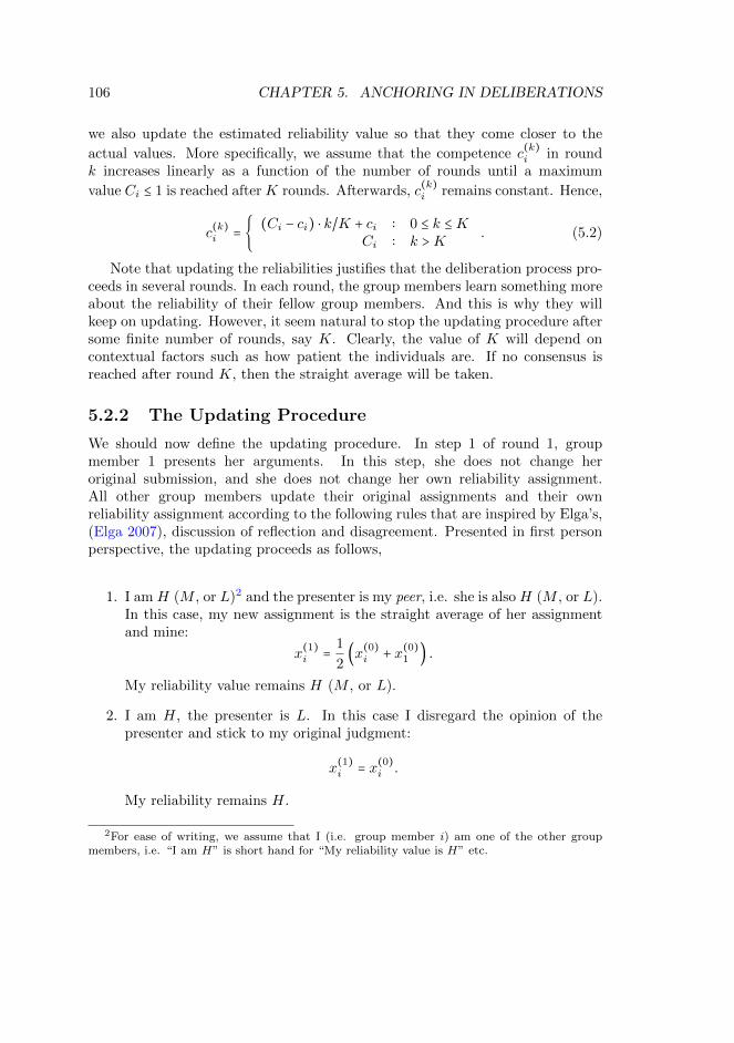
106 CHAPTER 5. ANCHORING IN DELIBERATIONS
we also update the estimated reliability value so that they come closer to the
actual values. More specifically, we assume that the competence c(k)i in round
k increases linearly as a function of the number of rounds until a maximum
value Ci ≤ 1 is reached after K rounds. Afterwards, c(k)i remains constant. Hence,
c(k)i = {
(Ci − ci) ⋅ k/K + ci ∶ 0 ≤ k ≤KCi ∶ k >K
. (5.2)
Note that updating the reliabilities justifies that the deliberation process pro-ceeds in several rounds. In each round, the group members learn something moreabout the reliability of their fellow group members. And this is why they willkeep on updating. However, it seem natural to stop the updating procedure aftersome finite number of rounds, say K. Clearly, the value of K will depend oncontextual factors such as how patient the individuals are. If no consensus isreached after round K, then the straight average will be taken.
5.2.2 The Updating Procedure
We should now define the updating procedure. In step 1 of round 1, groupmember 1 presents her arguments. In this step, she does not change heroriginal submission, and she does not change her own reliability assignment.All other group members update their original assignments and their ownreliability assignment according to the following rules that are inspired by Elga’s,(Elga 2007), discussion of reflection and disagreement. Presented in first personperspective, the updating proceeds as follows,
1. I am H (M , or L)2 and the presenter is my peer, i.e. she is also H (M , or L).In this case, my new assignment is the straight average of her assignmentand mine:
x(1)i =
1
2(x(0)i + x
(0)1 ) .
My reliability value remains H (M , or L).
2. I am H, the presenter is L. In this case I disregard the opinion of thepresenter and stick to my original judgment:
x(1)i = x
(0)i .
My reliability remains H.
2For ease of writing, we assume that I (i.e. group member i) am one of the other groupmembers, i.e. “I am H” is short hand for “My reliability value is H” etc.
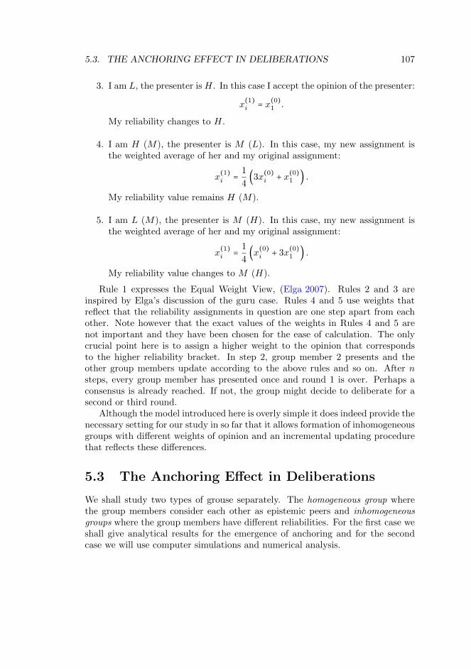
5.3. THE ANCHORING EFFECT IN DELIBERATIONS 107
3. I am L, the presenter is H. In this case I accept the opinion of the presenter:
x(1)i = x
(0)1 .
My reliability changes to H.
4. I am H (M), the presenter is M (L). In this case, my new assignment isthe weighted average of her and my original assignment:
x(1)i =
1
4(3x
(0)i + x
(0)1 ) .
My reliability value remains H (M).
5. I am L (M), the presenter is M (H). In this case, my new assignment isthe weighted average of her and my original assignment:
x(1)i =
1
4(x(0)i + 3x
(0)1 ) .
My reliability value changes to M (H).
Rule 1 expresses the Equal Weight View, (Elga 2007). Rules 2 and 3 areinspired by Elga’s discussion of the guru case. Rules 4 and 5 use weights thatreflect that the reliability assignments in question are one step apart from eachother. Note however that the exact values of the weights in Rules 4 and 5 arenot important and they have been chosen for the ease of calculation. The onlycrucial point here is to assign a higher weight to the opinion that correspondsto the higher reliability bracket. In step 2, group member 2 presents and theother group members update according to the above rules and so on. After nsteps, every group member has presented once and round 1 is over. Perhaps aconsensus is already reached. If not, the group might decide to deliberate for asecond or third round.
Although the model introduced here is overly simple it does indeed provide thenecessary setting for our study in so far that it allows formation of inhomogeneousgroups with different weights of opinion and an incremental updating procedurethat reflects these differences.
5.3 The Anchoring Effect in Deliberations
We shall study two types of grouse separately. The homogeneous group wherethe group members consider each other as epistemic peers and inhomogeneousgroups where the group members have different reliabilities. For the first case weshall give analytical results for the emergence of anchoring and for the secondcase we will use computer simulations and numerical analysis.
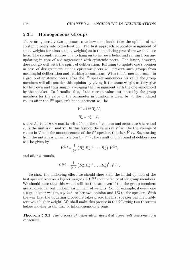
108 CHAPTER 5. ANCHORING IN DELIBERATIONS
5.3.1 Homogeneous Groups
There are generally two approaches to how one should take the opinion of herepistemic peers into consideration. The first approach advocates assignment ofequal weights (or almost equal weights) as in the updating procedure we shall usehere. The second, requires one to hang on to her own belief and refrain from anyupdating in case of a disagreement with epistemic peers. The latter, however,does not go well with the spirit of deliberation. Refusing to update one’s opinionin case of disagreement among epistemic peers will prevent such groups frommeaningful deliberation and reaching a consensus. With the former approach, ina group of epistemic peers, after the ith speaker announces his value the groupmembers will all consider this opinion by giving it the same weight as they giveto their own and thus simply averaging their assignment with the one announcedby the speaker. To formalise this, if the current values estimated by the groupmembers for the value of the parameter in question is given by V , the updatedvalues after the ith speaker’s announcement will be
V ′ = 1/2Bin.V ,
Bin = Ain + In,
where Ain is an n×n matrix with 1’s on the ith column and zeros else where andIn is the unit n×n matrix. In this fashion the values in V ′ will be the average ofvalues in V and the announcement of the ith speaker, that is < V >i. So, startingfrom the initial assignments given by V (0), the result of one round of deliberationwill be given by
V (1) =1
2n(Bnn .B
n−1n . . . . .B1
n) .V(0),
and after k rounds,
V (k) =1
2nk(Bnn .B
n−1n . . . . .B1
n)k.V (0).
To show the anchoring effect we should show that the initial opinion of thefirst speaker receives a higher weight (in V (k)) compared to other group members.We should note that this would still be the case even if the the group membersuse a non-equal but uniform assignment of weights. So, for example, if every oneassigns higher weight, say 2/3, to her own opinion and 1/3 to the speaker. Withthe way that the updating procedure takes place, the first speaker will inevitablyreceives a higher weight. We shall make this precise in the following two theoremsbefore moving to the case of inhomogeneous groups.
Theorem 5.3.1 The process of deliberation described above will converge to aconsensus.
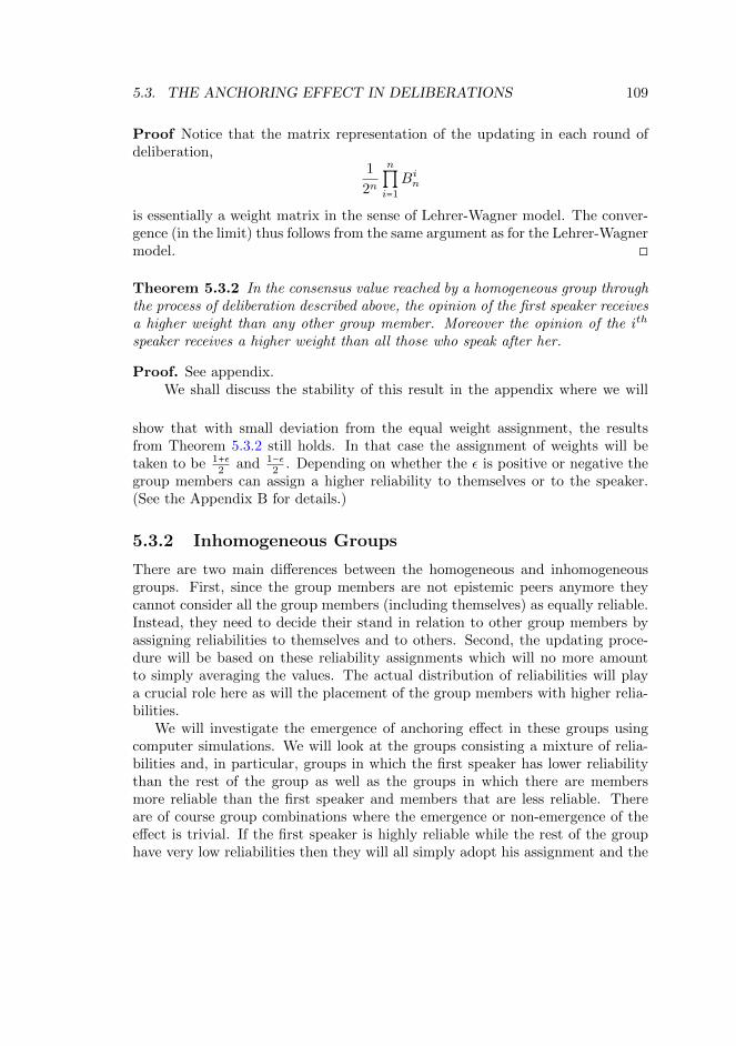
5.3. THE ANCHORING EFFECT IN DELIBERATIONS 109
Proof Notice that the matrix representation of the updating in each round ofdeliberation,
1
2n
n
∏i=1
Bin
is essentially a weight matrix in the sense of Lehrer-Wagner model. The conver-gence (in the limit) thus follows from the same argument as for the Lehrer-Wagnermodel. ◻
Theorem 5.3.2 In the consensus value reached by a homogeneous group throughthe process of deliberation described above, the opinion of the first speaker receivesa higher weight than any other group member. Moreover the opinion of the ith
speaker receives a higher weight than all those who speak after her.
Proof. See appendix.We shall discuss the stability of this result in the appendix where we will
show that with small deviation from the equal weight assignment, the resultsfrom Theorem 5.3.2 still holds. In that case the assignment of weights will betaken to be 1+ε
2and 1−ε
2. Depending on whether the ε is positive or negative the
group members can assign a higher reliability to themselves or to the speaker.(See the Appendix B for details.)
5.3.2 Inhomogeneous Groups
There are two main differences between the homogeneous and inhomogeneousgroups. First, since the group members are not epistemic peers anymore theycannot consider all the group members (including themselves) as equally reliable.Instead, they need to decide their stand in relation to other group members byassigning reliabilities to themselves and to others. Second, the updating proce-dure will be based on these reliability assignments which will no more amountto simply averaging the values. The actual distribution of reliabilities will playa crucial role here as will the placement of the group members with higher relia-bilities.
We will investigate the emergence of anchoring effect in these groups usingcomputer simulations. We will look at the groups consisting a mixture of relia-bilities and, in particular, groups in which the first speaker has lower reliabilitythan the rest of the group as well as the groups in which there are membersmore reliable than the first speaker and members that are less reliable. Thereare of course group combinations where the emergence or non-emergence of theeffect is trivial. If the first speaker is highly reliable while the rest of the grouphave very low reliabilities then they will all simply adopt his assignment and the
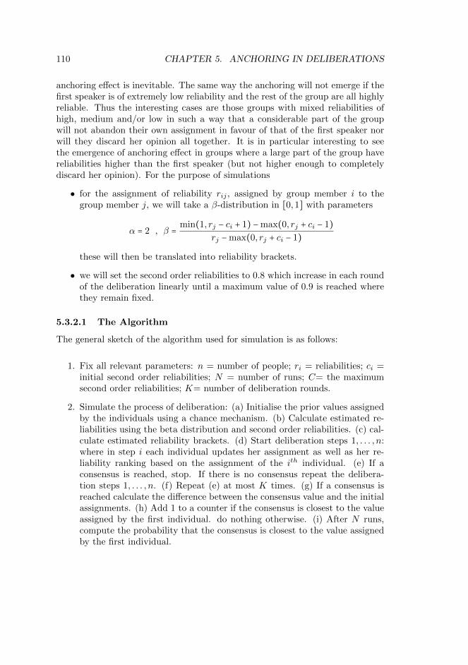
110 CHAPTER 5. ANCHORING IN DELIBERATIONS
anchoring effect is inevitable. The same way the anchoring will not emerge if thefirst speaker is of extremely low reliability and the rest of the group are all highlyreliable. Thus the interesting cases are those groups with mixed reliabilities ofhigh, medium and/or low in such a way that a considerable part of the groupwill not abandon their own assignment in favour of that of the first speaker norwill they discard her opinion all together. It is in particular interesting to seethe emergence of anchoring effect in groups where a large part of the group havereliabilities higher than the first speaker (but not higher enough to completelydiscard her opinion). For the purpose of simulations
• for the assignment of reliability rij , assigned by group member i to thegroup member j, we will take a β-distribution in [0,1] with parameters
α = 2 , β =min(1, rj − ci + 1) −max(0, rj + ci − 1)
rj −max(0, rj + ci − 1)
these will then be translated into reliability brackets.
• we will set the second order reliabilities to 0.8 which increase in each roundof the deliberation linearly until a maximum value of 0.9 is reached wherethey remain fixed.
5.3.2.1 The Algorithm
The general sketch of the algorithm used for simulation is as follows:
1. Fix all relevant parameters: n = number of people; ri = reliabilities; ci =initial second order reliabilities; N = number of runs; C= the maximumsecond order reliabilities; K= number of deliberation rounds.
2. Simulate the process of deliberation: (a) Initialise the prior values assignedby the individuals using a chance mechanism. (b) Calculate estimated re-liabilities using the beta distribution and second order reliabilities. (c) cal-culate estimated reliability brackets. (d) Start deliberation steps 1, . . . , n:where in step i each individual updates her assignment as well as her re-liability ranking based on the assignment of the ith individual. (e) If aconsensus is reached, stop. If there is no consensus repeat the delibera-tion steps 1, . . . , n. (f) Repeat (e) at most K times. (g) If a consensus isreached calculate the difference between the consensus value and the initialassignments. (h) Add 1 to a counter if the consensus is closest to the valueassigned by the first individual. do nothing otherwise. (i) After N runs,compute the probability that the consensus is closest to the value assignedby the first individual.
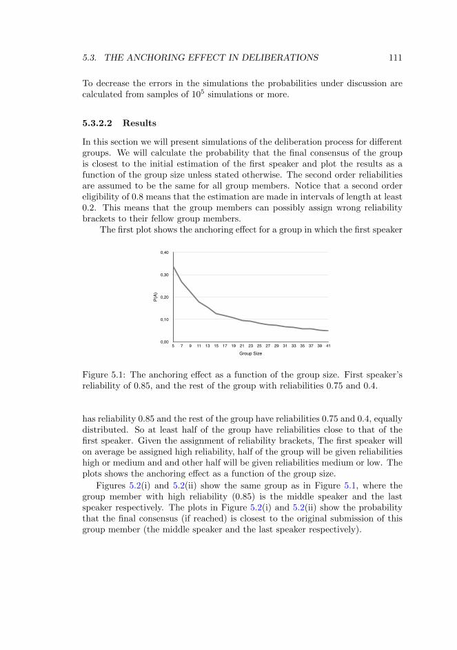
5.3. THE ANCHORING EFFECT IN DELIBERATIONS 111
To decrease the errors in the simulations the probabilities under discussion arecalculated from samples of 105 simulations or more.
5.3.2.2 Results
In this section we will present simulations of the deliberation process for differentgroups. We will calculate the probability that the final consensus of the groupis closest to the initial estimation of the first speaker and plot the results as afunction of the group size unless stated otherwise. The second order reliabilitiesare assumed to be the same for all group members. Notice that a second ordereligibility of 0.8 means that the estimation are made in intervals of length at least0.2. This means that the group members can possibly assign wrong reliabilitybrackets to their fellow group members.
The first plot shows the anchoring effect for a group in which the first speaker5 0,336
7 0,269
9 0,220
11 0,178
13 0,155
15 0,126
17 0,116
19 0,107
21 0,095
23 0,093
25 0,082
27 0,077
29 0,072
31 0,068
33 0,064
35 0,059
37 0,059
39 0,052
41 0,050
43 0,052
45 0,048
47 0,046
49 0,044
51 0,041
53 0,042
55 0,037
57 0,038
P(A)
0,00
0,10
0,20
0,30
0,40
Group Size5 7 9 11 13 15 17 19 21 23 25 27 29 31 33 35 37 39 41
Figure 5.1: The anchoring effect as a function of the group size. First speaker’sreliability of 0.85, and the rest of the group with reliabilities 0.75 and 0.4.
has reliability 0.85 and the rest of the group have reliabilities 0.75 and 0.4, equallydistributed. So at least half of the group have reliabilities close to that of thefirst speaker. Given the assignment of reliability brackets, The first speaker willon average be assigned high reliability, half of the group will be given reliabilitieshigh or medium and and other half will be given reliabilities medium or low. Theplots shows the anchoring effect as a function of the group size.
Figures 5.2(i) and 5.2(ii) show the same group as in Figure 5.1, where thegroup member with high reliability (0.85) is the middle speaker and the lastspeaker respectively. The plots in Figure 5.2(i) and 5.2(ii) show the probabilitythat the final consensus (if reached) is closest to the original submission of thisgroup member (the middle speaker and the last speaker respectively).
112 CHAPTER 5. ANCHORING IN DELIBERATIONS5 0,212 0,1377 0,129 0,1159 0,113 0,099
11 0,083 0,08313 0,074 0,06815 0,064 0,06017 0,056 0,05519 0,049 0,04821 0,045 0,04423 0,042 0,04125 0,038 0,03927 0,035 0,03529 0,034 0,03331 0,031 0,03133 0,029 0,02835 0,028 0,02737 0,026 0,02639 0,026 0,02541 0,024 0,02443 0,022 0,023
45 0,021 0,021
47 0,020 0,020
49 0,020 0,020
51 0,019 0,019
53 0,018 0,018
55 0,018 0,018
57 0,018 0,017
P(A)
0,00
0,06
0,13
0,19
0,25
Group Size5 9 13 17 21 25 29 33 37 41 45 49 53 57
Figure 5.2: The anchoring effect for the middle and last speakers as a functionof the group size. i) Dashed line for the middle speaker with reliability 0.85 andthe rest 0.75 and 0.4. ii) Continuous line for last speaker with reliability 0. 0.85and the rest 0.75 and 0.4.
Comparing Figure 5.1 with Figures 5.2(i) and 5.2(ii), shows how the anchoringeffect depends on the speakers position in the group. In particular, the compar-ison of the plots suggests that anchoring effect depends more on the speaker’sposition in the group compared to her reliability as the same member placed inthe middle or as the last speaker will impose a much smaller anchoring effect. Tosee this more clearly one can compare the anchoring effect for the first speakerin Figure 5.1 with that of the middle and the last speaker in Figures 5.3(i) and5.3(ii) respectively, where the middle and the last speakers have significantlyhigher reliabilities than the rest of the group.
5 0,248 0,1877 0,216 0,1259 0,144 0,099
11 0,090 0,08113 0,074 0,07015 0,079 0,06017 0,061 0,05319 0,056 0,04921 0,049 0,04523 0,042 0,04125 0,040 0,03727 0,036 0,03629 0,033 0,03331 0,031 0,03033 0,030 0,03035 0,028 0,02737 0,026 0,02539 0,025 0,02541 0,024 0,02443 0,021 0,0224545 0,022 0,0215747 0,020 0,0203849 0,020 0,0199551 0,020 0,019153 0,018 0,0190955 0,017 0,0176857 0,017 0,01687
P(A)
0,00
0,08
0,15
0,23
0,30
Group Size5 9 13 17 21 25 29 33 37 41 45 49 53 57
Figure 5.3: The anchoring effect for the middle and the last speakers as a functionof the group size. i) Dashed line for middle speaker with reliability 0.85 and therest 0.55 and 0.4. ii) Continuous line for last speaker with reliability 0.85 and therest 0.55 and 0.4.
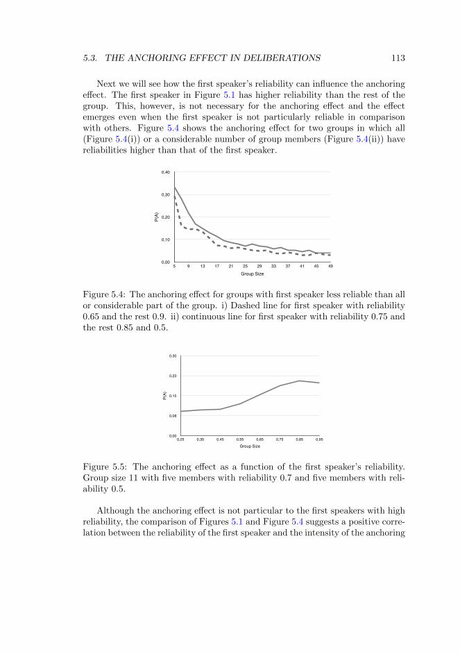
5.3. THE ANCHORING EFFECT IN DELIBERATIONS 113
Next we will see how the first speaker’s reliability can influence the anchoringeffect. The first speaker in Figure 5.1 has higher reliability than the rest of thegroup. This, however, is not necessary for the anchoring effect and the effectemerges even when the first speaker is not particularly reliable in comparisonwith others. Figure 5.4 shows the anchoring effect for two groups in which all(Figure 5.4(i)) or a considerable number of group members (Figure 5.4(ii)) havereliabilities higher than that of the first speaker.
5 0,29418 0,315 0,351 0,3337 0,15934 0,301 0,262 0,2819 0,14352 0,244 0,192 0,218
11 0,147 0,167 0,172 0,16913 0,131 0,152 0,145 0,14915 0,104 0,128 0,128 0,12817 0,073 0,120 0,109 0,11419 0,072 0,105 0,087 0,09621 0,062 0,108 0,065 0,08623 0,066 0,073 0,084 0,07925 0,058 0,086 0,057 0,07127 0,054 0,081 0,077 0,07929 0,048 0,076 0,065 0,07131 0,051 0,074 0,064 0,06933 0,040 0,060 0,058 0,05935 0,038 0,065 0,063 0,06437 0,043 0,065 0,042 0,05339 0,037 0,050 0,054 0,05241 0,032 0,055 0,037 0,04643 0,030 0,05185 0,04985 0,05145 0,040 0,04706 0,03356 0,04047 0,033 0,04688 0,03431 0,04149 0,032 0,04261 0,03829 0,040
P(A)
0,00
0,10
0,20
0,30
0,40
Group Size5 9 13 17 21 25 29 33 37 41 45 49
Figure 5.4: The anchoring effect for groups with first speaker less reliable than allor considerable part of the group. i) Dashed line for first speaker with reliability0.65 and the rest 0.9. ii) continuous line for first speaker with reliability 0.75 andthe rest 0.85 and 0.5.
0,25 0,0910,35 0,0960,45 0,10,55 0,1200,65 0,1540,75 0,1870,85 0,2070,95 0,198 P(
A)
0,00
0,08
0,15
0,23
0,30
Group Size0,25 0,35 0,45 0,55 0,65 0,75 0,85 0,95
Figure 5.5: The anchoring effect as a function of the first speaker’s reliability.Group size 11 with five members with reliability 0.7 and five members with reli-ability 0.5.
Although the anchoring effect is not particular to the first speakers with highreliability, the comparison of Figures 5.1 and Figure 5.4 suggests a positive corre-lation between the reliability of the first speaker and the intensity of the anchoring
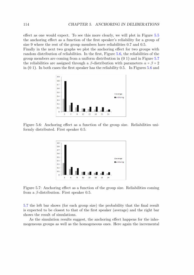
114 CHAPTER 5. ANCHORING IN DELIBERATIONS
effect as one would expect. To see this more clearly, we will plot in Figure 5.5the anchoring effect as a function of the first speaker’s reliability for a group ofsize 9 where the rest of the group members have reliabilities 0.7 and 0.5.Finally in the next two graphs we plot the anchoring effect for two groups withrandom distribution of reliabilities. In the first, Figure 5.6, the reliabilities of thegroup members are coming from a uniform distribution in (0 1) and in Figure 5.7the reliabilities are assigned through a β-distribution with parameters α = β = 2in (0 1). In both cases the first speaker has the reliability 0.5. In Figures 5.6 and
Figure 5.6: Anchoring effect as a function of the group size. Reliabilities uni-formly distributed. First speaker 0.5.
Figure 5.7: Anchoring effect as a function of the group size. Reliabilities comingfrom a β-distribution. First speaker 0.5.
5.7 the left bar shows (for each group size) the probability that the final resultis expected to be closest to that of the first speaker (average) and the right barshows the result of simulations.
As the simulation results suggest, the anchoring effect happens for the inho-mogeneous groups as well as the homogeneous ones. Here again the incremental
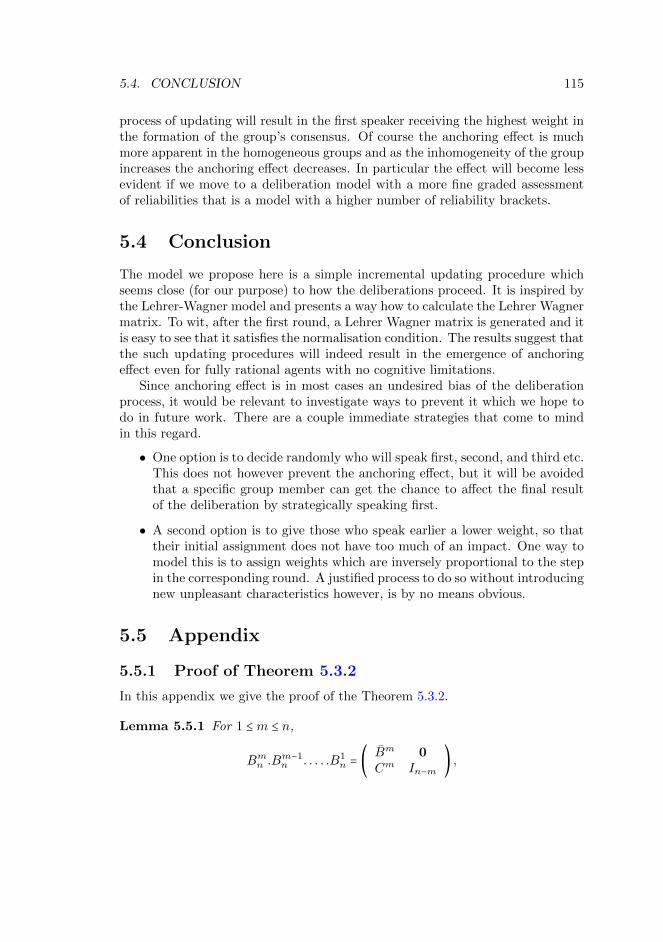
5.4. CONCLUSION 115
process of updating will result in the first speaker receiving the highest weight inthe formation of the group’s consensus. Of course the anchoring effect is muchmore apparent in the homogeneous groups and as the inhomogeneity of the groupincreases the anchoring effect decreases. In particular the effect will become lessevident if we move to a deliberation model with a more fine graded assessmentof reliabilities that is a model with a higher number of reliability brackets.
5.4 Conclusion
The model we propose here is a simple incremental updating procedure whichseems close (for our purpose) to how the deliberations proceed. It is inspired bythe Lehrer-Wagner model and presents a way how to calculate the Lehrer Wagnermatrix. To wit, after the first round, a Lehrer Wagner matrix is generated and itis easy to see that it satisfies the normalisation condition. The results suggest thatthe such updating procedures will indeed result in the emergence of anchoringeffect even for fully rational agents with no cognitive limitations.
Since anchoring effect is in most cases an undesired bias of the deliberationprocess, it would be relevant to investigate ways to prevent it which we hope todo in future work. There are a couple immediate strategies that come to mindin this regard.
• One option is to decide randomly who will speak first, second, and third etc.This does not however prevent the anchoring effect, but it will be avoidedthat a specific group member can get the chance to affect the final resultof the deliberation by strategically speaking first.
• A second option is to give those who speak earlier a lower weight, so thattheir initial assignment does not have too much of an impact. One way tomodel this is to assign weights which are inversely proportional to the stepin the corresponding round. A justified process to do so without introducingnew unpleasant characteristics however, is by no means obvious.
5.5 Appendix
5.5.1 Proof of Theorem 5.3.2
In this appendix we give the proof of the Theorem 5.3.2.
Lemma 5.5.1 For 1 ≤m ≤ n,
Bmn .Bm−1n . . . . .B1
n = (Bm 0Cm In−m
) ,

116 CHAPTER 5. ANCHORING IN DELIBERATIONS
where
Bm =
⎛⎜⎜⎜⎜⎜⎜⎜⎜⎜⎜⎝
2m−1 + 1 2m−2 ... 20
2m−1 2m−2 + 1 ... 20
2m−1 2m−2 ... 20
. . . .
. . . .
. . . .2m−1 2m−2 ... 20 + 1
⎞⎟⎟⎟⎟⎟⎟⎟⎟⎟⎟⎠m×m
0 is an m× (n−m) zero matrix, In−m is the unite (n−m)× (n−m) matrix and
Cm =
⎛⎜⎜⎜⎜⎜⎜⎜⎜⎝
2m−1 2m−2 ... 20
2m−1 2m−2 ... 20
. . . .
. . . .
. . . .2m−1 2m−2 ... 20
⎞⎟⎟⎟⎟⎟⎟⎟⎟⎠(n−m)×m
Proof For m = 1 the result is trivially true. Suppose it is true for m and we shallshow that it holds for m + 1.
Bm+1n .Bm−1
n . . . . .B1n = B
m+1n .(
Bm 0Cm In−m
)
= (Am+1n + In).(
Bm 0Cm In−m
)
= Am+1n .(
Bm 0Cm In−m
) + In.(Bm 0Cm In−m
) =
⎛⎜⎜⎜⎜⎜⎜⎜⎜⎜⎜⎜⎜⎜⎜⎜⎜⎜⎝
2m−1 2m−2 ... 20 1 0 ... 02m−1 2m−2 ... 20 1 0 ... 0. . . . . . . .. . . . . . . .. . . . . . . .
2m−1 2m−2 ... 20 1 0 ... 02m−1 2m−2 ... 20 1 0 ... 0. . . . . . . .. . . . . . . .
2m−1 2m−2 ... 20 1 0 ... 0
⎞⎟⎟⎟⎟⎟⎟⎟⎟⎟⎟⎟⎟⎟⎟⎟⎟⎟⎠
+
⎛⎜⎜⎜⎜⎜⎜⎜⎜⎜⎜⎜⎜⎜⎜⎜⎜⎜⎝
2m−1 + 1 2m−2 ... 20 0 ... 02m−1 2m−2 + 1 ... 20 0 ... 0. . . . . . .. . . . . . .. . . . . . .
2m−1 2m−2 ... 20 + 1 0 ... 02m−1 2m−2 ... 20 1 ... 0. . . . . ... .. . . . . ... .
2m−1 2m−2 ... 20 0 ... 1
⎞⎟⎟⎟⎟⎟⎟⎟⎟⎟⎟⎟⎟⎟⎟⎟⎟⎟⎠
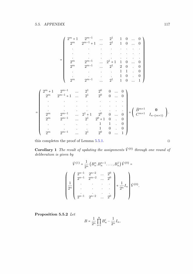
5.5. APPENDIX 117
=
⎛⎜⎜⎜⎜⎜⎜⎜⎜⎜⎜⎜⎜⎜⎜⎜⎜⎜⎝
2m + 1 2m−1 ... 21 1 0 ... 02m 2m−1 + 1 ... 21 1 0 ... 0. . . . . . . .. . . . . . . .. . . . . . . .
2m 2m−1 ... 21 + 1 1 0 ... 02m 2m−1 ... 21 2 0 . 0. . . . 1 1 . 0. . . . 1 0 . 0
2m 2m−1 ... 21 1 0 ... 1
⎞⎟⎟⎟⎟⎟⎟⎟⎟⎟⎟⎟⎟⎟⎟⎟⎟⎟⎠
=
⎛⎜⎜⎜⎜⎜⎜⎜⎜⎜⎜⎜⎜⎜⎜⎜⎜⎜⎝
2m + 1 2m−1 ... 21 20 0 ... 02m 2m−1 + 1 ... 21 20 0 ... 0. . . . . . . .. . . . . . . .. . . . . . . .
2m 2m−1 ... 21 + 1 20 0 ... 02m 2m−1 ... 21 20 + 1 0 . 0. . . . 1 1 . 0. . . . 1 0 . 0
2m 2m−1 ... 21 20 0 ... 1
⎞⎟⎟⎟⎟⎟⎟⎟⎟⎟⎟⎟⎟⎟⎟⎟⎟⎟⎠
= (Bm+1 0Cm+1 In−(m+1)
) .
this completes the proof of Lemma 5.5.1. ◻
Corollary 1 The result of updating the assignments V (0) through one round ofdeliberation is given by
V (1) =1
2n(Bnn .B
n−1n . . . . ,B1
n) V(0) =
⎛⎜⎜⎜⎜⎜⎜⎜⎜⎝
1
2n
⎛⎜⎜⎜⎜⎜⎜⎜⎜⎝
2n−1 2n−2 ... 20
2n−1 2m−2 ... 20
. . . .
. . . .
. . . .2n−1 2n−2 ... 20
⎞⎟⎟⎟⎟⎟⎟⎟⎟⎠
+1
2nIn
⎞⎟⎟⎟⎟⎟⎟⎟⎟⎠
V (0).
Proposition 5.5.2 Let
B =1
2n
n
∏i=1
Bin −1
2nIn,
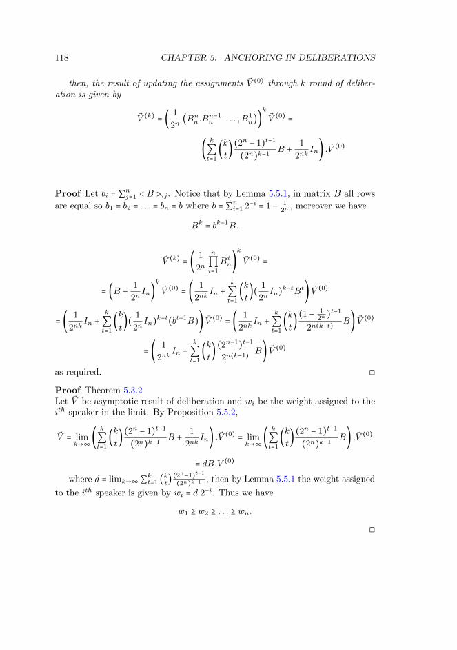
118 CHAPTER 5. ANCHORING IN DELIBERATIONS
then, the result of updating the assignments V (0) through k round of deliber-ation is given by
V (k) = (1
2n(Bnn .B
n−1n . . . . ,B1
n))k
V (0) =
(k
∑t=1
(k
t)(2n − 1)t−1
(2n)k−1B +
1
2nkIn) .V
(0)
Proof Let bi = ∑nj=1 < B >ij . Notice that by Lemma 5.5.1, in matrix B all rows
are equal so b1 = b2 = . . . = bn = b where b = ∑ni=1 2−i = 1 − 1
2n, moreover we have
Bk = bk−1B.
V (k) = (1
2n
n
∏i=1
Bin)
k
V (0) =
= (B +1
2nIn)
k
V (0) = (1
2nkIn +
k
∑t=1
(k
t)(
1
2nIn)
k−tBt) V (0)
= (1
2nkIn +
k
∑t=1
(k
t)(
1
2nIn)
k−t(bt−1B)) V (0) = (1
2nkIn +
k
∑t=1
(k
t)(1 − 1
2n)t−1
2n(k−t)B) V (0)
= (1
2nkIn +
k
∑t=1
(k
t)(2n−1)t−1
2n(k−1) B) V (0)
as required. ◻
Proof Theorem 5.3.2Let V be asymptotic result of deliberation and wi be the weight assigned to theith speaker in the limit. By Proposition 5.5.2,
V = limk→∞
(k
∑t=1
(k
t)(2n − 1)t−1
(2n)k−1B +
1
2nkIn) .V
(0) = limk→∞
(k
∑t=1
(k
t)(2n − 1)t−1
(2n)k−1B) .V (0)
= dB.V (0)
where d = limk→∞∑kt=1 (k
t) (2
n−1)t−1(2n)k−1 , then by Lemma 5.5.1 the weight assigned
to the ith speaker is given by wi = d.2−i. Thus we have
w1 ≥ w2 ≥ . . . ≥ wn.
◻

5.5. APPENDIX 119
5.5.2 Stability Result
Next we will investigate the stability of our results for the homogeneous groups byshowing that the results still hold for small changes in the equal weight assump-tion. Here the group members consider small deviation from the equal weightsby assigning 1−ε
2to the speaker and 1+ε
2to themselves. As before, after the ith
group member speaks, everyone will update their assignment as a weighted aver-age of their current value and that announced by the ith speaker while assigninga slightly higher/lower weight to themselves as opposed to the speaker. Thisprocess can again be represented by matrix multiplication as before by replacingthe matrices Bin with
Bi′n = Bin − εEin
whereEjn = B
jn − 2Ajn.
Thus for example, in group of size 3, the matrix
B23 =
⎛⎜⎝
1 1 00 2 00 1 1
⎞⎟⎠
will be replaced by
B2′3 =
⎛⎜⎝
1 1 00 2 00 1 1
⎞⎟⎠+ ε
⎛⎜⎝
⎛⎜⎝
1 1 00 2 00 1 1
⎞⎟⎠− 2
⎛⎜⎝
0 1 00 1 00 1 0
⎞⎟⎠
⎞⎟⎠
=⎛⎜⎝
1 1 00 2 00 1 1
⎞⎟⎠+ ε
⎛⎜⎝
1 −1 00 0 00 −1 1
⎞⎟⎠
=⎛⎜⎝
1 + ε 1 − ε 00 2 00 1 − ε 1 + ε
⎞⎟⎠.
In this new setting we shall again have that the result of one round of delib-eration is given as
V (1) =1
2n
n
∏i=1
Bi′n .V(0)
and after k round of deliberation we shall have
V (k) = (1
2n
n
∏i=1
Bi′n)
k
V (0).
We shall first prove the corresponding versions of Lemma 5.5.1 for this setting.
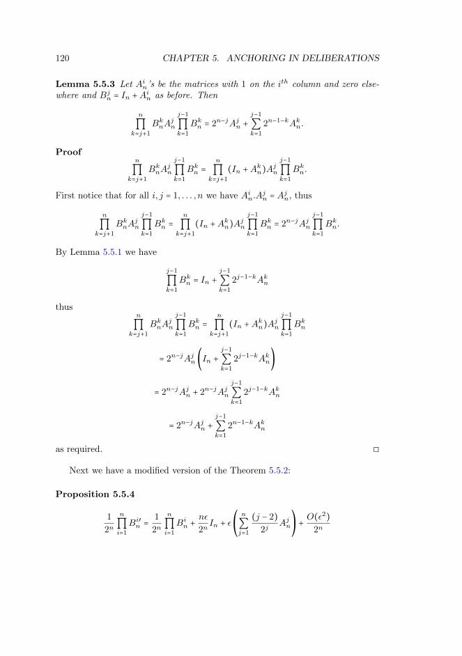
120 CHAPTER 5. ANCHORING IN DELIBERATIONS
Lemma 5.5.3 Let Ain’s be the matrices with 1 on the ith column and zero else-where and Bjn = In +A
in as before. Then
n
∏k=j+1
BknAjn
j−1
∏k=1
Bkn = 2n−jAjn +j−1
∑k=1
2n−1−kAkn.
Proofn
∏k=j+1
BknAjn
j−1
∏k=1
Bkn =n
∏k=j+1
(In +Akn)A
jn
j−1
∏k=1
Bkn.
First notice that for all i, j = 1, . . . , n we have Ain.Ajn = A
jn, thus
n
∏k=j+1
BknAjn
j−1
∏k=1
Bkn =n
∏k=j+1
(In +Akn)A
jn
j−1
∏k=1
Bkn = 2n−jAjn
j−1
∏k=1
Bkn.
By Lemma 5.5.1 we have
j−1
∏k=1
Bkn = In +j−1
∑k=1
2j−1−kAkn
thusn
∏k=j+1
BknAjn
j−1
∏k=1
Bkn =n
∏k=j+1
(In +Akn)A
jn
j−1
∏k=1
Bkn
= 2n−jAjn (In +j−1
∑k=1
2j−1−kAkn)
= 2n−jAjn + 2n−jAjn
j−1
∑k=1
2j−1−kAkn
= 2n−jAjn +j−1
∑k=1
2n−1−kAkn
as required. ◻
Next we have a modified version of the Theorem 5.5.2:
Proposition 5.5.4
1
2n
n
∏i=1
Bi′n =1
2n
n
∏i=1
Bin +nε
2nIn + ε
⎛
⎝
n
∑j=1
(j − 2)
2jAjn
⎞
⎠+O(ε2)
2n
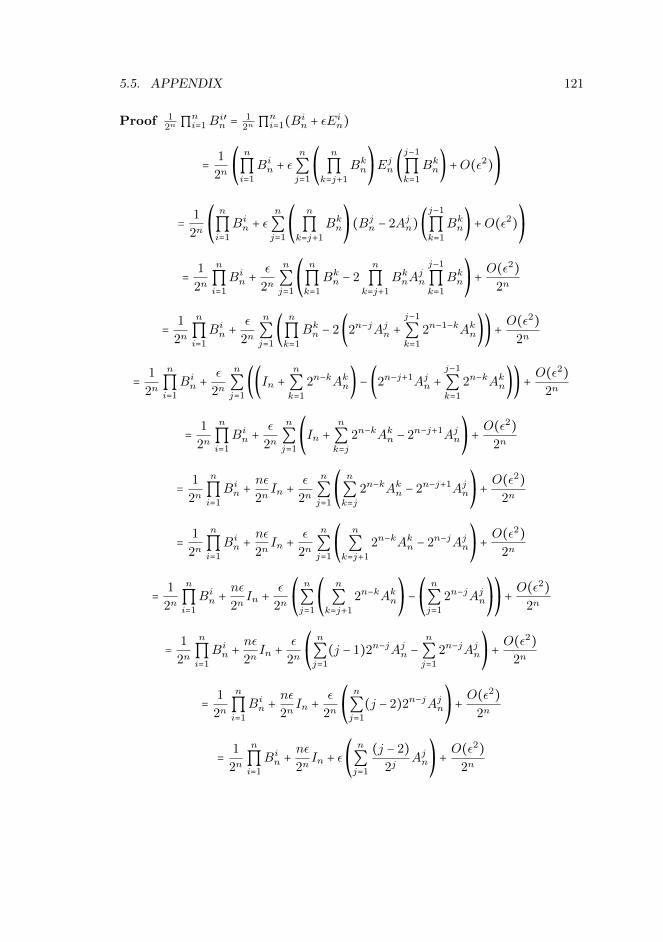
5.5. APPENDIX 121
Proof 12n ∏
ni=1B
i′n = 1
2n ∏ni=1(B
in + εE
in)
=1
2n⎛
⎝
n
∏i=1
Bin + εn
∑j=1
⎛
⎝
n
∏k=j+1
Bkn⎞
⎠Ejn (
j−1
∏k=1
Bkn) +O(ε2)⎞
⎠
=1
2n⎛
⎝
n
∏i=1
Bin + εn
∑j=1
⎛
⎝
n
∏k=j+1
Bkn⎞
⎠(Bjn − 2Ajn)(
j−1
∏k=1
Bkn) +O(ε2)⎞
⎠
=1
2n
n
∏i=1
Bin +ε
2n
n
∑j=1
⎛
⎝
n
∏k=1
Bkn − 2n
∏k=j+1
BknAjn
j−1
∏k=1
Bkn⎞
⎠+O(ε2)
2n
=1
2n
n
∏i=1
Bin +ε
2n
n
∑j=1
(n
∏k=1
Bkn − 2(2n−jAjn +j−1
∑k=1
2n−1−kAkn)) +O(ε2)
2n
=1
2n
n
∏i=1
Bin +ε
2n
n
∑j=1
((In +n
∑k=1
2n−kAkn) − (2n−j+1Ajn +j−1
∑k=1
2n−kAkn)) +O(ε2)
2n
=1
2n
n
∏i=1
Bin +ε
2n
n
∑j=1
⎛
⎝In +
n
∑k=j
2n−kAkn − 2n−j+1Ajn⎞
⎠+O(ε2)
2n
=1
2n
n
∏i=1
Bin +nε
2nIn +
ε
2n
n
∑j=1
⎛
⎝
n
∑k=j
2n−kAkn − 2n−j+1Ajn⎞
⎠+O(ε2)
2n
=1
2n
n
∏i=1
Bin +nε
2nIn +
ε
2n
n
∑j=1
⎛
⎝
n
∑k=j+1
2n−kAkn − 2n−jAjn⎞
⎠+O(ε2)
2n
=1
2n
n
∏i=1
Bin +nε
2nIn +
ε
2n⎛
⎝
n
∑j=1
⎛
⎝
n
∑k=j+1
2n−kAkn⎞
⎠−⎛
⎝
n
∑j=1
2n−jAjn⎞
⎠
⎞
⎠+O(ε2)
2n
=1
2n
n
∏i=1
Bin +nε
2nIn +
ε
2n⎛
⎝
n
∑j=1
(j − 1)2n−jAjn −n
∑j=1
2n−jAjn⎞
⎠+O(ε2)
2n
=1
2n
n
∏i=1
Bin +nε
2nIn +
ε
2n⎛
⎝
n
∑j=1
(j − 2)2n−jAjn⎞
⎠+O(ε2)
2n
=1
2n
n
∏i=1
Bin +nε
2nIn + ε
⎛
⎝
n
∑j=1
(j − 2)
2jAjn
⎞
⎠+O(ε2)
2n
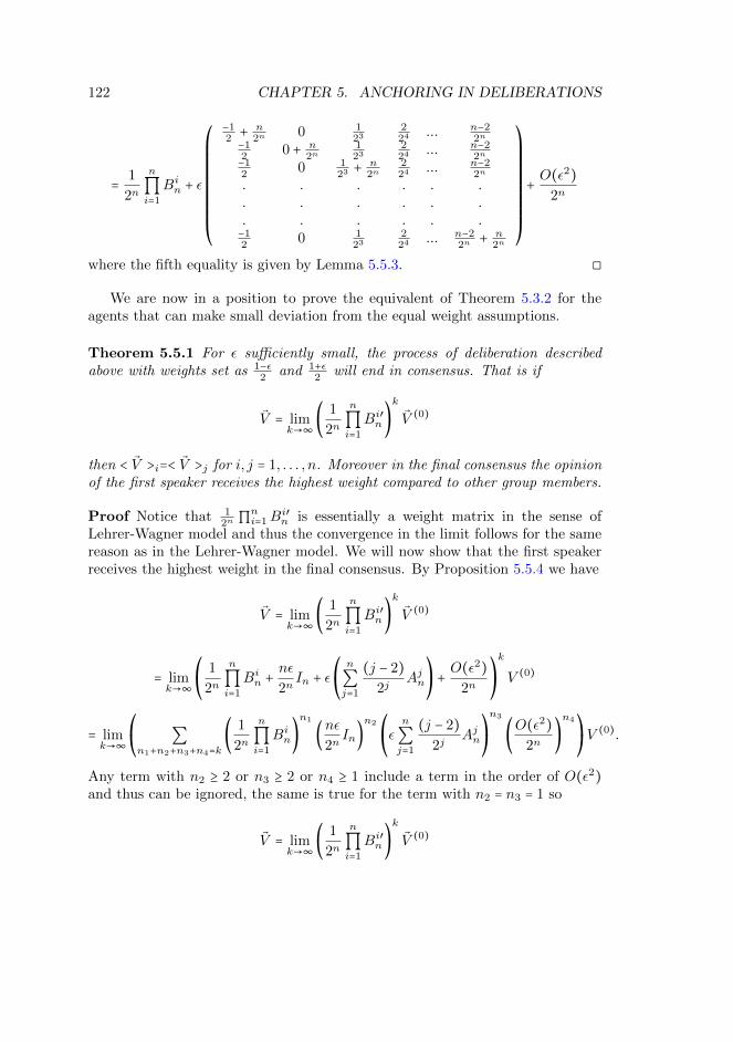
122 CHAPTER 5. ANCHORING IN DELIBERATIONS
=1
2n
n
∏i=1
Bin + ε
⎛⎜⎜⎜⎜⎜⎜⎜⎜⎜⎜⎝
−12+ n
2n0 1
23224 ... n−2
2n−12
0 + n2n
123
224 ... n−2
2n−12
0 123 +
n2n
224 ... n−2
2n
. . . . . .
. . . . . .
. . . . . .−12
0 123
224 ... n−2
2n+ n
2n
⎞⎟⎟⎟⎟⎟⎟⎟⎟⎟⎟⎠
+O(ε2)
2n
where the fifth equality is given by Lemma 5.5.3. ◻
We are now in a position to prove the equivalent of Theorem 5.3.2 for theagents that can make small deviation from the equal weight assumptions.
Theorem 5.5.1 For ε sufficiently small, the process of deliberation describedabove with weights set as 1−ε
2and 1+ε
2will end in consensus. That is if
V = limk→∞
(1
2n
n
∏i=1
Bi′n)
k
V (0)
then < V >i=< V >j for i, j = 1, . . . , n. Moreover in the final consensus the opinionof the first speaker receives the highest weight compared to other group members.
Proof Notice that 12n ∏
ni=1B
i′n is essentially a weight matrix in the sense of
Lehrer-Wagner model and thus the convergence in the limit follows for the samereason as in the Lehrer-Wagner model. We will now show that the first speakerreceives the highest weight in the final consensus. By Proposition 5.5.4 we have
V = limk→∞
(1
2n
n
∏i=1
Bi′n)
k
V (0)
= limk→∞
⎛
⎝
1
2n
n
∏i=1
Bin +nε
2nIn + ε
⎛
⎝
n
∑j=1
(j − 2)
2jAjn
⎞
⎠+O(ε2)
2n⎞
⎠
k
V (0)
= limk→∞
⎛
⎝∑
n1+n2+n3+n4=k(
1
2n
n
∏i=1
Bin)
n1
(nε
2nIn)
n2 ⎛
⎝εn
∑j=1
(j − 2)
2jAjn
⎞
⎠
n3
(O(ε2)
2n)
n4⎞
⎠V (0).
Any term with n2 ≥ 2 or n3 ≥ 2 or n4 ≥ 1 include a term in the order of O(ε2)and thus can be ignored, the same is true for the term with n2 = n3 = 1 so
V = limk→∞
(1
2n
n
∏i=1
Bi′n)
k
V (0)
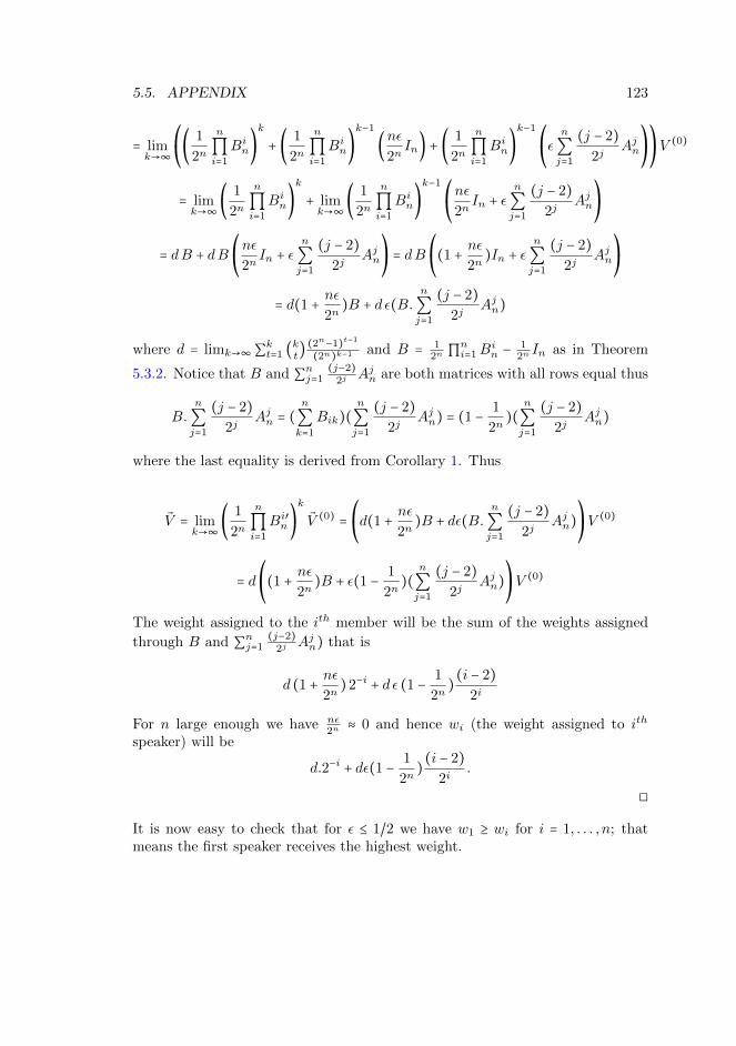
5.5. APPENDIX 123
= limk→∞
⎛
⎝(
1
2n
n
∏i=1
Bin)
k
+ (1
2n
n
∏i=1
Bin)
k−1
(nε
2nIn) + (
1
2n
n
∏i=1
Bin)
k−1⎛
⎝εn
∑j=1
(j − 2)
2jAjn
⎞
⎠
⎞
⎠V (0)
= limk→∞
(1
2n
n
∏i=1
Bin)
k
+ limk→∞
(1
2n
n
∏i=1
Bin)
k−1⎛
⎝
nε
2nIn + ε
n
∑j=1
(j − 2)
2jAjn
⎞
⎠
= dB + dB⎛
⎝
nε
2nIn + ε
n
∑j=1
(j − 2)
2jAjn
⎞
⎠= dB
⎛
⎝(1 +
nε
2n)In + ε
n
∑j=1
(j − 2)
2jAjn
⎞
⎠
= d(1 +nε
2n)B + d ε(B.
n
∑j=1
(j − 2)
2jAjn)
where d = limk→∞∑kt=1 (k
t) (2
n−1)t−1(2n)k−1 and B = 1
2n ∏ni=1B
in −
12nIn as in Theorem
5.3.2. Notice that B and ∑nj=1
(j−2)2j
Ajn are both matrices with all rows equal thus
B.n
∑j=1
(j − 2)
2jAjn = (
n
∑k=1
Bik)(n
∑j=1
(j − 2)
2jAjn) = (1 −
1
2n)(
n
∑j=1
(j − 2)
2jAjn)
where the last equality is derived from Corollary 1. Thus
V = limk→∞
(1
2n
n
∏i=1
Bi′n)
k
V (0) =⎛
⎝d(1 +
nε
2n)B + dε(B.
n
∑j=1
(j − 2)
2jAjn)
⎞
⎠V (0)
= d⎛
⎝(1 +
nε
2n)B + ε(1 −
1
2n)(
n
∑j=1
(j − 2)
2jAjn)
⎞
⎠V (0)
The weight assigned to the ith member will be the sum of the weights assigned
through B and ∑nj=1
(j−2)2j
Ajn) that is
d (1 +nε
2n)2−i + d ε (1 −
1
2n)(i − 2)
2i
For n large enough we have nε2n
≈ 0 and hence wi (the weight assigned to ith
speaker) will be
d.2−i + dε(1 −1
2n)(i − 2)
2i.
◻
It is now easy to check that for ε ≤ 1/2 we have w1 ≥ wi for i = 1, . . . , n; thatmeans the first speaker receives the highest weight.

124 CHAPTER 5. ANCHORING IN DELIBERATIONS
Chapter 6
Conclusion
In this thesis, we studied four problems of long standing interest in philosophyusing mathematical and computational methods. The problems we investigatedhere belong to different philosophical discipline and each has attracted attentionfrom different parts of philosophical community. The treatment of inconsistencieshas been of interest to both philosophers and mathematicians. Logic of condi-tionals has been a main stream topic in philosophy for at least several decadesand the study of rational deliberation and related issues has been of interests toepistemologists, political philosophers and philosophers of social sciences.
Our goal was to demonstrate that a wide range of problems in philosophy canbe fruitfully studied in the approach that has come to be known as the scientificphilosophy. That is by means of scientific methodology such as application ofmathematical modelling and computational methods. The goal was to showthe advantages of such methodology in addressing, or at least further clarifying,many issues and concerns with respect to the philosophical investigation of thesetopics. From these, we hope that the advantages of the scientific approach tophilosophical problems of similar nature would be evident.
As already pointed out, our advocacy of the the scientific methods is by nomeans intended to imply that all problems of philosophical nature should or evencan be adequately represented in a formal machinery or investigated by means offormal and computational methods. The aim was to further motivate the benefitsof employing mathematical and computational methods along side the traditionalphilosophical toolbox as they allow for precise and exact argumentations andextensive study of relevant solution spaces.
The studies presented in this thesis, each introduce further work in theirrespective areas and the methodologies employed for the study of these issuespresent immediate generalisations and seem to facilitate the investigation of more
125
126 CHAPTER 6. CONCLUSION
general cases. The formal machinery used for the study of probabilistic conse-quence relation and modelling the learning of indicative conditionals seem toprovide natural extensions to be considered for the more general cases. Themodels developed for rational deliberation and the study of the anchoring effectcan also be considered as base models that can be further developed into morecomplex ones by introducing more relevant factors.
More precisely, the work presented on dealing with inconsistent evidence begsfor further investigation of distance measures and better justified updating mech-anisms. In particular, we hope to study mechanisms for updating the weightsof information when dealing with prioritised evidence. That is, how to updatethe degree of entrenchment of the information in the belief set (along with theirprobabilities).
The work on leaning indicative conditionals should be further developed tobetter understand the effect of introducing causal structures and to investigatethe similar approach for dealing with counter-factual cases. We also hope toinvestigate whether KL distance can be replaced with another distance measurewith better mathematical properties including, for example, symmetry.
The models developed for group deliberation and the study of the anchoringeffect in deliberations are toy models that include many abstractions. We hopeto further develop these models to incorporate a wider range of relevant charac-teristics of the deliberating agents and to allow for private communications bythe agents both amongst themselves as well as with sources outside the group.
Bibliography
[van Aken et al.2004] van Aaken, A., List, C. and Luetge, C. (eds) (2004). De-liberation and Decision: Economics, Constitutional Theory and DeliberativeDemocracy. Ashgate.
[Alchourron et. al.1985] Alchourrn, C. E., Gadenfors, P., and Makinson, D.(1985). ”On the logic of theory change: Partial meet contraction and revisionfunctions”, Journal of Symbolic Logic 50: 510-530.
[3] Angere, S. (2010). Knowledge in a Social Network. Preprint. Department ofPhilosphy. Lund University.
[Arlo-Costa1990] Arlo-Costa, H. (1990). ”Conditionals and Monotonic Belief Re-visions: The Success Postulate?”, Studia Logica, 49(4): 557–566.
[Bohman & Rehg 1997] Bohman, J. and Rehg, W. (eds) (1997). DeliberativeDemocracy. s on Reason and Politics. Cambridge (Mass.): MIT Press.
[Bovens & Hartmann 2003] Bovens, L. and Hartmann, S. (2003). Bayesian Epis-temology. Oxford: Oxford University Press.
[Cohen 1986] Cohen, J. (1986). An Epistemic Conception of Democracy. Ethics97(1): 26–38. The University of Chicago Press.
[Cohen 1989a] Cohen, J. (1989). Deliberation and Democratic Legitimacy. TheGood Polity: Normative Analysis of the State 17–34 Hamlin A and Pettit P.(eds). Oxford: Blackwell.
[Cohen 1989b] Cohen, J. (1989). The Economic Basis of Deliberative Democracy.Social Philosophy and Policy 6(2): 25–50.
[da Costa 1974] da Costa, N.C.A. (1974). On the Theory of Inconsistent FormalSystems, Notre Dame Journal of Formal Logic 15(4): 497-510.
127
128 BIBLIOGRAPHY
[da Costa 1989] da Costa, N.C.A. and Subrahmanian, V.S. (1989). ”Paraconsis-tent logic as a formalism for reasoning about inconsistent knowledge bases”,Artificial Intelligence in Medicine 1: 167-174.
[da Costa 1998] da Costa, N.C.A. (1998), ”Paraconsistent logic”, StanisawJakowski Memorial Symposium 29–35.
[Christiano 1997] Christiano, T. (1997). The Significance of Public Deliberation.Bohman and Rehg (1997): 243–278.
[Christiano 2004] Christiano, T. (2004). The Authority of Democracy. Journalof Political Philosophy 12(3): 266–290.
[Diaconis & Zabell 1982] Diaconis, P. and S. Zabell (1982). Updating SubjectiveProbability, Journal of the American Statistical Association 77: 822–830.
[Dietrich & Spiekermann 2010] Dietrich, F. and Spiekermann, K.(2010). Epistemic democracy with defensible premises. Avail-able at http://www.franzdietrich.net/Papers/DietrichSpiekermann-EpistemicDemocracy.pdf.
[Dietrich 2006] Dietrich, F. (2006). General Representation of Epistemically Op-timal Procedures. Social Choice and Welfare 26(2): 263–283.
[Douven 2012] Douven, I. (2012). Learning Conditional Information, Mind &Language 27 (3): 239–263.
[Douven & Dietz 2011] Douven, I. and R. Dietz (2011). A Puzzle about Stal-naker’s Hypothesis, Topoi 30: 31–37.
[Douven & Romeijn 2012] Douven, I. and J. W. Romeijn (2012). A New Resolu-tion of the Judy Benjamin Problem, Mind 120 (479): 637–670.
[Dryzek 1990] Dryzek, J. (1990). Discursive Democracy. Cambridge: CambridgeUniversity Press.
[Dryzek & Niemeyer 2010] Dryzek, J. and S. Niemeyer (2010). Foundations andFrontiers of Deliberative Governance. Oxford: Oxford University Press.
[Duran & Arnold 2013] Duran, J. M. and Arnold, E. (2013). Computer Simula-tions and the Changing Face of Scientific Experimentation. Cambridge Schol-ars Publishing.
[Elga 2007] Elga, A. (2007). Reflection and Disagreement. Nous 41(3): 478–502.Also in: P. Grim, I. Flora, and A. Plakias (eds.): The Philosopher’s Annual27 (2007).
BIBLIOGRAPHY 129
[Elster 1998] Elster, J. (eds) (1998). Deliberative Democracy Cambridge: Cam-bridge University Press.
[Estlund 1993] Estlund, D. (1993). Whos Afraid of Deliberative Democracy?On the Strategic/Deliberative Dichotomy in Recent Constitutional Jurispru-dence. Texas Law Review 71:1437-1477.
[Estlund 1994] Estlund, D. (1994). Opinion Leaders, Independence, and Con-dorcets Jury Theorem. Theory and Decision 36(2):131–162.
[Estlund 1997] Estlund, D. (1997). Beyond Fairness and Deliberation: The Epis-temic Dimension of Democratic Authority. Bohman and Rehg (1997): 173–204.
[Estlund 2009] Estlund, D. (2009). Democratic Authority: A PhilosophicalFramework. Princeton: Princeton University Press.
[Falkenhainer et. al. 1989] Falkenhainer, B., Forbus, K. D., and Gentner, D.(1989). ”The Structure mapping Engine: Algorithms and Examples.” Ar-tificial Intelligence, 41:1–63.
[Fearon 1998] Fearon, J. D. (1998). Deliberation as Discussion. DeliberativeDemocracy:44–68. Elster (eds) Cambridge: Cambridge University Press.
[Fitelson & Zalta 2007] Fitelson, B. and Zalta, E. N. (2007). ”Steps Toward aComputational Metaphysics”, Journal of Philosophical Logic, 36(2): 227–247.
[van Fraassen 1981] Fraassen, B. van (1981). A Problem for Relative InformationMinimizers in Probability Kinematics, British Journal for the Philosophy ofScience 32: 375–379.
[Goodin 2008] Goodin, R.E. (2008). Innovating Democracy: Democratic TheoryAnd Practice After The Deliberative Turn. Oxford: Oxford University Press.
[Hartmann et. al. 2009] Hartmann, S., C. Martini and J. Sprenger (2009). Con-sensual Decision-Making Among Epistemic Peers. Episteme 6: 110–129.
[Hegselmann & Krause 2002] Hegselmann, R. and U. Krause (2002). OpinionDynamics and Bounded Confidence: Models, Analysis and Simulation. Jour-nal of Artificial Societies and Social Simulation 5(3).
[Hegselmann & Krause 2006] Hegselmann, R. and U. Krause (2006). Truth andCognitive Division of Labour: First Steps Towards a Computer Aided SocialEpistemology. Journal of Artificial Societies and Social Simulation 9(3).
130 BIBLIOGRAPHY
[Hegselmann & Krause 2009] Hegselmann, R. and U. Krause (2009). Delibera-tive Exchange, Truth, and Cognitive Division of Labour: A Low-ResolutionModeling Approach. Episteme 6: 130–144.
[Holyoak & Thagard 1989] Holyoak, K. J., and Thagard, P. (1989). ”AnalogicalMapping by Constraint Satisfaction.” Cognitive Science, 13: 295–355.
[Holyoak & Thagard 1995] Holyoak, K. J., and Thagard, P. (1995). MentalLeaps: Analogy in Creative Thought. Cambridge, MA: MIT Press/BradfordBooks.
[Kahneman et. al. 2006] Kahneman, D., Krueger, A., Schkade, D., Schwarz, N.,and Stone, A. (2006). Would you be Happier if you Were Richer? A FocusingIllusion. Science 312(5782): 1908–10.
[Kern-Isberner 2001] Kern-Isberner, G. (2001). Conditionals in NonmonotonicReasoning and Belief Revision. Berlin: Springer.
[Knight 2002] Knight, K. M. (2002). Doctoral Thesis, University of Manchester,UK. [see http://www.maths.manchester.ac.uk/ jeff]
[Kulkarni & Simon 1988] Kulkarni, D. and Simon, H. (1988). ”The Processes ofScientific Discovery: The Strategy of Experimentation.” Cognitive Science,12:139–175.
[Ladyman & Ross 2009] Ladyman, J., and Ross, D. (2009). Every Thing MustGo: Metaphysics Naturalized. Oxford University Press.
[Langley et. al. 1987 ] Langley, P., Simon, H., Bradshaw, G., and Zytkow, J.(1987). Scientific Discovery. Cambridge, MA: MIT Press/Bradford Books.
[Lehrer 1976] Lehrer, K. (1976). When Rational Disagreement is Impossible.Nous 10: 327–332.
[Lehrer & Wagner 1981] Lehrer, K. and C. Wagner (1981). Rational Consensusin Science and Society. Dordrecht: Reidel.
[Leitgeb 2013] Leitgeb, H., (2013). ”Scientific Philosophy, Mathematical Philos-ophy, and All That”, Metaphilosophy, 44(3): 267–275.
[Lewis 1976] Lewis, D. (1976). Probabilities of Conditionals and ConditionalProbabilities, Philosophical Review 85: 297–315.
[List & Goodin 2001] List, C. and Goodin, R.E. (2001). Epistemic democracy:Generalizing the Condorcet Jury Theorem. Journal of Political Philosophy 9:277–306.
BIBLIOGRAPHY 131
[Maddy 2009] Maddy, P. (2009). Second Philosophy, Oxford University Press.
[Manin 1987] Manin B. (1987). On Legitimacy and Political Deliberation. Polit-ical Theory 15(3): 338–368.
[Marti 2006] Marti, J.L. (2006). The Epistemic Conception of DeliberativeDemocracy Defended. Reasons, Rightness and Equal Political Liberty. De-liberative Democracy and Its Discontents. National and Post-national Chal-lenges. Besson, S. and Marti, J.L. (eds). London: Ashgate.
[Nino 1996] Nino C.S. (1996). The Constitution of Deliberative Democracy. NewHaven: Yale University Press.
[Olsson 2011] Olsson, E.J. (2011). A Bayesian simulation model of group delib-eration and polarization. Bayesian Argumentation. Zenker, F. (ed.). SyntheseLibrary, Springer Verlag.
[57] Olsson, E.J. (2011b). A Simulation Approach to Veritistic Social Epistemol-ogy. Episteme 8(2): 127–143.
[58] Vallinder, A. and E.J. Olsson (2013). Do Computer Simulations Support theArgument from Disagreement? Synthese 190(8): 1437–1454.
[Paris & Vencovska 1989] Paris, J.B. and Vencovska, A. (1989). ”Maximum En-tropy And Inductive Inference”, J. Skilling (ed.) Maximum Entropy andBayesian Methods 397–403.
[Paris 2004] Paris, J.B. (2004). ”Deriving information from inconsistent knowl-edge bases: A completeness theorem”, Logic Journal of the IGPL 12: 345–353.
[Paris et. al. 2008] Paris, J.B., Picado-Muino, D. and Rosefield, M. (2008). ”In-formation from inconsistent knowledge: A Probability Logic approach”, Van-Nam Huynh et al (eds.) Interval/Probabilistic Uncertainty and Non-ClassicalLogics, Advances in Soft Computing 46: 291–307.
[Paris & Rafiee Rad 2008] Paris, J.B. and Rafiee Rad, S. (2008). ”Inference Pro-cesses for Quantified Predicate Knowledge”, W. Hodges, R. de Queiroz (eds.)Proceedings of WoLLIC, LNCS 5110: 249- 259.
[Paris & Rafiee Rad 2010] Paris, J.B. and Rafiee Rad, S. (2010). ”A Note On TheLeast Informative Model Of A Theory”, F. Ferreira, B. Lwe, E. Mayordomoand L. Mendes Gomes (ed.) Programs, Proofs, Processes CiE 2010, LNCS6158: 342–351.
[Picado-Muino 2008] Picado-Muino, D. (2008). Doctoral Thesis, University ofManchester, UK.[see http://www.maths.manchester.ac.uk/ jeff]
132 BIBLIOGRAPHY
[Popper & Miller 1983] Popper, K. and D. Miller (1983). A Proof of the Impos-sibility of Inductive Probability, Nature 302: 687–688.
[Priest 1979] Priest, G. (1979). ”Logic of paradox”, Journal of PhilosophicalLogic 8: 219241.
[Priest 1987] Priest, G. (1987), In Contradiction, Nijhoff.
[Priest 1989] Priest, G., Routley, R. and Norman, J. (1989). ParaconsistentLogic. Philosophia Verlag.
[Stalnaker 1968] Stalnaker, R. C. (1968). ”A Theory of Conditionals”, N. Rescher(ed.) Studies in Logical Theory, Oxford: Blackwell, pp. 98–112.
[Thagard 1993] Thagard, P. (1993). Computational Philosophy of Science. MITPress/Bradford Books.
[Tversky & Kahneman 1974] Tversky, A. and D. Kahneman (1974). Judgmentunder Uncertainty: Heuristics and Biases. Science 185(4157): 1124–1131.
[Williamson 2010] Williamson, J. (2010). In Defence of Objective Bayesianism.Oxford: Oxford University Press.

.