arX

iv:0

809.

0613

v1 [

quan

t-ph

] 3

Sep

200

8

Analysis and synthesis of attractive

quantum Markovian dynamics

Francesco Ticozzi∗and Lorenza Viola†

September 3, 2008

Abstract

We propose a general framework for investigating a large class of stabi-

lization problems in Markovian quantum systems. Building on the notions

of invariant and attractive quantum subsystem, we characterize attractive

subspaces by exploring the structure of the invariant sets for the dynam-

ics. Our general analysis results are exploited to assess the ability of

open-loop Hamiltonian and output-feedback control strategies to synthe-

size Markovian generators which stabilize a target subsystem, subspace, or

pure-state. In particular, we provide an algebraic characterization of the

manifold of stabilizable pure states in arbitrary finite-dimensional Marko-

vian systems, that leads to a constructive strategy for designing the rel-

evant controllers. Implications for stabilization of entangled pure states

are addressed by example.

Keywords: Quantum control; Quantum dynamical semigroups; Quantum sub-systems.

1 Introduction

Stabilization problems have a growing significance for a variety of quantum con-trol applications, ranging from state preparation of optical, atomic, and nano-mechanical systems to the generation of noise-protected realizations of quantuminformation in realistic devices [1, 2]. Dynamical systems undergoing Marko-vian evolution [3, 4] are relevant from the standpoint of typifying irreversiblequantum dynamics and present distinctive control challenges [5]. In particular,open-loop quantum-engineering and (approximate) stabilization methods basedon dynamical decoupling cease to be viable in the Markovian regime [6, 7]. Itis our goal in this work to show how a wide class of Markovian stabilization

∗F. Ticozzi is with the Dipartimento di Ingegneria dell’Informazione, Universita di Padova,via Gradenigo 6/B, 35131 Padova, Italy (ticozzi@dei.unipd.it).

†L. Viola is with the Department of Physics and Astronomy, Dartmouth College, 6127Wilder Laboratory, Hanover, NH 03755, USA (Lorenza.Viola@Dartmouth.edu).

1

problems can nevertheless be effectively treated within a general framework,provided by invariant and attractive quantum subsystems.

After providing the relevant technical background, we proceed establishing afirst analysis result that fully characterizes the attractive subspaces for a givengenerator. This is done by analyzing the structure induced by the generatorin the system’s Hilbert space, and by invoking Krasowskii-LaSalle’s invarianceprinciple. We next explore the application of the result to stabilization prob-lems for Markovian Hamiltonian and output-feedback control. Our approachleads to a complete characterization of the stabilizable pure states, subspaces,and subsystems as well as to constructive design strategies for the control pa-rameters. Some partial results in this sense have been presented in [8], andin the conference paper [9]. We also refer to the journal article [8] for a moredetailed discussion of the connection between invariant, attractive and noiselesssubsystems, along with a thorough analysis of model robustness issues whichshall not be our focus here.

2 Preliminaries and background

2.1 Quantum Markov processes

Consider a separable Hilbert space H over the complex field C. Let B(H) rep-resent the set of linear bounded operators on H, with H(H) denoting the realsubspace of Hermitian operators, and I, O being the identity and the zero op-erator, respectively. Throughout our analysis, we consider a finite-dimensionalquantum system Q: following the standard quantum statistical mechanics for-malism [10], we associate to Q a complex, finite-dimensional H. Our (possiblyuncertain) knowledge of the state of Q is condensed in a density operator ρ on H,with ρ ≥ 0 and trace(ρ) = 1. Density operators form a convex set D(H) ⊂ H(H),with one-dimensional projectors corresponding to extreme points (pure states,ρ|ψ〉 = |ψ〉〈ψ|). Observable quantities are represented by Hermitian operatorsin H(H), and expectation values are computed by using the trace functional:Eρ(X) = trace(ρX). If Q is the composite system obtained from two distin-guishable quantum systems Q1, Q2, the corresponding mathematical descrip-tion is carried out in the tensor product space, H12 = H1⊗H2, observables anddensity operators being associated with Hermitian and positive-semidefinite,normalized operators on H12, respectively. The partial trace over H2 is theunique linear operator trace2(·) : B(H12) → B(H1), ensuring that for everyX1 ∈ B(H1), X2 ∈ B(H2), trace2(X1 ⊗ X2) = X1trace(X2). Partial trace isused to compute marginal states and partial expectations on multipartite sys-tems.

In the presence of either intended or unwanted couplings (such as with ameasurement apparatus, or with a surrounding quantum environment), theevolution of a subsystem of interest is no longer unitary and reversible, andthe general formalism of open quantum systems is required [11, 3, 4]. A wideclass of open quantum systems obeys Markovian dynamics [3, 12, 13, 4]. Let I

2

denote the physical quantum system of interest, with associated Hilbert spaceHI , dim(HI) = d. Assume that we have no access or control over the state ofthe system’s environment, and that the dynamics in D(HI) is continuous in timeand described at each instant t ≥ 0 by a Trace-Preserving Completely Positive(TPCP) linear map Tt(·) [14]. If a forward composition law is also assumed, weobtain a quantum Markov process, or Quantum Dynamical Semigroup (QDS):

Definition 1 (QDS) A quantum dynamical semigroup is a one-parameter fam-ily of TPCP maps {Tt(·), t ≥ 0} that satisfies:

• T0 = I,

• Tt ◦ Ts = Tt+s, ∀t, s > 0,

• trace(Tt(ρ)X) is a continuous function of t, ∀ρ ∈ D(HI), ∀X ∈ B(HI).

Due to the trace- and positivity-preserving assumptions, a QDS is a semigroupof contractions. As proven in [12, 15], the Hille-Yoshida generator for the semi-group exists and can be cast in the following canonical form:

ρ(t) = L(ρ(t)) = − i

~[H, ρ(t)] +

p∑

k=1

γkD(Lk, ρ(t)) (1)

= − i

~[H, ρ(t)] +

p∑

k=1

γk

(

Lkρ(t)L†k −

1

2{L†

kLk, ρ(t)})

,

with {γk} denoting the spectrum of A. The effective Hamiltonian H and thenoise operators Lk (also known as “Lindblad operators”) completely specifythe dynamics, including the effect of the Markovian environment. In general,H is equal to the Hamiltonian for the isolated, free evolution of the system,H0, plus a correction, HL, induced by the coupling to the environment (aka“Lamb shift”). The non-Hamiltonian terms D(Lk, ρ(t)) in (1) account for thenon-unitary character of the dynamics, specified by noise operators {Lk}.

In principle, the exact form of the generator of a QDS may be rigorouslyderived from a Hamiltonian model for the joint system-environment dynamicsunder appropriate limiting conditions (the so-called “singular coupling limit”or the “weak coupling limit,” respectively [3, 4]). In most physical situations,however, an analytical derivation is unfeasible, since the full microscopic Hamil-tonian describing the system-environment interaction is unavailable. A Marko-vian generator of the form (1) is then postulated on a phenomenological basis.In practice, it is often the case that knowledge of the noise effect may be as-sumed, allowing to specify the Markovian generator by directly assigning a setof noise operators Lk (not necessarily orthogonal or complete) in (1), and thecorresponding noise strengths γk. Each of the noise operators Lk may be asso-ciated to a distinct noise channel D(Lk, ρ(t)), by which information irreversiblyleaks from the system to the environment.

3

2.2 Quantum subsystems: Invariance and attractivity

Quantum subsystems are the basic building block for describing composite sys-tems in quantum mechanics [10], and provide a general framework for scalablequantum information engineering in physical systems. In fact, the so-called sub-system principle [2, 1, 16] states that any “faithful” representation of informationin a quantum system requires to specify a subsystem desired information. Manyof the control tasks considered in this paper are motivated by the need for strate-gies to create and maintain quantum information in open quantum systems. Adefinition of quantum subsystem suitable to our scopes is the following:

Definition 2 (Quantum subsystem) A quantum subsystem S of a systemI defined on HI is a quantum system whose state space is a tensor factor HS

of a subspace HSF of HI ,

HI = HSF ⊕HR = (HS ⊗HF ) ⊕HR, (2)

for some co-factor HF and remainder space HR. The set of linear operators onS, B(HS), has the same statistical properties and is isomorphic to the (associa-tive) subalgebra of B(HI) of operators of the form XI = XS ⊗ IF ⊕ OR.

Let n = dim(HS), f = dim(HF ), r = dim(HR), and let {|φSj 〉}nj=1, {|φFk 〉}fk=1

,

{|φRl 〉}rl=1be orthonormal bases for HS , HF , HR, respectively. The decompo-

sition (2) is then naturally associated with the following basis for HI :

{|ϕm〉} = {|φSj 〉 ⊗ |φFk 〉}n,fj,k=1∪ {|φRl 〉}rl=1.

This induces a block structure for matrices acting on HI :

X =

(

XSF XP

XQ XR

)

, (3)

where, in general, XSF 6= XS ⊗ XF . We denote by ΠSF the projector ontoHSF , that is, ΠSF =

(

ISF 0)

.In this paper, we study Markov dynamics of a quantum system I with a given

decomposition of the associated Hilbert space of the form (2), with respect tothe quantum subsystem S associated to HS . By describing the dynamics in theSchrodinger picture, i.e. , with evolving states and time-invariant observables,the first step is to specify whether the system I has been properly initialized ina state which faithfully represents a state of the subsystem S, and what is thestructure of such states.

Definition 3 (State initialization) The system I with state ρ ∈ D(HI) isinitialized in HS with state ρS ∈ D(HS) if the blocks of ρ satisfy:

(i) ρSF = ρS ⊗ ρF for some ρF ∈ D(HF );(ii) ρP = 0, ρR = 0.

We denote by IS(HI) the set of states that satisfy (i)-(ii) for some ρS.

4

Condition (ii) guarantees that ρS = traceF (ΠSF ρΠ†SF ) is a valid (normal-

ized) state of S, while condition (i) ensures that measurements or dynamicsaffecting the factor HF have no effect on the state in HS .

We now proceed to characterize in which sense, and under which conditions,a quantum subsystem may be defined as invariant. Recall that a set W is saidto be invariant for a dynamical system if the trajectories that start in W remainin W for all t ≥ 0.1 In view of Definition 3, the natural definition consideringdynamics in the state space may be phrased as follows:

Definition 4 (Invariance) Let I evolve under a family of TPCP maps {Tt, t ≥0}. S is an invariant subsystem if IS(HI) is an invariant subset of D(HI).

In explicit form, as given in [8], this means that ∀ ρS ∈ D(HS), ρF ∈ D(HF ),the state of I obeys

Tt(

ρS ⊗ ρF 00 0

)

=

(

T St (ρS) ⊗ T F

t (ρF ) 00 0

)

, t ≥ 0, (4)

where, for every t ≥ 0, T St (·) and T F

t (·) are TPCP maps on HS and HF ,respectively, not depending on the initial state. For Markovian evolution of I,{T St } and {T F

t } are required to be QDSs on their respective domain.We next recall a characterization of dynamical models able to ensure in-

variance for a fixed subsystem, based on appropriately constraining the block-structure of the matrix representation of the operators specifying the Markoviangenerator. We refer to [8] for the proofs.

Lemma 1 (Markovian invariance) Assume that HI = (HS ⊗ HF ) ⊕ HR,and let H, {Lk} be the Hamiltonian and the error generators of a MarkovianQDS as in (1). Then HS supports an invariant subsystem iff ∀ k:

Lk =

(

LS,k ⊗ LF,k LP,k0 LR,k

)

,

iHP − 1

2

∑

k

(L†S,k ⊗ L

†F,k)LP,k = 0, (5)

HSF = HS ⊗ IF + IS ⊗HF ,

where for each k either LS,k = IS or LF,k = IF (or both).

One may require S to have dynamics independent from evolution affectingHF and HR also in the case where I is not initialized in the sense of Definition

1For clarity, let us also recall other standard dynamical systems notions relevant in ourcontext. Given ρ = L(ρ) and a suitable norm for the state manifold, we call invariant,

stationary, or equilibrium state any ρ such that ρ = 0. An equilibrium state ρ is said to bestable if for every ǫ ≥ 0 there exists δ such that if ‖ρ0 − ρ‖ ≤ δ, then any trajectory startingfrom ρ0 does not leave the ball of radius ǫ centered in ρ. A state ρ is said to be (globally)attractive if the trajectories from any initial condition converge to it.

5

3. If neither conditions (i)-(ii) are satisfied, one may still define an unnormalizedreduced state for the subsystem:

ρS = traceF (ΠSFρΠ†SF ), trace(ρS) ≤ 1.

This allows for entangled mixed states to be supported on HSF , as well as forblocks ρP , ρR to differ from zero. Similar to the case of so-called “initialization-free” subsystems considered in [17, 8], an additional constraint on the Lindbladoperators is required to ensure independent reduced dynamics in this case. Thatis, with respect to the matrix block-decomposition above, it must be LP,k = 0for every k. Such a constraint decouples the evolution of the SF -block of thestate from the rest, rendering both IS(HI) and IR(HI) separately invariant.

This imposes tighter conditions on the noise operators, which may be hard toensure in reality and, from a control perspective, leave less room for Hamiltoniancompensation as examined in Section 4.1. In order to address situations wheresuch extra constraints cannot be met, as well as a question which is interestingon its own, we explore conditions for a subsystem to be attractive:

Definition 5 (Attractive subsystem) Assume that HI = (HS ⊗HF )⊕HR.Then HS supports an attractive subsystem with respect to a family {Tt}t≥0 ofTPCP maps if ∀ρ ∈ D(HI) the following condition is asymptotically obeyed:

limt→∞

(

Tt(ρ) −(

ρS(t) ⊗ ρF (t) 00 0

))

= 0, (6)

whereρS(t) = traceF [ΠSFTt(ρ)Π†

SF ],

ρF (t) = traceS [ΠSFTt(ρ)Π†SF ].

This implies that every trajectory in D(HI) converges to IS(HI). Thus, anattractive subsystem may be thought of as a subsystem that “self-initializes”in the long-time limit, by reabsorbing initialization errors. Although such adesirable behavior only emerges asymptotically, for QDSs one can see that con-vergence is exponential, as long as the relevant eigenvalues of L have strictlynegative real part.

We conclude this section by recalling two partial results on attractive sub-systems which we established in [8]. The first is a negative result, which shows,in particular, how the possibility of “initialization-free” and attractive behaviorare mutually exclusive.

Proposition 1 Assume that HI = (HS ⊗HF )⊕HR, HR 6= 0, and let H, {Lk}be the Hamiltonian and the error generators as in (1), respectively. Let HS

support an invariant subsystem. If LP,k = L†Q,k = 0 for every k, then HS is not

attractive.

Note that he conditions of the above Proposition are obeyed, in particular,if Lk = L

†P , ∀k. As a consequence, attractivity is never possible for the class of

6

unital (I-preserving) Markovian QDSs with purely self-adjoint Lk’s. Still, even

if the condition LP,k = L†Q,k = 0 condition holds, attractive subsystems may

exist in the pure-factor case, where HR = 0. Sufficient conditions are providedby the following:

Proposition 2 Assume that HI = HS⊗HF (HR = 0), and let HS be invariantunder a QDS with generator of the form

L = LS ⊗ IF + IS ⊗ LF .If LF (·) has a unique attractive state ρF , then HS is attractive.

Interesting linear-algebraic conditions for determining whether a generatorLF (·) has a unique attractive state (though not necessarily pure) are presentedin [18, 19].

3 Characterizing attractive Markovian dynam-

ics

We begin by presenting new necessary and sufficient conditions for attractivityof a subspace, which will provide the basis for the synthesis results in the nextsections. Notice that if HSF supports an attractive subsystem, the entire set ofstates with support on HSF , ISF (HI), is attractive. Once this is verified, thedynamics confined to the invariant subspace (that supports a pure subsystem)may be studied with the aid of the results recalled in the previous section.The following Lemma will be used in the proof of the main result, but is alsointeresting on its own. We denote with supp(X) the support of X ∈ B(H), i.e.,the orthogonal complement of its kernel.

Lemma 2 Let W be an invariant subset of D(HI) for the QDS dynamics gen-erated by ρ = L(ρ), and define:

HW = supp(W) =⋃

ρ∈Wsupp(ρ).

Then IW(HI) is invariant.

Proof. Let W be the convex hull of W . Thus, every element ρ of W may beexpressed as ρ =

∑

k pkρk, where pk ≥ 0,∑

k pk = 1, and ρ1, . . . , ρk ∈ W . Byusing linearity of the dynamics,

Tt(ρ) =∑

k

pkTt(ρk) =∑

k

pkρ′k, ∀t ≥ 0.

with ρ′1, . . . , ρ′k ∈ W . Hence W is invariant. Furthermore, from the definition

of W , there exist a ρ ∈ W such that supp(ρ) = supp(W) = HW . ConsiderHI = HW ⊕H⊥

W , and the corresponding matrix partitioning:

X =

(

XW XP

XQ XR

)

.

7

With respect to this partition, the block ρW of ρ is full-rank, while ρP,Q,R are

zero-blocks. The trajectory {Tt(ρ), t ≥ 0} is contained in W only if:

d

dtρ =

(

LW(ρW ) 00 0

)

,

so that, upon computing explicitly the generator blocks, we must impose:

{

ρW(

iHP − 1

2

∑

k L†W,kLP,k

)

= 0,

− 1

2

∑

k{L†Q,kLQ,k, ρW} = 0.

Since ρW is full-rank and positive, it must be:

{

iHP − 1

2

∑

k L†W,kLP,k = 0,

LQ,k = 0, ∀k.

Comparing with the conditions given in Corollary 1, we infer that IW(HI) isinvariant, hence we conclude. �

We are now in a position to prove our main result:

Theorem 1 (Subspace attractivity) Let HI = HS ⊕ HR, and assume thatHS is an invariant subspace for the QDS dynamics generated by (1). Define:

HR′ =

p⋂

k=1

ker(LP,k), (7)

with the matrix blocks LP,k representing linear operators from HR to HS . ThenHS is an attractive subspace iff HR′ does not support any invariant subsystem.

Proof. Clearly, if HR′ supports an invariant set WR, then HS cannot be at-tractive, since for every ρ ∈ WR, the dynamics is confined to WR. To provethe other implication, we shall prove that if HR′ does not support an invari-ant set, then HS is attractive. Consider the non-negative, linear functionalV (ρ) = trace(ΠRρ). It is zero iff ρR = 0, i.e., for perfectly initialized states. ByLaSalle’s invariance principle (see e.g. [20]), every trajectory will converge tothe largest invariant subset W contained in the set:

Z = {ρ ∈ D(HI)|V (ρ) = 0}.

Explicit calculation of the blocks of the generator (see also [8]) yields:

V (ρ) = trace(ΠRL(ρ)) = −trace(

∑

k

L†P,kLP,kρR

)

.

By the cyclic property of the trace, the last term is equivalent to the traceof

∑

k LP,kρRL†P,k, which is a sum of positive operators, and thus can be zero

iff each term is zero. Being the LP,k’s fixed, this can hold iff ρR has support

8

contained in HR′ , defined as above. Thus, the support of Z is HS ⊕HR′ . CallHW the support of the maximal invariant set W in Z: By Lemma 2, IW(HI)is invariant. But W is defined as the maximal invariant set in Z, so it must beW = IW(HI). Recalling that by hypothesis IS(HI) is itself an invariant subsetcontained in Z, it must be HW = HS ⊕HR′′ , with HR′′ ⊂ HR′ . We next provethat HR′ supports an invariant set iff HW 6= HS , i.e. HR′ 6= 02. Consider aρ ∈ W such that ρ has non-trivial support on H⊥

S . If no such state exists, Whas support only on HS , so clearly HR′ = 0. If such a state exists, let

ρ′ =ΠR′ ρΠR′

trace(ΠR′ ρ),

where ΠR′ is the orthogonal projector on HR′ . Since ρ′ has support only onHR′ ⊂ HW , its trajectory {ρ′(t) = Tt(ρ′), t ≥ 0} is confined to W . On theother hand, W ⊂ Z, hence it must be V (ρ(t)) = 0 for all t ≥ 0. By observingthat V (ρ′) = 1 and that V (ρ), V (ρ) are continuous, we can conclude that thetrajectory {ρ′(t)} must have support only on some HR′′ ⊂ HR′ , endowing HR′

with an invariant set, and by the Lemma above, the invariant subsystem asso-ciated to IR′′ (HI). We conclude by observing that if HR′ does not support aninvariant set, then HW = HS , hence HS is attractive. �

In spite of its non-constructive nature, the power of this characterizationwill be apparent in the proofs of the results concerning active stabilization ofstates and subspaces by Hamiltonian control in the next section. We observehere that Lemma 2 lends itself to the following useful specialization:

Proposition 3 If ρ is an invariant state for the QDS dynamics generated byρ = L(ρ), and HB = supp(ρ), then IB(HI) is invariant. Conversely, if Hsupports an invariant subset, it contains at least an invariant state.

Proof. The first implication follows from Lemma 2 above. If H supports aninvariant subset, then by the same Lemma it supports an invariant subsystem,and the density operators with support on H form a convex, compact set thatevolves accordingly to a (reduced) QDS. Hence, it must admit at least an in-variant state [3]. �

This result provides us with an explicit criterion for verifying whether HR′

contains an invariant subset: It will suffice to check if HR′ supports an invariantstate. Invariant (or “fixed”) states may be found by analyzing the structure ofker(L(·)). An efficient algorithm for generic TPCP maps has been recentlypresented in [16].

4 Engineering attractive Markovian dynamics

In this section, we illustrate the relevance of the theoretical framework devel-oped thus far to a wide class of Markovian stabilization problem associated with

2To the scope of this proof, the “if” implication would suffice, but since the converse arisesnaturally, we prove both.

9

the task of making a desired (fixed) quantum subsystem invariant or attractive.Interestingly, these problems may be regarded as instances of Markovian reser-voir engineering, which has long been investigated on a phenomenological basisby the physics community in the context of both decoherence mitigation andthe quantum-classical transition, see e.g. [21, 22, 23].

In the special yet relevant case of sinthesizing attractive dynamics with re-spect to an intended pure state, our results fully characterize the manifold ofpure states that may be “prepared” given a reference dissipative dynamics us-ing either open-loop Hamiltonian or feedback control resources. As discussedin [8], provided a sufficient level of accuracy in tuning the relevant control pa-rameters may be ensured, the “direct” Markovian feedback considered here hasthe important advantage of substantially relaxing implementation constraintsin comparison with “Bayesian” feedback techniques requiring real-time stateestimation update [24, 25].

4.1 Open-loop Hamiltonian control

We begin by exploring what can be achieved by considering only open-loopHamiltonian control, specifically, the application of time-independent Hamilto-nians to the dynamical generator. This allows us to consider generators in-volving, in general, multiple Lk, and yields interesting characterizations of thepossibilities offered by this class of controls for stabilization problems, comple-menting previous work from a controllability perspective [26, 27]. The resultsestablished below will also be of key importance in the proofs of the theoremson closed-loop stabilization. Lastly, a separate presentation will serve to clarifythe different scopes and limitations of the two class of control strategies. As adirect consequence of the Markovian invariance theorem, we have the following:

Corollary 1 (Open-loop invariant subspaces) Let HI = HS ⊕ HR. ThenIS(HI) can be made invariant by open-loop Hamiltonian control iff LQ,k = 0for every k.

Proof. By specializing Corollary 1, HS supports an invariant subsystem iff:

LQ,k = 0, ∀ k (8)

iHP − 1

2

∑

k

L†S,kLP,k = 0. (9)

The only condition that is affected by a change of Hamiltonian is (9), whichhowever can always be satisfied by an appropriate choice of control Hamiltonian.This leaves us with condition (8) alone. �

The above result makes it possible to enforce invariant subspaces for the con-trolled dynamics by solely using Hamiltonian resources, without directly mod-ifying the non-unitary part. The ability of open-loop Hamiltonian control toinduce stronger attractivity properties is characterized in the following:

10

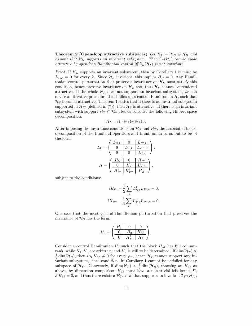
Theorem 2 (Open-loop attractive subspaces) Let HI = HS ⊕ HR andassume that HS supports an invariant subsystem. Then IS(HI) can be madeattractive by open-loop Hamiltonian control iff IR(HI) is not invariant.

Proof. If HR supports an invariant subsystem, then by Corollary 1 it must beLP,k = 0 for every k. Since HS invariant, this implies HP = 0. Any Hamil-tonian control perturbation that preserves invariance on HS must satisfy thiscondition, hence preserve invariance on HR too, thus HS cannot be renderedattractive. If the whole HR does not support an invariant subsystem, we candevise an iterative procedure that builds up a control Hamiltonian Hc such thatHS becomes attractive. Theorem 1 states that if there is no invariant subsystemsupported in HR′ (defined in (7)), then HS is attractive. If there is an invariantsubsystem with support HT ⊂ HR′ , let us consider the following Hilbert spacedecomposition:

HI = HS ⊕HT ⊕HZ .

After imposing the invariance conditions on HS and HT , the associated block-decomposition of the Lindblad operators and Hamiltonian turns out to be ofthe form:

Lk =

LS,k 0 LP ′,k

0 LT,k LP ′′,k

0 0 LZ,k

,

H =

HS 0 HP ′

0 HT HP ′′

H†P ′ H

†P ′′ HZ

,

subject to the conditions:

iHP ′ − 1

2

∑

k

L†S,kLP ′,k = 0,

iHP ′′ − 1

2

∑

k

L†T,kLP ′′,k = 0.

One sees that the most general Hamiltonian perturbation that preserves theinvariance of HS has the form:

Hc =

H1 0 00 H2 HM

0 H†M H3

.

Consider a control Hamiltonian Hc such that the block HM has full column-rank, while H1, H3 are arbitrary and H2 is still to be determined. If dim(HT ) ≤1

2dim(HR), then iρTHM 6= 0 for every ρT , hence HT cannot support any in-

variant subsystem, since conditions in Corollary 1 cannot be satisfied for anysubspace of HT . Conversely, if dim(HT ) > 1

2dim(HR), choosing an HM as

above, by dimension comparison HM must have a non-trivial left kernel K,KHM = 0, and thus there exists a HT ′ ⊂ K that supports an invariant IT ′(HI),

11

whose dimension is strictly lesser than dimension of dim(HT ). We can iteratethe reasoning with a new, refined decomposition HI = HS ⊕HT ′ ⊕ HZ′ , withHZ′ = HZ ⊕ (HT ⊖ HT ′). With this decomposition, the generator matricesexhibits the same block structure as above, with dim(HT ′ ) < dim(HT ). Thus,we can exploit the freedom of choice on the block H2 to further reduce thedimension of the invariant set. At each iteration, the procedure either stopsrendering HS attractive, if dim(HT ) ≤ 1

2dim(HR), or decrease the dimension

of the invariant set by at least 1. The procedure thus ends in at most dim(HR′ )steps. �

Remarkably, the proof of the above theorem, combined with a strategy tofind invariant subspaces, provides a constructive procedure to build a constantHamiltonian that makes the desired invariant subspace attractive whenever theTheorem’s hypothesis are satisfied.

4.2 Markovian feedback control

The potential of Hamiltonian compensation for controlling Markovian evolutionsis clearly limited by the impossibility to directly modify the noise action. Toour scopes, open-loop control is then mostly devoted to connect subspaces in Hthat are already invariant, and to adjust the generator parameters so that theinterplay between Hamiltonian and dissipative contributions (as in Eq. (5)) canstabilize the desired subspace or subsystem.

A way to overcome these limitations is offered by closed-loop control strate-gies. Measurement-based feedback control requires the ability to both effectivelymonitor the environment, and condition the target evolution upon the measure-ment record. Feedback strategies have been considered since the beginning ofthe quantum control field [28], and successfully employed in a wide variety ofsettings (see e.g. [29, 30, 24, 31, 32]).

We focus on a measurement scheme which mimics optical homo-dyne de-tection for field-quadrature measurements, whereby the target system (e.g. anatomic cloud trapped in an optical cavity) is indirectly monitored via measure-ments of the outgoing laser field quadrature [29, 33]. The conditional dynamicsof the state is stochastic, driven by the fluctuation one observes in the measure-ment. Considering a suitable infinitesimal feedback operator determined by afeedback Hamiltonian F , and taking the expectation with respect to the noisetrajectories, this leads to the Wiseman-Milburn Markovian Feedback Masterequation (FME) [29, 30]:

ρt = −i~[

H +1

2(FM +M †F ), ρt

]

+ D(M − iF, ρt). (10)

The feedback state-stabilization problem for Markovian dynamics has beenextensively studied for a single two-level system (qubit) [34, 35]. The stan-dard approach is to to design a Markovian feedback loop by assigning boththe measurement and feedback operators M,F, and to treat the measurementstrength and the feedback gain as the relevant control parameters accordingly.

12

Throughout the following section, we will assume to have more freedom, by con-sidering, for a fixed measurement operator M , both F and H as tunable controlHamiltonians

Definition 6 (CHC) A controlled FME of the form (10) supports completeHamiltonian control (CHC) if (i) arbitrary feedback Hamiltonians F ∈ H(HI)may be enacted; (ii) arbitrary constant control perturbations Hc ∈ H(HI) maybe added to the free Hamiltonian H.

This leads to both new insights and constructive control protocols for sys-tems where the noise operator is a generalized angular momentum-type observ-able, for generic finite-dimensional systems. Physically, the CHC assumptionmust be carefully scrutinized on a case by case basis, since constraints on theform of the Hamiltonian with respect to the Lindblad operator may emerge,notably in the abovementioned weak-coupling limit derivations of Markovianmodels [3].

We now address the general subspace-stabilization problem for controlledMarkovian dynamics described by FMEs. A characterization of the subspacessupporting stabilizable subsystems is provided by the following:

Theorem 3 (Feedback attractive subspaces) Let HI = HS⊕HR, with ΠS

being the orthogonal projection on HS . Assume CHC capabilities. Then, for anymeasurement operator M , there exist a feedback Hamiltonian F and a Hamilto-nian compensation Hc that make the subsystem supported by HS attractive forthe FME (10) iff

[ΠS , (M +M †)] 6= 0. (11)

Proof. Write M = MH + iMA, with both MH and MA being Hermitian, thusL = MH + i(MA−F ). Condition (11) holds iff MH is not block-diagonal whenpartitioned according to the chosen decomposition. If MH is block-diagonal,then, by Corollary 1, enforcing invariance of the subsystem supported by HS

requires that LQ = 0. But then it must also be LP = 0, so that HR supports aninvariant subsystem. Since the choice of LS and LR does not affect invariance, byTheorem 2 it follows that HS cannot be made attractive by Hamiltonian control.On the other hand, if MH is not block-diagonal, we can always find F in sucha way that L is upper diagonal, LP 6= 0, by choosing FP = iMH

P +MAP . With

L as the new noise operator, we now have to devise a control Hamiltonian Hc

with a block Hc,P that makes HS invariant (this is always possible by Corollary1, since LQ=0), and a block Hc,R constructed following the procedure in theproof of Theorem 2. �

The following specialization to pure states, i.e. one-dimensional subspaces,is immediate:

Corollary 2 Assume CHC. For any measurement operator M , there exist afeedback Hamiltonian F and a Hamiltonian compensation Hc able to stabilizean arbitrary desired pure state ρd for the FME (10) iff

[ρd, (M +M †)] 6= 0. (12)

13

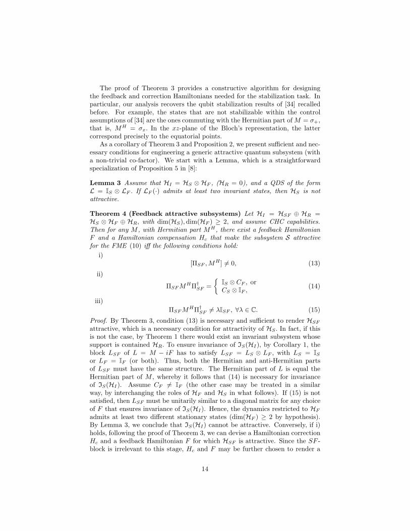
The proof of Theorem 3 provides a constructive algorithm for designingthe feedback and correction Hamiltonians needed for the stabilization task. Inparticular, our analysis recovers the qubit stabilization results of [34] recalledbefore. For example, the states that are not stabilizable within the controlassumptions of [34] are the ones commuting with the Hermitian part ofM = σ+,

that is, MH = σx. In the xz-plane of the Bloch’s representation, the lattercorrespond precisely to the equatorial points.

As a corollary of Theorem 3 and Proposition 2, we present sufficient and nec-essary conditions for engineering a generic attractive quantum subsystem (witha non-trivial co-factor). We start with a Lemma, which is a straightforwardspecialization of Proposition 5 in [8]:

Lemma 3 Assume that HI = HS ⊗ HF , (HR = 0), and a QDS of the formL = IS ⊗ LF . If LF (·) admits at least two invariant states, then HS is notattractive.

Theorem 4 (Feedback attractive subsystems) Let HI = HSF ⊕ HR =HS ⊗ HF ⊕ HR, with dim(HS), dim(HF ) ≥ 2, and assume CHC capabilities.Then for any M , with Hermitian part MH, there exist a feedback HamiltonianF and a Hamiltonian compensation Hc that make the subsystem S attractivefor the FME (10) iff the following conditions hold:

i)[ΠSF ,M

H ] 6= 0, (13)

ii)

ΠSFMHΠ†

SF =

{

IS ⊗ CF , orCS ⊗ IF ,

(14)

iii)

ΠSFMHΠ†

SF 6= λISF , ∀λ ∈ C. (15)

Proof. By Theorem 3, condition (13) is necessary and sufficient to render HSF

attractive, which is a necessary condition for attractivity of HS . In fact, if thisis not the case, by Theorem 1 there would exist an invariant subsystem whosesupport is contained HR. To ensure invariance of IS(HI), by Corollary 1, theblock LSF of L = M − iF has to satisfy LSF = LS ⊗ LF , with LS = IS

or LF = IF (or both). Thus, both the Hermitian and anti-Hermitian partsof LSF must have the same structure. The Hermitian part of L is equal theHermitian part of M , whereby it follows that (14) is necessary for invarianceof IS(HI). Assume CF 6= IF (the other case may be treated in a similarway, by interchanging the roles of HF and HS in what follows). If (15) is notsatisfied, then LSF must be unitarily similar to a diagonal matrix for any choiceof F that ensures invariance of IS(HI). Hence, the dynamics restricted to HF

admits at least two different stationary states (dim(HF ) ≥ 2 by hypothesis).By Lemma 3, we conclude that IS(HI) cannot be attractive. Conversely, if i)holds, following the proof of Theorem 3, we can devise a Hamiltonian correctionHc and a feedback Hamiltonian F for which HSF is attractive. Since the SF -block is irrelevant to this stage, Hc and F may be further chosen to render a

14

pure state of HF attractive for the reduced dynamics. Assume ii) and iii), withCF different from a scalar matrix (again, to treat the other case, CS 6= λIS , itsuffices to switch the appropriate subscripts in what follows). Thus, there existsa one-dimensional projector ρ1 such that [ρ1, CF ] 6= 0. By Corollary 2, we canfind FF and HF that render it attractive. By choosing an Hamiltonian controlso that HSF = IS ⊗ HF , and FSF = IS ⊗ FF , the stated conditions are alsosufficient for the existence of attractivity-ensuring controls. �

5 Applications

The following examples will serve to exemplify the application of our stabiliza-tion results to prototypical finite-dimensional control systems, which are also ofdirect relevance to quantum information devices. Different scenarios may arisedepending on whether the target system is (or is regarded as) indecomposable,or explicit reference to a decomposition into subsystems is made.

5.1 Single systems

Example 1: Consider a single qubit on H ≃ C2, with uncontrolled dynamicsspecified by H = n0I2 + nxσx + nyσy + nzσz, with n0, nx, ny, nz ∈ R andM = ~

2σx. Assume we wish to stabilize ρd = diag(1, 0). Since [ρd, σx] 6= 0, this

is possible. Following the procedure in the above proof, consider F = −~

2σy, so

that

L = ~σx + iσy

2= ~σ+ = ~

(

0 10 0

)

,

and Hc = −nxσx−nyσy. Substituting in the FME (10), one obtains the desiredresult, as it can also be directly verified by using Proposition 7 in [8].

Assume, more generally, that it is possible to continuously monitor an arbi-trary single-spin observable, ~σ · ~n. Since the choice of the reference frame forthe spin axis is conventional, by suitably adjusting the relative orientation ofthe measurement apparatus and the sample, it is then in principle possible toprepare and stabilize any desired pure state with a similar control strategy.

Example 2: Consider a three-level system (a qutrit), whose Hilbert spaceH ≃ C2 carries a spin-1 representation of spin angular momentum observablesJα, α = x, y, z. Without loss of generality, we may choose a basis in H suchthat the desired pure state to be stabilized is ρd = diag(1, 0, 0), and by CHC wemay also ensure that H = 0. In analogy with Example 1, a natural strategy isto continuously monitor a non-diagonal spin observable, for instance:

Jx =~√2

0 1 01 0 10 1 0

.

Since [ρd, Jx] 6= 0, the state is stabilizable. Choosing the feedback Hamiltonian

15

as

F = −Jy = − ~√2

0 −i 0i 0 −i0 i 0

,

yields

L = Jx + iJy =~√2

0 1 00 0 10 0 0

.

Unlike the qubit case, H ′ = 1

2(FM +M †F ) 6= 0, thus a Hamiltonian compensa-

tion Hc is needed to ensure that i(H ′+Hc)P − 1

2L†SLP = 0. With these choices,

it is easy to see that HR′ does not support any invariant subsystem, hence ρdis attractive.

Provided that a similar structure of the observables is ensured, the previousexamples naturally extend to generic d-level systems, as formally established in[8] by using Lyapunov techniques.

5.2 Bipartite systems

If a multipartite structure is specified on H, it is both conceptually and practi-cally important to understand whether stabilization of physically relevant classof states (including non-classical entangled states) is achievable with control re-sources which respect appropriate operational constraints, such as locality. Wefocus here on the simplest setting offered by bipartite qubit systems, with em-phasis on Markovian-feedback preparation of entangled states, which has alsobeen recently analyzed within a quantum filtering approach in [36].

Example 3: Consider a two-qubit system defined on a Hilbert space H ≃C2 ⊗C2, with a preferred basis C = {|ab〉 = |a〉⊗ |b〉 | a, b = 0, 1} (e.g., C definesthe computational basis in quantum information applications). The control taskis to engineer a QDS generator that stabilizes the maximally entangled “catstate”:

ρd =1

2(|00〉 + |11〉)(〈00|+ 〈11|).

In order to employ the synthesis techniques developed above, we consider achange of basis such that in the new representation ρd = diag(1, 0, 0, 0). Aparticularly natural choice is to consider the so-called Bell basis:

B =

{

1√2(|00〉 + |11〉), 1√

2(|00〉 − |11〉),

1√2(|01〉 + |10〉), 1√

2(|01〉 − |10〉)

}

.

Let U be the unitary matrix realizing the change of basis. In the Bell basis,which we use to build our controller, we consider a Hilbert space decompositionH = HS ⊕ HR, where HS = span{ 1√

2(|00〉 + |11〉)}, and HR = H⊥

S , and the

associated matrix block decomposition.

16

Let us consider M = σz ⊗ I in the canonical basis. It is easy to verify that[M,ρd] 6= 0. In the Bell basis, MB = UMU † = I ⊗ σx, and MP = (0, 1, 0, 0). If,in this basis, we are able to implement the feedback Hamiltonian FB = I ⊗ σy(where now the tensor product should simply be meant as a matrix operation),we render ρd invariant, yet obtaining LB = MB − iFB with LBP 6= 0. Directcomputation yields F = U †(I ⊗ σy)U = σy ⊗ σx, back in the computationalbasis. With this choice, using the definitions in the proof of Theorem 2, wehave:

HR′ = span

{

1√2(|01〉 + |10〉), 1√

2(|01〉 − |10〉)

}

,

and HR′ is itself invariant. Hence, we need to produce a control Hamiltonian Hc

to “destabilize” HR′ . By inspection, we find that HR′ contains a proper subspaceHT = span{ 1√

2(|01〉+ |10〉)} that supports an invariant and attractive state for

the dynamics reduced to HR′ . To “connect” this state to the attractive domainof ρd, we need a non-trivial Hamiltonian coupling between 1√

2(|00〉 − |11〉) and

1√2(|01〉+ |10〉). This may be obtained by a control Hamiltonian Hc = σy ⊗ I +

I ⊗ σy in the standard basis – which completes the specification of the controlstrategy that renders ρd the unique attractive state for the dynamics. Noticethat both the measurement and Hamiltonian compensation can be implementedlocally, which may be advantageous in practice.

This example suggests how our results, obtained under CHC assumptions,may be interesting to explore the compatibility with existing control constraints.A further illustration comes from the following example.

Example 4: Consider again the above two-qubit system, but now imaginethat we can only implement “non-selective” measurement and control Hamil-tonians, i.e., M,F,H must commute with the operation that swaps the qubitstates. It is then natural to restrict attention to the dynamics in the three-dimensional subspace generated by the triplet states, which correspond to eigen-value ~2J(J + 1), J = 1, of the total spin angular momentum Jα = ~

2(σα ⊗ I +

I ⊗ σα), α = x, y, z [10]:

HJ=1 = span

{

|00〉, 1√2(|01〉 + |10〉), |11〉

}

.

Notice that HJ=1 corresponds to the fixed subspace with respect to the swapoperation.

Our goal is to engineer a FME such that the maximally entangled stateρd = 1

2(|01〉 + |10〉)(〈01| + 〈10|) is attractive for the dynamics restricted to

HJ=1. Consider a collective measurement of spin along the x-axis, described byJx. Upon reordering the triplet vectors so that in the new (primed) basis thez-projection ranges over 0, 1,−1 and ρd = diag(1, 0, 0), we have:

J ′x =

~√2

0 1 11 0 01 0 0

.

17

Thus, in this basis we are looking for a feedback Hamiltonian of the form:

F ′ =~√2

0 i i

−i 0 0−i 0 0

,

that is, F ′ corresponds to the non-selective operator F = 1

~(JzJy+JyJz). Hence,

by choosing M ′ = Jx and F ′ as above we get:

L′ = M ′ − iF ′ =√

2~

0 1 10 0 00 0 0

.

This, with a choice ofH ′c = Jz suffices to make ρd attractive. In fact, considering

the Hilbert space decomposition HJ=1 = HS⊕HR, where HS = span{ 1√2(|01〉+

|10〉)}, and HR = H⊥S , we find that the largest invariant subset in HR has

support in HR′ = span{ 1√2(|00〉 − |11〉)}. By observing that 1√

2(|00〉 − |11〉) is

not an eigenstate of Jz , we infer that the chosen control parameters make ρdattractive in HJ=1.

6 Conclusion

We have revisited the fundamental concepts of invariance and attractivity forquantum Markovian subsystems from a system-theoretic viewpoint. Building onthe characterization of invariant subsystems and some partial results presentedin [8], a linear-algebraic approach and Lyapunov’s stability theory methods haveprovided us with an explicit characterization of attractive subspaces, along withan explicit attractivity test. In the special case of a single pure state, our resultsdirectly characterize the semigroup generators which support state-preparationvia dissipative Markovian dynamics.

In the second part of the work, the conditions identified for subsystem in-variance and attractivity have been exploited for designing Hamiltonian andoutput-feedback Markovian control strategies which actively achieve the in-tended quantum stabilization. In addition to a complete characterization ofsubspaces and subsystems that can be rendered attractive, our results includeconstructive recipes for synthesizing the required control parameters, which havebeen illustrated in simple yet paradigmatic examples. While our present analy-sis assumes perfect detection efficiency, a perturbative argument confirms thatunique attractive states depend in a continuous fashion on the model parameters[8].

Further work is needed in order to establish feedback stabilization resultswhich include finite bandwidth and detection efficiency, as well as simultaneousmonitoring of multiple observables. In addition, the analysis of Markovian sta-bilization problems in the presence of control resources different and/or moreconstrained than assumed here appears especially well worth pursuing. Forinstance, as illustrated in the last examples, one may want to limit possible

18

operations to local or collective observables of multipartite systems in varioussettings of physical relevance. The latter may include opto-mechanical systems,for which feedback control strategies based on homodyne detection have beenconsidered before [37], or non-equilibrium many-body systems, for which prepa-ration of a class of entangled states using “quasi-local” Markovian dissipationhas recently being investigated in a physically motivated setting [38]. Additionalinvestigation is also required to establish the full potential of Hamiltonian con-trol and Markovian feedback in synthesizing not only invariant and attractive,but also noiseless structures [8]. This may point to yet new venues for producingprotected realizations of quantum information in physical systems described byquantum Markovian semigroups.

References

[1] E. Knill. On protected realization of quantum information. Physical ReviewA, 74(4):042301:1–11, 2006.

[2] E. Knill, R. Laflamme, and L. Viola. Theory of quantum error correctionfor general noise. Physical Review Letters, 84(11):2525–2528, 2000.

[3] R. Alicki and K. Lendi. Quantum Dynamical Semigroups and Applications.Springer-Verlag, Berlin, 1987.

[4] H. P. Breuer and F. Petruccione. The Theory of Open Quantum Systems.Oxford University Press, UK, 2006.

[5] C. Altafini. Controllability properties for finite dimensional quantummarkovian master equations. Journal of Mathematical Physics, 44:2357–2372, 2003.

[6] L. Viola, E. Knill, and S. Lloyd. Dynamical decoupling of open quantumsystem. Physical Review Letters, 82(12):2417–2421, 1999.

[7] S. Lloyd and L. Viola. Engineering quantum dynamics. Physical ReviewA, 65:010101:1–4, 2001.

[8] F. Ticozzi and L. Viola. Quantum Markovian subsystems: Invariance,attractivity and control. 2008. To appear in the IEEE Transaction onAutomatic Control, on-line preprint: http://aps.arxiv.org/abs/0705.1372.

[9] L. Viola and F. Ticozzi. Attractive quantum subsystems and feedback-stabilization problems. November 2007. PHYSCON 07 conference. Avail-able on-line: http://lib.physcon.ru/?item=1317.

[10] J. J. Sakurai. Modern Quantum Mechanics. Addison-Wesley, New York,1994.

[11] E. B. Davies. Quantum Theory of Open Systems. Academic Press, USA,1976.

19

[12] G. Lindblad. On the generators of quantum dynamical semigroups. Com-munication in Mathematical Physics, 48(2):119–130, 1976.

[13] V. Gorini, A. Frigerio, M. Verri, A. Kossakowski, and E. C. G. Sudarshan.Properties of quantum markovian master equations. Reports on Mathemat-ical Physics, 13(2):149–173, 1978.

[14] K. Kraus. States, Effects, and Operations: Fundamental Notions of Quan-taum Theory. Lecture notes in Physics. Springer-Verlag, Berlin, 1983.

[15] V. Gorini, A. Kossakowski, and E.C.G. Sudarshan. Completely positivedynamical semigroups of n-level systems. Journal of Mathematical Physics,17(5):821–825, 1976.

[16] R. Blume-Kohout, H. K. Ng, D. Poulin, and L. Viola. The structureof preserved information in quantum processes. Physical Review Letters,100:030501:1–4, 2008.

[17] A. Shabani and D. A. Lidar. Theory of initialization-free decoherence-freesubspaces and subsystems. Physical Review A, 72(4):042303:1–14, 2005.

[18] H. Spohn. An algebraic condition for the approach to equilibrium of anopen n-level quantum system. Letters in Mathematical Physics, 2:33–38,1977.

[19] H. Spohn. Approach to equilibrium for completely positive dynamical semi-groups of n-level system. Reports on Mathematical Physics, 10(2):189–194,1976.

[20] H. K. Khalil. Nonlinear Systems. Prentice Hall, USA, third edition, 2002.

[21] J. F. Poyatos, J. I. Cirac, and P. Zoller. Quantum reservoir engineeringwith laser cooled trapped ions. Physical Review Letters, 77(23):4728–4731,1996.

[22] A. R. R. Carvalho, P. Milman, R. L. de Matos Filho, and L. Davidovich.Decoherence, pointer engineering, and quantum state protection. PhysicalReview Letters, 86(22):4988–4991, 2001.

[23] R. L. de Matos Filho and W. Vogel. Engineering the hamiltonian of atrapped atom. Physical Review A, 58(3):R1661–R1664, 1998.

[24] A. C. Doherty and K. Jacobs. Feedback control of quantum systems usingcontinuous state estimation. Physical Review A, 60(4):2700–2711, 1999.

[25] R. van Handel, J. K. Stockton, and H. Mabuchi. Feedback control of quan-tum state reduction. IEEE Transaction on Automatic Control, 50(6):768–780, 2005.

[26] C. Altafini. Coherent control of open quantum dynamical systems. PhysicalReview A, 70(6):062321:1–8, 2004.

20

[27] S. G. Schirmer, H. Fu, and A. I. Solomon. Complete controllability ofquantum systems. Physical Review A, 63:063410:1–8, 2001.

[28] V. P. Belavkin. Towards the theory of control in observable quantum sys-tems. Automatica and Remote Control, 44:178–188, 1983.

[29] H. M. Wiseman and G. J. Milburn. Quantum theory of optical feedbackvia homodyne detection. Physical Review Letters, 70(5):548–551, 1993.

[30] H. M. Wiseman. Quantum theory of continuous feedback. Physical ReviewA, 49(3):2133–2150, 1994.

[31] J. M. Geremia, J. K. Stockton, and H. Mabuchi. Real-time quantum feed-back control of atomic spin-squeezing. Science, 304(5668):270–273, 2004.

[32] F. Ticozzi and L. Viola. Single-bit feedback and quantum dynamical de-coupling. Physical Review A, 74(5):052328:1–11, 2006.

[33] L. K. Thomsen, S. Mancini, and H. M. Wiseman. Continuous quantumnondemolition feedback and unconditional atomic spin squeezing. Journalof Physics B, 35(23):4937–4952, 2002.

[34] J. Wang and H. M. Wiseman. Feedback-stabilization of an arbitrary purestate of a two-level atom. Physical Review A, 64(6):063810:1–9, 2001.

[35] H. M. Wiseman, S. Mancini, and J. Wang. Bayesian feedback versus marko-vian feedback in a two-level atom. Physical Review A, 66(1):013807:1–9,2002.

[36] N. Yamamoto, K. Tsumura, and S. Hara. Feedback control of quantumentanglement in a two-spin system. Automatica, 43:981–992, 2007.

[37] S. Mancini, D. Vitali, and P. Tombesi. Optomechanical cooling of amacroscopic oscillator by homodyne feedback. Physical Review Letters,80(4):688–691, 1998.

[38] B. Kraus, S. Diehl, A. Micheli, A. Kantian, H. P. Buchler, and P. Zoller.Preparation of entangled states by dissipative quantum markov processes.arXiv:quant-ph/0803.1463, 2008.

21