A General Theory of Markovian Time

Inconsistent Stochastic Control

Problems ∗

Tomas Bjork,Department of Finance,

Stockholm School of Economics,

e-mail: tomas.bjork@hhs.se

Agatha Murgoci,Department of Finance,

Copenhagen Business School,

e-mail: avm.fi@cbs.dk

September 17, 2010

First version July 13, 2008

Abstract

We develop a theory for stochastic control problems which, in vari-ous ways, are time inconsistent in the sense that they do not admit aBellman optimality principle. We attach these problems by viewing themwithin a game theoretic framework, and we look for Nash subgame per-fect equilibrium points. For a general controlled Markov process and afairly general objective functional we derive an extension of the standardHamilton-Jacobi-Bellman equation, in the form of a system of non-linearequations, for the determination for the equilibrium strategy as well asthe equilibrium value function. All known examples of time inconsistencyin the literature are easily seen to be special cases of the present theory.We also prove that for every time inconsistent problem, there exists anassociated time consistent problem such that the optimal control and theoptimal value function for the consistent problem coincides with the equi-librium control and value function respectively for the time inconsistentproblem. We also study some concrete examples.

Key words: Time consistency, time inconsistent control, dynamic pro-gramming, time inconsistency, stochastic control, hyperbolic discounting, mean-variance, Bellman equation, Hamilton-Jacobi-Bellman.

∗The authors are greatly indebted to Ivar Ekeland, Ali Lazrak, Traian Pirvu, SuleymanBasak, Mogens Steffensen, and Eric Bose-Wolf for very helpful comments.

1

Contents

1 Introduction 31.1 Dynamic programming and time consistency . . . . . . . . . . . 31.2 Three disturbing examples . . . . . . . . . . . . . . . . . . . . . . 41.3 Approaches to handle time inconsistency . . . . . . . . . . . . . . 51.4 Previous literature . . . . . . . . . . . . . . . . . . . . . . . . . . 71.5 Contributions of the present paper . . . . . . . . . . . . . . . . . 81.6 Structure of the paper . . . . . . . . . . . . . . . . . . . . . . . . 9

2 Discrete time 102.1 Setup . . . . . . . . . . . . . . . . . . . . . . . . . . . . . . . . . 102.2 Basic problem formulation . . . . . . . . . . . . . . . . . . . . . . 122.3 The game theoretic formulation . . . . . . . . . . . . . . . . . . . 132.4 The extended Bellman equation . . . . . . . . . . . . . . . . . . . 14

2.4.1 The recursion for Jn(x,u) . . . . . . . . . . . . . . . . . . 142.4.2 The recursion for Vn(x) . . . . . . . . . . . . . . . . . . . 162.4.3 Explicit time dependence . . . . . . . . . . . . . . . . . . 202.4.4 The general case . . . . . . . . . . . . . . . . . . . . . . . 222.4.5 A scaling result . . . . . . . . . . . . . . . . . . . . . . . . 23

3 Example: Non exponential discounting 233.1 A general discount function . . . . . . . . . . . . . . . . . . . . . 243.2 Hyperbolic discounting . . . . . . . . . . . . . . . . . . . . . . . . 26

4 Continuous time 274.1 Setup . . . . . . . . . . . . . . . . . . . . . . . . . . . . . . . . . 274.2 Basic problem formulation . . . . . . . . . . . . . . . . . . . . . . 284.3 The extended HJB equation . . . . . . . . . . . . . . . . . . . . . 29

4.3.1 Deriving the equation . . . . . . . . . . . . . . . . . . . . 304.3.2 The general case . . . . . . . . . . . . . . . . . . . . . . . 324.3.3 A simple special case . . . . . . . . . . . . . . . . . . . . . 344.3.4 A scaling result . . . . . . . . . . . . . . . . . . . . . . . . 354.3.5 A Verification Theorem . . . . . . . . . . . . . . . . . . . 37

5 An equivalent time consistent problem 40

6 Example: Non exponential discounting 41

7 Example: Mean-variance control 447.1 The simplest case . . . . . . . . . . . . . . . . . . . . . . . . . . . 447.2 A point process extension . . . . . . . . . . . . . . . . . . . . . . 47

8 Example: The time inconsistent linear quadratic regulator 51

9 Conclusion and future research 54

2

1 Introduction

In a standard continuous time stochastic optimal control problem the object isthat of maximizing (or minimizing) a functional of the form

E

[∫ T

0

C (s,Xs, us) ds + F (XT )

].

where X is some controlled Markov process, us is the control applied at times, and F , C are given functions. A typical example is when X is a controlledscalar SDE of the form

dXt = µ(Xt, ut)dt + σ(Xt, ut)dWt,

with some initial condition X0 = x0. Later on in the paper we will allow formore general dynamics than those of an SDE, but in this informal section werestrict ourselves for simplicity to the SDE case.

1.1 Dynamic programming and time consistency

A standard way of attacking a problem like the one above is by using DynamicProgramming (henceforth DynP). We restrict ourselves to control laws, i.e.,the control at time s, given that Xs = y, is of the form u(s, y) where the controllaw u is a deterministic function. We then embed the problem above in a familyof problems indexed by the initial point. More precisely we consider, for every(t, x), the problem Pt,x of maximizing

Et,x

[∫ T

t

C (s,Xs, us) ds + F (XT )

].

given the initial condition Xt = x. Denoting the optimal control law for Pt,x byutx(s,Xs) and the corresponding optimal value function by V (t, x) we see thatthe original problem corresponds to the problem P0,x0 .

We note that ex ante the optimal control law utx(s,Xs) for the problemPt,x must be indexed by the initial point (t, x). However, problems of the kinddescribed above turn out to be time consistent in the sense that we have theBellman optimality principle, which roughly says that the optimal controlis independent of the initial point. More precisely: if a control law is optimalon the full time interval [0, T ], then it is also optimal for any subinterval [t, T ].Given the Bellman principle, it is easy to informally derive the Hamilton-Jacobi-Bellman (henceforth HJB) equation

∂V

∂t(t, x) + sup

u

{C(t, x, u) + µ(t, x, u)

∂V

∂x(t, x)

12σ2(t, x, u)

∂2V

∂x2(t, x)

}= 0,

V (T, x) = F (x),

for the determination of V . One can (with considerable effort) show rigorouslythat, given enough regularity, the optimal value function will indeed satisfy the

3

HJB equation. On can also (quite easily) prove a verification theorem whichsays that if V is a solution of the HJB equation, then V is indeed the optimalvalue function for the control problem, and the optimal control law is given bythe maximizing u in the HJB equation.

We end this section by listing some important points concerning time con-sistency.

Remark 1.1 The main reasons for the time consistency of the problem aboveare as follows.

• The integral term C (s,Xs, us) in the problem Pt,x is allowed to dependon s, Xs and us. It is not allowed to depend on the initial point (t, x).

• The terminal evaluation term is allowed to be of the form Et,x [F (XT )], i.ethe expected value of a non-linear function of the terminal value XT . Timeconsistency is then a relatively simple consequence of the law of iteratedexpectations. We are not allowed to have a term of the form G(Et,x [XT ]),which is a non-linear function of the expected value.

• We are not allowed to let the terminal evaluation function F depend onthe initial point (t, x).

1.2 Three disturbing examples

We will now consider three seemingly simple examples from financial economics,where time consistency fail to hold. In all these cases we consider a standardBlack-Scholes model for an underlying stock price S, as well as a bank accountB with short rate r.

dSt = αStdt + σStdWt,

dBt = rBtdt.

We consider a self financing portfolio based on S and B where ut is the numberof dollars invested in the risky asset S, and c is the consumption rate at time t.Denoting the market value process of this portfolio by X, we have

dXt = [rXt + (α− r)ut − ct]dt + σutdWt,

and we now consider three indexed families of optimization problems. In allcases the (naive) objective is to maximize the objective functional J(t, x,u),where (t, x) is the initial point and u is the control law.

1. Hyperbolic discounting

J(t, x,u) = Et,x

[∫ T

t

ϕ(s− t)h(cs)dt + ϕ(T − t)F (XT )

]In this problem h is the local utility of consumption, F is the utilityof terminal wealth, and ϕ is the discounting function. This problem

4

differs from a standard problem by the fact that the initial point in timet enters in the integral (see Remark 1.1). Obviously; if ϕ is exponentialso ϕ(s− t) = e−a(s−t then we can factor out eat and convert the probleminto a standard problem with objective functional

J(t, x,u) = Et,x

[∫ T

t

e−ash(cs)dt + e−aT F (XT )

]One can show, however, that every choice of the discounting functionϕ, apart from the the exponential, case, will lead to a time inconsistentproblem. More precisely, the Bellman optimality principle will not hold.

2. Mean variance utility

J(t, x,u) = Et,x [XT ]− γ

2V art,x (XT )

This case is a continuous time version of a standard Markowitz investmentproblem where we want to maximize utility of final wealth. The utility offinal wealth is basically linear in wealth, as given by the term Et,x [XT ],but we penalize the risk by the conditional variance γ

2 V art,x (XT ). Thislooks innocent enough, but we recall the elementary formula

V ar[X] = E[X2]− E2[X].

Now, in a standard time consistent problem we are allowed to have termslike Et,x [F (XT )] in the objective functional, i.e. we are allowed to havethe expected value of a non-linear function of terminal wealth. In thepresent case, however we have the term (Et,x [X])2. This is not an ex-pected value of a non-linear function of terminal wealth, but instead anon-linear function of the expected value of terminal wealth, and we thushave a time inconsistent problem (see Remark 1.1).

3. Endogenous habit formation

J(t, x,u) = Et,x [ln (XT − x + β)] , β > 0.

In this particular example we basically want to maximize log utility ofterminal wealth. In a standard problem we would have the objectiveEt,x [ln (XT − d)] where d > 0 is the lowest acceptable level of terminalwealth. In our problem, however, the lowest acceptable level of terminalwealth is given by x−β and it thus depends on your wealth Xt = x at timet. This again leads to a time inconsistent problem. (We remark in passingthat there are other examples of endogenous habit formation which areindeed time consistent.)

1.3 Approaches to handle time inconsistency

In all the three examples of the previous subsection we are faced with a timeinconsistent family of problems, in the sense that if for some fixed initial point

5

(t, x) we determine the control law u which maximizes J(t, x,u), then at somelater point (s,Xs) the control law u will no longer be optimal for the functionalJ(s,Xs,u). It is thus conceptually unclear what we mean by “optimality” andeven more unclear what we mean by “an optimal control law”, so our first taskis to specify more precisely exactly which problem we are trying to solve. Thereare then at least three different ways of handling a family of time inconsistentproblems, like the ones above

• We dismiss the entire problem as being silly.

• We fix one initial point, like for example (0, x0), and then try to find thecontrol law u which maximizes J(0, x0,u). We then simply disregard thefact that at a later points in time such as (s,Xs) the control law u willnot be optimal for the functional J(s,Xs,u). In the economics literature,this is known as pre-commitment.

• We take the time inconsistency seriously and formulate the problem ingame theoretic terms.

All of the three strategies above may in different situations be perfectlyreasonable, but in the present paper we choose the last one. The basic idea isthen that when we decide on a control action at time t we should explicitly takeinto account that at future times we will have a different objective functionalor, in more loose terms, “our tastes are changing over time”. We can then viewthe entire problem as a non-cooperative game, with one player for each time t,where player t can be viewed as the future incarnation of ourselves (or ratherof our preferences) at time t. Given this point of view, it is natural to look forNash equilibria for the game, and this is exactly our approach.

In continuous time it is far from trivial to formulate this intuitive idea inprecise terms. We will do this in the main text below but a rough picture of thegame is as follows.

• We consider a game with one player at each point t in time. This player isreferred to as “player t”. You may think of player t as a future incarnationof yourself, but conceptually it may be easier to think of the game as beingplayed by a continuum of completely different individuals.

• Depending on t and on the position x in space, player t will choose acontrol action. This action is denoted by u(t, x), so the strategy chosenby player t is given by the mapping x 7−→ u(t, x).

• A control law u can thus be viewed as a complete description of the chosenstrategies of all players in the game.

• The reward to player t is given by the functional J(t, x,u). We note thatin the three examples of the previous section it is clear that J(t, x,u) doesnot depend on the actions taken by any player s for s < t, so in fact J doesonly depend on the restriction of the control law u to the time interval

6

[t, T ]. It is also clear that this is really a game, since the reward to playert does not only depend on the strategy chosen by himself, but also by thestrategies chosen by all players coming after him in time.

We can now loosely define the concept of a “Nash subgame perfect equilibriumpoint” of the game. This is a control law u satisfying the following condition:

• Choose an arbitrary point t in time.

• Suppose that every player s, for all s > t, will use the strategy u(s, ·).

• Then the optimal choice for player t is that he/she also uses the strategyu(t, ·).

The problem with this “definition” in continuous time is that, for example in adiffusion framework without impulse controls, the individual player t does notreally influence the outcome of the game at all. He/she only chooses the controlat the single point t, and since this is a time set of Lebesgue measure zero, thecontrol dynamics will not be influenced. For a proper definition we need somesort of limiting argument, which is given in the main text below.

1.4 Previous literature

The game theoretic approach to time inconsistency using Nash equilibriumpoints as above has a long history starting with [12] where a deterministic Ram-say problem is studied. Further work along this line in continuous and discretetime is provided in [6], [7], [9], [10], and [13].

Recently there has been renewed interest in these problems. In the interest-ing, and mathematically very advanced, papers [4] and [5], the authors consideroptimal consumption and investment under hyperbolic discounting (Problem 1in our list above) in deterministic and stochastic models from the above gametheoretic point of view. To our knowledge, these papers were the first to providea precise definition of the equilibrium concept in continuous time. The authorsderive, among other things, an extension of the HJB equation to a system ofPDEs including an integral term, and they also provide a rigorous verificationtheorem. They also, in a tour de force, derive an explicit solution for the casewhen the discounting function is a weighted sum of two exponential discountfunctions. Our present paper is much inspired by these papers, in particular forthe definition of the equilibrium law.

In [1] the authors undertake a deep study of the mean variance problemwithin a Wiener driven framework. This is basically Problem 2 in the listabove, but the authors also consider the case of multiple assets, as well asthe case of a hidden Markov process driving the parameters of the asset pricedynamics. The authors derive an extension of the Hamilton Jacobi Bellmanequation and manages, by a number of very clever ideas, to solve this equationexplicitly for the basic problem, and also for the above mentioned extensions.The paper has two limitations: Firstly, from a mathematical perspective it issomewhat heuristic, the equilibrium concept is never given a precise definition,

7

and no verification theorem is provided. Secondly, and more importantly, themethodology depends heavily on the use of a “total variance formula”, which insome sense (partially) replaces the iterated expectations formula in a standardproblem. This implies that the basic methodology cannot be extended beyondthe mean variance case. The paper is extremely thought provoking, and we havebenefited greatly from reading it.

The recent working paper [8] uses the theory of the present paper andcontains several interesting new applications. In [3] the author undertakes adeep study of the mean variance problem within in a general semi martingaleframework.

1.5 Contributions of the present paper

The object of the present paper is to undertake a rigorous study of time incon-sistent control problems in a reasonably general Markovian framework, and inparticular we do not want to tie ourselves down to a particular applied problem.We have therefore chosen a setup of the following form.

• We consider a general controlled Markov process X, living on somesuitable space (details are given below). It is important to notice thatwe do not make any structural assumptions whatsoever about X, and wenote that the setup obviously includes the case when X is determined bya system of SDEs driven by a Wiener and a point process.

• We consider a functional of the form

J(t, x,u) = Et,x

[∫ T

t

C (x,Xus ,u(Xu

s )) ds + F (x,XuT )

]+G (x,Et,x [Xu

T ]) .

We see that with the choice of functional above, time inconsistency enters atseveral different points. Firstly we have the appearance of the present statex in the local utility function C, as well as in the functions F and G. Asa consequence of this, the utility function changes as the state changes. Attime t we have, for example, the utility function F (Xt, XT ) which we wantto maximize as a function of XT , but at a later time s we have the utilityfunction F (Xs, XT ). This obviously leads to time inconsistency. Secondly, inthe term G (x,Et,x [Xu

T ]) we have, even forgetting about the appearance of x,a non linear function G acting on the conditional expectation, again leading totime inconsistency.

Note that, for notational simplicity we have not explicitly included de-pendence on running time t. This can always be done by letting running timebe one component of the state process X, so the setup above also allows forexpressions like F (t, x, Xu

T ) etc, thus allowing (among many other things) forhyperbolic discounting.

This setup is studied in some detail in continuous as well as in discretetime. The discrete time results are parallel to those in continuous time, and ourmain results in continuous time are as follows.

8

• We provide a precise definition of the Nash equlibrium concept. (This isdone along the lines of [4] and [5]).

• We derive an extension of the standard Hamilton-Jacobi-Bellman equa-tion to a non standard system of equations for the determination of theequilibrium value function V .

• We prove a verification theorem, showing that the solution of the extendedHJB system is indeed the equilibrium value function, and that the equi-librium strategy is given by the optimizer in the equation system.

• We prove that to every time inconsistent problem of the form above, thereexists an associated standard, time consistent, control problem withthe following properties:

– The optimal value function for the standard problem coincides withthe equilibrium value function for the time inconsistent problem.

– The optimal control law for the standard problem coincides with theequilibrium startegy for the time inconsistent problem.

• We solve some specific test examples.

Our framework and results extends the existing theory considerably. Aswe noted above, hyperbolic discounting is included as a special case of thetheory. The mean variance example from above is of course also included. Moreprecisely it is easy to see that it corresponds to the case when

C = 0, F (x, y) = y − γ

2y2, G (x, y) =

γ

2y2

We thus extend the existing literature by allowing for a considerably more gen-eral utility functional, and a completely general Markovian structure. The exis-tence of the associated equivalent standard control problem is to our knowledgea completely new result.

1.6 Structure of the paper

Since the equilibrium concept in continuous time is a very delicate one, we startby studying a discrete time version of our problem in Section 2. In discretetime there are no conceptual problems with the equilibrium concept, but thearguments are sometimes quite delicate, the expressions are rather complicated,and great care has to be taken. It is in fact in this section that the main workis done. In Section 3 we exemplify the theory by studying the special case ofnon exponential discounting.

In Section 4 we study the continuous time problem by taking formal limitsfor a discretized problem, and using the results of the Section 2. This leads toan extension of the standard HJB equation to a system of equations with anembedded static optimization problem. The limiting procedure described aboveis done in an informal manner and it is largely heuristic, so in order to prove

9

that the derived extension of the HJB equation is indeed the correct one wealso provide a rigorous proof of a verification theorem. In Section 5 we provethe existence of the associated standard control problem, and in Sections 6-8we study several examples.

2 Discrete time

Since the theory is conceptually much easier in discrete time than in continuoustime, we start by presenting the discrete time version.

2.1 Setup

We consider a given controlled Markov process X, evolving on a measurablestate space {X ,GX}, with controls taking values in a measurable control space{U ,GU}. The action is in discrete time, indexed by the set N of natural numbers.The intuitive idea is that if Xn = x, then we can choose a control un ∈ U , andthis control will affect the transition probabilities from Xn to Xn+1. This ideais formalized by specifying a family of transition probabilities,

{pun(dz;x) : n ∈ N, x ∈ X , u ∈ U} .

For every fixed n ∈ N, x ∈ X and u ∈ U , we assume that pun(·;x) is a proba-

bility measure on X , and for each A ∈ GX , the probability pun(A;x) is jointly

measurable in (x, u). The interpretation of this is that pun(dz;x) is the proba-

bility distribution of Xn+1, given that Xn = x, and that we at time n apply thecontrol u, i.e.,

pun(dz;x) = P (Xn+1 ∈ dz |Xn = x, un = u ) .

To obtain a Markov structure, we restrict the controls to be feedbackcontrol laws, i.e. i.e. at time n, the control un is allowed to depend on time nand state Xn. We can thus write

un = un(Xn),

where the mapping u : N×X → U is measurable. Note the boldface notationfor the mapping u. In order to distinguish between functions and functionvalues, we will always denote a control law (i.e. a mapping) by using boldface,like u, whereas a possible value of the mapping will be denoted without boldface,like, u ∈ U .

Given the family of transition probabilities we may define a correspondingfamily of operators, operating on function sequences.

Definition 2.1 A function sequence is a mapping f : N×X → R, wherewe use the notation (n, x) 7−→ fn(x).

10

• For each u ∈ U , the operator Pu, acting on the set of integrable functionsequences, is defined by

(Puf)n (x) =∫X

fn+1(z)pun(dz, x).

The corresponding discrete time “infinitesimal” operator Au is defined by

Au = Pu − I,

where I is the identity operator.

• For each control law u the operator Pu is defined by

(Puf)n (x) =∫X

fn+1(z)pun(x)n (dz, x),

and Au is defined correspondingly as

Au = Pu − I,

In more probabilistic terms we have the interpretation.

(Puf)n (x) = E [fn+1(Xn+1)|Xn = x, un = u] ,

and Au is the discrete time version of the continuous time infinitesimal operator.We immediately have the following result.

Proposition 2.1 Consider a real valued function sequence {fn(x)}, and a con-trol law u. The process fn(Xu

n ) is then a martingale under the measure inducedby u if and only if the sequence {fn} satisfies the equation

(Auf)n (x) = 0, n = 0, 1, . . . , T − 1.

Proof. Obvious from the definition of Au.

It is clear that for a fixed initial point (n, x) and a fixed control law u wemay in the obvious way define a Markov process denoted by Xn,x,u, where fornotational simplicity we often drop the upper index n, x and use the notationXu. The corresponding expectation operator is denoted by Eu

n,x [·], and weoften drop the upper index u, and instead use the notation En,x [·]. A typicalexample of an expectation will thus have the form En,x [F (Xu

k )] for some realvalued function F and some point in time k.

11

2.2 Basic problem formulation

For a fixed (n, x) ∈ N × X , a fixed control law u, and a fixed time horizon T ,we consider the functional

Jn(x,u) = En,x

[T−1∑k=n

C (x,Xuk ,uk(Xu

k )) + F (x,XuT )

]+ G (x,En,x [Xu

T ]) , (1)

Obviously, the functional J depends only on the restriction of the control lawu to the time set k = n, n + 1, . . . , T − 1.

The intuitive idea is that we are standing at (n, x) and that we would liketo choose a control law u which maximizes J . We can thus define an indexedfamily of problems {Pn,x} by

Pn,x : maxu

Jn(x,u),

where max is shorthand for the imperative “maximize!”. The complicatingfactor here is that the family {Pn,x} is time inconsistent in the sense that if uis optimal for Pn,x, then the restriction of u to the time set k, k + 1, . . . , T (fork > n) is not necessarily optimal for the problem Pk,Xu

k. There are two reasons

for this time inconsistency:

• The shape of the utility functional depends explicitly on the initial positionx in space, as can be seen in the appearance of x in the expression F (x,XT )and similarly for the other terms. In other words, as the X process movesaround, our utility function changes, so at time t this part of the utilityfunction will have the form F (Xt, XT ).

• For a standard time consistent control problem we are allowed to haveexpressions like En,x [G(XT )] in the utility function, i.e. we are allowed tohave the expected value of a non linear function G of the future processvalue. Time consistency is then a relatively simple consequence of thelaw of iterated expectations. In our problem above, however, we have anexpression of the form G (En,x [Xu

T ]), which is not the expectation of a nonlinear function, but a nonlinear function of the expected value. We thusdo not have access to iterated expectations, so the problem becomes timeinconsistent. On top of this we also have the appearance of the presentstate x in the expression G (x,En,x [Xu

T ]).

The moral of all this is that we have a family of time inconsistent problemsor, alternatively, we have time inconsistent preferences. If we at some point(n, x) decide on a feedback law u which is optimal from the point of view of(n, x) then as time goes by, we will no longer consider u to be optimal. Tohandle this problem we will, as outlined above, take a game theoretic approachand we now go on the describe this in some detail.

12

2.3 The game theoretic formulation

The idea, which appears already in [12], is to view the setup above in gametheoretic terms. More precisely we view it as a non-cooperative game wherewe have one player at each point n in time. We refer to this player as “playernumber n” and the rule is that player number n can only choose the controlun. One interpretation is that these players are different future incarnations ofyourself (or rather incarnations of your future preferences), but conceptually itis perhaps easier to think of it as one separate player at each n.

Given the data (n, x), player number n would, in principle, like to maximizeJn(x,u) over the class of feedback controls u, but since he can only choose thecontrol un, this is not possible. Instead of looking for “optimal” feedback laws,we take the game theoretic point of view and study so called subgame perfectNash equilibrium strategies. The formal definition is as follows.

Definition 2.2 We consider a fixed control law u and make the following con-struction.

1. Fix an arbitrary point (n, x) where n < T , and choose an arbitrary controlvalue u ∈ U .

2. Now define the control law u on the time set n, n+1, . . . , T −1 by setting,for any y ∈ X ,

uk(y) ={

uk(y), for k = n + 1, . . . , T − 1,u, for k = n.

We say that u is a subgame perfect Nash equilibrium strategy if, for everyfixed (n, x), the following condition hold

supu∈U

Jn(x, u) = Jn(x, u).

If an equlibrium control u exists, we define the equilibrium value functionV by

Vn(x) = Jn(x, u).

In more pedestrian terms this means that if player number n knows thatall players coming after him will use the control u, then it is optimal for playernumber n also to use un.

Remark 2.1 An equivalent, and perhaps more concrete, way of describing anequilibrium strategy is as follows.

• The equilibrium control uT−1(x) is obtained by letting player T−1 optimizeJT−1(x,u) over uT−1 for all x ∈ X . This is a standard optimizationproblem without any game theoretic components.

• The equilibrium control uT−2 is obtained by letting player T − 2 chooseuT−2 to optimize JT−2, given the knowledge that player number T −1 willuse uT−1.

13

• Proceed recursively by induction.

Obviously; for a standard time consistent control problem, the game the-oretic aspect becomes trivial and the equilibrium control law coincides withthe standard (time consistent) optimal law. The equilibrium value function Vwill coincide with the optimal value function and, using dynamic programmingarguments, V is seen to satisfy a standard Bellman equation.

The main result of the present paper is that in the time inconsistent case,the equilibrium value function V will satisfy a system of non linear equations.This system of equations extend the standard Bellman equation, and for a timeconsistent problem they reduce to the Bellman equation.

2.4 The extended Bellman equation

In this section we assume that there exists an equilibrium control law u (whichmay not be unique) and we consider the corresponding equilibrium value func-tion V defined above. The goal of this section is to derive an system of equations,extending the standard Bellman equation, for the determination of V . This willbe done in the following two steps:

• For an arbitrarily chosen control law u, we will derive a recursive equationfor Jn(x,u).

• We will then fix (n, x) and consider two control laws. The first one isthe equilibrium law u, and the other one is the law u where we chooseu = un(x) arbitrarily, but follow the law u for all k with k = n+1, . . . T−1.The trivial observation that

supu∈U

Jn(x,u) = Jn(x, u) = Vn(x),

will finally give us the extension of the Bellman equation.

The reader with experience from dynamic programming (DynP) will recoginizethat the general program above is in fact more or less the same as for stan-dard (time consistent) DynP. However; in the present time inconsistent setting,the derivation of the recursion in the first step is much more tricky than inthe corresponding step from DynP, and it also requires some completely newconstructions.

2.4.1 The recursion for Jn(x,u)

In order to derive the recursion for Jn(x,u) we consider an arbitrary initial point(n, x), and we consider an arbitrarily chosen control law u. The value taken byu at (n, x) will play a special role in the sequel, and for ease of reading we willuse the notation un(x) = u.

We now go on to derive a recursion between Jn and Jn+1. This is conceptu-ally rather delicate, and sometimes a bit messy. In order to increase readability

14

we therefore carry out the derivation only for the case when the objective func-tional does not contain the sum

∑T−1k=n C (x,Xu

k ,uk(Xuk )) in (1), and thus has

has the simpler form

Jn(x,u) = En,x [F (x,XuT )] + G (x,En,x [Xu

T ]) . (2)

We provide the result for the general case in Section 2.4.4. The derivation ofthis is completely parallel to that of the simplified case.

We start by making the observation that Xn+1 will only depend on x andon the control value un(x) = u motivating the notation Xu

n+1. The distributionof Xk for k > n + 1 will, on the other hand depend on the control law u(restricted to the interval [n, k − 1]) so for k > n + 1 we use the notation Xu

k .We now go on to the recursion arguments. From the definition of J we

have

Jn+1(Xun+1,u) = En+1

[F (Xu

n+1, XuT )

]+ G

(Xu

n+1, En+1 [XuT ]

), (3)

where for simplicity of notation we write En+1 [·] instead of En+1,Xun+1

[·]. Wenow make the following definitions which will play a central role in the sequel.

Definition 2.3 For any control law u, we define the function sequences {fun }

and {gun}, where fu

n , gun : X × X → R by.

fun (x, y) = En,x [F (y, Xu

T )] ,gu

n(x) = En,x [XuT ] .

We also introduce the notation

fu,yn (x) = fu

n (x, y).

The difference between fu,yn and fu

n , is that we view fun as a function of the

two variables x and y, whereas fu,yn is, for a fixed y, viewed as a function of the

single variable x.From the definitions above it is obvious that, for any fixed y, the processes

fu,yn (Xu

n ) and gun(Xu

n ) are martingales under the measure generated by u. Wethus have the following result.

Lemma 2.1 For every fixed control law u and every fixed choice of y ∈ X , thefunction sequence {fu,y

n } satisifes the recursion

(Aufu,y)n (x) = 0, n = 0, 1, . . . , T − 1.

fu,yT (x) = F (y, x).

The sequence {gun} satisifes the recursion

(Augu)n (x) = 0, n = 0, 1, . . . , T − 1.

guT (x) = x.

15

Going back to (3) we note that, from the Markovian structure and thedefinitions above, we have

En+1

[F (Xu

n+1, XuT )

]= fu

n+1(Xun+1, X

un+1)

En+1 [XuT ] = gu

n+1(Xun+1).

We can now write (3) as

Jn+1(Xun+1,u) = fu

n+1(Xun+1, X

un+1) + G

(Xu

n+1, gun+1(X

un+1)

).

Taking expectations gives us

En,x

[Jn+1(Xu

n+1,u)]

= En,x

[fu

n+1(Xun+1, X

un+1)

]+En,x

[G

(Xu

n+1, gun+1(X

un+1)

)],

and, going back to the definition of Jn(x,u), we can write this as

En,x

[Jn+1(Xu

n+1,u)]

= Jn(x,u)

+ En,x

[fu

n+1(Xun+1, X

un+1)

]− En,x [F (x,Xu

T )]

+ En,x

[G

(Xu

n+1, gun+1(X

un+1)

)]−G (x,En,x [Xu

T ]) .

At this point it may seem natural to use the identities En,x [F (x,XuT )] = fu

n (x, x)and En,x [Xu

T ] = gun(x), but for various reasons this is not a good idea. Instead

we note that

En,x [F (x,XuT )] = En,x [En+1 [F (x,Xu

T )]] = En,x

[fu

n+1(Xun+1, x)

],

and thatEn,x [Xu

T ] = En,x [En+1 [XuT ]] = En,x

[gu

n+1(Xun+1)

].

Substituting these identities into the recursion above, we can now collect thefindings so far.

Lemma 2.2 The value function J satisfies the following recursion.

Jn(x,u) = En,x

[Jn+1(Xu

n+1,u)]

−{En,x

[fu

n+1(Xun+1, X

un+1)

]− En,x

[fu

n+1(Xun+1, x)

]}−

{En,x

[G

(Xu

n+1, gun+1(X

un+1)

)]−G

(x,En,x

[gu

n+1(Xun+1)

])}.

2.4.2 The recursion for Vn(x)

We will now derive the fundamental equation for the determination of the equlib-rium function Vn(x). In order to do this we assume that there exists an equi-librium control u. We then fix an arbitrarily chosen initial point (n, x) andconsider two strategies (control laws).

1. The first control law is simply the equilibrium law u.

16

2. The second control law u is slightly more complicated. We choose anarbitrary point u ∈ U and then defined the control law u as follows

uk(y) ={

u, for k = n,uk(y), for k = n + 1, . . . , T − 1.

We now compare the objective function Jn for these two control laws. Firstly,and by definition, we have

Jn(x, u) = Vn(x),

where V is the equilibrium value function defined earlier. Secondly, and also bydefinition, we have

Jn(x,u) ≤ Jn(x, u),

for all choices of u ∈ U . We thus have the inequality

Jn(x,u) ≤ Vn(x),

for all u ∈ U , with equality if u = un(x). We thus have the basic relation

supu∈U

Jn(x,u) = Vn(x). (4)

We now make a small variation of Definition 3.

Definition 2.4 We define the function sequences {fn}Tn=0, and {gn}T

n=0, wherefn : X × X → R, and gn : X → R by.

fn(x, y) = En,x

[F

(y, X u

T

)],

gn(x) = En,x

[X u

T

].

We also introduce the notation

fyn(x) = fn(x, y),

where we view fyn as a function of x with y as a fixed parameter.

Using Lemma 2.2, the basic relation (4) now reads

supu∈U

{En,x

[Jn+1(Xu

n+1,u)]− Vn(x)

−(En,x

[fu

n+1(Xun+1, X

un+1)

]− En,x

[fu

n+1(Xun+1, x)

])−

(En,x

[G

(Xu

n+1, gun+1(X

un+1)

)]−G

(x,En,x

[gu

n+1(Xun+1)

]))}= 0.

W now observe that, since the control law u conicides with the equilibrium lawu on [n + 1, T − 1], we have the following equalities

Jn+1(Xun+1,u) = Vn+1

(Xu

n+1

),

fun+1(X

un+1, x) = fn+1(Xu

n+1, x),gu

n+1(Xun+1) = gn+1(Xu

n+1).

17

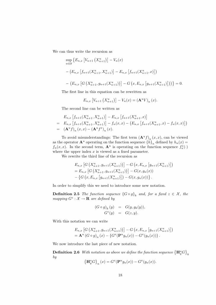
We can thus write the recursion as

supu∈U

{En,x

[Vn+1

(Xu

n+1

)]− Vn(x)

−(En,x

[fn+1(Xu

n+1, Xun+1)

]− En,x

[fn+1(Xu

n+1, x)])

−(En,x

[G

(Xu

n+1, gn+1(Xun+1)

)]−G

(x,En,x

[gn+1(Xu

n+1)]))}

= 0.

The first line in this equation can be rewritten as

En,x

[Vn+1

(Xu

n+1

)]− Vn(x) = (AuV )n (x).

The second line can be written as

En,x

[fn+1(Xu

n+1, Xun+1)

]− En,x

[fn+1(Xu

n+1, x)]

= En,x

[fn+1(Xu

n+1, Xun+1)

]− fn(x, x)−

(En,x

[fn+1(Xu

n+1, x)− fn(x, x)])

= (Auf)n (x, x)− (Aufx)n (x).

To avoid misunderstandings: The first term (Auf)n (x, x), can be viewedas the operator Au operating on the function sequence {h}n defined by hn(x) =fn(x, x). In the second term, Au is operating on the function sequence fx

n (·)where the upper index x is viewed as a fixed parameter.

We rewrite the third line of the recursion as

En,x

[G

(Xu

n+1, gn+1(Xun+1)

)]−G

(x,En,x

[gn+1(Xu

n+1)])

= En,x

[G

(Xu

n+1, gn+1(Xun+1)

)]−G(x, gn(x))

−{G

(x,En,x

[gn+1(Xu

n+1)])−G(x, gn(x))

}.

In order to simplify this we need to introduce some new notation.

Definition 2.5 The function sequence {G � g}k and, for a fixed z ∈ X , themapping Gz : X → R are defined by

(G � g)k (y) = G(y, gk(y)),Gz(y) = G(z, y).

With this notation we can write

En,x

[G

(Xu

n+1, gn+1(Xun+1)

)]−G

(x,En,x

[gn+1(Xu

n+1)])

= Au (G � g)n (x)− {Gx(Pugn(x))−Gx(gn(x))} .

We now introduce the last piece of new notation.

Definition 2.6 With notation as above we define the function sequence{Hu

gG}

kby {

HugG

}n

(x) = Gx(Pugn(x))−Gx(gn(x)).

18

Finally, we may state the main result for discrete time models.

Theorem 2.1 Consider a functional of the form (2), and assume that an equi-librium control law u exists. Then the equilibrium value function V satisfies theequation.

supu∈U

{(AuV )n (x)− (Auf)n (x, x) + (Aufx)n (x)

− Au (G � g)n (x) + HugGn(x)

}= 0, (5)

VT (x) = F (x, x) + G(x, x), (6)

where the supremum above is realized by u = un(x). Furthermore, the followinghold.

1. For every fixed y ∈ X the function sequence fyn(x) is determined by the

recursion

Aufyn(x) = 0, n = 0, . . . , T − 1, (7)

fyT (x) = F (y, x), (8)

and fn(x, x) is given by

fn(x, x) = fxn (x).

2. The function sequence gn(x) is determined by the recursion.

Augn(x) = 0, n = 0, . . . , T − 1, (9)gT (x) = x, (10)

3. The probabilistic interpretations of f and g are, as before, given by

fn(x, y) = En,x

[F

(y, X u

T

)],

gn(x) = En,x

[X u

T

].

4. In the recursions above, the u occurring in the expression Au is the equi-librium control law.

We now have some comments on this result.

• The first point to notice is that we have a system of recursion equation(5)-(10) for the simultaneous determination of V , f and g.

• In the case when F (x, y) does not depend upon x, and there is no G term,the problem trivializes to a standard time consistent problem. The terms(Auf)n (x, x)+ (Aufx)n (x) in the V -equation (5) cancel, and the systemreduces to the standard Bellman equation

(AuV )n (x) = 0,

VT (x) = F (x).

19

• In order to solve the V -equation (5) we need to know f and g but these aredetermined by the equilibrium control law u, which in turn is determinedby the sup-part of (5).

• We can view the system as a fixed point problem, where the equilibriumcontrol law u solves an equation of the form M(u) = u. The mapping Mis defined by the following procedure.

– Start with a control u.

– Generate the functions f and g by the recursions

Aufyn(x) = 0,

Augn(x) = 0,

and the obvious terminal conditions.

– Now plug these choices of f and g into the V equation and solve itfor V . The control law which realizes the sup-part in (5) is denotedby M(u). The optimal control law is determined by the fixed pointproblem M(u) = u.

This fixed point property is rather expected since we are looking for aNash equilibrium point, and it is well known that such a point is typicallydetermined as fixed points of a mapping. We also note that we can viewthe system as a fixed point problem for f and g.

• In the present discrete time setting, the situation is, however, simplerthan the fixed point argument above may lead us to believe. In fact;looking closer at the recursions, it turns out that the system for V , f , andg is a formalization of the recursive strategy outlined in Remark 2.1.

2.4.3 Explicit time dependence

In many examples, the objective functional exhibits explicit time dependence,in the sense that the functions F and G depend explicitly on running time n,so J has the form

Jn(x,u) = En,x [Fn(x,XuT )] + Gn (x,En,x [Xu

T ]) . (11)

This case is in fact included in the theory developed above by considering theextended state process (n, Xn), where n has trivial dynamics. Since problems ofthis form are quite common we nevertheless provide the result for easy reference.The novelty for this case is that the function sequence

fyn(x) = En,x

[F

(y, X u

T

)].

will be replaced by the sequence

fkyn (x) = En,x

[Fk

(y, X u

T

)].

20

Proposition 2.2 For a functional of the form (11), the following hold.

1. The equilibrium value function V satisfies the equation.

supu∈U

{(AuV )n (x)− (Auf)nn (x, x) + (Aufnx)n (x)

− Au (G � g)n (x) + HugGn(x)

}= 0, (12)

VT (x) = FT (x, x) + GT (x, x), (13)

where the supremum above is realized by u = un(x).

2. For every fixed k = 0, 1, . . . , T and every y ∈ X the function sequencefky

n (x) is determined by the recursion

Aufkyn (x) = 0, n = 0, . . . , T − 1, (14)

fkyT (x) = Fk(y, x), (15)

and fnn(x, x) is defined by

fnn(x, x) = fnxn (x).

3. The function sequence gn(x) is determined by the recursion.

Augn(x) = 0, n = 0, . . . , T − 1, (16)gT (x) = x, (17)

4. The function sequence (G � g) is defined by

(G � g)n (x) = Gn(x, gn(x))

5. The term HugGn(x) is defined by

HugGn(x) = Gn (x, Pugn(x))−Gn(x, gn(x))

6. The probabilistic interpretations of f and g are given by

fnk(x, y) = En,x

[Fk

(y, X u

T

)], (18)

gn(x) = En,x

[X u

T

]. (19)

7. In the expressions above, the u occurring in the expression Au is theequilibrium control law.

Remark 2.2 Note that for every fixed k = 0, 1, 2, . . . , T the function fnk(x, y)is defined for all n = 0, 1, 2, . . . , T , not only for n ≤ k.

21

2.4.4 The general case

We now consider the most general functional form, where J is given by

Jn(x,u) = En,x

[T−1∑k=n

Cn,k (x,Xuk ,uk(Xu

k )) + Fn(x,XuT )

]+ Gn (x,En,x [Xu

T ]) .

(20)The arguments for the C terms in the sum above are very similar to the previousarguments for the F term. It is thus natural to introduce an indexed functionsequence defined by

ck,m,yn (x) = En,x

[Ck,m

(y, X u

m, um

(X u

m

))]where, as usual, u denotes the equilibrium law. We then have the followingresult.

Theorem 2.2 Consider a functional of the form (20), and assume that anequilibrium control law u exists. Then the the equilibrium value function Vsatisfies the equation.

supu∈U

{(AuV )n (x) + Cnn(x, x, u)−T−1∑

m=n+1

(Aucm)nn(x, x) +T−1∑

m=n+1

(Aucnmx)n(x)

− (Auf)nn (x, x) + (Aufnx)n (x)−Au (G � g)n (x) + HugGn(x)

}= 0,

VT (x) = FT (x, x) + GT (x, x),

where the supremum above is realized by u = un(x). Furthermore, the followinghold.

1. For every fixed k = 0, 1, . . . , T and every y ∈ X the function sequencefky

n (x) is determined by the recursion

Aufkyn (x) = 0, n = 0, . . . , T − 1, (21)

fkyT (x) = Fk(y, x), (22)

and fnn(x, x) is defined by

fnn(x, x) = fnxn (x).

2. The function sequence gn(x) is determined by the recursion.

Augn(x) = 0, n = 0, . . . , T − 1,

gT (x) = x,

22

3. For every k, m = 0, 1, . . . , T , with k ≤ m, and y ∈ X the function sequenceckmyn (x) is defined by

(Auck,m,y)n(x) = 0, 0 ≤ n ≤ m− 1,

ck,m,ym (x) = Ck,m(y, x, um(x)).

and cmnn(x, x) is defined by

cmnn(x, x) = cnmx

n (x).

4. The probabilistic interpretations of f , g and c are given by

fkyn (x) = En,x

[Fk

(y, X u

T

)], (23)

gn(x) = En,x

[X u

T

]. (24)

ck,m,yn (x) = En,x

[Ck,m

(y, X u

m, um

(X u

m

))](25)

5. In the expressions above, u always denotes the equilibrium control law.

2.4.5 A scaling result

In this section we derive a small scaling result, which is sometimes quite useful.Consider the objective functional (20) above and denote, as usual, the equilib-rium control and value function by u and V respectively. Let ϕ : R → R be afixed real valued function and consider a new objective functional Jϕ, definedby,

Jϕn (x,u) = ϕ(x)Jn(x,u), n = 0, 1, . . . , T

and denote the corresponding equilibrium control and value function by uϕ andV ϕ respectively. Since player No n is (loosely speaking) trying to maximizeJϕ

n (x,u) over un, and ϕ(x) is just a scaling factor which is not affected by un

the following result is intuitively obvious.

Proposition 2.3 With notation as above we have

V ϕn (x) = ϕ(x)Vn(x),

uϕn(x) = un(x).

Proof. The result follows from an easy (but messy) induction argument.

3 Example: Non exponential discounting

To see how the theory works in the simplest case we now consider a fairlygeneral model class with infinite horizon and non-exponential discounting. Asa special case we will then study the case of hyperbolic discounting. The modelis specified as follows.

23

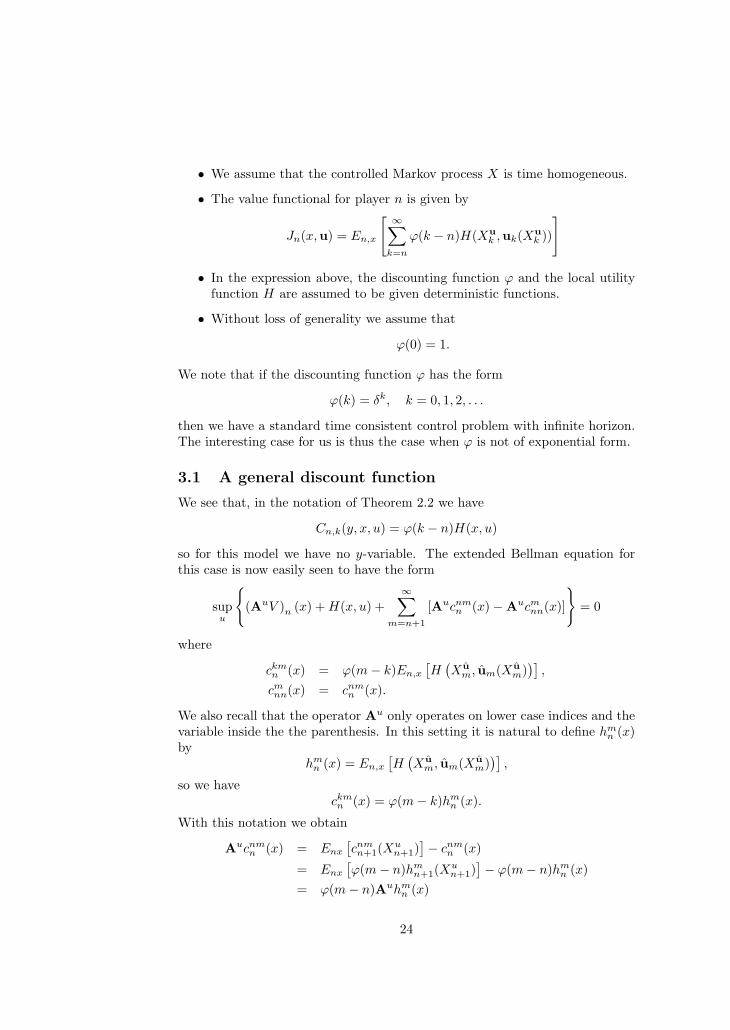
• We assume that the controlled Markov process X is time homogeneous.

• The value functional for player n is given by

Jn(x,u) = En,x

[ ∞∑k=n

ϕ(k − n)H(Xuk ,uk(Xu

k ))

]

• In the expression above, the discounting function ϕ and the local utilityfunction H are assumed to be given deterministic functions.

• Without loss of generality we assume that

ϕ(0) = 1.

We note that if the discounting function ϕ has the form

ϕ(k) = δk, k = 0, 1, 2, . . .

then we have a standard time consistent control problem with infinite horizon.The interesting case for us is thus the case when ϕ is not of exponential form.

3.1 A general discount function

We see that, in the notation of Theorem 2.2 we have

Cn,k(y, x, u) = ϕ(k − n)H(x, u)

so for this model we have no y-variable. The extended Bellman equation forthis case is now easily seen to have the form

supu

{(AuV )n (x) + H(x, u) +

∞∑m=n+1

[Aucnmn (x)−Aucm

nn(x)]

}= 0

where

ckmn (x) = ϕ(m− k)En,x

[H

(X u

m, um(X um)

)],

cmnn(x) = cnm

n (x).

We also recall that the operator Au only operates on lower case indices and thevariable inside the the parenthesis. In this setting it is natural to define hm

n (x)by

hmn (x) = En,x

[H

(X u

m, um(X um)

)],

so we haveckmn (x) = ϕ(m− k)hm

n (x).

With this notation we obtain

Aucnmn (x) = Enx

[cnmn+1(X

un+1)

]− cnm

n (x)

= Enx

[ϕ(m− n)hm

n+1(Xun+1)

]− ϕ(m− n)hm

n (x)= ϕ(m− n)Auhm

n (x)

24

and

Aucmnn(x) = Enx

[cn+1,mn+1 (Xu

n+1)]− cnm

n (x)

= Enx

[ϕ(m− n− 1)hm

n+1(Xun+1)

]− ϕ(m− n)hm

n (x)= ϕ(m− n− 1)Auhm

n (x)−∆ϕ(m− n)hmn (x),

where we have used the notation

∆ϕ(k) = ϕ(k)− ϕ(k − 1).

For the terms in the sum in the Bellman equation we thus have

Aucnmn (x)−Aucm

nn(x) = ∆ϕ(m− n)Auhmn (x) + ∆ϕ(m− n)hm

n (x)= ∆ϕ(m− n)Enx

[hm

n+1(Xun+1)

]= ∆ϕ(m− n)Puhm

n (x),

so the extended equation takes the form

supu

{(AuV )n (x) + H(x, u) +

∞∑m=n+1

∆ϕ(m− n)Puhmn (x)

}= 0

We may now use the fact that the setup is time homogeneous. Thus the valuefunction, will be time invariant and we have.

Jn(x,u) = J(x,u)

where

J(x,u) = Ex

[ ∞∑k=0

ϕ(k)H(Xuk ,uk(Xu

k )

]The equilibrium control, as well as the equilibrium value function, will also betime invariant so we have

un(x) = u(x),Vn(x) = V (x).

We also see that h will be time invariant in the sense that hmn (x) = hm−n

0 (x) sowe make the definition

hm(x) = hn+mn (x) = hm

0 (x),

and we note thath0(x) = H(x, u(x)).

Using the definition of hmkn (x) we also see that in fact

V (x) =∞∑

k=0

ϕ(k)hk(x).

25

The Bellman equation now takes the form

supu

{AuVn(x) + H(x, u) +

∞∑m=1

∆ϕ(m)Puhm(x)

}= 0

where, by definition,

Puhm(x) = Puhn+mn (x) = Enx

[hn+m

n+1 (Xun+1)

]= E0x

[hm−1

0 (Xu1 )

]= Ex

[hm−1(Xu

1 )]

We can thus state the final result.

Proposition 3.1 The extended Bellman system has the form

supu

{AuVn(x) + H(x, u) +

∞∑k=1

∆ϕ(k)Puhk(x)

}= 0

or, alternatively,

V (x) = supu

{H(x, u) + Ex [V (Xu

1 )] + Ex

[ ∞∑k=1

∆ϕ(k)hk−1(Xu1 )

]}.

In both cases, the function sequence hk(x) is determined by the recursion

hk+1 = Ex

[hk(X u

1 )],

h0(x) = H(x, u(x)).

3.2 Hyperbolic discounting

We now turn to the special case when ϕ is a “hyperbolic discounting function”.More precisely we assume that ϕ has the form

ϕ(0) = 1,

ϕ(k) = βδk, k = 1, 2, 3, . . .

where β ≥ 0 and 0 < δ < 1. In this case we have

∆ϕ(1) = βδ − 1,

∆ϕ(k) = βδk−1(δ − 1), k = 1, 2, . . .

Using the relation

V (x) =∞∑

k=0

ϕ(k)hk(x)

26

we obtain

Ex

[ ∞∑k=1

∆ϕ(k)hk−1(Xu1 )

]

= (βδ − 1)Ex

[h0(Xu

1 )]+ β(δ − 1)

∞∑k=2

δk−1Ex

[hk−1(Xu

1 )]

= (βδ − 1)Ex

[h0(Xu

1 )]+ (δ − 1)

∞∑k=1

βδkEx

[hk(Xu

1 )]

= (δ − 1)Ex

[h0(Xu

1 )]+ (δ − 1)

∞∑k=1

βδkEx

[hk(Xu

1 )]+ δ(β − 1)Ex

[h0(Xu

1 )]

= (δ − 1)Ex [V (Xu1 )] + δ(β − 1)Ex

[h0(Xu

1 )].

Plugging this into the recursive equation in Proposition 3.1 we thus have ourmain result for the hyperbolic discounting case.

Proposition 3.2 For the case of hyperbolic discounting, the extended Bellmansystem takes the form

V (x) = supu{δEx [V (Xu

1 )] + H(x, u) + δ(β − 1)Ex [H(Xu1 , u(Xu

1 ))]} .

Remark 3.1 We note that if β = 1 we have the standard exponential discount-ing ϕ(k) = δk and the extended Bellman equation in Proposition 3.2 trivializesto

V (x) = supu{δEx [V (Xu

1 )] + H(x, u)} .

which is the classical Bellman equation for the exponential discounting case.

4 Continuous time

We now turn to the more delicate case of continuous time models. We startby presenting the basic setup in term of a fairly general controlled Markovprocess. We then formulate the problem and formally define the continuous timeequilibrium concept. In order to derive the relevant extension of the Hamilton-Jacobi-Bellman equation we discretize, use our previously derived results indiscrete time, and go to the limit. Since the limiting procedure is somewhatinformal we need to prove a formal verification theorem, showing the connectionbetween the extended HJB equation and the previously defined equilibriumconcept.

4.1 Setup

We consider, on the time interval [0, T ] a controlled Markov process incontinous time. The process X lives on a measurable state space {X ,GX}, with

27

controls taking values in a measurable control space {U ,GU}. The way thatcontrols are influencing the dynamics of the process is formalized by specifyingthe controlled infinitesimal generator of X.

Definition 4.1 For any fixed u ∈ U we denote the corresponding infinitesimalgenerator by Au. For a control law u, the corresponding generator is denotedby Au.

As an example: of X is a controlled SDE of the form

dXt = µ(Xt, ut)dt + σ(Xt, ut)dWt,

then we have, for any real valued function f(t, x), and for any fixed u ∈ U

Auf(t, x) =∂f

∂t(t, x) + µ(x, u)

∂f

∂x(t, x) +

12σ2(t, x)

∂2f

∂x2(t, x)

For a control law u(t, x) we have

Auf(t, x) =∂f

∂t(t, x) + µ(x,u(t, x))

∂f

∂x(t, x) +

12σ2(x,u(t, x))

∂2f

∂x2(t, x).

By the Kolmogorov backward equation, the infinitesimal generator will, for anycontrol law u, determine the distribution of the process X, and to stress thisfact we will use the notation Xu

t . In particular we will have, for each h ∈ R anoperator Pu

h , operating on real valued functions of the form f(t, x), and definedas

Puhf(t, x) = E

[f(t + h, Xu

t+h)∣∣ Xt = x

]. (26)

We also recall thatAu =

dPuh

dh|h=0. (27)

4.2 Basic problem formulation

For a fixed (t, x) ∈ [0, T ]× X , a fixed control law u, we consider, as in discretetime, the simplified functional

J(t, x,u) = Et,x [F (x,XuT )] + G (x,Et,x [Xu

T ]) . (28)

The most general case will be treated in Section 4.3.2. As in discrete time wehave the game theoretic interpretation that, for each point t in time we havea player (“player t”) choosing ut who wants to maximize the functional above.Player t can, however, only affect the dynamics of the process X by choosing thecontrol ut exactly at time t. At another time, say s, the control us will be chosenby player s. We again attack this problem by looking for a Nash subgame perfectequilibrium point. The intuitive picture is exactly like in continuous time: Anequilibrium strategy u is characterized by the property that if all players on thehalf open interval (t, T ] uses u, then it is optimal for player t to use u.

28

However, in continuous time this is not a bona fide definition. Since playert can only choose the control ut exactly at time t, he only influences the controlon a time set of Lebesgue measure zero, and for most models this will haveno effect whatsoever on the dynamics of the process. We thus need anotherdefinition of the equilibrium concept, and we follow [4] and [5], who were thefirst to use the definition below.

Definition 4.2 Consider a control law u (informally viewed as a candidateequlibrium law). Choose a fixed u ∈ U , a fixed real number h > 0. Also fix anarbitrarily chosen initial point (t, x). Define the control law uh by

uh(s, y) ={

u, for t ≤ s < t + h, y ∈ Xu(s, y), for t + h ≤ s ≤ T, y ∈ X

If

lim infh→0

J(t, x, u)− J(t, x,uh)h

≥ 0,

for all u ∈ U , we say that u is an equilibrium control law. The equilibriumvalue function V is defined by

V (t, x) = J(t, x, u).

Remark 4.1 This is our continuous time formalization of the correspondingdiscrete time equilibrium concept. Note the necessity of dividing by h, since formost models we trivially would have

limh→0

{J(t, x, u)− J(t, x,uh)} = 0.

We also note that we do not get a perfect correspondence with the discrete timeequilibrium concept, since if the limit above equals zero for all u ∈ U , it is notclear that this corresponds to a maximum or just to a stationary point.

4.3 The extended HJB equation

We now assume that there exists an equilibrium control law u (not necessarilyunique) and we go on to derive and extension of the standard Hamilton-Jacobi-Bellman (henceforth HJB) equation for the determination of the correspondingvalue function V . To clarify the logical structure of the derivation we outlineour strategy as follows.

• We discretize (to some extent) the continuous time problem. We then useour results from discrete time theory to obtain a discretized recursion foru and we then let the time step tend to zero.

• In the limit we obtain our continuous time extension of the HJB equation.Not surprisingly it will in fact be a system of equations.

29

• In the discretizing and limiting procedure we mainly rely on informalheuristic reasoning. In particular we have do not claim that the derivationis a rigorous one. The derivation is, from a logical point of view, only ofmotivational value.

• We then go on to show that our (informally derived) extended HJB equa-tion is in fact the “correct” one, by proving a rigorous verification theorem.

4.3.1 Deriving the equation

In this section we will, in an informal and heuristic way, derive a continuoustime extension of the HJB equation. Note again that we have no claims to rigorin the derivation, which is only motivational. To this end we assume that thereexists an equilibrium law u and we argue as follows.

• Choose an arbitrary initial point (t, x). Also choose a “small” time incre-ment h > 0.

• Define the control law uh on the time interval [t, T ] by

uh(s, y) ={

u, for t ≤ s < t + h, y ∈ Xu(s, y), for t + h ≤ s ≤ T, y ∈ X

• If now h is “small enough” we expect to have

J(t, x,uh) ≤ J(t, x, u),

and in the limit as h → 0 we should have equality if u = u(t, x).

If we now use our discrete time results, with n and n+1 replaced by t and t+h,we obtain the inequality

(AuhV ) (t, x)−(Au

hf) (t, x, x)+(Auhfx) (t, x)−Au

h (G � g) (t, x)+(Huhg) (t, x) ≤ 0

where(Au

hV ) (t, x) = Et,x

[V (t + h, Xu

t+h)]− V (t, x)

and similarly for the other terms. We now divide the inequality by h and let htend to zero. The the operator Au

h will converge to the infinitesimal operatorAu, but the limit of h−1 (Hu

hg) (t, x) requires closer investigation.We have in fact

(Huhg) (t, x) = Gx(Et,x

[g(t + h, Xu

t+h)])−Gx(g(t, x)).

Furthermore we have the approximation

Et,x

[g(t + h, Xu

t+h)]

= g(t, x) + Aug(t, x) + o(h),

and using a standard Taylor approximation for Gx we obtain

Gx(Et,x

[g(t + h, Xu

t+h

]) = Gx(g(t, x)) + Gx

y(g(t, x)) ·Aug(t, x) + o(h),

30

whereGx

y(y) =∂Gx

∂y(y).

We thus obtain

limh→0

1h

(Huhg) (t, x) = Gx

y(g(t, x)) ·Aug(t, x).

Collecting all results we arrive at our proposed extension of the HJB equation.To stress the fact that the arguments above are largely informal we state theequation as a definition rather than as proposition.

Definition 4.3 The extended HJB system of equations for the Nash equilibriumproblem is defined as follows.

supu∈U

{(AuV ) (t, x)− (Auf) (t, x, x) + (Aufx) (t, x)

− Au (G � g) (t, x) + (Hug) (t, x)} = 0, 0 ≤ t ≤ T,

Aufy(t, x) = 0, 0 ≤ t ≤ T,

Aug(t, x) = 0, 0 ≤ t ≤ T,

V (T, x) = F (x, x) + G(x, x),fy(T, x) = F (y, x),g(T, x) = x.

Here u is the control law which realizes the supremum in the first equation, andfy, G � g, and Hg are defined by

fy(t, x) = f(t, x, y)(G � g) (t, x) = G(x, g(t, x)),

Hug(t, x) = Gy(x, g(t, x)) ·Aug(t, x),

Gy(x, y) =∂G

∂y(x, y).

We now have some comments on the extended HJB system.

• The first point to notice is that we have a system of recursion equation(5)-(10) for the simultaneous determination of V , f and g.

• In the case when F (x, y) does not depend upon x, and there is no G term,the problem trivializes to a standard time consistent problem. The terms(Auf) (t, x, x) + (Aufx) (t, x) in the V -equation cancel, and the systemreduces to the standard Bellman equation

(AuV ) (t, x) = 0,

V (T, x) = F (x).

31

• In order to solve the V -equation we need to know f and g but these aredetermined by the optimal control law u, which in turn is determined bythe sup-part of the V -equation.

• We can view the system as a fixed point problem, where the optimalcontrol law u solves an equation of the form M(u) = u. The mapping Mis defined by the following procedure.

– Start with a control u.

– Generate the functions f and g by the ODEs

Aufy(t, x) = 0,

Aug(t, x) = 0,

and the obvious terminal conditions.

– Now plug these choices of f and g into the V equation and solve itfor V . The control law which realizes the sup-part in the V -equationis denoted by M(u). The optimal control law is determined by thefixed point problem M(u) = u.

This fixed point property is rather expected since we are looking for aNash equilibrium point, and it is well known that such a point is typicallydetermined as fixed points of a mapping. We also note that we can viewthe system as a fixed point problem for f and g.

• The equations for g and fy state that the processes g(t, X ut ) and fy(t, X u

t ))are martingales. From the boundary conditions we then have the inter-pretation

f(t, x, y) = Et,x

[F (y, X u

T )],

g(t, x) = Et,x

[X u

T

].

• We note that the g function above appears, in a more restricted framework,already in [1], [4], and [5].

4.3.2 The general case

We now turn to the most general case of the present paper, where the functionalJ is given by

J(t, x,u) = Et,x

[∫ T

t

C (t, x, s, Xus ,u(Xu

s )) ds + F (t, x, XuT )

]+G (t, x, Et,x [Xu

T ]) .

(29)

32

Definition 4.4 Given the objective functional (29) the extended HJB equationfor V is given by

supu∈U

{(AuV ) (t, x) + C(t, x, t, x, u)−∫ T

t

(Aucs)(t, x, t, x)ds +∫ T

t

(Auctxs)(t, x)ds

− (Auf) (t, x, t, x) +(Auf tx

)(t, x)−Au (G � g) (t, x) + (Hug) (t, x)

}= 0,

with boundary condition

V (T, x) = F (T, x, x) + G(T, x, x).

Furthermore, the following hold.

1. For each fixed s and y, the function fsy(t, x) is defined by

Aufsy(t, x) = 0, 0 ≤ t ≤ T

fsy(T, x) = F (s, y, x)

2. The function g(t, x) is defined by

Aug(t, x) = 0, 0 ≤ t ≤ T

g(T, x) = x.

3. For each fixed s, r and y, the function csyr(t, x) is defined by

(Aucsyr)(t, x) = 0, 0 ≤ t ≤ r

csyr(r, x) = C(s, y, r, x, ur(x))

4. We have used the notation

f(t, x, s, y) = fsy(t, x)cs(t, x, t, x) = ctxs(t, x),

(G � g) (t, x) = G(t, x, g(t, x)),Hug(t, x) = Gy(t, x, g(t, x)) ·Aug(t, x),

Gy(x, y) =∂G

∂y(t, x, y).

5. The probabilistic interpretations of f , g, and c are given by

fsy(t, x) = Et,x

[F (s, y, X u

T )], 0 ≤ t ≤ T

g(t, x) = Et,x

[X u

T

], 0 ≤ t ≤ T

csyr(t, x) = Et,x

[C

(s, y, r, X u

r , u(X ur )

)], 0 ≤ t ≤ r.

6. In these expressions, u always denotes the equilibrium control law.

33

Remark 4.2 We can easily extend the result above to the case when the termG (t, x, Et,x [Xu

T ]) is replaced by

G (t, x, Et,x [h (XuT )])

for some function h. In this case we simply define g by

g(t, x) = Et,x

[h

(X u

T

)].

The extended HJB system then looks exactly as in Definition 4.4 above, apartfrom the fact that the boundary condition for g is changed to

g(T, x) = h(x).

See [8] for an interesting application.

Remark 4.3 It is of course also possible to include terms of the type

K(t, s, Etx [b(Xus )])

in the integral term of the value functional. The structure of the resulting HJBsystem is fairly obvious but we have omitted it since the present HJB system is,in our opinion, complicated enough as it is.

4.3.3 A simple special case

We see that the general extended HJB equation is quite complicated. In manyconcrete cases there are, however, cancellations between different terms in theequation. The simplest case occurs when the objective functional has the form

J(t, x,u) = Et,x [F (XuT )] + G (Et,x [Xu

T ]) ,

and X is a scalar diffusion of the form

dXt = µ(Xt, ut)dt + σ(Xt, ut)dWt.

In this case the extended HJB equation has the form

supu∈U

{AuV (t, x)−Au [G (g(t, x))] + G′(g(t, x))Aug(t, x)} = 0,

and a simple calculation shows that

−Au [G (g(t, x))] + G′(g(t, x))Aug(t, x) = −12σ2(x, u)G′′(g(t, x))g2

x(t, x),

where gx = ∂g∂x . Thus the extended HJB equation becomes

supu∈U

{AuV (t, x)− 1

2σ2(x, u)G′′(g(t, x))g2

x(t, x)}

= 0, (30)

We will use this result in Section 7 below.

34

4.3.4 A scaling result

We now extend the results from Section 2.4.5 to continuous time. Let us thusconsider the objective functional (29) above and denote, as usual, the equilib-rium control and value function by u and V respectively. Let ϕ : R → R be afixed real valued function and consider a new objective functional Jϕ, definedby,

Jϕ(t, x,u) = ϕ(x)J(t, x,u), n = 0, 1, . . . , T

and denote the corresponding equilibrium control and value function by uϕ andVϕ respectively. Since player No t is (loosely speaking) trying to maximizeJϕ(t, x,u) over ut, and ϕ(x) is just a scaling factor which is not affected by ut

the following result is intuitively obvious. The formal proof is, however, notquite trivial.

Proposition 4.1 With notation as above we have

Vϕ(t, x) = ϕ(x)V (t, x),uϕ(t, x) = u(t, x).

Proof. For notational simplicity we consider the case when J is of the form

J(t, x,u) = Et,x [F (x,XuT )] + G (x,Et,x [Xu

T ]) . (31)

The proof for the general case has exactly the same structure.For J as above we have the extended HJB system

supu∈U

{(AuV ) (t, x)− (Auf) (t, x, x) + (Aufx) (t, x)

− Au (G � g) (t, x) + Gy(x, g(t, x)) ·Aug(t, x)} = 0, 0 ≤ t ≤ T,

Aufy(t, x) = 0, 0 ≤ t ≤ T,

Aug(t, x) = 0, 0 ≤ t ≤ T,

V (T, x) = F (x, x) + G(x, x),fy(T, x) = F (y, x),g(T, x) = x.

We now recall the probabilistic interpretations

V (t, x) = Et,x

[F (x,X u

T )]+ G

(x,Et,x

[X u

T

])f(t, x, y) = Et,x

[F (y, X u

T )],

g(t, x) = Et,x

[X u

T

].

and the definition(G � g) (t, x) = G(x, g(t, x)).

From this it follows that

V (t, x) = f(t, x, x) + (G � g) (t, x),

35

so the first HJB equation above can be written

supu∈U

{(Aufx) (t, x) + Gy(x, g(t, x)) ·Aug(t, x)} = 0.

We now turn to Jϕ, which can be written

J(t, x,u) = Et,x [Fϕ(x,XuT )] + Gϕ (x,Et,x [Xu

T ]) ,

where

Fϕ(x, y) = ϕ(x)F (x, y),Gϕ(x, y) = ϕ(x)G(x, y),

and we note that∂Gϕ

∂y(x, y) = ϕ(x)Gy(x, y)

We thus obtain the HJB equation

supu∈U

{(Aufx

ϕ

)(t, x) + ϕ(x)Gy(x, gϕ(t, x)) ·Augϕ(t, x)

}= 0,

with fϕ and gϕ defined by

Auϕfyϕ(t, x) = 0,

Auϕgϕ(t, x) = 0,

fyϕ(T, x) = ϕ(y)F (y, x),

gϕ(T, x) = x.

From this it follows that we can write

fϕ(t, x, y) = ϕ(y)f0(t, x, y),gϕ(t, x) = g0(t, x)

where

Auϕfy0 (t, x) = 0,

Auϕg0(t, x) = 0,

fy0 (T, x) = F (y, x),

g0(T, x) = x.

and the HJB equation has the form

supu∈U

{ϕ(x) (Aufx0 ) (t, x) + ϕ(x)Gy(x, g0(t, x)) ·Aug0(t, x)} = 0,

or, equivalently,

supu∈U

{(Aufx0 ) (t, x) + Gy(x, g0(t, x)) ·Aug0(t, x)} = 0.

36

We thus see that the system for f , g, and u is exactly the same as that for f0,g0, and uϕ. We thus have

fϕ(t, x, y) = ϕ(y)f(t, x, y),gϕ(t, x) = g(t, x),

uϕ = u.

Moreover, sinceVϕ(t, x) = fϕ(t, x, x) + (Gϕ � gϕ) (t, x),

we obtainVϕ(t, x) = ϕ(x)V (t, x).

4.3.5 A Verification Theorem

As we have noted above, the derivation of the continuous time extension of theHJB equation is rather informal. It seems reasonable to expect that the systemin Definition 4.3 will indeed determine the equilibrium value function V , but sofar nothing has been formally proved. However, the following two conjecturesare natural.

• Assume that there exists an equilibrium law u and that V is the corre-sponding value function. Assume furthermore that V is regular enoughto allow allow Au to operate on it (in the diffusion case this would implyV ∈ C1,2). Define f and g by

f(t, x, y) = Et,x

[F (y, X u

T )], (32)

g(t, x) = Et,x

[X u

T

]. (33)

Then V satisfies the extended HJB system and u realizes the supremumin the equation.

• Assume that V , f , and g solves the extended HJB system and that thesupremum i the V -equation is attained for every (t, x). Then there existsan equlibrium law u, and it is given by the optimal u in the in the V -equation. Furthermore, V is the corresponding equilibrium value function,and f and g allow for the interpretations (32)-(33).

In this paper we do not attempt to prove the first conjecture. Even for astandard time consistent control problem, it is well known that this is technicallyquite complicated, and it typically requires the theory of viscosity solutions. Wewill, however, prove the second conjecture. This obviously has the form of averification result, and from standard theory we would expect that it can beproved with a minimum of technical complexity.

37

Theorem 4.1 (Verification Theorem) Assume that V , f , g is a solutionof the extended system in Definition 4.3, and that the control law u realizesthe supremum in the equation. Then u is an equilibrium law, and V is thecorresponding value function. Furthermore, f and g can be interpreted accordingto (32)-(33).

Proof. The proof consists of two steps:

• We start by showing that V is the value function corresponding to u,i.e. that V (t, x) = J(t, x, u), and that f and g have the interpretations(32)-(33).

• In the second step we then prove that u is indeed an equilibrium controllaw.

To show that V (t, x) = J(t, x, u), we use the V equation to obtain:(AuV

)(t, x)−

(Auf

)(t, x, x) +

(Aufx

)(t, x)

−Au (G � g) (t, x) +(Hug

)(t, x) = 0,

whereHug(t, x) = Gy(x, g(t, x)) ·Aug(t, x).

Since V , f , and g satsifies the extended HJB, we also have(Aufx

)(t, x) = 0, (34)

Aug(t, x) = 0, (35)

and we thus have the equation(AuV

)(t, x)−

(Auf

)(t, x, x)−Au (G � g) (t, x) = 0. (36)

We now use Dynkin’s Theorem which says that if X is a process with infinites-imal operator A, and if h(t, x) is a sufficiently integrable real valued function,then the process

h(t, Xt)−∫ t

0

Ah(s,Xs)ds

is a martingale. Using Dynkin’s Theorem we thus have

Et,x [V (T,XT )] = V (t, x) + Et,x

[∫ T

t

AuV (s,X us )ds

],

and from (36) we obtain

Et,x

[V (T,X u

T )]

= V (t, x)+Et,x

[∫ T

t

Auf(s,X us , X u

s ds)

]+Et,x

[∫ T

t

Au (G � g) (s,X us )ds

]

38

We again refer to Dynkin and obtain

Et,x

[∫ T

t

Auf(s,X us , X u

s )ds

]= Et,x

[f(T,X u

T , X uT )

]− f(t, x, x),

Et,x

[∫ T

t

Au (G � g) (s,X us )ds

]= Et,x

[G(XT , g(T,X u

T ))]−G(x, g(t, x)).

Using this and the boundary conditions for f and g we get

Et,x

[F (X u

T , X uT ) + G(X u

T , X uT )

]= V (t, x) + Et,x

[F (X u

T , X uT )

]− f(t, x, x)

+ Et,x

[G(X u

T , X uT )

]−G(x, g(t, x)),

i.e.V (t, x) = f(t, x, x) + G(x, g(t, x)). (37)

Now, from (34)-(35) it follows that the processes fy(s,X us ) and g(s,X u

s ) aremartingales, so from the boundary conditions for f and g we obtain

f(t, x, y) = Et,x

[F (y, X u

T )],

g(t, x) = Et,x

[X u

T

].

This shows that f and g have the correct interpretation and, plugging it into(37) we obtain

V (t, x) = Et,x

[F (x,X u

T )]+ G(x,Et,x

[X u

T

])) = J(t, x, u).

We now go on to show that u is indeed an equilibrium law. To that endwe construct, for any h > 0 and an arbitrary u ∈ U , the control law uh definedin Definition 4.2. From Lemma 2.2, applied to the points t and t + h, we have

Jn(x,u) = Et,x

[J(t + h, Xu

t+h,u)]

−{Et,x

[fu(t + h, Xu

t+h, Xut+h)

]− Et,x

[fu(t + h, Xu

t+h, x)]}

−{Et,x

[G

(Xu

t+h, gu(t + h, Xut+h)

)]−G

(x,Et,x

[gu(t + h, Xu

t+h)])}

.

where, for ease of notation, we have suppressed the lower index h of uh. By theconstruction of u we have

J(t + h, Xut+h,u) = V (t + h, Xu

t+h),fu(t + h, Xu

t+h, x) = f(t + h, Xut+h, x),

gu(t + h, Xut+h) = g(t + h, Xu

t+h),

so we obtain

Jn(x,u) = Et,x

[V (t + h, Xu

t+h)]

−{Et,x

[f(t + h, Xu

t+h, Xut+h)

]− Et,x

[f(t + h, Xu

t+h, x)]}

−{Et,x

[G

(Xu

t+h, g(t + h, Xut+h)

)]−G

(x,Et,x

[g(t + h, Xu

t+h)])}

.

39

Furthermore, from the V -equation we have

(AuV ) (t, x)− (Auf) (t, x, x) + (Aufx) (t, x)−Au (G � g) (t, x) + (Hug) (t, x) ≤ 0,

for all u ∈ U . Discretizing this gives us

Et,x

[V (t + h, Xu

t+h)]− V (t, x)−

{Et,x

[f(t, Xu

t+h, Xut+h)

]− f(t, x, x)

}+Et,x

[f(t, Xu

t+h, x)]− f(t, x, x)

−Et,x

[G(t + h, g(t + h, Xu

t+h)]+ G(x, g(t, x))

+G(x,Et,x

[g(t + h, Xu

t+h)]−G(x, g(t, x)) ≤ o(h),

or, after simplification,

V (t, x) ≥ Et,x

[V (t + h, Xu

t+h)]− Et,x

[f(t, Xu

t+h, Xut+h)

]+ Et,x

[f(t, Xu

t+h, x)]

− Et,x

[G(t + h, g(t + h, Xu

t+h)]+ G(x,Et,x

[g(t + h, Xu

t+h)]+ o(h).

Using the expression for Jn(x,u) above, and the fact that V (t, x) = J(t, x, u),we obtain

J(t, x, u)− J(t, x,u) ≥ o(h),

so

lim infh→0

J(t, x, u)− J(t, x,u)h

≥ 0,

and we are done.

5 An equivalent time consistent problem

The object of the present section is to provide a surprising link between timeinconsistent and time consistent problems. To this end we go back to the generalcontinuous time extended HJB equation. The first part of this reads as

supu∈U

{(AuV ) (t, x) + C(x, x, u)−∫ T

t

(Aucs)t(x, x)ds +∫ T

t

(Aucs,x)t(x)ds

− (Auf) (t, x, x) + (Aufx) (t, x)−Au (G � g) (t, x) + (Hug) (t, x)} = 0.

Let us now assume that there exists an equilibrium control law u. Using u wecan then construct c, f and g by solving the associated equations in Definition4.3. We now define the function h by

h(t, x, u) = C(x, x, u)−∫ T

t

(Aucs)t(x, x)ds +∫ T

t

(Aucs,x)t(x)ds

− (Auf) (t, x, x) + (Aufx) (t, x)−Au (G � g) (t, x) + (Hug) (t, x).

40

With this definition of h, the equation for V above and its boundary conditionbecome

supu∈U

{(AuV ) (t, x) + h(t, x, u)} = 0,

V (T, x) = F (x, x) + G(x, x).

We now observe, by inspection, that this is a standard HJB equation for thestandard time consistent optimal control problem to maximize

Et,x

[∫ T

t

h(s,Xs, us)ds + F (XT , XT ) + G(XT , XT )

]. (38)

We have thus proved the following result.

Proposition 5.1 For every time inconsistent problem in the present frame-work there exists a standard, time consistent optimal control problem with thefollowing properties.

• The optimal value function for the standard problem coincides with theequilibrium value function for the time inconsistent problem.

• The optimal control for the standard problem coincides with the equilibriumcontrol for the time inconsistent problem.

• The objective functional for the standard problem is given by (38).

We immediately remark that the Proposition above is mostly of theoreticalinterest, and of little “practical” value. The reason is of course that in orderto formulate the equivalent standard problem we need to know the equilibriumcontrol u. In our opinion it is, however, quite surprising.

Furthermore, Proposition 5.1 has modeling consequences for economics.Suppose that you want to model consumer behavior. You have done this usingstandard time consistent dynamic utility maximization and now you are con-templating to introduce time inconsistent preferences to obtain a richer class ofconsumer behavior. Proposition 5.1 then tells us that from the point of viewof revealed preferences, nothing is gained by introducing time inconsistent pref-erences: Every kind of behavior that can be generated by time inconsistencycan also be generated by time consistent preferences. We immediately remark,however, that even if a concrete model of time inconsistent preferences is, insome sense, “natural”, the corresponding time consistent preferences may lookextremely “weird”.

6 Example: Non exponential discounting

We now illustrate the theory developed above, and the first example we consideris a fairly general case of a control problem with non exponential discounting.The model is specified as follows.

41

• We consider a controlled, not necessarily time homogeneous, Markov pro-cess in continuous time with controlled infinitesimal generator Au.

• The value functional for player number t is given by

J(t, c,u) = Etx

[∫ T

t

ϕ(t− s)H(Xus , u (Xu

s ))ds + ϕ(T − t)Γ (XuT )

],

where the discounting function ϕ(t), the local utility function H(x, u) andthe final state utility function Γ(x) are deterministic functions.

• Without loss of generality we assume that

ϕ(0) = 1.

In the notation of Definition 4.4 we see that we have no G-term so the extendedHJB equation has the form

supu∈U

{(AuV ) (t, x) + C(t, x, t, x, u)−∫ T

t

(Aucs)(t, x, t, x)ds +∫ T

t

(Auctxs)(t, x)ds

− (Auf) (t, x, t, x) +(Auf tx

)(t, x)

}= 0,

We recall the relations

fsy(t, x) = Et,x

[F (s, y, X u

T )], 0 ≤ t ≤ T

f(t, x, t, x) = f tx(t, x),crys(t, x) = Et,x

[C

(r, y, s, X u

s , u(X us )

)], 0 ≤ t ≤ r.

cs(t, x, t, x) = csxt(t, x)

as well as the notational convention that the operator Au operates only onthe variables within the parenthesis, whereas upper case indices are treated asconstant parameters. In our case the y variable is not present, so we can write

fsy(t, x) = fs(t, x)crys(t, x) = crs(t, x)

and the extended HJB equation takes the form

supu∈U

{(AuV ) (t, x) + C(t, t, x, u)−∫ T

t

(Aucs)(t, t, x)ds +∫ T

t

(Aucts)(t, x)ds

− (Auf) (t, t, x) +(Auf t

)(t, x)

}= 0,

where

fs(t, x) = Et,x

[F (s,X u

T )], 0 ≤ t ≤ T,

f(t, t, x) = f t(t, x),crs(t, x) = Et,x

[C

(r, s,X u

s , u(X us )

)],

cs(t, t, x) = cts(t, x).

42

In our case we furthermore have

C(t, s, x, u) = ϕ(s− t)H(x, u),F (t, x) = ϕ(T − t)Γ(x).

so we can write

fs(t, x) = ϕ(T − s)γ(t, x),crs(t, x) = ϕ(s− r)hs(t, x),

cs(t, t, x) = ϕ(s− t)hs(t, x)

where γ and h are defined by

γ(t, x) = Et,x

[Γ(X u

T )], 0 ≤ t ≤ T,

hs(t, x) = Et,x

[H

(X u

s , u(X us )

)], 0 ≤ t ≤ s.

We now easily obtain

C(t, t, x, u) = H(x, u),Aucrs(t, x) = ϕ(s− r)Auhs(t, x),

Aucs(t, t, x) = ϕ(s− t)Auhs(t, x)− ϕ′(t− s)hs(t, x),Auf t(t, x) = ϕ(T − t)Auγs(t, x),

Auf(t, t, x) = ϕ(T − t)Auγ(t, x)− ϕ′(T − t)γ(t, x).

We have thus proved the following result.

Proposition 6.1 The extended HJB system has the form

supu∈U

{AuV (t, x) + H(x, u) +

∫ T

t

ϕ′(s− t)hs(t, x)ds + ϕ′(T − t)γ(t, x)

}= 0,

V (T, x) = Γ(x),

where hs and γ are determined by

Auhs(t, x) = 0, 0 ≤ t ≤ s,

Auγ(t, x) = 0, 0 ≤ t ≤ T,

hs(s, x) = H (x, us(x)) ,

γ(T, x) = Γ(x).

This generalizes the corresponding results in [4] and [5], where special cases aretreated in great detail.

43

7 Example: Mean-variance control

In this example we will consider dynamic mean variance optimization. This isa continuous time version of a standard Markowitz investment problem, wherewe penalize the risk undertaken by the conditional variance. As noted in theintroduction, in a Wiener driven framework this example is studied intensivelyin [1], where the authors also consider the case of multiple assets, as well as thecase of a hidden Markov process (unobservable factors) driving the parametersof the asset price dynamics. For illustrative purposes we first consider thesimplest possible case of a Wiener driven single risky asset and, without anyclaim of originality, re-derivethe corresponding results of [1]. We then extendthe model in [1] and study the case when the risky asset is driven by a pointprocess as well as by a Wiener process.

7.1 The simplest case

We consider a market formed by a risky asset with price process S and a riskfree money account with price process B. The price dynamics are given by

dSt = αStdt + σStdWt,

dBt = rBtdt,

where α and σ are known constants, and r is the constant short rate.Let ut be the amount of money invested in the risky asset at time t. The

value Xt of a self-financing portfolio based on S and B will then evolve accordingto the SDE

dXt = [rXt + (α− r)ut]dt + σutdWt. (39)

Our value functional is given by

J(t, x,u) = Et,x [XuT ]− γ

2V art,x (Xu

T ) ,

so we want to maximize expected return with a penalty term for risk. Remem-bering the definition for the conditional variance

V art,x[XT ] = Et,x[X2T ]− E2

t,x[XT ],

we can re-write our objective functional as

J(t, x,u) = Et,x [F (XuT )]−G(Et,x [Xu

T ])

where F (x) = x − γ2 x2 and G(x) = γ

2 x2. As seen in the previous sections, theterm G(Et,x [XT ]) leads to a time inconsistent game theoretic problem.

The extended HJB equation is then given by the following PDE system:

supu

{[rx + (α− r)u]Vx +

12σ2u2Vxx −Au(G ◦ g) + Hug

}= 0,

V (T, x) = x,

Aug = 0,

g(T, x) = x,

44

where lower case index denotes the corresponding partial derivative. This caseis covered in Section 4.3.3, and from (30) we can simplify to

Vt + supu

{[rx + (α− r)u]Vx +

12σ2u2Vxx −

γ

2σ2u2g2

x

}= 0

V (T, x) = x

Aug = 0g(T, x) = x

Given the linear structure of the dynamics, as well as of the boundaryconditions, it is natural to make the Ansatz

V (t, x) = A(t)x + B(t)g(t, x) = a(t)x + b(t).

With this trial solution the HJB equation becomes

Atx + Bt + supu

{[rx + (α− r)u]A− γ

2σ2u2a2

}= 0, (40)

atx + bt + [rx + (α− r)u]a = 0, (41)A(T ) = 1,

B(T ) = 0,

a(T ) = 1,

b(T ) = 0.

We first solve the static problem embedded in (40). From the first order condi-tion, we obtain the optimal control as

u(t, x) =1γ

α− r

σ2

A(t)a2(t)

,

so the optimal control does not depend on x. Substituting this expression for uinto (40) we obtain:

Atx + Bt + Arx +12γ

(α− r)2

σ2

A2

a2= 0.

By separation of variables we then get the following system of ODEs.

At + Ar = 0,

A(T ) = 1,

Bt +12γ

(α− r)2

σ2

A2

a2= 0,

B(T ) = 0.

We immediately obtainA(t) = er(T−t).

45

Inserting this expression for A into the second ODE yields

Bt +12γ

(α− r)2

σ2

e2r(T−t)

a2= 0, (42)

B(T ) = 0.

This equation contain the unknown function a, and to determine this we useequation (41). Inserting the expression for u into (41) gives us

atx + bt + rxa +1γ

(α− r)2

σ2

er(T−t)

a= 0,

a(T ) = 1,

b(T ) = 0.

Again we have separation of variables and obtain the system

at + ar = 0,

bt +1γ

(α− r)2

σ2

er(T−t)

a= 0.

This yieldsa(t) = er(T−t),

and the ODE for b then takes the form

bt =1γ

(α− r)2

σ2,

b(T ) = 0.

We thus have

b(t) =1γ

(α− r)2

σ2(T − t).

Introducing the results in the optimal control formula, we get

u(t, x) =1γ

α− r

σ2e−r(T−t).

Using the expression for a above, we can go back to equation (42) which nowtakes the form

Bt +12γ

(α− r)2

σ2= 0,

so

B(t) =12γ

(α− r)2

σ2(T − t).

Thus, the optimal value function is given by

V (t, x) = er(T−t)x +12γ

(α− r)2

σ2(T − t)

We summarize the results as follows:

46

Proposition 7.1 For the model above we have the following results.

• The optimal amount of money invested in a stock is given by

u(t, x) =1γ

α− r

σ2e−r(T−t).

• The equilibrium value function is given by

V (t, x) = er(T−t)x +12γ

(α− r)2

σ2(T − t).

• The expected value of the optimal portfolio is given by

Et,x [XT ] = er(T−t)x +1γ

(α− r)2

σ2(T − t).

Using Proposition 5.1 we can also construct the equivalent standard timeconsistent optimization problem. An easy calculation gives us the followingresult.

Proposition 7.2 The equivalent (in the sense of Proposition 5.1) time consis-tent problem is to maximize the functional

maxu

Et,x

[XT − γσ2

2

∫ T

t

e2r(T−s)u2sds

]

given the dynamics (39).

We note in passing thatσ2u2

t dt = d〈X〉t.

7.2 A point process extension

We will now present an extension of the mean variance problem when the stockdynamics are driven by a jump diffusion. We consider a single risky asset withprice S and a bank account with price process B. The results below can beeasily extended to the case of multiple assets, but for ease of exposition, werestrict ourselves to the scalar case. The dynamics are given by

dSt = α(t, St)Stdt + σ(t, St)StdWt + St−

∫Z

β(z)µ(dz, dt),

dBt = rdt.

Here W is a scalar Wiener process and µ is a marked point process on themark space Z with deterministic intensity measure λ(dz). Furthermore, α(t, s),σ(t, s) and β(z) are known deterministic functions and r is a known constant.

47

As before ut denotes the amount of money invested in the stock at time t,and X is the value process for a self financing portfolio based on S and B. Thedynamics of Xt are then given by

dXt = [rXt + (α(t, St, Yt)− r)u]dt + σ(t, St, Yt)udWt + ut−

∫Z

β(z)µ(dz, dt).

Again we study the case of mean-variance utility, i.e.

J(t, x,u) = Et,x [XuT ]− γ

2V art,x (Xu

T ) .

The extended HJB system now has the form

supu{AuV (t, x, s)−Au(G ◦ g)(t, x, s) + (Hug) (t, x, s)} = 0, (43)

V (T, x, s) = x,

Aug = 0, (44)g(T, x, s) = x.

As before, we make the Ansatz

V (t, x, s) = A(t)x + B(t, s),g(t, x, s) = a(t)x + b(t, s),

A(T ) = 1,

B(T, s) = 0a(T ) = 1,

b(T, s) = 0.

After some simple but tedious calculations, equation (43) can be re-written as

supu{Atx + Bt + A [rx + (α− r)u] + αsBs +

12σ2s2Bss + Au

∫Z

β(z)λ(dz)

+∫

Z

[B(t, s(1 + β(z)))−B(t, s)︸ ︷︷ ︸∆βB(t,s,z)

]λ(dz)− 12σ2γ[au + bss]2

−γ

2

∫Z

[auβ(z) + b(t, s(1 + β(z)))− b(t, s)︸ ︷︷ ︸∆βb(t,s,z)

]2λ(dz)} = 0 (45)

First, we solve the embedded static problem in (45)

maxu

{(α− r)Au + Au

∫Z

β(z)λ(dz)− 12σ2[au + bss]2 −

γ

2

∫Z

[auβ(z) + ∆βb]λ(dz)}

and obtain the optimal control

u(t, x, s) =

[α(t, s)− r +

∫Z

β(z)λ(dz)]A(t)

γa2(t)[σ2(t, s) +∫

Zβ2(z)λ(dz)]

−σ(t, s)bs(t, s)s +

∫Z

β(z)∆βb(t, s, z)λ(dz)a(t)[σ2(t, s) +

∫Z

β2(z)λ(dz)]

48

Again we see that the optimal control does not depend on x. We can plug theoptimal control into equation (45) and as before, we can separate variables toobtain an ODE for A(t) and a PIDE for B(t, s). The ODE for A is

At + rA = 0A(T ) = 0

with solution A(t) = er(T−t). The PIDE for B(t, s) becomes

Bt + (α− r)u + αsBs +12σ2s2Bss + Au

∫Z

β(z)λ(dz) (46)

+∫

Z

[∆βB]λ(dz)− 12σ2γ[a(t)u + bss]2 (47)

−γ

2

∫Z

[a(t)uβ(z) + ∆βb]2λ(dz) = 0 (48)

B(T, s) = 0 (49)

In order to solve this we need to determine the functions a(t) and b(t, s). Tothis end we use (44). This can be rewritten as

atx + bt + [rx + (α− r)u]a + αsbs +12σ2s2bss

+au

∫Z

β(z)λ(dz) +∫

Z

∆βbλ(dz) = 0. (50)

with the appropriate boundary conditions for a and b. By separation of variableswe obtain the ODE

at + ra = 0,

a(T ) = 1,

and the PIDE

bt + (α− r)ua + αsbs +12σ2s2bss + au

∫Z

β(z)λ(dz) +∫

Z

∆βbλ(dz) = 0,

b(T, s) = 0.

From the ODE we have a(t) = er(T−t) and, plugging this expression intothe previous formula for u, gives us

u =α− r +

∫Z

β(z)λ(dz)γ[σ2 +

∫Z

β2(z)λ(dz)]e−r(T−t) −

σbss +∫

Zβ(z)∆βbλ(dz)

[σ2 +∫

Zβ2(z)λ(dz)]

e−r(T−t)

We can now insert this expression, as well as the formula for a, into thePIDE for b above to obtain the PIDE

49

bt +

[α−

[α− r +

∫Z

β(y)λ(dy)]σ2

[σ2 +∫

Zβ2(y)λ(dy)]

]sbs +

12σ2s2bss +

[α− r +

∫Z

β(y)λ(dy)]2

γ[σ2 +∫

Zβ2(y)λ(dy)]∫

Z

∆βb(t, s, z){

1−α− r +

∫Z

β(y)λ(dy)[σ2 +

∫Z

β2(y)λ(dy)]β(z)

}λ(dz) = 0

b(T, s) = 0

This rather forbidding looking equation cannot in general be solved explicitly,but by applying a Feynman-Kac representation theorem we can represent thesolution as

b(t, s) = EQt,s

[∫ T

t

[α(τ, Sτ )− r +

∫Z

β(z)λ(dz)]2

γ[σ2(τ, Sτ ) +∫

Zβ2(z)λ(dz)]

dτ

]. (51)

Here the measure Q is absolutely continuous w.r.t. P , and the likelihood process

Lt =dQ

dPon Ft,

has dynamics given by

dLt = LtϕdWt + Lt−

∫Z

η(z) [µ(dz, dt)− λ(dz)dt] ,

with ϕ and η given by

ϕ(t, s) = −[α(t, s)− r +

∫Z

β(y)λ(dy)]σ(t, s)

[σ2(t, s) +∫

Zβ2(y)λ(dy)]

,

η(t, s, z) = −[α(t, s)− r +

∫Z

β(y)λ(dy)]

[σ2(t, s) +∫

Zβ2(y)λ(dy)]

β(z).

From the Girsanov Theorem it follows that the Q intensity λQ, of the pointprocess µ(dt, dz) is given by

λQ(t, s, dz) =

{1−

[α(t, s)− r +

∫Z

β(y)λ(dy)]

[σ2(t, s) +∫

Zβ2(y)λ(dy)]

β(z)

}λ(dz),

and that

dWt = −[α(t, St)− r +

∫Z

β(y)λ(dy)]σ(t, St)

[σ2(t, St) +∫

Zβ2(y)λ(dy)]

dt + dWQt

where WQ is Q a Wiener process. A simple calculation now shows that the Qdynamics of the stock prices S are given by

dSt = rStdt + Stσ(t, St)dWQt + St−

∫Z

β(z)[µ(dt, dz)− λQ(t, St, dz)

]50

so the measure Q is in fact a risk neutral martingale measure, and it is easy tocheck (see for example [2]) that Q is in fact the so called “minimal martingalemeasure” used in the context of local risk minimization and developed in [11]and related papers. This fact was, in a Wiener process framework, observedalready in [1].

Performing similar calculations, one can show that the solution of the PIDE(48)-(49) can be represented as

B(t, s) = EQt,s

[∫ T

t

(α− r +∫

Zβ(z)λ(dz))2

γ[σ2 +∫

Zβ2(z)λ(dz)]

dτ

]

−EQt,s

[∫ T

t

12σ2γ[er(T−τ)u + bss]2dτ

]

−EQt,s

[∫ T

t

γ

2

∫Z

[er(T−τ)uβ(z) + ∆βb]2λ(dz)dτ

], (52)

with Q as above.We can finally summarize our results.

Proposition 7.3 With notation as above, the following hold.

• The optimal amount of money invested in a stock is given by

u =(α− r +

∫Z

β(z)λ(dz))γ[σ2 +

∫Z

β2(z)λ(dz)]e−r(T−t)−

(σbss +∫

Zβ(z)∆βb(z)λ(dz))

[σ2 +∫

Zβ2(z)λ(dz)]

e−r(T−t)

• The mean-variance utility of the optimal portfolio is given by

U(t, x) = er(T−t)x + b(t, s)

where b(t, s) is given by stochastic representation (51).

• The expected terminal value of the optimal portfolio is

Et,x [XT ] = xer(T−t) + B(t, s)

where x is the present portfolio value and B(t, s) is given by the stochasticrepresentation (52).

8 Example: The time inconsistent linear quadraticregulator

In this example we consider a problem where the utility function at T dependson the current state Xt. The model is specified as follows.

51

• The value functional for player t is given by

Etx

[12

∫ T

t

u2sds

]+

γ

2Etx

[(XT − x)2

]where γ is a positive constant.

• The state process X is scalar with dynamics

dXt = [aXt + but] dt + σdWt,

where a, b and σ are given constants.

• The control u is scalar with no constraints.

This is a time inconsistent version of the classical linear quadratic regulator.Loosely speaking we want control the system so that the final sate XT is closeto x while at the same time keeping the control energy (formalized by theintegral term) is small. The time inconsistency stems from the fact that thetarget point x = Xt is changing as time goes by.

For this problem we have

F (x, y) = y − x,

C(u) =12u2

and as usual we introduce the functions fy(t, x) and f(t, x, x) by

fy(t, x) = Etx

[(X u

T − y)2

],

f(t, x, y) = fy(t, x).

The extended HJB system takes the form

infu

{AuV (t, x) +

12u2 + Aufx(t, x)−Auf(t, x, x)

}= 0, 0 ≤ t ≤ T

V (T, x) = 0,

Aufy(t, x) = 0, 0 ≤ t ≤ T

fy(T, x) =γ

2(x− y)2.

From the X dynamics we see that

Au =∂

∂t+ (ax + bu)

∂

∂x+

12σ2 ∂2

∂x2,

so we obtain

Aufy(t, x) =∂fy

∂t(t, x) + (ax + bu)

∂fy

∂x(t, x) +

12σ2 ∂2fy

∂x2(t, x)

Auf(t, x, x) =∂f

∂t+ (ax + bu)

[∂f

∂x+

∂f

∂y

]+

12σ2

[∂2f

∂x2+

∂2f

∂y2+

∂2f

∂x∂y

],

52

where the derivatives of f in the last equation are evaluated at (t, x, x). We thusobtain the following form of the HJB equation, where for shortness of notationwe denote partial derivatives by lower case index so, for example, fx = ∂f

∂x . AllV terms are evaluated at (t, x) and all f terms are evaluated at (t, x, x).

infu

{Vt + (ax + bu)Vx +

12σ2Vxx +

12u2 − (ax + bu)fy − σ2fxy − σ2fyy

}= 0,

V (T, x) = 0.

The coupled system for fy is given by

fyt (t, x) + [ax + bu(t, x)] fy

x (t, x) +12σ2fy

xx(t, x) = 0, 0 ≤ t ≤ T,

fy(T, x) =γ

2(x− y)2.

The first order condition in the HJB equation gives us

u(t, x) = b {fy(t, x, x)− Vx(t, x)}

and, inspired of the standard regulator problem, we now make the Ansatz (at-tempted solution)

f(t, x, y) = A(t)x2 + B(t)y2 + C(t)xy + D(t)x + F (t)y + H(t), (53)V (t, x) = α(t)x2 + β(t)x + ε(t), (54)

where all coefficients are deterministic functions of time. We now insert theAnsatz into the HJB system, and perform an extremely large number of ex-tremely boring calculations. As a result of these calculations, it turns out thatthe variables separate in the expected way and we have the following result.

Proposition 8.1 For the time inconsistent regulator, we have the structure(53)-(54), where the coefficient functions solve the following system of ODEs.

At + 2aA + 2b2A (2B + C − 2α) = 0,

Bt = 0,

Ct + aC = 0,

Dt + aD + b2D (2B + C − 2α) + 2b2A(F − β) = 0,

Ft + b2CF − βb2C = 0,

Ht + b2(F − β)D + σ2A = 0,

αt + 2aα + 2αb2 (2B − C − 2α) +12b2 (2B + C − 2α)2 − a (2B + C)

−b2 (2B + C) (2B + C − 2α) = 0,

βt + αβ + βb2 (2B + C − 2α) + 2αb2 (F − β) + b2 (2B + C − 2α) (F − β)−aF − b2F (2B + C − 2α)− b2 (F − β) (2B + C) = 0,

εt + b2β (F − β) + σ2a +12b2 (F − β)2 − b2 (F − β) F − σ2C − σ2B = 0.

53

With boundary conditions

A(T ) =γ

2, B(T ) =

γ

2, C(T ) = −γ,

D(T ) = 0, F (T ) = 0, H(T ) = 0,

α(T ) = 0, β(T ) = 0, ε(T ) = 0.

9 Conclusion and future research

In this paper we have presented a fairly general class of time inconsistent stochas-tic control problems. Using a game theoretic perspective we have, in discrete aswell as in continuous time, derived a system of equations for the determinationof the subgame perfect Nash equilibrium control, as well as for the correspondingequilibrium value function. The system is an extension of the standard dynamicprogramming equation for time consistent problems, and we have studied sev-eral concrete problems in some detail. I particular we have shown that for everytime inconsistent problem there is an corresponding time consistent problem,which is equivalent in the sense that the optimal control and the optimal valuefunction for the standard problem coincide with the equilibrium control and theequilibrium value function for the time inconsistent problem.

Two obvious open questions are the following.

• Does there exist an efficient martingale formulation of the theory?

• Is it possible to develop a convex duality theory for time inconsistentproblems?

References

[1] Basak, S., and Chabakauri, G. Dynamic mean-variance asset alloca-tion, 2008. Forthcoming in Review of Financial Studies.

[2] Bjork, T., and Slinko, I. Towards a general theory of good deal bounds.Review of Finance 10 (2006), 221–260.

[3] Czichowsky, C. Time-consistent mean-variance portfolio selection in dis-crete and continuous time, 2010. Working paper ETH.

[4] Ekeland, I., and Lazrak, A. Being serious about non-commitment:subgame perfect equilibrium in continuous time, 2006. Preprint. Universityof British Columbia.

[5] Ekeland, I., and Privu, T. Investment and consumption without com-mitment, 2007. Preprint. University of British Columbia.

[6] Goldman, S. Consistent plans. Review of Economic Studies 47 (1980),533–537.

54

[7] Krusell, P., and Smith, A. Consumption and savings decisions withquasi-geometric discounting. Econometrica 71 (2003), 366–375.

[8] Kryger, E., and Steffensen, M. Some solvable portfo-lio problems with quadratic and collective objectives. Workingpaper http : //papers.ssrn.com/sol3/papers.cfm?abstract id = 1577265,(2010).

[9] Peleg, B., and Menahem, E. On the existence of a consistent course ofaction when tastes are changing. Review of Economic Studies 40 (1973),391–401.

[10] Pollak, R. Consistent planning. Review of Economic Studies 35 (1968),185–199.

[11] Schweizer, M. On the minimal martingale measure and the follmer-schweizer decomposition. Stochastic Analysis and it’s Applications 13(1995), 573–599.

[12] Strotz, R. Myopia and inconsistency in dynamic utility maximization.Review of Economic Studies 23 (1955), 165–180.

[13] Vieille, N., and Weibull, J. Multiple solutions under quasi-exponentialdiscounting. Economic Theory 39 (2009), 513–526.

55