Properties and Performance Bounds for Closed Free ChoiceSynchronized Monoclass Queueing NetworksJavier Campos�, Giovanni Chiolay, and Manuel Silva�AbstractSeveral proposals exist for the introduction of synchronization constraints into Queueing Networks(QN). We show that many monoclass QN with synchronizations can naturally be modelled with asubclass of Petri Nets (PN) called Free Choice nets (FC), for which a wide gamut of qualitativebehavioural and structural results have been derived. We use some of these net theoretic results tocharacterize the ergodicity, boundedness and liveness of closed Free Choice Synchronized QueueingNetworks (FCSQN). Moreover we de�ne upper and lower throughput bounds based on the mean valueof the service times, without any assumption on the probability distributions (thus including boththe deterministic and the stochastic cases). We show that monotonicity properties exist between thethroughput bounds and the parameters of the model in terms of population and service times. Wepropose (theoretically polynomial and practically linear complexity) algorithms for the computation ofthese bounds, based on linear programming problems de�ned on the incidence matrix of the underlyingFC net. Finally, using classical laws from queueing theory, we provide bounds for mean queue lengthsand response time.1 IntroductionProduct Form Queueing Networks (PFQN) [1] have long been used for the performance evaluation ofcomputer systems. Their success has been due to their capability of naturally expressing sharing ofresources and queueing, that are typical situations of traditional computer systems, as well as to theire�cient solution algorithms, of polynomial complexity on the size of the model. Unfortunately, theintroduction of synchronization constraints usually destroys the product form solution, so that generalconcurrent and distributed systems are not easily studied with this class of models.Timed and stochastic Petri nets constitute an adequate model for the evaluation of performancemeasures of concurrent and distributed systems (see, e.g., [2, 3, 4]). Nevertheless, one of the mainproblems in the actual use of these models for the evaluation of large systems is the explosion of thecomputational complexity of the analysis algorithms. Structural computation (i.e., based on the netstructure and not on its state space) of exact performance measures is only possible for some subclassesof nets, such as Jackson networks [5] and totally open systems of sequential processes [6]. In the generalcase, e�cient computation methods for the performance measures are still needed.From the Petri net perspective, the computation of (upper and lower) bounds for the steady-stateperformance of timed and stochastic free choice nets is considered in this paper. In particular, we studythe throughput of transitions, de�ned as the average number of �rings per unit time. For this measure wecompute upper and lower bounds in polynomial time on the size of the net model (number of nodes). Themodel is completely speci�ed by the Petri net structure together with its initial marking, the �ring rule,the average transition �ring times, and the con icts resolution policy [7]. In the case of free choice nets,the con ict resolution policy can be completely de�ned at the structural level, using a preselection policy.�Departamento de Ingenier��a El�ectrica e Inform�atica, Universidad de Zaragoza, Mar��a de Luna 3, E-50015 Zaragoza,Spain. This work was supported by project PA86-0028 of the Spanish Comisi�on Interministerial de Ciencia y Tecnolog��aand ESPRIT-BRA 3148 DEMON.yDipartimento di Informatica, Universit�a di Torino, corso Svizzera 185, I-10149 Torino, Italy. Part of this work wasperformed while G. Chiola was visiting the University of Zaragoza with the �nancial support of the Caja de Ahorros de laInmaculada de Zaragoza under project Programa Europa of CAI-DGA.1

F

J F

F J

1-qq

(a) (b)Figure 1: Pathological cases of free choice synchronized queueing networks. (a) A deadlock will bereached sooner or later, even for q = 1=2. (b) Any in�nite behaviour will lead to an in�nite number ofcustomers in the QN.Under this assumption, the computation of bounds is independent of the type of probability distributionfunctions associated with transitions; only their mean values are relevant.The particular case of strongly connected Marked Graphs (MGs) has been studied in [8]. The boundsobtained for this subclass of Petri nets are computable in polynomial time on the size of the net model.Moreover, both upper and lower bounds are tight, in the sense that for any MG model it is possibleto de�ne families of stochastic timings such that the steady-state performances of the timed Petri netmodels are arbitrarily close to either bound.An extension of strongly connected MGs is studied in [9], wheremono-T-semi ow nets are introduced.A characteristic of these nets is the existence of a unique consistent �ring count vector. They are eitherdecision-free or such that the decision policy at e�ective con icts is not relevant for our computationof performance bounds (mono-T-semi ow nets allow concurrency and decision, in a particular way).Both the upper and lower bounds are independent of any assumption on the probability distribution ofthe delay associated with transitions, and their values can be computed based on the knowledge of theaverages.Free Choice nets (FC nets, for short) [10] are a well-known subclass of Petri nets that constitutean alternative interplay between concurrency and decisions. They are rich enough to be non-trivial butrestricted enough to allow a number of interesting results that do not hold in general and that constitutea quite elegant theory (see, e.g., [10, 11, 12]).The results presented in this paper are an extension to Live and Bounded FC nets (LBFC nets) of thosein [8] and [9]. The idea is that several consistent �ring count vectors can be reproduced in steady-state,but the decisions, freely done at certain places, are completely governed by the stochastic interpretationof the net. Therefore, the steady-state \average �ring count vector" can be de�ned independently of themarking.From a di�erent perspective the obtained results can be applied to the analysis of queueing networksextended with some synchronization schemes [13]. Bounds for the performance measures of a particularcase of such models (essentially fork-join queues) have been studied in [14] using stochastic ordering theoryand recursive equations. We propose an alternative approach based on structural analysis of stochasticPetri nets and basic queueing laws. Many monoclass queueing networks can be mapped on stochastic FCPetri nets. On the other hand, FC nets can be interpreted as monoclass queueing networks augmentedwith some form of synchronization primitives [15] (preserving the free choice decision scheme). In thispaper we consider strongly connected (i.e., \closed") FC synchronized QNs (closed FCSQN). The readermay notice that \unclever" use of synchronizations in the free choice synchronized queueing networkscan lead to pathological cases as unbounded number of customers or complete stop (deadlock) of activity(see Figure 1), that need to be carefully studied.The paper is organized as follows. Section 2 presents the connection between (synchronized) queueingnetworks and free choice stochastic Petri nets. In Section 3 various behavioural and structural properties2

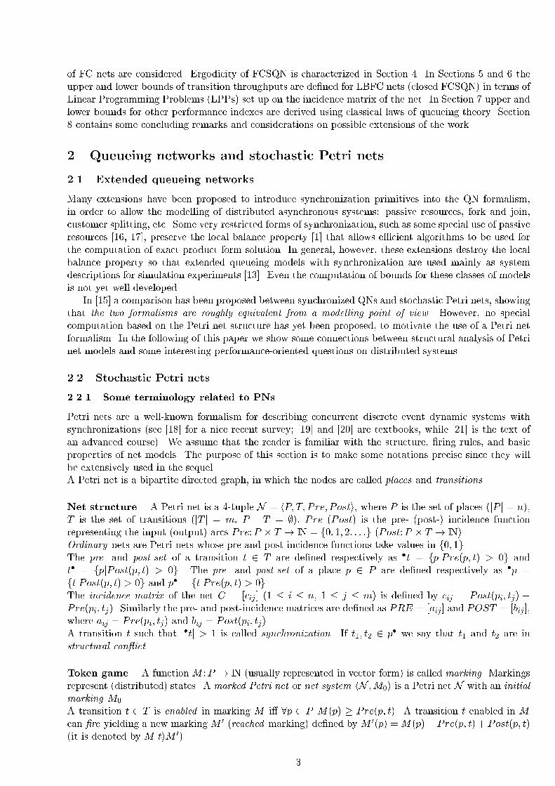
of FC nets are considered. Ergodicity of FCSQN is characterized in Section 4. In Sections 5 and 6 theupper and lower bounds of transition throughputs are de�ned for LBFC nets (closed FCSQN) in terms ofLinear Programming Problems (LPPs) set up on the incidence matrix of the net. In Section 7 upper andlower bounds for other performance indexes are derived using classical laws of queueing theory. Section8 contains some concluding remarks and considerations on possible extensions of the work.2 Queueing networks and stochastic Petri nets2.1 Extended queueing networksMany extensions have been proposed to introduce synchronization primitives into the QN formalism,in order to allow the modelling of distributed asynchronous systems: passive resources, fork and join,customer splitting, etc. Some very restricted forms of synchronization, such as some special use of passiveresources [16, 17], preserve the local balance property [1] that allows e�cient algorithms to be used forthe computation of exact product form solution. In general, however, these extensions destroy the localbalance property so that extended queueing models with synchronization are used mainly as systemdescriptions for simulation experiments [13]. Even the computation of bounds for these classes of modelsis not yet well developed.In [15] a comparison has been proposed between synchronized QNs and stochastic Petri nets, showingthat the two formalisms are roughly equivalent from a modelling point of view. However, no specialcomputation based on the Petri net structure has yet been proposed, to motivate the use of a Petri netformalism. In the following of this paper we show some connections between structural analysis of Petrinet models and some interesting performance-oriented questions on distributed systems.2.2 Stochastic Petri nets2.2.1 Some terminology related to PNsPetri nets are a well-known formalism for describing concurrent discrete event dynamic systems withsynchronizations (see [18] for a nice recent survey; [19] and [20] are textbooks, while [21] is the text ofan advanced course). We assume that the reader is familiar with the structure, �ring rules, and basicproperties of net models. The purpose of this section is to make some notations precise since they willbe extensively used in the sequel.A Petri net is a bipartite directed graph, in which the nodes are called places and transitions.Net structure. A Petri net is a 4-tuple N = hP; T; Pre; Posti, where P is the set of places (jP j = n),T is the set of transitions (jT j = m, P \ T = ;), Pre (Post) is the pre- (post-) incidence functionrepresenting the input (output) arcs Pre:P � T ! IN = f0; 1; 2; : : :g (Post:P � T ! IN).Ordinary nets are Petri nets whose pre and post incidence functions take values in f0; 1g.The pre- and post-set of a transition t 2 T are de�ned respectively as �t = fpjPre(p; t) > 0g andt� = fpjPost(p; t) > 0g. The pre- and post-set of a place p 2 P are de�ned respectively as �p =ftjPost(p; t) > 0g and p� = ftjPre(p; t) > 0g.The incidence matrix of the net C = [cij ] (1 � i � n, 1 � j � m) is de�ned by cij = Post(pi; tj) �Pre(pi; tj). Similarly the pre- and post-incidence matrices are de�ned as PRE = [aij ] and POST = [bij],where aij = Pre(pi; tj) and bij = Post(pi; tj).A transition t such that j�tj > 1 is called synchronization. If t1; t2 2 p� we say that t1 and t2 are instructural con ict.Token game. A function M :P ! IN (usually represented in vector form) is called marking. Markingsrepresent (distributed) states. A marked Petri net or net system hN ;M0i is a Petri net N with an initialmarking M0.A transition t 2 T is enabled in marking M i� 8p 2 P M(p) � Pre(p; t). A transition t enabled in Mcan �re yielding a new marking M 0 (reached marking) de�ned by M 0(p) =M(p)� Pre(p; t) +Post(p; t)(it is denoted by M [tiM 0). 3

A sequence of transitions � = t1t2 : : : tn is a �ring sequence of hN ;M0i i� there exists a sequence ofmarkings such that M0[t1iM1[t2iM2 : : : [tniMn. In this case, markingMn is said to be reachable fromM0by �ring �, and this is denoted by M0[�iMn. M [�i denotes a �rable sequence � from marking M . Thefunction ~�:T ! IN is the �ring count vector of the �rable sequence �, i.e., ~�(t) represents the numberof occurrences of t 2 T in �. If M0[�iM , then we can write in vector form M = M0 + C � ~�, which isreferred to as the linear state equation of the net. The reachability set R(N ;M0) is the set of all markingsreachable from the initial marking.Basic properties. A place p 2 P is said to be k{bounded i� 8M 2 R(N ;M0), M(p) � k. A markednet hN ;M0i is said to be (marking) k{bounded i� each of its places is k{bounded, and it is boundedi� it is k{bounded for some k 2 IN. A marked net is said to be safe i� it is 1{bounded. A net N isstructurally bounded i� 8M0 the marked nets hN ;M0i are bounded.Given an initial marking, an implicit place [22] is one which never is the only place that restricts the�ring of its output transitions. Let N be any net and Np be the net resulting from adding an implicitplace p to N . Therefore, the �ring sequences in hN ;M0i and hNp;M0 [m0(p)i are identical.A transition t 2 T is live in hN ;M0i i� 8M 2 R(N ;M0), 9M 0 2 R(N ;M) such that M 0 enables t. Themarked net hN ;M0i is live i� all its transitions are live (i.e., liveness of the net guarantees the possibilityof an in�nite activity of all transitions). A net N is structurally live i� 9M0 such that the marked nethN ;M0i is live. The marked net hN ;M0i is deadlock-free i� 8M 2 R(N ;M0) 9t 2 T such thatM enablest. A marked net has a deadlock i� it is not deadlock-free.A consistent component (or T-semi ow) is a function (vector) X:T ! IN such that X 6= 0 and C �X = 0.A conservative component (or P-semi ow) is a function (vector) Y :P ! IN such that Y 6= 0 andY T � C = 0. The support of (T- and P-) semi ows is de�ned by jjXjj = ft 2 T jX(t) > 0g andjjY jj = fp 2 P jY (p) > 0g. A (T- or P-) semi ow I has minimal support i� there exist no other semi- ow I 0 such that jjI 0jj � jjIjj. A (T- or P-) semi ow is canonical i� the greatest common divisor of itscomponents is 1. A (T- or P-) semi ow is elementary i� it is canonical and has minimal support.A net N is consistent if there exists a T-semi ow X � ~1 (where ~1 is a vector with all entries equal to 1).A net N is conservative if there exists a P-semi ow Y � ~1.Net subclasses. The following are classical ordinary net subclasses, characterized by local structuralproperties:- State machines (SM) are ordinary nets such that 8t 2 T : j�tj = jt�j = 1. State machines allow themodelling of decisions (con icts) and concurrency (whenPp2P M0(p) � 2) but not synchronization.- Marked graphs (MG) are ordinary nets such that 8p 2 P : j�pj = jp�j = 1. Marked graphs allowthe modelling of concurrency and synchronization, but not of con ict.- Free choice (FC) nets are ordinary nets such that 8p 2 P : jp�j > 1) �(p�) = fpg. Free choice nets(see, e.g., [10, 11, 12]) allow both synchronization and con ict but in a restricted and disciplinedway. In an FC net, if a place has a shared output transition then it is the only output transition ofthis place. And, equivalently, if a transition has a shared input place then it is the only input placeof this transition. FC nets do not allow the modelling of mutual exclusion semaphores. Throughoutthe paper we consider live and bounded FC nets (LBFC nets).- Simple nets are ordinary nets such that each transition has at most one shared input place, i.e.,8t 2 T; jfp 2 �t : jp�j > 1gj � 1. Simple nets allow the modelling of decisions, concurrency,synchronization, and shared resources (mutual exclusion schemes), but they do not allow coupledshared resources.The following is a net subclass characterized by global structural properties:- Mono-T-semi ow nets [9] are structurally bounded nets with a unique minimal T-semi ow X, thatcontains all transitions. Thus, they verify rank(C) = m � 1, with C the incidence matrix of thenet and m = jT j. 4

2.2.2 On stochastic Petri netsIn the original de�nition, Petri nets did not include the notion of time, and tried to model only thelogical behaviour of systems by describing the causal relations existing between events. This approachshowed its power in the speci�cation and analysis of concurrent systems in a non-interleaved way, i.e., ina primitive way independent of the concept of time. Nevertheless the introduction of timing speci�cationis essential if we want to use this class of models for an evaluation of the performance of distributedsystems.Timing and �ring process. Since Petri nets are bipartite graphs, historically there have been twoways of introducing the concept of time in them, namely, associating a time interpretation with eitherplaces [23] or transitions [24]. Since transitions represent activities that change the state (marking) ofthe net, it seems natural to associate a duration with these activities (transitions). The latter has beenour choice.In order to solve con icts among transitions, two alternatives have been proposed: either a \timed�ring" of transitions in three phases (which changes the �ring rule of Petri nets introducing a timed phasein which the transition is \working" after having removed tokens from the input places and before addingtokens to the output arcs) or a \timed enabling" followed by an atomic �ring (which does not a�ect theusual Petri net �ring rule). A more detailed discussion of the timing and �ring process can be found in[7]. These di�erent timing interpretations have di�erent implications on the resolution of con icts. Sincein the context of this work we are considering FC nets, any con ict can be resolved in a local way byspecifying the routing rates of tokens at places with several output transitions; thus we are not forced tochoose one particular �ring mechanism.We consider both timed and immediate transitions. Timed transitions model services while imme-diate transitions are used to model decisions (routing rates are associated with them). Both timed andimmediate transitions can be used to model synchronizations. Even if the following constraint can berelaxed, for simplicity it is assumed that there do not exist circuits containing only immediate transitions.For each p 2 P with more than one output transition: p� = ft1; :::; tkg, we assume that these transitionsare immediate (i.e., they �re in zero time); the constants r1; :::; rk 2 IN+ are explicitly de�ned in thenet interpretation in such a way that when t1; :::; tk are enabled, transition ti (i = 1; : : : ; k) �res withprobability (or with long run rate, in the case of deterministic con icts resolution policy) ri=(Pkj=1 rj).Note that the routing rates are assumed to be strictly positive, i.e., all possible outcomes of any con icthave a non-null probability of �ring. This fact guarantees a locally fair behaviour for the non-autonomousPetri nets that we consider (a marked net is said to be locally fair i� all output transitions of a sharedplace that are simultaneously enabled in�nitely many times will �re in�nitely often).Concerning the transitions that are neither synchronizations nor in con ict (i.e., t 2 T such that�t = fpg; p� = ftg), an (almost surely) �nite non-null time is associated with each one of them (enablingtime). The absence of con ict for these transitions assures a persistent service, i.e., no customer can leavean initiated service (preemption is not considered).Single versus multiple server semantics. Another possible source of confusion in the de�nition ofthe timing interpretation of a Petri net model is the concept of \degree of enabling" of a transition (or re-entrance). In the case of timing associated with places, it seems quite natural to de�ne an unavailabilitytime which is independent of the total number of tokens already present in the place, and this can beinterpreted as an \in�nite server" policy from the point of view of queueing theory. In the case of timeassociated with transitions, it is less obvious a-priori whether a transition enabled k times in a markingshould work at conditional throughput 1 or k times the one it would work in the case it was enabledonly once. In the case of stochastic Petri nets with exponentially distributed �ring times associated withtransitions, the usual implicit hypothesis is to have \single server" semantics (see, e.g., [25, 26]), andthe case of \multiple server" is handled as a case of �ring rate dependent on the marking; this trickcannot work in the case of other probability distributions. This is the reason why people working withdeterministic timed transition Petri nets prefer an in�nite server semantics (see, e.g., [27, 28]). Of coursean in�nite server transition can always be constrained to a \k{server" behaviour by just reducing its5

q1

t1 e1

r12

r13

q2

q3

t2

t3

q

s

t e

q1

t1 e1

r12

r13

q2

q3

t2

t3

s2

s3

(a)

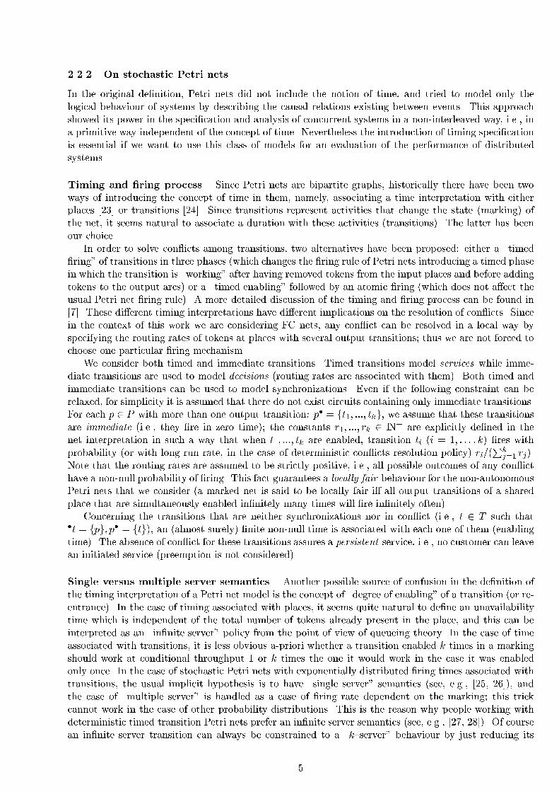
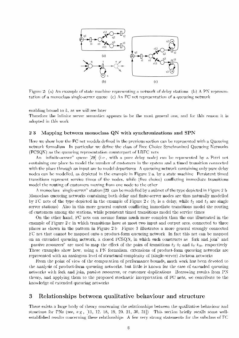
(b) (c)Figure 2: (a) An example of state machine representing a network of delay stations. (b) A PN represen-tation of a monoclass single-server queue. (c) An FC net representation of a queueing network.enabling bound to k, as we will see later.Therefore the in�nite server semantics appears to be the most general one, and for this reason it isadopted in this work.2.3 Mapping between monoclass QN with synchronizations and SPNHere we show how the FC net models de�ned in the previous section can be represented with a Queueingnetwork formalism. In particular we de�ne the class of Free Choice Synchronized Queueing Networks(FCSQN) as the queueing representation counterpart of LBFC nets.An \in�nite-server" queue [29] (i.e., with a pure delay node) can be represented by a Petri netcontaining one place to model the number of customers in the system and a timed transition connectedwith the place through an input arc to model departures. A queueing network containing only pure delaynodes can be modelled, as depicted in the example in Figure 2.a, by a state machine. Persistent timedtransitions represent service times of the nodes, while (free choice) con icting immediate transitionsmodel the routing of customers moving from one node to the other.A monoclass \single-server" station [29] can be modelled by a subnet of the type depicted in Figure 2.b.Monoclass queueing networks containing both delay and �nite-server nodes are thus naturally modelledby FC nets of the type depicted in the example of Figure 2.c (t1 is a delay, while t2 and t3 are singleserver stations). Also in this more general context con icting immediate transitions model the routingof customers among the stations, while persistent timed transitions model the service times.On the other hand, FC nets can assume forms much more complex than the one illustrated in theexample of Figure 2.c in which transitions have at most two input and output arcs, connected to threeplaces as shown in the pattern in Figure 2.b. Figure 3 illustrates a more general strongly connectedFC net that cannot be mapped onto a product-form queueing network. In fact this net can be mappedon an extended queueing network, a closed FCSQN, in which such constructs as \fork and join" and\passive resources" are used to map the e�ect of the pairs of transitions t2{t7 and t9{t10, respectively.These examples show how, using a PN formalism, extensions of product-form queueing networks arerepresented with an analogous level of structural complexity of (single-server) Jackson networks.From the point of view of the computation of performance bounds, much work has been devoted tothe analysis of product-form queueing networks, but little is known for the case of extended queueingnetworks with fork and join, passive resources, or customer duplications. Borrowing results from PNtheory, and applying them to the proposed stochastic interpretation of FC nets, we contribute to theknowledge of extended queueing networks.3 Relationships between qualitative behaviour and structureThere exists a large body of theory concerning the relationships between the qualitative behaviour andstructure for PNs (see, e.g., [11, 12, 18, 19, 20, 21, 30, 31]). This section brie y recalls some well-established results concerning these relationships. A few very strong statements for the subclass of FC6

C=3

C

t1

t2

t9

t4

t3

t5

t6

t10

t7 t8

FJ

A

RA F

1

2

R

JFigure 3: A more general FC net and the corresponding FCSQN.nets are grouped in Section 3.2. Section 3.1 recalls two general results on PNs plus one devoted to thesubclass of mono-T-semi ow.3.1 Three relationshipsStructural boundedness has a nice algebraic characterization (of polynomial time complexity):Theorem 3.1 [21, 30, 18] N is structurally bounded i� 9Y 2 (IN+)n such that Y T � C � 0.Obviously, if N is conservative (i.e., 9Y 2 (IN+)n; Y T � C = 0) then it is structurally bounded. Thefollowing is a su�cient condition for consistency, conservativity, and strong connectivity.Theorem 3.2 [18, 20] Let N be a structurally live and structurally bounded Petri net, then N is consis-tent and conservative. Moreover, if N is connected, it is strongly connected.The last statement of this section concerns mono-T-semi ow nets (that are bounded by de�nition):Theorem 3.3 [9] Let N be a mono-T-semi ow net.1. Deadlock-freeness and liveness are equivalent properties (i.e., either all transitions are live or noneof them is live).2. N is strongly connected.3.2 A brief review of structural theory for LBFC netsThis section introduces a minimum of qualitative results from the large body of FC net theory [10, 11,12, 32, 33, 34, 35]. Additional qualitative results are derived from the quantitative/performance basedapproach introduced in this paper. This fact clearly points out the interest of interleaving the qualitativeand quantitative theories.Let N = hP; T; Pre; Posti be a Petri net and P 0 � P . N 0 = hP 0; T 0; P re0; P ost0i is called a P-component of N i� N 0 is the subnet of N generated by P 0 (i.e., T 0 � T and Pre0; P ost0 are the restrictionsof Pre; Post to P 0 and T 0) and 8t 2 T 0 : j�t \ P 0j � 1 ^ jt� \ P 0j � 1. The next result follows from thewell-known Hack's Theorem [10]. 7

p1

p3

p4

p5

p6 p7

t3 t4

t1 t2p2

Figure 4: A live and bounded simple net: the addition of a token to p5 kills the net (sequence � = t4leads to a deadlock).Theorem 3.4 (A �rst liveness characterization) [32] Let hN ;M0i be a marked FC net. hN ;M0i islive and bounded i�: (a) N is structurally live and structurally bounded, and (b) every P-component ofN is marked at M0.Structure theory of FC nets assures [35] that each minimal P-semi ow of a structurally live and struc-turally bounded FC net generates a P-component. Therefore, the next result can be derived.Theorem 3.5 (An algebraic characterization of liveness) Let N be a structurally live and struc-turally bounded FC net. hN ;M0i is a live marked net i� all its P-semi ows are marked (i.e., 8Y � 0such that Y T � C = 0; Y T �M0 > 0).Proof. If hN ;M0i is live, since it is also bounded then all its P-components are marked (by Theorem3.4). If Y is a P-semi ow of N , its support includes (or is equal to) the support of a minimal P-semi ow,thus it includes the places of a P-component, hence Y is marked. Conversely, if all (and, in particular,the minimal) the P-semi ows are marked, then all the P-components are marked and the net is live(Theorem 3.4). }Corollary 3.1 (Liveness monotonicity) If hN ;M0i is an LBFC net and M 00 � M0 then hN ;M 00i islive.The above corollary is a direct consequence of Theorem 3.5. Nevertheless, it must be pointed out thatit holds also without assuming boundedness [12] (as a consequence of Commoner's Theorem). Livenessmonotonicity does not hold for more general classes of nets (e.g., simple nets, Figure 4).Given a place p of a marked net, the maximum number of tokens at this place over all reachablemarkings is called the marking bound of p (denoted B(p)). The structural counterpart of this conceptcan be de�ned in terms of a linear programming problem (LPP) as follows:De�nition 3.1 (Structural marking bound, SB) Let hN ;M0i be a marked Petri net, 8p 2 PSB(p) def= maximize M(p)subject to M =M0 + C � ~�M � 0; ~� � 0 (LPP1)It is clear that M0[�iM implies M =M0+C � ~� � 0 with ~� � 0. Since the reverse is not true in general,SB(p) is greater than or equal to B(p). The structural marking bound can always be reached in anLBFC net:Theorem 3.6 [32] Let hN ;M0i be an LBFC net, then 8p 2 P;B(p) = SB(p).Corollary 3.2 A live FC net is bounded i� it is structurally bounded.The importance of the above result lies in the fact that structural boundedness can be algebraicallycharacterized (Theorem 3.1).A home state is a marking that may be reached from all other reachable markings. Vogler provedthat an LBFC net has at least one home state: 8

Theorem 3.7 (Home state existence)[33] Let hN ;M0i be an LBFC net. Then hN ;M0i has a homestate.The importance of this result from the performance evaluation point of view is stressed in the nextsection.4 Ergodicity of closed free choice synchronized QNsIn order to speak of steady-state performance we have to assume that some kind of \average behaviour"can be estimated on the long run of the system we are studying. The usual assumption in this case isthat the system models must be ergodic, meaning that at the limit when the observation period tendsto in�nity, the estimates of average values tend (almost surely) to the theoretical expected values of the(usually unknown) probability distributions that characterize the performance indexes of interest.This assumption is very strong and di�cult to verify in general; moreover, it creates problems whenwe want to include the deterministic case as a special case of a stochastic model [9]. Thus we also usethe concept of weak ergodicity that allows the estimation of long run performance even in the case ofdeterministic models.De�nition 4.1 (Ergodicity) Let X� be a stochastic process (or deterministic as a special case), where� represents the time.i) X� is said to be weakly ergodic (or measurable in long run) i� the following limit exists:X def= lim�!1 1� Z �0 Xs ds <1ii) X� is said to be strongly ergodic i� the following condition holds:lim�!1 1� Z �0 Xs ds = lim�!1E[X� ] <1; a.s.For stochastic Petri nets, weak ergodicity of the marking and the �ring processes can be de�ned in thefollowing terms:De�nition 4.2 The marking process of a stochastic marked net is weakly ergodic i� the following limitexists: M def= lim�!1 1� Z �0 Ms ds < ~1and M is called the limit average marking.The �ring process of a stochastic marked net is weakly ergodic i� the following limit exists:~�� def= lim�!1 ~��� < ~1and ~�� is the limit �ring ow vector (in both cases, the initial marking M0 is a given deterministic vectorand � represents the time).The usual (strong) ergodicity concepts [26] are de�ned in the obvious way taking into considerationDe�nition 4.1.ii.Theorem 4.1 Let hN ;M0i be a stochastic LBFC net.1. Both the marking and the �ring processes of hN ;M0i are weakly ergodic.2. If hN ;M0i is semi-Markovian, then the marking and the �ring processes are strongly ergodic.9

Proof. For LBFC nets, the existence of home state is assured (Theorem 3.7). Then, after a possibletransient phase, the system state is always trapped in a unique strongly connected �nite subset of thestate space (terminal class). Thus, the marking and �ring processes are weakly ergodic.If semi-Markovian LBFC nets are considered (stochastic LBFC nets whose marking process is semi-Markov) strong ergodicity of the marking and �ring processes is assured. This is because the existence ofhome state implies that only one proper closed subset of the state space exists and it has �nite cardinality.Therefore, the Markov chain restricted to that subset is irreducible and positive recurrent, hence stronglyergodic. }In other words, for LBFC nets it makes sense to speak of a unique steady-state behaviour and tocompute bounds for the performance of this steady-state.5 Upper bounds for the throughput of LBFC netsIn this Section, upper bounds for the throughput of LBFC nets are presented. First we derive somegeneral results from the structural theory of nets, and then we specialize the problem to MGs and FCnets.5.1 General approach and MGs caseLet us take into account just the �rst moments of the Probability Distribution Functions (PDFs, forshort) associated with transitions. In the following, let �i be the mean value of the random variableassociated with the �ring of transition ti. The limit �ring ow vector per time unit (under weak ergodicityassumption) is ~�� = lim�!1 ~��=� and the mean time between two consecutive �rings of a selectedtransition ti (mean cycle time of ti), �i = 1=~��i .In what follows, the relative �ring frequency vector or vector of visit ratios to transitions (i.e., thelimit �ring ow vector ~�� normalized for having the ith component equal 1) is denoted byFi def= �i~��Obviously, the above de�nition makes no sense if a deadlock is reachable. In this case ~�� = 0 or, in otherwords, the cycle time �i is in�nite for all transitions.The following Little's formula [29] for stochastic Petri nets [26] holds under weak ergodicity assump-tion: M(pi) = PRE(pi) �R(pi)~��where M(pi) is the limit mean marking of place pi, PRE(pi) is the ith row of the pre-incidence matrix,and R(pi) is the mean response time at place pi (i.e., the mean sojourn time of tokens: sum of the waitingtime and the service time). The response times at places are unknown but can be lower-bounded fromthe knowledge of the mean �ring time associated with transitions:M � PRE �D � ~�� (1)where D is the diagonal matrix with elements �i; i = 1; : : : ;m. From this inequality, a lower bound �lbifor the mean cycle time associated with transition ti can be derived. We take into account that �lbi mustbe such that inequality (1) holds for every place pj :�lbi � PRE(pj) �D � FiM(pj) (2)Since the vector M is unknown, (2) cannot be solved. However, taking the product with a P-semi ow Yfor any reachable marking M : Y T �M0 = Y T �M = Y T �M (3)Now, from (1) and (3): �iY T �M0 � Y T � PRE �D � Fi10

p1

p3p4

p5

t3

t4

t1

t2

p2

p1

p3

t3 t4

t1 t2

p2

p4

p5

r1 r2

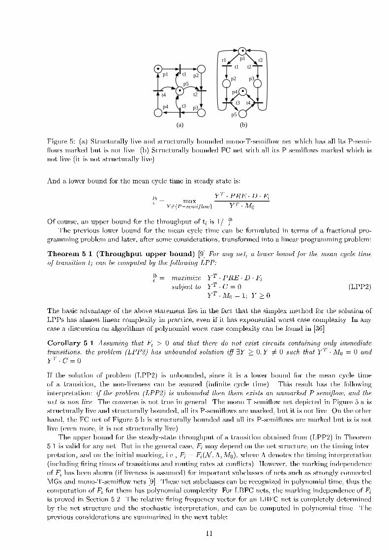
(a) (b)Figure 5: (a) Structurally live and structurally bounded mono-T-semi ow net which has all its P-semi- ows marked but is not live. (b) Structurally bounded FC net with all its P-semi ows marked which isnot live (it is not structurally live).And a lower bound for the mean cycle time in steady state is:�lbi = maxY 2fP�semiflowg Y T � PRE �D � FiY T �M0Of course, an upper bound for the throughput of ti is 1=�lbi .The previous lower bound for the mean cycle time can be formulated in terms of a fractional pro-gramming problem and later, after some considerations, transformed into a linear programming problem:Theorem 5.1 (Throughput upper bound) [9] For any net, a lower bound for the mean cycle timeof transition ti can be computed by the following LPP:�lbi = maximize Y T � PRE �D � Fisubject to Y T � C = 0Y T �M0 = 1; Y � 0 (LPP2)The basic advantage of the above statement lies in the fact that the simplex method for the solution ofLPPs has almost linear complexity in practice, even if it has exponential worst case complexity. In anycase a discussion on algorithms of polynomial worst case complexity can be found in [36].Corollary 5.1 Assuming that Fi > 0 and that there do not exist circuits containing only immediatetransitions, the problem (LPP2) has unbounded solution i� 9Y � 0; Y 6= 0 such that Y T �M0 = 0 andY T � C = 0.If the solution of problem (LPP2) is unbounded, since it is a lower bound for the mean cycle timeof a transition, the non-liveness can be assured (in�nite cycle time). This result has the followinginterpretation: if the problem (LPP2) is unbounded then there exists an unmarked P-semi ow, and thenet is non-live. The converse is not true in general. The mono-T-semi ow net depicted in Figure 5.a isstructurally live and structurally bounded, all its P-semi ows are marked, but it is not live. On the otherhand, the FC net of Figure 5.b is structurally bounded and all its P-semi ows are marked but is is notlive (even more, it is not structurally live).The upper bound for the steady-state throughput of a transition obtained from (LPP2) in Theorem5.1 is valid for any net. But in the general case, Fi may depend on the net structure, on the timing inter-pretation, and on the initial marking, i.e., Fi = Fi(N ;�;M0), where � denotes the timing interpretation(including �ring times of transitions and routing rates at con icts). However, the marking independenceof Fi has been shown (if liveness is assumed) for important subclasses of nets such as strongly connectedMGs and mono-T-semi ow nets [9]. These net subclasses can be recognized in polynomial time, thus thecomputation of Fi for them has polynomial complexity. For LBFC nets, the marking independence of Fiis proved in Section 5.2. The relative �ring frequency vector for an LBFC net is completely determinedby the net structure and the stochastic interpretation, and can be computed in polynomial time. Theprevious considerations are summarized in the next table:11

m5p1 p5 p3

p2 p4

t1 t3

t2t4

(r1) (r3)

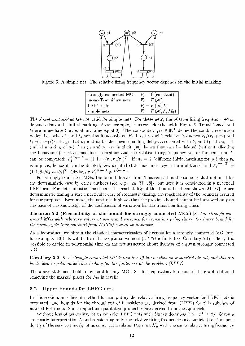
(θ2) (θ4)Figure 6: A simple net. The relative �ring frequency vector depends on the initial marking.strongly connected MGs Fi = ~1 (constant)mono-T-semi ow nets Fi = Fi(N )LBFC nets Fi = Fi(N ;�)simple nets Fi = Fi(N ;�;M0)The above conclusions are not valid for simple nets. For these nets, the relative �ring frequency vectordepends also on the initial marking. As an example, let us consider the net in Figure 6. Transitions t1 andt3 are immediate (i.e., enabling time equal 0). The constants r1; r3 2 IN+ de�ne the con ict resolutionpolicy, i.e., when t1 and t3 are simultaneously enabled, t1 �res with relative frequency r1=(r1 + r3) andt3 with r3=(r1 + r3). Let �2 and �4 be the mean enabling delays associated with t2 and t4. If m5 = 1(initial marking of p5) then p1 and p3 are implicit [30], hence they can be deleted (without a�ectingthe behaviour!); a state machine is obtained and the relative �ring frequency vector for transition t1can be computed: F (m5=1)1 = (1; 1; r3=r1; r3=r1)T . If m5 = 2 (di�erent initial marking for p5) then p5is implicit, hence it can be deleted; two isolated state machines (cycles) are obtained and F (m5=2)1 =(1; 1; �2=�4; �2=�4)T . Obviously F (m5=1)1 6= F (m5=2)1 .For strongly connected MGs, the bound derived from Theorem 5.1 is the same as that obtained forthe deterministic case by other authors (see, e.g., [24, 37, 38]), but here it is considered in a practicalLPP form. For deterministic timed nets, the reachability of this bound has been shown [24, 37]. Sincedeterministic timing is just a particular case of stochastic timing, the reachability of the bound is assuredfor our purposes. Even more, the next result shows that the previous bound cannot be improved only onthe base of the knowledge of the coe�cients of variation for the transition �ring times.Theorem 5.2 (Reachability of the bound for strongly connected MGs) [8] For strongly con-nected MGs with arbitrary values of mean and variance for transition �ring times, the lower bound forthe mean cycle time obtained from (LPP2) cannot be improved.As a byproduct, we obtain the classical characterization of liveness for a strongly connected MG (see,for example, [18]). It will be live i� the optimal value of (LPP2) is �nite (see Corollary 5.1). Then, it ispossible to decide in polynomial time on the net structure about liveness of a given strongly connectedMG.Corollary 5.2 [8] A strongly connected MG is non live i� there exists an unmarked circuit, and this canbe decided in polynomial time looking for the �niteness of the problem (LPP2).The above statement holds in general for any MG [18]. It is equivalent to decide if the graph obtainedremoving the marked places for M0 is acyclic.5.2 Upper bounds for LBFC netsIn this section, an e�cient method for computing the relative �ring frequency vector for LBFC nets ispresented, and bounds for the throughput of transitions are derived from (LPP2) for this subclass ofmarked Petri nets. Some important qualitative properties are derived from the approach.Without loss of generality, let us consider LBFC nets with binary decisions (i.e., jp�j � 2). Given astochastic interpretation � and considering only the relative �ring frequencies at con icts (i.e., indepen-dently of the service times), let us construct a related Petri net NR with the same relative �ring frequency12

vector as the original net. For each pair of transitions in con ict in N , t1 and t2, let r1; r2 2 IN+ be theconstants de�ning the resolution policy, in such a way that when t1 and t2 are enabled, the transitionti �res with probability (or long run rate) ri=(r1 + r2); i = 1; 2. In NR, this resolution policy is summa-rized by the following regulation circuit: �1; �2 2 PR such that ��1 = ��2 = ft2g, ��1 = ��2 = ft1g, andPre(�1; t1) = Post(�2; t1) = r2, Post(�1; t2) = Pre(�2; t2) = r1. Even if the structural con ict betweent1 and t2 remains in NR, the added regulation circuit assures the same relative �ring frequency of bothtransitions in the limiting behaviour, therefore it reduces the non-determinism of the original net.Lemma 5.1 Let hN ;M0i be a live and structurally bounded FC net and � a stochastic interpretation ofN .1. The net NR, de�ned above from N , is mono-T-semi ow.2. With a su�ciently large number of tokens in the places of the regulation circuits (i.e., enoughnumber of tokens for making the regulation circuits live in isolation) and the initial marking in therest of places equal M0, the marked net hNR;MR0 i is live.Proof. 1) N is structurally live and structurally bounded, thus it is strongly connected, consistent, andconservative (Theorem 3.2). By construction, NR is strongly connected, consistent and conservative.NR has at most one consistent component because all the output transitions of a con ict in N mustbelong to a unique consistent component in NR. Since NR is consistent, it has at least a consistentT-semi ow, thus, NR is mono-T-semi ow.2) For a given live marked net, any local scheduling at con icts preserves deadlock-freeness. Then thenet hNR;MR0 i is deadlock-free. Finally, for mono-T-semi ow nets, liveness and deadlock-freeness coincide(Theorem 3.3). }Theorem 5.3 (Marking independence of Fi for structurally bounded and structurally liveFC nets) Let N be a structurally bounded and structurally live FC net and � a stochastic interpretationof N . For all M0 making the net live, Fi = Fi(N ;�) and Fi(t) > 0;8t 2 T .Proof. Let us consider the related net hNR;MR0 i. It has the same relative �ring frequency vector asthe original net (since the net is live, transitions t1 and t2 can be �red in�nitely often, and their relativefrequency is de�ned by the rates r1 and r2). It is mono-T-semi ow (Lemma 5.1) and its limiting behaviourfor the �ring count process is de�ned by the unique T-semi ow XR > 0 (see [9]).Finally, Fi = XR=XR(ti), and since XR > 0 and it depends only on NR, i.e., on N and � (in fact, onthe con ict resolution rates), then Fi = Fi(N ;�) > 0. }The relative �ring frequency vector Fi for a given transition ti of the structurally bounded nethNR;MR0 i must be a consistent component [31]:CR � Fi = 0; Fi > 0; Fi(ti) = 1 (4)But CR = (CT jRT j�RT )T , where R is a matrix with a�n rows (a =Pp2P;t2T Pre(p; t); i.e., the numberof arcs in Pre) derived from the con icts resolution policy: each row of R gives an independent relationbetween the throughput of two transitions in free con ict. And equation (4) is equivalent to:i) C � Fi = 0 (i.e., Fi is a consistent component of C; n equations)ii) R � Fi = 0 (i.e., the routing rates are respected; a� n equations)iii) Fi > 0 (i.e., the relative �ring frequency between any pair of transitions Fi(tj)=Fi(tk) is �nite)iv) Fi(ti) = 1 (i.e., the vector is normalized for having the ith component equal 1)The above system can be rewritten in a more compact way: CR !Fi = 0; Fi > 0; Fi(ti) = 1 (5)The following observations about the previous system can be done:13

1. The system (5) has at most one solution (Lemma 5.1).2. If (5) has no solution then the net is structurally non-live and sooner or later it will reach a deadlock.This follows from the fact that if system (4) has no solution, then NR has no consistent componentand the net cannot have any in�nite behaviour [31]. See, for example, the net in Figure 5.b. Forr1 = 1; r2 = 2, the system (5) has no solution, and the net is structurally non-live.3. The existence of solution for system (5) is a necessary but non-su�cient condition for the structuralliveness of N . This can be easily checked using once again the net in Figure 5.b. For r1 = r2 = 1,there exists a solution of system (5): Fi = (1; 1; 1; 1)T , but the FC net is structurally non-live!The open question from the previous considerations is: When a strongly connected and structurallybounded FC net is structurally live? The answer is given by the next theorem.Theorem 5.4 (Algebraic characterization of structural liveness for strongly connected struc-turally bounded FC nets) Let N be a strongly connected and structurally bounded FC net and C itsincidence matrix.1. N is structurally live i� rank(C) = m� 1� (a� n).2. N is structurally non-live i� rank(C) � m� (a� n).where n = jP j;m = jT j, and a =Pp2P;t2T Pre(p; t).Proof. 1) If N is strongly connected, structurally live, and structurally bounded then NR is stronglyconnected, structurally live, and structurally bounded and has one T-semi ow, i.e., it is mono-T-semi- ow. Thus rank(CR) = m � 1. And this is true for all (locally fair) con ict resolution rates. Thenm� 1 = rank(CR) = rank(C)+ rank(R) = rank(C)+ a�n, i.e., rank(C) = m� 1� (a�n). Note thatrank(CR) = rank(C) + rank(R) because none of the places of the regulation circuits can be implicit: ifone of them was implicit, the choice in the original net would not be free, against the hypothesis.If rank(C) = m�1�(a�n), the system (5) has solution for all con ict resolution policies (the numberof independent equations is rank(C) plus rank(R) = a� n plus one, for the normalization equation; thenumber of variables is m). This leads to claim that under any locally fair con ict resolution policy,in�nite behaviours in which all transitions �re (Fi > 0) can always be obtained for a large enough initialmarking and no deadlock can be reached. In other words, the net is structurally live.2) If N is a strongly connected and structurally bounded FC net and C its incidence matrix, thenrank(C) � m�1�(a�n). This result follows considering once more the derived netNR. It is equivalent tosee that rank(CR) � m�1, i.e., the net NR has not more than one consistent component. And this is truebecause each pair of output transitions of a given place that could generate two consistent componentsare related with a regulation circuit, thus they should belong to the same consistent component.Now, statement 2 of this theorem follows from statement 1 and from the fact that rank(C) � m �1� (a� n). }The classical duality result for free choice nets [10] can be derived from the previous theorem. Thereverse dual of a net is obtained by changing places by transitions (dual) and reversing the arc orientation(reverse). The reader can check that the reverse dual of an FC net is also an FC net. If C (Crd) is theincidence matrix of N (Nrd), it is easy to verify that Crd = �CT . Therefore rank(C) = rank(Crd).Corollary 5.3 (Duality theorem) Let N = hP; T; Pre; Posti be an FC net. N is structurally live andstructurally bounded i� the reverse-dual of N ;Nrd = hT; P; Post; P rei, is structurally live and structurallybounded.Proof. If N is structurally live and structurally bounded then it is strongly connected, consistent,and conservative (Theorem 3.2). Then Nrd is strongly connected, consistent, and conservative, thusstructurally bounded.Finally rank(C) = rank(Crd) and mrd � 1� (ard � nrd) = n� 1� (a�m) = m� 1� (a� n), i.e., ifN is structurally live then Nrd is also structurally live. }Two well-known results of structural theory of nets, can also be deduced from the previous results:14

Corollary 5.4 (Structural liveness in FC net subclasses)1. Strongly connected MGs are structurally live nets.2. Strongly connected state machines are structurally live nets.In fact, for the MG case, strong connection is not needed (an MG is live i� all circuits are marked, i.e.,there always exists an initial marking making the MG live [18]).Now, from Theorem 5.1 and from the fact that the relative �ring frequency vector can be computedin polynomial time for LBFC nets (Theorem 5.3), the next result follows:Corollary 5.5 (Polynomial complexity) For strongly connected and structurally bounded FC nets,the computation of the lower bound for the mean cycle time of a transition given by Theorem 5.1 hasworst case polynomial complexity on the net size.Proof. Step 1) Both the strong connectivity and the structural boundedness of a net can be characterizedin polynomial time. FC nets are also characterized in polynomial time. Thus the subclass of nets whichare referred to in the statement are characterized in polynomial time.Step 2) For this subclass of nets, the computation of the relative �ring frequency vector Fi is polyno-mial, solving the system (5).Step 3) Finally, from the knowledge of Fi, the lower bound for the mean cycle time of transition tican be computed, solving the problem (LPP2), thus in polynomial time. }As in the case of strongly connected MGs, a characterization of liveness for structurally live andstructurally bounded FC nets can be derived.Corollary 5.6 (Liveness characterization) Assuming that Fi > 0 and that there do not exist circuitscontaining only immediate transitions, liveness of structurally live and structurally bounded FC nets canbe decided in polynomial time, checking the boundedness of the problem (LPP2).Proof. For FC nets, both structural boundedness (Theorem 3.1) and structural liveness in structurallybounded nets (Theorem 5.4) are polynomial problems. The optimal value of (LPP2) is a lower boundfor the mean cycle time. If this optimal value is in�nite the mean cycle time is unbounded so the net isnon live. If the optimal value of (LPP2) is �nite, this means that for all Y � 0 such that Y T � C = 0,then Y T �M0 > 0. In other words, all P-semi ows are marked, thus the net is live (Theorem 3.5). }This result is nothing more but the \natural" generalization of the existence of an unmarked circuitfor strongly connected MGs (Corollary 5.2). It does not hold for non-FC nets and for non live FC nets.The throughput upper bound derived from (LPP2) is not reachable in general for LBFC nets. Severalimprovements and a reachable bound for the case of live and safe FC nets can be found in [34].Linear programming problems give an easy way to derive results and interpret them. Just looking atthe problem (LPP2) the following monotonicity property is obtained.Corollary 5.7 (Performance bound monotonicity) Let hN ;M0i be an LBFC net and � the mean�ring times vector.1. For a �xed �, if M 00 � M0 (i.e., increasing the number of initial resources) then the throughputupper bound of hN ;M 00; �i is greater than or equal to the one of hN ;M0; �i (i.e., �lb0 � �lb).2. For a �xed M0, if �0 � � (i.e., for faster resources) then the throughput upper bound of hN ;M0; �0iis greater than or equal to the one of hN ;M0; �i (i.e., �lb0 � �lb).We conjecture that the above monotonicity properties hold, in fact, for the exact throughput of LBFCnets. Nevertheless, the �rst is not true for live and bounded simple nets: remember that the addition oftokens (i.e., resources) to a live and bounded simple net can make it non-live (see Figure 4).15

t1 t2

t3

p1 p2

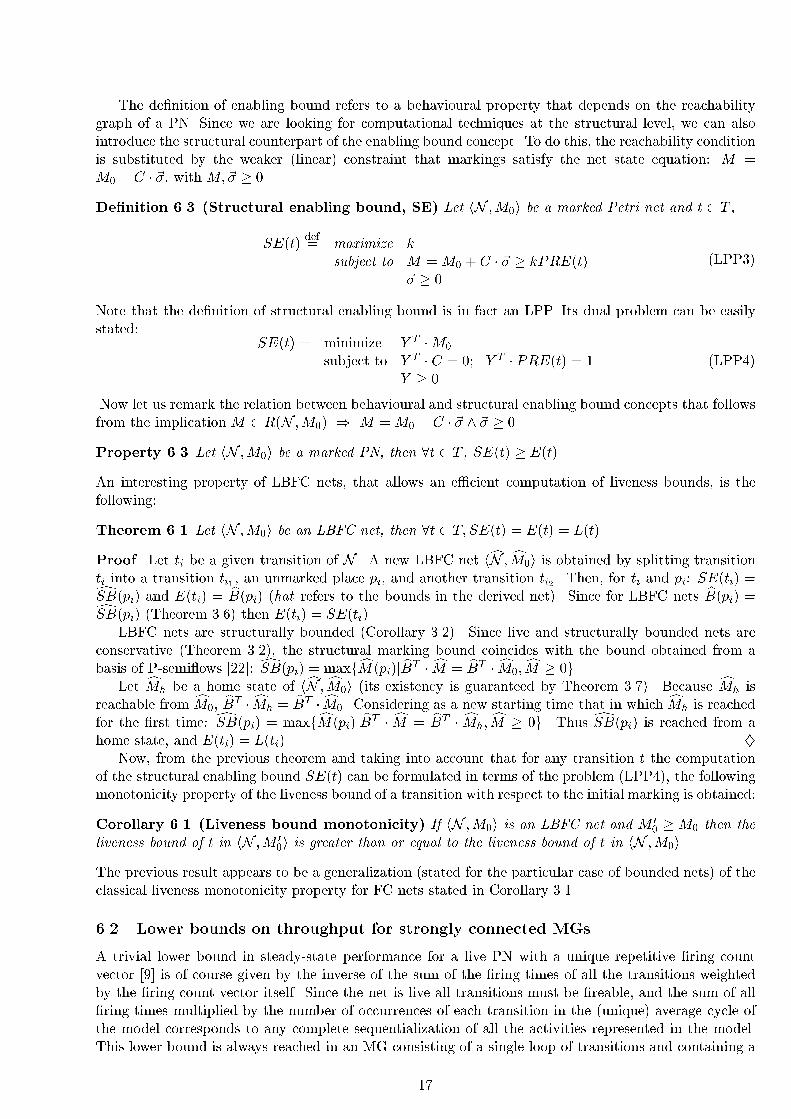
p32Figure 7: A net with enabling bound greater than liveness bound for transition t1.6 Lower bounds for the throughput of LBFC netsIn this section, lower bounds on throughput are proposed, independent of the higher moments of the�ring delay PDFs, based on the computation of the transition liveness bounds. First we introduce theliveness bound concept as a generalization of the concept of liveness of a transition, and some relatedresults.Liveness bound is a measure of the maximum degree of enabling of a transition. The degree of enablingof transition t in a marking M is the minimum among all the input places p 2 �t of the integer part ofM(p)=Pre(p; t). It identi�es the number of activities associated to the transition that could potentiallyprogress concurrently, disregarding con icts, at a given marking.6.1 Additional liveness concepts and resultsThe performance of a model with in�nite server semantics depends on the maximum degree of enablingof the transitions; and in particular, the steady-state performance depends on the maximum degreeof enabling of transitions in steady-state, which in general can be di�erent from the maximum degreeof enabling of a transition during its evolution starting from the initial marking. For this reason weintroduce here two concepts of degree of enabling of a transition t: the enabling bound E(t), and theliveness bound L(t). The last is obviously constrained to the steady-state. They allow to generalize theclassical concepts of enabling and liveness of a transition.De�nition 6.1 (Enabling bound, E) Let hN ;M0i be a marked Petri net and t 2 T , E(t) def=maxfkj9M 2 R(N ;M0) :M � kPRE(t)g.De�nition 6.2 (Liveness bound, L) Let hN ;M0i be a marked PN and t 2 T , L(t) def= maxfkj8M1 2R(N ;M0);9M 2 R(N ;M1) : M � kPRE(t)g.From the above de�nitions it appears clear how it is possible to obtain a k{server transition from anin�nite server one: adding one place that is both input and output for that transition and marking itwith k tokens. The following is also obvious from the de�nition.Property 6.1 Let hN ;M0i be a marked PN, then 8t 2 T , E(t) � L(t).A case of strict inequality in this Property can be interpreted as a generalization of the concept of non-liveness: there exist transitions containing \potential servers" that are never used in the steady-state;these additional servers might only be used in a transient phase, so they \die" during the evolution ofthe model. See, as an example, the net in Figure 7. It is decision-free but not free choice (it is not anordinary net), and E(t1) > L(t1) (E(t1) = 2 and L(t1) = 1). On the other hand it is not di�cult to seethat the condition L(t) > 0 is equivalent to the usual liveness condition for transition t.Since for any reversible net (i.e., such that M0 is a home state) the reachability graph (which is adirected labelled graph) is strongly connected, the following can be stated.Property 6.2 Let hN ;M0i be a reversible PN, then 8t 2 T , E(t) = L(t).As a particular case, live MGs are reversible, so that enabling and liveness bounds are equal for them.16

The de�nition of enabling bound refers to a behavioural property that depends on the reachabilitygraph of a PN. Since we are looking for computational techniques at the structural level, we can alsointroduce the structural counterpart of the enabling bound concept. To do this, the reachability conditionis substituted by the weaker (linear) constraint that markings satisfy the net state equation: M =M0 + C � ~�, with M;~� � 0.De�nition 6.3 (Structural enabling bound, SE) Let hN ;M0i be a marked Petri net and t 2 T ,SE(t) def= maximize ksubject to M =M0 + C � ~� � kPRE(t)~� � 0 (LPP3)Note that the de�nition of structural enabling bound is in fact an LPP. Its dual problem can be easilystated: SE(t) = minimize Y T �M0subject to Y T � C = 0; Y T � PRE(t) = 1Y � 0 (LPP4)Now let us remark the relation between behavioural and structural enabling bound concepts that followsfrom the implication M 2 R(N ;M0) ) M =M0 + C � ~� ^ ~� � 0.Property 6.3 Let hN ;M0i be a marked PN, then 8t 2 T , SE(t) � E(t).An interesting property of LBFC nets, that allows an e�cient computation of liveness bounds, is thefollowing:Theorem 6.1 Let hN ;M0i be an LBFC net, then 8t 2 T; SE(t) = E(t) = L(t).Proof. Let ti be a given transition of N . A new LBFC net hcN ; cM0i is obtained by splitting transitionti into a transition ti1 , an unmarked place pi, and another transition ti2 . Then, for ti and pi: SE(ti) =dSB(pi) and E(ti) = bB(pi) (hat refers to the bounds in the derived net). Since for LBFC nets bB(pi) =dSB(pi) (Theorem 3.6) then E(ti) = SE(ti).LBFC nets are structurally bounded (Corollary 3.2). Since live and structurally bounded nets areconservative (Theorem 3.2), the structural marking bound coincides with the bound obtained from abasis of P-semi ows [22]: dSB(pi) = maxfcM (pi)j bBT � cM = bBT � cM0; cM � 0g.Let cMh be a home state of hcN ; cM0i (its existency is guaranteed by Theorem 3.7). Because cMh isreachable from cM0, bBT � cMh = bBT � cM0. Considering as a new starting time that in which cMh is reachedfor the �rst time: dSB(pi) = maxfcM(pi)j bBT � cM = bBT � cMh; cM � 0g. Thus dSB(pi) is reached from ahome state, and E(ti) = L(ti). }Now, from the previous theorem and taking into account that for any transition t the computationof the structural enabling bound SE(t) can be formulated in terms of the problem (LPP4), the followingmonotonicity property of the liveness bound of a transition with respect to the initial marking is obtained:Corollary 6.1 (Liveness bound monotonicity) If hN ;M0i is an LBFC net and M 00 � M0 then theliveness bound of t in hN ;M 00i is greater than or equal to the liveness bound of t in hN ;M0i.The previous result appears to be a generalization (stated for the particular case of bounded nets) of theclassical liveness monotonicity property for FC nets stated in Corollary 3.1.6.2 Lower bounds on throughput for strongly connected MGsA trivial lower bound in steady-state performance for a live PN with a unique repetitive �ring countvector [9] is of course given by the inverse of the sum of the �ring times of all the transitions weightedby the �ring count vector itself. Since the net is live all transitions must be �reable, and the sum of all�ring times multiplied by the number of occurrences of each transition in the (unique) average cycle ofthe model corresponds to any complete sequentialization of all the activities represented in the model.This lower bound is always reached in an MG consisting of a single loop of transitions and containing a17

single token in one of the places, independently of the higher moments of the PDFs (this observation canbe trivially con�rmed by the computation of the upper bound, which in this case gives the same value).This trivial lower bound has been improved in [8], based on the knowledge of the liveness bound L(t)for all transitions t of the MG.Theorem 6.2 (Throughput lower bound for strongly connected MGs and its reachability)[8] For any live and bounded MG with a speci�cation of the mean �ring times �j for each tj 2 T it is notpossible to assign PDFs to the transition �ring times such that the average cycle time is greater than�ub = mXj=1 �jL(tj) = mXj=1 �jSE(tj)independently of the topology of the net.Moreover, this upper bound for the mean cycle time is reachable for any MG topology and for someassignement of PDFs to the �ring delay of transitions (i.e., the bound cannot be improved).MGs are a subclass of FC nets. According to Theorem 6.1, the liveness bound equals the structuralenabling bound for each transition (see also [8]); thus the problem of the determination of the structuralenabling bound can be characterized in terms of the problem (LPP4), which is known to be solvable inpolynomial time. The optimum of the objective function is always achieved with elementary P-semi owsY . In case of MGs, these elementary P-semi ows can only be elementary cycles, so that we can givethe following interpretation of the LPP in net terms: the liveness bound for a transition t of a stronglyconnected MG is given by the minimum number of tokens contained in any cycle containing transition t.6.3 Lower bounds on throughput for LBFC netsThe non-trivial lower bound for the throughput of MGs (dividing by the liveness bound) presented inSection 6.2 can be applied now in the following way: weighting the mean �ring time of tj , �j, with thecomponent of the relative �ring ow vector Fi(tj), for each transition.Theorem 6.3 (Throughput lower bound for LBFC nets) For any LBFC net with a speci�cationof the mean �ring times �j for each tj 2 T it is not possible to assign PDFs to the transition �ring timessuch that the average cycle time of transition ti is greater than�ubi = mXj=1 Fi(tj)L(tj) �j = mXj=1 Fi(tj)SE(tj)�jindependently of the topology of the net, where Fi is the relative �ring frequency vector with Fi(ti) = 1.Proof. Let us consider a deterministic con icts resolution policy. A strongly connected MG with thesame relative �ring frequency vector can be constructed as follows (in fact, since for the MG Fi = ~1,what can appear are several instances of transitions to get the Fi of the original net):1. Steady-state markings must be home states. Let Mh be one of the home states (there always existsome for LBFC nets, according to Theorem 3.7), and substitute it to the initial marking (i.e.,hN ;Mhi is reversible).2. From the LBFC net, a safe marking can be derived preserving liveness, removing tokens from Mh.3. Develop the process, resolving the con icts with the deterministic given policy, until cyclicity ap-pears (see [24]) and the relative �ring frequency holds. A safe MG is obtained in which transitionsappear according to their relative �ring frequencies.4. The rest of tokens at each place in Mh in the original LBFC net, can be added now in the corre-sponding place of the MG. 18

The actual cycle time of the original FC net (with deterministic con icts resolution policy) is less thanor equal to the one of the derived MG because the behaviour of the net has been constrained. Now,apply the bound obtained in Theorem 6.2. Di�erent instances of a given transition are considered in therelative rate of the corresponding component in the relative �ring frequency vector. Thus, the boundobtained for the derived MG applying Theorem 6.2 coincides with the bound obtained for the originalnet using the formula stated in this theorem. The theorem follows because L(tj) = SE(tj) for LBFCnets (Theorem 6.1). }Note that the structural enabling bound of a transition can be computed by means of an LPP, whichis known to be solvable in polynomial time, thus the above lower bound for the throughput of LBFC netscan be computed in polynomial time on the net structure.7 Bounds for other performance indexesFrom the knowledge of upper and lower bounds for the steady-state throughput of transitions and fromwell-known queueing theory laws (such as Little's formula) [29] fast bounds for other performance indexesof interest can be derived.7.1 Bounds for the mean length of queuesIn this section, a fast computation of upper and lower bounds for the limit mean marking of places (i.e.,length of queues including the customers in service) is proposed.In Section 5.1 the following inequality was derived from Little's formula for stochastic PNs:M � PRE �D � ~��where D is the diagonal matrix with elements �i (mean �ring time associated with transition ti; i =1; : : : ;m). Then, a lower bound for the mean marking of places in steady-state can be computed, fromthe knowledge of a lower bound for the throughput of transitions.Theorem 7.1 For any LBFC net with a speci�cation of the mean �ring times associated with transitionsand of the con ict resolution policy, it is not possible to assign PDFs to the transition �ring times suchthat the mean marking of places in steady-state is less thanM lb = PRE �D � ~�lbwhere ~�lb is a lower bound for the throughput vector (i.e., ~�lb(ti) = 1=�ubi ; i = 1; : : : ;m, with �ubi theupper bound for the mean cycle time of ti computed in Theorem 6.3).For the computation of an upper bound for the mean marking of a given place p1 in steady-state, let usconsider a P-semi ow Y = (Y1; : : : ; Yn)T whose support includes this place (i.e., Y1 6= 0). We haveY T �M0 = Y T �MTherefore Y T �M0 � Y1M(p1) + (Y2; : : : ; Yn) � (M lb(p2); : : : ;M lb(pn))TM(p1) �M lb(p1) + 1Y1Y T � (M0 �M lb)and the same condition holds for each P-semi ow including place p1. Then, the computation of an upperbound for the mean marking of places can be formulated in terms of an LPP as follows:Mub(p) = minimize M lb(p) + Y T � (M0 �M lb)subject to Y T � C = 0;Y T � ep = 1;Y � 0where ep = (0; : : : ; 0; p̂1 ; 0; : : : ; 0)T , and the restriction Y T � ep = 1 allows us to omit the denominator Ypwhich is assumed to be non null.The bound can also be computed from a dual version of the previous problem. Because LBFC nets areconservative, the dual problem is equivalent to the following one, that admits a nice direct interpretation.19

Theorem 7.2 For any live and bounded free choice net with a speci�cation of the mean �ring timesassociated with transitions and of the con ict resolution policy, it is not possible to assign PDFs to thetransition �ring times such that the mean marking of place p in steady-state is greater thanMub(p) = maximize M(p)subject to BT �M = BT �M0; M �M lbwhere the rows of BT are a basis of the left annullers of C.In this problem, the maximum mean marking of place p is computed, subject to the following restrictions:the mean marking must satisfy the place invariant equations, and it must be greater than or equal to thelower bound computed in Theorem 7.1.7.2 Maximum capacity of queuesAn interesting information for the designer is the maximum capacity of queues that is needed for theexecution of the processes from the �xed initial state. This information can be used for giving a correctdimension of the model implementation. For live and bounded free choice nets, it is possible to computein polynomial time on the net size, the exact maximum marking that can be reached from the initialstate in each place, solving an LPP. This is based on the fact that the behavioural bound of p, B(p), isequal to the structural bound, SB(p) (Theorem 3.6).Because LBFC nets are conservative, the problem (LPP1) that de�nes SB(p) can be easily rewrittenleading to the following statement:Theorem 7.3 For LBFC nets, the reachable marking bound of places coincides with the structural mark-ing bound obtained solving the following LPP:SB(p) = maximize M(p)subject to BT �M = BT �M0; M � 0with BT a basis of the left annullers of C.The reader is invited to compare the LPPs in Theorems 7.2 and 7.3. The �rst is more constrained(M �M lb � 0), therefore as expected, Mub(p) � SB(p) = B(p).7.3 Other computable boundsUsing fundamental laws of queueing theory [29], bounds for other performance �gures can be computed.As an example, let us consider the computation of bounds for the mean response time at places.The mean response time R(pi) at a place pi is the mean value of the sojourn time of a token in thisplace (i.e., sum of waiting plus service time). From the knowledge of upper and lower bounds for thethroughput of transitions and for the mean marking of places, and applying Little's law, upper and lowerbounds for the response time at places can be deduced as follows:Rub(pi) = Mub(pi)PRE(pi) � ~�lbRlb(pi) = PRE(pi) �D � FkPRE(pi) � Fkwhere ~�lb and Mub are the bounds computed in previous sections.20

8 ConclusionsAmong the main achievements of this work the following can be stressed: (1) it is a starting point fora performance evaluation (i.e., quantitative) theory for free choice synchronized queueing networks, amodel class that generalizes many proposals of QN extensions; (2) the theory is developed in a uni�edframework considering qualitative and quantitative properties; and (3) from the quantitative approach,classical and new qualitative fundamental properties of FC nets appear in a simple and straightforwardway.The extensive bibliography of this work may be surprising at a �rst glance, but it can be justi�edbecause one of our primary goals was to try to deeply bridge two active �elds: Petri nets (in particular,free choice nets) qualitative theory and stochastic models (stochastic nets and extensions of queueingnetworks) theory. The bene�ts have been for both the qualitative and quantitative understanding of suchmodels. From the qualitative point of view, some unexpected fundamental new results allow the linearalgebra-based characterization of liveness in FC nets. These results strongly in uenced the introductionof a new linear algebra based perspective of qualitative theory of LBFC nets [39]. An extension of thenecessary condition in the rank theorem for general nets has been presented in [40]. From the quantitative(performance analysis) point of view, fast algorithms (polynomial complexity) allow to compute boundsfor throughput for a class of synchronized QNs for which ergodicity is assured. From the above boundsand classical fundamental queueing theory laws, some derived performances (as queue bounds) can alsobe computed in polynomial time.Among the \natural" extensions of this work, we can point out two, presently under consideration:relaxing the topology of nets (synchronized QNs) and considering open free choice synchronized monoclassqueueing networks.Acknowledgements. The authors wish to thank J. M. Colom, J. Esparza, and J. Mart��nez from theUniversity of Zaragoza for many useful discussions.References[1] F. Baskett, K. M. Chandy, R. R. Muntz, and F. Palacios. Open, closed, and mixed networks ofqueues with di�erent classes of customers. Journal of the ACM, 22(2):248{260, April 1975.[2] Proceedings of the International Workshop on Timed Petri Nets, Torino, Italy, July 1985. IEEE-Computer Society Press.[3] Proceedings of the International Workshop on Petri Nets and Performance Models, Madison, WI,USA, August 1987. IEEE-Computer Society Press.[4] Proceedings of the 3rd International Workshop on Petri Nets and Performance Models, Kyoto, Japan,December 1989. IEEE-Computer Society Press.[5] J. R. Jackson. Jobshop-like queueing systems. Management Science, 10(1):131{142, October 1963.[6] J. Campos and M. Silva. Steady-state performance evaluation of totally open systems of Markoviansequential processes. In M. Cosnard and C. Girault, editors, Decentralized Systems, pages 427{438.Elsevier Science Publishers B.V. (North-Holland), Amsterdam, The Netherlands, 1990.[7] M. Ajmone Marsan, G. Balbo, A. Bobbio, G. Chiola, G. Conte, and A. Cumani. The e�ect ofexecution policies on the semantics and analysis of stochastic Petri nets. IEEE Transactions onSoftware Engineering, 15(7):832{846, July 1989.[8] J. Campos, G. Chiola, J. M. Colom, and M. Silva. Tight polynomial bounds for steady-stateperformance of marked graphs. In Proceedings of the 3rd International Workshop on Petri Nets andPerformance Models, pages 200{209, Kyoto, Japan, December 1989. IEEE-Computer Society Press.21

[9] J. Campos, G. Chiola, and M. Silva. Ergodicity and throughput bounds of Petri nets with uniqueconsistent �ring count vector. IEEE Transactions on Software Engineering, 17(2):117{125, February1991.[10] M. H. T. Hack. Analysis of production schemata by Petri nets. M. S. Thesis , TR-94, M.I.T.,Boston,USA, 1972.[11] P. S. Thiagarajan and K. Voss. A fresh look at free choice nets. Information and Control, 61(2):85{113, May 1984.[12] E. Best. Structure theory of Petri nets: The free choice hiatus. In W. Brawer, W. Reisig, andG. Rozenberg, editors, Advances in Petri Nets 1986 - Part I, volume 254 of LNCS, pages 168{205.Springer-Verlag, Berlin, 1987.[13] C. H. Sauer, E. A. MacNair, and J. F. Kurose. The research queueing package: past, present, andfuture. In Proceedings of the 1982 National Computer Conference. AFIPS, 1982.[14] F. Baccelli and A. Makowski. Queueing models for systems with synchronization constraints. Pro-ceedings of the IEEE, 77(1):138{161, January 1989.[15] M. Vernon, J. Zahorjan, and E. D. Lazowska. A comparison of performance Petri nets and queueingnetwork models. In Proceedings of the 3rd International Workshop on Modelling Techniques andPerformance Evaluation, pages 181{192, Paris, France, March 1987. AFCET.[16] M. Ajmone Marsan, G. Balbo, G. Chiola, and S. Donatelli. On the product-form solution of a classof multiple-bus multiprocessor system models. Journal of Systems and Software, 6(1,2):117{124,May 1986.[17] J.Y. Le Boudec. A BCMP extension to multiserver stations with concurrent classes of customers.In Proceedings of PERFORMANCE'86 and ACM SIGMETRICS, Raleigh, NC, USA, May 1986.[18] T. Murata. Petri nets: Properties, analysis, and applications. Proceedings of the IEEE, 77(4):541{580, April 1989.[19] J.L. Peterson. Petri Net Theory and the Modeling of Systems. Prentice-Hall, Englewood Cli�s, NJ,USA, 1981.[20] M. Silva. Las Redes de Petri en la Autom�atica y la Inform�atica. Editorial AC, Madrid, 1985. InSpanish.[21] W. Brauer, W. Reisig, and G. Rozenberg, editors. Advances in Petri Nets 1986, volume 254 and255 of LNCS. Springer-Verlag, Berlin, 1987.[22] J. M. Colom and M. Silva. Improving the linearly based characterization of P/T nets. In G. Rozen-berg, editor, Advances in Petri Nets 1990, volume 483 of LNCS, pages 113{145. Springer-Verlag,Berlin, 1991.[23] J. Sifakis. Use of Petri nets for performance evaluation. Acta Cybernetica, 4(2):185{202, 1978.[24] C. Ramchandani. Analysis of Asynchronous Concurrent Systems by Petri Nets. PhD thesis, MIT,Cambridge, MA, USA, February 1974.[25] M. K. Molloy. Performance analysis using stochastic Petri nets. IEEE Transaction on Computers,31(9):913{917, September 1982.[26] G. Florin and S. Natkin. Les r�eseaux de Petri stochastiques. Technique et Science Informatiques,4(1):143{160, February 1985. In French. 22

[27] W. M. Zuberek. Performance evaluation using timed Petri nets. In Proceedings of the InternationalWorkshop on Timed Petri Nets, pages 272{278, Torino,Italy, July 1985. IEEE-Computer SocietyPress.[28] M. A. Holliday and M. Vernon. A generalized timed Petri net model for performance analysis. IEEETransactions on Software Engineering, 13(12):1297{1310, December 1987.[29] L. Kleinrock. Queueing Systems Volume I: Theory. John Wiley & Sons, New York, NY, USA, 1975.[30] M. Silva and J. M. Colom. On the computation of structural synchronic invariants in P/T nets. InG. Rozenberg, editor, Advances in Petri Nets 1988, volume 340 of LNCS, pages 386{417. Springer-Verlag, Berlin, 1988.[31] M. Silva. Towards a synchrony theory for P/T nets. In K. Voss, H. Genrich, and G. Rozenberg,editors, Concurrency and Nets, pages 435{460. Springer-Verlag, Berlin, 1987.[32] J. Esparza. Structure Theory of Free Choice Nets. PhD thesis, Departamento de Ingenier��a El�ectricae Inform�atica, Universidad de Zaragoza, Spain, June 1990. Research Report GISI-RR-90-03.[33] W. Vogler. Live and bounded free choice nets have home states. Petri Net Newsletter, 32:18{21,April 1989.[34] J. Campos. Performance Bounds for Synchronized Queueing Networks. PhD thesis, Departamentode Ingenier��a El�ectrica e Inform�atica, Universidad de Zaragoza, Spain, December 1990. ResearchReport GISI-RR-90-20.[35] E. Best and J. Desel. Partial order behaviour and structure of Petri nets. Formal Aspects ofComputing, 2(2):123{138, 1990.[36] G. L. Nemhauser, A. H. G. Rinnooy Kan, and M. J. Todd, editors. Optimization, volume 1 ofHandbooks in Operations Research and Management Science. North-Holland, Amsterdam, 1989.[37] C. V. Ramamoorthy and G. S. Ho. Performance evaluation of asynchronous concurrent systemsusing Petri nets. IEEE Transactions on Software Engineering, 6(5):440{449, September 1980.[38] T. Murata. Use of resource-time product concept to derive a performance measure of timed Petrinets. In Proceedings 1985 Midwest Symposium Circuits and Systems, Louisville, USA, August 1985.[39] J. Esparza and M. Silva. On the analysis and synthesis of free choice systems. In G. Rozenberg,editor, Advances in Petri Nets 1990, volume 483 of LNCS, pages 243{286. Springer-Verlag, Berlin,1991.[40] J. M. Colom, J. Campos, and M. Silva. On liveness analysis through linear algebraic techniques. InProceedings of the Annual General Meeting of ESPRIT Basic Research Action 3148 Design MethodsBased on Nets (DEMON), Paris, France, June 1990.

23