The ‘Concert Queueing Game’ with Feedback Routing

Ruixin Wang

School of Industrial Engineering, Purdue University, West Lafayette IN 47906

Harsha Honnappa∗

School of Industrial Engineering, Purdue University, West Lafayette IN 47906

Abstract

The objective of this paper is to dilate the interplay between feedback routing and strategic arrival

behavior in single class queueing networks. We study a variation of the ‘Network Concert Queueing

Game,’ wherein a fixed but large number of strategic users arrive at a network of queues where

they can be routed to other nodes in the network following a fixed routing matrix, or potentially

fedback to the end of the queue they arrive at. Working in a non-atomic setting, we prove the

existence of Nash equilibrium arrival and routing profiles in three simple, but non-trivial, network

topologies/architectures. In two of them, we also prove uniqueness of the equilibrium. Our results

prove that Nash equilibrium decisions on when to arrive and which queue to join in a network

are substantially impacted by routing, inducing ‘herding’ behavior under certain conditions on

the network architecture. Our theory raises important design implications for capacity-sharing in

systems with strategic users, such as ride-sharing and crowdsourcing platforms.

Keywords: Queueing, Game Theory, Strategic arrivals, Non-atomic equilibrium, routing

1. Introduction

We study the behavior of a finite, but large, number of strategic users in open queueing networks.

Self-interested users choose a time to arrive and a route to take through the network. This type

of behavior is evident in theme parks where users can choose which rides to visit and in which

order, in ride-sharing networks where drivers can choose to visit different geographical locations

at different times of the day and in some desired order, and even crowd-sourcing platforms where

∗Corresponding author.Email addresses: wang2252@purdue.edu (Ruixin Wang), honnappa@purdue.edu (Harsha Honnappa)

Preprint submitted to Elsevier May 23, 2017

users can choose which platform to participate in.

To model this strategic behavior, we study a variation of the ‘Network Concert Queueing Game’

studied in [6], where the Nash equilibrium arrival timing and routing behavior of non-atomic users

was studied in feedforward queueing networks. In the current paper, we consider network topologies

with feedback. We elucidate the impact of feedback routing on strategic behavior by considering

the following three network topologies/architectures 1:

(i) a single server queue where jobs can be repeatedly returned (without bound) to the tail of

the buffer after service,

(ii) a single server queue where a job can only be returned to the tail of the buffer a finite number

of times after service, and

(iii) a two queue network with routing between queue ‘A’ and queue ‘B’, such that a fraction p of

jobs that complete service at queue ‘A’ will be routed to queue ‘B’ and a fraction 1− p will

be directed out of the network (and vice versa from ‘B’ to ‘A’).

Pμ

Pμ>

Pμ2>

Pμ1>

(a) Single Queue, Infinite Returns

Pμ

Pμ>

Pμ2>

Pμ1>

(b) Single Queue, Finite Returns

Pμ

Pμ>

P

μ2>

P

μ1>A

B

(c) Parallel Network with Cross-

Feedback

Figure 1: Network Architectures. Blue circle with arrow head indicates that jobs that have been fedback a fixed

finite number of times are routed out of the network.

See Figure 1 for illustrations. Note that these are the simplest, non-trivial, architectures for

which the equilibrium traffic profile can be computed. We should also note that our focus on the

non-atomic setting helps to avoid modeling issues that arise in the atomic game, that detract from

the broader question we wish to focus on here: what is the impact of feedback and routing on the

equilibrium arrival profile? We note that the three network architectures are in increasing order of

analytical complexity of computing the equilibrium profiles.

1We will use topology and architecture interchangeably henceforth.

2

Following [6], we consider a disutility function that trades off the cost of arriving early against

the cost of waiting in the buffer. However, we modify it to explicitly account for the cost of being

returned to the tail of the queue after service completion. Each user must consider the impact of

these (potential) returns in making a decision of when to arrive and which route to take. Since every

user must make the same calculation, an individuals’ cost is determined through the interaction

of the users. Now, assuming that the non-atomic users strategically choose a time to arrive and a

queue to join (in architecture (iii), specifically) such that their disutility is minimized, we identify

the Nash equilibrium arrival and routing profile. With feedback, users who arrive at time t must

also contend with the fact that they potentially might interact with users who arrive after them.

This makes the equilibrium computation substantially more complicated than the ‘no feedback’

case studied previously whereby users arriving after t would not directly affect the disutility of the

user arriving at t.

While our primary motivation for this paper is mathematical, as noted in the first paragraph of

this introduction, our results are can find application in a number of disparate service systems. As

an example, consider how our results also provide modeling insights into strategic behavior in ride-

sharing platforms such as Uber and Lyft. In particular, we provide a game theoretic explanation of

how drivers might strategically choose a time and location to offer rides. We note, however, that our

interest is in understanding the implications of feedback routing on the computation of equilibrium

strategies, rather than in identifying an accurate model for ride-sharing platforms. To fix the ideas,

consider the two queue first-in-first-out (FIFO) network in Figure 1c. Each queue can be viewed as

a geographical location where drivers offer rides to passengers; drivers are the ‘users’ entering the

queue and passengers are modeled as the single server. Note that the FIFO assumption implies that

users obtain rides in order of their arrival, which is not an unreasonable approximation. On the

other hand, the single server implies that only one passenger will be available to hail a ride at each

time instant. For simplicity, we assume that the service rate is fixed; in effect, this implies that the

number of passengers available to pick up per unit time is fixed. A fixed fraction p of passengers at

queue ‘A’ wish to visit queue ‘B’ (and vice versa), and the remainder 1 − p will exit this network

(implying they will traverse to a different location). We assume that drivers are strategic about

the amount of time they spend awaiting rides, and that this naturally translates into lost revenue.

For the purposes of this discussion, we assume that the lost revenue is linear in the waiting time,

3

and so we focus on a disutility/cost function that is a function of the sojourn time. We assume

that users must make a one-shot decision of when and where to join the system; i.e., we are not

considering a dynamic decision making process. The Nash equilibrium arrival and routing profile

we compute in this paper provides insight into how drivers will react to routing and feedback, and

can be used in capacity analysis and incentive design for ride-sharing networks.

1.1. Results

We start our analysis with the single queue case where a user can be returned to the back of

the queue (potentially) an infinite number of times, as depicted in Figure 1a. This ‘toy’ problem

is mathematically much simpler than the other network architectures we consider. However, it

highlights the impact feedback can have on equilibrium strategies. Since there is a single queue, the

only strategic decision to make is in when to arrive. After establishing the existence of a piecewise-

linear Nash equilibrium arrival profile in Theorem 1, we prove that, modulo a technical condition

on the parameters of the problem, this is the only Nash equilibrium in Theorem 2. Note that this

result is with loss of generality. We find that, as the fraction of users being fedback increases,

at equilibrium users arrive later (though potentially before service starts at time 0) and that the

last user to arrive does so much later. Furthermore, the arrival epoch of the last user increases

super-exponentially as the feedback fraction p approaches 1. Furthermore, the equilibrium arrival

profile is piecewise linear, and we find that the slope of the arrival profile before service starts

to be larger than after. One could interpret this as implying that the arrival ‘rate’ is greater

before service starts than after. Users following the equilibrium strategy introduce additional costs

on others in the form of negative externalities. It is thus useful to compare the social disutility

(computed as an aggregate over the entire population) of following the equilibrium strategy against

the social disutility of following the Pareto optimal strategy suggested by a central planner. We do

this by computing the price of anarchy (PoA), or the ratio of the equilibrium social disutility to

the optimal social disutility, and show that it is precisely equal to 2. This implies that the social

disutility if doubled by following the equilibrium strategy. The PoA computation indicates that

some coordination between users can result in lowered social disutility, though we do not pursue

this line of research here.

Next, we consider a network architecture where users return a finite number of times. As it

turns out, the analysis of the single return case is quite challenging and we focus on that exclusively.

4

We expect the analysis of the single return model to extend to an arbitrary (but finite) number

of returns in a straightforward manner (though we do not pursue it here). Figure 1b depicts the

network architecture we consider; the blue circle represents a decision ‘element’ that only returns

users (with probability p) who have not received a second service. At each time instant t > 0,

the service effort expended up to that point in time includes service rendered to users receiving

their first service and those receiving their second service. Thus, the ‘feedback rate’ is dependent

on the state of the queue, in contrast to the fixed ‘rate’ in the infinite return case. Users fedback

for a second service will not affect the waiting time of users who arrive after the former depart

(clearly). Contrast this with the infinite return case where every user who arrives can potentially

delay all other users, due to the feedback effect. This is the crux of the equilibrium computation

making it substantially more difficult than the infinite return model. In Theorem 4 we prove

the existence of a piecewise linear equilibrium arrival profile by carefully constructing a sequence

of time intervals where fedback users are served and showing that the size of these intervals, as

measured by the Lebesgue measure, satisfy a recursive relationship. Next, in Theorem 5 we prove

that this equilibrium is unique, modulo a technical condition on the parameters of the problem.

Once again, we compute the price of anarchy (PoA) and show that is it equal to 2. In contrast to

the infinite return case, we find that while the equilibrium queue length is linear, the arrival profile

is (only) piecewise linear. Interestingly enough, we observe that the equilibrium arrival profile

displays ‘herding’ behavior whereby users arrive at a ‘high rate’ in a time interval (whose length

is determined by equilibrium considerations), followed by a time interval with a lower rate (again

determined at equilibrium).

As it turns out the the equilibrium computation in the single return case can be extended to the

network topology in Figure 1c. Here an arriving user must not only decide when to arrive, but also

which queue to join. On completion of the first service, a fraction of the served users are routed

to the other queue for a second service, where they join the back of the line. Once the second

service is completed they are routed out of the network. Leveraging the proof of existence for the

equilibrium in the single return case, we prove the existence of a Nash equilibrium arrival profile

in this case as well. Once again, we observe a similar herding behavior at equilibrium. Note that,

this implies that a user arriving at station ‘A’ (say) cannot arbitrarily improve her disutility by

arriving at station ‘B’ instead. However, proving uniqueness of the Nash equilibrium profile turns

5

out to be much more complicated. In Theorem 7 we prove that the Nash equilibrium is unique

provided that the queueing delay faced by a user arriving at time t is equal in either queue. This,

of course, need not be the case in general. The complication in the proof arises from the fact that

the fraction of time server i (= 1, 2) spends serving users routed from server j = mod (i, 2) + 1 is

dependent on the fraction of time server j spends serving users routed from server i. This results in

a rather complicated dependency structure that prevents a straightforward resolution to uniqueness

computation.

Here’s a brief overview of the paper. In Section 2 we present a short literature review of the

relevant prior art. We present our mathematical model of the fluid queueing network in Section 3,

with special attention paid to the workload process. We commence our analysis of the game in

Section 4 with the single queue and infinite return case. In Section 5 we study the single queue and

single return case and leverage these results for the parallel queue/cross-feedback case in Section 6.

We end with a brief summary and discussion of open problems in Section 7.

2. Literature Review

There is a long history of modeling strategic behavior in queueing networks. The book [5] is

an excellent compendium of the existing literature up to 2003. Much of the research effort in this

direction has been focused on strategic behavior in single queues, largely ignoring routing effects.

There is an earlier stream of research initiated by Braess [2] where given fixed routes between two

locations, users must strategically choose a route to take from the first location to the next that

minimizes a delay cost. Another stream of research corresponds to the question of when to arrive

at a queue and how this decision can be regulated. This stream of research was pioneered by Naor

[11]. This paper is closely related to the latter research sequence.

Our investigations are directly motivated by the analysis in [6], where strategic users choose

a time epoch to arrive and a route to take through the network a priori to arrival; this makes

the associated game one-shot. The authors identify the non-atomic Nash equilibrium arrival and

routing profile of the game by showing that, at equilibrium, the network “collapses” to a parallel

queue network. It was noted in that paper that feedback routes could significantly impact the

equilibrium computation. In this paper we do not allow selfish routing (it is probabilistic and

fixed), since our goal is to understand how feedback routing will affect Nash equilibrium arrival

6

and routing decisions. It should be noted that, to the best of our knowledge, besides [6] all of the

remaining literature on arrival timing decisions have concerned single server queues; see [4, 8, 10].

The current paper will be first to study the impact of routing/network topology on equilibrium

strategies.

It is important to contrast the setting of the current paper with another sequence of research

that appears similar. [12] consider a two queue multi-class network, where users must visit both

queues for service. Users strategically choose which sequence of queues to visit, and the authors

prove that the network is unstable when users follow Nash equilibrium strategies. On the other

hand, [1] consider a two queue single class network where, again, the users must visit both queues

in either sequence and strategically route themselves. Under overload conditions, the authors

consider three games: one where a finite number of users are present when service starts and users

sequentially route themselves. Thus each agent responds to the observed decisions made by the

others. In the second game, a finite number of arrivals occur over a short time horizon (thus, there

is order in the arrivals) and finally a game where users arrive according to a Poisson process. Most

interestingly, the authors prove that the price of anarchy in the first game is lower than alternative

routing schemes. In both of these papers, the network topology does not affect the arrival decisions

of the users; they must necessarily visit both stations in sequence. The only strategic decision the

users must make is which sequence of queues to visit. In this paper, users must make that decision

in consort with arrival timing decisions.

3. Mathematical Model

The network architectures we consider are depicted in Figure 1. The queues we consider are

single-class, and are assumed to follow a FIFO service schedule and a non-idling service policy.

We model each queue in the network as a single server fluid queue that offers service rate µ.

We assume that the total volume of non-atomic users arriving at the system is Λ = 1. A pure

strategy for a user c ∈ [0, 1] is simply the arrival epoch tc ∈ (−∞,+∞), and a mixed strategy is a

probability distribution Fc with support in (−∞,+∞). The cumulative strategy profile is defined

as F :=∫ 10 Fcm(dc), where m(·) is the Lebesgue measure. This is, in essence, an average of the

mixed strategies followed by all the users. F (t) is the cumulative number of users who will arrive

to the system by t on average.

7

Consider the feedback queue in Figure 1a. The workload, or virtual waiting time, process, when

each user follows a Nash equilibrium strategy, can be straightforwardly written down as

w(t) =

µ−1F (t) t ≤ 0,

µ−1F (t) + pt− t t > 0.

(1)

This equation follows as a consequence of Lemma 2 in [6] that shows that the server does not idle

when it follows a non-preemptive service policy and the traffic follows an equilibrium strategy. Note

that pµt is the fraction of served users up to time t who are fedback for a repeat service.

Next, in the single return case depicted in Figure 1b, the workload in the system is determined

by the amount of time the server has spent serving users fedback for a second service. Let Ω ⊂ [0,∞)

be the set of all time instants where feedback users are served and let At := s ∈ Ω : s ≤ t. Then,

the workload process is

w(t) =

µ−1F (t) t ≤ 0,

µ−1F (t) + p(t−m(At))− t t > 0,

(2)

where m(·) is the lebesgue measure.

Finally, consider the two queue cross-feedback network. It is beneficial to introduce the 2 × 2

routing matrix P, where the entry pi,j is the fraction of fluid users who are routed from node i to

node j. The workload process at time t is the column vector w(t) = (w1(t), w2(t)), where wi is the

workload in node i. Using the fluid model in [7], it follows that

w(t) =

M−1 (F1(t), F2(t)) t ≤ 0,

M−1 (F1(t), F2(t))− (1, 1)t+ PAt(1, 1), t > 0,

(3)

where M = diag(µ−11 , µ−12 ) is the diagonal matrix of the inverse service rates, and At = diag(t −

A1,t, t − A2,t), where A1,t follows the definition of At in (2) - albeit, A1,t is amount of time spent

serving users routed from queue 2 (and vice-versa).

The cost function/disutility we consider generalizes the cost function introduced in [9] by in-

corporating the expected cost of returning or (potentially) being fedback (in the Figures 1a and

1b) or routed between queues (in Figure 1c). To be precise, the disutility of arriving at time t is

defined as:

8

C(t) = αw(t) + β(t+ w(t)) + γG(t), (4)

where γ > 0 andG(t) is the additional waiting time cost incurred by feedback/routing of users. Note

that we choose to separate the extra waiting cost so that its impact can be explicitly quantified. The

precise form of the additional waiting cost depends on the specific architecture under consideration.

Thus, we delay a full description of the additional cost. Finally, following the description in [6] we

define the equilibrium condition:

Definition 1 (Equilibrium Condition). The cost of arriving at the queue must be a constant in the

support of the equilibrium arrival profile F ?.

4. Single Queue, Infinite Return

We first consider the case where each user can re-enter the queue after service with probability

p and potentially an unbounded number of times. This case is mathematically simpler to study,

but also provides insight into how feedback influences the equilibrium.

4.1. Individual Cost

Every user faces the “risk” of returning after completing service, which increases her overall

waiting time through the queue. We denote the waiting time after the ith service for a (potential)

user arriving at t by Ri(t) and the overall additional waiting time by R(t) =∑Ni

i=1Ri(t), where Ni

is the number of times user i returns. We set R(t) = 0 if a user does not return. Now, let Ti(t) be

the time when the user arriving at time t returns for the ith potential return. We have

T1(t) =

F (t)µ , if t ≤ 0

t+ Q(t)µ , if t > 0,

(5)

and Ti+1(t) = Ti(t) + Q(Ti(t))µ . Consequently, Ri(t) = Q(Ti(t))

µ . Then, the total cost of potential

returns, G(t), is defined as

G(t) :=

∞∑i=1

piRi(t) =

∞∑i=1

piQ(Ti(t))

µ. (6)

9

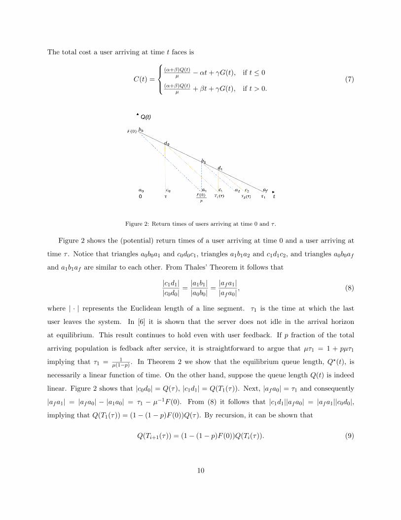
The total cost a user arriving at time t faces is

C(t) =

(α+β)Q(t)

µ − αt+ γG(t), if t ≤ 0

(α+β)Q(t)µ + βt+ γG(t), if t > 0.

(7)

Figure 2: Return times of users arriving at time 0 and τ .

Figure 2 shows the (potential) return times of a user arriving at time 0 and a user arriving at

time τ . Notice that triangles a0b0a1 and c0d0c1, triangles a1b1a2 and c1d1c2, and triangles a0b0af

and a1b1af are similar to each other. From Thales’ Theorem it follows that

|c1d1||c0d0|

=|a1b1||a0b0|

=|afa1||afa0|

, (8)

where | · | represents the Euclidean length of a line segment. τ1 is the time at which the last

user leaves the system. In [6] it is shown that the server does not idle in the arrival horizon

at equilibrium. This result continues to hold even with user feedback. If p fraction of the total

arriving population is fedback after service, it is straightforward to argue that µτ1 = 1 + pµτ1

implying that τ1 = 1µ(1−p) . In Theorem 2 we show that the equilibrium queue length, Q?(t), is

necessarily a linear function of time. On the other hand, suppose the queue length Q(t) is indeed

linear. Figure 2 shows that |c0d0| = Q(τ), |c1d1| = Q(T1(τ)). Next, |afa0| = τ1 and consequently

|afa1| = |afa0| − |a1a0| = τ1 − µ−1F (0). From (8) it follows that |c1d1||afa0| = |afa1||c0d0|,

implying that Q(T1(τ)) = (1− (1− p)F (0))Q(τ). By recursion, it can be shown that

Q(Ti+1(τ)) = (1− (1− p)F (0))Q(Ti(τ)). (9)

10

Now, let q := 1− (1− p)F (0), then for a user (potentially) arriving at time t,

G(t) = pµ−1Q(T1(t))∞∑n=0

(pq)n.

Since pq < 1 it follows that

G(t) =pQ(T1(t))

µ(1− pq). (10)

Finally, from equation (5), (6), (7) and (1), it follows that the cost of arriving at time t is

C(t) =

(α+β)F (t)

µ − αt+γpQ(

F (t)µ

)

µ(1−pq) , if t ≤ 0

(α+β)(F (t)−µt+pµt)µ + βt+

γpQ(t+Q(t)µ

)

µ(1−pq) , if t > 0.

(11)

4.2. Equilibrium Arrival Profile

Let τ0 be the time at which the first arrival occurs and τf the departure time of the last user to

arrive. As noted before, in [6] it is shown that at equilibrium the server does not idle and the last

arrival will not face any waiting time, implying that τf = τ1 = (µ(1− p))−1. Using the equilibrium

condition in Definition 1, the equilibrium cost of arriving at time epoch t in the support of the

support of the equilibrium arrival profile satisfies C(t) = C(τf ) = β(µ(1−p))−1. Note too, that the

support cannot have gaps, else a strategic user could arbitrarily reduce her disutility by arriving at

such a time instant. It follows that the equilibrium support must be [τ0, τf ], and C(τ0) = βµ(1−p) .

Then, (11) and the fact that F (τ0) = 0 imply τ0 = γpF (0)µα(1−pq) −

βµα(1−p) . This leads us to our first

result.

Theorem 1. Suppose Q? is piecewise-linear on (τ0, 0] and (0, τ1) (respectively), then there exists

a piecewise-linear Nash equilibrium arrival profile F ?.

Proof. First, (1) implies that it suffices to find the coefficients of the equilibrium linear queue length

Q? to establish the existence of F ?. Recall, from (7) and (10), that

C(t) =

(α+β)Q?(t)

µ − αt+γpQ?

(Q?(t)µ

)µ(1−pq) , if t ≤ 0

(α+β)Q?(t)µ + βt+

γpQ?(t+

Q?(t)µ

)µ(1−pq) , if t > 0.

Suppose t > 0, then at any Nash equilibrium it follows that

(α+ β)Q?(t)

µ+ βt+

γpQ?(t+ Q?(t)

µ

)µ(1− pq)

− β

µα(1− p)= 0.

11

Suppose Q?(t) = a1t+ a2 for t > 0, where (a1, a2) ∈ R2, then 0 =

t

((α+ β)a1

µ+ β +

γpa1µ(1− pq)

+γpa21

µ2(1− pq)

)+

((α+ β)a2

µ+

γpa2µ(1− pq)

+γpa1a2

µ2(1− pq)− β

αµ(1− p)

).

(12)

It follows that a21γp

µ2(1−pq) + a1

((α+β)µ + γp

µ(1−pq)

)+ β = 0 and a2

(α+βµ + γp

µ(1−pq)

)+ a1a2

γpµ2(1−pq) −

βαµ(1−p) = 0. Note that the former (quadratic) equation is a function of a1 alone. A real-valued

solution for a1 exists if and only if the discriminant satisfies(α+ β

µ+

γp

µ(1− pq)

)2

− 4βγp

µ2(1− pq)≥ 0. (13)

Let a∗1 be the solution of the quadratic equation, then

a∗2 =β

αµ(1− p)

(α+ β

µ− γp

µ(1− pq)+ a∗1

γp

µ2(1− pq)

)−1.

Thus, the equilibrium queue length when t ≥ 0 is Q?(t) = a∗1t+ a∗2, and denote it as Q?(t)|t≥0.

Likewise, at any Nash equilibrium, if t ≤ 0,

(α+ β)Q?(t)

µ− αt+

γpQ?(Q?(t)µ

)µ(1− pq)

− β

µα(1− p)= 0.

Since Q?(t)µ > 0, we use Q∗(t)|t>0 to expand the term γpQ?(·)

µ(1−pq) . Suppose Q?(t) = b1t + b2 for t ≤ 0,

then it follows that

(α+ β)(b1t+ b2)

µ− αt+

γp(a∗1b1t+ a∗1b2)

µ2(1− pq)+

γpa∗2µ(1− pq)

− β

µα(1− p)= 0. (14)

Clearly, b1a∗1

γpµ2(1−pq) + b1

α+βµ − α = 0 and b2

(α+βµ +

γpa∗1µ2(1−pq) + γp

µ(1−pq)

)− β

µα(1−p) = 0. Since we

know that a∗1 and a∗2 exist provided condition (4.2) holds, there exist unique solutions for b∗1 and

b∗2. Thus Q?(t) = b∗1t + b∗2 is the linear equilibrium queue length when t ≤ 0 and we denote it as

Q?(t)|t≤0.

Note that the linear equilibrium arrival profile in Theorem 1 can be expressed as

F ?(t) =

(1− F ?(0))(1− p)µt+ F ?(0), if t > 0

F ?(0)(

βµα(1−p) −

γpF ?(0)µα(1−pq)

)−1t+ F ?(0), if t ≤ 0.

(15)

Thus, it suffices to know the exact expression for F ?(0) to solve for the equilibrium arrival profile.

From (11) it follows that

C(0) =β

µ(1− p)=

(α+ β)F ?(0)

µ+γp((1− F ?(0))(1− p)F ?(0) + pF ?(0))

µ(1− pq).

12

Solving for F ?(0), we obtain

F ?(0) =−√

(βp− γp+ (α+ β)(p− 1))2 − β(4p(α+ β)(p− 1)− 4γp(p− 1)) + γp− βp− (α+ β)(p− 1)

2p(α+ β)(1− p) + 2γp(p− 1).

Our next result proves the (partial) necessity of the linearity of an equilibrium arrival profile

by proving that F ? is unique modulo a condition on the parameters of the cost function.

Theorem 2. F ?(t) is the only Nash equilibrium if (1−p)(α+β)pγ > 1.

First, though, consider the following lemmas.

Lemma 1. The queue length function is continuous at any Nash equilibrium.

Proof. Note that the only discontinuities possible are upwards jumps, on account of (possible)

singularities in the equilibrium arrival profile. Suppose Q?(t) is discontinuous at tx such that

Q?(t+x ) ≤ Q?(t−x ). Then we claim that the user arriving at Q?(t−x ) has an incentive to arrive at

Q?(t+x ) since by delaying her arrival by an infinitesimal amount of time she can reduce her cost.

Thus Q? must necessarily be continuous.

Lemma 2. In any Nash equilibrium, Q?(Tn(t))→ 0 as n→∞.

Proof. Suppose Q?(t0) = 0 for some t0 ∈ [0, τ1), then it is trivial that customers arriving after

t0 will have incentive to switch to t0, which contradicts with the equilibrium condition. Hence,

Q?(t) > 0 for ∀t ∈ [0, τ1). By definition of Ti(t) introduced in equation (5), Ti(t)→ τ1. Since Q?(t)

is a continuous function by lemma 1, Q?(Tn(t))→ 0 as n→∞.

Lemma 3. Let c0 = (α+ β), ci = piγ and a0 = δ 6= 0. For sequence an, if

an =

− 1c0

∞∑j=1

cjaj if n = 0

− 1c0

∞∑j=n+1

cj−naj − 1c0βn−1∑j=0

aj , if n ≥ 1,

(16)

and

0 =∞∑j=0

aj , (17)

then an does not converge to 0 if (1−p)(α+β)pγ > 1.

13

Proof. Suppose an → 0 as n→∞. Then ∀ε→ 0, ∃N1 such that |an| ≤ ε for n > N1. By equation

(16), for n > N1,

−ε < − 1

c0

∞∑j=n+1

cj−naj −β

c0

n−1∑j=0

< − ε

c0

∞∑j=n+1

cj−n −β

c0

n−1∑j=0

aj .

Furthermore, βc0

n−1∑j=0

aj < ε(1− γc0

p1−p). By equation (17), β

c0

n−1∑j=0

aj → 0 as n → ∞. We claim that

ε(1− γc0

p1−p) ≥ 0. Since otherwise, we can find N2 ≥ N1 such that β

c0

n−1∑j=0

aj > ε(1− γc0

p1−p), which

leads to a contradiction. Therefore, an does not converge to 0 if ε(1 − γc0

p1−p) < 0. Since ε > 0 is

arbitrary, it follows that (1−p)(α+β)pγ > 1.

Proof of Theorem 2. Suppose there is another equilibrium F ∗∗(t) with a corresponding queue length

Q∗∗(t), such that Q∗∗(tx) 6= Q?(tx) for some tx. Let δ = Q∗∗(tx)−Q?(tx). Also, let Ti(t) and T ′i (t)

be the time sequences as defined in equation (5) corresponding to Q∗(t) and Q∗∗(t) respectively.

By equation (7) and definition of the equilibrium it follows that

(α+ β)Q∗∗(t)

µ− αt+

∞∑i=1

piγQ∗∗(T ′i (t))

µ=

(α+ β)Q?(t)

µ− αt+

∞∑i=1

piγQ?(Ti(t))

µ, if t ≤ 0,(18)

(α+ β)Q∗∗(t)

µ+ βt+

∞∑i=1

piγQ∗∗(T ′i (t))

µ=

(α+ β)Q?(t)

µ+ βt+

∞∑i=1

piγQ?(Ti(t))

µ, if t > 0.(19)

From equations (18) and (19), we obtain

(α+ β)

(Q∗∗(tx)−Q∗(tx)

)=

∞∑i=1

piγ

(Q?(Ti(tx))−Q∗∗(T ′i (tx))

).

Let a0 = δ, ai = Q?(Ti(tx)) − Q∗∗(T ′i (tx)) for i > 0, c0 = (α + β) and ci = piγ for i > 0.

Substituting in the expression above, we obtain −c0a0 =∑∞

i=1 ciai. Similarly, if we notice that

Ti+1(t)− T ′i+1(t) = µ−1∑i

j=0

(Q∗(Ti(t))−Q∗∗(T ′i (t))

)= µ−1

∑ij=0 aj , then for the users arriving

at time Ti(tx), we have

−c0ai − βi−1∑j=1

aj =∞∑

j=i+1

cj−iaj .

Also, by Lemma 2, Tn(t)→ τ1 and T ′n(t)→ τ1 as n→∞. We, thus, obtain Ti+1(t)− T ′i+1(t) =

µ−1∑i

j=0 aj → 0 as i → ∞, which implies that∑i

j=0 aj → 0 as i → ∞. Applying Lemma 3

it follows that an does not converge to 0 if (1−p)(α+β)pγ > 1. This, however, contradicts Lemma 2

where Q?(Tn(t))→ 0 as n→∞, and further an → 0 as n→∞. Hence, it cannot be the case that

14

Q∗∗(tx) − Q?(tx) = δ 6= 0. Therefore, there does not exist a point tx such that Q∗∗(tx) 6= Q?(tx).

i.e. Q∗∗(t) and Q?(t) must be equal pointwise. Consequently, F ?(t) is the unique Nash equilibrium

arrival profile, provided (1−p)αpγ > 1.

4.3. Price of Anarchy

We define the social cost of following strategy profile F as

J(F ) :=

∫CF (t)dF (t).

Let Jopt denote the social cost of following the optimal arrival profile and Jeq as the social cost

of following the equilibrium arrival strategy profile. It is expected that Jeq will be greater than

Jopt. To characterize the inefficiency of the equilibrium arrival profile, consider the price of anarchy

(PoA) η, defined as:

η = supF∈N

JeqJopt(F )

,

where N is the set of Nash equilibrium profiles. For brevity, let Jeq represent the equilibrium social

cost when the Nash equilibrium strategy is unique.

Theorem 3. The price of anarchy of the single queue, infinite return, arrival game is 2, when

(1−p)(α+β)pγ > 1.

Proof. Let CF ? be the equilibrium disutility of following the unique Nash equilibrium strategy

profile F ?. Recall that CF ?(t) = β(µ(1− p))−1, which implies

Jeq =β

µ(1− p).

Note that we have assumed the total about of arrivals to be 1.

Next, the socially optimal arrival strategy would be to arrange jobs such that they do not face

any delay. In other words, the effective arrival rate, taking the feedback effect into account, should

be equal to the service rate. Let the optimal arrival profile be

F ′opt(t) = µ(1− p)

for t > 0. In this case, the effective arrival rate is∑∞

i=0 µ(1− p)pi = µ. It follows that Copt(t) = βt,

implying

Jopt =

∫ τ1

0µβt(1− p)dt =

β

2µ(1− p).

15

Consequently, the price of anarchy for the infinite return case is

η =JeqJopt

= 2. (20)

4.4. Equilibrium Behavior

In this section we take a closer look at how p and γ influence the equilibrium profile. Recall

from (15) that F ?(t) is piecewise linear on (τ0, 0] and (0, τ1) and can be expressed in terms of τ0

and F ?(0). It suffices to consider how τ0 and F ?(0) depend on p and γ.

Figure 3 shows how γ influences τ0 and F0. Essentially, F ?(0) is a monotone decreasing convex

function of γ and τ0 is a monotone increasing concave function of γ. A larger p (i.e. return rate)

magnifies this trend. Thus, as γ grows, the cumulative number of arrivals before time 0 (when

service commences) decreases while the first arrival epoch increases. In essence, this implies that

users are sensitive to the risk of being fedback to the end of the line, and are thus unwilling to

arrive earlier than necessary.

(a) τ0-γ (b) F ?(0)-γ

Figure 3: Influence of gamma on τ0 and F ?(0)

This is further confirmed by Figure 4 which shows the influence of p. In this case, we notice

that for small γ’s, both τ0 increases with p while F ?(0) decreases with p. This implies that when p

increases, the earliest arrival occurs earlier and the number of arrivals before service starts increases

as well. As γ increases, both τ0 is increasing with p and F ?(0) is decreasing with p. In this case,

the first arrival occurs later while the number of arrivals before time 0 is smaller as p increases.

Furthermore, as p increases both τ0 and F ?(0) changes much faster as γ increases.

16

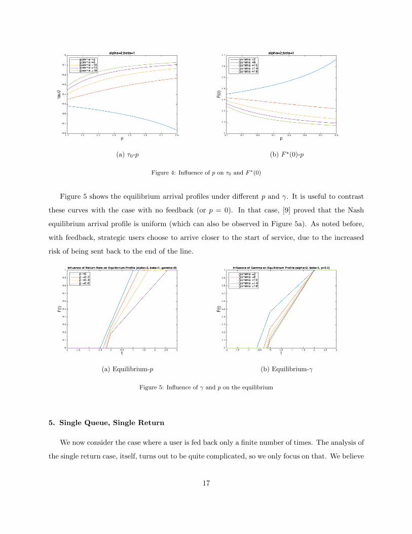
(a) τ0-p (b) F ?(0)-p

Figure 4: Influence of p on τ0 and F ?(0)

Figure 5 shows the equilibrium arrival profiles under different p and γ. It is useful to contrast

these curves with the case with no feedback (or p = 0). In that case, [9] proved that the Nash

equilibrium arrival profile is uniform (which can also be observed in Figure 5a). As noted before,

with feedback, strategic users choose to arrive closer to the start of service, due to the increased

risk of being sent back to the end of the line.

(a) Equilibrium-p (b) Equilibrium-γ

Figure 5: Influence of γ and p on the equilibrium

5. Single Queue, Single Return

We now consider the case where a user is fed back only a finite number of times. The analysis of

the single return case, itself, turns out to be quite complicated, so we only focus on that. We believe

17

that the generalization to the multiple, but finite, return case should be relatively straightforward

using the mathematical analysis we develop here, but we do not pursue this.

5.1. Individual Cost

The expected “risk” of being returned to the end of line after completing service for a user who

arrived at time t is G(t) = pR(t), where

R(t) =

1µQ(F (t)µ

), if t ≤ 0

1µQ(p(t−m(At)) + F (t)

µ

), if t > 0,

(21)

where m(·) is the Lebesgue measure and At is the set of time instances before t at which returning

users are served, as defined in (2). Thus the cost of arriving at time t is C(t) = (α+ β)w(t) + βt+

γpR(t), and w(t) is defined in (2).

The additional waiting time effected by the previous returns is much trickier to compute now

since the effective ‘return rate’ is time dependent. Essentially, a user who has returned once will not

return again, and consequently the effective return rate is less than or equal to pµ, in contrast to

the infinite return case. Intuitively, this phenomenon starts as soon as the first user to be fedback

receives her second service. Our first result establishes the existence of a Nash equilibrium arrival

profile when the queue length is piecewise linear.

Theorem 4. There exists a Nash Equilibrium such that the corresponding queue length function

Q is piecewise linear.

Proof. Suppose Q(t), t > 0 is linear, we conclude that R(t)w(t) = 1+p−F (0)

1+p for t > 0 using the geometric

argument aluded to in Figure 2. Then, the cost of arriving at time t is

C(t) = (α+ β) w(t) + βt+ γpR(t)

=

(γp

1 + p− F (0)

1 + p+ α+ β

)w(t) + βt,

where w(t) = µ−1Q(t)−min(0, t). Now, suppose t > 0, t+ δt ≤ 1 + p, and δt > 0. Then,

C(t) =

(γp

1 + p− F (0)

1 + p+ α+ β

)Q(t)

µ+ βt, and

C(t+ δt) =

(γp

1 + p− F (0)

1 + p+ α+ β

)Q(t+ δt)

µ+ β(t+ δt).

18

Since the arrival cost at equilibrium is constant in the arrival horizon, by setting C(t) = C(t+ δt)

we obtainQ(t+ δt)−Q(t)

δt=

−βµγp1+p−F (0)

1+p + α+ β=: k1.

Letting δt→ 0, it follows that the first order derivative of Q is constant for t > 0. Thus, it follows

that Q(t) = k1t+ b1 for t > 0, where b1 can be determined by solving the corresponding differential

equation and using the boundary condition Q1(τ1) = 0.

Next, suppose t < 0, t+ δt ≤ 0, and δt > 0. Then,

C(t) = (α+ β)w(t) + βt+ γpR(t)

=(α+ β)Q(t)

µ+ βt+ γpµ−1Q

(Q(t)

µ

)=

k1γpµ+ α+ β

µQ(t) + βt+ γpb1, and

C(t+ δt) =k1γpµ+ α+ β

µQ(t+ δt) + β(t+ δt) + γpb1.

Hence,Q(t+ δt)−Q(t)

δt=

µβ

k1γpµ+ α+ β=: k2,

implying that the first order derivative of Q(t) t ≤ 0 is a constant, and we have Q(t) = k2t + b2

where b2 can be determined by solving the differential equation with boundary condition Q(τ0) = 0.

Therefore, with such a piecewise linear Q(t), the cost is invariant over the arrival horizon [τ0, τ1].

The corresponding F (t) is the Nash equilibrium arrival profile.

Note that this result does not provide an expression for the equilibrium arrival profile F ?.

Based on the linearity of the queue length, one might conclude that F ?(t) is linear. However,

this intuition is, in fact, incorrect since the return ‘rate’ (defined as the fraction of all users who

might be fedback to the queue) is now time dependent. On the contrary, the return rate is af-

fected by the users who have already returned once - and they will never return again. We

next establish a description of the workload that formalizes this intuition. Recall that Ω :=

Set of all time instants where returning users are served andm : R+ → R+ the standard Lebesgue

measure.

Proposition 1. Let t0 = 0, and tk = tk−1 +Q(tk−1)

µ k ≥ 1 be the time point when users in the

19

queue at time epoch tk−1 are served. Denote At = x ∈ Ω : x ≤ t. Then, at equilibrium,

m(At0) = 0

m(Atk+1) = m(Atk) + p(tk − tk−1 − (m(Atk)−m(Atk−1

))) ∀k ≥ 1.

Proof. Since the server operates without idling at equilibrium the total time spent serving feedback

users is m(Ω) = µ−1p. Clearly, m(At) = 0 for t ≤ 0 and m(At0) = 0. Since t1 = µ−1Q(0) is the

first time epoch at which a feedback user receives her second service, we have m(At1) = 0.

From t1 to t2, the set of users receiving their second service is precisely those fedback between

t0 and t1. Since all the users arriving for the first time between t0 and t1 will have a chance to

return, it follows that m(At2) = m(At1) + p(t1 − t0).

From t2 to t3, the set of users being served for the second time is precisely those fedback between

t1 and t2. On the other hand the workload from users who will not return between t1 and t2 is

m(At2) − m(At1), implying that the total workload fedback is p(t2 − t1 − (m(At2) − m(At1))).

Hence m(At3) = m(At2) + p(t2 − t1 − (m(At2) −m(At1))). Continuing in this manner it follows

that m(Atk+1) = m(Atk) + p(tk − tk−1 − (m(Atk)−m(Atk−1

))) ∀k ≥ 1.

Now, the expected disutility of arriving at time t is

C(t) =

(α+β)Q(t)

µ − αt+ γpQ(

F (t)µ

)

µ , if t ≤ 0

(α+β)Q(t)µ + βt+ γp

Q(t+Q(t)µ

)

µ , if t > 0

(22)

where

Q(t) =

F (t), if t ≤ 0

F (t)− µt+ pµ(t−m(At)), if t > 0.

(23)

Our next result establishes the uniqueness of the equilibrium under a sufficient condition on the

parameters of the disutility.

Theorem 5. The Nash equilibrium is unique if α+βγp > 1.

First, consider the following lemma.

Lemma 4. Let an and bn be two sequences such that

c1an + bn + c2an+1 = 0, (24)

where b0 = 0, a0 = δ 6= 0, bn+1 =i=n∑i=0

ai. Then an does not converge to 0 if c1c2> 1.

20

Proof. Recursively expanding an, we obtain:

an+1 = −c1c2an −

1

c2bn

= (−c1c2

)n+1δ −n∑i=0

bic2

(−c1c2

)n−i

= (−c1c2

)n+1δ −n∑i=0

(−c1c2

)n−ii−1∑j=0

aj

= (−c1c2

)n+1δ − δ

c2

n−1∑j=0

aj

n∑i=j+1

(−c1c2

)n−i

= (−c1c2

)n+1δ − δn−1∑j=0

ajc1 + c2

(−c1c2

)n(

(−c2c1

)j+1 − (−c2c1

)n+1

).

Therefore,

an+1 − an = δ(−c1c2

)n(− c1c2− 1− 1

(c1 + c2)

(an−1(−

c2c1

)n − an−1(−c2c1

)n+1)

))= − δ

c2

((c1 + c2)(−

c1c2

)n +c2c1an−1

).

Suppose an → 0 as n→∞. i.e. ∀ε > 0, ∃N such that |an| < ε for ∀n > N , which implies

an+1 − an ≥ −δ

c2

((c1 + c2)(−

c1c2

)n +c2c1ε

).

It follows that

a2n − a2n−1 ≥ −δ

c2

(− (c1 + c2)(

c1c2

)2n−1 +c2c1ε

).

Next, let

N ′ =

⌈2−1log c1

c2

εc2(2 + δc1

)

δ(c1 + c2)

⌉,

so that

a2n − a2n−1 ≥ −δ

c2

(− (c1 + c2)(

c1c2

)2n−1 +c2c1ε

)> 2ε (25)

for all n > maxN,N ′. However, this implies either |a2n| > ε or |a2n−1| > ε. But, this contradicts

our assumption that |an| < ε, and by reductio the proof is complete.

Proof of Theorem 5. Suppose there are two different Nash equilibria F ?(t) and F ∗∗(t) with corre-

sponding queue length functions Q?(t) and Q∗∗(t). We describe the difference of the two equilibri-

ums by Q?(tx)−Q∗∗(tx) = δ > 0 and then argue by contradiction.

21

It is argued in theorem 2 that cost of the two equilibrium profiles are equal (i.e. C(τ?)) in

infinite return case. It is trivial that the argument also applies for single return case. We define

two time sequences as follows:

Ti(tx) =

tx, if i = 0

Ti−1(tx) + Q?(Ti−1(tx))µ , if i > 0.

(26)

T ′i (tx) =

tx, if i = 0

T ′i−1(tx) +Q∗∗(T ′i−1(tx))

µ , if i > 0.

(27)

Let C?(t) and C∗∗(t) be cost functions of F ? and F ∗∗ respectively. We have C?(Tn(t)) = C∗∗(T ′n(t)).

i.e.

α+ β

µ

(Q?(Tn(tx))−Q∗∗(T ′n(tx))

)+ β

(Tn(t)−T ′n(t)

)+γp

µ

(Q?(Tn+1(tx))−Q∗∗(T ′n+1(tx))

)= 0.

(28)

WLOG, set µ = 1 and let α+ββ = c?, γpβ = c∗∗, Q?(Tn(tx))−Q∗∗(T ′n(tx)) = an and Tn(t)−T ′n(t) = bn.

With this setting, it can be argued from equation (26) and (27) that bn+1 =i=n∑i=0

ai. Using notations

as defined above, equation (28) can be written as c?n + bn + c∗∗an+1 = 0.

Lemma 4 implies that an diverges if a0 = δ > 0 and c?

c∗∗ > 1, which contradicts with the claim

of Lemma 2 2. Hence, we obtain that a0 = 0. i.e. Q?(t)−Q∗∗(t) ≡ 0 for ∀t ∈ [τ0, τ1].

5.2. Equilibrium Arrival Profile

As noted before, the system does not idle in the support of the equilibrium arrival profile. Recall

that τ1 is the time of service termination. It is straightforward to argue that τ1 = µ−1(1 + p), since

µ−1p is the total feedback workload. The equilibrium cost of arriving at τ1 is C(τ1) = βτ1 =

βµ−1(1 + p). Since the Nash equilibrium condition in Definition 1 implies that the arrival cost is

constant in the support of the equilibrium arrival profile, it follows that

C(τ0) = C(τ1) =(1 + p)β

µ. (29)

From equation (22), (29) and the fact that F ?(τ0) = 0, we have τ0 = (µα)−1 (γpF ?(0)− β(1 + p)) .

2Note that while Lemma 2 is proved for the infinite-return case the same arguments hold for the single-return

case as well.

22

Now, assume that the equilibrium queue length Q? is piecewise linear. We know that Q?(0) =

F ?(0) and Q?(τ1) = 0. It follows that the slope of Q?(t) for t ≥ 0 equals

0− F ?(0)

τ1 − 0= −µF

?(0)

1 + p,

and the abscissa/intercept is F ?(0). On the other hand, if t < 0, we know that Q?(τ0) = 0 and

Q?(0−) = F ?(0), implying the slope is

F ?(0)− 0

0− τ0=

µαF ?(0)

β(1 + p)− γpF ?(0)

and the abscissa is F ?(0). Thus, it follows that

Q?(t) =

−µF ?(0)

1+p t+ F ?(0), if t > 0

µαF ?(0)β(1+p)−γpF ?(0) t+ F ?(0), if t ≤ 0.

(30)

Recall, from the proof of Theorem 3, that limδt→0Q?(t+δt)−Q?(t)

δt = −βµ(γp1+p−F

?(0)1+p + α+ β

)−1,

implying that

F ?(0) = (2pγ)−1

(α+ β + γp

p+ 1−

√(α+ β + γp

p+ 1)2 − 4γβp

(p+ 1)2

)(p+ 1)2. (31)

Now, recall that t0 = 0 and tk = tk−1+Q?(tk−1)

µ for k ≥ 1. The (piecewise) linearity of Q implies

thatti+2 − ti+1

ti+1 − ti=Q?(ti+1)

Q?(ti)=

1 + p− F ?(0)

1 + p.

Let q = (1 + p)−1(1 + p − F ?(0)), then Q?(ti) = F ?(0)qi and ti = µ−1∑j=i

j=1 F?(0)qj−1 for i > 0.

Furthermore, Proposition 1 showed that m(Ati+2) = m(Ati+1) + p(ti+1 − ti − (m(Ati+1 −m(Ati))),

implying thatq(m(Ati+2)−m(Ati+1)

)ti+2 − ti+1

= p

(1−

(m(Ati+1)−m(Ati))

ti+1 − ti

).

Denoting ki =(m(Ati+1 )−m(Ati ))

ti+1−ti (note that k0 = 0) we have, ki+1 = q−1p(1− ki) for i ≥ 1, so that

ki =∑i

j=1(−1)j−1(pq )j for i ≥ 1, and therefore

m(Ati+1) = m(Ati) + ki(ti+1 − ti) = m(Ati) + qit1ki.

Since m(At0) = 0, it follows that m(Ati+1) =∑i

j=1 qjt1kj .

23

By definition F ?(t) = Q?(t) + µt− pµ(t−m(At)), implying that

F ?(t) =

Q?(t) + µt− pµt, if t ∈ [t0, t1]

Q?(t) + µt− pµ(t−∑i

j=1 qjt1kj − ki(t− ti)), if t ∈ (ti+1, ti+2]

Q?(t), if t < 0.

(32)

Since

Q?(t) =

−µF ?(0)

1+p t+ F ?(0), if t > 0

µαF ?(0)β(1+p)−γpF ?(0) t+ F ?(0), if t ≤ 0,

(33)

we conclude that

F ?(t) =

−µF ?(0)1+p t+ F ?(0) + µt− pµt, if t ∈ (t0, t1]

− µF ?(0)

1 + pt+ F ?(0) + µt− pµ

[t−

i∑j=1

((1 + p− F ?(0)

1 + p

)j

t1

j∑k=1

(−1)k−1(

p(1 + p)

1 + p− F ?(0)

)k)−

i∑j=1

(−1)i−1(

p(1 + p)

1 + p− F ?(0)

)i(t− ti)

] if t ∈ (ti+1, ti+2]

µαF ?(0) (β(1 + p)− γpF ?(0))−1 t+ F ?(0), if t ≤ 0.

(34)

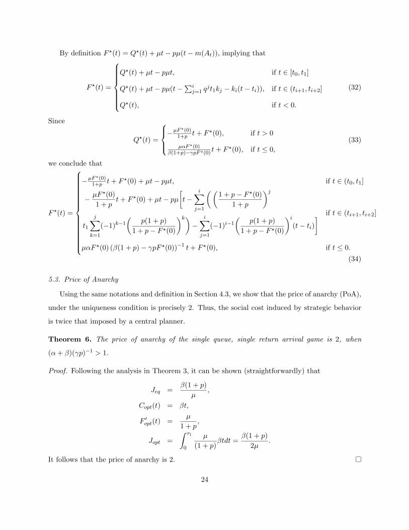
5.3. Price of Anarchy

Using the same notations and definition in Section 4.3, we show that the price of anarchy (PoA),

under the uniqueness condition is precisely 2. Thus, the social cost induced by strategic behavior

is twice that imposed by a central planner.

Theorem 6. The price of anarchy of the single queue, single return arrival game is 2, when

(α+ β)(γp)−1 > 1.

Proof. Following the analysis in Theorem 3, it can be shown (straightforwardly) that

Jeq =β(1 + p)

µ,

Copt(t) = βt,

F ′opt(t) =µ

1 + p,

Jopt =

∫ τ1

0

µ

(1 + p)βtdt =

β(1 + p)

2µ.

It follows that the price of anarchy is 2.

24

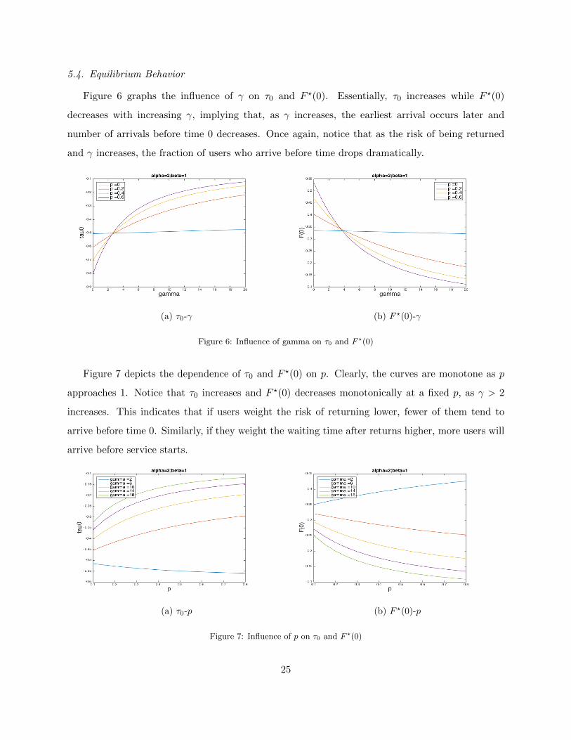
5.4. Equilibrium Behavior

Figure 6 graphs the influence of γ on τ0 and F ?(0). Essentially, τ0 increases while F ?(0)

decreases with increasing γ, implying that, as γ increases, the earliest arrival occurs later and

number of arrivals before time 0 decreases. Once again, notice that as the risk of being returned

and γ increases, the fraction of users who arrive before time drops dramatically.

(a) τ0-γ (b) F ?(0)-γ

Figure 6: Influence of gamma on τ0 and F ?(0)

Figure 7 depicts the dependence of τ0 and F ?(0) on p. Clearly, the curves are monotone as p

approaches 1. Notice that τ0 increases and F ?(0) decreases monotonically at a fixed p, as γ > 2

increases. This indicates that if users weight the risk of returning lower, fewer of them tend to

arrive before time 0. Similarly, if they weight the waiting time after returns higher, more users will

arrive before service starts.

(a) τ0-p (b) F ?(0)-p

Figure 7: Influence of p on τ0 and F ?(0)

25

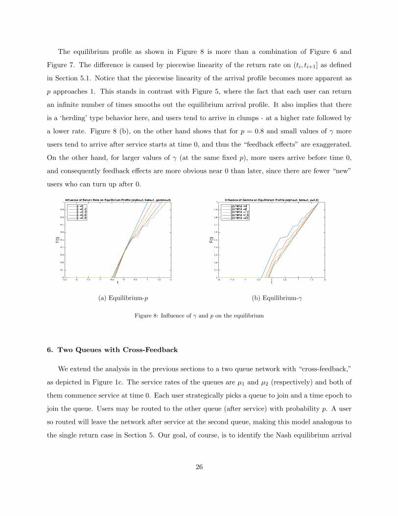
The equilibrium profile as shown in Figure 8 is more than a combination of Figure 6 and

Figure 7. The difference is caused by piecewise linearity of the return rate on (ti, ti+1] as defined

in Section 5.1. Notice that the piecewise linearity of the arrival profile becomes more apparent as

p approaches 1. This stands in contrast with Figure 5, where the fact that each user can return

an infinite number of times smooths out the equilibrium arrival profile. It also implies that there

is a ‘herding’ type behavior here, and users tend to arrive in clumps - at a higher rate followed by

a lower rate. Figure 8 (b), on the other hand shows that for p = 0.8 and small values of γ more

users tend to arrive after service starts at time 0, and thus the “feedback effects” are exaggerated.

On the other hand, for larger values of γ (at the same fixed p), more users arrive before time 0,

and consequently feedback effects are more obvious near 0 than later, since there are fewer “new”

users who can turn up after 0.

(a) Equilibrium-p (b) Equilibrium-γ

Figure 8: Influence of γ and p on the equilibrium

6. Two Queues with Cross-Feedback

We extend the analysis in the previous sections to a two queue network with “cross-feedback,”

as depicted in Figure 1c. The service rates of the queues are µ1 and µ2 (respectively) and both of

them commence service at time 0. Each user strategically picks a queue to join and a time epoch to

join the queue. Users may be routed to the other queue (after service) with probability p. A user

so routed will leave the network after service at the second queue, making this model analogous to

the single return case in Section 5. Our goal, of course, is to identify the Nash equilibrium arrival

26

profile (which now includes both routing and timing choices) when the cost of arriving at time t

follows (7).

6.1. Queueing Dynamics

Before discussing the Nash equilibrium computation, we briefly review the queue length dynam-

ics in the two queue network. Following the construction in Proposition 1, let t0 = Q1(0)µ1

, t′0 = Q2(0)µ2

and

tk+1 = t′k +Q1(t

′k)

µ1,

t′k+1 = tk +Q2(tk)

µ2.

Using the same induction as in the proof of Proposition 1, we obtain:

m(At0) = 0,

m(Atk+1) = m(Atk) + p(tk − tk−1 − (m(Atk)−m(Atk−1

))) ∀k ≥ 1,

and

m(A′t′0) = 0,

m(A′t′k+1) = m(A′t′k

) + p(t′k − t′k−1 − (m(A′t′k)−m(A′t′k−1

))) ∀k ≥ 1,

where the set At corresponds to the first queue and A′t is defined for the second queue. Note that

m(At) is linear on (tk, tk+1], while m(A′t) is linear on (t′k, t′k+1] for ∀k ≥ 0, k ∈ N. Recall that

Q1(t) and Q2(t) be queue lengths of the two queues. Let F ?1 (t) and F ?2 (t) be the corresponding

distribution functions. Then, unpacking (3)

Q1(t) =

F ?1 (t) if t ≤ 0,

F ?1 (t)− µt+ pµ(t−m(At)) if t > 0,

(35)

and

Q2(t) =

F ?2 (t), if t ≤ 0

F ?2 (t)− µt+ pµ(t−m(A′t)), if t > 0.

(36)

27

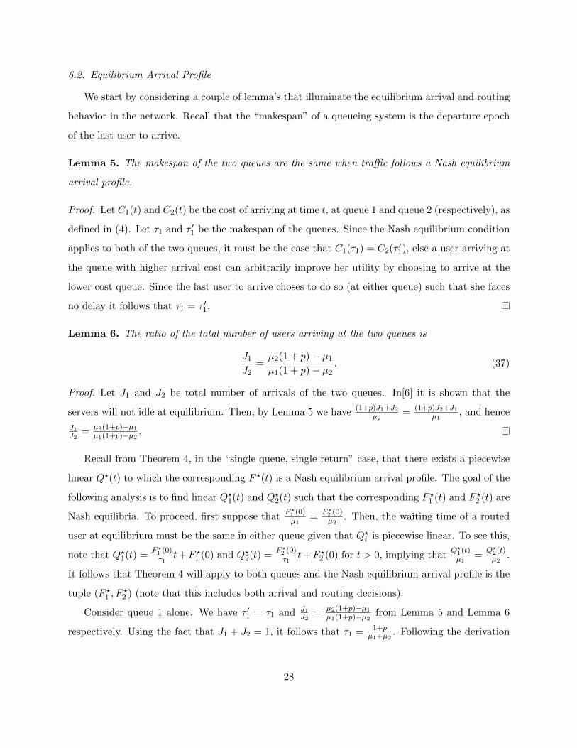
6.2. Equilibrium Arrival Profile

We start by considering a couple of lemma’s that illuminate the equilibrium arrival and routing

behavior in the network. Recall that the “makespan” of a queueing system is the departure epoch

of the last user to arrive.

Lemma 5. The makespan of the two queues are the same when traffic follows a Nash equilibrium

arrival profile.

Proof. Let C1(t) and C2(t) be the cost of arriving at time t, at queue 1 and queue 2 (respectively), as

defined in (4). Let τ1 and τ ′1 be the makespan of the queues. Since the Nash equilibrium condition

applies to both of the two queues, it must be the case that C1(τ1) = C2(τ′1), else a user arriving at

the queue with higher arrival cost can arbitrarily improve her utility by choosing to arrive at the

lower cost queue. Since the last user to arrive choses to do so (at either queue) such that she faces

no delay it follows that τ1 = τ ′1.

Lemma 6. The ratio of the total number of users arriving at the two queues is

J1J2

=µ2(1 + p)− µ1µ1(1 + p)− µ2

. (37)

Proof. Let J1 and J2 be total number of arrivals of the two queues. In[6] it is shown that the

servers will not idle at equilibrium. Then, by Lemma 5 we have (1+p)J1+J2µ2

= (1+p)J2+J1µ1

, and hence

J1J2

= µ2(1+p)−µ1µ1(1+p)−µ2 .

Recall from Theorem 4, in the “single queue, single return” case, that there exists a piecewise

linear Q?(t) to which the corresponding F ?(t) is a Nash equilibrium arrival profile. The goal of the

following analysis is to find linear Q?1(t) and Q?2(t) such that the corresponding F ?1 (t) and F ?2 (t) are

Nash equilibria. To proceed, first suppose thatF ?1 (0)µ1

=F ?2 (0)µ2

. Then, the waiting time of a routed

user at equilibrium must be the same in either queue given that Q?i is piecewise linear. To see this,

note that Q?1(t) =F ?1 (0)τ1

t+F ?1 (0) and Q?2(t) =F ?2 (0)τ1

t+F ?2 (0) for t > 0, implying thatQ?1(t)µ1

=Q?2(t)µ2

.

It follows that Theorem 4 will apply to both queues and the Nash equilibrium arrival profile is the

tuple (F ?1 , F?2 ) (note that this includes both arrival and routing decisions).

Consider queue 1 alone. We have τ ′1 = τ1 and J1J2

= µ2(1+p)−µ1µ1(1+p)−µ2 from Lemma 5 and Lemma 6

respectively. Using the fact that J1 + J2 = 1, it follows that τ1 = 1+pµ1+µ2

. Following the derivation

28

of cost function in Section 4.2, we have

C1(t) =

(α+β)Q?1(t)

µ1− αt+ γp

Q?1

(F?1 (t)

µ1

)µ1

if t ≤ 0,

(α+β)Q?1(t)µ1

+ βt+ γpQ?1

(t+

Q?1(t)

µ1

)µ1

if t > 0.

(38)

Notice that C1(τ1) = β(1+p)(µ1+µ2)

, so by setting C1(0) = C1(τ1) and solving for F ?1 (0) we obtain,

F ?1 (0) =

(2γp(µ1 + µ2)

µ21(1 + p)

)−1α+ β

µ1+γp

µ1−

√(α+ β

µ1+γp

µ1

)2

− 4

(γpβ

µ21

) . (39)

Let τ0 be such that F ?1 (t) = 0 for t ≤ τ0 and set C1(τ0) = C1(τ1), implying that τ0 =γpF ?1 (0)αµ1

−β(1+p)α(µ1+µ2)

. Therefore, following the computations in “Single Queue, Single Return,” we have

Q?1(t) =

−F ?1 (0)

τ0t+ F ?1 (0) if t ≤ 0,

−F ?1 (0)τ1

t+ F ?1 (0) if t > 0,

(40)

and

F ?1 (t) =

−F ?1 (0)τ1

t+ F ?1 (0) + µ1t− pµ2t if t ∈ (t0, t1],

− F ?1 (0)

τ1t+ F ?1 (0) + µ1t− pµ2

[t−

i∑j=1

((1 + p− F ?1 (0)

1 + p

)j

t1

j∑k=1

(−1)k−1(

p(1 + p)

1 + p− F ?1 (0)

)k)−

i∑j=1

(−1)i−1(

p(1 + p)

1 + p− F ?1 (0)

)i(t− ti)

] if t ∈ (ti+1, ti+2]

−F ?1 (0)τ0

t+ F ?1 (0) if t ≤ 0.

(41)

Now, by the previous construction, F ?2 (0) = F ?1 (0)µ2µ1 . Let τ ′0 be such that F ?2 (t) = 0 for t ≤ τ ′0,

then τ ′0 =γpF ?2 (0)αµ2

− β(1+p)α(µ1+µ2)

. Therefore, similarly,

Q?2(t) =

−F ?2 (0)

τ ′0t+ F ?2 (0) if t ≤ 0,

−F ?2 (0)τ1

t+ F ?2 (0) if t > 0,

(42)

29

and

F ?2 (t) =

−F ?2 (0)τ1

t+ F ?2 (0) + µ2t− pµ1t if t ∈ (t0, t1],

− F ?2 (0)

τ1t+ F ?2 (0) + µ2t− pµ1

[t−

i∑j=1

((1 + p− F ?2 (0)

1 + p

)j

t1

j∑k=1

(−1)k−1(

p(1 + p)

1 + p− F ?2 (0)

)k)−

i∑j=1

(−1)i−1(

p(1 + p)

1 + p− F ?2 (0)

)i(t− ti)

] if t ∈ (ti+1, ti+2]

−F ?2 (0)τ ′0

t+ F ?2 (0) if t ≤ 0.

(43)

Theorem 7. The Nash equilibrium is unique if α+βγp > 1 and

Q?1(t)µ1

=Q?2(t)µ2

.

Proof. It’s sufficient to show that Q?1 is unique since proof for Q?2 is identical. Suppose there exists

another Nash equilibrium such that the corresponding queue length function Q?′1 (tx) − Q?1(tx) =

δ > 0 for some tx in the support of the equilibrium arrival profile. Following the proof of Theorem

5 in Section 5.1, we obtain the equilibrium equation:

α+ β

µ1

(Q?1(Ti(t))−Q∗∗1 (T ′i (t))

)− β(Ti(t)− T ′i (t)) +

γp

µ2

(Q?2(Ti+1(t))−Q∗∗2 (T ′i+1(t))

)= 0. (44)

SinceQ?1(t)µ1

=Q?2(t)µ2

, equation (44) can be written as:

α+ β

µ1

(Q?1(Ti(t))−Q∗∗1 (T ′i (t))

)− β(Ti(t)− T ′i (t)) +

γp

µ1

(Q?1(Ti+1(t))−Q∗∗1 (T ′i+1(t))

)= 0. (45)

Let α+ββµ1

= c1,γpβµ1

= c2, Q?1(Tn(tx))−Q∗∗1 (T ′n(tx)) = an and Tn(t)− T ′n(t) = bn. Then the desired

result follows directly from lemma 4.

Figure 9 demonstrates the arrival profile of the Nash equilibrium as derived in equation (41)

and (43). We see that the increasing pattern of F ?i (t)(i = 1, 2) is the similar to that in figure

8. Notice, too, the ‘herding’ behavior where users choose to arrive in clumps of higher and lower

arrival ‘rates.’

7. Conclusion

Our goal in this paper was to study the effect of feedback routing on the Nash equilibrium arrival

timing and routing behavior of strategic users. As we demonstrate, the network architecture will

affect the Nash equilibrium profile. The infinite return and single return risk affects when users

30

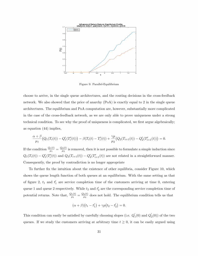
Figure 9: Parallel-Equilibrium

choose to arrive, in the single queue architectures, and the routing decisions in the cross-feedback

network. We also showed that the price of anarchy (PoA) is exactly equal to 2 in the single queue

architectures. The equilibrium and PoA computation are, however, substantially more complicated

in the case of the cross-feedback network, as we are only able to prove uniqueness under a strong

technical condition. To see why the proof of uniqueness is complicated, we first argue algebraically;

as equation (44) implies,

α+ β

µ1

(Q1(Ti(t))−Q′1(T ′i (t))

)− β(Ti(t)− T ′i (t)) +

γp

µ2

(Q2(Ti+1(t))−Q′2(T ′i+1(t))

)= 0.

If the condition Q1(t)µ1

= Q2(t)µ2

is removed, then it is not possible to formulate a simple induction since

Q1(Ti(t)) −Q′1(T ′i (t)) and Q2(Ti+1(t)) −Q′2(T ′i+1(t)) are not related in a straightforward manner.

Consequently, the proof by contradiction is no longer appropriate

To further fix the intuition about the existence of other equilibria, consider Figure 10, which

shows the queue length function of both queues at an equilibrium. With the same setting as that

of figure 2, t1 and t′1 are service completion time of the customers arriving at time 0, entering

queue 1 and queue 2 respectively. While t2 and t′2 are the corresponding service completion time of

potential returns. Note that, Q1(t)µ1

= Q2(t)µ2

does not hold. The equilibrium condition tells us that

(α+ β)(t1 − t′1

)+ γp

(t2 − t′2

)= 0.

This condition can easily be satisfied by carefully choosing slopes (i.e. Q′1(0) and Q

′2(0)) of the two

queues. If we study the customers arriving at arbitrary time t ≥ 0, it can be easily argued using

31

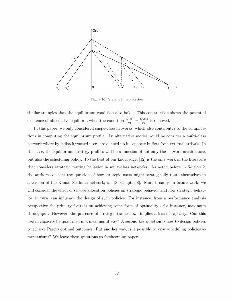
Figure 10: Graphic Interpretation

similar triangles that the equilibrium condition also holds. This construction shows the potential

existence of alternative equilibria when the condition Q1(t)µ1

= Q2(t)µ2

is removed.

In this paper, we only considered single-class networks, which also contributes to the complica-

tions in computing the equilibrium profile. An alternative model would be consider a multi-class

network where by fedback/routed users are queued up in separate buffers from external arrivals. In

this case, the equilibrium strategy profiles will be a function of not only the network architecture,

but also the scheduling policy. To the best of our knowledge, [12] is the only work in the literature

that considers strategic routing behavior in multi-class networks. As noted before in Section 2,

the authors consider the question of how strategic users might strategically route themselves in

a version of the Kumar-Seidman network; see [3, Chapter 8]. More broadly, in future work, we

will consider the effect of service allocation policies on strategic behavior and how strategic behav-

ior, in turn, can influence the design of such policies. For instance, from a performance analysis

perspective the primary focus is on achieving some form of optimality - for instance, maximum

throughput. However, the presence of strategic traffic flows implies a loss of capacity. Can this

loss in capacity be quantified in a meaningful way? A second key question is how to design policies

to achieve Pareto optimal outcomes. Put another way, is it possible to view scheduling policies as

mechanisms? We leave these questions to forthcoming papers.

32

References

[1] Alessandro Arlotto, Andrew E Frazelle, and Yehua Wei. Strategic open routing in queueing

networks. Available at SSRN 2589258, 2015.

[2] Priv-Doz Dr D Braess. Uber ein paradoxon aus der verkehrsplanung. Unternehmensforschung,

12(1):258–268, 1968.

[3] Hong Chen and David D Yao. Fundamentals of queueing networks: Performance, asymptotics,

and optimization, volume 46. Springer Science and Business Media, 2013.

[4] Amihai Glazer and Refael Hassin. ?/m/1: On the equilibrium distribution of customer arrivals.

Eur. J. Oper. Res., 13(2):146–150, 1983.

[5] Refael Hassin and Moshe Haviv. To queue or not to queue: Equilibrium behavior in queueing

systems, volume 59. Springer Science and Business Media, 2003.

[6] Harsha Honnappa and Rahul Jain. Strategic arrivals into queueing networks: the network

concert queueing game. Oper. Res., 63(1):247–259, 2015.

[7] Harsha Honnappa and Rahul Jain. Transitory queueing networks. In Preparation, 2016.

[8] Rahul Jain, Sandeep Juneja, and Nahum Shimkin. The concert queueing game: to wait or to

be late. Disc. Event Dyn. Syst., 21(1):103–138, 2011.

[9] Sandeep Juneja and Rahul Jain. The concert/cafeteria queueing problem: a game of arrivals. In

Proceedings of the Fourth International ICST Conference on Performance Evaluation Method-

ologies and Tools, page 59. ICST (Institute for Computer Sciences, Social-Informatics and

Telecommunications Engineering), 2009.

[10] Sandeep Juneja and Nahum Shimkin. The concert queueing game: strategic arrivals with

waiting and tardiness costs. Queueing Syst., 74(4):369–402, 2013.

[11] Pinhas Naor. The regulation of queue size by levying tolls. Econometrica: J. Econometric

Soc., pages 15–24, 1969.

[12] Ali K Parlakturk and Sunil Kumar. Self-interested routing in queueing networks. Management

Sci., 50(7):949–966, 2004.

33