application of hadamard transform ion mobility mass

APPLICATION OF HADAMARD TRANSFORM ION MOBILITY MASS

SPECTROMETRY TO GLOBAL METABOLOMICS

By

XING ZHANG

A dissertation submitted in partial fulfillment of the requirements for the degree of

DOCTOR OF PHILOSOPHY

WASHINGTON STATE UNIVERSITY Department of Chemistry

AUGUST 2014

© Copyright by XING ZHANG, 2014 All Rights Reserved

ii

To the Faculty of Washington State University: The members of the Committee appointed to examine the dissertation of Xing Zhang find it satisfactory and recommend that it be accepted.

Herbert H. Hill, Ph.D., Chair

William F. Siems, Ph.D.

Peter T. A. Reilly, Ph.D.

Brian H. Clowers, Ph.D.

Nairanjana Dasgupta, Ph.D.

iii

ACKNOWLEDGEMENTS

I would like to first express my gratitude to my advisor Dr. Herbert. H. Hill, for accepting me

to the big family of Hill’s group, and for his continual support and guidance throughout the

past five years. I am very lucky to have a great advisor who gives me encouragement all the

time. I would also want to thank Dr. William F. Siems for his advice and help both in lab and

in life. He brings ideas, laugh, and stories that can always cheer me up. I wish to

acknowledge the contributions of Dr. Peter Reilly and Dr. Brian Clowers, for their valuable

time and expertise in Chemistry. I also want to thank Dr. Nairanjana Dasgupta for her

guidance and help in Statistics.

A special thanks to Dr. Kimberly Kaplan for her exceptional help at the beginning of my

graduate career. And I also want to thank all past and present group members, who made my

graduate school life happy and cheerful. I would like to acknowledge our collaborators Dr.

Richard Knochenmuss, Dr. Stephan Graf, Dr. James Schenk, Dr. George Stoica, Dr. Barbara

Sorg, and Dr. Patrick Tso, for their great support.

None of this work would have been possible without the constant support from my parents

and my dear husband Rui Zhu, whose love and support made the life in Pullman sweet and

joyful. Finally, I would like to thank the Department of Chemistry for offering me the chance

to come to USA and pursue my PhD. It has been a wonderful journey!

iv

APPLICATION OF HADAMARD TRANSFORM ION MOBILITY MASS

SPECTROMETRY TO GLOBAL METABOLOMICS

Abstract

by Xing Zhang, Ph.D. Washington State University

August 2014

Chair: Herbert H. Hill, Jr.

Conventional Ion mobility mass spectrometry (IMMS) provides rapid separation and

detection of complex mixtures. It is merging as a powerful analytical platform for the field of

metabolomics but is limited in throughput. Global metabolomics aims at comprehensive

measurement for all metabolites and presents challenges in analytical technique. The work

describe herein evaluates the capability of hadamard transform ion mobility mass

spectrometry (HT-IMMS) for comprehensive metabolomics analysis with high throughput

and high resolving power. The work also presents a number of applications of global

metabolomics regarding to biological systems including human blood, rat brain tissue and

mice plasma.

HT-IMMS has been developed by superimposing a Hadamard transform sequence on the ion

gate. This development provides a 50% duty cycle while retaining high IMS resolving power.

v

Coupling rapid chromatographic separation prior to HT-IMMS enables the detection of more

metabolite features compared to conventional direct infusion IMMS.

Global metabolomic applications of HT-IMMS were extended in this work by developing

general procedure for sample analysis, metabolite identification, data processing and

statistical analysis. The major findings from this work include: 1) HPLC couple with

HT-IMMS provides comprehensive metabolomics analysis within 2 - 3 minutes; 2) ambient

pressure IMMS has high resolving power and allows isomeric separations, providing accurate

assessment of critical biomarkers without the interference of their isomers; 3) the structural

information generated from IMMS analysis complements the MS detection and helps

metabolite identifications; 4) principle component analysis yields pattern recognition that can

reveal the differences between different metabolic states; 5) biomarkers selection requires the

combination of multivariate analysis and univariate analysis; 6) IMMS data pre-processing,

including normalization and the evaluation of censored data, improves statistical analysis.

HT-IMMS is a natural fit for analyzing complex mixtures.

vi

TABLE OF CONTENTS Page

ACKNOWLEDGEMENTS ..................................................................................................... iii

ABSTRACT .............................................................................................................................. iv

TABLE OF CONTENTS .......................................................................................................... vi

LIST OF TABLES .................................................................................................................... ix

LIST OF FIGURES .................................................................................................................. xi

Chapter 1 .................................................................................................................................. 1

Introduction ................................................................................................................................ 1

1.1 Ion Mobility Spectrometry ............................................................................................ 1

1.2 Types of IMS Devices .................................................................................................. 9

1.3 Ion Mobility Mass Spectrometry: Multidimensional Separation ............................... 13

1.4 Application of IMMS to Complex Mixture Analyses ................................................ 18

1.5 Future Improvements .................................................................................................. 21

1.6 Specific Aims .............................................................................................................. 22

1.7 Attribution ................................................................................................................... 24

Chapter 2 ................................................................................................................................ 30

Metabolic Analysis of Striatum Tissues from Parkinson’s Disease-like Rats by Electrospray

Ionization Ion Mobility Mass Spectrometry ............................................................................ 30

2.1 Introduction ................................................................................................................. 32

2.2 Experimental Design ................................................................................................... 36

vii

2.3 Results and Discussion ............................................................................................... 42

2.4 Conclusions ................................................................................................................. 47

Chapter 3 ................................................................................................................................ 59

Evaluation of Hadamard Transform Atmospheric Pressure Ion Mobility Time-of-Flight Mass

Spectrometry (HT-APIMS-TOFMS) for Complex Mixture Analysis ..................................... 59

3.1 Introduction ................................................................................................................. 60

3.2 Theoretical Background .............................................................................................. 65

3.3 Experimental Section .................................................................................................. 66

3.4 Results and Discussion ............................................................................................... 71

3.5 Conclusions ................................................................................................................. 78

3.6 Supplementary Materials ............................................................................................ 90

Chapter 4 ................................................................................................................................ 91

Strategies for Metabolite Identification in Human Blood Metabolome using Electrospray

Ionization Hadamard Transform Ion Mobility Time-of-Flight Mass Spectrometry ............... 91

4.1 Introduction ................................................................................................................. 93

4.2 Experimental Section .................................................................................................. 96

4.3 Results and Discussion ............................................................................................. 101

4.4 Conclusions ............................................................................................................... 107

Chapter 5 .............................................................................................................................. 124

Neuronal Metabolomics by Ion Mobility Mass Spectrometry in Cocaine Self-administering

Rats after Early and Late Withdrawal .................................................................................... 124

viii

5.1 Introduction ............................................................................................................... 125

5.2 Experimental Design ................................................................................................. 128


5.4 Conclusions ............................................................................................................... 140

Chapter 6 .............................................................................................................................. 157

Metabolomics of Plasma Fluids from Apolipoprotein AV Knockout Mice by Hadamard

Transform Ambient Pressure Ion Mobility Time-of-Flight Mass Spectrometry ................... 157

6.1 Introduction ............................................................................................................... 159

6.2 Experimental Section ................................................................................................ 163


6.4 Conclusions ............................................................................................................... 174

Chapter 7 .............................................................................................................................. 188

Conclusions ............................................................................................................................ 188

Appendix ............................................................................................................................... 194

ix

LIST OF TABLES Page

Chapter 2

Table 2.1. Number of reproducible ions detected in each sample for principal component

analysis. .................................................................................................................................... 51

Table 2.2. Major ion peaks (ion counts > 100) detected in PD-like samples, BD-IV and SD

healthy controls. m/z ranges between 200 and 900. ................................................................ 52

Table 2.3. Tentative metabolite identifications based on exact m/z using the Human

Metabolome Database, including molecular formula and adducts. ......................................... 53

Chapter 3

Table 3.1 A table of the m/z, drift time, reduced mobility (K0) value and calibration curves

for each metabolite ion. Obtained from the analysis of metabolite standard mixture solutions.

.................................................................................................................................................. 82

Table 3.2 A summary of the absence/presence of six metabolite ions during the analysis of

standard mixture solutions in both HT-IMMS mode and pulsed-IMMS mode. ...................... 83

Chapter 4

Table 4.1 Metabolite identification of 185 major metabolite features detected by

HT-IMtofMS. Measured m/z, drift time and K0 are included. .............................................. 111

Table 4.2 Isotopic ratio analysis results. ................................................................................ 116

Table 4.3 Isomer/isobar separation and analysis results. ....................................................... 116

Table 4.4 Mobility-mass correlation trend lines. ................................................................... 117

x

Chapter 5

Table 5.1 Sample details and cocaine self-administration results including the total number of

active lever presses and the total number of rewards accumulated. ...................................... 145

Table 5.2 Sample list with number of reproducible metabolite features (counts>50) detected

by HT-IMMS in each sample group. ..................................................................................... 145

Table 5.3 Lists of potential biomarkers generated from loadings plots and univariate analysis.

Information includes measured m/z, p-value of t-test, up/down regulation caused by cocaine

administration, adduct form, and identified metabolite name, is listed in table. ................... 146

Chapter 6

Table 6.1 Summary of experimental details. ......................................................................... 178

Table 6.2 Summary of the identifications of the first 40 major metabolite features detected in

all 11 samples. The exact m/z and K0 (cm2V-1s-1) were measured in IMMS analysis, and the

identifications were matched with existing databases. .......................................................... 179

xi

LIST OF FIGURES Page

Chapter 1

Figure 1.1 Illustration of ions separation in flat electrodes DIMS. ……………………….11

Figure 1.2 Schematic picture of electrospray ion mobility time-of-flight mass spectrometer,

with major components: electrospray, DT IMS, IMMS interface and reflectron time-of-flight

mass spectrometer……………………………………………………………………………14

Figure 1.3 IMMS 2-D plot showing fragmentation pattern of [Dopamine + H]+………….15

Chapter 2

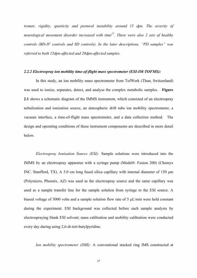
Figure 2.1 Schematic diagram of an electrospray ion mobility time-of-flight mass

spectrometer. ............................................................................................................................ 53

Figure 2.2 Multidimensional IMMS spectra of (a) the electrospray background, (b) SD

healthy control metabolome from striatal tissue, and (c) an expanded view of (b). ................ 54

Figure 2.3 MS and IMS spectra for BD-IV and SD healthy control striatal metabolomes are

shown in (a) and (b); MS and IMS spectra for PD affected 20 dpn and 15 dpn strital

metabolomes are shown in (c) and (d).. ................................................................................... 55

Figure 2.4 Principle component analysis results for all reproducible metabolite ions.. .......... 56

Figure 2.5 Selected m/z 154 mobility spectrums abstracted from the overall IMMS spectrums

for ESI background, BD-IV healthy control striatal metabolomes and BD-IV 20dpn affected

striatal metabolomes. ............................................................................................................... 57

Figure 2.6 Scheme of proposed dopamine and 2-(2,4-dihydroxyphenyl) ethylamine path. .... 58

xii

Chapter 3

Figure 3.1 Schematic diagram of the prototype: Electrospray ionization Hadamard transform

atmospheric pressure ion mobility time-of-flight mass spectrometer.. .................................... 84

Figure 3.2 IMMS 3-dimensional spectra of NIST SRM 1950 sample. ................................... 85

Figure 3.3 Twelve calibration curves of the six metabolite ion species under HT-IMMS mode

and pulsed-IMMS mode.. ........................................................................................................ 86

Figure 3.4 IMS spectra of NIST SRM 1950 sample obtained in pulsed-IMMS mode,

HT-IMMS mode, and from Synapt G2 TWIMMS system. ..................................................... 87

Figure 3.5 Comparison of mobility traces of the MS peak m/z 317.12, in pulsed-IMMS mode

(upper) and HT-IMMS mode (lower).. .................................................................................... 88

Figure 3.6 (a) and (b) are the 3-D IMMS-Intensity plots of striatum tissue extract fluid

analyzed by HPLC coupled HT-IMMS and direct infuse HT-IMMS, respectively ................ 89

Figure 3.7 A portion of a typical HT code sequence (top trace), along with multiplexed data

(middle trace) and decoded spectrum (down trace). ................................................................ 90

Chapter 4

Figure 4.1 (a) Schematic diagram of electrospray ionization hadamard transform atmospheric

pressure ion mobility time-of-flight mass spectrometer; (b) major metabolites detected in

human blood metabolome; (c) major metabolites detected in NIST SRM 1950 ................... 118

Figure 4.2 Global metabolomics results from HT-IMtofMS analysis. .................................. 119

Figure 4.3 An example of accurate isotopic ratio analysis. ................................................... 120

Figure 4.4 An example of isomer/isobar separation.. ............................................................ 121

xiii

Figure 4.5 IMMS two-dimensional spectrum of hemoglobin with charge states from +13 to

+17. ........................................................................................................................................ 122

Figure 4.6 IMMS two-dimensional spectrum illustrating the metabolomes of human blood,

with six trend lines identified for different compound classifications. .................................. 123

Chapter 5

Figure 5.1 Schematic diagram electrospray hadamard transform ion mobility time-of-flight

mass spectrometer (HT-IMMS) coupled with HPLC ............................................................ 150

Figure 5.2 IMMS 2-D spectrum of the metabolomes of striatal tissue is displayed in (a). IMS

spectra illustrating the global metabolomes of PFC samples obtained from saline treatment

and cocaine treatment are shown in (b) ................................................................................. 151

Figure 5.3 PCA score plots of six comparisons ..................................................................... 153

Figure 5.4 Dysregulation of creatine and creatinine .............................................................. 154

Figure 5.5 Intensity profiles of GHS, showing its dysregultaion. ......................................... 155

Figure 5.6 Dysregulation of adenosine in STR/PFC/NAC after 1 day withdrawal and after 3

wks withdrawal. ..................................................................................................................... 156

Chapter 6

Figure 6.1 (a) Schematic diagram of electrospray ionization coupled with hadamard

transform ambient pressure ion mobility time-of-flight mass spectrometry. (b) Illustrative

IMMS 3D spectrum of a plasma sample ................................................................................ 181

Figure 6.2 Representative mass spectra (top) and ion mobility spectra (bottom) for four

different groups of samples, including plasma fluids from apoAV KO mice fasted for 5 hrs,

xiv

WT mice fasted for 5 hrs, apoAV KO mice ad lib fed and WT mice ad lib fed. ................. 182

Figure 6.3 PCA results including score plot (top) and loadings plot (bottom).. .................... 184

Figure 6.4 Specific metabolic alternations for lysophospholipid class of metabolites. ......... 185

Figure 6.5 Intensity profiles for glucose (a) and MG (18:0) (b) for four groups of samples. 186

Figure 6.6 Selected-mass ion mobility spectra for monosaccharide ion (m/z = 203.06). ..... 187

1

Chapter 1

Introduction

1.1 Ion Mobility Spectrometry

Ion mobility spectrometry (IMS)1 is an analytical separation technique that separates

gas-phase ions based on their size-to-charge ratio and ion-neutral interactions as they travel

through a drift tube filled with a drift gas. Separation in IMS occurs rapidly in millisecond

with high resolving power2. As an efficient separation with low detection limits, IMS is

applied in separating and detecting illicit drugs3,4, chemical warfare agents5 explosives

detection6, and biomolecules. The advent of soft ionization sources such as electrospray

(ESI)7 and matrix assisted laser desorption ionization (MALDI)8 have extended IMS

application to not only vapor samples, but also aqueous and solid phase samples. In recent

years, IMS has shown great potential for separating complex mixtures, including

pharmaceutical drugs9, biomolecules analysis10, metabolomics11, and proteomics12.

1.1.1 History

Ion mobility spectrometry was first introduced as an analytical technique known as

Plasma Chromatography (PC)13, which produced plasmagrams for ultratrace analysis of

organic compounds. The original PC tube consisted of four parts: 63Ni foil reactor complex to

generate charged particles; ion-injection grid to inject a pulse of ions; ion-drift tube for ion

separation and electrometer as the detector. The drifting action of the charged particles was

initially analogous to that of a time-of-flight mass spectrometer and the drift time was

analogous to the retention time in chromatography. PC showed potential of being a practical

2

and rapid analytical separation technique with very low detection limits, and those properties

made it attractive to military and security use for detecting explosives and chemical warfare

agents. To date, IMS is still a popular choice for security and military applications14. The

performance of IMS device has been improved in both industrial and academic laboratories

on IMS over the past few decades.

1.1.2 Theoretical Background

In the classical case, IMS separates ions based on their mobility through a drift tube in

which an electrostatic field propels the ions through the tube filled with a buffer gas. After

entering the drift tube through an ion gate/pulser, ions are accelerated in the electric field and

decelerated by the collisions with the buffer gas until they reach a constant ion velocity (vd),

which is proportional to the electric field (E). The mobility (K) of an ion is then characterized

as the ratio of its ion velocity to electric field, as shown in Equation 1.

! = !!! = !!

!!! !!!!!!!!!"#$%&'(!1

Where E is the electric field (volts/cm), V (volts) is the voltage drop across the drift tube with

length L (cm), td is the time an ion takes to migrate through the drift tube.

Fundamental information about ionic size under specific conditions can be derived

from mobility measurements. Revercomb and Mason et al. have given the relationship

between ion mobility and collision cross section (Ω) during the collision processes15, as

shown in Equation 2.

! = 3!16!

2!!!!

!/! ! +!!"

!/! 1Ω

!!!!!!!!!!!!"#$%&'(!2

3

Where q is the charge on an electron, N is the number density of the drift gas, kb is

Boltzmann’s constant, T is the temperature, M is the mass of the drift gas and m is the mass

of the ion.

Since IMS devices are operated at a variety of temperatures and that ambient pressure

also changes among geographical regions, and ion’s mobility is different for different

operating parameters. However, the reduced mobility constant (K0) for an ion species remains

constant for a given drift gas after standardized to standard temperature and pressure, as

shown in Equation 3. Thus K0 allows mobility comparisons among laboratories1,16.

!! =!!!!!×

273.15! × !

760 !!!!!!!!!!!!!"#$%&'(!3

1.1.3 IMS Figure of Merits

Resolving power and the number of theoretical plates:

As one of the most important factors for analytical separation techniques, resolving

power (Rp) is the parameter for quantifying the separation. It is commonly defined in terms of

single-peak-based equation, as

!! =!!!! !!!!!!!!!!!!!!!"#$%&'(!4

Where td is the drift time of the ion of interest and wh is the peak width measured at

half-height. As shown in this equation, the resolving power can be increased with narrower

peak width.

The study on peak width in IMS started in 1970’s, researchers first developed an

expression for peak width in IMS using several assumptions15. The first assumption was that

4

the peak shape in IMS is primarily dependent on two factors, which are initial gate pulse

width of the ion gate and the broadening due to diffusion. A pack of ions, after entering the

drift region, will experience diffusional broadening as it travels in the IMS tube. The

second assumption is that the initial ion pack is Gaussian in shape. Thus the final peak width

at half height can be expressed as Equation 5.

!! = !!! + !!"##!!!!!!!!!!!!!!!!!"#$%&'(!5

Where wh is the final peak width at half-height, tg is the initial ion pulse width, tdiff is the

width at half-height of an ion peak which is produced by an infinitely narrow gate pulse.

The diffusion term in Equation 6 was further extended based on the definition of

Brownian diffusion coefficient and Nernst-Einstein Equation, giving the following

expression in for the final peak width at half-height.

!! = !!! +16!!!"#2!"# !!!!!!!!!!!!!"#$%&'(!6

Where kb is the Boltzmann’s constant, T is the temperature, V is the voltage drop on the drift

tube, e is te charge on an electron, z is the number of charges on the ion, and td is the drift

time of the ion. Therefore, the resolving power17 can be written as the following equation:

!! =!!

!!! + 16!"#$2!"# !!!

!!!!!!!!!!!"#$%&'(!7

As shown in Equation 7, in order to increase the resolving power, one must increase

the voltage applied across the IMS, decrease the temperature, or decrease the initial gate

pulse width.

5

In chromatography, another measurement of separation capability is the theoretical

number of plates (N):

! = 16 !!!

!!!!!!!!!!!!!!!"#$%&'(!8

Where tr as retention time, w as the peak width at the base. N can be calculated in IMS with

an easy substitution of retention time with drift time. For a drift time ion mobility

spectrometer device with gate pulse width at 0.2 milliseconds and a drift time of 20

milliseconds, and operation at typical instrumental parameters (temperature at 473 K and

8000 V voltage drop across the tube), the predicting resolving power and number of plate

would be approximately 23,800.

Resolution, separation factor (α) and selectivity:

Resolution in chromatography is another representation of the efficiency of separation,

and in IMS, it is expressed by the commonly used two-peak definition. As shown in Equation

9:

! = !!! − !!!!! + !! 2

!!!!!!!!!!!!!!"#$%&'(!9

Where td1 is the drift time of the ion that drifts faster and td2 is the drift time of the ion that

drifts slower, w is the peak width at the base.

The separation factor (α) in IMS is defined as18 the Equation 10:

! = !!!!!! =

!!"!!" !!!!!!!!!!!!!!"#$%&'(!10

Similar as in chromatography, one would prefer higher α value and any α value of 1 indicates

that the two compounds cannot be separated. Different from chromatography, capacity factor

6

(k’) is very large in IMS. In the definition of capacity factor (k’=(td-t0)/t0), t0 is the time it

takes for an ion to drift down to the drift tube without interaction with the drift gas and it is

negligible when compared to an ion’s drift time in atmospheric pressure condition. The large

capacity factor indicates that in IMS the theoretical number of plates is very close to the

effective number of theoretical plates.

Unlike in chromatography, where the separation factor can be altered by optimizing

mobile/stationary phase, there are only limited factors can be changed in IMS. Several

methods of altering α were previously reported18-20. One method described by M. Tabrizchi et

al. differentiated the declustering/dehydration rates of the analytes by changing temperature;

another idea for altering α was by changing the polarizability and mass of the drift gas on

drift time ion mobility spectrometer, or alternating the composite of drift gas by adding

modifiers21. Studies showed the separation effects of several different drift gases on

structurally similar classes of compounds22,23, and the results showed that alteration of drift

gas changed the drift times of ions, however, the percentages of change were different from

one ion to another, hence the separation factor was altered. It was demonstrated that

separation factor is largely dependent on the polarizability of the drift gas, and optimal

separation can be achieved by optimizing the drift gas.

Analysis speed and sensitivity:

Another attribute of IMS is the rapid analysis time. Each ion mobility separation can

be achieved within 20 – 100 milliseconds. Thus, even through it is common to average

several of these separations for a single analysis; IMS has shortened the analysis time to a

few minutes. High sensitivity in detection also makes it suitable for quantifying trace level

concentrations. The limit of detection (LOD) of IMS is usually below microgram (µg) or

7

even nanogram (ng).

1.1.4 IMS Fundamental Separation Mechanism

Different from chromatography, IMS provides a piece of “hard” information called

collision cross section (Ω)24. Ω is directly related to the ionic structure; therefore, it is where

the ion mobility separation originates. At a given charge state, smaller ions encounter fewer

ion-neutral collisions compared with bigger ions. Although obtaining Ω information is

restricted to drift tube IMS, it is applicable to other types of IMS devices with calibration.

As shown in Equation 11, the average collision cross section can be predicted from

the drift time data after a simple rearrangement of Equation 2. And the obtained Ω can then

be correlated with the gas-phase ion conformation and be a fairly accurate estimate of the

ion’s size25.

Ω = 3!"16!

2!!"#

!/! !"!!!

!273.15

760! !!!!!!!!!!!"#$%&'(!11

Where these parameters include the charge of the ion (z), the drift gas number density (N),

Boltzmann’s constant (k), temperature (T), pressure of the drift gas (P), the voltage drop

across the drift tube (V), drift time (td), length of the drift tube (L), and reduced mass of the

ion-neutral collision pair µ, (µ = mM/(m+M). m and M are the ion and neutral masses,

respectively). In cases where temperature, pressure and gas phase conditions (number density

and gas purity) cannot be measured accurately, calibration procedure using ions with known

Ω is preferred26.

Collision cross section is particularly important with regard to the separation of

8

isomeric compounds27. Isomeric compounds cannot be separated by mass spectrometry,

although they have minor difference in their collision cross sections due to structural

differences; their mass is the same. With the high resolving power of IMS, separation of

isomers can be achieved. The ability to determine collision cross sections and to separate

isomers has assigned IMS enormous potential for the analysis of complex mixtures. When

coupled with MS, conformation information can be obtained. Use of collision cross sections

has been widely applied in proteomics, metabolomics and lipidomics28,29.

The above figure of merits has enabled IMS for complex sample analysis. Efficient

separations can be achieved because of the high resolving power of IMS; the milliseconds

separation in IMS makes it the top choice for degradable complex biological samples and

organic reaction monitoring; the collision cross section information provided by IMS can be

used for class identification of unknown components in complex samples.

9

1.2 Types of IMS Devices

The IMS technique has been improved for decades to provide customized applications.

IMS devices can now be operated under a wide temperature/pressure range using different

electric field conditions. Each type of IMS device has unique advances and properties,

enabling many analytical applications.

1.2.1 Ambient Pressure Drift-Time IMS (DTIMS)

DTIMS employs a simple and conventional design consisting of a stacked series of

metal ring electrodes isolated by ceramic ring insulations but electrically connected using a

resistor chain. This design creates a smooth electric field, driving ions to transmit through the

drift tube. Ion gate, buffer gas and detector are included to complete an IMS device. More

details about the fundamental theory were discussed in the previous section. Other materials

including resistive glass and polymer materials have been assessed for replacing the

conventional metal and ceramic ring components.

Most DTIMS devices operate under ambient pressure to 1) avoid the necessity of

vacuum pumping; 2) provide enough ion-neutral collisions using a miniature size drift tube.

Ambient pressure DTIMS can often achieves high resolving power (>100) separation in

millisecond time scale. Early DTIMS devices typically have a low duty cycle in which only

about 1% of the ion current is used for detection, however, this situation has improved in

recent years by implementing multiplexing methods30,31, in which the duty cycle can be

increased up to about 50%.

1.2.2 Low Pressure Drift-Time IMS

Low pressure DTIMS has been widely used in the analysis of biomolecules. It enables

10

easy coupling with mass spectrometer without complicated pressure interface, therefore, gain

better sensitivity when compared with ambient pressure DTIMS. With the recent

development of ion funnel trap (IFT) technique32,33, low pressure DTIMS is reported with

LODs of picomoles. However, limited Rp of low-pressure IMS systems is inevitable unless

extremely long drift tubes are employed.

1.2.3 Differential Mobility spectrometry (DMS)

Differential ion mobility spectrometry is also called high field asymmetric waveform

ion mobility spectrometry (FAIMS)34. The basic difference between DMS and DTIMS is that

instead of using electrostatic fields, DMS employs a periodic asymmetric electric field in a

gap between two electrodes and in a direction perpendicular to the buffer gas flow. Ions in

DMS will experience alternately strong and weak orthogonal electric fields (or E/N). If the

mobility of an ion swarm is greater in one direction than in the other, the ion will have an

unstable path through the spectrometer and neutralize on the side of the spectrometer. As the

drift gas pushes the ions through the spectrometer, a compensation voltage can be used to

offset the ion swarm’s trajectory toward the side of the gap and enables the ions to migrate

through the spectrometer and be collected and detected on the terminal electrode. The

mobility difference (ΔK) of a given ion species under high and electric fields is expressed by

the compensation field, because only ions with a certain ΔK can be successfully transported

under the present condition. The separation procedure of DMS is shown in Figure 1.1. By

scanning a range of compensation voltages, ions with different ΔK can be transported

through the spectrometer separately.

11

Figure 1.1: Illustration of ions separation in flat electrodes DIMS.

Unlike DTIMS, DMS has an advantage of low-cost construction since most of the

devices work under ambient pressure and are designed in a smaller scale (a few square

centimeters). In addition, DMS is an ion-filtering technique, which provides good

transmission for specific ions. However, it can’t transmit ions simultaneously, limiting its

application to relatively simple mixtures. Recent studies have shown improved resolving

power by increasing the electric field and modification of the drift gas, aiding the separation

of conformers35,36.

1.2.4 Traveling Wave IMS (TWIMS)

TWIMS37 is another recently developed method for mobility measurement.

Structurally similar to DTIMS, TWIMS also consists of stacked ring electrodes. However,

TWIMS operates under low pressure and employs a radio-frequency guided electric field by

applying a DC voltage to one electrode after another, forming a continuous wave along the

TWIMS cell, therefore, transmits ions through the drift cell with different drift times. An ion

will be on top of the wave during the transmission if its mobility matches with the wave,

while faster ions move ahead of the wave and slower ions lag behind.

TWIMS has many advantages, among which high sensitivity is primary. Therefore, it

has been applied on various complex sample analyses. However, the Rp of TWIMS is much

12

lower compared with DTIMS and it does not allow for measurement of collision cross

section values without proper calibration26.

13

1.3 Ion Mobility Mass Spectrometry: Multidimensional Separation

Being simple and inexpensive, the faraday plate is employed by most commercial

IMS stand-alone devices. However, it does not provide further information except for

reduced mobility values. When the interest in IMS blossomed in 1970s, the first commercial

ion mobility mass spectrometer (IMMS) was developed by the Franklin GNO Corporation by

coupling a quadrupole mass spectrometer with ambient pressure DTIMS. In the 1980s, work

continued in the field of IMMS mostly using commercially available instruments for drug

detection. From 1990s, IMMS design has been modified and improved by a number of

research laboratories38 and IMMS instruments were constructed in house by interfacing it

with different types of mass spectrometers such as time-of-flight mass spectrometer,

quadrupole mass spectrometer and ion trap mass spectrometer. Currently, there are a variety

of commercially available IMMS systems, including ion mobility orthogonal time-of-flight

mass spectrometer from Ionwerks (TX, USA)39, resistive glass ion mobility time-of-light

mass spectrometer from Tofwerks (AG, Switzerland)40, Synapt G2 travelling wave ion

mobility mass spectrometer from Waters (Manchester, UK)41 and the ion mobility Q-TOF

mass spectrometer from Agilent (CA, USA)42. Synapt G2 from Waters and ion mobility

Q-TOF from Agilent are low-pressure ion mobility mass spectrometry (LP-IMMS) systems,

they advance in throughput but limited in resolving power; IMMS systems from Ionwerks

and Tofwerks are ambient pressure IMMS (AP-IMMS) systems, which have high resolving

power but low throughput (<1%). Commercially available systems are either limited in

sensitivity or resolving power43.

The schematic diagram of an ambient pressure ion mobility time-of-flight mass

spectrometer (AP-IMMS from Tofwerk) is shown in Figure 2. Major components include: an

electrospray ionization source; an stacked ring drift time ion mobility spectrometer made up

14

by a desolvation region, a BN gate and a drift region; an IMMS interface; and a reflectron

time-of-flight mass spectrometer. This IMMS system was employed in most of the studies in

this dissertation.

Figure 1.2: schematic picture of electrospray ion mobility time-of-flight mass spectrometer,

with major components: electrospray, DT IMS, IMMS interface and reflectron time-of-flight

mass spectrometer.

Coupling ion mobility with mass spectrometry offers a number of advantages,

including 1) High speed IMS separation prior to MS detection to keep mass spectrometer

clean; 2) Increasing signal to noise ratio; 3) Increasing confidence of fragmentation (MS2 or

MSn) analysis; 4) High resolution separation enables isomeric separation; 5) Providing ion

density profiles with collision cross section values; and 6) Providing charge state information.

!

15

1.3.1 Increasing signal to noise ratio (S/N)

The first advantage of interfacing ion mobility spectrometer to mass spectrometer is

that IMS separation before MS detection can prevent neural molecules and contaminates

from entering mass spectrometer to keep the mass spectrometer clean. Therefore, the

two-dimensional IMMS separation spreads the noise, therefore, increases signal to noise ratio

(S/N).

1.3.2 Increasing Confidence of isotopic analysis

Fragmentation patterns can be detected in an IMMS analysis44. Due to the fact that

fragmentation often happens in the IMMS interface region, precursor ions share the same

drift time with the product ions. Figure 3 shows an example of the fragmentation pattern for

[Dopamine + H]+ ions analyzed by ambient pressure drift-time ion mobility time-of-flight

mass spectrometer with quadrupole interface. As stated above, fragmentation happened in the

quadrupole interface after the ion mobility measurement. With precursor ions m/z = 154.08

almost completely fragmented, major product ions with m/z 91.05, 119.05 and 137.06 were

observed.

Figure 1.3: IMMS 2-D plot showing fragmentation pattern of [Dopamine + H]+, with mass

spectrum on x-axis (m/z ranges from 50 to 300) and ion mobility spectrum on y-axis (drift

16

time ranges from 10 ms to 45 ms).

1.3.3 Increasing Confidence of Isotopic Ratio Analysis

Isotope patterns can be recognized by mass spectrometry for specific compound45,

however, for complex mixture analysis, mass peaks can be detected at all mass units and

sometimes multiple mass peaks overlap within one mass unitf. With prior ion mobility

separation, isotope peaks of a specific ion species will be detected at a same drift time,

therefore, simplify the isotopic analysis.

1.3.4 Isomers and Isobars Separation

Ions share the same nominal mass/exact mass are common in complex mixtures

especially in biological samples. These ions have vastly different functions and properties,

and they are a big challenge for mass spectrometry. IMS has emerged as a rapid and effective

approach for isomer separations with its unique capability of ion size separation. IMS has

been widely used in isomeric separations since 1990s. 46,47 A number of isomeric species that

has been successfully separated using IMMS methods include carbohydrates, peptides, lipids

and drug metabolites.

1.3.5 Chiral Separation

Chiral analysis using IMMS was firstly reported by Wu et al. with separation of

peptide diastereomers47. Dwivedi et al. reported that selective interactions between

enantiomer ions and chiral modifier neural molecules altered the collision cross sections of

the enantiomer ions, therefore, provided separation in drift time48. Chiral analysis using

FAIMS-MS has also been reported with amino acid enantiomers separated as metal-bound

complexes49. Campuzano et al. reported another example of epimer separation achieved for

17

betamethasone and dexamethasone, where the diastereomers differed by only one chiral

carbon50. Holness et al. investigated gas-phase separation of chiral molecules found in

amphetamine-type substances by introducing modifier through IMS, demonstrating the

capability of IMS in chiral separation51.

1.3.6 Ion Density Profiles

Identification based on m/z information alone can lead to significant complications

especially for complex mixtures such as biological samples (tissue extracts, fluids). Multiple

matches for each m/z create challenge for unknown compounds identification. In an IMMS

analysis, signals for each class of compounds are highly correlated by forming a

mobility-mass correlation curve (MMCC), and different classes of homologous compounds

occupies the conformation space in IMMS52,53. MMCCs can predict the increase of collision

cross section as a function of increasing mass as shown in Equation 12. In complex mixture

analysis, MMCCs are assigned with the potential of class identifying of unknown

compounds.

Ω! = ! !

! + !!!!!!!!!!!!!!!"#$%&'(!12

Where a is the slope of the MMCC and b is the y-intercept. Mobility-mass correlations of

many classes of homologous compounds have been studied including carbohydrates, lipid,

peptides, fatty acid, etc. More classifications using ion density profiles and MMCCs are

necessary for building a database to aid rapid unknown compounds identification by IMMS54.

18

1.4 Application of IMMS to Complex Mixture Analyses

IMMS have been demonstrated as an efficient analytical tool for the separation and

analysis of complex mixtures from areas such as life science research, pharmaceutical

analysis, forensics and drugs detection. IMMS provides rapid analysis, detecting and

characterizing ion species simultaneously, with minimal sample preparation and purification.

Structural information interpreted by collision cross sections in gas phase is also possible.

1.4.1 Proteomic and Genomic

Characterizations of complex biological systems including genomics, proteomics,

glycomics, and metabolomics, are undergoing for decades. Performing by themselves or the

interactions between them has revealed the assemblies to help understand systems biology.

Consequently, obtaining structural information for these macro and small biomolecules using

analytical tools becomes important. For proteins, many protein complexes can be classified

into structural classes that can be described with purely geometric measurements. Therefore,

the ability of IMS to distinguish the structural differences is helpful. Ruotolo et al. has proved

and optimized the utility of TWIMMS for the separation and characterization of large protein

assemblies55. Other proteomics applications related to top-down proteomics and DMS

method were also reported from Russell et al.38 and Smith et al.56.

1.4.2 Metabolomics

Metabolomics is a fast developing area where large amount of information can be

obtained to fulfill the goal of better understanding system biology. The study of

metabolomics involves the identities, quantization and fluxes of hundreds of thousands of

low molecular weight metabolites, which show wide variations in chemical and physical

properties. Besides the diversity of the metabolome, specific properties of biological samples

19

such as degradability and high sensitivity to environmental changes also present challenges

for analytical measurement. Analytical techniques that required complicated sample

preparation and long analysis time would be biased on monitoring the temporal nature of the

metabolome. IMMS has shown increased popularity in metabolomics because that it allows

efficient and sensitive analysis of all metabolites with minimal sample preparation. It has

been applied on a number of metabolomics studies including metabolic profiling of human

blood57, the metabolic study of human breath58 and cancer tissue samples59.

Due to the facts that massive amount of data generated from metabolomics by IMMS

and that a large portion of the data is unknown, the lack of IMMS database60 and standard

statistical analysis protocol67,68 limits the future applications. The current strategies for

unknown feature identification66 involves matching with public databases, which is tentative

and effort-intensive. In addition, it is difficult to perform pattern recognition and biomarker

selection without the appropriate statistical approach.

1.4.3 Drug Detection/Pharmaceutical Application

The applications of IMS methods including DTIMS and DMS to pharmaceutical

industry have been burgeoning. Ion mobility related techniques have been used mostly in

quality control (QC), quality assurance (QA), process monitoring and cleaning verification,

as quick and efficient alternatives for chromatographic methods61. In cleaning verification

using IMS devices, volatile samples are introduced directly and less volatile samples are

introduced by swiping surface and thermal desorption, the following IMS analysis require

only less than 1 minute per sample. IMS techniques substantially shortened the on line

analyses time, not only for cleaning verification, but also for drug detection. Direct

pharmaceutical compounds detection/identification has been reported with high accuracy

20

good reproducibility and low limit of detection. Recent application of IMMS techniques to

monitoring drug synthesis reaction9 has further demonstrated IMMS to be an appropriate

analytical technique for pharmaceutical industry.

1.4.4 Other Applications to Complex Mixtures

The advantages of IMMS methods in sensitivity and selectivity have made it highly

suitable for various types of complex mixture analyses, including food quality and safety

control, real-time environmental analysis and petroleomics study61,62. The complex nature of

mixture analysis has challenged the detection of one or a class of compounds existing in the

complex matrix. IMMS has the analytical potential to overcome this problem and it has

strongly emerged in other analytical field beyond explosives and chemical warfare agent.

Inspection of scientific literatures proves the successful applications of IMMS including meat

analysis by determining biogenic metabolites produced during spoilage63, clinical analysis by

detecting thiocyanate to distinguish between smokers and non-smokers64, and petroleum

analysis by fingerprinting complex oil mixture for characterization65.

21

1.5 Future Improvements Needed for IMMS

The simplicity, high efficiency and high resolving power of IMS have turned it into a

widely used analytical tool. Coupling with mass spectrometers offers more advantages and

value-added structural information not possible from mass spectrometer alone. Expanding

applications are supported by a growing number of commercially available IMMS systems

from instrumental companies. However, limitations exist especially for the application of

IMMS to the analysis of complex mixtures: 1) As described earlier, the ambient pressure

IMMS systems advance in high Rp but have low throughput, therefore, an IMMS system

with both high Rp and high throughput is needed; 2) With regard to metabolomics,

establishing IMMS database and proper statistical approach for data processing require

significant effort.

22

1.6 Specific Aims

The work described herein aims to improve the current status of applying IMMS to

metabolomics through a variety of technique improvements and to demonstrate the mobility

advantages for MS through specific applications cases. In technique improvement, this work

focuses on increase the duty cycle of DTIMMS device and increase the ionization efficiency.

With regard to metabolomics applications, the add-on values of IMMS can help build a

metabolite database, and the statistical analysis should be further developed to a standard

protocol. The goals will be addressed through the following specific aims:

1. Instrumentation Development. By coupling multiplexing technique Hadamard

transfrom to DTIMMS gating sequence, IMMS analysis can achieve a much higher

duty cycle. Combining IMMS analysis with prior chromatographic separation

provides a solution by adding additional separation to minimize ionization

suppression.

2. IMMS Aiding Metabolite Identification. The add-on values of IMMS including

collision cross section information, isomeric separation and isotopic separation can

help the identification of unknown metabolites. Along with the existing metabolome

databases, we can generate an IMMS database for metaboloites.

3. More Metabolomic Applications. IMMS is emerging in recent years as a technique

for metabolomics. Therefore, more applications are needed to solidify the feasibility

and advances of IMMS in analyzing complex mixtures such as metabolomes from

fluids and tissues. In addition, applying IMMS to studies that lack mechanism

explanation can provide metabolic insight for physiological studies.

4. Improving Statistical Approach. Currently, IMMS data generated from

metabolomics studies are processed with the lack of standard protocal. A processing

23

approach including pre-processing and statistical analysis can provide more

reproducible and reliable metabolic information from the IMMS analysis.

24

1.7 Attribution

The work described in Chapter 2 was conducted by Zhang and samples were provided by

Stoica, the manuscript was prepared in the style required for Analytical Chemistry (Zhang, X.;

Chiu, V. M.; Stocia, G.; Lungu, G.; Schenk, J. O.; Hill, H. H., Jr. Anal. Chem. 2014, 86,

3075-3083). The software in Chapter 3 was provided by Tofwerk (AG, Thun, Switzerland)

and experiments were conducted by Zhang and Liu. The manuscript was prepared according

to the requirement from Analytical Chemistry (Zhang, X.; Knochenmuss, R.; Siems, W. F.;

Liu, W.; Graf, S.; Hill, H. H., Jr. Anal. Chem. 2014, 86 (3), 1661-1670). The experiments in

Chapter 4 were performed by Zhang and Li, and SRM 1950 sample was provided by

National Institute of Standards and Technology (NIST, MD, USA). The manuscript was

written in the format required by Analytical Chemistry. Samples in Chapter 5 were provided

by Sorg and Todd from Department of Neurosciences, Washington State University.

Experiments were conducted by Zhang and Chiu. Manuscript was prepared in the style

required by Analytical Chemistry. The experiments in Chapter 5 were conducted by Zhang,

and the samples were provided by Tso and Xu from University of Cincinnati. The manuscript

was written according to the requirement from Analytical Chemistry. The statistical analysis

in Appendix A was directed by Dasgupta and performed by Zhang, using Minitab (Minitab

Inc., PA, USA) and R (R core team, USA). All manuscripts were prepared by Zhang.

William F. Siems provided advice through all experiments. Hebert H. Hill, Jr. provided

direction throughout all aspects of this work.

25

Reference

(1) Hill, H. H., Jr.; Siems, W. F.; Louis, R. H. S.; McMinn, D. G. Anal. Chem. 1990, 62,

1201A–1209A.

(2) Davis, E. J.; Dwivedi, P.; Tam, M.; Siems, W. F.; H, H. H. Anal. Chem. 2009, 81,

3270–3275.

(3) Wu, C.; Siems, W. F.; H, H. H. Anal. Chem. 2000, 72, 396–403.

(4) Lawrence, A. H. Anal. Chem. 1989, 61, 343–349.

(5) Steiner, W. E.; Klopsch, S. J.; English, W. A.; Clowers, B. H.; H, H. H. Anal. Chem.

2005, 77, 4792–4799.

(6) Ewing, R. G.; Atkinson, D. A.; Eiceman, G. A.; Ewing, G. J. Talanta 2001.

(7) Shumate, C. B.; H, H. H. Anal. Chem. 1989, 61, 601–606.

(8) Gillig, K. J.; Ruotolo, B.; Stone, E. G.; Russell, D. H.; Fuhrer, K.; Gonin, M.;

Schultz, A. J. Anal. Chem. 2000, 72, 3965–3971.

(9) Roscioli, K. M.; Zhang, X.; Li, S. X.; Goetz, G. H. International Journal of Mass

Spectrometry 2012.

(10) Bohrer, B. C.; Merenbloom, S. I.; Koeniger, S. L.; Hilderbrand, A. E.; Clemmer, D.

E. Annual Review of Analytical Chemistry 2008, 1, 293–327.

(11) Dwivedi, P.; Wu, P.; Klopsch, S. J.; Puzon, G. J.; Xun, L.; Hill, H. H., Jr.

Metabolomics 2007, 4, 63–80.

(12) Ruotolo, B. T.; Benesch, J. L. P.; Sandercock, A. M.; Hyung, S.-J.; Robinson, C. V.

Nat Protoc 2008, 3, 1139–1152.

(13) Karasek, F. W. Anal. Chem. 1974, 46, 710A–720a.

(14) Eiceman, G. A.; Karpas Z; Hill. H. H Jr. 2013 Ion Mobility Spectrometry.

(15) Revercomb, H. E.; Mason, E. A. Anal. Chem. 1975, 47, 970–983.

(16) Siems, W. F.; Viehland, L. A.; Herbert H Hill, J. Anal. Chem. 2012, 84, 9782–9791.

26

(17) Siems, W. F.; Wu, C.; Tarver, E. E.; Hill, H. H. J.; Larsen, P. R.; McMinn, D. G.

Anal. Chem. 1994, 66, 4195–4201.

(18) Asbury, G. R.; H, H. H. Anal. Chem. 2000, 72, 580–584.

(19) Tabrizchi, M.; Rouholahnejad, F. Talanta 2006, 69, 87–90.

(20) Tabrizchi, M. Talanta 2004, 62, 65–70.

(21) Eiceman, G. A.; Yuan-Feng, W.; Garcia-Gonzalez, L.; Harden, C. S.; Shoff, D. B.

Analytica Chimica Acta 1995, 306, 21–33.

(22) Ruotolo, B. T.; McLean, J. A.; Gillig, K. J.; Russell, D. H. J. Mass Spectrom. 2004,

39, 361–367.

(23) Matz, L. M.; Hill, H. H.; Beegle, L. W.; Kanik, I. J Am Soc Mass Spectrom 2002, 13,

300–307.

(24) Clemmer, D. E.; Jarrold, M. F. J. Mass Spectrom. 1997, 32, 577–592.

(25) Wu, C.; Siems, W. F.; Asbury, G. R.; H, H. H. Anal. Chem. 1998, 70, 4929–4938.

(26) Bush, M. F.; Hall, Z.; Giles, K.; Hoyes, J.; Robinson, C. V.; Ruotolo, B. T. Anal.

Chem. 2010, 82, 9557–9565.

(27) Li, H.; Giles, K.; Bendiak, B.; Kaplan, K.; Siems, W. F.; Herbert H Hill, J. Anal.

Chem. 2012, 84, 3231–3239.

(28) Pagel, K.; Harvey, D. J. Anal. Chem. 2013, 85, 5138–5145.

(29) Wyttenbach, T.; Bleiholder, C.; Bowers, M. T. Anal. Chem. 2013, 85, 2191–2199.

(30) Knorr, F. J.; Eatherton, R. L.; Siems, W. F.; Hill, H. H. Anal. Chem. 1985, 57, 402–

406.

(31) Clowers, B. H.; Siems, W. F.; H, H. H.; Massick, S. M. Anal. Chem. 2006, 78, 44–

51.

(32) Myung, S.; Lee, Y. J.; Moon, M. H.; Taraszka, M. A.; Sporleder, C. R.; Clemmer, D.

E. Anal. Chem. 2003, 75, 5137–5145.

27

(33) Clowers, B. H.; Ibrahim, Y. M.; Prior, D. C.; Danielson, W. F.; Belov, M. E.; Smith,

R. D. Anal. Chem. 2008, 80, 612–623.

(34) Kolakowski, B. M.; Mester, Z. Analyst 2007, 132, 842–864.

(35) Shvartsburg, A. A.; Smith, R. D. Anal. Chem. 2013, 85, 6967–6973.

(36) Tsai, C.-W.; Yost, R. A.; Garrett, T. J. Bioanalysis 2012, 4, 1363–1375.


(38) McLean, J. A.; Ruotolo, B. T.; Gillig, K. J.; Russell, D. H. International Journal of

Mass Spectrometry 2005.

(39) Collins, D.; Lee, M. Anal Bioanal Chem 2001, 372, 66–73.

(40) Kaplan, K.; Graf, S.; Tanner, C.; Gonin, M.; Fuhrer, K.; Knochenmuss, R.; Dwivedi,

P.; Hill, H. H., Jr. Anal. Chem. 2010, 82, 9336–9343.

(41) Giles, K.; Williams, J. P.; Campuzano, I. Rapid Commun. Mass Spectrom. 2011, 25,

1559–1566.

(42) May, J. C.; Goodwin, C. R.; Lareau, N. M.; Leaptrot, K. L.; Morris, C. B.;

Kurulugama, R. T.; Mordehai, A.; Klein, C.; Barry, W.; Darland, E.; Overney, G.;

Imatani, K.; Stafford, G. C.; Fjeldsted, J. C.; McLean, J. A. Anal. Chem. 2014, 86,

2107–2116.

(43) Collins, D.; Lee, M. Anal Bioanal Chem 2001, 372, 66–73.

(44) Castro-Perez, J.; Roddy, T. P.; Nibbering, N. M. M.; Shah, V.; McLaren, D. G.;

Previs, S.; Attygalle, A. B.; Herath, K.; Chen, Z.; Wang, S.-P.; Mitnaul, L.; Hubbard,

B. K.; Vreeken, R. J.; Johns, D. G.; Hankemeier, T. J Am Soc Mass Spectrom 2011,

22, 1552–1567.

(45) Hofstetter, T. B.; Berg, M. TrAC Trends in Analytical Chemistry 2011, 30, 618–627.

(46) Cox, K. A.; Julian, R. K.; Cooks, R. G.; Kaiser, R. E. J Am Soc Mass Spectrom 1994,

5, 127–136.

28

(47) Wu, C.; Siems, W. F.; Klasmeier, J.; H, H. H. Anal. Chem. 2000, 72, 391–395.

(48) Dwivedi, P.; Wu, C.; Matz, L. M.; Clowers, B. H.; Siems, W. F.; H, H. H. Anal.

Chem. 2006, 78, 8200–8206.

(49) Axel Mie; Magnus Jörntén-Karlsson; Bengt-Olof Axelsson; Andrew Ray, A.;

Reimann, C. T. American Chemical Society, 2007; Vol. 79, pp. 2850–2858.

(50) Campuzano, I.; Bush, M. F.; Robinson, C. V.; Beaumont, C.; Richardson, K.; Kim,

H.; Kim, H. I. Anal. Chem. 2011, 84, 1026–1033.

(51) Holness, H. K.; Jamal, A.; Mebel, A.; Almirall, J. R. Anal Bioanal Chem 2012, 404,

2407–2416.

(52) Woods, A. S.; Ugarov, M.; Egan, T.; Koomen, J.; Gillig, K. J.; Fuhrer, K.; Gonin,

M.; Schultz, J. A. Anal. Chem. 2004, 76, 2187–2195.

(53) Kaplan, K.; Dwivedi, P.; Davidson, S.; Yang, Q.; Tso, P.; Siems, W.; Hill, H. H., Jr.

Anal. Chem. 2009, 81, 7944–7953.

(54) Tao, L.; McLean, J. R.; McLean, J. A.; Russell, D. H. J Am Soc Mass Spectrom

2007, 18, 1232–1238.

(55) Ruotolo, B. T.; Gillig, K. J.; Stone, E. G.; Russell, D. H. … of Mass Spectrometry

2002.

(56) Baker, E. S.; Burnum-Johnson, K. E.; Jacobs, J. M. Molecular & Cellular … 2014.

(57) Dwivedi, P.; Schultz, A. J.; Jr, H. H. H. International Journal of Mass Spectrometry

2010, 298, 78–90.

(58) Ruzsanyi, V.; Baumbach, J. I.; Sielemann, S.; Litterst, P.; Westhoff, M.; Freitag, L.

Journal of Chromatography A 2005, 1084, 145–151.

(59) Williams, M. D.; Reeves, R.; Resar, L. S. Analytical and bioanalytical 2013, 405,

5013-5030.

(60) Oldiges, M.; Lütz, S.; Pflug, S.; Schroer, K.; Stein, N.; Wiendahl, C. Appl Microbiol

29

Biotechnol 2007, 76, 495–511.

(61) Armenta, S.; Alcala, M.; Blanco, M. Analytica Chimica Acta 2011, 703, 114–123.

(62) Fasciotti, M.; Lalli, P. M.; Klitzke, C. F.; Corilo, Y. E.; Pudenzi, M. A.; Pereira, R.

C. L.; Bastos, W.; Daroda, R. J.; Eberlin, M. N. Energy Fuels 2013, 27, 7277–7286.

(63) Bota, G. M.; Harrington, P. B. Talanta 2006, 68, 629–635.

(64) Jafari, M. T.; Javaheri, M. Anal. Chem. 2010, 82, 6721–6725.

(65) Fernandez-Lima, F. A.; Becker, C.; McKenna, A. M.; Rodgers, R. P.; Marshall, A.

G.; Russell, D. H. Anal. Chem. 2009, 81, 9941–9947.

(66) Bowen, B. P.; Northen, T. R. J Am Soc Mass Spectrom, 2010, 21, 1471-1476.

(67) Issaq, H. J.; Van, Q. N.; Waybright, T. J.; Muschik, G. M.; Veenstra, T. D. J. Sep.

Science 2009, 32, 2183–2199.

(68) Broadhurst, D. I.; Kell, D. B. Metabolomics 2006, 2, 171–196.

30

Chapter 2

Metabolic Analysis of Striatum Tissues from Parkinson’s

Disease-like Rats by Electrospray Ionization Ion Mobility Mass

Spectrometry

Adapted with permission from “Metabolic analysis of striatum tissues from Parkinson’s disease-like

rats by electrospray ionization ion mobility mass spectrometry” Analytical Chemistry, 2014, 86(6),

3075-3083. Copyright 2014 by Analytical Chemistry

Abstract

Electrospray ionization ion mobility mass spectrometry (ESI-IMMS) was used to

study the striatal metabolomes in a Parkinson’s like disease (PD-like) rat model. Striatum

tissue samples from BD-IV with PD-like disease 20dpn-affected and 15dpn-affected rats (dpn:

days post natal) were investigated and compared with age-matched controls. Ion mobility

mass spectrometer (IMMS) produced multidimensional spectra with mass to charge ratio

(m/z), ion mobility drift time, and intensity information for each individual metabolite.

Principle component analysis (PCA) was applied in this study for pattern recognition and

significant metabolites selection (68% data was modeled in PCA). Both IMMS spectra and

PCA results showed that there were clear global metabolic differences between PD-like

samples and healthy controls. Nine metabolites were selected by PCA and identified as

potential biomarkers using the Human Metabolome Database (HMDB). One targeted

metabolite in this study was dopamine. Selected-mass mobility analysis indicated the absence

of dopamine in PD-like striatal metabolomes. A major discovery of this work, however, was

31

the existence of an isomer of dopamine. By using ion mobility spectrometry, the dopamine

isomer, which has not previously been reported, was separated from dopamine.

32

2.1 Introduction

Parkinson’s disease (PD) is the second most common neurodegenerative disorder of

the central nervous system (CNS)1. It is clinically characterized with symptoms such as

bradykinesia, tremor, rigidity and postural instability2. In the early stage of PD,

movement-related symptoms are most commonly observed, while in the late stage, cognitive

problems and other symptoms may arise, such as sensory and sleep difficulty3. PD affects

over 1% of the population above the age of 654.

PD is partially correlated with dopamine loss in the putamen and caudate nucleus of

the striatum5,6. The disease mechanism, however, remains an undefined question7. Diagnosis

of PD is difficult due to the complicated and gradual progress of symptoms among different

stages8, and there are numbers of other CNS disorders that present similar symptoms9.

Currently, most diagnoses are either symptom-based or brain image assisted, and no clinical

biomarker has been fully validated. Hence, the accuracy of clinical diagnosis is less than

90%10. Therefore, the discovery of biomarkers characteristic for PD is of considerable

interest. New biomarkers are desired, for the purpose of further exploring the mechanisms

involved in PD and in aiding clinical diagnosis.

One approach commonly used for the identification of novel biomarkers is

metabolomics. Metabolomics is a comprehensive measurement of metabolomes in a tissue or

biofluid, providing an overview of the metabolic status. The change of metabolic status

displays observable metabolites changes, and provides the access to the originated generic

variants11. Therefore, given that the health/disease status is captured by metabolic states and

alternations, the idea of using metabolomic analysis for monitoring disease progression and

developing biomarkers has been encouraged. In the past two decades, metabolomics studies

33

have been conducted on a number of CNS and psychiatric disorders, including PD12,

Huntington’s disease13, and depression14.

The application of metabolomics in the 20th century was limited due to the

complicated biological system and less-developed analytical technologies15. In recent years,

technological improvements in both analytical hardware and data-analysis software have

enabled metabolic analysis to become a powerful tool for understanding disease mechanisms

and identifying biomarkers16,17.

Metabolomics approaches for identifying PD biomarkers have been conducted on a

variety of different tissue and fluid samples and a number of potential biomarkers have been

reported. Scatton et al. discovered that the concentration of a series of neurotransmitters, such

as 3,4-dihydroxyphenylacetic acid, homovanillic acid, noradrenaline, and serotonin, changed

from control subjects to parkinsonian patients in brain cortical areas18. Bogdanov et al.

utilized metabolic profiling with high performance liquid chromatography coupled with

electrochemical coulometric array detection to look for biomarkers in plasma that could be

used for diagnosis. They found lower uric acid level and increased glutathione level were

detected in PD patients12. Michell et al. investigated the metabolic profile of serum and urine

samples from 23 PD patients using age and sex-matched controls with gas chromatography

mass spectrometry. They were able to observe subtle separations between PD patients and

healthy controls after principle component analysis as well as partial least-square

discriminate analysis19. More recent work showed that the cholinergic system was closely

related to PD20; iron metabolism was also reported to be linked in many neurodegenerative

diseases including PD21. These cases have demonstrated an understanding that PD is likely to

induce multi-system alternations besides the loss of dopaminergic nigral neurons. They also

34

proved that no single test suffices given the complexity and heterogeneity of PD.

Metabolomics related investigations have been limited to two major analytical

platforms: mass spectrometry (MS) and nuclear magnetic resonance (NMR) spectrometry.

Both platforms have advantages and disadvantages22. MS-based techniques have high

sensitivity and they generate uncomplicated spectra, however, the complexity of a

metabololomic sample has made a pre-separation step necessary, hence, both liquid

chromatography mass spectrometry (LC/MS) and gas chromatography mass spectrometry

(GC/MS) are often required. The addition of chromatographic methods to mass spectrometry

considerably lengthens analysis time, but without them, MS is blind to the structural

information of many isomers that may exist in the sample. On the other hand, NMR

techniques require minimal sample preparation. They are capable of structurally elucidating

molecules and perform quantitative analysis, but suffer from high detection limits, and

relatively complicated spectra. The ideal analytical approach for metabolomics should be

capable of measuring hundreds of metabolites simultaneously, efficiently, and sensitively.

Ion mobility spectrometry has been reported as a potential pre-separation method for mass

spectrometry.

When coupled to mass spectrometry, ion mobility spectrometry (IMS) has been

demonstrated as a novel and efficient analytical platform for metabolomics studies23,24. Ion

mobility mass spectrometry (IMMS) can rapidly generate multi-dimensional information

including ion mobility information based on size-to-charge ratio (Ω/z), ion mass information

based on mass-to-charge (m/z) ratio, and intensity information based on concentration.

IMMS has been demonstrated for application to metabolomics through several metabolic

studies, including the metabolic profiling of human blood, monitoring changes in the lymph

35

metabolomes of fasting and fed rats and characterizing various metabolites23,25,26. IMMS has

evolved into a high-throughput technique with sophisticated data analysis methods.

In this study, the metabolomes of striatum brain region from PD-like rats were

analyzed by electrospray ion mobility mass spectrometry (ESI-IMMS). Our hypothesis in this

study was that the homeostatic perturbation of PD will alter multiple metabolic pathways and

that a global metabolomics approach will derive a more comprehensive picture of the

metabolites and metabolic pathways involved. These metabolites that are affected by PD may

serve in concert or individually as candidate biomarkers, which can be linked to disease

progression and mechanism. The first goal of this study was to differentiate the metabolic

status between PD and healthy control, and also between two PD progression states

(15dpn-affected and 20dpn-affected); the second goal of this study was to selectively analyze

potential biomarkers (influential metabolites) using appropriate analytical and statistical

methods.

36

2.2 Experimental Design

2.2.1 Sample preparation and metabolite extraction:

All animal procedures were performed in Texas A&M University according to the

protocol approved by the Texas A&M University Institutional Animal Care and Use

Committee27. Striatal tissue samples from Berlin Druckrey IV (BD-IV) 15dpn-affected (dpn:

days post natal) rats with PD-like disease, 20dpn-affected rats with PD-like disease and

BD-IV healthy control rats (20dpn) were used. Striatal tissue samples from Sprague Dawley

(SD) healthy control rats (20dpn) were also used as another set of control. Tissues were

frozen and stored at -80°C until used. Right before analysis, each tissue sample was weighed

and placed in eppendorf tubes individually, where the tissue sample was sonicated in 600 µL

of electrospray solvent (methanol: water: formic acid 49.95:49.95:0.1(v/v/v)) for metabolite

extraction28. Cellular debris was separated from metabolites after centrifugation for 30

minutes at 13K rpm by a desktop centrifuge (Model#: 5415D) (Eppendorf AG, Hamburg,

Germany). The supernatant was stored on ice until used for IMMS analysis.

The total number of striatal tissue samples in this study was n = 8, with 1 tissue

sample/animal subject. BD-IV 20dpn-affected samples (n = 2) and BD-IV healthy control

samples (n = 2) were prepared and IMMS analysis was conducted twice for each sample.

BD-IV 15dpn-affected samples (n = 2) and SD healthy control samples (n = 2) were prepared

and IMMS analysis was conducted once each sample. This experimental design guaranteed

both biological replication and instrumental replication, with an emphasis made on the

BD-IV 20dpn-affected samples and BD-IV healthy control samples.

Note: There were 2 sets of PD-like rats, which were all affected but at different ages, 15dpn

and 20dpn. Clinical symptoms and movement disorders were more severe at 20dpn than

15dpn. The affected rats were born normal and showed clinical motor signs characterized by

37

tremor, rigidity, spasticity and postural instability around 15 dpn. The severity of

neurological movement disorder increased with time27. There were also 2 sets of healthy

controls (BD-IV controls and SD controls). In the later descriptions, “PD samples” was

referred to both 15dpn-affected and 20dpn-affected samples.

2.2.2 Electrospray ion mobility time-of-flight mass spectrometer (ESI-IM-TOFMS):

In this study, an ion mobility mass spectrometer from TofWerk (Thun, Switzerland)

was used to ionize, separates, detect, and analyse the complex metabolic samples. Figure

2.1 shows a schematic diagram of the IMMS instrument, which consisted of an electrospray

nebulization and ionization source, an atmospheric drift tube ion mobility spectrometer, a

vacuum interface, a time-of-flight mass spectrometer, and a data collection method. The

design and operating conditions of these instrument components are described in more detail

below.

Electrospray Ionization Source (ESI): Sample solutions were introduced into the

IMMS by an electrospray apparatus with a syringe pump (Model#: Fusion 200) (Chemyx

INC. Stanfford, TX). A 5.0 cm long fused silica capillary with internal diameter of 150 µm

(Polymicro, Phoenix, AZ) was used as the electrospray source and the same capillary was

used as a sample transfer line for the sample solution from syringe to the ESI source. A

biased voltage of 3000 volts and a sample solution flow rate of 5 µL/min were held constant

during the experiment. ESI background was collected before each sample analysis by

electrospraying blank ESI solvent; mass calibration and mobility calibration were conducted

every day during using 2,6-di-tert-butylpyridine.

Ion mobility spectrometer (IMS): A conventional stacked ring IMS constructed at

38

Washington State University was used as the ion mobility spectrometer. It consisted of an

8cm-long dissolvation region, a 21 cm long drift region and a Bradbury-Nielsen (BN) ion

gate. Both dissolvation region and drift region were made up by alternating stainless steel

conducting rings and ceramic insulating rings, where the conducting rings were connected

with resistors (500 kΩ resistors for dissolvation region and 1-MΩ for drift region) to create a

uniform electric field (E = 315 V/cm in drift region). A heated (200°C) steady nitrogen

counter current gas flow (2.5 L/min) was introduced into the IMS to keep the tube clean and

induce ion-neutral collisions. Solvated ion droplets from the electrospray process were

reduced to solvent free analytic ions in the dissolvation region of the spectrometer. These

solvent-free ions were then gated into the drift region of the ion mobility spectrometer with a

gate pulse width of 0.2 ms and a frequency of 20.8 Hz. The IMS tube was held at a constant

temperature of 200oC and operated at ambient pressure (690 - 705 Torr). Metabolite ions

were stable and did not dissociate during the analysis under this condition.

Vacuum interface and time-of-flight mass spectrometer (TOFMS): The interface to

the mass spectrometer was a 300 µm orifice. After the ions passed through the orifice they

were focused and transferred to the mass spectrometer by lenses, nozzles and two segmented

quadrupole ion guides. The operational details have been described elsewhere29. Briefly, the

first segmented quadrupole was operated with a RF of 2.07 MHz at ~3 mbar. The second

segmented quadrupole had a RF of 1.6 MHz at ~1×10-2 mbar. The frequency of the

quadrupole could be optimized for the desired mass range, and the voltage on the lenses and

nozzle could be optimized for desired fragmentation. The DC ion lenses were operated at

~1×10-5 mbar for further transmission.

The TOFMS consisted of a high-resolution time-of-flight mass spectrometer with a

39

multichannel plate (MCP) detector (both were operated at ~4×10-7 mbar). The timing

generator that controlled the IMS gate, the TOFMS extraction and the TDC (operated at 800

ps time resolution) was also from Tofwerk.

2.2.3 IMMS data acquisition and data analysis:

Data acquisition: Tofwerk (AG, Switzerland) developed the data acquisition software

named Tofdaq, which was capable of showing multidimensional data information including

mass spectra, mobility spectra and the total ion intensity (counts per second). This data

acquisition software could be performed at mass spectrometry mode (MS mode) with BN

gate open, as well as ion mobility mass spectrometry mode (IMMS mode) with BN gate

pulsing at 0.2 ms gate pulse width30. The ion mobility mass spectra and ion mobility spectra

were obtained in IMMS mode. In IMMS mode, an IMS experiment cycle was 60 ms, within

which, 1000 MS experiment cycles (60 µs/cycle) were collected and averaged. Multiple IMS

experiment cycles were collected for 15 minutes to achieve one IMMS analysis in this study.

Data Explanation: In the multidimensional data sets obtained from the IMMS, each

ion species was characterized by its ion mobility, m/z ratio and ion intensity (counts). The

mass data and intensity information were generated by TOF mass spectrometer. Ion mobility

data were generated by the time each ion species spent in the ion mobility drift tube and

reported as reduced mobility (K0) in cm2V-1s-1.

(Equation 1)

Where V is the voltage drop over the drift region with length L, td is the time that the

ion takes to migrate through the drift tube. The reduced mobility constant (K0) for an ion

remains constant for a given drift gas, since it corrects for operating pressure (P in Torr) and

Ko =L2

tdV×273.15T

×P760

40

temperature (T in Kelvin) of the drift region.

Initial data analysis: After the multidimensional data acquired by Tofdaq software,

data extraction software named Ionwerks_IMMS_Viewer developed by Exelis Visual

Information Solutions (McLean, VA) was used for generating Microsoft adaptable peaklist

(contained all peaks with each peak assigned with reduced mobility, m/z, and intensity).

Statistical analysis: Two major software approaches were used for further statistical

analysis. The first one was Merge Table Wizard for Microsoft Excel (Ablebits, Homel,

Belarus), which was used for peak alignment among replicates. The second software was

Unscrambler X 10.1 from CAMO Software (Oslo, Norway), which was employed for

principle component analysis. Principal component analysis (PCA) has been extensively

applied in multivariate data analysis, such as MS data analysis and NMR data analysis31,32; it

was utilized for statistical analysis through this study. It is a comprehensive and unsupervised

multivariate analysis method, with principle components (PCs) representing the linear

transformations of the dataset (in this case, the dataset referred to the metabolites that were

assigned with m/z, K0 and intensity). In the score plot, patterns and clusters within the dataset

become apparent without knowing the classification of the samples. In the loadings plot,

metabolites in the dataset are viewed with loading values assigned in specified PCs.

Metabolites that have a large impact on the patterns will have relatively large loading values,

while metabolites that contribute the least have small loading values (absolute values).

Therefore, metabolite concentrations that were altered between parkinsonian samples and

healthy controls could be selected as potential biomarkers based on their loading values.

41

Exact mass analysis for potential biomarkers: Exact m/z information can be obtained

from the IMMS analysis, and biomarkers that show high loading values in PCA loadings’

plot can be expressed and identified using the Human Metabolite Database (HMDB)33.

Selected mass ion mobility analysis: Isomeric analysis is difficult by mass

spectrometry because isomers share the same exact mass but have different molecular

structures. Ion mobility, however, can separate isomeric compounds based on the difference

in their size34,35. Multidimensional data obtained from the IMMS instrument were extracted

by selecting a mass and the mobility spectrum of the corresponding mass appeared in the

IMS window. The time it took for obtaining selected-mass ion mobility spectrum was within

a few seconds. This analysis was used for selected-mass ion mobility analysis and isomeric

separation.

42

2.3 Results and Discussion

2.3.1 Metabolomes of Striatum from Healthy Controls and PD Rats:

Two-dimensional (2D) IMMS spectra for background and the striatal metabolomes of

a healthy control sample are shown in Figure 2.2. In the 2D spectra, the x-axis is assigned

with m/z, the y-axis is assigned with drift time (millisecond (ms)). Every dot displayed in the

2D spectra represents a detected ion. Figure 2.2a is a spectrum of electrospray background

solvent without any sample present. As shown, multiple ions are present, mainly produced by

the ESI solvent. Background spectra were constant throughout all experiments. In practice,

background ions were masked from those found in the sample so that only the ions detected

uniquely in the sample were used for analysis. Figure 2.2b is the spectrum of striatal

metabolomes from a SD healthy control rat. It is clearly different from the ESI background

spectrum. Detailed information (m/z, drift time and intensity) of metabolite ions was

extracted from this spectrum. Ions with high intensities showed up between m/z = 100 and

200, but visible metabolite ions spread out up to an m/z of 600. The limit of detection (LOD)

of IMMS analysis was previously studied using multiple metabolite standards and measured

to range from 13 to 67 nM for different classes of metabolites29,36. Figure 2.2c is a

zoomed-in 2D IMMS spectrum generated from 2.2b (with m/z range of 300 - 400 and drift

time range of 15 - 30 ms), ~40 major metabolite ions were observed from this spectrum,

demonstrating the complexity of striatal metabolomes. The numbers of reproducible

metabolite ions detected in SD healthy control, BD-IV healthy control, 20dpn-affected and

15dpn-affected were 134, 129, 138, and 142, respectively (as shown in Table 2.1).

Global metabolic comparisons between the metabolomes of SD healthy control and

PD samples are shown in Figure 2.3. All spectra in Figure 2.3 range in m/z from 200 to 900

and in drift time from 0 ms to 45 ms. Figure 2.3a and 2.3b represent the MS and IMS

43

spectra for BD-IV healthy control sample and SD healthy control sample, respectively. As

shown in the figures, there were 12 - 13 major ion peaks (with intensities over 100 counts) in

both MS spectra, and their IMS spectra were also similar. Table 2.2 provides the m/z and K0

values for each of these peaks as well as their intensity values. Despite the fact that the

intensities of these major peaks were not exactly the same, there was still considerable

similarity between the BD-IV and SD healthy control samples. Moreover, the intensity

difference was largely caused by variation in tissue weights, and intensity was normalized

upon tissue weight for statistical analysis. Figure 2.3c and 2.3d represent MS and IMS

spectra for PD 20dpn-affected sample and PD 15dpn-affected sample. Responses of the

major ion peaks found in the healthy control samples were different in the PD samples, in

fact, there were only 5 - 6 major ion peaks (with intensity over 100 counts) found in PD

samples. As shown in these figures and more detailed data in the Table 2.2, the MS spectra

and the IMS spectra were similar for the PD samples. However, they were clearly different

from the spectra of the healthy controls. Global metabolic comparisons by spectra indicated a

substantial metabolic difference between healthy controls and PD affected rats. Between

different PD samples (20dpn-affected and 15dpn-affected), however, metabolic patterns were

considerably similar.

2.3.2 Global Metabolic Analysis by Principle Component Analysis (PCA):

Score plots and loadings plots were obtained using Unscramber X10.1. With 36%, 16%

and 15% of the data being explained by PC1, PC2, PC3, respectively, all samples were

plotted in 3D PCA score plot as shown in Figure 2.4. Clear metabolic patterns including

15dpn-affected, 20dpn-affected, BD-IV and SD healthy controls, were observed and assigned.

As expected from the global metabolic comparisons, PCA score plots were able to

distinguish PD metabolomes and healthy control metabolomes. Moreover, even though the

44

two groups of PD affected samples only showed subtle difference in their MS and IMS

spectra, differences between them were observed in PCA score plots.

2.3.3 Biomarkers Identification:

PCA loadings plot shown in Figure 2.4b was used for targeting potential biomarkers.

A loadings plot is a summary of the metabolite ions with regard to their influence on pattern

recognition. Metabolite ions locate away from the center of the loadings plot have higher

loadings values and they have more significant influence on pattern recognition. Therefore,

they have a great potential to serve as biomarkers for PD. Nine metabolite ions were selected

as potential biomarkers for PD. The Human Metabolome Database was used for identifying

potential biomarkers by their exact m/z values with an m/z tolerance of ± 0.010. Table 2.3 is

the identification table. As shown, 6 metabolites including Alanine and Arginine were down

regulated in PD samples, indicating their concentration levels were lower when compared

with healthy controls. The other 3 metabolites including cholesterol were up regulated in PD

samples. Although dopamine is a known biomarker for PD, it was not selected here as a

major potential biomarker by PCA because of its low abundance.

From the previous studies reviewed earlier, levels of multiple metabolites were

altered in PD patients. Our analysis was able to detect neurotransmitters such as

norepinephrine and 3,4-dihydroxyphenylacetic acid, which were found to be altered by

Scatton et al., however, they were not selected as potential biomarkers in statistic analysis

due to the fact that, in these studies, their levels were not significantly changed. It should be

noted, however, that the Scatton studies were of metabolites in the cortical area of the brain

while our studies were from the striatum. Also, other metabolites such as uric acid that have

been found in plasma and urine but were not detected in the brain tissue investigated here.

45

However, nine potential biomarkers were discovered in the striatal metabolomes of PD-like

rats. These potential biomarkers are listed in Table 2.3.

2.3.4 Selected-mass Mobility Analysis of Dopamine:

As noted in the introduction, reduction in dopamine concentration is a common

indicator of PD, Figure 2.5 shows the selected-mass mobility spectra of [Dopamine+H] +

(selected m/z = 154). All figures have x-axis assigned with drift time (ms), y-axis assigned

with relative intensity (arbitrary unit). Figure 2.5a is the selected-mass mobility spectrum of

the ESI solvent without sample. As expected, no peak was detected and the spectrum was

essentially blank. Figure 2.5b and 2.5c compare the selected-mass (m/z = 154) mobility

spectra of a 20dpn-affected sample and a healthy control. Surprisingly, two distinguishable

ion mobility peaks at m/z 154 were observed in healthy control metabolomes, demonstrating

an existing isomer pair for m/z 154 presented in the healthy control metabolomes (exact m/z

was checked to confirm that these two mobility peaks had same exact m/z). A standard

solution of dopamine (3 µM) was analyzed using IMMS; and it was determined that the later

mobility peak had a K0 of 1.52 cm2V-1s-1, matching well with the K0 of dopamine standard

(K0 = 1.51 cm2V-1s-1); and the unknown mobility peak had a higher mobility with a K0 of

1.68 cm2V-1s-1.

For the selected-mass (m/z = 154) mobility spectrum of the 20dpn-affected sample

(Figure 2.5c), however, only one mobility peak was observed at m/z of 154. The missing

peak represented the absence of one isomer. The single peak observed had a K0 of 1.68

cm2V-1s-1, matching the K0 of the unknown mobility peak observed in healthy control

(Figure 2.5b). In order to verify that the missing isomer in 20dpn-affected sample was

dopamine, a dopamine standard was spiked into the 20dpn-affected sample so that the final

46

concentration of dopamine in the sample was 15 µM. The result for this standard addition

showed that a peak was observed at the appropriate mobility of the missing peak, confirming

the absence of dopamine in 20dpn-affected metabolomes while an isomer of dopamine

remained. In summary, dopamine was detected in healthy control samples with a consistent

intensity, however, it was essentially eliminated in 15dpn-affected samples and remained

absent in 20dpn-affected samples. In previous studies, dopamine has been reported as

reduced in concentration, but the present of this unknown dopamine isomer may have

masked the fact that dopamine was at an even lower concentration level in the PD striatal

metabolomes than what people expected.

A proposed structure for the dopamine isomer and the corresponding metabolic

pathway are shown in Figure 2.6. Originating from tyrosine, the proposed metabolic pathway

has a hydroxylation step that may have taken place at a different position compared with the

dopaminergic pathway. Hence, the proposed structure for the unknown isomer is

2-(2,4-dihydroxylphenyl) ethylamine. To confirm this structure, a standard would need to be

analyzed with IMMS match its mobility. Unfortunately, a standard of this metabolite was not

available for purchase and will require specific synthesis. Nevertheless, the presence of an

isomer of dopamine was novel and the fact that the concentration of this isomer was not

affected while the presence of dopamine was reduced below its detection limit was a major

finding of this work.

47

2.4 Conclusions

Ion mobility mass spectrometry (IMMS) is an efficient and sensitive method for the

application of metabolomics to the investigation of Parkinson’s disease. IMMS provides

multidimensional spectra containing hundreds of detected metabolites in minutes, enabling

rapid global comparison of metabolic status. Healthy control striatal tissues have different

global metabolic patterns from those of PD striatal tissues. There are at least 9 metabolites

that are significantly altered by PD and which may be biomarkers for PD. The most

significant finding of this study was the discovery of an isomer, tentatively identified as

2-(2,4-dihydroxylphenyl) ethylamine, of dopamine. While dopamine is depleted in the

striatum of PD affected rats, the isomer is not. The isomer has a higher mobility than

dopamine, 1.68 cm2V-1s-1 vs 1.51 cm2V-1s-1, indicating that it has a small collision cross

section than dopamine. This analysis is consistent with the tentatively identification the

dopamine isomer as 2-(2,4-dihydroxylphenyl) ethylamine. The implication of these

findings is that the reduction of dopamine in PD may be underestimated due to the presence

of its isomer.

Acknowledgements

This article is dedicated to the memory of one of our co-authors, Prof. James Schenk, who

passed away in February of 2013. This project was supported in part by funds provided for

medical and biological research by the State of Washington Initiative Measure No.171.

48

Reference (1) Tanner, C. M.; Goldman, S. M. Neurologic Clinics 1996, 14, 317–335.

(2) Braak, H.; Tredici, K. D.; Rüb, U.; de Vos, R. A. I.; Jansen Steur, E. N. H.; Braak, E.

International journal of mass spectrometry 2003, 24, 197–211.

(3) Henchcliffe, C.; Dodel, R.; Beal, M. F. Progress in Neurobiology 2011, 95, 601–613.

(4) De Rijk, M. C.; Launer, L. J.; Berger, K.; Breteler, M. M.; Dartigues, J. F.;

Baldereschi, M.; Fratiglioni, L.; Lobo, A.; Martinez-Lage, J.; Trenkwalder, C.;

Hofman, A. Neurologic Clinics 2000, 54, S21–S23.

(5) Kish, S. J.; Shannak, K.; Hornykiewicz, O. N Engl J Med 1988, 318, 876–880.

(6) Lotharius, J.; Brundin, P. Nature Reviews Neuroscience 2002, 3, 932–942.

(7) Caudle, W. M.; Bammler, T. K.; Lin, Y.; Pan, S.; Zhang, J. Expert Rev

Neurotherapeutics 2010, 10, 925–942.

(8) PD Study Group, N Engl J Med 2004, 351, 2498–2508.

(9) Aarsland, D.; Larsen, J. P.; Lim, N. G.; Janvin, C.; Karlsen, K.; Tandberg, E.;

Cummings, J. L. Journal of Neurology, Neurosurgery & Psychiatry 1999, 67, 492–

496.

(10) Hughes, A. J. Brain 2002, 125, 861–870.

(11) Nordström, A.; Lewensohn, R. J Neuroimmune Pharmacol 2009, 5, 4–17.

(12) Bogdanov, M.; Matson, W. R.; Wang, L.; Matson, T.; Saunders-Pullman, R.;

Bressman, S. S.; Beal, M. F. Brain 2008, 131, 389–396.

(13) Underwood, B. R. Brain 2006, 129, 877–886.

(14) Paige, L. A.; Mitchell, M. W.; Krishnan, K. R. R.; Kaddurah-Daouk, R.; Steffens, D.

C. Int. J. Geriat. Psychiatry 2007, 22, 418–423.

(15) C E Dalgliesh, E. C. H. M. G. H. K. L. K. K. Y. Biochemical Journal 1966, 101,

792.

49

(16) Nicholson, J. K.; Lindon, J. C. Nature 2008, 455, 1054–1056.

(17) Quinones, M. P.; Kaddurah-Daouk, R. Neurobiology of Disease 2009, 35, 165–176.

(18) Scatton, B.; Javoy-Agid, F.; Rouquier, L.; Dubois, B.; Agid, Y. Brain Research 1983,

275, 321–328.

(19) Michell, A. W.; Mosedale, D.; Grainger, D. J.; Barker, R. A. Metabolomics 2008, 4,

191–201.

(20) Bohnen, N. I.; Albin, R. L. Behavioural Brain Research 2011, 221, 564–573.

(21) Crichton, R. R.; Dexter, D. T.; Ward, R. J. J Neural Transm 2010, 118, 301–314.

(22) Dunn, W. B.; Ellis, D. I. TrAC Trends in Analytical Chemistry 2005, 24, 285–294.

(23) Woods, A. S.; Ugarov, M.; Egan, T.; Koomen, J.; Gillig, K. J.; Fuhrer, K.; Gonin, M.;

Schultz, J. A. Anal. Chem. 2004, 76, 2187–2195.




Anal. Chem. 2009, 81, 7944–7953.

(26) Dwivedi, P.; Schultz, A. J.; Hill, H. H., Jr. International Journal of Mass

Spectrometry 2010, 1–13.

(27) Stoica, G.; Lungu, G.; Bjorklund, N. L.; Taglialatela, G.; Zhang, X.; Chiu, V.; H, H.

H.; Schenk, J. O.; Murray, I. Journal of Neurochemistry 2012, 122, 812–822.

(28) Villas-Bôas, S. G.; Mas, S.; Åkesson, M.; Smedsgaard, J.; Nielsen, J. Mass Spectrom.

Rev. 2005, 24, 613–646.



(30) Siems, W. F.; Wu, C.; Tarver, E. E.; Hill, H. H. J.; Larsen, P. R.; McMinn, D. G.

Anal. Chem. 1994, 66, 4195–4201.

50

(31) Wagner, M. S.; Castner, D. G. Langmuir 2001.

(32) Pan, Z.; Gu, H.; Talaty, N.; Chen, H.; Shanaiah, N.; Hainline, B. E.; Cooks, R. G.;

Raftery, D. Anal Bioanal Chem 2006, 387, 539–549.

(33) Wishart, D. S.; Knox, C.; Guo, A. C.; Eisner, R.; Young, N.; Gautam, B.; Hau, D. D.;

Psychogios, N.; Dong, E.; Bouatra, S.; Mandal, R.; Sinelnikov, I.; Xia, J.; Jia, L.;

Cruz, J. A.; Lim, E.; Sobsey, C. A.; Shrivastava, S.; Huang, P.; Liu, P.; Fang, L.;

Peng, J.; Fradette, R.; Cheng, D.; Tzur, D.; Clements, M.; Lewis, A.; De Souza, A.;

Zuniga, A.; Dawe, M.; Xiong, Y.; Clive, D.; Greiner, R.; Nazyrova, A.;

Shaykhutdinov, R.; Li, L.; Vogel, H. J.; Forsythe, I. Nucleic Acids Research 2009, 37,

D603–D610.

(34) Creaser, C. S.; Griffiths, J. R.; Bramwell, C. J.; Noreen, S.; Hill, C. A.; Thomas, C. L.

P. Analyst 2004, 129, 984–994.

(35) Borsdorf, H.; Rudolph, M. International Journal of Mass Spectrometry 2001, 208,

67–72.

(36) Zhang, X.; Knochenmuss, R.; Siems, W. F.; Liu, W.; Graf, S.; Herbert H Hill, J.

Anal. Chem. 2014, in press.

51

Table 2.1 Number of reproducible ions detected in each sample for principal component

analysis.

Number of Reproducible Metabolites

SD controls BD-IV controls BD-IV 20dpn-affected BD-IV 15dpn-affected

134 129 138 142

Note: each ion was assigned with m/z, reduced mobility K0 (in cm2V-1s-1) and intensity (in counts

per second) for statistical analysis.

52

Table 2.2 Major ion peaks (ion counts > 100) detected in PD-like samples, BD-IV and SD healthy controls. M/z ranges between 200 and 900.

BD-IV Affected 20dpn

BD-IV Affected 15dpn

m/z K0 Intensity (counts)

m/z K0 Intensity (counts) 268.11 1.34 1492

227.12 1.42 711

227.12 1.42 866

268.1 1.34 548 269.11 1.34 118

228.12 1.42 400

228.13 1.42 109

369.33 0.96 253 225.2 1.38 106

269.1 1.34 178

298.12 1.25 141

BD-IV Healthy Control

SD Healthy Control m/z K0 Intensity (counts)

m/z K0 Intensity (counts)

268.11 1.34 223

268.11 1.34 477 227.12 1.42 217

369.33 0.96 406

307.06 1.21 213

307.06 1.21 250 296.05 1.25 171

296.05 1.25 205

369.33 0.96 161

269.1 1.34 196 453.13 0.93 141

227.12 1.42 194

222.02 1.42 131

308.04 1.21 190 204.1 1.45 128

279.13 1.18 181

269.11 1.34 125

291.05 1.14 167 298.11 1.26 117

222.02 1.42 153

203.23 1.4 114

204.1 1.45 134 228.13 1.42 112

453.12 0.93 127

298.05 1.25 108

53

Table 2.3 Tentative metabolites identification based on exact m/z using the Human

Metabolome Database, including molecular formula and adducts. The changes of metabolites

concentration levels are explained as “up/down regulated” in PD samples when compared

with healthy controls.

Ion # m/z K0 In PD Samples Metabolite

Identification Chemical Formula Adduct

1 90.048 1.82 Down-Regulated Alanine C3H7NO2 [M+H]+ 2 97.034 1.95 Up-Regulated Lactaldehyde C3H6O2 [M+Na]+ 3 114.061 1.89 Down-Regulated Creatinine C4H7N3O [M+H]+

4 123.051 1.82 Down-Regulated Niacinamide/Vitamin

B3 C6H6N2O [M+H]+

5 127.065 1.85 Down-Regulated 5-Aminoimidazole-4-ca

rboxamide C4H6N4O [M+H]+ 6 132.072 1.82 Down-Regulated L-Leucine/L-Isoleucine C6H13NO2 [M+H]+ 7 137.044 1.77 Up-Regulated Hypoxanthine C5H4N4O [M+H]+ 8 175.115 1.59 Down-Regulated Arginine C6H14N4O2 [M+H]+ 9 369.358 0.95 Up-Regulated Cholesterol C27H46O [M-H2O+H]+

53

Figure 2.1 Schematic diagram of an electrospray ion mobility time-of-flight mass

spectrometer (TofWerk AG, Thun, Switzerland), with major components: electrospray

ionization (ESI) source, ion mobility spectrometer, IMMS interface, reflectron time-of-flight

mass spectrometer.

54

Figure 2.2 Multidimensional IMMS spectra of (a) the electrospray background, (b) SD

healthy control metabolome from striatal tissue, and (c) an expanded view of b in the m/z

range from 300 to 400 and drift time range from 15 ms to 30 ms for SD healthy control

striatal metabolome.

55

Figure 2.3 MS and IMS spectra for BD-IV and SD healthy control striatal metabolomes are

shown in (a) and (b); MS and IMS spectra for PD affected 20 dpn and 15 dpn strital

metabolomes are shown in (c) and (d). All spectra have m/z range of 200-900 and drift time

range of 0 ms - 40 ms.

56

Figure 2.4 Principle component analysis results for all reproducible metabolite ions. (a)

shows the 3-D score plot results with PC1 (36%), PC2 (16%) and PC3 (15%). Different

patterns are observed for different samples. (b) is the loadings plot with metabolites plotted

according to their loading values; metabolites highlighted by red circles were identified as

potential biomarkers.

BD-IV 20dpn

Affected

BD-IV Healthy Controls

SD Healthy Controls

BD-IV 15dpn

Affected

a

b

57

Figure 2.5. (a), (b), (c) are the selected m/z 154 mobility spectrums abstracted from the

overall IMMS spectrums for ESI background, BD-IV healthy control striatal metabolomes

and BD-IV 20dpn affected striatal metabolomes. Dopamine and 2-(2,4-dihydroxyphenyl)

ethylamine (proposed structure) were detected as an isomer pair. Both compound ions are

observed in (b), only 2-(2,4-dihydroxyphenyl) ethylamine is observed in (c).

BD-IV Healthy Control

BD-IV 20dpn-Affected

Dopamin

e

2-(2,4-dihydroxyp

henyl) ethylamine

a

b

c

58

Figure 2.6 Scheme of proposed dopamine and 2-(2,4-dihydroxyphenyl) ethylamine path.

59

Chapter 3

Evaluation of Hadamard Transform Atmospheric Pressure Ion

Mobility Time-of-Flight Mass Spectrometry

(HT-APIMS-TOFMS) for Complex Mixture Analysis

Adapted with permission from “Evaluation of hadamard transform atmospheric pressure ion mobility

time-of-flight mass spectrometry (HT-APIMS-TOFMS) for complex mixture analysis” Analytical

Chemistry, 2014, 86(3), 1661-1670. Copyright 2014 by Analytical Chemistry Abstract

Ion mobility mass spectrometry (IMMS) has gained popularity in the analysis of

complex mixtures such as those encountered in metabolomics and proteomics. However, the

challenge that exists in conventional pulsed IMMS is its inherent low duty cycle. The first

application of Hadamard transform (HT)-type signal coupled with atmospheric pressure

IMMS to complex mixtures is presented. Performance of the prototype was assessed by the

analysis of metabolite standard mixture. With 200 times increased IMS duty cycle in HT

mode compared with conventional pulsed mode, the limit of detection (LOD) was decreased

by ~10 times. Evaluation for application to complex mixtures was achieved using the NIST

Standard Reference Material 1950 Metabolites in Human Plasma. Approximately 180

metabolite ions were detected within 1 minute with an IMS resolving power (Rp) of ~100.

Rapid chromatographic separation prior to IMMS analysis was also demonstrated for

improving the response of metabolite ions in rat brain tissue extract.

60

3.1 Introduction

Ion mobility spectrometry (IMS)1 is a gas-phase separation technique, which has been

widely used for rapid detection of explosives, drugs and chemical warfare agents as a

screening method in homeland security2,3. It has gained increased popularity mainly because

of its portability and reasonable low detection limit in field. Internal ionizations sources such

as 63Ni are efficient and stable4, which have been most commonly used in IMS for gas phase

target detection. In the past decades, the development of alternative ionization methods such

as electrospray ionization (ESI)5 and matrix-assisted laser desorption ionization (MALDI)6

has enabled the use of IMS devices for liquid and solid phase targets analysis. In addition, the

success of coupling ion mobility spectrometers to various types of mass spectrometers has

further extended the IMS capabilities to a wide range of analytes, especially complex

mixtures7. The most recent applications of IMMS include proteomics8, metabolomics9 and

organic reaction monitoring10. Interfacing of an ion mobility spectrometer to a mass

spectrometer has not only expanded the application fields, but also provided value-added data

with reduced chemical noise11. Rapid sample analysis on the minute time scale, separation of

isomers and isobars, and two-dimensional identifications based on ion size-to-charge ratio

and ion mass-to-charge ratio (m/z) have made IMMS a natural fit for complex mixture

analysis. However, the inherent high Rp of atmospheric pressure IMS has been limited due to

low duty-cycle operation.

As a pulsed analytical technique, the traditional way of initiating an IMS experiment

is by pulsing open an ion gate for a short time (100 µs-200 µs), admitting a spatially confined

packet of ions into the drift region, where the ions disperse in time based on their

collision-cross-section-to-charge ratios (Ω/z)12. This “pulse-and-wait” approach only pulses

the ion gate one time within an experimental cycle, then an average of multiple experimental

61

cycles yield an ion mobility spectrum. The simplicity of the experiment provides accurate

and reproducible measurement of ion signals. However, with continuous ionization sources

such as ESI, 63Ni and corona discharge, this pulsed mode of operation results in low ion

usage because ion gate cannot be open during the time when the previous ion packet

disperses in the drift region. For a traditional IMS experiment, the duty cycle is usually <1%.

Experiments that require high Rp separation can be achieved by shortening the gate pulsed

open time to further confine the ion packet, producing an even lower duty cycle. Averaging

repetitions is commonly used to obtain a reasonable ion signal; however, the speed of data

collection is sacrificed.

This pulsed-mode constraint of conventional IMS operation does not significantly

affect its performance for target analysis since IMS devices have good selectivity for the

analyte of interest13. However, for analysis of complex mixtures, improvement in the duty

cycle would enable higher sample throughput with better IMMS sensitivity. One method to

improve the duty cycle is the use of an ion trap device before each IMS experiment to

accumulate the ions that are produced by the ionization source while the last ion packet is

disperse in the drift region; then the stored ions are pulsed into the drift region for the next

IMS separation cycle. This approach only works in laboratories that utilize low pressure IMS

devices. Hoaglud et al. 14 and Myung et al. 15 reported methods of interfacing a Paul

geometry ion trap and linear octopole ion trap between the ESI source and the IMS

experiments. With mass spectrometers employed as detector, both Paul trap and linear trap

were demonstrated to improve the duty cycle of ~200 times, at the same time, fewer

collisions resulted in low Rp for IMS separations16. Tang et al.17 and Clowers et al.18 utilized

the ion funnel trap (IFT), which is capable of operating in a higher pressure region (~1 Torr),

to accumulate ions prior to an IMS or IMMS experiment much more efficiently compared

62

with the Paul trap and linear trap, however, they also employed low pressure IMS device

(~2-4 Torr), hence a limitation for Rp of IMS separations still existed. The above studies

illustrate the feasibility of using an ion trap to improve the duty cycle and S/N of IMS or

IMMS experiment in low pressure IMS or IMMS devices. However, the technique for

continuously accumulating ions is not straightforward and it adds to costs for instrumentation.

Moreover, these above designs are not compatible with atmospheric pressure IMS since ions

cannot be effectively transferred across the high-pressure differential of the ion trap-IMS

junction.

Multiplex techniques such as Fourier Transform and Hadamard Transform can

contribute to instrument efficiency as well, with regard to sensitivity, S/N and duty cycle, and

they have been applied to a range of analytical techniques, such as spectroscopy19, mass

spectrometry20 and nuclear magnetic resonance21. Multiplexing has also been used in a

number of low-pressure IMS and IMMS devices. Mclean and Russell et al. 22 employed a

multi-pulse coding to rapidly inject ion packets into the IMS drift tube at a frequency faster

than the conventional pulsed IMS operation mode. Despite the improved IMS efficiency, the

Rp remained a problem. Koeniger et al.23 and Belov et al.24 utilized multiplexing methods to

better confine the ion packet in the IFT to improve the ion transmission and overcome the

low-Rp limitation, but the effect of thermal diffusion and Coulomb repulsion in the

high-charge-density ion packet still caused peak broadening. A commercial IMMS system

offered by Waters has increase the duty cycle to nearly 100% with a low-Rp “travelling wave”

IMMS (TWIMMS)25, and it has been applied to a various types of studies on complex

mixtures such as proteomics26. Although efforts have been made to improve the system

through three instrumentation generations27, the IMS Rp is still about ~40-50, lower than that

of the traditional apIMS (~100).

63

The application of multiplexing method to atmospheric pressure IMS (apIMS) device

was first accomplished by Knorr et al. who implemented FT into apIMS using a two-gate

IMS device28. By controlling both of the ion gates with a frequency sweeping square wave

generator, FT-apIMS interferograms can then be recorded and transformed to normal ion

mobility spectra. This implementation achieved a 3-5 times improvement for S/N and duty

cycle, but the improvement was limited because of apodization in FT. HT29 encoding with a

pseudo-random code has also been applied to apIMS by Clowers et al.30 and Szumlas et al.31

HT-apIMS reported a ~2-10-fold increase in S/N through a 50% duty cycle while still

maintain high Rp. The significance of applying multiplexing methods in apIMS is that it not

only improves duty cycle and S/N, but also maintains high Rp. However, up to now, most of

the related studies were accomplished in apIMS standalone devices using faraday plate as

detector.

While it is clear that duty cycle and S/N can be improved in low pressure IMS devices,

limitations such as inherently low Rp, peak broadening for confined ion packets, and added

instrumentation costs remain problems, which are potentially affecting the application of IMS

or IMMS devices to complex mixtures, especially when it comes to the Rp limitation. High

Rp is desirable in complex mixture analysis due to the existence of isomers and isobars, and

the demand of accurate collision-cross-section measurement for identifications12,32. The

above gaps are the driving forces for developing an analytical platform that allows rapid and

accurate detection for complex mixtures with high duty cycle and high Rp.

In this study, we evaluate an HT multiplexed atmospheric pressure ion mobility

time-of-flight mass spectrometer for complex mixtures analysis. Our hypothesis is that we

can achieve comparable sensitivity and higher Rp when compared with low-pressure IMS

64

systems. With this device, complex mixture analysis can be performed within 1-2 minutes,

with ~1-2 orders magnitudes lower LOD and 2 orders of magnitude higher sensitivity when

compared with pulsed mode analysis.

65

3.2 Theoretical Background

The Hadamard transform is an orthogonal non-sinusoidal transform with low

computational complexity. It can be thought of as a discrete sampling analog of the Fourier

transform. In some cases, such as drift tube IMS, it is better adapted to real-world

multiplexing than the Fourier transform, because it uses a finite number of basis functions of

finite length. The principles and fundamental methods are well known and will not be

repeated here29,33,34.

In HT-IMMS mode, a binary (on/off) sequence is applied to the ion gate. Because of

the nature of the HT sequences, a duty cycle of 50% is achieved. In the ideal case, the signal

increases with the duty cycle, correspondingly improving sensitivity and LODs. However,

this assumes ideal behavior of all components of the experiment. One requirement is that the

ion source be uniform and constant during the modulation period. Real sources often suffer

from fluctuations or instability, but this can usually be brought under control. More

fundamentally, any modulation errors, either due to gating or later degradation of the ion

pulses in the instrument, causes the HT signal to decrease and the baseline noise to increase.

Further degradation occurs if the signal is so low that ion counts are not uniform across all

the gate openings of the sequence. These and other factors can cause real HT data to suffer

from low signal to noise ratios, in spite of the high duty cycle.

As will be shown below, it is now feasible to keep random and systematic HT errors low

enough that the duty cycle advantage is realized in practice. In addition, HT data can be

postprocessed, much as in Fourier transform methods, to improve the quality of the final

result. This allows real improvement of both noise levels and resolution. We report results

with some postprocessing, while the details of the techniques used are presented elsewhere35.

66

3.3 Experimental Section

3.3.1 Chemicals and Reagents and Sample Preparations:

All metabolite standards were purchased from Sigma-Aldrich. Metabolite standards

include amino acids (serine, lysine), peptides (His-Ser, Gly-His-Gly) and carbohydrates

(sucrose, raffinose). Electrospray solvent comprising a 49.75:49.75:0.5 v/v/v mixture of

water, methanol and acetic acid was used as background ESI solvent and to make all standard

sample solutions. Nine standard mixture solutions were made with standard mixture solution

#1 as the initial stock solution, which contained 60 µM of serine, 50 µM of lysine, 150 µM of

His-Ser, 180 µM of Gly-His-Gly, 40 µM of sucrose and 40 µM of raffinose. Standard mixture

solutions #2-#9 were obtained by 3 times, 10 times, 30 times, 60 times, 300 times, 600 times,

3000 times and 10000 times dilution from solution #1.

NIST SRM 1950 Metabolites in Human Plasma was employed as complex mixture. It

consists of a plasma pool collected from an equal number of men and women and with a

racial distribution that reflects the U.S. population. SRM 1950 was completely sealed and

stored at -80°C until before analysis. Extraction solution was made in a glass vial with 800 µl

methanol, 50 µl water and 1 µl acetic acid and it was maintained at 60°C in a water bath. 50

µl of SRM 1950 was added into the extraction solution and kept at 60°C for 30 minutes. The

sample was then transferred to a plastic vial for centrifugation, which was operated in a

desktop centrifuge at 13k RMP and lasted for 30 minutes. All supernatant was removed into a

glass vial and evaporated by a stream of clean nitrogen to a volume of 150 µl. Striatum brain

tissue extract sample from Sprague-Dawley rat was employed as another complex mixture,

the metabolite extraction method was described previously36.

67

3.3.2 Sample Introduction:

ESI was applied through the entire study with two sample introduction methods used.

A biased voltage of 3000 volts was held constant in both sample introduction methods.

The first method was direct infusion. A syringe pump (Model#: Fusion 200) (Chemyx

Inc. TX, USA) was used to control the sample solution flow rate. Fused silica capillary with

150 µm internal diameter (Polymicro, Phoenix, AZ) was used as sample introduction loop

and electrospray source. This direct infusion method was applied to the analysis of metabolite

standard mixture and NIST 1950 SRM complex sample.

The second sample introduction method utilized an Ultra-Plus ΙΙ high performance

liquid chromatography (Micro-Tech Scientific Inc. CA, USA). Rough chromatographic

separation was performed using a C-8 (15 mm × 3 mm) 7-µm guard column (PerkinElmer

Inc. MA, USA) prior to IMMS analysis. Solvent gradient from a “more polar” and “less polar”

mobile phases consisted of 10:90 or 80:20 mixtures (v/v) of methanol and water containing

0.5% acetic acid, respectively, were applied through solvent gradient in 3 minutes, and

delivered at a flow rate of 0.2 mL/min. A 49:1 solution split was applied prior to electrospray

to maintain 4 µL/min solution flow rate for ESI. This HPLC sample introduction method was

applied in the analysis of striatum brain tissue extract sample.

3.3.3 Sample Analysis:

In the analysis of metabolite standard solutions, each solution was analyzed in both

HT-IMMS mode and pulsed-IMMS mode for three times, using sample solution flow rate of

3 µL/min, with 90 seconds data acquisition time for each analysis. SRM 1950 was also

68

analyzed in HT-IMMS mode and pulsed-IMMS mode with sample solution flow rate of 3

µL/min and data acquisition time of 2 minutes. For the analysis of striatum tissue extract, 50

µL sample solution was loaded for HPLC-HT-IMMS analysis and data was collected for 3

minutes; corresponding HT-IMMS analysis using direct infusion method was performed

afterwards for comparison purpose.

IMS standard solution of 2,6-di-tert-butyl pyridine (2,6-DtBp) was prepared and

analyzed at concentration of 2 µM for drift time calibration through the entire study.

3.3.4 HT-apIMtofMS:

As shown in Figure 3.1, a conventional stacked ring IMS constructed at Washington

State University was used as the ion mobility spectrometer. Its main parts included an

8cm-long desolvation region, a 22 cm long drift region and a Bradbury Nielson (BN) ion gate.

The BN gate was constructed using parallel Alloy 46 wires (75µm in diameter) with 0.25 mm

spacing37. Desolvation region and drift region were made up by alternating stainless steel

rings and ceramic rings, where the stainless steel rings were connected with 1 MΩ resistors to

create a uniform electric field (305 V/cm in drift region). A steady nitrogen counter current

gas flow (3 L/min) was introduced into the IMS to induce ion-neutral collisions. Ions were

desolvated in the desolvation region and gated into the drift region by the BN gate. The IMS

tube was held at a constant temperature of 200oC and operated at atmospheric pressure (920 -

940 hPa).

The BN gate pulsing signal was generated using developmental software supplied by

Tofwerk and transferred to the BN gate through a gate pulser made at Washington State

University (also shown in Figure 3.1). The gate pulsing can be easily switched between two

69

different modes: 1. Pulsed mode, when the gate only pulsed open once for 180 µs within one

IMS cycle (72 ms); 2. HT mode, when the gate pulsed open was controlled by a HT sequence,

and the gate pulsed open multiple times with different gate pulse widths within one IMS

cycle (depend on the HT sequence), in this scenario, the smallest gate pulse width is

controlled to 180 µs. The modulation sequence of HT mode was of length 1023 (210-1),

chosen to cover the desired drift time range, taking into account the mass spectrometer

repetition rate. A portion of a typical HT code sequence is shown in Figure 3.7 in the

Supplemental Material, along with typical examples of the multiplexed data and a decoded

spectrum. Neither duty cycle nor Rp depend directly on the sequence length.

IMS separated ions were then transmitted through an IMMS interface, composed of

lenses, nozzles and two segmented quadrupole ion guides, to a TOF mass spectrometer for

mass analysis, as described elsewhere38. In this study, the first segmented quadrupole was

operated with a RF of 2.05 MHz at ~3 mbar, and the second segmented quadrupole had a RF

of 1.55 MHz at ~1×10-2 mbar. TOF mass spectrometer was operated at ~3.7×10-7 mbar in

V-mode. The IMMS interface and TOF mass spectrometer were purchased from Tofwerk

(AG, Switzerland).

3.3.5 Data Acquisition and Processing:

TofDAQ Version 1.92b and IMSviewer Version 1_6d, developed by Tofwerk (AG,

Switzerland), were used for IMMS data collecting and processing. Peak lists that contain drift

time, mass/charge and intensity information for each ion species can be obtained using this

software. They are also capable of generating IMS one-dimensional plots, IMMS

two-dimensional spectra and IMMS-Intensity three-dimensional spectra.

70

Hadamard mode data is processed and inverted using developmental software from

Tofwerk35. The software uses adaptive, complementary algorithms for simultaneous

denoising and sharpening. Both functionalities operate on multiplex domain data, prior to

recovery of the normal spectra. Denoising reduces both random noise and systematic noise

arising from the non-ideal response of the gated ion signal to the encoding sequence; it is

controlled by a user-selected parameter to choose the tradeoff level between noise reduction

in noise and the accompanying loss of resolving power. Sharpening is also controlled by a

user-selected parameter that chooses the tradeoff level between sharpening and the

accompanying loss of S/N.

71


3.4.1 Improvement of HT Multiplexing:

Multiplexing of an IMS signal is expected to improve S/N relative to pulse mode by a

factor of the square root of the ratio of the multiplex duty cycle (in this case 50%) to the pulse

mode duty cycle (in this case 0.25%), or about a factor of 14 in our case. An improvement

of this magnitude has been essentially realized in the present work, but judgment of the

analytical effectiveness of HT IMS should finally be based on number of components

identified, verified, and quantified in complex mixtures. This judgment will be forthcoming

after further studies. Earlier work with HT IMS reported S/N improvements of 2-10,

compared to an expected factor of 930, and it is possible that results from the lower end of the

improvement range suffered from the type non-ideal response of a gated ion stream to

encoding that can be mitigated with the present denoise processing. Earlier work with

Fourier transform (FT) multiplexing and decoding showed S/N improvements of about half

the expected factors of 5-7, with the shortfall being the result mainly of the necessity for

apodization of the multiplex signal28,39. While improvements in S/N from multiplexing have

roughly matched expectations in the past, superior performance in the present case appears to

be the result partially of IMS improvements (especially closer gate wire spacing, longer drift

tube, and less mass dependence of ion transmission to vacuum compared to earlier

experiments) and partially of the adaptive denoise employed here35. Some of the resolving

power values we report are greater than the corresponding values for pulse mode, due mainly

to the sharpening algorithm applied to the multiplex data35. Peak positions and relative

intensities are retained in this processing, but as with other sharpening strategies, there is

always a price of reduced S/N to be paid for sharper peaks.

72

3.4.2 NIST SRM 1950 Metabolites from Human Plasma:

SRM 1950 was employed for illustrating the capability of ESI-HT-apIMtofMS for

analyzing complex mixture. Figure 3.2a shows the IMMS three-dimensional spectrum of

SRM 1950, with x-axis representing m/z (80 to 820), y-axis representing drift time (10 ms to

60 ms) and x-axis representing intensity (arbitrary unit). This spectrum was obtained in

HT-IMMS mode with 1 minute direct infusion acquisition. Figure 3.2b is the IMMS

three-dimensional spectrum (same dimensions as 3.2a) of the same sample, obtained in

conventional pulsed-IMMS mode with 1 minute direct infusion acquisition. Due to the short

data acquisition time and the inherent low duty cycle, the overall response is much lower in

2b. In order to better illustrate detections in the two modes, Figure 3.2c and 3.2d are zoomed

regions of 3.2a and 3.2b, respectively. The higher signal quality and increased sensitivity to

small peaks of HT-IMMS were evident. We were able to obtain ~180 metabolite ions in

HT-IMMS analysis while the pulsed-IMMS analysis only yielded ~80 metabolite ions.

3.4.3 Limit of Detection (LOD) and Calibration Curve:

LOD is an important feature for complex mixture analysis. It was compared between

HT-IMMS mode and pulsed-IMMS mode in this study using metabolite standard mixture

solutions. The detailed information with regard to m/z, drift time, Ko value for each

metabolite ion is listed in Table 3.1.

Table 3.2 is a summary of the absence/presence of the six metabolites ions

([Serine+H]+, [Lysine+H]+, [His-Ser+H]+, [Gly-His-Gly+H]+, [Sucrose+Na]+,

[Raffinose+Na]+) in each analysis. Ion peaks shown as “presence” had intensity (peak height)

greater than three times the noise level. With “û” representing absence and “ü” representing

presence, we can clearly see that in HT-IMMS mode analysis, [Sucrose+Na]+ ion, as the first

73

ion been detected, was firstly observed at 4 nM while the other ions were not observed at this

level. However, in pulsed-IMMS mode analysis, [Sucrose+Na]+ ion was undetected until the

concentration was increased to 67 nM. [Serine+H]+ started to show up when the

concentration level was 20 nM in HT-IMMS mode and 1 µM in pulsed-IMMS mode.

Generally speaking, all six metabolite showed the same trend in this study, they were

detected at lower concentration levels in HT-IMMS mode and at relatively higher

concentration levels in pulsed-IMMS mode. Based on these data, the LODs appeared to be

decreased ~10-50 times by the implementation of HT multiplexing signal into IMMS

analysis. The decrease in LOD could be directly related to the improved duty cycle of the

HT-IMMS mode. As described previously, in pulsed-IMMS mode, duty cycle of 0.25% was

produced; while in HT mode, the overall duty cycle was 50%. Theoretically, the sensitivity

for HT mode analysis would be improved ~200 times compared with pulsed mode; the

lowered LODs in HT-IMMS mode matched with this expectation.

Figure 3.3 includes twelve calibration curves of six metabolite ion species obtained

under HT-IMMS mode and pulsed-IMMS mode. These calibration curves were generated

using the same experimental results that correspond to Table 3.2, and plotted with x-axis as

Log(concentration) and y-axis as Log(intensity). In this plot, each data point represents an

average of three replicate analyses with error bars showing the 95% confident interval. In

each analysis, intensity values were obtained by selecting the target metabolite ion with a

mass range of m/z ± 0.1 and with a drift time range of dt ± 0.1 ms. Data points that reflect the

same metabolite ion species were labeled with the same marker type (big size markers

represent HT-IMMS mode results and small size markers represent pulsed-IMMS mode

results), calibration curves that belong to the same metabolite ion species were also plotted

with the same line style (heavy weight lines represent HT-IMMS mode results and light

74

weight lines represent pulsed-IMMS mode results). Several facts were illustrated in the figure:

1) all calibration curves showed good linearity over a 3-4 orders of magnitude of

concentration levels; 2) the overall y-value of HT mode analysis was approximately 2 units

higher than that of the pulsed mode analysis, since the y-axis represents Log(Intensity), we

can further conclude that the intensity response in HT-IMMS mode was ~2 orders of

magnitude higher than the intensity response in pulsed-IMMS mode; 3) lower LODs were

shown in HT-IMMS calibration curves. Moreover, solutions at higher concentration levels

were not applied in this study to avoid possible “overload” problem for the instrument. Hence,

the linear range in the calibration curve could be even larger than 3-4 orders of magnitude,

for both HT-IMMS mode and Pulsed-IMMS mode.

Table 3.1 also summarizes the information of the calibration curves showing in

Figure 3.2. We can observe from the table that most of the twelve calibration curves had

linear R2 value greater than 98%. The imperfect linear relationships might be due to the error

during sample preparation, moreover, these analyses were performed by electrospraying

metabolite standard mixture, hence the existence of ionization competition among different

ion species might also result in slightly non-linear intensity increase. The results also present

that [Sucrose+Na]+ and [Raffinose+Na]+ had relatively smaller slope values, indicating that

the sensitivity of these two carbohydrate ion species were slightly lower compare to the

sensitivity of amino acid and peptide ion species.

3.4.4 Comparison among Pulsed-IMMS, HT-IMMS and TWIMMS:

Figure 3.4a and 3.4b are the corresponding IMS spectra of SRM 1950 in

pulsed-IMMS mode and HT-IMMS modes, respectively, with m/z assigned to x-axis and

intensity assigned to y-axis. From these two spectra, increased number of IMS features can

75

be observed in HT-IMMS mode when compared with pulsed-IMMS mode. For example,

there are a few low abundant IMS peaks in pulsed-IMMS mode between drift time of 50 ms

and 60 ms, probably due to the low ion intensities. It is highly possible that rather than

providing IMS related information, these peaks would be ignored during data process.

However, the corresponding analysis in HT-IMMS mode clearly showed more detectable

IMS features. In addition, in spite of the higher sensitivity, higher resolution was obtained

with suitable processing. The improved performance might due to two facts. Firstly, the

decreased LOD in HT mode allowed more low concentration ions to be detected; secondly,

S/N was also increased in HT mode as a result of the increased duty cycle, and it also helped

with detecting low concentration ions that responded at a level close to noise.

The same NIST SRM 1950 sample was also analyzed using Synapt G2 TWIMMS

system (Waters, MA, USA). Sample was direct infused by ESI and analyzed for 1 minute.

Figure 4c is the corresponding TW-IMS spectrum, showing that the IMS Rp of Synapt G2

was much lower than both pulsed-IMMS and HT-IMMS mode. Note that the overall IMS

spectra obtained from the two instruments are not exactly same, this was mainly due to the

differences in ionization, IMS separation and ion transmission between these two platforms.

Figure 3.5 is the comparison of IMS spectra of the MS peak at m/z 317.12 in pulsed

mode and HT mode. Both spectra have drift time assigned as x-axis and intensity assigned as

y-axis. As can be seen, this example shows two distinguished IMS peaks for the same m/z

value, illustrating the capability of IMS for isomeric separation. In order to obtain reasonable

signal, the pulsed-IMMS mode was collected for 977 seconds while the HT-IMMS mode was

collected for only 50 seconds. With ~20 times longer collection time, pulsed-IMMS mode

still yielded spectrum with higher noise level and lower peak intensity, further proved the

76

~200 boosted sensitivity in HT-IMMS mode. Moreover, the Rp for the two mobility peaks of

m/z 317.12 were 99 and 127 in HT-IMMS mode, well improved when compared with the

result in pulsed mode. The improvement in Rp in HT-IMMS mode was primarily due to the

effect of sharpening in postprocessing35. The postprocessing allowed improvement of Rp,

while peak positions and relative intensities were retained.

3.4.5 Striatum Tissue Extract Analysis using HPLC coupled HT-IMMS:

With the aim of improving the ability of HT-IMMS for application to complex

mixtures, HPLC was employed for an additional low-resolution chromatographic separation

prior to HT-IMMS analysis. Figure 3.6a shows the 3-D IMMS-Intensity plot of striatum

tissue extract fluid analyzed by HPLC coupled HT IMMS method. 3-D IMMS-Intensity plot

has m/z assigned on x-axis, drift time assigned on y-axis and intensity assigned on z axis,

illustrating a clear overall data presentation. Data in this plot was obtained by a three-minute

HT-IMMS analysis of a continuous HPLC elution of sample fluid. Figure 3.6b is the

corresponding 3-D IMMS-Intensity plot generated by HT-IMMS method alone, without prior

chromatographic separation. Data in this plot was obtained by a three-minute direct infusion

HT-IMMS analysis of the same sample fluid after 16 times dilution by ESI solvent. The 16

times dilution factor was calculated and applied with the consideration of a fair comparison

between two analyses. Figure 3.6c and 3.6d are the 2-D IMMS plots generated from 3.6a and

6b, respectively. As shown by the highlighted red circles in Figure 3.6a and 3.6c, ~20 more

metabolites ions, mostly between m/z 600 to 1000, can be observed with the extended

application of HPLC when compared with Figure 3.6b and 3.6d. Moreover, the HPLC

coupled HT-IMMS analysis results showed less interference from noise and possible

contamination.

77

Overall speaking, adding a pre-chromatographic separation by HPLC further

improved the performance of the HT-IMMS analysis for complex mixtures, mainly due to

two factors: 1) with polar metabolites eluting faster than nonpolar metabolites through the

C-8 column, a rough HPLC separation was achieved, hence the HT-IMMS response for

nonpolar metabolites was improved without the presence of polar metabolites; 2) with the

prior HPLC separation, the metabolites in the sample fluid were batch-separated and

well-distributed in retention time, hence the overall HT-IMMS response was stronger with

regard to the metabolite ions with wide concentration levels, and weaker with regard to noise

and possibly existed contaminations.

78

3.5 Conclusions

HT-apIMtofMS has been demonstrated on complex mixtures. The 2 orders

improvement of duty cycle compared to conventional pulsed mode IMMS was achieved,

while retaining high Rp. Initial results using human plasma standard SRM-1950 showed that

the increased sensitivity allowed substantially better coverage of compounds in the mixture,

in a short measurement time. The HT-IMMS mode was shown to provide a linear response

over at least 4 orders of magnitude, for six representative metabolites. The LODs of these

analytes were also estimated to be 1-2 orders of magnitude lower in multiplexed mode,

compared to conventional. Adding a fast chromatography separation before the IMS aided in

reducing ion suppression effects, which resulted in better coverage of metabolites in a

striatum extract, particularly at high m/z range. The developed HPLC coupled

HT-apIMtofMS instrument represents a high sensitivity, high throughput analytical platform,

that can be employed for various types of applications.

Acknowledgement

This project was supported in part by funds provided for medical and biological

research by the State of Washington Initiative Measure No.171.

79

Reference

(1) Hill, H. H., Jr.; Siems, W. F.; Louis, R. H. S.; McMinn, D. G. Anal. Chem. 1990, 62,

1201A–1209A.

(2) Ewing, R. G.; Atkinson, D. A.; Eiceman, G. A.; Ewing, G. J. Talanta 2001.

(3) Fernández-Maestre, R.; H, H. H. Int. J. Ion Mobil. Spec. 2009, 12, 91–102.

(4) Steiner, W. E.; Clowers, B. H.; Haigh, P. E.; H, H. H. Anal. Chem. 2003, 75, 6068–

6076.

(5) Shumate, C. B.; H, H. H. Anal. Chem. 1989, 61, 601–606.

(6) Gillig, K. J.; Ruotolo, B.; Stone, E. G.; Russell, D. H.; Fuhrer, K.; Gonin, M.;

Schultz, A. J. Anal. Chem. 2000, 72, 3965–3971.

(7) Kanu, A. B.; Dwivedi, P.; Tam, M.; Matz, L.; Hill, H. H., Jr. J. Mass Spectrom. 2008,

43, 1–22.

(8) McLean, J. A.; Ruotolo, B. T.; Gillig, K. J.; Russell, D. H. Experimental Neurology

2005, 240, 301–315.



(10) Roscioli, K. M.; Zhang, X.; Li, S. X.; Goetz, G. H. International Journal of Mass

Spectrometry 2012.


43, 1–22.

(12) Wu, C.; Siems, W. F.; Klasmeier, J.; H, H. H. Anal. Chem. 2000, 72, 391–395.

(13) Eiceman, G. A.; Yuan-Feng, W.; Garcia-Gonzalez, L.; Harden, C. S.; Shoff, D. B.

Analytica Chimica Acta 1995, 306, 21–33.

(14) Hoaglund, C. S.; Valentine, S. J.; Clemmer, D. E. Anal. Chem. 1997, 69, 4156–4161.

(15) Myung, S.; Lee, Y. J.; Moon, M. H.; Taraszka, J.; Sowell, R.; Koeniger, S.;

80

Hilderbrand, A. E.; Valentine, S. J.; Cherbas, L.; Cherbas, P.; Kaufmann, T. C.;

Miller, D. F.; Mechref, Y.; Novotny, M. V.; Ewing, M. A.; Sporleder, C. R.;

Clemmer, D. E. Anal. Chem. 2003, 75, 5137–5145.

(16) Eiceman, G. A.; Karpas, Z. Ion Mobility Spectrometry. Book. 2010.

(17) Tang, K.; Shvartsburg, A. A.; Lee, H. N.; Prior, D. C.; Buschbach, M. A.; Li, F.;

Tolmachev, A. V.; Anderson, G. A.; Smith, R. D. Anal. Chem. 2005, 77, 3330–3339.

(18) Clowers, B. H.; Ibrahim, Y. M.; Prior, D. C.; Danielson, W. F.; Belov, M. E.; Smith,

R. D. Anal. Chem. 2008, 80, 612–623.

(19) Chase, D. B. Anal. Chem. 1986, 108, 7485–7488.

(20) Zare, R. N.; Fernández, F. M.; Kimmel, J. R. Angew. Chem. Int. Ed. 2003, 42, 30–35.

(21) Morris, G. A.; Freeman, R. Journal of Magnetic Resonance (1969) 1978.

(22) McLean, J. A.; Russell, D. H. Int J Ion Mobil Spectrom 2005, 8, 66–71.

(23) Koeniger, S. L.; Bohrer, B. C.; Valentine, S. J.; Clemmer, D. E. Anal. Chem. 2008,

80, 1918–1927.

(24) Belov, M. E.; Clowers, B. H.; Prior, D. C.; Danielson, W. F., III; Liyu, A. V.; Petritis,

B. O.; Smith, R. D. Anal. Chem. 2008, 80, 5873–5883.


(26) Thalassinos, K.; Grabenauer, M.; Slade, S. E.; Hilton, G. R.; Bowers, M. T.; Scrivens,

J. H. Anal. Chem. 2008, 81, 248–254.


1559–1566.

(28) Knorr, F. J.; Eatherton, R. L.; Siems, W. F.; Hill, H. H. Anal. Chem. 1985, 57, 402–

406.

(29) Treado, P. J.; Morris, M. D. Anal. Chem. 1989, 61, 723A–734A.

(30) Clowers, B. H.; Siems, W. F.; H, H. H.; Massick, S. M. Anal. Chem. 2006, 78, 44–

81

51.

(31) Szumlas, A. W.; Ray, S. J.; Hieftje, G. M. Anal. Chem. 2006, 78, 4474–4481.

(32) Wu, C.; Siems, W. F.; Asbury, G. R.; H, H. H. Anal. Chem. 1998, 70, 4929–4938.

(33) Kaneta, T.; Yamaguchi, Y.; Imasaka, T. Anal. Chem. 1999, 71, 5444–5446.

(34) Decker, J. A. Anal. Chem. 1972, 44, 127A–134a.

(35) Knochenmuss, R;, Graf, S.; Fuhrer, K.; Gonin, M. 61th ASMS Conference on Mass

Spectrometry and Allied Topics. 2013, WP 745

(36) Kaplan, K. A.; Chiu, V. M.; Lukus, P. A.; Zhang, X.; Siems, W. F.; Schenk, J. O.; H,

H. H. Anal Bioanal Chem 2013, 405, 1959–1968.

(37) Kimmel, J. R.; Engelke, F.; Zare, R. N. Review of scientific Instruments, 2001.



(39) Louis, R. S.; Siems, W. F.; Hill, H. H., Jr Anal. Chem. 1992, 64, 171-177.

82

Table 3.1 A table of the m/z, drift time, reduced mobility (Ko) value and calibration curves

for each metabolite ion. Obtained from the analysis of metabolite standard mixture solutions.

Metabolite Ions m/z Drift time (ms) Ko (cm2V-1s-1) HT Mode Calibration Curve Pulsed Mode Calibration Curve

[Serine+H]+ 106.05 18.82 1.89y = 0.79x + 0.25

R² = 0.998y = 0.77x - 1.81

R² = 0.972

[Lysine+H]+ 147.11 21.32 1.67y = 0.86x + 0.09

R² = 0.999y = 0.97x - 2.56

R² = 0.994

[His-Ser+H]+ 243.11 26.81 1.33y = 0.89x + 0.43

R² = 0.995y = 0.87x - 1.69

R² = 0.997

[Gly-His-Gly+H]+ 270.12 28.40 1.25y = 0.80x + 0.32

R² = 0.994y = 0.94x - 2.53

R² = 0.989

[Sucrose+Na]+ 365.11 31.24 1.14y = 0.57x + 1.37

R² = 0.992y = 0.66x - 1.03

R² = 0.966

[Raffinose+Na]+ 527.16 39.30 0.91y = 0.76x + 0.60

R² = 0.991y = 0.81x - 1.73

R² = 0.975

83

Table 3.2 A summary of the absence/presence of six metabolite ions during the analysis of

standard mixture solutions in both HT-IMMS mode and pulsed-IMMS mode. The

concentration of each metabolite is shown. “û” represents absence and “ü” represents

presence.

Note: Concentration values are not accurate due to the fact that the initial stock solutions were prepared

with approximate concentration levels (±5%).

[Serine+H]+ HT-IMMS Pulsed-IMMS [Lysine+H]+ HT-IMMS Pulsed-IMMS6 nM û û 5 nM û û

20 nM ü û 17 nM û û

100 nM ü û 83 nM ü û

200 nM ü û 170 nM ü û

1 µM ü ü 830 nM ü ü

2 µM ü ü 1.7 µM ü ü

6 µM ü ü 5 µM ü ü



[His-Ser+H]+ HT-IMMS Pulsed-IMMS [Gly-His-Gly+H]+ HT-IMMS Pulsed-IMMS15 nM û û 18 nM û û50 nM ü û 60 nM ü û

250 nM ü ü 300 nM ü û500 nM ü ü 600 nM ü ü2.5 µM ü ü 3 µM ü ü5 µM ü ü 6 µM ü ü

15 µM ü ü 18 µM ü ü50 µM ü ü 60 µM ü ü

150 µM ü ü 180 µM ü ü

[Sucrose+Na]+ HT-IMMS Pulsed-IMMS [Raffinose+Na]+ HT-IMMS Pulsed-IMMS4 nM ü û 4 nM û û

13 nM ü û 13 nM û û67 nM ü ü 67 nM ü û

130 nM ü ü 130 nM ü û670 nM ü ü 670 nM ü ü1.3 µM ü ü 1.3 µM ü ü4 µM ü ü 4 µM ü ü

13 µM ü ü 13 µM ü ü40 µM ü ü 40 µM ü ü

84

Figure 3.1 Schematic diagram of the prototype: Electrospray ionization Hadamard transform

atmospheric pressure ion mobility time-of-flight mass spectrometer. Stacked ring IMS was

coupled to the TOFMS by an IMMS interface.

85

Figure 3.2 IMMS 3-dimensional spectra of NIST SRM 1950 sample. (a) and (b) show the 3D

spectra obtained in pulsed-IMMS mode and HT-IMMS mode, respectively, with x-axis

representing m/z (100 - 800) and y-axis representing drift time (10 ms – 60 ms). (c) and (d)

are the zoomed-in 3D spectra generated from (a) and (b), with m/z range from 500 to 700 and

drift time range from 42 ms to 58 ms. More components can be observed in HT mode

analysis when compared with pulsed mode analysis.

86

Figure 3.3 Twelve calibration curves of the six metabolite ion species under HT-IMMS mode

and pulsed-IMMS mode. Calibration curves are plotted with x-axis assigned with

Log(concentration) (nM) and y-axis assigned with Log(Intensity) (a.u.). Each data point is an

average of three replicate analysis and the error bars were obtained with 95% confidence

interval.

0

0.5

1

1.5

2

2.5

3

3.5

4

4.5

5

1 1.5 2 2.5 3 3.5 4 4.5 5 5.5 6

HT [Serine+H]+

HT [Lysine+H]+

HT [His-Ser+H]+

HT [Gly-His-Gly+H]+

HT [Sucrose+Na]+

HT [Raffinose+Na]+

Pulsed [Serine+H]+

Pulsed [Lysine+H]+

Pulsed [His-Ser+H]+

Pulsed [Gly-His-Gly+H]+

Pulsed [Sucrose+Na]+

Pulsed [Raffinose+Na]+

Linear (HT [Serine+H]+)

Linear (HT [Lysine+H]+)

Linear (HT [His-Ser+H]+)

Linear (HT [Gly-His-Gly+H]+)

Linear (HT [Sucrose+Na]+)

Linear (HT [Raffinose+Na]+)

Linear (Pulsed [Serine+H]+ )

Linear (Pulsed [Lysine+H]+)

Linear (Pulsed [His-Ser+H]+)

Linear (Pulsed [Gly-His-Gly+H]+)

Linear (Pulsed [Sucrose+Na]+)

Linear (Pulsed [Raffinose+Na]+)

Log

(Int

ensit

y), a

.u.

Log (Concentration), nM

87

Figure 3.4 IMS spectra of NIST SRM 1950 sample. (a) and (b) are the IMS spectra obtained

in pulsed-IMMS mode and HT-IMMS mode, respectively. With x-axis assigned with drift

time and y-axis assigned with intensity in arbitrary unit. (c) presents the IMS spectrum

obtained from Synapt G2 TWIMMS system.

88

Figure 3.5 Comparison of mobility traces of the MS peak m/z 317.12, in pulsed-IMMS mode

(upper) and HT-IMMS mode (lower). X-axis represents drift time in ms and y-axis represents

peak intensity in counts. To obtain reasonable signal, the pulsed mode measurement was

collected for 977 seconds and the HT mode measurement was collected for 50 seconds.

Resolving power for each mobility peak is also labeled in the figure.

89

Figure 3.6 (a) and (b) are the 3-D IMMS-Intensity plots of striatum tissue extract fluid

analyzed by HPLC coupled HT-IMMS and direct infuse HT-IMMS, respectively. They have

m/z (80 - 1000) assigned on x-axis, drift time (10 ms - 60 ms) assigned on y-axis and

intensity assigned on z-axis. (c) and (d) are the corresponding 2-D IMMS plots generated

from (a) and (b). Red circles in (a) and (c) represent that ~20 metabolite ions that were

successfully detected with the help of prior chromatographic separation by HPLC.

90

3.6 Supplementary Materials

Figure 3.7 A portion of a typical HT code sequence (top trace), extracted from HT-IMMS

mode analysis of NIST 1950 sample at m/z = 132.10, along with multiplexed data (middle

trace) and decoded spectrum (down trace).

91

Chapter 4

Strategies for Metabolite Identification in Human Blood

Metabolome using Electrospray Ionization Hadamard Transform

Ion Mobility Time-of-Flight Mass Spectrometry (HT-IMtofMS)

Abstract

With the development of Hadamard transform ion mobility time-of-flight mass spectrometry

(HT-IMtofMS), it is now possible to rapidly measure the metabolites in complex biological

mixtures with high ion mobility resolving powers. However, known metabolites are typically

a small portion of the data. This study investigated various ion mobility mass spectrometric

strategies for the identification of metabolites in human blood metabolome. This study

demonstrates that IMMS can provide useful structural information not possible by other

analytical methods, therefore, increased confidence in metabolite identification. Hadamard

Transform ion mobility mass spectrometry (HT-IMMS) was employed with its capability of

high throughput analysis in 3 minutes and high resolving power separation. Analytical

strategies used for identification in this work include: accurate mass analysis, accurate

mobility analysis, isotopic ration analysis, charge-state analysis, compound class

determination by mobility-mas correlations and isomer/isobar analysis. NIST SRM 1950

(metabolites in human plasma) sample and human whole blood samples were analyzed

individually, with over one thousand metabolite features detected for each sample.

Approximately 250 of the major metabolites from these blood samples were processed for

identification and 185 of them were identified. The reduced mobility (K0) values and adduct

92

forms for each of these identified metabolites are reported and can be used to improve current

metabolome databases.

93

4.1 Introduction

Metabolomics1 is the science of characterizing metabolites in biological samples

(such as fluids, cell and tissue extracts), offering direct measurement of the metabolic state.

As one of the “omics” platform, it is an important and integral part of systems biology2.

Metabolite detection in complex biological mixtures is a difficult and time consuming

process, usually requiring comprehensive extractions, high-resolution chromatographic

separations, and accurate mass and/or MSMS spectrometry. Comprehensive metabolite

identification in complex biological samples is also a challenging process due to the large

number of possible candidates for each metabolite feature. In addition, the chemical and

physical diversity of metabolites complicate the analysis3.

The recent development of ultra-high resolution mass spectrometers such as FTICR4

and Orbitrap5 has helped exact-mass analysis since isobars can be generally distinguished. By

coupling with chromatographic separations6 (mostly gas chromatography (GC) and liquid

chromatography (LC)), MS-based methods yield fairly comprehensive analysis. However,

one major limitations is low separation efficiency due to pre-column sample derivatization7

and long chromatographic separation time8; another problem is the lack of structural analysis

for isomers by mass spectrometer alone, and with the help with chromatographic separation,

the time it takes for isomeric separation decreases sample throughput. A high throughput

analytical technique capable of rapid analysis with structural information would significantly

improve current analytical methodology for comprehensive metabolite detection.

Chromatography has limited capability for metabolite identifications9,10. Its major

advantage is in the pre-separation of complex mixtures prior to mass spectrometry analysis.

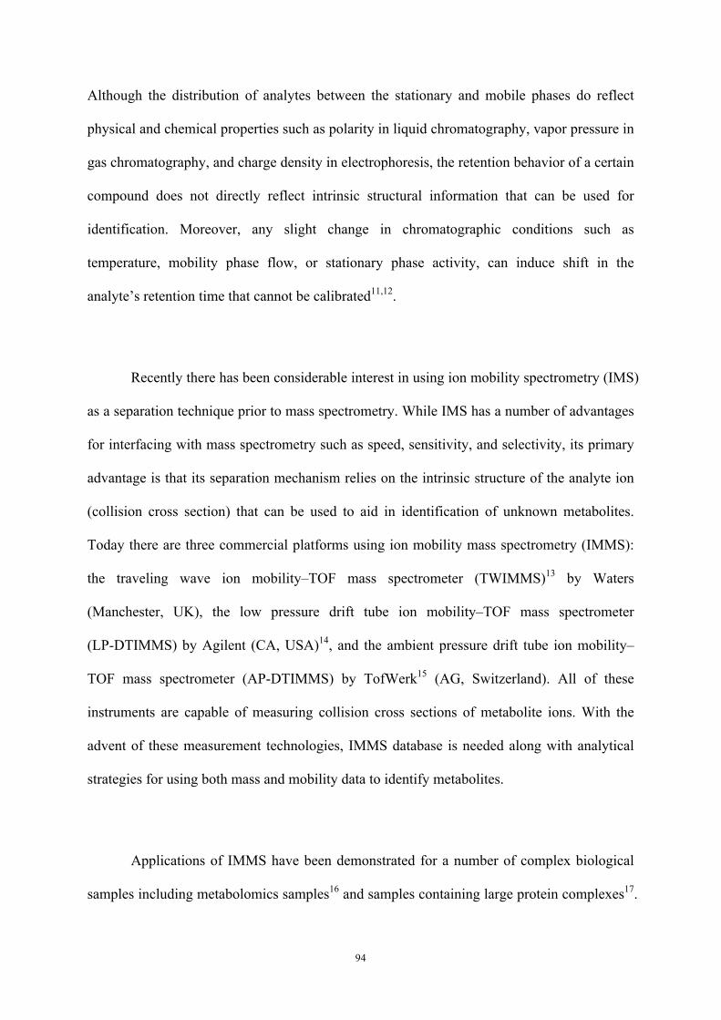
94

Although the distribution of analytes between the stationary and mobile phases do reflect

physical and chemical properties such as polarity in liquid chromatography, vapor pressure in

gas chromatography, and charge density in electrophoresis, the retention behavior of a certain

compound does not directly reflect intrinsic structural information that can be used for

identification. Moreover, any slight change in chromatographic conditions such as

temperature, mobility phase flow, or stationary phase activity, can induce shift in the

analyte’s retention time that cannot be calibrated11,12.

Recently there has been considerable interest in using ion mobility spectrometry (IMS)

as a separation technique prior to mass spectrometry. While IMS has a number of advantages

for interfacing with mass spectrometry such as speed, sensitivity, and selectivity, its primary

advantage is that its separation mechanism relies on the intrinsic structure of the analyte ion

(collision cross section) that can be used to aid in identification of unknown metabolites.

Today there are three commercial platforms using ion mobility mass spectrometry (IMMS):

the traveling wave ion mobility–TOF mass spectrometer (TWIMMS)13 by Waters

(Manchester, UK), the low pressure drift tube ion mobility–TOF mass spectrometer

(LP-DTIMMS) by Agilent (CA, USA)14, and the ambient pressure drift tube ion mobility–

TOF mass spectrometer (AP-DTIMMS) by TofWerk15 (AG, Switzerland). All of these

instruments are capable of measuring collision cross sections of metabolite ions. With the

advent of these measurement technologies, IMMS database is needed along with analytical

strategies for using both mass and mobility data to identify metabolites.

Applications of IMMS have been demonstrated for a number of complex biological

samples including metabolomics samples16 and samples containing large protein complexes17.

95

Human blood, in particular, offers an obvious target for the diagnoses of diseases through

metabolomics. Inborn errors in the genetic code have been diagnosed using metabolomics

since the 1980’s18. Other diseases such as type II diabetes19 and cardiovascular disease20 have

been diagnosed using metabolic profiling of blood samples. Recent interests are developing

on a wide range of other diseases including digestive21, metal,22 and pregnancy disorders23

have been investigated by metabolomics of blood samples.

Metabolite identifications are mainly based on the m/z information using metabolite

databases. Public databases have been developed over the past decade, among which, the

Human Metabolome Database (HMDB)24 and METLIN25 are two major databases containing

analytical and molecular information about human metabolites. HMDB aids metabolite

identification based on NMR and mass spectra. It provides information including metabolite

abundance, biological functions, and spectral viewing tools for a large number of metabolites.

METLIN is another online database focused on MS-based data, including comprehensive

MS/MS information, an annotated list of known metabolites and their chemical structures.

These databases remain under development due to the fact that whole human blood

metabolome is not complete. In addition, these databases lack structural information such as

reduced mobility values or collision cross section values, therefore, cannot distinguish

isomers.

The goal of this work is to produce mobility data for metabolites in human blood that

can be used in establishing IMMS database for metabolites, and to demonstrate analytical

strategies in which mobility and mass information can be combined to facilitate metabolite

identifications.

96


4.2.1 Sample Preparation:

SRM 1950 Metabolites in Human Plasma was provide by National Institute of

Standards and Technology (NIST). It consisted a plasma pool collected from an equal

number of men and women and with a racial distribution that reflects the U.S. population.

NIST SRM 1950 was sealed and stored at -80°C. A volume of 50 µL of SRM 1950 was

added into extraction solution (800 µL of HPLC grade methanol and 50 µL of HPLC grade

water). The mixture was kept at 60°C in water bath for 30 minutes, and then centrifuged at

13k RMP for 30 minutes. All supernatant was removed into a glass vial and evaporated by a

stream of clean nitrogen to a volume of 150 µL.

Human blood sample was collected from fingertip cleaned with a 70% alcohol pad

and air-dried. A sterile lancet was then used to prick the finger pad. Blood drops were

collected in a glass vial26. 900 µL HPLC grade methanol was used as extraction solution for

metabolite extraction. 50 µL blood was mixed with the extraction solution and kept at 60°C

in water bath for 30 minutes. The sample was then centrifuged at 13k RMP for 30 minutes.

Supernatant was further diluted with 1:4 v/v ratio of supernatant and electrospray solvent

(49.95:49.95:0.1 v/v/v of HPLC grade water, methanol and formic acid).

4.2.2 ESI-HT-IMtofMS Analysis:

Electrospray (ESI): Sample solution was introduced for IMMS analysis by a syringe

pump (model Fusion 200) (Chemyx Inc. TX). Fused silica capillary (Polymicro Inc. AZ) with

internal diameter of 150 µM was used as the electrospray source and sample introduction

loop. A biased voltage of 3000 volts and a sample solution flow rate of 3 µL/min were held

97

constant during the experiment.

Hadamard Transform ion mobility time-of-flight mass spectrometry (HT-IMtofMS)27:

A conventional stacked ring ion mobility spectrometer constructed in-house at Washington

State University, consisting of an 8cm long dissolvation region, a 22 cm long drift region and

a Bradbury-Nielsen (BN) ion gate. Hadamard transform signal was imposed on the BN ion

gate through a gate controller, allowing ion gate to open multiple times during an IMS cycle

to increase the throughput of the IMMS analysis. Both the dissolvation region and the drift

region were constructed using alternating stainless steel conducting rings and ceramic

insulating rings, where the conducting rings were connected with 1 MΩ resistors to create a

uniform electric field (305 V/cm in drift region). A nitrogen drift gas flow was introduced

into the IMS with a flow rate of 2.5 L/min. The IMS tube was held at a constant temperature

of 220°C and operated at ambient pressure (690-705 Torr). Ions were transmitted into a

time-of-flight mass spectrometer (tofMS) through an IMMS interface after IMS separation.

Both IMMS interface and tofMS were purchased from Tofwerk (Thun, Switzerland) and

operational details were descried elsewhere15. Note that the time-of-flight mass spectrometer

was operated in V-mode with a resolution of 5000-7000. The data acquisition software

(TofDaq) and processing software (IMSveiwer1_6d) were also provided by Tofwerk (Thun,

Switzerland).

ESI background spectra were collected using electrospray solvent before each sample

analysis and used for background extraction. Mobility calibration was conducted using

2,6-di-tert-butylpyridine (Sigma-Aldrich). Sodium ion and polydimethylsiloxane ion were

used for internal mass calibration. Each ESI-HT-IMMS analysis lasted for 2 - 3 minutes.

98

4.2.3 Multidimensional Data from ESI-HT-IMtofMS Analysis:

Data collected from ESI-HT-IMtofMS analysis produced a peak list containing

thousands of features characterized by drift time (td), mass-to-charge ratio (m/z) and intensity.

Drift time was recorded as the time required for an ion to travel through the IMS drift region.

It was then used to generate the mobility (K) of an ion species as shown in (1). Reduced

mobility constant shown in (2) remains constant for a given drift gas and E/N, since it

incorporates the pressure and temperature of the drift region.

Where V (volts) is the voltage drop across the IMS drift region with length L (cm), td is drift

time (s). P is the pressure (Torr) and T is the absolute temperature.

Besides reduced mobility values, collision cross-sections (Ω)14 were also obtained.

Collision cross section value reflects ionic size, which complements m/z information

provided by mass spectrometer. By combining m/z and Ω, we were able to assess ionic

density and compound classification. The derivitization of Ω is shown in (3), where e is the

charge on the ion, N is the drift gas number density, K is the mobility, k is Boltzmann’s

constant, T is the absolute temperature, and µ is the reduced mass (4) for the ion (m) and

neutral drift gas (M).

! = ! !!

!!! !!!!!!!!!!!!!!!!!!!!!!!!!!!!!!!!!!!!!!!!!!!!!!!(1)

!!!!!!!!!! =!!!!! !× !

273.15! !× ! !760 !!!!!!!!!!!!!!!!!!!!!!!!!!!!!!!(2)

Ω! = !3!

16!"2!!"# !!!!!!!!!!!!!!!!!!!!!(3)

99

Mobility mass correlation is based on a linear relationship between ionic mass (m/z) and

ionic size (Ω/z) 28,29. A specific class of compounds will provide a mobility mass correlation

with unique slope (a) and intercept (b), as shown in (5).

4.2.4 Data Processing for Metabolite Identifications:

Matching with NIST SRM 1950: Peak list generated from NIST SRM 1950 was used

to match with the peak list generated from human blood sample. The metabolite features

detected reproducibly in both samples were identified by matching with the NIST certificate

of analysis (COA) database30.

Matching with public metabolome databases: Human Metabolomes Database and

METLIN Metabolomics Database were applied in this study. The criteria for metabolite

identification included exact m/z obtained from the peak list, a mass accuracy of 10 – 30 ppm,

and adduct forms of [M+H]+, [M+Na]+, [M+K]+ and [M+H-H2O]+. By the above simple and

tentative identification procedure based on m/z, there could be multiple metabolite candidates

matched for one m/z. Therefore, further identification verification was necessary.

Identification based on mobility information: 1) isomeric separations were displayed

!! = ! !"! +! !!!!!!!!!!!!!!!!!!!!!!!!!!!!!!(4)

Ω! = ! !

! !+ !!!!!!!!!!!!!!!!!!!(5)

100

using selected-mass mobility analysis by showing multiple mobility peaks for the same m/z;

2) accurate isotopic ratio analysis was performed by measuring the peak areas of the ion

mobility peaks for targeted metabolite and its isotopes; 3) mobility mass correlation curves

were used to identify the classifications of unknown metabolite features; 4) protein ions with

different charge states formed a trend line which was used for calculating the molecular

weight of the protein, therefore, facilitated identification.

101


4.3.1 Metabolite Detection and Separation by ESI-HT-IMMS:

Figure 4.2 illustrates the mass and mobility information obtained from human blood

metabolome. 4.2a shows a typical 3-dimensional spectrum with x-axis representing m/z 100 -

1100, y-axis as drift time ranges from 15 ms to 85 ms, and z-axis as intensity; 4.2b and 4.2c

are the corresponding mass spectrum and ion mobility spectrum. Around ~1000 IMMS

features were detected and assigned with multidimensional information including m/z, drift

time and intensity. The 5000 - 7000 resolution of the TOF mass spectrometer allowed it to

distinguish metabolite features with m/z difference > 0.1. The resolving power of IMS was

80 - 120, sufficient to distinguish isomers and isobars that have small structural difference.

IMMS combined the separation power from both MS and IMS, allowing more metabolite

features to be detected when compared to MS analysis alone. Besides acting as size

separation apparatus, ion mobility spectrometer also prevented unwanted neutral molecules

and containments from entering the mass spectrometer. Neutral molecules especially solvent

molecules generated from electrospray ionization were kept away from the mass

spectrometer by the N2 buffer gas in IMS, therefore, MS can detect metabolite ions that are

completely desolvated. Moreover, IMS spread the noise from MS, efficiently reduced the

noise and increased the signal to noise ratio. Therefore, the overall analysis by

ESI-HT-IMMS was performed with improved signal to noise ratio when compared to using

MS alone.

4.3.2 Metabolite Identification using Databases:

Figure 4.1b and 4.1c display the major metabolite features detected in human blood

sample (250 metabolite features with m/z range from 100 to 1200) and NIST Plasma sample

102

(200 metabolite features with m/z range from 100 to 800), respectively. ~60 metabolite

features were reproducibly detected in both samples. These metabolite features were firstly

matched with the NIST COA database for identification. However, only 12 metabolite

features were identified. The reasons for the low yield of identification are: 1) The NIST

COA database30 contains only 110 metabolites, therefore, there are hundreds of metabolite

features remain unknown and/or not included in the NIST COA database; 2) The database

collected results from 52 different studies, therefore, it is not possible for one single study to

yield all the information. The results described above demonstrated that HT-IMMS analysis

was able to detected hundreds of metabolites in a few minutes, however, the identification

using NIST COA database alone was not sufficient.

Public metabolome databases HMDB and METLIN were then used for the

identifications of the metabolite features in human blood metabolome that were not identified

using the NIST COA database. Since the identification using HMDB and METLIN was

based on m/z only, there were often multiple candidate metabolites for each metabolite

feature. Therefore, reduced mobility information provided by HT-IMMS analysis was

coupled with m/z information to improve the identification procedure. Table 4.1 provides the

identification of 185 metabolite features using the above three databases, as well as using the

reduced mobility information. The measured m/z values, reduced mobility (K0) values, peak

heights, adduct forms, and identifications were reported.

4.3.3 Metabolite Identification using Mass and Mobility information -- Isotopic ratio

Analysis:

Natural isotopic pattern provides important information for compound identification.

103

Isotopic ratio analysis can be operated by mass spectrometer alone if targeted compounds

were known and without interferences. However, for the comprehensive detection of a whole

metabolome, it is difficult to obtain isotope measurement because the frequent occurrence of

multiple peaks within one mass unit. When ion mobility separation applied, isotopes that

belong to the same metabolite feature appear at same drift time because their size differences

are two small to be separated by IMS. Therefore, selected-mass mobility analysis can rapidly

distinguish the isotopes of a given metabolite feature by filtering out interference. Figure 4.3

shows an example of isotopic ratio analysis using IMMS. 4.3a is the mass spectra with x-axis

as mass range from 103.5 to 106.5 and y-axis as intensity. Three peaks with different m/z

values (104.11, 105.00 and 105.11) were shown in the mass spectra, however, it is difficult to

determine the existence of isotope pattern only by mass spectrometry because that each

individual mass peak could represent different metabolite features in the complex human

blood metabolome. 4.3b is the mass selected mobility spectra of m/z = 104.11 (blue), m/z =

105.00 (red) and m/z = 105.11 (green). The mobility peak of m/z 104.11 and m/z 105.11

showed up at the same drift time of 22.52 ms, demonstrating that m/z 105.11 was an isotope

of 104.11. Therefore, the peak area ratio of 104.11 and 105.11 (calculated to be 100: 5.5) was

used for the identification of metabolite feature with m/z 104.11. This metabolite feature was

identified as choline ion [C5H14NO]+. Isotope ratio analysis was observed and applied for

the identification of 8 metabolite features, including amino acid, peptides, fatty acids and

lipid. Table 4.2 shows the isotopic ratio analysis results including measured m/z, drift time,

K0, isotopic ratios, identified chemical formula proposed metabolite identification, and

adduct form.

104

4.3.4 Metabolite Identification using Mass and Mobility information – Isomers and Isobars

separation:

The existence of isomers and isobars in metabolomes has been a challenge for

metabolite detection and identification. Isomeric separation can be achieved easily and

rapidly with IMS. Isobars can be separated using high-resolution mass spectrometer alone,

however, with the application of IMS, they can be separated with low-resolution mass

spectrometer as well. The TOF mass spectrometer employed in this study was operated a

resolution of ~500 - 7000, which was not capable of separating isomers and isobars with m/z

differences less than 0.01. Figure 4.4 illustrates an example of IMS facilitating MS for

isobars separation. 4.4a is the zoomed-in mass spectrum with m/z ranges from 115.0 to 115.6.

It clearly detected one mass peak with broad peak width, which indicated the possibility of

isobars existence, however, the mass spectrometer was unable to distinguish between the

isobars. 4.4b shows the selected mass ion mobility spectrum of the targeted mass peak. With

two mobility peaks detected by IMS, confirming the existence of isobars. The identification

of the mobility peak at 22.6 ms was [N-mononitrosopiperazine+H]+ with m/z of 115.08 K0 of

2.08, and the later mobility peak at 23.6 ms was identified as [Gamma-caprolactone+H]+ with

m/z of 115.07 and K0 of 1.99.

5 pairs of isomers/isobars were detected by IMMS, and Table 4.3 summarized the

information for each metabolite feature including measured m/z, reduced drift time, K0,

metabolite identification, adduct form. The enhanced separation power using IMS also

demonstrated that the addition of IMS can increase peak capacity.

105

4.3.5 Metabolite Identification using Mass and Mobility information – Charge States

Separation:

Ion charge states separation has been reported as another unique merit from IMMS

analysis. Mass spectrometry can differentiate charge states based on the m/z values, while

IMMS can separate and present them into the two dimensional IMMS space. Figure 4.5 is

the IMMS two-dimensional spectra of a protein detected with charge states from +13 to +17.

As shown in the spectra, a trend line was formed with good linearity and increasing m/z

difference (Δm/z) between two adjunct charge states. The different Δm/z values were used

for the identification of hemoglobin and its charge states.

The detailed information of these protein features is listed in Table 4.1, from m/z

895.51 to 1173.91. It is clear that the overall reduced mobility values for hemoglobin ion

species were smaller when compared with the other metabolite features, demonstrating its

compact ionic structure. Moreover, multiple mass peaks were detected within each charge

state, showing the complex isotopic pattern of protein.

4.3.6 Metabolite Identification using Mass and Mobility information – Mobility-mass

Correlations:

The collision cross section to charge ratio (Ω/z) is a property measured by IMS and

directly related to the ionic size and structure. Ω/z can be helpful in identifying an ion

analogously to m/z. Moreover, in the IMMS 2-dimensional space, Specific compound class

tends to form unique mobility-mass correlation, providing class identifications not possible

by any other methods14,31.

106

In the IMMS spectrum, these mobility-mass correlations appear as trend lines with

specific slopes and intercepts that can also be used to provide qualitative information for the

identification of unknowns. Figure 4.6 shows the IMMS 2-dimensional spectra, illustrating

the classification trend lines detected in human blood metabolome. The x-axis represents m/z

ranged from 100 to 1100 and y-axis represents drift time ranged from 15 ms to 90 ms. Five

classification trend lines for amino acids, peptides, and phospholipids were identified and

plotted. Metabolite features fell along a certain trend line were either belonged to that class or

shared structural similarities to that classification of compounds.

In order to better explain the mobility-mass correlations, linear relationships between

1/K0 and m/z were obtained and shown in Table 4.4. With R2 values ranged from 0.89 to

0.99, the correlations were confirmed with good linearity. Since Ω/z is directly proportional

to 1/K0, the results well explained that the relationship between ion’s size-to-charge ratio and

mass-to charge ratio is classification specific. The most recent work by May et al.14

investigated four chemically distinct classes of compounds including quaternary ammonium

salts, lipids, peptides, and carbohydrates, showing near-linear polynomial fits between m/z

and Ω/z. The difference between the result by May and the result here is mainly due to the

different m/z ranges. May et al. studied the correlation in m/z ranging from 200 to near 2000.

However, in this study, a smaller m/z range was investigated.

107

4.4 Conclusions

HT-IMMS analysis enables high throughput and comprehensive metabolite detection

in both NIST SRM 1950 sample and human blood sample, with both ion mobility separation

and m/z detection within 2-3 minutes. It is clear that NIST SRM 1950 and its COA database

are insufficient for metabolite identification for human blood metabolome. With the help of

HMDB and METLIN, metabolite identification is improved, however, still has problems

such as multiple candidates for each metabolite feature. IMMS technique provides reduced

mobility information associated with ionic structure, facilitating metabolite identification. It

allows accurate isotopic ratio analysis without interference; isomers/isobars separation to

increases the peak capacity. It also provides mobility-mass correlations that add qualitative

information regarding to compound classifications. With over a thousand metabolite features

detected and 185 metabolite features identified, it is evident that IMMS is an efficient method

for comprehensive metabolite detection, and the strategies for metabolite identification using

both mobility and mass information yields more reliable identifications. However, generating

IMMS database for metabolome is necessary to further aid metabolite identification.

108

Reference (1) Nordström, A.; Lewensohn, R. J Neuroimmune Pharmacol 2009, 5, 4–17.

(2) Nicholson, J. K.; Lindon, J. C. Nature 2008, 455, 1054–1056.


(4) Brown, S. C.; Kruppa, G.; Dasseux, J. L. Mass Spectrom. Rev. 2005, 24, 223–231.

(5) Hu, Q.; Noll, R. J.; Li, H.; Makarov, A.; Hardman, M.; Graham Cooks, R. J. Mass

Spectrom. 2005, 40, 430–443.

(6) Wilson, I. D.; Nicholson, J. K.; Castro-Perez, J.; Granger, J. H.; Johnson, K. A.;

Smith, B. W.; Plumb, R. S. J. Proteome Res. 2005, 4, 591–598.

(7) Schauer, N.; Steinhauser, D.; Strelkov, S.; Schomburg, D.; Allison, G.; Moritz, T.;

Lundgren, K.; Roessner-Tunali, U.; Forbes, M. G.; Willmitzer, L.; Fernie, A. R.;

Kopka, J. FEBS Letters 2005, 579, 1332–1337.

(8) Theodoridis, G. A.; Gika, H. G.; Want, E. J.; Wilson, I. D. Analytica Chimica Acta

2012, 711, 7–16.

(9) Dunn, W. B.; Erban, A.; Weber, R.; Creek, D. J.; Brown, M. Metabolomics 2013.

(10) Prasad, B.; Garg, A.; Takwani, H.; Singh, S. Trends in Analytical Chemistry 2011,

30, 360–387.

(11) Creek, D. J.; Jankevics, A.; Breitling, R.; Watson, D. G.; Barrett, M. P.; Burgess, K.

E. V. Anal. Chem. 2011, 83, 8703–8710.

(12) Castillo, S.; Gopalacharyulu, P.; Yetukuri, L.; Orešič, M. Chemometrics and

Intelligent Laboratory Systems 2011, 108, 23–32.


1559–1566.

(14) May, J. C.; Goodwin, C. R.; Lareau, N. M.; Leaptrot, K. L.; Morris, C. B.;

Kurulugama, R. T.; Mordehai, A.; Klein, C.; Barry, W.; Darland, E.; Overney, G.;

109

Imatani, K.; Stafford, G. C.; Fjeldsted, J. C.; McLean, J. A. Anal. Chem. 2014, 86,

2107–2116.




Anal. Chem. 2009, 81, 7944–7953.

(17) Ruotolo, B. T.; Benesch, J. L. P.; Sandercock, A. M.; Hyung, S.-J.; Robinson, C. V.

Nat Protoc 2008, 3, 1139–1152.

(18) Ramautar, R.; Berger, R.; van der Greef, J.; Hankemeier, T. Current Opinion in

Chemical Biology 2013, 17, 841–846.

(19) Wang-Sattler, R.; Yu, Z.; Herder, C.; Messias, A. C.; Peters, A.; Meitinger, T.;

Roden, M.; Wichmann, H.-E.; Pischon, T.; Adamski, J.; Illig, T. Mol. Syst. Biol.

2012, 8, 615.

(20) Shah, S. H.; Bain, J. R.; Muehlbauer, M. J.; Stevens, R. D.; Crosslin, D. R.; Haynes,

C.; Dungan, J.; Newby, L. K.; Hauser, E. R.; Ginsburg, G. S.; Newgard, C. B.;

Kraus, W. E. Circ Cardiovasc Genet 2010, 3, 109.

(21) Schicho, R.; Shaykhutdinov, R.; Ngo, J.; Nazyrova, A.; Schneider, C.; Panaccione,

R.; Kaplan, G. G.; Vogel, H. J.; Storr, M. J. Proteome Res. 2012, 11, 3344–3357.

(22) Bogdanov, M.; Matson, W. R.; Wang, L.; Matson, T.; Saunders-Pullman, R.;

Bressman, S. S.; Beal, M. F.; Flint Beal, M. Brain 2008, 131, 389–396.

(23) Diaz, S. O.; Pinto, J.; Graça, G.; Duarte, I. F.; Barros, A. S.; Galhano, E.; Pita, C.; do

Céu Almeida, M.; Goodfellow, B. J.; Carreira, I. M.; Gil, A. M. J. Proteome Res.

2011, 10, 3732–3742.



110




Shaykhutdinov, R.; Li, L.; Vogel, H. J.; Forsythe, I. Nucleic Acids Research 2009,

37, D603–D610.

(25) Smith, C. A.; O'Maille, G.; Want, E. J.; Qin, C. Therapeutic drug … 2005.

(26) Bruce, S. J.; Jonsson, P.; Antti, H.; Cloarec, O.; Trygg, J.; Marklund, S. L.; Moritz,

T. Analytical Biochemistry 2008, 372, 237–249.

(27) Zhang, X.; Knochenmuss, R.; Siems, W. F.; Liu, W.; Graf, S.; Hill, H. H. Anal.

Chem. 2014, 86, 1661–1670.

(28) Fenn, L. S.; Kliman, M.; Mahsut, A.; Zhao, S. R.; McLean, J. A. Anal Bioanal Chem

2009, 394, 235–244.

(29) McLean, J. A.; Ruotolo, B. T.; Gillig, K. J.; Russell, D. H. International Journal of

Mass Spectrometry 2005.

(30) Simón-Manso, Y.; Lowenthal, M. S.; Kilpatrick, L. E.; Sampson, M. L.; Telu, K. H.;

Rudnick, P. A.; Mallard, W. G.; Bearden, D. W.; Schock, T. B.; Tchekhovskoi, D.

V.; Blonder, N.; Yan, X.; Liang, Y.; Zheng, Y.; Wallace, W. E.; Neta, P.; Phinney,

K. W.; Remaley, A. T.; Stein, S. E. Anal. Chem. 2013, 85, 11725–11731.

(31) Woods, A. S.; Ugarov, M.; Egan, T.; Koomen, J.; Gillig, K. J.; Fuhrer, K.; Gonin,

M.; Schultz, J. A. Anal. Chem. 2004, 76, 2187–2195.

111

Table 4.1 Metabolite identification of 185 major metabolite features detected by

HT-IMtofMS. Measured m/z, drift time and K0 are included.

m/z Drift time Ko

Peak Height Metabolite Identification Adduct

100.083 22.20 2.11 447.067 5-aminopentanoic acid [M+H-H2O]+ 102.099 23.21 2.02 735.271 Betaine aldehyde [M+H]+ 104.115 22.51 2.08 7993.72 Choline [M+H]+ 105.000 24.82 1.89 1365.29 Mercaptolactic acid [M+H-H2O]+ 108.052 24.55 1.91 484.306 3-Pyridinaldehyde [M+H]+ 114.075 23.14 2.03 836.098 Creatinine [M+H]+ 115.083 22.55 2.08 115.857 N-Mononitrosopiperazine [M+H]+ 115.083 23.60 1.99 106.525 gamma-caprolactone [M+H]+ 116.081 23.55 1.99 86.3621 Proline [M+H]+ 119.029 23.46 2.00 208.848 Succinic acid [M+H]+ 121.045 23.39 2.01 112.681 Purine [M+H]+ 121.079 23.40 2.01 260.592 4-Dexyerythronic [M+H]+ 122.067 25.98 1.81 270.43 Benzamide [M+H]+ 123.059 23.82 1.97 413.057 Niacinamide/Vitamine B3 [M+H]+ 124.079 26.73 1.76 162.874 5-aminopentanal [M+H]+ 129.067 23.86 1.97 116.565 Dihydrothymine [M+H]+ 132.097 24.27 1.93 214.551 Leucine/Isoleucine [M+H]+ 133.047 24.45 1.92 236.101 Methylsuccinic acid/glutaric acid [M+H]+ 135.060 25.19 1.86 119.312 Homocysteine thiolactone [M+NH4]+ 136.058 25.50 1.84 775.11 Homocysteine [M+H]+ 137.073 25.52 1.84 270.92 N-Mononitrosopiperazine (not sure) [M+Na]+ 138.062 25.85 1.82 175.774 PABA (p-Aminobenzoic acid) [M+H]+ 139.063 26.02 1.80 104.819 8-Hydroxypurine [M+H]+ 139.075 24.81 1.89 101.507 Isocapronic acid [M+Na]+ 140.076 26.04 1.80 471.938 Valine [M+Na]+ 145.042 25.50 1.84 149.583 3-Methylglutaconic acid [M+H]+ 146.070 25.51 1.84 174.778 N/A N/A 147.123 26.06 1.80 124.781 Lysine [M+H]+ 148.060 25.40 1.85 89.8962 Glutamic acid [M+H]+ 152.033 25.41 1.85 401.62 Pyruglutamic acid [M+Na]+ 154.071 26.61 1.76 229.604 Fapy-adenine [M+H]+ 156.051 26.06 1.80 964.567 Histidine [M+H]+ 157.091 26.29 1.79 377.044 Cymene [M+Na]+ 158.066 26.63 1.76 794.719 2-Phenylacetamide [M+Na]+ 159.017 28.50 1.65 82.1021 Erythronic acid [M+Na]+ 163.049 27.29 1.72 216.752 N/A N/A 166.092 27.89 1.68 653.803 Phenylalanine [M+H]+ 169.069 26.52 1.77 84.1626 Uric acid [M+H]+ 170.041 26.61 1.76 243.095 Glutamate [M+Na]+

112

175.144 27.77 1.69 95.3766 Arginine [M+H]+ 182.069 27.92 1.68 815.838 Tyrosine [M+H]+ 184.085 29.75 1.58 133.138 Vitamin B6 [M+H]+ 187.004 28.28 1.66 1590.47 3-phosphoglyceric acid (3PG) [M+H]+ 200.075 29.87 1.57 219.577 N/A N/A 203.060 29.70 1.58 860.53 Glucose [M+Na]+ 203.060 28.47 1.65 263.581 Fructose [M+Na]+ 214.182 31.75 1.48 163.819 N/A N/A 219.034 29.62 1.58 182.375 Tyrosol 4-sulfate [M+H]+ 228.201 33.07 1.42 1031.76 N/A N/A 235.017 29.52 1.59 586.36 N/A N/A 236.164 33.58 1.40 900.538 N,O-Didesmethyltramadol [M+H]+ 238.176 34.05 1.38 227.167 12-amino-dodecanoic acid [M+Na]+ 245.131 32.82 1.43 147.86 Phe-Pho [M+H]+ 250.181 34.94 1.34 2930.05 Lophocerine [M+H]+ 252.151 34.19 1.37 96.4383 N-Decanoylglycine [M+Na]+ 254.153 34.74 1.35 159.059 Gamma-Aminobutyryl-lysine [M+Na]+ 256.268 40.85 1.15 732.798 Palmitic amide [M+H]+ 266.156 35.65 1.32 1166.71 Proline-lysine [M+H]+ 267.127 34.80 1.35 129.335 Phe-Thr [M+H]+ 268.069 33.19 1.41 112.562 Asp-Pro [M+K]+ 268.121 35.63 1.32 587.795 Adenosine [M+H]+ 269.003 33.94 1.38 1057.21 Dimethylallyl pyrophosphate [M+Na]+ 278.241 40.70 1.15 961.488 Palmiti amide [M+Na]+ 279.163 37.17 1.26 230.189 leu-phe [M+H]+ 282.206 36.82 1.27 547.689 Colestipol [M+H]+ 284.296 43.34 1.08 327.502 Sphinganine [M+H-H2O]+ 289.156 39.96 1.17 1640.88 Asparaginyl-arginine [M+H]+ 298.175 37.59 1.25 474.856 Ser-Leu-Pro [M+H-H2O]+ 301.142 39.76 1.18 4428.7 Gly-Gly-Pro-Ala [M+H]+ 302.246 39.70 1.18 747.329 linoleamides [M+Na]+ 303.229 39.57 1.19 899.109 Linoleic acid [M+Na]+ 304.257 41.31 1.14 366.859 Oleamide/Elaidamide [M+Na]+ 305.132 39.80 1.18 818.769 YC-1 [M+H]+ 306.278 42.98 1.09 256.441 Linoleoyl ethanolamide [M+H-H2O]+ 317.114 39.92 1.18 2123.1 glutamy-phenylalanine [M+Na]+ 318.212 40.70 1.15 123.949 N/A N/A 319.121 39.99 1.17 107.902 N/A N/A 325.205 42.30 1.11 129.806 Dinor-PGD2 [M+H]+ 326.234 41.19 1.14 404.939 10-Nitrolinoleic acid [M+H]+ 327.229 41.02 1.14 178.514 Eicosatetraenoic acid (C20:4n) [M+H]+ 332.291 43.56 1.08 522.628 Oleol Ethyl Amide [M+H]+ 335.144 39.70 1.18 240.563 Met-Ala-Asn [M+H]+ 338.337 47.10 1.00 1424.69 N-cyclohexanecarbonylpentadecylamine [M+H]+ 339.338 46.58 1.01 119.882 4,6-Docosanedione [M+H]+

113

342.221 42.06 1.12 159.748 Arachidonoyl amine [M+K]+ 342.328 47.50 0.99 122.611 N,N,N-trimethyl-spingosine [M+H]+ 354.403 50.79 0.92 2089.75 Tetracosene [M+NH4]+ 359.248 42.67 1.10 336.586 2-Hydroxydesogestrel [M+Na]+ 360.318 45.84 1.02 7979.99 13-Docosenamide [M+Na]+ 369.344 46.26 1.01 2251.7 Cholesterol [M+H-H2O]+ 376.294 47.07 1.00 2363.97 13-Docosenamide [M+K]+ 383.322 46.35 1.01 547.388 4,6-cholestadienone [M+H]+ 385.342 48.28 0.97 248.419 PreVitamine D3 [M+H]+ 385.342 47.43 0.99 98.2378 Dehydrocholesterol [M+H]+ 387.190 44.55 1.05 135.668 Pro-Glu-Ala-Ala [M+H]+ 388.344 48.12 0.98 220.69 Aminopentol [M+H-H2O]+ 392.289 48.20 0.97 220.051 12-HETE-Ala [M+H]+ 392.289 47.73 0.98 167.352 15-HEYE-Ala [M+H]+ 398.237 47.20 0.99 176.486 Lys-Pro-Gly-Pro [M+H]+ 405.309 50.81 0.92 374.007 Cholesta-4,6-dien-3-one [M+Na]+ 409.164 45.92 1.02 955.715 Pro-Glu-Ala-Ala [M+Na]+ 413.258 49.67 0.94 710.818 Lyso PC(10:0) [M+H]+ 414.221 47.74 0.98 222.726 Arg-Trp-Ala [M+H-H2O]+ 425.142 45.87 1.02 812.838 His-Phe-OH [M+H]+ 426.327 52.13 0.90 175.69 Oleoylcarnitine [M+H]+ 429.231 49.76 0.94 280.347 Pro-Glu-Ala-Leu [M+H]+ 429.353 52.03 0.90 145.373 N/A N/A 452.273 49.19 0.95 102.959 Arg-Val-Arg [M+Na]+ 469.340 54.05 0.87 547.633 PC(P-14:0/0:0) [M+NH4]+ 496.319 55.98 0.84 276.148 His-Ile-Lys-Val [M+H]+ 518.289 57.35 0.82 661.48 PC(15:0) [M+Na]+ 524.330 58.45 0.80 103.811 Val-Arg-Leu-His [M+H]+ 534.268 57.68 0.81 1115.28 Arg-Cys-Gln-Lys [M+H]+ 542.310 56.36 0.83 107.895 Asn-Pro-Arg-Arg [M+H]+ 544.299 57.95 0.81 232.752 His-Arg-Leu-Pro [M+H]+ 546.320 59.58 0.79 215.682 PE(20:0) [M+Na]+ 547.315 59.67 0.79 176.969 Cys-Arg-Ile-Arg [M+H]+ 558.258 57.21 0.82 169.582 Tyr Thr Phe Gln [M+Na]+ 560.266 58.57 0.80 168.845 Tyr Lys Tyr Ser [M+H]+ 562.284 59.95 0.78 271.205 Arg Gln Gln Met [M+H]+ 617.468 65.48 0.72 103.518 PA(31:1) [M+H]+ 637.263 63.21 0.74 1313.86 Ser-His-Trp-Trp [M+Na]+ 659.241 66.93 0.70 3006.61 Try-Try-Try-Glu [M+Na]+ 671.526 70.46 0.67 3748.32 PA(36:1) [M+H-H2O]+ 673.548 71.00 0.66 730.614 PE-Cer(d14:2(4E,6E)/21:0) [M+H]+ 675.214 66.95 0.70 2732.84 Try-Try-Try-Glu [M+K]+ 687.500 71.28 0.66 272.554 PA(35:2) [M+H]+ 688.506 71.29 0.66 244.606 PC(29:2) [M+H]+ 695.518 71.36 0.66 613.483 PA(35:1) [M+Na]+

114

696.502 71.41 0.66 133.634 PE(34:4) [M+H]+ 697.503 71.47 0.66 107.713 PA(35:0) [M+Na]+ 697.503 72.03 0.65 102.148 PA(P-35:0) [M+Na]+ 711.474 72.56 0.65 83.1371 PA(35:1) [M+Na]+ 725.495 74.18 0.63 309.569 PA(38:4) [M+H]+ 726.495 74.31 0.63 291.408 PE(35:4) [M+H]+ 741.416 74.85 0.63 82.4017 PG(31:3) [M+K]+ 741.475 74.75 0.63 88.7288 PG(32:2) [M+Na]+ 758.510 74.41 0.63 466.089 PC(31:0) [M+K]+ 780.487 74.86 0.63 932.707 PS(36:6) [M+H]+ 782.497 75.04 0.63 497.505 PS (34:2) [M+Na]+ 782.497 76.17 0.62 366.676 PS (36:5) [M+H]+ 796.459 75.70 0.62 1297.31 PS(34:3) [M+K]+ 797.438 76.18 0.62 169.417 PI(30:4) [M+Na]+ 798.454 76.81 0.61 156.723 PS(34:2) [M+K]+ 805.435 75.56 0.62 91.568 PG(36:6) [M+K]+ 806.508 75.76 0.62 219.982 PS (38:7) [M+H]+ 810.502 76.99 0.61 89.1405 PE(42:11) [M+H]+ 820.460 75.74 0.62 126.834 PS(36:5) [M+K]+ 822.471 76.54 0.61 115.621 PS(36:4) [M+K]+ 823.490 76.33 0.61 84.0074 PG(37:4) [M+K]+ 824.480 77.70 0.60 228.71 PS(36:3) [M+K]+ 825.500 77.64 0.60 150.98 PG(37:3) [M+K]+ 830.479 76.32 0.61 124.587 PS(40:9) [M+H]+ 832.529 77.35 0.61 108.391 PC(37:5) [M+K]+ 844.434 76.85 0.61 102.216 PS(38:7) [M+K]+ 895.507 62.86 0.75 98.7142 Hemoglobin [M+17H]17+ 947.831 64.59 0.73 121.932 Hemoglobin [M+16H]16+

1009.090 66.76 0.70 135.644

Hemoglobin [M+15H]15+

1009.140 66.74 0.70 85.9929 1009.220 66.76 0.70 156.075 1009.330 66.71 0.70 164.246 1009.400 66.68 0.70 145.386 1010.550 66.53 0.71 171.284 1010.610 66.67 0.70 100.171 1012.170 66.62 0.70 108.139 1012.400 66.52 0.71 86.9916 1014.670 66.61 0.70 108.922 1081.230 68.87 0.68 392.524


1081.380 69.08 0.68 83.1947 1084.120 68.60 0.68 178.559 1085.990 68.55 0.68 136.906 1087.090 68.53 0.68 133.202 1088.630 68.70 0.68 93.0488 1090.040 68.69 0.68 118.392

115

1091.350 68.71 0.68 95.4981 1095.170 68.83 0.68 82.4147 1164.180 71.54 0.66 80.4191


1164.440 71.61 0.66 274.278 1167.280 71.47 0.66 122.149 1167.710 71.31 0.66 102.511 1169.160 71.43 0.66 139.595 1169.300 71.34 0.66 87.5275 1169.300 71.48 0.66 85.6067 1170.970 71.39 0.66 101.411 1173.910 71.41 0.66 101.638

116

Table 4.2 Isotopic ratio analysis results.

# m/z Drift Time Ko Isotopic

Ratio Chemical Formula Metabolite Adduct

Form

1 104.115 22.51 2.08 100%

C5H14NO Choline [M]+ 105.117 22.53 2.08 6%

2 301.142 39.76 1.18 100%

C18H20O4 5-O-Methyllatifolin [M+H]+ 302.145 39.74 1.18 21%

3 317.114 39.92 1.18 100%

C11H18N4O8 Asp Gly Ser Gly [M+H-H2O]+ 318.119 39.96 1.18 13%

4 360.318 45.84 1.02 100%

C22H43NO 13-Docosenamide [M+Na]+ 361.320 45.87 1.02 24% 362.319 45.88 1.02 4%

5 376.294 47.07 1.00 100%

C22H43NO 13-Docosenamide [M+K]+ 377.291 47.10 1.00 24%

6 534.268 57.68 0.81 100%

C20H39N9O6S Arg Cys Gln Lys [M+H]+ 535.283 57.65 0.81 26%

7 659.241 66.93 0.70 100%

C32H36N4O10 Try Try Try Glu [M+Na]+ 660.244 66.95 0.70 32%

8 675.214 66.95 0.70 100%

C32H36N4O10 Try Try Try Glu [M+K]+ 676.218 66.93 0.70 32%

Table 4.3 Isomer/isobar separation and analysis results.

Metabolite Features m/z Drift

Time Ko Chemical Formula Metabolite Adduct

Form 1 115.087 22.55 2.08 C5H10N2O N-Mononitrosopiperazine [M+H]+ 2 115.076 23.60 1.99 C6H10O2 gamma-caprolactone [M+H]+

3 203.053 29.70 1.58 C6H12O6 Glucose [M+Na]+ 4 203.053 28.47 1.65 C6H12O6 Fructose [M+Na]+

5 383.331 46.35 1.01 C27H42O 24-Dehydroprovitamin D3 [M+H]+ 6 383.331 47.20 0.99 C27H42O 4,6-cholestadienone [M+H]+

7 385.347 48.28 0.97 C27H44O 4,6-cholestadienol [M+H]+ 8 385.347 47.43 0.99 C27H44O Vitamin D3 [M+H]+

9 782.494 75.04 0.63 C40H74NO10P PS 34:2 [M+Na]+

10 782.497 76.17 0.62 C42H72NO10P PS 36:5 [M+H]+

117

Table 4.4 Mobility-mass correlation trend lines.

Compound Classification Mobility-mass Correlation

Trend Line R2 Glycerophospholipid (PI) y = 0.0005x + 1.3805 0.89

Glycerophospholipid (PC, PS, PE) y = 0.0008x + 0.9727 0.90 Lyso-phospholipid y = 0.0014x + 0.5089 0.97

Tetrapeptide y = 0.0011x + 0.6337 0.86 Amino acid and Dipeptide y = 0.0018x + 0.2908 0.99

118

Figure 4.1 (a) Schematic diagram of the instrument: Electrospray ionization hadamard

transform atmospheric pressure ion mobility time-of-flight mass spectrometer; (b) major

metabolite features detected in human blood metabolome; (c) major metabolite features

detected in NIST SRM 1950.

a

b c

119

Figure 4.2 Global metabolomics results from HT-IMtofMS analysis. (a) shows the

multidimensional information of the metabolite features detected from human blood, with

x-axis as m/z (ranges from 100 to 1100), y-axis as drift time (ranges from 15 ms to 85 ms)

and z-axis as intensity. (b) and (c) are the corresponding mass spectrum and mobility

spectrum. Over a thousand metabolite features were detected during the analysis.

120

Figure 4.3 An example of accurate isotopic ratio analysis. (a) is the mass spectrum with

zoomed-in mass range from 103.5 to 106.5. Three m/z features were detected with m/z =

104.11, 105.00 and 105.11. (b) is the ion mobility spectra for the above three m/z features.

The mobility peak of m/z 105.11 overlapped with the mobility peak of m/z 104.11, indicating

its identity as an isotope of m/z 104.11.

121

Figure 4.4 An example of isomer/isobar separation. The mass spectrum with zoomed-in mass

range from 115.0 to 115.6 is shown in (a), with one m/z feature detected. (b) is the

corresponding ion mobility spectrum with two ion mobility peaks detected with drift time of

22.6 ms and 23.6 ms, demonstrating the existence of two different metabolite features

identified as [N-mononitrosopiperazine+H]+ and [Gamma-caprolactone+H]+.

122

Figure 4.5 IMMS two-dimensional spectrum of hemoglobin with charge states from +13 to

+17. Good linearity was observed with increasing m/z difference between two adjunct charge

states. This trend lines is also shown in Figure 4.6.

123

Figure 4.6 IMMS two-dimensional spectrum illustrating the metabolomes of human blood.

Each dot observed in this 2D space represents a metabolite feature. Six trend lines were

identified for different compound classification.

124

Chapter 5

Neuronal Metabolomics by Ion Mobility Mass Spectrometry in

Cocaine Self-administering Rats after Early and Late Withdrawal

Abstract

The neuronal metabolomes in rat striatum (STR), prefrontal cortex (PFC) and nucleus

accumbens (NAC) were analyzed by hadamard transform ion mobility mass spectrometry

(HT-IMMS) in order to reveal global and specific metabolic changes induced by cocaine

self-administration after 1-day or 3-weeks withdrawal. Metabolites were comprehensively

separated and detected with the employment of HPLC-IMMS within minutes. Global

metabolic differences were observed using PCA for comparisons between cocaine and saline

treatments after 1-day withdrawal. Potential biomarkers were selected using PCA loadings

plot and unpaired t-test, yielding a complete profile of metabolic changes induced by cocaine

self-administration. Metabolites associated with oxidative stress and energy metabolism were

also specifically investigated. We found out that the dysregulation of creatine/creatinine was

different between the STR and NAC, demonstrated that metabolic alterations are brain

regionally specific. Glutathione and adenosine were also changed in their concentrations, and

the results agreed with previous studies. In general, our findings support the multi-event

mechanism of cocaine-induced disorders proposed by previous investigations, and reveal

additional metabolic targets of cocaine-induced changes after early and extended withdrawal

times.

125

5.1 Introduction

As the second most commonly used illicit drug in the United States, cocaine affects

the lives and health of millions of people. The adverse health consequences to the individual

and the cost to society of cocaine abuse are substantial. Long term users are at greatly

increased risk for neurologic and cardiovascular toxicities as well as other complications1.

The mental elements in play with cocaine withdrawal include craving, exhaustion,

restlessness and depression, making cocaine one of the most addictive drugs2,3.

Classic mechanisms involved in cocaine addiction are increases in dopaminergic

transmission within striatal regions and altered glutamate transmission4,5. Previous

investigations have mainly centered on receptor binding and blocking of enzymes6. However,

additional studies7,8 suggest that the brain states caused by cocaine addiction are produced by

multi-events problems including oxidative stress, aberrant metabolism and

neuroinflammation, leaving a fuller explanation of the mechanisms unsolved. Moreover,

although cocaine withdrawal often has no visible physical symptoms, a severe level of

craving coupled with the lack of effective medications for reducing the craving, causes high

rates of relapse9,10. To better understand the addiction and withdrawal mechanism, it is

necessary to have a comprehensive interpretation of the concert of biochemical events

occurring after cocaine exposure and withdrawal from cocaine exposure.

Global metabolomics, as an exploratory investigation approach, simultaneously and

126

comprehensively measures metabolites to reveal changes in the metabolome. It not only

complements genomics and proteomics data, but also identifies phenotypic changes caused

by stimuli more predicatively than other “omics” approaches11. By measuring all metabolites

in a biological system, global metabolomics provides information for global metabolic

profiling and for the interrogation of specific metabolites of interest. Recent advances in

analytical techniques and data processing software has assisted the relatively new field of

metabolomics. The practice of metabolomics has grown rapidly, being applied to a wide

range of central nervous system diseases including schizophrenia and Parkinson’s disease12,13.

Effects on the metabolome from drug abuse such as cocaine, methamphetamine and

morphine have also been studied14,15.

Previous studies on drug abuse using metabolomics approaches have demonstrated

the potential of global metabolomics and the concept of the multi-event mechanism for

cocaine addiction. Patkar et al.15 performed metabolomics analysis on plasma samples from

cocaine-dependent individuals and drug-free controls using a liquid chromatography

electrochemical array platform, and discovered significant up-regulation in

n-methylserotonine and guanine, while hypoxanthine and xanthine were down regulated.

Metabolomics in brain tissues from cocaine treated rats was investigated by Li et al. using

1H-NMR16. Changes in the tissue concentrations of creatine, taurine, and N-acetylasparate

after cocaine treatment were observed, providing metabolic alterations associated with

neuotransmitters, oxidative stress and mitochondria dysregulation.

127

Comprehensive detection of metabolites with different concentrations, volatilities

and polarities is critical for understanding changes in the metabolome of different brain

regions caused by cocaine addiction. However, previous investigations have the common

problem of lacking comprehensive metabolomics analysis due to limited sensitivity.

IMMS17-19 has been well characterized as an efficient method for metabolomics by a number

of studies in tissues, biofluids, and cell lines. In this study, we employed hadamard transform

ion mobility mass spectrometry (HT-IMMS)20 for metabolomics analysis with its capability

of rapid analysis with nano-molar limit of detection, isomeric separation and generation of

two-dimensional information. We performed global metabolomics on multiple brain tissues

(striatum (STR), prefrontal cortex (PFC) and nucleus accumbens (NAC)) from rats under

cocaine administration followed by different withdrawal times (1 day and 3 weeks).

We predicted that cocaine self-administration would increase or decrease the levels of

multiple metabolites, and that these effects would be both brain region dependent and

withdrawal time dependent. The aim of this study was to investigate the addiction and

withdrawal effects of cocaine on the metabolomes of multiple brain regions globally and

specifically. Our goal was to select regionally specific potential biomarkers, and specifically

exam those biomarkers involved in energy metabolism and oxidative stress for demonstrating

the proposed multi-event mechanism of cocaine addiction.

128

5.2 Experimental Design

5.2.1 Subjects, Cocaine Self-administration and Brain Dissection:

Male Sprague-Dawley rats (300-330 gram) were singly housed in a temperature and

humidity-controlled room with a 12 hr light/dark cycle, with food and water provided ad

libitum except for when animals were engaged in experiments. Experiments were conducted

according to the National Institutes of Health Guide for the Care and Use of Laboratory

Animals (National Research Council, 1996), and experimental protocols were approved by

the University Animal Care and Use Committee.

A total of 13 rats were used, divided into four treatment groups: saline or cocaine,

1-day withdrawal, or saline or cocaine, 3-wks withdrawal. Sample details and cocaine

self-administration results are listed in Table 5.1. All studies were conducted during the same

time of day for each group of animals. Self-administration surgery was conducted according

to a modification of Brown et al.21. Cocaine self-administration training began 5-7 days after

surgery. The acquisition criteria for cocaine self-administration consisted of 3 consecutive

days of 10 rewards during the fixed ratio 1 (FR1) schedule. After FR1 maintenance was

stabilized, animals were switched to an FR3 schedule of reinforcement until met a criterion of

7 consecutive days of at least 10 rewards.

After 1-day or 3-wks of withdrawal time, rats were sacrificed by decapitation and

brains were rapidly removed and dissected on an ice-cold plate. The medial portion of the

129

PFC was dissected from tissue rostral to +2.2 mm, and included the infralimbic, prelimbic,

cingulate cortex area 1 and secondary motor cortex. The NAC included regions between +0.7

to +1.7 mm from bregma, and included both core and shell regions. The STR included the

same rostral to caudal regions dorsal to the NAC, medial to the lateral ventricle and the

corpus callosum.

5.2.2 Metabolite Extraction:

Each tissue sample was weighed individually and sonicated in 600 µL ice-cold ESI

solvent (methanol: water: formic acid 49.95%: 49.95%: 0.1% (v/v/v)). The supernatant was

collected and separated from cellular debris after centrifugation for 30 min at 13K rpm by a

desktop centrifuge. The supernatant was stored at -80 °C before IMMS analysis.

2,6-ditert-butylpyridine was used as internal mobility calibration standard throughout the

study.

5.2.3 IMMS Analysis:

The ion mobility mass spectrometry analysis was performed by hadamard transform

ion mobility time-of-flight mass spectrometry. The components of this instrument include an

electrospray ionization source, a stacked ring ion mobility spectrometer, an IMMS interface

and a time-of-flight mass spectrometer (shown in Figure 5.1). The stack ring ion mobility

spectrometer was built at Washington State University, and the IMMS interface and TOF

mass spectrometer were provided by Tofwerk (AG, Switzerland). The hadamard transform

130

implementation was developed by Tofwerk and evaluated at Washington State University.

The operation details were described elsewhere20,22. Briefly, the electrospray ionization

source ionized the metabolites and created ions for IMMS analysis. Stacked ring ion mobility

spectrometer separated ions based on size-to-charge ratio with an electric field of 305 V/cm

and a drift gas (nitrogen) at a flow rate of 2.5 L/min. The IMS tube was held at ~200 °C and

operated at ambient pressure (690 – 705 Torr). The hadmard transform signal was generated

using software developed and supplied by Tofwerk. The signal was implemented on the

Bradbury Neilson (BN) ion gate with the smallest gate pulse width (GPW) controlled at 180

µs. IMS separated ions were then transferred into the TOF mass spectrometer by IMMS

interface.

Two sample introduction methods before ESI were employed in this study: HPLC

pre-separation and direct infusion. Both methods were described in detail elsewhere20. Briefly,

STR and PFC samples were introduced by HPLC pre-separation using a C-8 guard column to

reduce the ionization suppression problem common in ESI direct infusion. Nucleus

accumbens samples were introduced by direct infusion due to the fact that the limited tissue

size (6 - 10 mg) yielded insufficient metabolite concentration level for HPLC pre-separation.

The ESI ionization was applied with a biased voltage of 3000 V and a flow rate of 4 µL/min.

Each IMMS analysis was completed within 10 minutes.

131

5.2.4 Data Handling and Statistical Analysis:

TofDAQ1.92b and IMSviewer1_6d were developed by Tofwerk and used for IMMS

data acquisition and processing, respectively. The IMMS analysis of each sample generated a

unique data set, containing multidimensional information for detected metabolite features.

Each metabolite feature was characterized by its ion mobility, m/z ratio and ion intensity

(counts). The ion mobility data were generated by the stacked ring ion mobility spectrometer

and represented by reduced mobility K0 (cm2V-1s-1), which is defined as shown in the

following Equation.

!! = !!!!!! !× !

273.15! !× ! !760

Where V is the voltage drop over the drift region with length L, td is the time that the ion

takes to migrate through the drift tube. The reduced mobility constant (K0) for an ion remains

constant for a given drift gas, since it incorporates the pressure (P in Torr) and temperature of

the drift region (T in °K).

Microsoft adaptable peak list for each sample (containing all detected metabolite

features assigned with reduced mobility, m/z, and intensity (counts)) was generated by

IMSviewer1_6d with ~1000 metabolite features detected (counts > 5) for each sample, and

~200 selected by setting a threshold at 50 (only metabolite features with counts > 50 were

selected) for further analysis. Peak lists for replicate samples were then merged using Merge

132

Table Wizard for Microsoft Excel (Ablebits, Homel, Belarus). Also, left censoring23 occurred

in this step due to the limit of detection of the instrument and the biological variation between

replicates. Metabolite features detected in two out of three (or three out of four) replicates

were kept, along with the common metabolite features detected in all replicates, and the

left-censored data24 were replaced by threshold 50.

Principle component analysis (PCA) was applied as an unsupervised statistical tool

for multivariate data, providing pattern recognition for global metabolic analysis. The score

plot provided the patterns among samples without knowing the classification of the samples,

and the loadings plot displayed the metabolite features based on their impact on the pattern

recognition. Metabolites that significantly influenced the pattern recognition had large

absolute loading values, showing as outliers in the loadings’ plot. In addition to PCA,

univariate analysis (unpaired T-test) was also applied on each metabolite feature in order to

select the ones that varied significantly. Metabolite features with a p-value less than 0.05

were considered as significantly different between cocaine samples and the corresponding

control samples. Combining the results from loading’s plot and univariate analysis completed

the potential biomarker selection, where the univariate analysis was applied in all

comparisons, and the loading’s plot was only valid when the score plot differentiated between

cocaine samples and the corresponding controls.

133

Metabolite Identification:

Once the biomarker selection procedure was completed, we identified these

biomarkers based on their accurate m/z using Human Metabolome Database and METLIN

Metabolite Database. Metabolites were identified with an m/z tolerance of ± 0.01 and with

the adduct forms refined to [M+H]+ and [M+Na]+.

134


5.3.1 IMMS Spectra and Global Metabolic Analysis by PCA:

Figure 5.2a illustrates the two-dimensional IMMS spectrum using the metabolomes

of a striatal tissue sample as an example. Metabolite ions detected during the analysis were

displayed in the 2D spectrum with x-axis representing m/z (ranges from 100 to 950) and

y-axis representing drift time (ranges from 15 ms to 75 ms). The mass spectrum and ion

mobility spectrum were also included to explain the complexity of the tissue sample and the

rich information generated from IMMS analysis. Metabolite ions including amino acids, short

peptides and carbohydrates were detected with relatively high peak intensities between m/z

=100 to 400 because of their high abundance and easily ionized nature. However, in general,

higher molecular weight metabolites such as fatty acids and phospholipids had lower

ionization efficiency when compared with lower molecular weight metabolites due to

ionization suppression and were not sensitively detected by direct infusion ESI. By coupling

a rapid but low resolution chromatographic separation prior to ESI ionization, the ionization

suppression problem was significantly reduced20, and metabolite ions with higher m/z (close

to 1000) were detected as well as the low molecular weight metabolites. Notably, the analysis

was improved with HPLC and IMS when compared to MS alone, with regard to the number

of metabolite ions detected, as well as the signal to noise ratio. During the IMMS analyses,

ESI background spectra were collected before each sample analysis and used to mask out the

background ions detected in the sample runs. Table 5.2 summarizes the reproducible major

metabolite ions (counts > 50) detected in the three different brain regions under cocaine

135

self-administration after 1-day or 3-wks withdrawal with their corresponding saline controls.

These metabolite ions were further analyzed using statistical approaches.

An example of the global metabolic difference between cocaine self-administration

after 1-day withdrawal and the corresponding saline control is illustrated by ion mobility

spectra shown in Figure 5.2b. The IMS spectra of metabolites in PFC saline control #1 and

#2 are shown in b1 and b2, respectively. The high degree of similarity between these two

IMS spectra demonstrated the small variation between biological replicates. By comparing

spectra b1 and b2 with b3, which displays the IMS spectra of metabolites in PFC cocaine

sample, significant differences in peak position and intensities can be observed, especially at

drift time of 21 ms and 29 ms (circled in red). Although it is possible to view the global

metabolic patterns by comparing spectra visually, statistical analysis provides a more refined

approach for pattern recognition and potential biomarker selection.

PCA, as the unsupervised multivariate method, was applied to analyze the peak lists

generated from IMMS analysis and to compare between cocaine treatments and their

corresponding saline controls. Six analyses were performed, including STR/PFC/NAC from

cocaine self-administering rats after 1-day withdrawal vs. their corresponding saline controls,

and STR/PFC/NAC from cocaine self-administering rats after 3-wks withdrawal vs. their

corresponding saline controls. The score plots are shown in Figure 5.3 with the 1st PC as

x-axis and 2nd PC as y-axis. Saline samples (marked in green) and cocaine samples (marked

136

in red) are listed in the score plots. Note that at 60% - 80% of the variation was explained by

each score plot. Differences were detected for all the pairwise comparisons between cocaine

and saline treatments after 1-day withdrawal, with the saline samples forming a tight

grouping that was different from the grouping of cocaine samples. This result revealed that

significant global metabolic changes induced by cocaine self-administration after early

withdrawal. In contrast, it appears that there were nearly no global metabolic differences

between saline and cocaine treatments for NAC and PFC after 3-wks withdrawal. The score

plot for STR at 3-wks withdrawal does show global metabolic difference, although the

samples are not tightly grouped in the plot. The results for the 3-wks withdrawal

demonstrated less global metabolic differences compared with the control than did the 1-day

withdrawal samples. It appears that although the metabolome was significantly altered after

cocaine self-administration, it was nearly restored to control conditions after late withdrawal.

5.3.2 Potential Biomarkers:

Potential biomarkers were selected by combining the multivariate and univariate

approaches. As shown in Figure 5.3, comparisons of STR/PFC/STR after 1-day withdrawal,

as well as STR after 3-wks withdrawal, displayed a different grouping compared with their

saline controls. Therefore, the loadings’ plots from the above comparisons were valid in

biomarker selection and the outliers with relatively large loadings’ values were selected as

potential biomarkers. Moreover, for all the six comparisons, metabolites altered due to

cocaine self-administration were selected by unpaired t-test with p-value less than 0.05.

137

Table 5.3 displays all potential biomarkers selected from the six comparisons, with

biomarkers selected by loadings’ plots marked in bold. In this table, information including

measure m/z, K0, p-value from t-test, up/down regulation induced by cocaine

self-administration, adduct, and identified metabolite name are displayed for all selected

biomarkers. The last column contains the final identifications, among which the ones labeled

with “*” were identified in the metabolite databases25 as common metabolites with large

abundance in fluid and tissue, the ones labeled with “**” were identified in both metabolite

databases and previous studies26,27, and the ones without label were identified in metabolite

databases as metabolites with low abundance. Note that there are some metabolite features

without identifications because that no matched identification was found. Metabolite

databases are still under development. As databases become more comprehensive, a more

complete identification may be possible. In general, a wide range of metabolites including the

neurotransmitters (GABA and glutamate), amino acids (serine and proline), and peptides

appeared to be altered due to cocaine self-administration, indicating that multiple metabolic

pathways were altered. Thus, the effects of cocaine self-administration are expressed as a

multi-event mechanism.

5.3.3 Oxidative Stress-related Metabolites Changes:

Evidence was discovered of linkage between oxidative stress and the cocaine-induced

disorder. Creatine and creatinine, as energy supply-related metabolites that increase oxidative

stress, appeared repeatedly as potential biomarkers in Table 5.3 for the 1-day withdrawal

138

comparisons. Thus, these two compounds were studied specifically. The dysregulation of

creatine and its metabolic product creatinine are displayed using intensity profiles in Figure

5.4. Both creatine and creatinine were slightly up-regulated by cocaine self-administration in

the STR. However, they were down-regulated in the NAC (significant for creatine). This

finding matched previous studies showing differences in the response to cocaine addiction

between these two brain regions28. It appears that after 1-day withdrawal, cocaine

self-administration increased their metabolic activity in the STR and decreased it in the NAC.

With regard to the PFC, the creatine level remained relatively unchanged; however, the

creatinine level was significantly elevated by the cocaine self-administration. This result may

reflect an increase amount of creatine involved in the biosynthesis of phosphocreatine

catalyzed by creatine kinase.

Glutathione (GSH) is also widely studied as an important metabolite in oxidative

metabolism. In this study, it was detected as a major metabolite in the STR and PFC,

however, it was not detected in the NAC, perhaps due to the limited tissue size of the NAC.

Its dysregulation is shown in Figure 5.5 by an intensity profile. The intensity of GHS in the

STR was significantly decreased in cocaine self-administering rats. Previous evidence29,30

showed that cocaine treatment over expressed glutathione-peroxidase, which consumed GHS

during the biosynthesis. Our findings of a decrease in the concentration of GHS in the STR

supported the concept that glutathione-peroxidase is over-expressed with cocaine treatment.

139

5.3.4 Energy Metabolism-related Metabolites Changes:

In addition to creatine and creatinine, adenosine was also identified as a potential

biomarker for both the 1-day and 3-wks withdrawal. Adenosine is directly linked to energy

metabolism and enhances energy consumption. The dysregulation of adenosine in all six

comparisons are shown in Figure 5.6. It appears that adenosine levels were increased by

cocaine self-administration in most cases, indicating that neuronal activity was enhanced by

cocaine self-administration. However, the increase was significant only in STR 3-wks and

NAC 3-wks comparisons, indicating that although the global metabolic changes were not

significant after 3-wks withdrawal, there were still specific metabolites alterations. Changes

in adenosine regulation is consistent with previous reports31,32 that cocaine abstinence

decreased total sleep time and sleep efficiency.

5.3.5 Other Metabolites Changes:

As listed in Table 3, there were multiple metabolites alterations induced by cocaine

self-administration in addition to those associated with oxidative stress and energy

metabolism. For example, phospholipids PC (34:1) and PC (34:0) were up-regulated in STR

after 1 day withdrawal, which could contribute to the membrane disruption28 induced by

cocaine treatment. Another example is that increased GABA and glutamate were observed in

STR and NAC, which is also consistent with previous studies33.

140

5.4 Conclusions

HT-IMMS is a novel and powerful analytical method for measuring the dynamic and

complex metabolomes of rat brain tissues. By coupling HPLC and ion mobility spectrometry

with mass spectrometry, global metabolomics detection is achieved less than 10 minutes with

improved metabolite response and less noise when compared with MS alone. Global

metabolic differences occur with cocaine self-administration after 1-day withdrawal, but after

3-wks withdrawal, the metabolomes return to near normal levels. Several metabolites show

brain-region specific changes. Dysregulation of creatine, creatinine, glutathione and

adenosine support a multi-event mechanism of cocaine addiction. The metabolomics

approach using ion mobility mass spectrometry has potential as a powerful analytical method

to help elucidate the complex and molecular mechanisms of cocaine addiction.

Acknowledgement

This project was supported in part by funds provided for medical and biological

research by the State of Washington Initiative Measure No.171.

141

Reference

(1) Nnadi, C. U.; Mimiko, O. A.; McCurtis, H. L.; Cadet, J. L. J Natl Med Assoc 2005,

97, 1504–1515.

(2) Goeders, N. E. J. Pharmacol. Exp. Ther. 2002, 301, 785–789.

(3) Shaham, Y.; Erb, S.; Stewart, J. Brain Res. Brain Res. Rev. 2000, 33, 13–33.

(4) Robbins, T. W.; Everitt, B. J. Neurobiol Learn Mem 2002, 78, 625–636.

(5) Kalivas, P. W.; O'Brien, C. Neuropsychopharmacology 2008, 33, 166–180.

(6) Kovacic, P. Medical Hypotheses 2005, 64, 350–356.

(7) Ng, F.; Berk, M.; Dean, O.; Bush, A. I. The International Journal of

Neuropsychopharmacology 2008, 11, 851–876.

(8) Volkow, N. D.; Wang, G.-J.; Fowler, J. S.; Tomasi, D.; Telang, F. Proc. Natl. Acad.

Sci. U.S.A. 2011, 108, 15037–15042.

(9) Bossert, J. M.; Ghitza, U. E.; Lu, L.; Epstein, D. H.; Shaham, Y. European Journal

of Pharmacology 2005, 526, 36–50.

(10) Weiss, F. Current Opinion in Pharmacology 2005, 5, 9–19.

(11) Zaitsu, K.; Miyawaki, I.; Bando, K.; Horie, H.; Shima, N.; Katagi, M.; Tatsuno, M.;

Bamba, T.; Sato, T.; Ishii, A.; Tsuchihashi, H.; Suzuki, K.; Fukusaki, E. Anal

Bioanal Chem 2013, 406, 1339–1354.

(12) Nordström, A.; Lewensohn, R. J Neuroimmune Pharmacol 2009, 5, 4–17.

(13) Michell, A. W.; Mosedale, D.; Grainger, D. J.; Barker, R. A. Metabolomics 2008, 4,

191–201.

142

(14) Hu, Z.; Deng, Y.; Hu, C.; Deng, P.; Bu, Q.; Yan, G.; Zhou, J.; Shao, X.; Zhao, J.; Li,

Y.; Zhu, R.; Xu, Y.; Zhao, Y.; Cen, X. Behavioural Brain Research 2012, 231, 11–

19.

(15) Patkar, A. A.; Rozen, S.; Mannelli, P.; Matson, W.; Pae, C.-U.; Krishnan, K. R.;

Kaddurah-Daouk, R. Psychopharmacology 2009, 206, 479–489.

(16) Li, Y.; Yan, G. Y.; Zhou, J. Q.; Bu, Q.; Deng, P. C.; Yang, Y. Z.; Lv, L.; Deng, Y.;

Zhao, J. X.; Shao, X.; Zhu, R. M.; Huang, Y. N.; Zhao, Y. L.; Cen, X. B.

Neuroscience 2012, 218, 196–205.

(17) Kaplan, K. A.; Chiu, V. M.; Lukus, P. A.; Zhang, X.; Siems, W. F.; Schenk, J. O.;

Hill, H. H. Anal Bioanal Chem 2013, 405, 1959–1968.

(18) Dwivedi, P.; Schultz, A. J.; Jr, H. H. H. International Journal of Mass Spectrometry

2010, 298, 78–90.

(19) Harry, E. L.; Weston, D. J.; Bristow, A. W. T.; Wilson, I. D.; Creaser, C. S. Journal

of Chromatography B 2008, 871, 357–361.


Chem. 2014, 86, 1661–1670.

(21) Brown, T. E.; Lee, B. R.; Sorg, B. A. Learn. Mem. 2008, 15, 857–865.



(23) Antweiler, R. C.; Taylor, H. E. Environ. Sci. Technol. 2008, 42, 3732–3738.

(24) Tenori, L.; Oakman, C.; Claudino, W. M.; Bernini, P.; Cappadona, S.; Nepi, S.;

143

Biganzoli, L.; Arbushites, M. C.; Luchinat, C.; Bertini, I.; Di Leo, A. Molecular

Oncology 2012, 6, 437–444.






Shaykhutdinov, R.; Li, L.; Vogel, H. J.; Forsythe, I. Nucleic Acids Research 2009,

37, D603–D610.

(26) Lebon, V.; Petersen, K. F.; Cline, G. W.; Shen, J.; Mason, G. F.; Dufour, S.; Behar,

K. L.; Shulman, G. I.; Rothman, D. L. J. Neurosci. 2002, 22, 1523–1531.

(27) Shanta, S. R.; Choi, C. S.; Lee, J. H.; Shin, C. Y.; Kim, Y. J.; Kim, K. H.; Kim, K. P.

The Journal of Lipid Research 2012, 53, 1823–1831.

(28) Li, Y.; Yan, G. Y.; Zhou, J. Q.; Bu, Q.; Deng, P. C.; Yang, Y. Z.; Lv, L.; Deng, Y.;

Zhao, J. X.; Shao, X.; Zhu, R. M.; Huang, Y. N.; Zhao, Y. L.; Cen, X. B.

Neuroscience 2012, 218, 196–205.

(29) Dringen, R. Progress in Neurobiology 2000, 62, 649–671.

(30) Dietrich, J.-B.; Mangeol, A.; Revel, M.-O.; Burgun, C.; Aunis, D.; Zwiller, J.

Neuropharmacology 2005, 48, 965–974.

(31) Matuskey, D.; Pittman, B.; Forselius, E.; Malison, R. T.; Morgan, P. T. Drug and

Alcohol Dependence 2011, 115, 62–66.

144

(32) Yang, S.-L.; Han, J.-Y.; Kim, Y.-B.; Nam, S.-Y.; Song, S.; Hong, J. T.; Oh, K.-W.

Arch. Pharm. Res. 2011, 34, 281–287.

(33) Kalivas, P. Current Opinion in Pharmacology 2004, 4, 23–29.

145

Table 5.1 Sample details and cocaine self-administration results including the total number of

active lever presses and the total number of rewards accumulated.

Treatment Sample size (n) Active lever presses Rewards accumulated 1 day_Cocaine 3 897 ± 37 321 ± 15 1 day_Saline 3 200 ± 68 68 ± 28

3 wks_Cocaine 4 513 ± 67 194 ± 15 3 wks_Saline 3 278 ± 32 118 ± 11

Table 5.2 Sample list with number of reproducible major metabolite features (counts>50)

detected by HT-IMMS in each sample group.

STR_1 day withdrawal STR_3 wks withdrawal Saline Cocaine Saline Cocaine 128 135 98 109

PFC_1 day withdrawal PFC_3 wks withdrawal Saline Cocaine Saline Cocaine 125 115 119 120

NAC_1 day withdrawal NAC_3 wks withdrawal Saline Cocaine Saline Cocaine 125 121 105 114

146

Table 5.3 Lists of potential biomarkers generated from loadings plots and univariate analysis.

Information includes measured m/z, p-value of t-test, up/down regulation caused by cocaine

self-administration, adduct form, and identified metabolite name, are listed in table.

Biomarkers labeled in bold were selected from loadings’ plots. Metabolite names labeled

with “*” are identified to be common metabolites in tissues with large abundance, and the

ones labeled with “**” matched with previously studies.

Striatum (1 day withdrawal) Metabolite m/z Ko P value In Cocaine Adduct Metabolite Name

1 90.08 2.08 0.006 UP N/A N/A

2 91.05 1.76 0.025 UP [M+H-15]+ Serine*

3 104.10 1.96 0.388 DOWN [M+H]+ Choline*

4 114.06 1.86 0.201 UP [M+H]+ Creatinine*

5 127.06 1.84 0.015 UP [M+H]+ 5-Aminoimidazole-4-carboxamide*

7 136.05 1.67 0.060 DOWN [M+H]+ Homocysteine*

8 146.11 1.69 0.034 DOWN [M+H]+ Acetylcholine**

9 152.02 1.72 0.240 UP [M+Na]+ Pyroglutamic acid (5-Oxoproline)*

10 158.03 1.62 0.009 DOWN [M+Na]+ Homocysteine*

11 162.08 1.64 0.041 DOWM [M+H]+ Aminoadipic acid**

12 162.11 1.63 0.024 DOWN [M+H]+ Carnitine**

13 176.05 1.61 0.003 DOWN [M+H]+ N-Acetyl-L-aspartic acid*

14 223.08 1.44 0.046 UP [M+H]+ Cystathionine**

15 268.11 1.34 0.430 UP [M+H]+ Adenosine**

16 280.16 1.28 0.033 UP N/A N/A

17 313.28 1.00 0.034 UP [M+H-H2O]+ MAG(16:0)**

18 331.11 0.96 0.034 UP [M+K]+ Phenylbutyrylglutamine

19 339.29 0.97 0.037 UP [M+H-H2O]+ MAG(18:1)**

20 392.31 0.88 0.031 UP N/A N/A

21 574.93 0.92 0.044 DOWN N/A N/A

22 731.61 0.58 0.007 UP [M+H]+ SM(d18:0/18:1(9Z))**

23 798.55 0.58 0.043 UP [M+K]+ PC(34:1)**

24 800.57 0.57 0.016 UP [M+K]+ PC(34:0)**

147

Striatum (3 wks withdrawal) Metabolite m/z Ko P value In Cociane Adduct Metabolite Name

1 102.06 1.95 0.038 UP N/A N/A

2 114.06 1.87 0.223 UP [M+H]+ Creatinine*

3 146.16 1.66 0.278 UP [M+H]+ Spermidine**

4 189.06 1.61 0.034 DOWN [M+Na]+ 4-Methoxyphenylacetic acid*

5 199.01 1.41 0.037 DOWN [M+H]+ 1-acylglycerone 3-phosphate*

6 202.15 1.47 0.007 UP [M+H]+ Capryloylglycine*

7 212.12 1.38 0.021 DOWN N/A N/A

8 227.12 1.41 0.340 UP [M+H]+ Carnosine**

9 268.11 1.34 0.177 UP [M+H]+ Adenosine**

10 277.10 1.22 0.017 DOWN [M+H]+ Glu-Glu

11 308.10 1.21 0.042 DOWN [M+H]+ Glutathione*

12 341.31 0.94 0.008 DOWN [M+H-H2O]+ MAG(18:0)**

13 365.17 1.14 0.003 DOWN N/A N/A

14 409.20 1.07 0.015 DOWN [2M+H]+ Tryptophan*

Prefrontal Cortex (1 day withdrawal) Metabolite m/z Ko P value In Cociane Adduct Metabolite Name

1 87.06 1.91 0.002 UP [M+H]+ But-2-enoic acid

2 102.07 1.98 0.002 UP [M+H]+ 1-Amino-1-cyclopropane**

3 104.08 1.91 0.679 UP [M+H]+ GABA**

4 114.07 1.89 0.216 UP [M+H]+ Creatinine*

5 123.05 1.82 0.007 UP [M+H]+ Niacinamide (Vitamin B3)*

6 132.08 1.81 0.556 DOWN [M+H]+ Creatine*

7 136.07 1.81 0.003 UP [M+H]+ Adenine*

8 148.07 1.71 0.170 DOWN [M+H]+ Glutamate*

9 166.96 1.70 0.004 DOWN N/A N/A

10 169.06 1.64 0.024 DOWN [M+Na]+ Glutamine*

11 170.04 1.66 0.054 DOWN [M+Na]+ Glutamate*

12 170.09 1.66 0.016 UP [M+H]+ 6-Hydroxydopamine**

13 171.10 1.57 0.030 DOWN N/A N/A

14 176.07 1.63 0.023 DOWN [M+H]+ N-Acetyl-L-aspartic acid*

14 194.05 1.57 0.003 DOWN [M+H]+ Dopachrome**

16 223.00 1.51 0.004 DOWN [M+Na]+ D-Erythrose 4-phosphate*

17 268.11 1.34 0.661 UP [M+H]+ Adenosine**

18 275.06 1.38 0.023 DOWN N/A N/A

19 296.07 1.26 0.025 DOWN [M+H]+ 5-Aminoimidazole Ribonucleotide

148

Prefrontal Cortex (3 wks withdrawal) Metabolite m/z Ko P value In Cociane Adduct Metabolite Name

1 116.08 1.84 0.020 UP [M+H]+ Proline*

2 141.10 1.77 0.030 UP N/A N/A

3 153.14 1.65 0.022 UP N/A N/A

4 166.10 1.55 0.024 UP [M+H]+ Phenylalanine*

5 227.13 1.42 0.000 DOWN [M+H]+ Carnosine**

6 251.98 1.39 0.001 DOWN [M+K]+ L-Aspartyl-4-phosphate

7 369.36 0.95 0.029 UP [M-H2O+H]+ Cholesterol**

Nucleus Accumbens (1 day withdrawal) Metabolite m/z Ko P value In Cociane Adduct Metabolite Name

1 96.04 2.04 0.037 Down [M+Na]+ Aminoacetone

2 106.05 1.88 0.035 Down [M+H]+ Serine*

3 120.07 1.81 0.048 Down [M+H]+ Threonine*

4 123.05 1.83 0.455 Down [M+H]+ Niacinamide (Vitamin B3)*

5 130.05 1.72 0.02 Down [M+H]+ Pyroglutamic acid (5-Oxoproline)*

6 132.08 1.81 0.038 Down [M+H]+ Creatine*

7 147.08 1.72 0.16 Down [M+H]+ Glutamine*

8 157.09 1.66 0.016 Up N/A N/A

9 168.05 1.37 0.023 Up [M+H]+ 8-hydroxyguanine (8-OHG)*

10 170.04 1.65 0.56 Up [M+Na]+ Glutamate*

11 173.06 1.65 0.003 Up [M+H]+ Menadione (Vitamine K3)*

12 187.07 1.57 0.011 Up [M+H]+ AMPA**

13 204.13 1.46 0.006 Down [M+H]+ Succinylmonocholine**

14 237.12 1.33 0.036 Down [M+H]+ Pro-Val/Val-Pro

15 268.11 1.34 0.76 Down [M+H]+ Adenosine**

16 385.36 0.94 0.039 Down [M+H]+ cholestadienol

Nucleus Accumbens (3 wks withdrawal) Metabolite m/z Ko P value In Cociane Adduct Metabolite Name

1 105.03 1.94 0.008 DOWN [M+H]+ Urea-1-carboxylate

2 111.05 1.93 0.001 UP [M+Na]+ Butyric acid*

3 114.06 1.89 0.033 UP [M+H]+ Creatinine*

4 119.03 1.80 0.050 UP [M+H]+ Succinic acid*

5 126.05 1.85 0.028 DOWN N/A N/A

6 130.05 1.73 0.021 UP [M+H]+ Pyroglutamic acid (5-Oxoproline)**

7 136.06 1.80 0.046 UP [M+H]+ Adenine*

8 147.07 1.73 0.045 UP [M+H]+ Glutamine*

149

9 150.06 1.74 0.038 UP [M+H]+ Methionine*

10 161.12 1.63 0.041 DOWN [M+H]+ Tryptamine**

11 173.07 1.64 0.046 UP [M+H]+ Menadione (Vitamine K3)*

12 209.08 1.50 0.023 DOWN [M+H]+ Kynurenine**

13 268.10 1.34 0.047 UP [M+H]+ Adenosine**

14 298.10 1.26 0.042 DOWN [M+Na]+ Gamma-Glutamylglutamine*

15 453.19 0.94 0.033 DOWN [M+H]+ Derrichalcone

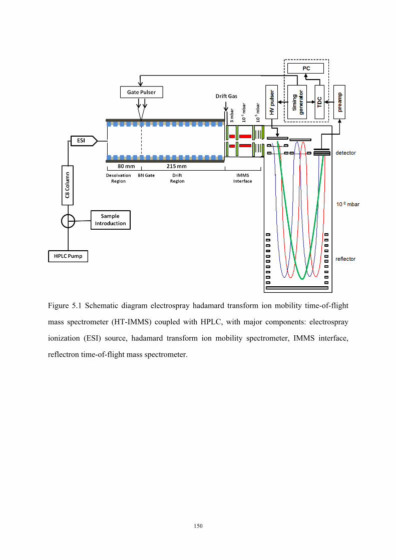
150

Figure 5.1 Schematic diagram electrospray hadamard transform ion mobility time-of-flight

mass spectrometer (HT-IMMS) coupled with HPLC, with major components: electrospray

ionization (ESI) source, hadamard transform ion mobility spectrometer, IMMS interface,

reflectron time-of-flight mass spectrometer.

151

Figure 5.2 IMMS 2-D spectrum of the metabolomes of striatal tissue is displayed in (a), with

x-axis representing m/z (ranges from 100 to 950) and y-axis representing drift time (ranges

from 15 ms to 75ms). The corresponding mass spectrum and ion mobility spectrum are also

152

shown in the figure to illustrate the improvement of 2-D detection when compared with the

1-D spectra. (b) illustrates the global metabolomes of two PFC samples obtained from

repeated saline treated rats with 1-day withdrawal (b1 and b2) and PFC sample obtained from

cocaine treated rats with 1-day withdrawal (b3) using ion mobility spectra.

153

Figure 5.3 PCA score plots of six comparisons: global metabolomes of STR/PFC/NAC

obtained from cocaine treated rats with 1 day withdrawal vs. their corresponding saline

controls, and global metabolomes of STR/PFC/NAC obtained from cocaine

self-administering rats with 3 wks withdrawal vs. their corresponding saline controls. PC-1

and PC-2 represent x-axis and y-axis, and 60% - 80% of the variation is explained in each

score plot.

154

Figure 5.4 Dysregulation of creatine and creatinine in STR/PFC/NAC with 1-day withdrawal.

The magnitudes of the bars represent the average relative intensity value, error bars represent

±SD and asterisk indicates statistical difference (p value < 0.05).

155

Figure 5.5 Intensity profiles of GHS, showing its dysregultaion. The magnitude of the bars

represent the average relative intensity value, error bars represent ±SD and asterisk indicates

statistical difference (p value < 0.05).

156

Figure 5.6 Dysregulation of adenosine in STR/PFC/NAC with 1-day withdrawal and 3-wks

withdrawal. The magnitude of the bars represent the average relative intensity value, error

bars represent ±SD and asterisk indicates statistical difference (p value < 0.05).

157

Chapter 6

Metabolomics of Plasma Fluids from Apolipoprotein AV

Knockout Mice by Hadamard Transform Ambient Pressure Ion

Mobility Time-of-Flight Mass Spectrometry

Abstract

The critical role of apolipoprotein AV (apoAV) in regulating plasma triglyceride level

has been demonstrated but the mechanism remains unresolved. Metabolomics of plasma

fluids from apoAV knockout (KO) mice and wild type (WT) mice under fasted and ad lib fed

dietary treatments was investigated to provide metabolic alternations associated with apoAV.

This is the first comprehensive metabolomics study on apoAV. Hadamard transform ambient

pressure ion mobility time-of-flight mass spectrometry (HT-apIMtofMS) was employed to

perform rapid metabolomics analysis with high resolving power (Rp) separation based on

ion’s size to charge ratio and accurate detection of ion’s mass to charge ratio (m/z). ~1000

metabolite features were detected within 3 minutes, and 40 major metabolite features were

reported and identified based on their accurate m/z values and reduce mobility (K0) values.

Global metabolic analysis by principle component analysis (PCA) on biologically

reproducible metabolite features demonstrated significantly different metabolic patterns for

the four groups of samples. During the specific metabolic analysis, we discovered a “mirror

effect” of dietary treatments on the effect of apoAV on lysophosphatidylcholine related

158

metabolites. Increase of monoacylglyceride class of metabolites caused by the absence of

apoAV was also observed. The separation of glucose and fructose enabled us to monitor the

metabolic alternation of glucose without the interference of its isomer. We found that apoAV

KO subjects have 2-fold increased glucose level when compared with WT, while fructose

level seemed to remain unchanged.

159

6.1 Introduction

Apolipoproteins bind proteins and lipids, playing an important role in lipid and

lipoprotein metabolism. Apolipoprotein AV (ApoAV)1, a 39-kDa protein with 343 residues,

was discovered in 2001 and found to significantly affect plasma triglyceride level with its low

abundance (<1 ug/ml in plasma). The physiological role of apoAV was evaluated by

Pennacchio et al. using transgenic mice that overexpress apoAV protein as well as mice

lacking apoAV2. The 4-fold increased triacylglyceride level in apoAV knockout mice

demonstrated the critical feature of apoAV in modulating plasma lipid homeostasis.

Epidemiological studies further proved that mutations in apoAV have been associated with

hyperglyceridemia3, coronary artery disease4 and type 2 diabetes5 in human and mice.

Knowing that apoAV is located in the apolipoprotein gene cluster in chromosome 11,

and that it’s exclusively synthesized in liver, researchers have successfully developed human

apoAV transgenic mice, allowing specific physiological studies of apoAV. Mechanisms have

been proposed, with regard to its intracellular function of associating with lipid droplets in

the hepatocyte6 and its extracellular function in accelerating the removal of TG-rich

lipoproteins7. More recent investigations associated apoAV with non-alcoholic fatty liver

disease8 and intestinal lipid absorption9. However, the fact that apoAV is present at very low

abundance in plasma leads to the question of its profoundly role in lipid metabolism. The

precise mechanism of apoAV is not completely understood despite the convincing evidence

of its effects. A careful search of the literatures has failed to yield any information linking

160

apoAV with metabolomes other than lipids.

Global metabolomics reveals the identities, quantities of a wide range of diverse

metabolites, providing complementary information to the physiological studies on apoAV.

Metabolomics of plasma has been extensively studied10,11, therefore, the metabolic profiling

as well as the target metabolites including glucose, amino acids, cholesterol and fatty acids

are partly known. The global metabolomics on plasma from apoAV gene modified mice and

wild type (WT) mice monitors the whole metabolome under the designed conditions,

providing metabolic information to reveal more metabolic effects of apoAV in plasma and

enhance our knowledge for understanding the mechanism.

Conventional instrumentations12 used in global metabolomics include nuclear

magnetic resonance (NMR)13, liquid chromatography-mass spectrometry (LC-MS)14 and gas

chromatography-mass spectrometry (GC-MS)15, these methods provide valuable metabolic

information but suffer from either low sensitivity or long analysis time. Hadamard Transform

atmospheric pressure ion mobility time-of-flight mass spectrometry (HT-apIMtofMS)16, a

technique capable of detecting hundreds of metabolites within a few minutes, has been

developed and validated using tissue and fluid extracts.

The general method of ion mobility mass spectrometry (IMMS) has been applied on

various metabolomics studies17-19 and showed its power of sensitive and efficient analysis.

161

Ion mobility spectrometry (IMS) is a rapid gas phase separation technique, originally used for

detecting explosives and drugs. Its capability of differencing ions in millisecond time scale

has made this technique a popular stand-alone system. IMS separation is based on the ion’s

size to charge ratio, making separation of isomers and isobars possible. Ions produced by the

ionization source can quickly attain a constant velocity (νd) under the influences of the

driving force from homogeneous electric field and ion–neutral collisions induced by buffer

gas. Reduced mobility K0 is then derived from νd according to the following equation, can

used to characterize an ion’s identity.

𝐾! = !!

!!! × !"#.!"

! × !

!"#

Where V is the voltage drop across the drift region (length L) of IMS, td is the drift time that

the ion takes to migrate through he drift region, P (in Torr) and T (in Kelvin) are the

operating pressure and temperature.

By coupling IMS to mass spectrometer, the power of separation and detection is

largely increased20. There are several advantages that make IMMS a natural fit for global

metabolomics: 1) rapid pre-MS separation when compared with chromatography methods; 2)

high resolving power IMS separation enabling the differentiation of isomers18; 3) correlation

of mass and mobility (MMCCs) 17,21 providing class identifications not possible by other

methods. Last but not least, HT-apIMtofMS increased the sensitivity by 2 orders of

magnitude when compared with traditional IMMS16, leading to strong responses from the

small amount of plasma samples.

162

The purpose of this work is to apply HT-apIMtofMS to metabolomics on plasma

samples generated from apoAV knockout (KO) mice and WT mice for determining global

and specific metabolic changes associated with apoAV. Moreover, the effects of fasted and

fed on plasma metabolome were also studied in order to associate apoAV with dietary stress.

We believe our work will reveal metabolic effects of apoAV on plasma metabolome, filling

the gap of lacking metabolomics study of apoAV. Meanwhile, the metabolic changes induced

by apoAV and dietary stress could potentially help to understand its mechanism.

163


6.2.1 Subjects and Plasma Collection:

Adult male WT and apo AV KO mice (15-17 months of age) were used. These WT

and apo AV KO mice were bred in house in a facility accredited by the American Association

for the Accreditation of Laboratory Animal Care and were housed with corn cob bedding

under conditions of controlled illumination (12:12-h light-dark cycle, lights from 0600 to

1800). All mice had free access to standard rodent chow (5% fat, Harlan Laboratories,

Indianapolis, IN) and water unless otherwise stated. All procedures were approved by the

University of Cincinnati Institutional Animal Care and Use Committee.

Apo AV KO and WT mice (n = 2 - 4/group) were randomly assigned into four groups.

For fasting group, mice were fasted for 5 h (from 0900 to 1400) with continuous access to

water. Blood samples (120 µL for 50 µL of plasma) for plasma separation were collected into

heparinized capillary tubes from tails. The plasma was separated from whole blood by

centrifugation for 10 minutes (4000 x g). Plasma fluids were frozen at -20°C within one hour

from sampling and stored at -70°C until analyzed.

A total number of 11 plasma samples were analyzed in this study (n = 4 for apoAV

KO mice that were fasted for 5 hrs; n = 3 for apoAV KO mice that were ad lib fed; n = 2 for

WT mice that were fasted for 5 hrs; and n = 2 for WT mice that were ad lib fed).

164

6.2.2 Metabolite Extraction:

An evaluation on the extraction solvent of plasma metabolites for global

metabolomics was conducted using methanol, acetone and acetonitrile. Acetonitrile was

chosen to be the optimal extraction solvent22. Plasma samples were delivered on dry ice and

stored at -80ºC until further use. A volume of 200 µL of iced acetonitrile was added to each

50 µL plasma sample, and vigorously mixed for 2 minutes before stored in 4ºC for overnight

extraction. The samples were centrifuged for 30 min at 13 kRPM, and supernatant containing

extracted metabolites was collected for each sample. ESI solvent comprising a

49.75:49.75:0.5 v/v/v mixture of water, methanol and acetic acid was added into each

supernatant using a 2:1 v/v ratio (ESI solvent: supernatant) for further dilution.

6.2.3 HT-apIMtofMS Analysis:

Prepared samples were introduced for IMMS analysis by electrospray ionization. A

stacked ring IMS was constructed at Washington State University using alternating stainless

steel rings and ceramic rings, where the stainless steel rings were connected by 1 MΩ

resistors. The desolvation region was 8 cm-long and the drift region was 22 cm-long.

Metabolite ions were desolvated in the desolvation region and pulsed into the drift region by

a Bradbury Nielson (BN) ion gate. The HT gate pulsing sequence was generated from

software developed by Tofwerk (AG, Switzerland) and transferred to the BN gate by a gate

pulser made at Washington State University. The smallest gate pulse width was controlled to

180 µs. The IMS was held in ambient pressure (690 – 705 torr) and at 200ºC.

165

The time-of-flight mass spectrometer (tofMS) was coupled to the IMS by an IMMS

interface composing of lenses, nozzles and two segmented quadrupole ion guides. The IMMS

interface provided high transmission efficiency of the ions separated in IMS to tofMS. In this

study, the IMMS analysis was operated under positive mode, and the tofMS was operated in

V-mode with ~5000 – 7000 resolution. A summary of operational details can be found in

Table 6.1 and the schematic picture of the instrument is shown in Figure 6.1a.

During the analysis, 2,6-ditert-butylpyridine was used for internal calibration at a

concentration of 2 µM in all samples. Each sample was analyzed by duplicate runs to ensure

reproducibility. Each IMMS analysis was completed in 3 minutes.

6.2.4 Data Processing:

IMMS data was collected by TofDAQ version 1.92b and processed by IMSviewer

version 1_6d, both developed by Tofwerk (AG, Switzerland). The IMMS data format is

multidimensional, consisting of mass-to-charge ratio (m/z), reduced mobility (K0) and

intensity (counts) for each metabolite feature. Microsoft adaptable peak list for each sample,

as well as all the spectra, were also generated by IMSviewer.

Multivariate analysis approach called principle component analysis (PCA), a

commonly used statistical method for multidimensional data, was employed in this study for

global metabolomics to yield pattern recognition among the 11 samples. PCA was performed

166

on the peak list that merged the biologically reproducible metabolite features from all 11

individual peak lists. Because PCA is an unsupervised method, the analysis was

accomplished without knowing the sample group information. Score plot displayed sample

grouping based on the global metabolic difference contained in the peak lists, and loadings

plot selected metabolite features that significantly affected the pattern recognition. Selected

metabolite features were found to be altered in intensity among different sample groups,

therefore, were considered as potential biomarkers.

Major metabolite features as well as potential biomarkers were identified based on

their exact m/z with mass tolerance of 0.01 and K0 with standard deviation of 2%.

Identifications based on exact m/z were matched with Human Metabolome Database

(HMDB), METLIN Metabolite and Tandem MS Database, and related literatures;

identifications based on K0 were matched with previous studies.

167


6.3.1 IMMS Multidimensional Spectrum:

Similar spectra from duplicate runs demonstrated the reproducibility of IMMS

analysis. The whole metabolome of plasma was displayed in the IMMS 3D plot shown in

Figure 6.1b, which has m/z (ranges from 100 to 900) as x-axis, drift time (ranges from 15 ms

to 75 ms) as y-axis, and intensity as z-axis. The corresponding mass spectrum and ion

mobility spectrum are also included to explain the complexity of the plasma metabolome.

Moreover, with the separation power combine from both IMS and MS, the analysis noise was

reduced and the number of detected metabolite features was increased. There were 900-1000

metabolite features detected with ion counts >10 and ~300 with ion counts >50 after masking

out the background ions. Only major metabolite features that did not vary biologically in all

the plasma samples were used in PCA analysis for pattern recognition.

Table 6.2 summarized the identifications of 40 major metabolite features (ranked by

their intensities) commonly detected in all samples. The accurate m/z and K0 values were

obtained from IMMS analysis; the metabolite identifications including metabolite name,

chemical formula and adduct form, were obtained by matching the m/z and K0 information

with existing databases and previous studies. A wide range of metabolites including amino

acids, carbohydrates, lipids, steroids, and peptides were simultaneously detected,

demonstrating the capability of the 3 minutes IMMS analysis for comprehensive

metabolomics.

168

6.3.2 Global Metabolic Analysis:

Global metabolic alternations were observed in the spectra collected from different

groups of samples. Figure 6.2 contains representative mass spectra and ion mobility spectra

of plasma samples collected from apoAV KO mice fasted for 5 hrs, WT mice fasted for 5 hrs,

apoAV KO mice ad lib fed and WT mice ad lib fed. The mass spectra with m/z ranging from

100 to 900 shared similar major mass peaks, due to the fact that the major metabolite ions

were consistent despite different treatments. In the meanwhile, differences can be observed in

relative intensities for multiple mass peaks. For example, boxed area in the mass spectra was

the m/z region where phospholipids were detected. Decrease in intensity for phospholipids

was observed when comparing fasted apoAV KO mice plasma with fasted WT mice plasma.

In contrast, an increase trend was evident in the ad lib fed mice plasma. In the meanwhile, the

ion mobility spectra collected from the 4 groups of samples showed the same intensity

differences for phospholipids. In general, ion mobility spectra differentiated global metabolic

patterns more easily and clearly when compared with the mass spectra because of the screen

nature of IMS. In practice, it is possible to perform the IMMS analysis of a specific plasma

sample, and identify its classification simply based on its ion mobility spectrum.

Despite observable global metabolic alternation demonstrated by visual inspection of

spectra, further analysis showed the difference statistically. As mentioned earlier, PCA was

performed before knowing the sample group information. Figure 6.3 shows the PCA results

including score plot and loadings plot after assigning the sample group information. Both

169

plots were 2D plots with the first principle component (PC-1) and the second principle

component (PC-2) explaining 45% and 20% of the metabolic variation, respectively. Tight

clustering of WT samples demonstrated good biological reproducibility of WT mice within

the same dietary treatment. However, the grouping of apoAV KO samples was not as tight as

WT samples, indicating more biological variation within the same dietary treatment of

apoAV mice. Despite the existence of biological variance, the score plot still yielded a clear

metabolic pattern that distinguished the four sample groups. Loadings plot, instead of

investigating sample clustering, looked into the metabolite features and determined the ones

that significantly influenced the clustering pattern. Considering outliers as influential

metabolite features, we were able to target seven outliers and identify six of them. Their

identifications were PC (18:0), PC (16:0), PE (16:0), monoradylglycerol (18:0),

phosphocreatinine and choline. As influential metabolites, they were bound to be associated

with either apoAV KO or dietary treatment. PCA allowed visualizing the sample grouping

truly based on the metabolic information, which in this case, was the peak list of metabolite

features generated from IMMS analysis. Therefore, it is evident that both dietary treatment

and apoAV significantly changed plasma metabolome.

6.3.3 Specific Metabolic Alternations:

In order to examine the specific metabolic alternations of the potential biomarkers

selected by PCA loadings plot. ANOVA was used (with 95% confidence interval) to

determine the statistical difference in the relative intensities of a specific metabolite among

170

the four groups of samples. As shown in Figure 6.4 and Figure 6.5, the magnitudes of the

bars represent the average relative intensity values, and the error bars represent ± SD. The

asterisk indicates that statistical difference (p value < 0.05) exited between different sample

groups for the target metabolite. An interesting finding from the loading’s plot and bar graphs

is that the intensities of potential biomarkers (outliers in loading’s plot) changed similarly if

they are near one another in the loading’s plot, examples were shown below.

Lysophospholipids: Figure 6.4 illustrates the metabolic alternations for phospholipid

class of metabolites. In PCA loadings plot, choline and lysophosphatidylcholine (lysoPC)

(16:0) were targeted as potential biomarkers and they appeared in the same area (lower right

corner) in the plot. We found out that they shared the same metabolic alternation trend as

shown in 6.4a. In addition to choline and lysoPC (16:0), more lysoPC metabolites appeared

to have the same alternation trend. The bar graph in 6.4a revealed an increase in the lysoPC

for apoAV KO mice plasma when compared with WT mice plasma under fasted dietary

treatment. However, decrease in intensities of lysoPC metabolites was evident in the KO

mice plasma under the ad lib fed dietary treatment. The above results also matched with the

previous discussions on MS and IMS spectra. The effect of the apoAV protein on plasma

lysoPC level was obvious, however, the effect for subjects under ad lib fed was opposite with

the effect for fasted subjects. This “mirror effect” of dietary treatment on the function of

apoAV protein was firstly discovered and it proved that environment stress such as dietary is

not negligible for the investigation of apoAV.

171

As shown in Figure 6.4b, another two potential biomarkers (lysoPC (18:0) and lyso

PE (16:0)) that appeared to be in the same area (upper right corner) in the loadings plot, also

displayed similar metabolic alternation trend. Different from lysoPC (16:0) and choline, their

intensity changes caused by apoAV was not affected by dietary treatment. Decreased

intensities for the above two biomarkers were discovered for apoAV KO mice plasma when

compared with WT mice plasma. It is well known that lysophospholipid class of compounds

can be involved in lipid signaling by binding protein targets, and their functions in lipid

signaling can be vastly different. This partly explained the difference in alternation trend

displayed in 6.4a and 6.4b. Correlation between apoAV and the biological functions of

lysoPC (18:0) and lyso PE (16:0) could lead to a better understanding of their alteration

trends.

Carbohydrates: As one of the most important metabolites in plasma, glucose was

detected and specifically investigated using bar graph as shown in Figure 6.5a. Its metabolic

alternation was clearly affected by both apoAV and dietary treatment. First of all, it is evident

that the average intensity of glucose was significantly higher in the ad lib fed subjects than

the fasted subjects, indicating that 5 hrs fasting treatment had effectively decreased the

glucose level. Secondly, the glucose level was consistently higher in the apoAV KO subjects

than WT subjects, in both fasted and fed treatments. This result suggested that apoAV

disrupted the metabolic homeostatic of glucose, and lack of apoAV induced the up regulation

of glucose. Therefore, the result supported previous studies indicating that apoAV could be

172

associated with diabetes.

There are many isomers existing as monosaccharides, and glucose is known for the

most common one. To further exam their existence in plasma, we performed selected-mass

mobility analysis on monosaccharide. Figure 6.6 shows the selected-mass mobility spectra of

[C6H12O6+Na]+ (selected m/z = 203.06), with x-axis assigned with drift time (ms) and y-axis

assigned with absolute intensity (counts). The spectra generated from apoAV KO plasma

samples were shown on the top with red trace representing ad lib fed sample and blue trace

representing fasted sample, and the spectra for WT plasma samples were on the bottom. It is

evident that two distinguishable ion mobility peaks under the exact same m/z were observed,

demonstrating the capability of IMMS analysis for distinguishing isomers with high Rp (Rp =

~90 for the early peak and Rp = ~60 for the later peak). To identify these two

monosaccharides, their K0 values were calculated to be 1.53 cm2V-1s-1 for the earlier peak and

1.46 cm2V-1s-1 for the later peak. By matching the K0 values with previous studies on

monosaccharide standards by Dwivedi et al., we were able to identify these two peaks as

[Glucose+Na]+ (K0 = 1.53 cm2V-1s-1), and [Fructose+Na]+ (K0 = 1.46 cm2V-1s-1).

Separation of monosaccharide isomers enabled analysis of the metabolic alternation

for glucose without the interference of its isomers. The absolute intensity values of glucose

indicated a 2-fold increase in plasma caused by the absence of apoAV, and a 3-fold decrease

caused by fasted dietary treatment. Moreover, a close look at the later mobility peak revealed

that the fructose level in plasma was not significantly affected by apoAV, indicating the

173

mechanism of apoAV in affecting “sugar level” might be different for different

monosaccharide compounds.

Monoacylglyceride: MG (18:0) was also selected in PCA as a potential biomarker. Its

metabolic alternation was shown in Figure 6.5b. We found that the alternation trend of MG

(18:0) was similar compared with glucose, demonstrating the similar up regulation caused by

the absence of apoAV and down regulation caused by fasted treatment. Beside MG (18:0),

another two MG metabolites were detected as major peaks in Table 6.2 and they were MG

(16:0) and MG (18:2). As expected, the alternation trend of MG (16:0) and MG (18:2)

matched with MG (18:0), indicating that apoAV decreased the MG level in plasma. With the

previous knowledge of the triglyceride lowering function of apoAV, this finding partly

supported previous investigations because that MG and TG have similarity in both structure

and biological activity. The metabolic change of triglyceride is already known from previous

study and can be more effectively measured in negative ion mode. However, our study was

performed in positive ion mode in order to reveal metabolic changes not yet known.

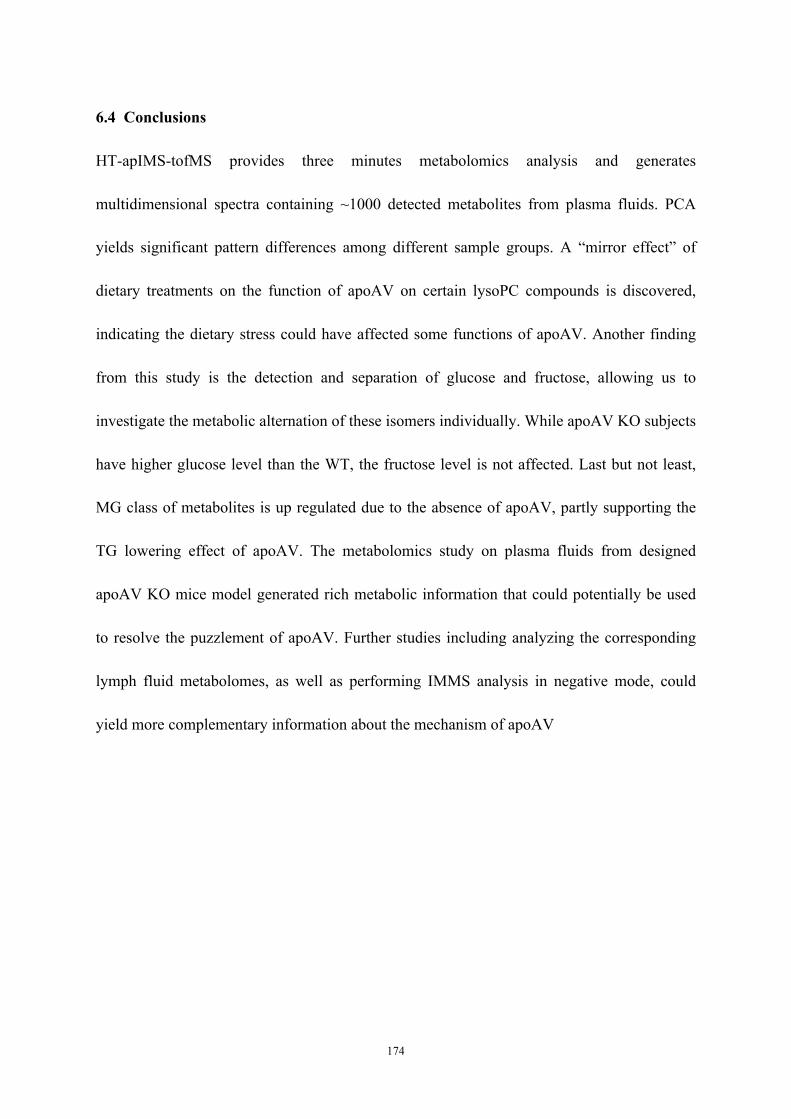
174

6.4 Conclusions

HT-apIMS-tofMS provides three minutes metabolomics analysis and generates

multidimensional spectra containing ~1000 detected metabolites from plasma fluids. PCA

yields significant pattern differences among different sample groups. A “mirror effect” of

dietary treatments on the function of apoAV on certain lysoPC compounds is discovered,

indicating the dietary stress could have affected some functions of apoAV. Another finding

from this study is the detection and separation of glucose and fructose, allowing us to

investigate the metabolic alternation of these isomers individually. While apoAV KO subjects

have higher glucose level than the WT, the fructose level is not affected. Last but not least,

MG class of metabolites is up regulated due to the absence of apoAV, partly supporting the

TG lowering effect of apoAV. The metabolomics study on plasma fluids from designed

apoAV KO mice model generated rich metabolic information that could potentially be used

to resolve the puzzlement of apoAV. Further studies including analyzing the corresponding

lymph fluid metabolomes, as well as performing IMMS analysis in negative mode, could

yield more complementary information about the mechanism of apoAV

175

Reference

(1) Beckstead, J. A.; Oda, M. N.; Martin, D. D. O.; Forte, T. M.; Bielicki, J. K.;

Berger, T.; Luty, R.; Kay, C. M.; Ryan, R. O. Biochemistry 2003, 42, 9416–9423.

(2) Pennacchio, L. A. Science 2001, 294, 169–173.

(3) Priore Oliva, C.; Pisciotta, L.; Li Volti, G.; Sambataro, M. P.; Cantafora, A.;

Bellocchio, A.; Catapano, A.; Tarugi, P.; Bertolini, S.; Calandra, S. Arterioscler

Thromb Vasc Biol 2005, 25, 411–417.

(4) Vaessen, S. F. C.; Schaap, F. G.; Kuivenhoven, J.-A.; Groen, A. K.; Hutten, B.

A.; Boekholdt, S. M.; Hattori, H.; Sandhu, M. S.; Bingham, S. A.; Luben, R.; Palmen,

J. A.; Wareham, N. J.; Humphries, S. E.; Kastelein, J. J. P.; Talmud, P. J.; Khaw,

K.-T. The Journal of Lipid Research 2006, 47, 2064–2070.

(5) Talmud, P. J.; Cooper, J. A.; Hattori, H.; Miller, I. P.; Miller, G. J.; Humphries,

S. E. Diabetologia 2006, 49, 2337–2340.

(6) Shu, X.; Chan, J.; Ryan, R. O.; Forte, T. M. The Journal of Lipid Research 2007,

48, 1445–1450.

(7) Merkel, M. Journal of Biological Chemistry 2005, 280, 21553–21560.

(8) Sharma, V.; Ryan, R. O.; Forte, T. M. … et Biophysica Acta (BBA)-Molecular

and … 2012.

(9) Yoshino, Y.; Okada, T.; Abe, Y.; Odaka, M.; Kuromori, Y.; Yonezawa, R.;

Iwata, F.; Mugishima, H. Obesity Research & Clinical Practice 2013, 7, e415–e419.

(10) Li, W.; Tse, F. L. S. Biomed. Chromatogr. 24, 49–65.

176

(11) Bruce, S. J.; Jonsson, P.; Antti, H.; Cloarec, O.; Trygg, J.; Marklund, S. L.;

Moritz, T. Analytical Biochemistry 2008, 372, 237–249.

(12) Dunn, W. B.; Ellis, D. I. TrAC Trends in Analytical Chemistry 2005, 24, 285–

294.

(13)Hu, Z.; Deng, Y.; Hu, C.; Deng, P.; Bu, Q.; Yan, G.; Zhou, J.; Shao, X.; Zhao, J.;

Li, Y.; Zhu, R.; Xu, Y.; Zhao, Y.; Cen, X. Behavioural Brain Research 2012, 231,

11–19.

(14) Lu, W.; Bennett, B. D.; Rabinowitz, J. D. Journal of Chromatography B 2008,

871, 236–242.

(15) Koek, M. M.; Muilwijk, B.; van der Werf, M. J.; Hankemeier, T. Anal. Chem.

2006, 78, 1272–1281.


Chem. 2014, 86, 1661–1670.

(17) Kaplan, K.; Dwivedi, P.; Davidson, S.; Yang, Q.; Tso, P.; Siems, W.; Hill, H. H.,

Jr. Anal. Chem. 2009, 81, 7944–7953.

(18) Lapthorn, C.; Pullen, F.; Chowdhry, B. Z. Mass Spectrom. Rev. 2012, 32, 43–

71.

(19) Armenta, S.; Alcala, M.; Blanco, M. Analytica Chimica Acta 2011, 703, 114–

123.

(20) Kanu, A. B.; Dwivedi, P.; Tam, M.; Matz, L.; Hill, H. H., Jr. J. Mass Spectrom.

2008, 43, 1–22.

177

(21) Fenn, L. S.; Kliman, M.; Mahsut, A.; Zhao, S. R.; McLean, J. A. Anal Bioanal

Chem 2009, 394, 235–244.

(22) Bruce, S. J.; Tavazzi, I.; Parisod, V.; Rezzi, S.; Kochhar, S.; Guy, P. A. Anal.

Chem. 2009, 81, 3285–3296.

178

Table 6.1 Summary of experimental details.

Parameters Details ESI needle bias voltage 3000 V

Sample flow rate 3 ul/min Voltage on the ion gate 7170 V

Electric field 303 V/cm 1st segmented quadruole pressure 3 mbar 2nd segmented quadruole pressure 1 × 10-2 mbar

tofMS chamber pressure 3.8 × 10-7 mbar

179

Table 6.2 Summary of the identifications of the first 40 major metabolite features detected in

all 11 samples. The exact m/z and K0 (cm2V-1s-1) were measured in IMMS analysis, and the

identifications were matched with existing databases.

Number m/z K0 Metabolite Chemical Fomula Adduct

1 104.12 1.97 Choline C5H14NO [M]+

2 111.96 1.53 Methyl isothiocyanate C2H3NS [M+K]+

3 114.96 1.53 Thioacetate C2H3OS [M+K]+

4 155.99 1.54 Homocysteine thiolactone C4H7NOS [[M+K]+

5 157.09 1.67 N/A N/A N/A

6 174.99 1.52 Oxidized dithiothreitol C4H8O2S2 [M+Na]+

7 197.01 1.54 Aconitic acid C6H6O6 [M+Na]+

8 199.01 1.56 Ascorbic acid C6H8O6 [M+Na]+

9 203.06 1.54 Glucose C6H12O6 [M+Na]+

10 204.13 1.48 Acetylcarnitine C8H17N3O3 [M+H]+

11 211.00 1.42 p-Cresol sulfate C7H8O4S [M+Na]+

12 216.01 1.53 Phosphocreatinine C4H8N3O4P [M+Na]+

13 235.02 1.51 5-Carboxyvanillic acid C9H8O6 [M+Na]+

14 250.18 1.27 N/A N/A N/A

15 252.03 1.42 Phosphoribosylamine C5H12NO7P [M+Na]+

16 296.15 1.32 Gly Val Val C12H23N3O4 [M+Na]+

17 313.28 1.00 LysoPE(16:0) C21H44NO7P [M+H-141]+

18 341.31 0.95 LysoPC(18:0) C26H54NO7P [M+H-182]+

19 353.27 0.97 MG(16:0) C19H38O4 [M+Na]+

20 377.25 1.01 MG(18:2) C21H38O4 [M+Na]+

21 381.29 0.92 MG(18:0) C21H42O4 [M+Na]+

22 401.33 0.93 5,6-trans-25-Hydroxyvitamin D3 C27H44O2 [M+H]+

23 437.18 0.96 Ala Met Cys Leu C17H32N4O5S2 [M+H]+

24 445.21 0.89 Asp Thr Ile Pro C19H32N4O8 [M+H]+

25 473.24 0.85 Lys Tyr Tyr C24H32N4O6 [M+H]+

26 496.32 0.79 LysoPC(16:0) C24H50NO7P [M+H]+

27 518.30 0.78 LysoPC(16:0) C24H50NO7P [M+Na]+

28 520.32 0.80 LysoPC(18:2) C26H50NO7P [M+H]+

29 522.33 0.78 LysoPC(18:1) C26H52NO7P [M+H]+

30 524.34 0.76 LysoPC(18:0) C26H54NO7P [M+H]+

31 534.28 0.77 PS(17:0) C23H46NO9P [M+Na]+

32 542.30 0.79 LysoPC(20:5) C28H48NO7P [M+H]+

33 544.31 0.77 LysoPC(20:4) C28H46NO7P [M+H]+

34 566.30 0.78 LysoPC(20:4) C28H50NO7P [M+Na]+

35 568.31 0.77 LysoPC(20:3) C28H52NO7P [M+Na]+

180

36 590.29 0.77 Arg Met His Phe C26H39N9O5S [M+H]+

37 659.25 0.66 Gln Trp Tyr Tyr C34H38N6O8 [M+H]+

38 780.47 0.59 PS(36:6) C42H70NO10P [M+H]+

39 806.47 0.59 PS(38:7) C44H72NO10P [M+H]+

40 828.46 0.58 PS(40:10) C46H70NO10P [M+H]+

181

Figure 6.1 (a) Schematic diagram of electrospray ionization coupled with hadamard

transform ambient pressure ion mobility time-of-flight mass spectrometry. The ion mobility

spectrometer was coupled with the mass spectrometer by a quadrupole IMMS interface. (b)

Illustrative IMMS 3D spectrum with m/z (100 - 900) as x-axis, drift time (15ms – 75ms) as

y-axis, and intensity as z-axis. The extracted mass spectrum and ion mobility spectrum were

shown on the right.

182

Figure 6.2 Representative mass spectra (top) and ion mobility spectra (bottom) for four

different groups of samples, including plasma fluids from apoAV KO mice fasted for 5 hrs,

WT mice fasted for 5 hrs, apoAV KO mice ad lib fed and WT mice ad lib fed. Mass spectra

have x-axis assigned with m/z (100 - 900) and ion mobility spectra have x-axis assigned with

183

drift time (15ms- 75ms). Both spectra have y-axis as relative intensity. Different patterns can

be observed from the spectra. Areas circled with blue boxes represent the m/z (drift time)

range where the lysophospholipid class of compounds was detected.

184

Figure 6.3 PCA results including score plot (top) and loadings plot (bottom). The first

principle component explained 45% of the variance among 11 samples, and the second

principle component explained 20% of the variance. Clear sample grouping patterns can be

observed in score plot and metabolite features located away from the center of loadings’ plot

were selected as potential biomarkers.

185

Figure 6.4 Specific metabolic alternations for lysophospholipid class of metabolites. (a)

shows the intensity profiles for five metabolites that share the similar metabolic alternation,

and (b) shows the intensity profiles for another two lysophospholipid metabolites displaying

different alternation compared with (4). In both Figure 6.4 and 6.5, error bars represent ±SD

and asterisk indicates statistical difference (p value < 0.05).

186

Figure 6.5 Intensity profiles for glucose (a) and MG (18:0) (b) for four groups of samples.

187

Figure 6.6 Selected-mass ion mobility spectra for monosaccharide ion (m/z = 203.06). Ion

mobility spectra extracted from apoAV KO samples were listed on top with blue trace

representing fasted sample and red trace representing ad lib fed sample. Bottom spectra were

extracted from WT samples. Two ion mobility peaks were observed and identified

[Glucose+Na]+ with K0 = 1.53 cm2V-1s-1 and [Fructose+Na]+ with K0 = 1.46 cm2V-1s-1.

188

Chapter 7

Conclusions

I. Overall Conclusion

Complex mixture analysis has been a great challenge on for analytical chemistry.

Metabolome, as an example of a complex mixture, was specifically investigated in this work

using metabolomics by ion mobility mass spectrometry (IMMS). IMMS showed great

potential for the comprehensive analysis of complex samples with two-dimensional

separation, high sensitivity and enhanced capability for structure elucidation. This work

implemented the hadamard transform multiplexing technique and its related data processing

for metabolomics.

The unique advantages provided by IMMS allow sensitive and comprehensive

metabolomics analysis with the following capabilities: 1) high throughput analyses; 2) easy

coupling with chromatographic separation instruments to achieve a wider detection range; 3)

rapid isomer separation; 4) measurement of collision cross section (Ω) values; 5) isotopic

ratio analysis for metabolite identifications; 6) mobility-mass correlation curves (MMCCs)

for class identifications.

189

II. Specific Conclusions

The metabolomics study in Chapter 2 demonstrated the application of conventional

drift tube ion mobility mass spectrometry for the metabolic analysis of Parkinson’s

disease-like (PD-like) rat striatal tissues. PCA was use as the primary statistical analysis and

displayed significant patterns between PD-like samples and healthy controls. The high IMS

resolving power enabled separation between dopamine and its isomer (proposed structure

2-(2,4-dihydroxylphenyl) ethylamine). The co-existence of these two compounds in healthy

control samples along with the absence of dopamine in PD-like samples demonstrated that

the reduction of dopamine in PD might be underestimated. Potential biomarkers were

selected using the same PCA model, and identified as cholesterol, vitamin B3, lactaldehyde

and amino acids.

The metabolomics study in Chapter 2 employed the conventional pulse mode IMMS

that had a limited duty cycle (0.25%). Therefore, the IMMS analysis time was between 15 –

20 minutes. In order to improve the duty cycle, Chapter 3 employed multiplexing technique

by superimposing hadamard transform (HT) sequence on the ion gate. We obtained ~200

times improvement of duty cycle while retaining high IMS resolving power. The

performance of HT-IMMS was assessed using metabolite standard mixture at a wide

concentration range, and the limit of detection in HT-mode was demonstrated to be ~10 times

lower than conventional pulse mode. NIST Standard Reference Material 1950 Metabolites in

Human Plasma was also analyzed in both modes with more metabolite features detected in

190

HT mode when compared with pulse mode. In order to increase the response of complex

mixture analysis, rapid chromatographic separation prior to IMMS analysis was also

evaluated using a striatal tissue sample. It was evident that the ionization suppression caused

by direct infusion was largely reduced, and more metabolite features were observed in high

m/z region (m/z >800). Therefore, IMMS technique coupled with HT sequence and prior

chromatographic separation was developed and evaluated, allowing metabolomics analysis

within 2 – 3 minutes with high sensitivity.

The study shown in Chapter 4 was the first application of HT-IMMS on

metabolomics, which specifically investigated the metabolomes of human blood. The focus

of this work was to apply the unique merit of HT-IMMS to help metabolomics analysis and

metabolite identifications. Multiple approaches were applied including accurate isotopic ratio

analysis, isomer/isobar separations, charge states separation and mobility-mass correlation

curves classifications. We were able to identify 185 metabolite features after de-isotope using

the exact mass information and unique structural information provided by IMMS. Among the

185 metabolite features, five pairs of isomers and isobars were separated and assigned with

identifications. Moreover, five MMCCs with good linearity were observed and they provided

qualitative information regarding to compound classifications. HT-IMMS provided

comprehensive metabolomics analysis of blood samples within 3 minutes with

multidimensional information generated, demonstrating HT-IMMS as a natural fit for

metabolomics and metabolite identifications.

191

To further extend the applications of HT-IMMS to metabolomics, Chapter 5 described

a neuronal metabolic study, revealing the global and specific neuronal metabolic changes

caused by cocaine self-administration followed by 1 day or 3 weeks withdrawal. With regard

to analytical platform, this study employed chromatographic separation prior to HT-IMMS

analysis and achieved good metabolite response and wide detection range. With regard to

data processing, we improved the biomarker selection model from Chapter 2, and used both

multivariate analysis (PCA) and univariate analysis approaches to target potential biomarkers,

generating a complete profile of metabolic changes induced by cocaine self-administration.

Among the selected potential biomarkers, oxidative stress and energy related metabolites

were specifically investigated. The dyregulation of creatine, creatinine, adenosine and

glutathione matched with previous studies and demonstrated the brain regionally specific

metabolic changes. In general, these findings supported the multi-event mechanism of

cocaine abuse.

Work in extending metabolomics applications was continued in Chapter 6, where the

metabolic function of apolipoprotein AV (apoAV) was investigated using the plasma fluids

collected from apoAV knockout mice and wild type mice under fasted and ad lib fed dietary

treatments. Different metabolic patterns were noted for different sample groups after PCA,

and the biomarkers selected by PCA were extended to their corresponding classes including

lysophosphatidycholine, monoacylglyceride and carbohydrate. A “mirror effect” of dietary

192

treatments on the effect of apoAV on lysophosphatidylcholine related metabolites was

observed, and the increase of monoacyglyceride class of metabolites was noted in the apoAV

KO samples for both dietary treatments. In addition, high resolving power of IMS allowed

separation between glucose and fructose, providing specific metabolic changes without the

interference of each other. It was conclude that the absence of apoAV caused 2-fold increase

in glucose level, while appeared to have little to no influence on fructose level.

Data processing using statistical approach was an important part in Chapter 2, Chapter

5, and Chapter 6. And it was concluded that there’s no standardized procedure for statistical

analysis of metabolomics. Appendix provided the optimized comprehensive data processing

procedure for IMMS type of data, including the estimation of censored values (also known as

missing values), multivariate analysis, univariate analysis and cluster analysis. Censored

values were estimated using distribution analysis by Minitab, enabling us to keep metabolic

information intact. Univariate analysis was optimized using adjusted t-test in linear models

for microarray data (limma), which selected the “real” significant changes using adjusted

variance instead of metabolite feature variance. This univariate analysis approach generated a

fewer number of significant changes when compared to the conventional t-test, allowing us to

focus on a fewer number of biomarkers. Finally, cluster analysis was employed to analyze the

selected biomarkers, providing insights in metabolic pathways.

Chapter 2 showed an example of metabolomics study on PD-like striatal tissue using

193

conventional IMMS approach, advanced in high resolving power but limited in throughput.

The work in Chapter 3 evaluated HT-IMMS by a number of metabolite standards and various

types of complex mixtures, proving the 2 orders of magnitude increase in sensitivity while

maintaining high resolving power. The application study in Chapter 4 illustrated the unique

merit of HT-IMMS in global metabolomics and metabolite identifications. Based on the

above improvements, applications were extended to global metabolic study on cocaine abuse

and apoAV in Chapter 5 and Chapter 6, respectively. The findings in the dysregulation of

potential biomarkers and proposed metabolic pathways may provide complementary

information to the pathological studies. The optimization in data processing was further

addressed in Appendix, illustrating the critical role of statistical analysis in global

metabolomics. With the continued development in HT-IMMS techniques and optimization in

data processing, a multitude of applications should be extended, not only for metabolomics,

but also for all types of complex mixture analyses.

194

Appendix A

Statistical Analysis for Metabolomics using Multivariate

and Univariate Approaches

Introduction

Metabolomic1,2, an important part of integrate “omics”, is the downstream of

genomics and proteomics. Specifically, metabolomics is the scientific study by profiling and

measuring thousands of metabolites. The result of metabolomics represents the collection of

all metabolites in a cell, tissue, or organ. Metabolites are the end products of cellular

processes, including amino acids, glucose, cholesterols, lipids and peptides. And their levels

can be regard as the ultimate response of biological systems. There are a few particular

purposes of metabolomics study. The first aim is to differentiate metabolic states/pattern

recognition, for example, healthy state vs. disease state, early disease state vs. late disease

state. And the second one is to find biomarkers3 that can be used for diagnosis or cure. These

biomarkers refer to the variables that change significantly among different metabolic states,

and can often times be related to the disease mechanism with certain biological functions.

The third one aims to yield significant biological insights by correlating the targeted

biomarkers4 with other variables/metabolites, therefore, generate certain metabolic pathways

that can further be related to proteomics and genomics.

195

Common to all analytical methods5 for metabolomics is that they all produce a

massive amount of data, impossible to be handled completely manually and without the use

of statistics. The number of variables (also called metabolite features) can be hundreds or

even thousands, much larger than the number of experiments (usually 3-20); therefore the

metabolomics data are high dimensional. This situation has made multivariate statistics a

natural fit because that it works well with “long and lean” data sets in general scope.

Multivariate statistics includes dimension reduction methods such as principle component

analysis, partial least square analysis, and linear discriminate analysis. Such multivariate

approaches are also robust to random variation and experimental error.

Nowadays, nuclear magnetic resonance (NMR)6 and mass spectrometry (MS)7 are

two predominant platforms utilized in metabolomics, and both methods perform

metabolomics analysis by detecting the chemical formula and molecular structure of

metabolite ions. MS-based technique is preferred by its high sensitivity, low cost and

straightforward data format. The basis of MS technique is to measure the metabolite ion’s

mass (also called molecular weight). However, due to the complex nature of metabolomics,

pre-separation is often times required before MS analysis for a wider detection range. The

pre-separation step not only increases the number of detectable metabolite features, but also

provides another dimension of information regarding to the structure of the metabolite. Ion

mobility spectrometry (IMS)8 is one of the popular pre-separation techniques and has been

widely applied to metabolomics. IMS separate metabolite ions based on their size, and when

196

coupled with MS technique, ion mobility mass spectrometry (IMMS) can generate

multidimensional information for each metabolite feature.

MS generates a mass to charge ratio (mz) for each metabolite feature, while IMS

generates mobility value (K0) related to ionic size. They can be combined as mzK0 feature9,

which is utilized for charactering each metabolite feature. Every mzK0 feature is also

assigned with an intensity value, which represents the concentration of the corresponding

metabolite feature in a particular sample. The final metabolomics data set for a certain sample

contains hundreds of mzKo features with assigned intensity values. When multiple data sets

generated for multiple samples, one can combine these data sets by merging mzKo features,

and in the end, a complex data matrix presents.

Even though the analytical approach is efficient and reproducible, there are

difficulties along with the data processing using appropriate statistical analysis. Unlike

genomics data and proteomics data, the metabolomics data is more versatile and

hard-to-predict10. Among the statistical approaches utilized in metabolomics, there’s still no

defined standard procedure, therefore, challenges and concerns appeared during recent years.

The major challenges are how to select biomarkers from the massive data matrix, and how to

relate these biomarkers with other metabolites to form a metabolic pathway. This “fishing”

procedure is critical and needs to be handled with caution.

197

The general steps involved in the statistical analysis of metabolomics are usually

followed as data pre-treatment11 (including raw data normalization and mzKo feature

merging), exploratory analysis (e.g. principle component analysis (PCA)12 and partial least

square-discriminant analysis (PLS-DA)13). The exploratory analysis is developed to distill the

large amounts of data by reducing the dimensionality of the raw data set. The result can

elucidate the relations between samples and their classification. For example, by utilizing

PCA, it can simplify large datasets into a new coordinate system (components), and these

new components are derived from the original data in such a way that the greatest variation in

the date is captured in the first group (first component PC1), the second greatest variation in

the second (PC2) and so on. This method of viewing large amounts of data in a simplified

manner provides scientists a means to visualize and detect variations between sample groups.

PCA loadings’ plot shows where the components found their variation and thereby which

metabolites have affected in the relations and groupings. Therefore, potential biomarkers are

defined as the metabolite features that significantly affected the relations. The above example

shows the general approach of statistical analysis on metabolomics type of data, and it indeed

effectively accomplished the global pattern recognition, and also selected some potential

biomarkers for the second aim.

However, improvements are still needed at each stage of data processing, and there

are a few problems/concerns that have been overlooked. One of them is how to appropriately

deal with censored data generated during the analytical experiment. Due to the biological

198

variation among samples and the limit of detection (also called threshold) for the analytical

technique, censored data can appear among biological replicates. It is possible that certain

metabolite features can be detected in the first and second replicates, but not in the third one.

When encountered with this situation, researchers often times mask out metabolite features

that have censored data. However, this is clearly not the ideal solution since the discarded

metabolite features could be important in biological sense. Another problem is biomarker

selection. As described earlier, multivariate statistical models can generate certain biomarkers

with regard to their contribution in pattern recognition. However, the selection procedure was

based on variance, which can be dominated by metabolite features that have high intensity

values. Under this situation, the contribution of metabolite features that have small intensity

values can often times be underestimated or even ignored. The third challenge in

metabolomics is how to relate the selected biomarkers with metabolic pathways, and till

today, this procedure has been realized fully dependent on the biological knowledge.

With the gaps described above as the aims of this study, we developed new data

processing algorithm using Minitab and R. By re-processing the raw data using distribution

analysis on left-censoring data, we were able to avoid discarding information. And by

applying univariate analysis14 on all metabolite features, more potential biomarkers were

selected including the ones with small intensity values. Moreover, cluster analysis was

performed on the selected biomarkers, in order to sort the metabolic pathways from statistical

prospective.

199

Experiments

Sample Preparation:

Six male Sprague Dawley rats were obtained from Washington State University

breeding colony and were housed two or three per cage in a university vivarium with a 12-h

light/dark cycle, at 22 to 24 °C, and with ad libitum access to food and water. Animal

procedures were in strict accordance with the NIH Guide for the Care and Use of Laboratory

Animals and were approved by the University Animal Care Committee15. Three animals were

used as saline-treated controls, and three were given an acute dose of cocaine at 30 mg/kg i.p.

45 min every day until maximal locomotor activity was achieved (cocaine addicted). Rats

were given 24 hr withdrawal after the last dose of drug/saline before decapitated and their

brain dissected on an ice-cold watch glass with an ice-cold razor blade. Left and right striatal

samples were pooled from each rat, and stored on dry ice. Samples were weighed and

individually transferred to a sample container where the sample was sonicated in 500 µL of

electrospray solution made up with 50:50 methanol/water, to extract metabolites. Denatured

proteins and cellular debris were separated by centrifugation for 10 min in a desktop

centrifuge. The supernatant was collected and stored in -80°C before analyzed.

Ion Mobility Mass Spectrometry (IMMS) Analysis and Data Format:

Electrospray ionization was applied on the supernatant to ionize the metabolite

molecules into metabolite ions. IMMS analysis lasted for 5 minutes for each sample with a

sample flow rate of 3 ul/min. Multidimensional information was exported and organized for

200

each sample using mzKo representing metabolite features, and intensity values were assigned

to complete one data set. When six data sets were generated, mzKo features were merged into

one data set with all information included.

Table 1 is part of the merged data set, illustrating the data format. As shown in the

table, the data set contains 6 columns with each column corresponding to each sample, and

~150 rows with each row corresponding to each metabolite feature, the number in each cell

represents the intensity value of the corresponding metabolite feature in the corresponding

sample. The samples were named as STR C1, C2, C3 (representing cocaine abused samples)

and S1, S2, S3 (representing saline controls). It is important to note that there are a few cells

with 0 intensity value, which actually indicate the left censoring data not detected by IMMS.

201

Statistical Analysis Results

Evaluate Left-censoring Data using Distribution Analysis:

The prediction of left-censoring data undoubtedly assigned more reasonable intensity

value compared to simply using 0 or discarding the metabolite feature. In this study, we used

the distribution analysis function in Minitab. By setting the instrument analysis threshold at

50, the distribution was selected with the most linear probability plot and the distribution

parameters were estimated by MLE. The prediction of left-censoring data was then

determined by estimating percentiles for certain percent (determined by the number ratio of

left-censoring metabolite features and total metabolite features). The results were shown in

Table 2, with all left-censoring data replaced with the prediction values. To be more specific,

Weibull distribution was found to have the most linear probability, and the left-censoring data

for STR C1, C2, C3, S1, S2, S3 were replaced with predicted values 46, 53, 53, 67, 69, 59,

respectively.

Statistical Analysis using Multivariate Approach:

Principle component analysis (PCA) was utilized as dimension reduction approach

after normalization the raw data and replacing left-censoring data with prediction values. The

unsupervised nature of PCA enables it for pattern recognition by score plot and biomarker

selection by loadings’ plot. PCA was performed using Table 2, and PCA results were shown

in Figure 1 with both score plot and loading’s plot. As shown in the score plot, cocaine

samples (circled in red) are well separated from the saline controls (circled in green). The

202

loadings’ plot has a few outliers representing the metabolite features significantly affected the

pattern recognition. These outliers were extracted further explained by cluster analysis.

Selection of Biomarkers using Univariate Approach:

Unpaired t-test was used initially to obtain biomarkers in addition to the biomarkers

generated from PCA. However, it yielded 31 metabolite features with P-value less than 0.05.

Large amount of potential biomarkers can make the later analysis very difficult because that

each metabolite feature considered as potential biomarker has to be verified, identified and

understood. The adjusted t-test in linear models for microarray data (limma) resolved this

problem by reducing the number of significant features using adjusted variance. The rationale

for adjusted t-test is the fact that the sample variance is not an efficient statistics due to the

small number of observations (3 in this study), and adjusted t-test computes an expected

variance and adjusts the observed ones towards this expected value. By computing the

P-value from adjusted t-test, the number of metabolite features with significant P-value was

effectively reduced to 7. Table 3 contains top 20 metabolite features (ranked by P-value),

showing the significant improvement from adjusted t-test.

Cluster Analysis on Biomarkers for pathway Identification:

The purpose of cluster analysis is to sort metabolite features into respective categories

in a way that the degree of association between metabolite features is maximal if they belong

to the same group and minimal otherwise. Hierarchical clustering analysis was applied on 12

203

metabolite features selected as biomarkers (7 with significant P-values from the adjust t-test,

5 were identified as outliers from PCA), and result was displayed in Figure 2. It shows that

two metabolite features with mzKo 104.10:1.96 and 268.11:1.34 fell into the same category.

These two metabolite features were identified as Choline and Adenosine, which were both

involved in the energy metabolism in a system of biology, proving the feasibility of cluster

analysis.

204

Conclusions

Metabolomics data generated from global metabolomics analysis contains large

amount of information, and often times has more metabolite features than sample size.

Metabolite features characterized by m/z and Ko were obtained from ion mobility mass

spectrometry analysis in a cocaine-abused rats study, and statistical approaches were

developed for pre-processing, pattern recognition and biomarkers selection. Left-censoring

data was evaluated and predicted using distribution analysis. Principle component analysis

was employed as a dimensional reduction method with pattern recognition yielded for

cocaine abused samples and saline control samples. Moreover, it generated 5 verified outliers

(identified as biomarkers) from the loadings’ plot. Univariate analysis approaches were also

evaluated for more biomarkers selection. Plain unpaired t-test was applied with 31 significant

biomarkers appeared to be significant. The number of biomarkers was reduced to 7 by

applying adjusted t-test in linear models for microarray data. Clustering the biomarkers based

their degree of association has further helped for metabolic pathways analysis, which lead to

the final goal of metabolomics study.

205

Reference

(1) Creek, D. J.; Jankevics, A.; Breitling, R.; Watson, D. G.; Barrett, M. P.; Burgess, K.

E. V. Anal. Chem. 2011, 83, 8703–8710.

(2) Bruce, S. J.; Jonsson, P.; Antti, H.; Cloarec, O.; Trygg, J.; Marklund, S. L.; Moritz, T.

Analytical Biochemistry 2008, 372, 237–249.

(3) Griffiths, W. J.; Koal, T.; Wang, Y.; Kohl, M.; Enot, D. P.; Deigner, H. P. Angew.

Chem. Int. Ed. 2010, 49, 5426–5445.

(4) Smith, R. D. Clinical Chemistry 2012, 58, 528–530.


(6) Aranı bar, N.; Ott, K.-H.; Roongta, V.; Mueller, L. Analytical Biochemistry 2006,

355, 62–70.

(7) Katajamaa, M.; Orešič, M. Journal of Chromatography A 2007, 1158, 318–328.


43, 1–22.

(9) Smith, C. A.; Want, E. J.; O'Maille, G.; Abagyan, R.; Siuzdak, G. Anal. Chem. 2006,

78, 779–787.

(10) Issaq, H. J.; Van, Q. N.; Waybright, T. J.; Muschik, G. M.; Veenstra, T. D. J. Sep.

Science 2009, 32, 2183–2199.

(11) Bijlsma, S.; Bobeldijk, I.; Verheij, E. R.; Ramaker, R.; Kochhar, S.; Macdonald, I. A.;

van Ommen, B.; Smilde, A. K. Anal. Chem. 2006, 78, 567–574.

(12) Pan, Z.; Gu, H.; Talaty, N.; Chen, H.; Shanaiah, N.; Hainline, B. E.; Cooks, R. G.;

206

Raftery, D. Anal Bioanal Chem 2006, 387, 539–549.

(13) Karp, N. A.; Griffin, J. L.; Lilley, K. S. Proteomics 2005, 5, 81–90.

(14) Vinaixa, M.; Samino, S.; Saez, I.; Duran, J.; Guinovart, J. J. Metabolites 2012.

(15) Kaplan, K. A.; Chiu, V. M.; Lukus, P. A.; Zhang, X.; Siems, W. F.; Schenk, J. O.;

Hill, H. H. Anal Bioanal Chem 2013, 405, 1959–1968.

207

Figure A1: PCA results including Score plot and Loadings’ plot, with 62% of variance

explained.

208

Figure A2: Hierarchical Clustering analysis result on 12 biomarkers.

130.05:1.72

114.06:1.86

176.05:1.61

137.05:1.75

104.07:1.96

162.11:1.63

761.60:0.59

798.55:0.58

142.03:1.73

127.06:1.84

104.10:1.96

268.11:1.34

010000

20000

30000

40000

50000

Cluster Dendrogram

hclust (*, "complete")d

Height

209

Table A1: Part of the raw data set generated from IMMS experiments, illustrating the data

format.

m/z: K0 STR C1 STR C2 STR C3 STR S1 STR S2 STR S3

104.06:1.91 4862 1995 1643 2384 3126 3556

104.10:1.96 8904 11503 7191 10561 12288 19962

105.10:1.96 577 889 528 773 1016 1493

106.04:1.75 357 193 206 466 429 290

112.89:1.95 79 154 0 131 141 235

114.06:1.89 13095 4243 9165 9101 7269 6781

115.06:1.88 1064 517 616 684 560 575

119.03:1.34 553 515 0 456 472 173

120.06:1.80 279 0 0 429 478 376

123.05:1.80 3349 1840 3359 2845 2947 2714

124.04:1.80 541 388 10 1006 0 442

127.06:1.84 546 514 373 0 0 0

129.06:1.80 732 536 980 852 511 557

210

Table A2: Result of censored value estimation, “0” values were replaced by estimations.

m/z: Ko STR C1 STR C2 STR C3 STR S1 STR S2 STR S3

80.04:2.08 608 727 53 1874 927 1234

84.07:1.69 375 53 123 310 163 59

86.05:1.87 6857 9880 4874 4218 3408 4367

87.05:1.92 551 544 53 444 592 419

90.05:1.79 389 452 463 405 623 308

90.08:2.08 5185 4372 4558 3195 2921 1657

90.50:1.96 210 53 166 278 288 67

91.05:1.76 205 214 335 67 69 59

91.09:2.08 304 188 199 227 121 113

99.05:1.81 492 53 851 502 238 59

104.06:1.91 4862 1995 1643 2384 3126 3556

104.10:1.96 8904 11503 7191 10561 12288 19962

105.10:1.96 577 889 528 773 1016 1493

106.04:1.75 357 193 206 466 429 290

112.89:1.95 79 154 53 131 141 235

114.06:1.89 13095 4243 9165 9101 7269 6781

115.06:1.88 1064 517 616 684 560 575

119.03:1.34 553 515 53 456 472 173

120.06:1.80 279 53 53 429 478 376

123.05:1.80 3349 1840 3359 2845 2947 2714

124.04:1.80 541 388 53 1006 69 442

127.06:1.84 546 514 373 67 69 59

129.06:1.80 732 536 980 852 511 557

130.05:1.72 2097 1833 2239 2853 2887 2947

131.05:1.72 330 192 53 171 212 232

132.07:1.80 23766 23893 29439 18474 30974 23224

133.08:1.79 1506 1477 1664 1360 2076 1625

134.04:1.65 367 53 417 553 69 737

136.06:1.79 5811 4760 5012 6253 69 2468

146.11:1.69 139 167 252 420 356 275

146.16:1.67 639 620 729 470 246 644

147.07:1.72 6110 5427 4852 8399 9585 7660

148.06:1.66 4503 2981 3157 7771 9741 5041

150.98:1.68 81 211 114 67 69 59

152.02:1.73 5176 5740 5689 4526 4892 6864

153.02:1.73 255 350 377 402 282 332

154.06:1.63 2509 2220 1911 1857 1967 2974

156.07:1.69 452 566 570 552 554 671

211

159.11:1.67 1628 689 625 1004 567 264

161.12:1.63 368 218 366 404 302 154

162.08:1.64 1836 1909 2485 2840 3065 3286

166.95:1.71 182 419 103 251 446 1018

169.06:1.64 1616 3151 2162 3001 2389 5219

169.10:1.60 2165 1194 1444 1617 473 59

170.03:1.65 10459 17258 16367 13899 15392 21326

171.04:1.65 842 1253 1099 853 1079 1594

172.03:1.65 979 1671 1470 1420 1534 1839

173.06:1.65 475 907 827 344 436 469

174.89:1.70 244 204 216 270 291 598

175.00:1.68 510 800 296 645 797 2623

175.12:1.59 1438 1796 1395 1429 1687 1531

176.05:1.61 516 746 840 2345 2405 2030

184.07:1.58 2364 2239 2729 2570 3397 1477

185.03:1.63 3294 7570 4911 5967 5374 10847

186.04:1.63 363 776 341 529 342 815

187.04:1.63 229 710 482 548 520 904

192.18:1.42 393 336 588 541 814 212

194.03:1.56 87 269 53 233 170 297

201.10:1.25 948 1882 958 1225 1649 209

201.94:1.57 323 332 523 384 509 765

202.12:1.50 949 358 509 905 332 235

203.96:1.56 215 53 246 188 69 210

204.12:1.47 1057 893 233 67 69 59

207.02:1.54 261 904 318 532 448 1040

208.00:1.52 311 342 349 431 495 546

212.85:1.66 135 176 150 67 69 59

222.03:1.45 1045 1666 1261 1093 1572 1318

222.99:1.51 247 860 749 587 729 1462

223.08:1.44 123 254 198 67 69 59

223.98:1.48 201 289 225 145 374 325

227.12:1.41 2158 746 1071 1238 342 601

236.00:1.39 319 230 653 451 423 521

250.10:1.40 1761 776 1245 2044 1193 283

251.10:1.40 417 808 162 283 205 59

251.98:1.39 619 53 982 742 854 825

258.11:1.32 1364 1618 2637 1444 1639 643

268.11:1.34 28870 18573 18319 21564 16163 8807

269.11:1.34 4166 2812 2978 3430 2559 1358

270.11:1.34 1095 825 712 907 457 266

212

276.13:1.28 173 53 288 170 598 330

277.10:1.22 211 350 151 193 182 242

280.10:1.28 715 951 1110 788 547 59

280.16:1.28 226 184 348 67 69 59

282.06:1.29 260 473 353 508 296 576

290.09:1.25 1341 1275 951 549 69 820

296.07:1.26 3871 4529 6100 3212 2947 883

297.08:1.26 661 884 1062 441 484 59

298.09:1.26 957 1454 1060 1286 69 91

307.05:1.21 1588 2731 1397 2279 3205 6495

308.09:1.21 777 53 1087 1334 1688 2600

313.28:1.00 621 746 398 67 69 59

322.06:1.18 412 687 564 591 832 59

324.12:1.19 81 53 112 67 69 59

331.11:0.96 170 268 169 67 69 59

339.29:0.97 132 234 162 67 69 59

341.31:0.94 475 309 267 134 158 59

348.08:1.19 591 608 1082 847 734 156

369.36:0.94 1581 1709 2850 909 489 850

369.36:0.97 1123 245 2710 1044 249 843

370.36:0.97 352 779 1271 365 269 427

392.31:0.88 128 228 208 67 69 59

475.22:0.90 271 378 156 67 69 59

546.53:0.68 455 651 53 67 69 59

548.56:0.67 2062 2632 1944 449 2100 1314

549.56:0.67 1030 877 53 67 69 59

731.61:0.58 313 363 427 67 69 59

732.60:0.58 106 132 164 67 69 59

734.58:0.60 1235 2043 1591 668 1121 784

735.59:0.60 669 953 759 377 770 59

736.58:0.59 74 386 68 67 69 59

760.60:0.59 1607 2890 2802 738 1007 870

761.60:0.59 827 1322 1203 507 660 197

762.61:0.58 167 578 302 67 69 59

772.54:0.58 1375 630 929 141 565 59

773.52:0.58 287 92 122 67 69 59

782.58:0.59 340 164 1044 189 626 358

788.64:0.57 84 582 835 67 69 59

798.55:0.58 1066 756 1154 542 637 227

799.54:0.58 597 197 53 67 69 59

800.57:0.57 114 130 174 67 69 59

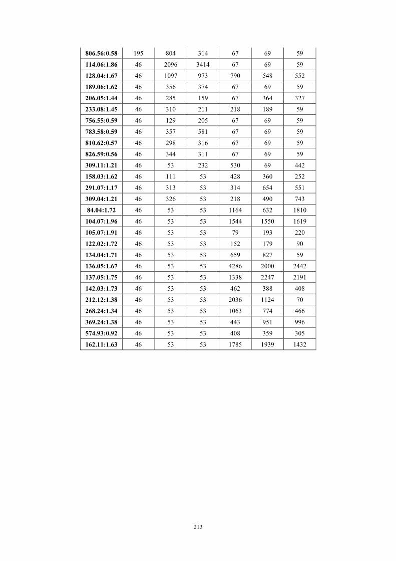
213

806.56:0.58 195 804 314 67 69 59

114.06:1.86 46 2096 3414 67 69 59

128.04:1.67 46 1097 973 790 548 552

189.06:1.62 46 356 374 67 69 59

206.05:1.44 46 285 159 67 364 327

233.08:1.45 46 310 211 218 189 59

756.55:0.59 46 129 205 67 69 59

783.58:0.59 46 357 581 67 69 59

810.62:0.57 46 298 316 67 69 59

826.59:0.56 46 344 311 67 69 59

309.11:1.21 46 53 232 530 69 442

158.03:1.62 46 111 53 428 360 252

291.07:1.17 46 313 53 314 654 551

309.04:1.21 46 326 53 218 490 743

84.04:1.72 46 53 53 1164 632 1810

104.07:1.96 46 53 53 1544 1550 1619

105.07:1.91 46 53 53 79 193 220

122.02:1.72 46 53 53 152 179 90

134.04:1.71 46 53 53 659 827 59

136.05:1.67 46 53 53 4286 2000 2442

137.05:1.75 46 53 53 1338 2247 2191

142.03:1.73 46 53 53 462 388 408

212.12:1.38 46 53 53 2036 1124 70

268.24:1.34 46 53 53 1063 774 466

369.24:1.38 46 53 53 443 951 996

574.93:0.92 46 53 53 408 359 305

162.11:1.63 46 53 53 1785 1939 1432

214

Table A3: Top 20 metabolite features with significant P-values.

Metabolite Feature logFC AveExpr t P. Value

adj. P. Value

104.07:1.96 1520.4516 810.8925 27.654404 1.16E-06 0.000170932 162.11:1.63 1667.9802 884.6568 11.614453 8.33E-05 0.005760181 176.05:1.61 1559.64 1480.4657 10.815728 1.18E-04 0.005760181 137.05:1.75 1874.8311 988.0822 6.999526 9.19E-04 0.025983784 130.05:1.72 838.9134 2476.0347 6.970562 9.36E-04 0.025983784 142.03:1.73 368.5252 234.9293 6.783939 1.06E-03 0.025983784 127.06:1.84 -412.7134 271.3567 -5.937015 1.94E-03 0.040705022 574.93:0.92 306.7802 204.0567 5.363985 3.03E-03 0.053414035 731.61:0.58 -302.4004 216.2002 -5.163905 3.58E-03 0.053414035 147.07:1.72 3084.9897 7005.6386 5.142872 3.64E-03 0.053414035 313.28:1.00 -523.4178 326.7089 -5.032628 4.00E-03 0.053414035 136.05:1.67 2858.654 1479.9937 4.549604 6.12E-03 0.064337289 369.24:1.38 746.2683 423.8008 4.481284 6.52E-03 0.064337289 162.08:1.64 987.0945 2570.0676 4.43253 6.82E-03 0.064337289 268.24:1.34 716.9438 409.1386 4.411864 6.95E-03 0.064337289 90.08:2.08 -2114.1302 3648.0152 -4.404063 7.00E-03 0.064337289 760.60:0.59 -1561.5327 1652.2808 -4.107784 9.29E-03 0.080355881 158.03:1.62 276.5577 208.3144 3.909564 1.13E-02 0.092365201 84.04:1.72 1151.1519 626.2426 3.724861 1.37E-02 0.105643351 761.60:0.59 -662.953 786.1506 -3.532025 1.67E-02 0.122865437

215

R Code

#Data input and adjusted-t test dat <- read.csv("/Users/Nancy/Dropbox/A-STAT/xing.csv",header = TRUE, row.names = 1) targ <- read.csv("/Users/Nancy/Dropbox/A-STAT/targxing.csv") head(targ) f <- factor(targ$target, levels=c("O","E")) design <- model.matrix(~0+f) colnames(design) <- c("O","E") contrastNames=c("O-E") contrastMatrix=matrix(c( -1,1),nrow=ncol(design)) colnames(contrastMatrix)=contrastNames contrastMatrix library(limma) fit=lmFit(dat,design=design) fit2=contrasts.fit(fit,contrasts=contrastMatrix) names(fit2) fit2=eBayes(fit2) F.stat=fit2$F p.value=fit2$F.p.value results=classifyTestsF(fit2,p.value=1.0E-1) write.csv(fit2,file="/Users/Nancy/Dropbox/A-STAT/xingresults.csv") topTable(fit2,n=20,coef="O-E") #Cluster analysis (Hierarchical) biomarker<-read.csv("/Users/Nancy/Dropbox/A-STAT/biomarker.csv",header = TRUE, row.names = 1)

d<-dist(biomarker, method ="euclidean") fit<-hclust(d) plot(fit)

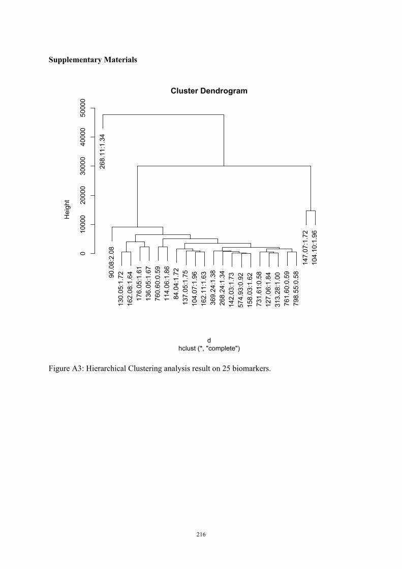
216

Supplementary Materials

Figure A3: Hierarchical Clustering analysis result on 25 biomarkers.

268.11:1.34

90.08:2.08

130.05:1.72

162.08:1.64

176.05:1.61

136.05:1.67

760.60:0.59

114.06:1.86

84.04:1.72

137.05:1.75

104.07:1.96

162.11:1.63

369.24:1.38

268.24:1.34

142.03:1.73

574.93:0.92

158.03:1.62

731.61:0.58

127.06:1.84

313.28:1.00

761.60:0.59

798.55:0.58147.07:1.72

104.10:1.96

010000

20000

30000

40000

50000

Cluster Dendrogram

hclust (*, "complete")d

Height

217

Appendix B

Cleaning Procedure for Resistive Glass Ion Mobility Mass

Spectrometer

1. Turn off the heater, let instrument completely cool down.

2. Turn off the turbo pump.

3. After 30 minutes to 1 hour, turn off the side pump aside the instrument by

double turning the red handle.

4. After another 30 minutes, turn off the rough pump at the back of the instrument

by disconnecting the power.

5. Start dissembling the IMS from the MS.

a. Take off ESI.

b. Take out the gate and store it in aluminum foil.

c. Take off the heat jacket.

d. Unscrew all the screws that connect the IMS and MS.

e. Undo all the leads connection and remove the grey box.

f. Flip the IMS straight up. (Only move with the base. No twist on the resistive

glass tube)

218

Front view of Quadruple 1 as part of the interface:

Cover it with aluminum foil:

Clean dusts on the bottom

219

Dissemble the resistive glass IMS piece by piece:

Ceramic piece between dissolvation tube and drift tube is cracked seriously:

Dirty inside the

tube

220

The IMS end, nozzle and lens:

In order to separate the parts from the metal frame, slightly push the metal showerhead. After

separating the parts, undo the leads and unscrew the metal leads.

Front view of IMS end, nozzle and lens:

Back view of IMS end, nozzle and lens:

221

Unscrew the metal leads and take apart the IMS end, nozzle and lens separately:

Please note that the white piece is an insulator between nozzle and lens.

222

Here are all the parts:

223

6. Cleaning procedure.

a. Rinse the parts with DI water.

b. Use soap solution to clean the resistive glass tubes througoutly.

c. Rinse the resistive glass tubes by DI water for about 10 minutes.

d. Soak the resistive glass tubes using a series of cleaning solvents including

methanol, methylene chloride, acetone and methanol.

224

Put the metal pieces and ceramic pieces into a large beaker and sonicate them in a series of

solutions including water, methanol, methylene chloride, acetone and methanol.

7. Reassembling.

a. Put together the IMS end, nozzle and lens.

b. Assemble IMS end, nozzle and lens into the metal frame.

c. Put the resistive glass tubes and IMS gate back on piece by piece.

d. Couple the IMS with the MS.

225

Put together the IMS end, nozzle and lens.

Matching up the two ceramic pieces by lining up the 2 holes on top.

226

Complete assembling IMS end, nozzle and lens by putting 4 springs in place.

Put the flat showerhead metal piece on top of the springs while match the gas holes.

227

Put the resistive glass tubes and ion gate piece by piece.

230

Make sure all the springs, nuts and screws are in the right place.

Then flip the IMS to its original position. Clean and put the O ring back on the interface for vacuum seal

231

Tight the screws against the rest of the interface.

Slide in the gate to make sure ceramic piece is in the right place.

8. Put on heating case.

9. Turn on the rough pump behind the instrument.

10. After 30 minutes, turn on the side pump and switch on the red handle.

11. After 20 minutes, turn on the turbo pump and wait till the pressure stabilized.

application of hadamard transform ion mobility mass

Documents

Transcript of application of hadamard transform ion mobility mass