Statistical Convergence and Convergence in Statistics

Statistical Convergence and Convergence in Statistics

Mark Burgina, Oktay Dumanb

aDepartment of Mathematics, University of California, Los Angeles, California 90095-1555, USA

bTOBB Economics and Technology University, Faculty of Arts and Sciences, Department of Mathematics,

Sögütözü 06530, Ankara, Turkey

Abstract

Statistical convergence was introduced in connection with problems of series

summation. The main idea of the statistical convergence of a sequence l is that the majority of elements from l converge and we do not care what is going on with other elements. We show (Section 2) that being mathematically formalized the concept of statistical convergence is directly connected to convergence of such statistical characteristics as the mean and standard deviation. At the same time, it known that sequences that come from real life sources, such as measurement and computation, do not allow, in a general case, to test whether they converge or statistically converge in the strict mathematical sense. To overcome limitations induced by vagueness and uncertainty of real life data, neoclassical analysis has been developed. It extends the scope and results of the classical mathematical analysis by applying fuzzy logic to conventional mathematical objects, such as functions, sequences, and series. The goal of this work is the further development of neoclassical analysis. This allows us to reflect and model vagueness and uncertainty of our knowledge, which results from imprecision of measurement and inaccuracy of computation. In the context on the theory of fuzzy limits, we develop the structure of statistical fuzzy convergence and study its properties. Relations between statistical fuzzy convergence and fuzzy convergence are considered in Theorems 3.1 and 3.2. Algebraic structures of statistical fuzzy limits are described in Theorem 3.5. Topological structures of statistical fuzzy limits are described in Theorems 3.3 and 3.4. Relations between statistical fuzzy convergence and fuzzy convergence of statistical characteristics, such as the mean (average) and standard deviation, are studied in Section 4. Introduced constructions and obtained results open new directions for further research that are considered in the Conclusion.

Keywords: statistical convergence, mean, standard deviation, fuzzy limit, statistics, fuzzy

convergence

Mark Burgin and Oktay Duman 2

1. Introduction

The idea of statistical convergence goes back to the first edition (published in Warsaw

in 1935) of the monograph of Zygmund [37]. Formally the concept of statistical

convergence was introduced by Steinhaus [34] and Fast [18] and later reintroduced by

Schoenberg [33].

Statistical convergence, while introduced over nearly fifty years ago, has only

recently become an area of active research. Different mathematicians studied properties

of statistical convergence and applied this concept in various areas such as measure

theory [30], trigonometric series [37], approximation theory [16], locally convex spaces

[29], finitely additive set functions [14], in the study of subsets of the Stone-Chech

compactification of the set of natural numbers [13], and Banach spaces [15].

However, in a general case, neither limits nor statistical limits can be calculated or

measured with absolute precision. To reflect this imprecision and to model it by

mathematical structures, several approaches in mathematics have been developed: fuzzy

set theory, fuzzy logic, interval analysis, set valued analysis, etc. One of these approaches

is the neoclassical analysis (cf., for example, [7, 8]). In it, ordinary structures of analysis,

that is, functions, sequences, series, and operators, are studied by means of fuzzy

concepts: fuzzy limits, fuzzy continuity, and fuzzy derivatives. For example, continuous

functions, which are studied in the classical analysis, become a part of the set of the fuzzy

continuous functions studied in neoclassical analysis. Neoclassical analysis extends

methods of classical calculus to reflect uncertainties that arise in computations and

measurements.

The aim of the present paper is to extend and study the concept of statistical

convergence utilizing a fuzzy logic approach and principles of the neoclassical analysis,

which is a new branch of fuzzy mathematics and extends possibilities provided by the

classical analysis [7, 8]. Ideas of fuzzy logic have been used not only in many

applications, such as, in bifurcation of non- linear dynamical systems, in the control of

chaos, in the computer programming, in the quantum physics, but also in various

Statistical Convergence and Convergence in Statistics 3

branches of mathematics, such as, theory of metric and topological spaces, studies of

convergence of sequences and functions, in the theory of linear systems, etc.

In the second section of this paper, going after introduction, we remind basic

constructions from the theory of statistical convergence consider relations between

statistical convergence, ergodic systems, and convergence of statistical characteristics

such as the mean (average), and standard deviation. In the third section, we introduce a

new type of fuzzy convergence, the concept of statistical fuzzy convergence, and give a

useful characterization of this type of convergence. In the fourth section, we consider

relations between statistical fuzzy convergence and fuzzy convergence of statistical

characteris tics such as the mean (average) and standard deviation.

For simplicity, we consider here only sequences of real numbers. However, in a

similar way, it is possible to define statistical fuzzy convergence for sequences of

complex numbers and obtain similar properties.

2. Convergence in statistics

Statistics is concerned with the collection and analysis of data and with making

estimations and predictions from the data. Typically two branches of statistics are

discerned: descriptive and inferential. Inferential statistics is usually used for two tasks: to

estimate properties of a population given sample characteristics and to predict properties

of a system given its past and current properties. To do this, specific statistical

constructions were invented. The most popular and useful of them are the average or

mean (or more exactly, arithmetic mean) µ and standard deviation σ (variance σ2).

To make predictions for future, statistics accumulates data for some period of time. To

know about the whole population, samples are used. Normally such inferences (for future

or for population) are based on some assumptions on limit processes and their

convergence. Iterative processes are used widely in statistics. For instance the empirical

approach to probability is based on the law (or better to say, conjecture) of big numbers,


states that a procedure repeated again and again, the relative frequency probability tends

to approach the actual probability. The foundation for estimating population parameters

and hypothesis testing is formed by the central limit theorem, which tells us how sample

means change when the sample size grows. In experiments, scientists measure how

statistical characteristics (e.g., means or standard deviations) converge (cf., for example,

[23, 31]).

Convergence of means/averages and standard deviations have been studied by many

authors and applied to different problems (cf. [1-4, 17, 19, 20, 24-28, 35]). Convergence

of statistical characteristics such as the average/mean and standard deviation are rela ted

to statistical convergence as we show in this section and Section 4.

Consider a subset K of the set N of all natural numbers. Then Kn = {k ∈ K; k ≤ n}.

Definition 2.1. The asymptotic density d(K) of the set K is equal to

limn→∞ (1/n) |Kn|

whenever the limit exists; here |B | denotes the cardinality of the set B.

Let us consider a sequence l = {ai ; i = 1,2,3,…} of real numbers, real number a, and

the set Lε (a) = {i ∈ N; |ai - a | ≥ ε }.

Definition 2.2. The asymptotic density, or simply, density d(l) of the sequence l with

respect to a and ε is equal to d(Lε (a)).

Asymptotic density allows us to define statistical convergence.

Definition 2.3. A sequence l = {ai ; i = 1, 2, 3, …} is statistically convergent to a if

d(Lε (a)) = 0 for every ε > 0. The number (point a) is called the statistical limit of l. We

denote this by a = stat-lim l.


Note that convergent sequences are statistically convergent since all finite subsets of

the natural numbers have density zero. However, its converse is not true [21, 33]. This is

also demonstrated by the following example.

Example 2.1. Let us consider the sequence l = {ai ; i = 1,2,3,…} whose terms are

i when i = n2 for all n = 1,2,3,…

ai =

1/i otherwise.

Then, it is easy to see that the sequence l is divergent in the ordinary sense, while 0 is

the statistical limit of l since d(K) = 0 where K = {n2 for all n = 1,2,3,…}.

Not all properties of convergent sequences are true for statistical convergence. For

instance, it is known that a subsequence of a convergent sequence is convergent.

However, for statistical convergence this is not true. Indeed, the sequence h = {i ; i =

1,2,3,…} is a subsequence of the statistically convergent sequence l from Example 2.1.

At the same time, h is statistically divergent.

However, if we consider dense subsequences of fuzzy convergent sequences, it is

possible to prove the corresponding result.

Definition 2.4. A subset K of the set N is called statistically dense if d(K) = 1.

Example 2.2. The set { i ≠ n2 ; i = 1,2,3,…; n = 1,2,3,…} is statistically dense, while

the set { 3i; i = 1,2,3,…} is not.

Lemma 2.1. a) A statistically dense subset of a statistically dense set is a statistically

dense set.

b) The intersection and union of two statistically dense sets are statistically dense sets.

Definition 2.5. A subsequence h of the sequence l is called statistically dense in l if

the set of all indices of elements from h is statistically dense.


Corollary 2.1. a) A statistically dense subsequence of a statistically dense

subsequence of l is a statistically dense subsequence of l.

b) The intersection and union of two statistically dense subsequences are statistically

dense subsequences.

Theorem 2.1. A sequence l is statistically convergent if and only if any statistically

dense subsequence of l is statistically convergent.

Proof. Necessity. Let us take a statistically convergent sequence l = {ai ; i = 1,2,3,…}

and a statistically dense subsequence h = {bk ; k =1,2,3,…} of l. Let us also assume that h

statistically diverges. Then for any real number a, there is some ε > 0 such that

liminfn? 8 (1/n) |Hn,ε(a)| = d > 0 for some d ∈ (0, 1), where Hn,ε(a) = {k ≤ n; |bk – a| > ε}.

As h is a subsequence of l, we have Ln,ε(a) ⊇ Hn,ε(a) where Ln,ε(a) = {i ≤ n; | ai – a| > ε}.

Consequently, liminfn? 8 (1/n)|Ln,ε(a)| ≥ d > 0, which yields that d({i; | ai – a| > ε}) ≠ 0.

Thus, l is also statistically divergent.

Sufficiency follows from the fact that l is a statistically dense subsequence of itself.

Corollary 2.1. A statistically dense subsequence of a statistically convergent

sequence is statistically convergent.

To each sequence l = {ai ; i = 1,2,3,…} of real numbers, it is possible to correspond a

new sequence µ(l) = {µn = (1/n) Σi=1n ai ; n = 1,2,3,…} of its partial averages (means).

Here a partial average of l is equal to µn = (1/n) Σi=1n ai .

Sequences of partial averages/means play an important role in the theory of ergodic

systems [5]. Indeed, the definition of an ergodic system is based on the concept of the

“time average” of the values of some appropriate function g arguments for which are

dynamic transformations T of a point x from the manifold of the dynamical system. This

average is given by the formula

g(x) = lim (1/n) Σk=1n-1 g(Tkx).


In other words, the dynamic average is the limit of the partial averages/means of the

sequence { Tkx ; k =1,2,3,…}.

Let l = {ai ; i = 1,2,3,…} be a bounded sequence, i.e., there is a number m such that

|ai| < m for all i∈N. This condition is usually true for all sequences generated by

measurements or computations, i.e., for all sequences of data that come from real life.

Theorem 2.2. If a = stat-lim l, then a = lim µ(l).

Proof. Since a = stat-lim l, for every ε > 0, we have

(2.1) limn→∞ (1/n) |{i ≤ n, i ∈ N; |ai - a| ≥ ε}| = 0.

As |ai| < m for all i∈ N, there is a number k such that |ai - a| < k for all i∈ N. Namely, | ai -

a| ≤ | ai | + | a| ≤ m + | a| = k. Taking the set Ln,ε (a) = {i ≤ n, i ∈ N; | ai - a| ≥ ε}, denoting

|Ln,ε (a)| by un , and using the hypothesis |ai| < m for all i∈ N, we have the following

system of inequalities:

|µn -a| = |(1/n) Σi=1n ai - a|

≤ (1/n) Σi=1n | ai - a|

≤ (1/n) {kun + ( n - un)ε}

≤ (1/n) (kun + nε )

= ε + k (un/n).

From the equality (2.1), we get, for sufficiently large n, the inequality |µn -a| < ε +k ε.

Thus, a = lim µ(l).

Theorem is proved.

Remark 2.1. However, convergence of the partial averages/means of a sequence does

not imply statistical convergence of this sequence as the following example demonstrates.


ai = (-1)i √ i . This sequence is statistically divergent although lim µ(l) = 0.


Taking a sequence l = {ai ; i = 1,2,3,…} of real numbers, it is possible to construct not

only the sequence µ(l) = { µn = (1/n) Σi=1n ai ; n = 1,2,3,…} of its partial averages

(means) but also the sequences σ(l) = {σn = ((1/n) Σi=1n (ai - µn) 2)½ ; n = 1,2,3,…} of its

partial standard deviations σn and σ2(l) = {σn2 = (1/n) Σi=1

n (ai - µn) 2 ; n = 1,2,3,…} of its

partial variances σn2.

Theorem 2.3. If a = stat-lim l and | ai | < m for all i∈ N, then lim σ(l) = 0.

Proof. We will show that lim σ2(l) = 0. By the definition, σn2 = (1/n) Σi=1

n (ai - µn)2 =

(1/n) Σi=1n (ai)2 - µn

2. Thus, lim σ2(l) = limn→∞ (1/n) Σi=1n (ai)2 - limn→∞ µn

2.

If | ai| < m for all i∈ N, then there is a number p such that | ai2

- a2| < p for all i∈ N.

Namely, | ai 2 - a2| ≤ | ai |2 + | a|2 < m2 + | a|2 < m2 + | a|2 + m + | a| = p. Let us consider the

absolute value of the difference µn 2 - (1/n) Σi=1

n (ai)2 = σ2n . Taking the set Ln,ε (a) = {i ≤

n, i ∈ N; | ai - a| ≥ ε }, denoting |Ln,ε (a)| by un, and using the hypothesis |ai | < m for all i∈

N, we have the following system of inequalities:

|σ2n | = | (1/n) Σi=1

n (ai)2 - µn

2 |

= | (1/n) Σi=1n (ai

2 - a2) - (µn2 – a2)|

≤ (1/n) Σi=1n | ai

2 - a2| + |µn2 – a2|

< (p/n) Σi=1n |ai - a| + |µn

2 – a2|

< (p/n) (un + (n - un)ε) + |µn2 – a2|

< (p/n) (un + nε) + |µn2 – a2|

= p (un /n) + εp + |µn2 – a2|

as |ai2 - a2| ≤ |ai - a| |ai + a| < |ai - a| ⋅ p. By Theorem 2.2, we have a = lim µ(l), which

guarantees that lim µn2 = a2. Also by (2.1) lim (un /n) = 0. Since ε > 0 was arbitrary, the


right hand side of the above inequality tends to zero as n → ∞. Therefore, we have

lim σ(l) = 0.

Theorem is proved.

Corollary 2.2. If a = stat-lim l and | ai | < m for all i∈ N, then lim σ2(l) = 0.

Theorem 2.4. A sequence l is statistically convergent if its sequence of partial

averages µ(l) converges and ai ≤ lim µ(l) (or ai ≥ lim µ(l)) for all i = 1, 2, 3, … .

Proof. Let us assume that a = lim µ(l), ai ≤ lim µ(l) and take some ε > 0, the set Ln,ε(a)

= {i ≤ n, i ∈ N; |ai - a| ≥ ε}, and denote |Ln,ε (a)| by un . Then we have

| a - µn | = | a - (1/n) Σi=1n ai |

= |(1/n) Σi=1n (a - ai)|

= (1/n) Σi=1n (a - ai)

≥ (1/n) Σ| ai - a | ≥ ε (a - ai)

≥ (un/n)ε

Consequently, limn→∞ | a - µn| ≥ limn→∞ (un/n) ε. As limn→∞ | a - µn| =0 and ε is a fixed

number, we have limn→∞ (1/n) |{i ≤ n, i ∈ N; | ai - a| ≥ ε }| = 0, i.e., a = stat-lim l.

The case when ai ≥ lim µ(l)) for all i = 1, 2, 3, … is considered in a similar way.

Theorem is proved as ε is an arbitrary positive number.

Let l = {ai ; i = 1,2,3,…} be a bounded sequence, i.e., there is a number m such that |ai|

< m for all i∈N.

Theorem 2.5. A sequence l is statistically convergent if and only if its sequence of

partial averages µ(l) converges and its sequence of partial standard deviations σ(l)

converges to 0.

Proof. Necessity follows from Theorems 2.2 and 2.3.


Sufficiency. Let us assume that a = lim µ(l), lim σ(l) = 0, and take some ε > 0. This

implies that for any λ > 0, there is a number n such that λ > | a - µn| . Then taking a

number n such that it implies the inequality ε > λ, we have

σn2 = (1/n) Σi=1

n (ai - µn) 2

≥ (1/n) Σ{(ai - µn) 2 ; |ai - a| ≥ ε}

= (1/n) Σ{((ai - a) + (a - µn)) 2 ; |ai - a| ≥ ε}

(2.2) > (1/n) Σ{((ai - a) ± λ) 2 ; |ai - a| ≥ ε}

= (1/n) Σ{((ai - a) 2 ± 2λ(ai - a) + λ2); |ai - a| ≥ ε}

(2.3) = (1/n) Σ{(ai - µn) 2; |ai - a| ≥ ε} ± 2λ (1/n) Σ{(ai - a); |ai - a| ≥ ε}+ λ2

as (ai - µn) = (ai - a) + (a - µn) and we take + λ or - λ in the expression (2.2) according to

the following rules:

1) if (ai - a) ≥ 0 and (a - µn) ≥ 0, then (ai - a) + (a - µn) ≥ (ai - a) > (ai - a) - λ, and we

take - λ;

2) if (ai - a) ≥ 0 and (a - µn) ≤ 0, then (ai - a) + (a - µn) ≥ (ai - a) - |a - µn| > (ai - a) - λ,

and we take - λ;

3) if (ai - a) ≤ 0 and (a - µn) ≥ 0, then |(ai - a) + (a - µn)| = |(a - ai) - (a - µn)| >

|(a - ai) -λ| = |(ai - a) + λ|, and we take + λ;

4) if (ai - a) ≤ 0 and (a - µn) ≤ 0, then |(ai - a) + (a - µn)| ≥ | a - ai| > |(ai - a) + λ| as

ai - a < - ε, and we take + λ.

In the expression (2.3), it is possible to take a sequence {λk ; k = 1, 2, 3,…} such that

the sequence λk2 converges to 0 because the sequence {µn ; n = 1,2,3,…} converges to a

when n tends to ∞. The sum 2λk (1/n) Σ{(ai - a); |ai - a| ≥ ε} also converges to 0 when k

tends to ∞ because λk converges to 0 and (1/n) Σ (ai - a) < (1/n) Σ (|ai| + |a|) ≤ m + |a| .

At the same time, the sequence {σn; n = 1, 2, 3,…} also converges to 0. Thus, limn→∞


(1/n) Σ{(ai - µn) 2; |ai - a| ≥ ε} = 0. This implies that limn→∞ (1/n)Σ{|ai - µn|2; |ai - a| ≥ ε} =

0. At the same time, limn→∞ (1/n) Σ{|ai - µn|2; |ai - a| ≥ ε} ≥ ε⋅(limn→∞ (1/n) |{i ≤ n, i ∈ N;

|ai - a| ≥ ε}|). As ε is a fixed number, we have limn→∞ (1/n) |{i ≤ n, i ∈ N; | ai - a| ≥ ε}| = 0

for any ε > 0 as ε is an arbitrary positive number, i.e., a = stat-lim l.

Theorem is proved.

3. Statistical fuzzy convergence

Here we extend statistical convergence to statistical fuzzy convergence, which, as we

have discussed, is more realistic for real life applications.

For convenience, throughout the paper, r denotes a non-negative real number and l =

{ai ; i = 1,2,3,…} represents a sequence of real numbers.

Let us consider the set Lr,ε (a) = {i ∈ N; |ai - a| ≥ r + ε} and a non-negative real

number r ≥ 0.

Definition 3.1. A sequence l is statistically r-converges to a number a if d(Lr,ε (a)) = 0

for every ε > 0. The number (point a) is called a statistical r- limit of l. We denote this by

a = stat-r-lim l.

Definition 3.1 implies the following results.

Lemma 3.1. a) a = stat-r-lim l ⇔ ∀ ε > 0, limn→∞ (1/n) |{i ∈ N; i ≤ n ; |ai - a| ≥ r +

ε}| = 0.

b) a = stat-r-lim l ⇔ ∀ ε > 0, limn→∞ (1/n) |{i ∈ N; i ≤ n ; |ai - a| < r + ε}| = 1.


Remark 3.1. We know from [8] that if a = lim l (in the ordinary sense), then for any r

≥ 0, we have a = r- lim l. In a similar way, using Definition 3.1, we easily see that if a = r-

lim l, then we have a = stat-r-lim l since every finite subset of the natural numbers has

density zero. However, its converse is not true as the following example of a sequence

that is statistically r-convergent but not r-convergent and also not statistically convergent.

shows.


i when i = n2 for all n = 1,2,3,…

(3.1) ai =

(-1)i otherwise.

Then, it is easy to see that the sequence l is divergent in the ordinary sense. Even more,

the sequence l has no r-limits for any r since it is unbounded from above (see Theorem

2.3 from [8]).

On the other hand, we see that the sequence x is not statistically convergent because it

does not satisfy the Cauchy condition for statistical convergence [21].

At the same time, 0 = stat-1-lim l since d(K) = 0 where K = {n2 for all n = 1,2,3,…}.

Lemma 3.2. Statistical 0-convergence coincides with the concept of statistical

convergence.

This result shows that statistical fuzzy convergence is a natural extension of statistical

convergence.

Lemma 3.3. If a = stat-lim l, then a = stat-r-lim l for any r ≥ 0.

Lemma 3.4. If a = stat-r- lim l, then a = stat-q-lim l for any q > r.


Lemma 3.5. If a = stat-r- lim l and |b – a | = p, then b = stat-q-lim l where q = p + r.

It is known that a subsequence of a fuzzy convergent sequence is fuzzy convergent

[8]. However, for statistical convergence this is not true. Indeed, the sequence h = {i ; i =

1,2,3,…} is a subsequence of the statistically fuzzy convergent sequence l from Example

3.1. At the same time, h is statistically fuzzy divergent.

However, if we consider dense subsequences of statistically fuzzy convergent

sequences, it is possible to prove the following result.

Theorem 3.1. A sequence is statistically r-convergent if and only if any its

statistically dense subsequence is statistically r-convergent.

Proof. Necessity. Let us take a statistically r-convergent sequence l = {ai ; i =

1,2,3,…} and a statistically dense subsequence h = {bk ; k = 1,2,3,…} of l. Let us also

assume that h statistically r-diverges. Then for any real number a, there is some ε > 0

such that d(Hε(a)) > 0 where Hε(a) = {k; |bk – a| > r + ε }. As h is a subsequence of l, we

have Lε(a) ⊇ Hε(a) where Lε(a) = {i; |ai – a| > r + ε}. Consequently, d(Hε(a)) > 0 as the

subsequence h is statistically dense in l. Thus, l is also statistically r-divergent.

Sufficiency follows from the fact that l is a statistically dense subsequence of itself.

Theorem is proved.

A statistically r-convergent sequence contains not only dense statistically r-

convergent subsequences, but also dense r-convergent subsequences.

Theorem 3.2. a = stat-r-lim l if and only if there exists an increasing index sequence

K = {kn ; kn ∈ N, n = 1,2,3,…} of the natural numbers such that d(K) = 1 and a = r- lim lK

where lK = {ai ; i ∈ K}.

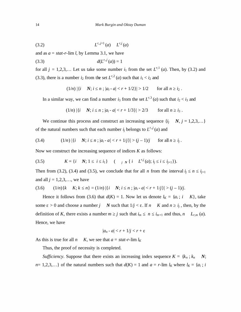
Proof. Necessity. Suppose that a = stat-r-lim l. Let us consider sets Lr,,j (a) = {i ∈ N;

|ai - a| < r + (1/j) } for all j = 1,2,3,… By the definition, we have


(3.2) Lr,,j+1 (a) ⊆ Lr,j (a)

and as a = stat-r-lim l, by Lemma 3.1, we have

(3.3) d(Lr,,j (a)) = 1

for all j = 1,2,3,… Let us take some number i1 from the set Lr,1 (a). Then, by (3.2) and

(3.3), there is a number i2 from the set Lr,2 (a) such that i1 < i2 and

(1/n) |{i ∈ N; i ≤ n ; |ai - a| < r + 1/2}| > 1/2 for all n ≥ i2 .

In a similar way, we can find a number i3 from the set Lr,3 (a) such that i2 < i3 and

(1/n) |{i ∈ N; i ≤ n ; |ai - a| < r + 1/3}| > 2/3 for all n ≥ i3 .

We continue this process and construct an increasing sequence {ij ∈ N, j = 1,2,3,…}

of the natural numbers such that each number ij belongs to Lr,,j (a) and

(3.4) (1/n) |{i ∈ N; i ≤ n ; |ai - a | < r + 1/j}| > (j – 1)/j for all n ≥ ij .

Now we construct the increasing sequence of indices K as follows:

(3.5) K = {i ∈ N; 1 ≤ i ≤ i1} ∪ (∪ j∈N { i ∈ Lr,j (a); ij ≤ i ≤ ij+1}).

Then from (3.2), (3.4) and (3.5), we conclude that for all n from the interval ij ≤ n ≤ ij+1

and all j = 1,2,3,…, we have

(3.6) (1/n){k ∈ K; k ≤ n} = (1/n) |{i ∈ N; i ≤ n ; |ai - a| < r + 1/j}| > (j – 1)/j.

Hence it follows from (3.6) that d(K) = 1. Now let us denote lK = {ai ; i ∈ K}, take

some ε > 0 and choose a number j ∈ N such that 1/j < ε. If n ∈ K and n ≥ ij , then, by the

definition of K, there exists a number m ≥ j such that im ≤ n ≤ im+1 and thus, n ∈ Lr,m (a).

Hence, we have

|an - a| < r + 1/j < r + ε

As this is true for all n ∈ K, we see that a = stat-r-lim lK

Thus, the proof of necessity is completed.

Sufficiency. Suppose that there exists an increasing index sequence K = {kn ; kn ∈ N;

n= 1,2,3,…} of the natural numbers such that d(K) = 1 and a = r-lim lK where lK = {ai ; i


∈ K}. Then there is a number n such that for each i from K such that i ≥ n, the inequality

|ai - a| < r + ε holds. Let us consider the set

Lr,ε (a) = {i ∈ N; |ai - a| ≥ r + ε}

Then we have

Lr,ε (a) ⊆ N \ {ki ; ki ∈ N; i = n, n +1, n + 2,…}

Since d(K) = 1, we get d(N \ {ki ; ki ∈ N; i = n, n +1, n + 2,…}) = 0, which yields

d(Lr,ε(a)) = 0 for every ε > 0. Therefore, we conclude that a = stat-r-lim l.

Theorem is proved.

Corollary 3.1 [32]. a = stat-lim l if and only if there exists an increasing index

sequence K = {kn ; kn ∈ N; n = 1,2,3,…} of the natural numbers such that d(K) = 1 and a

= lim lK where lK = {ai ; i ∈ K}.

Corollary 3.2. a = stat-r-lim l if and only if there exists a sequence h = {bi ; i =

1,2,3,…} such that d({i; ai = bi }) = 1 and a = r-lim h.

Corollary 3.3. The following statements are equivalent:

(i) a = stat-r- lim l.

(ii) There is a set K ⊆ N such that d(K) = 1 and a = r- lim lK where lK = {ai ; i ∈ K}.

(iii) For every ε > 0, there exist a subset K ⊆ N and a number m ∈ K such that d(K) =

1 and |an - a| < r + ε for all n ∈ K and n ≥ m.

We denote the set of all statistical r- limits of a sequence l by Lr-stat (l), that is,

Lr-stat (l) = {a ∈ R; a = stat-r-lim l}.

Then we have the following result.

Theorem 3.3. For any sequence l and number r ≥ 0, Lr-stat (l) is a convex subset of the

real numbers.


Proof. Let c, d ∈ Lr-stat (l), c < d and a ∈ [c, d]. Then it is enough to prove that a ∈ Lr-stat (l).

Since a ∈ [c, d], there is a number λ ∈ [0, 1] such that. a = λc - (1-λ)d. As c, d ∈ Lr-stat (l), then

for every ε > 0, there exist index sets K1 and K2 with d(K1) = d(K2) = 1 and the numbers n1 and

n2 such that |ai - c| < r + ε for all i from K1 and i ≥ n1 and |ai - d| < r + ε for all i from K2 and i ≥

n2 . Let us put K = K1 ∩ K2 and n = max{n1, n2}. Then d(K) = 1 and for all i ≥ n1 with i from K,

we have

| ai - a | = | ai - λc - (1-λ)d|

= |(λai - λc) + ((1-λ) ai - (1-λ)d)|

≤ |λai - λc| + |(1-λ) ai - (1-λ)d |

≤ λ(r + ε) + (1-λ)(r + ε) = r + ε.

So, by Theorem 3.1, we conclude a = stat-r- lim l, which implies a ∈ Lr-stat (l).

Theorem is proved.

Lemmas 3.4 and 3.5 imply the following result.

Proposition 3.1. If q > r, then Lr-stat (l) ⊂ Lq-stat (l).

Definition 3.2. The quantity

inf{r ; a = stat-r- lim l}

is called the upper statistical defect δ(a = stat-lim l) of statistical convergence of l to the

number a.

Proposition 3.2. If q = inf {r; a = stat-r- lim l}, then a = stat-q-lim l.

Definition 3.3. The quantity

1

1 + δ(a = stat-lim l)


is called the upper statistical measure µ(a = stat-lim l) of statistical convergence of l to a

number a.

The upper statistical measure of statistical convergence of l defines the fuzzy set Lstat

(l) = [R, µ(a = stat-lim l)], which is called the complete statistical fuzzy limit of the

sequence l.

Example 3.2. We find the complete statistical fuzzy limit Lstat (l) of the sequence l

from Example 3.1. For this sequence and a real number a, we have

µ(a = stat-lim l) = 1/(2 + |a|)

This fuzzy set Lstat (l) is presented in Figure 1.

Figure 1. The complete statistical fuzzy limit of the sequence l from Example 3.1.

a

µ(a =stat-lim l )


Definition 3.4 [36]. A fuzzy set [A, µ] is called convex if its membership function

µ(x) satisfies the following condition: µ(?x + (1 - ?)z) = min{µ(x), µ(z)} for any x, z and

any number ? > 0.

Then we have the following result.

Theorem 3.4. The complete statistical fuzzy limit Lstat (l) = {a, µ(a = stat-r-lim l); a

∈ R} of a sequence l is a convex fuzzy set.

Proof. Let c, d ∈ Lr-stat (l), c < d and a ∈ [c, d]. Then it is enough to prove that µ(a =

stat-lim l) = µ( (?c + (1 - ?)d) = stat-lim l) = min{µ(c = stat-lim l), µ(d = stat-lim l )}. This

is equivalent to the inequality δ(a = stat-lim l) = δ( (?c + (1 - ?)d) = stat-lim l) ≤ max{δ(c =

stat-lim l), δ(d = stat-lim l )}.

Let us assume, for convenience, that q =δ(c = stat-lim l) = r = δ(d = stat-lim l )}. Then

by Lemma 3.4, d = stat-q-lim l. Then by Theorem 3.3, d = stat-q-lim l as the set Lr-stat (l) is

convex. Thus, δ(a = stat-lim l) ≤ q = max{δ(c = stat-lim l), δ(d = stat-lim l )}.

Theorem is proved.

Definition 3.5 [36]. A fuzzy set [A, µ] is called normal if sup µ(x) = 1.

Theorem 3.4 allows us to prove the following result.

Theorem 3.5. The complete statistical fuzzy limit Lstat (l) = {a, µ(a = stat-r-lim l); a ∈

R} of a sequence l is a normal fuzzy set if and only if l statistically converges.

Let l = {ai∈R; i = 1,2,3, …}and h = {bi∈R; i = 1,2,3, …}. Then their sum l + h is

equal to the sequence {ai + bi; i = 1,2,3, …} and their difference l - h is equal to the

sequence {ai - bi; i = 1,2,3, …}. Lemma 2.1 allows us to prove the following result.

Theorem 3.6. If a = stat-r-lim l and b = stat-q-lim h, then:


(a) a + b = stat-(r+q)-lim(l+h) ;

(b) a - b = stat-(r+q)-lim(l - h) ;

(c) ka = stat-( |k|⋅r)- lim (kl) for any k∈R where kl = {kai ; i = 1,2,3,…}.

Corollary 3.3 [32]. If b = stat-lim l and c = stat-lim h, then:

(a) a + b = stat-lim (l+h) ;

(b) a - b = stat-lim (l - h) ;

(c) ka = stat-lim (kl) for any k∈R.

An important property in calculus is the Cauchy criterion of convergence, while an

important property in neoclassical analysis is the extended Cauchy criterion of fuzzy

convergence. Here we find an extended statistical Cauchy criterion for statistical fuzzy

convergence.

Definition 3.6. A sequence l is called statistically r-fundamental if for any ε > 0

there is n ∈ N such that d(Ln,r,ε) = 0 where Ln,r,ε = {i ∈ N; i ≤ n and |ai – an| ≥ r + ε}.

Definition 3.7. A sequence l is called statistically fuzzy fundamental if it is

statistically r- fundamental for some r ≥ 0.

Lemma 3.6. If r ≤ p, then any statistically r- fundamental sequence is statistically p-

fundamental.

Lemma 3.7. A sequence l is a statistically Cauchy sequence if and only if it is

statistically 0-fundamental.

This result shows that the property to be a statistically fuzzy fundamental sequenc e is

a natural extension of the property to be a statistically Cauchy sequence.


Using the similar technique as in proof of Theorem 3.2, one can obtain the following

result.

Theorem 3.7. A sequence l is statistically r-fundamental if and only if there exists an

increasing index sequence K = {kn ; kn ∈ N; n = 1,2,3,…} of the natural numbers such

that d(K) = 1 and the subsequence lK is r-fundamental, that is, for every ε > 0 there is a

number i such that |akn – aki | < r + ε for all n ≥ i.

Corollary 3.4. A sequence l is statistically fuzzy fundamental if and only if there

exists a statistically dense subsequence u such that u is fuzzy fundamental.

Theorem 3.6 yields the following result.

Corollary 3.5 [21]. A sequence l is a statistically Cauchy sequence if and only if

there exists an increasing index sequence K = {kn ; kn ∈ N; n = 1,2,3,…} of the natural

numbers such that d(K) = 1 and the subsequence lK is a Cauchy sequence.

Theorem 3.8 (The Extended Statistical Cauchy Criterion). A sequence l has a

statistical r-limit if and only if it is statistically r- fundamental.

Proof. Necessity. Let a = stat-r-lim l. Then by the definition, for any ε > 0, we have

d(Lr,ε (a)) = 0, in other words, limn→∞ (1/n) |{i ∈ N; i ≤ n ; |ai - a | ≥ r + ε/2}| = 0. This

implies that given ε > 0, we find n ∈ N such that for any i > n, we have |ai - an| ≤ |a - ai|

+ | a - an|. Consequently, d(Ln,r,ε) ≤ d(Lr,ε/2 (a)) + d(Lr,ε/2 (a)) = 0, i.e., d(Ln,r,ε) = 0 Thus, l

is a statistically r- fundamental sequence.

Sufficiency. Assume now that l is a statistically r-fundamental sequence. Then, by

Theorem 3.7, we conclude that there is an r-convergent u = {ui; i = 1,2,3,…} such that

d({i ; ai = ui}) = 1. We denote the r-limit of u is a. Now let A={i ∈ N; i ≤ n ; ai ≠ ui} and

B= {i ∈ N; i ≤ n ; |ui - a| ≥ r + ε}. Then observe that d(A) = d(B) = 0. On the other hand,

since for each n


Lr,ε (a) = {i ∈ N; i ≤ n; | ai - a | ≥ r + ε} ⊆ A ∪ B,

we have d(Lr,ε) = 0, which gives stat-r-lim l = a.

The proof is completed.

Theorem 3.8 directly implies the following results.

Corollary 3.6 (The General Fuzzy Convergence Criterion). The sequence l

statistically fuzzy converges if and only if it is statistically fuzzy fundamental.

Corollary 3.7 (The Statistical Cauchy Criterion) [21]. A sequence l statistically

converges if and only if it is statistically fundamental, i.e., for any ε > 0 there is n ∈ N

such that d(Ln,r,ε) = 0 where Ln,r,ε = {i ∈ N; | ai – an | ≥ ε}.

Corollary 3.8 (The Cauchy Criterion). The sequence l converges if and only if it is

fundamental.

4. Fuzzy convergence in statistics and statistical fuzzy convergence

In Section 2, we found relations between statistical convergence and convergence of

statistical characteristics (such as mean and standard deviation). However, when data are

obtained in experiments, they come from measurement and computation. As a result, we

never have and never will be able to have absolutely precise convergence of statistical

characteristics. It means that instead of ideal classical convergence, which exists only in

pure mathematics, we have to deal with fuzzy convergence, which is closer to real life

and gives more realistic models. That is why in this section, we consider relations

between statistical fuzzy convergence and fuzzy convergence of statistical characteristics.


Let l = {ai ; i = 1,2,3,…} be a bounded sequence, i.e., there is a number m such that

|ai| < m for all i∈ N. This condition is usually true for all sequences generated by

measurements or computations.

Theorem 4.1. If a = stat-r- lim l, then a = r- lim µ(l) where µ(l) = {µn = (1/n) Σi=1n ai;

n = 1, 2, 3, …}.

Proof. Since a = stat-r- lim l, for every ε > 0, we have

(4.1) limn→∞ (1/n) |{i ≤ n, i ∈ N; | ai - a| ≥ r + ε}| = 0.

If |ai| < m for all i∈ N, then there is a number k such that |ai - a| < k for all i∈ N. Namely,

|ai - a| ≤ |ai | + |a| ≤ m + |a| = k. Taking the set Ln,r,ε (a) = {i ∈ N; i ≤ n and | ai - a | ≥ r +

ε}, denoting |Ln,r,ε (a)| by un , and using the hypothesis |ai| < m for all i∈ N, we have the

following system of inequalities

|µn - a| = |(1/n) Σi=1n ai - a|

≤ (1/n) Σi=1n |ai - a|

≤ (1/n) (kun + (n - un)(r + ε))

≤ (1/n) (kun + n(r + ε))

= r + ε + (1/n) (kun).

From the equality (4.1), we get, for sufficiently large n, that the inequality |µn –a| ≤ r + 2ε

holds because the number k is fixed and the sequence {(1/n)un ; n = 1,2,3,…} converges

to zero. Thus, a = r- lim µ(l).

Theorem is proved.

Remark 4.1. Statistical r-convergence of a sequence does not imply r-convergence

of this sequence even if all elements are bounded as the following example demonstrates.


Example 4.1. Let us consider the sequence l = {ai ; i = 1,2,3,…} elements of which

are

(-1)i⋅1000 when i = n2 for all n = 1,2,3,…

ai =

(-1)i otherwise.

By the definition, 0 = stat-1-lim l since d(K) = 0 where K = {n2 for all n = 1,2,3,…}.

At the same time, this sequence does not have 1- limits.

Corollary 4.1. If sequence l is statistically fuzzy fundamental, then the sequence of

its partial means is fuzzy fundamental.

Finally, we get the following result.

Theorem 4.2. If a = stat-r-lim l and there is a number m such that |ai| < m for all i =

1,2,…, then 0 = [2pr]½-lim σ(l) where p = max {m2 + |a|2, m + |a|}.

Proof. We will first show that lim σ2(l) = 0. By the definition, σn2 = (1/n) Σi=1

n (ai -

µn)2 = (1/n) Σi=1n (ai)2 - µn

2. Thus, lim σ2(l) = limn→∞ (1/n) Σi=1n (ai)2 - limn→∞ µn

2. Since

|ai| < m for all i∈ N, there is a number p such that |ai2

- a2| < p for all i∈ N. Namely, | ai 2 -

a2| ≤ | ai|2 + |a|2 < m2 + |a|2 < max {m2 + | a|2, m + |a|} = p. Taking the set Ln,r,ε (a) = {i ∈

N; i ≤ n and | ai - a| ≥ r + ε}, denoting |Ln,r,ε (a)| by un , and using the hypothesis | ai| < m

for all i∈ N, we have the following system of inequalities:

|σ2n | = |(1/n) Σi=1

n (ai)2 - µn2 |

= |(1/n) Σi=1n (ai

2 - a2) - (µn2 – a2)|

≤ (1/n) Σi=1n | ai

2 - a2| + |µn2 – a2|

< (p/n) Σi=1n |ai - a| + |µn – a| |µn+a|

< (p/n) (un + (n - un)(r + ε)) + |µn– a| (|µn| + |a|)

≤ (p/n) (un + n (r + ε)) + |µn– a| ((1/n)Σi=1n |ai| + |a|)


< p (un /n) + p (r + ε) + p |µn– a|.

Now by hypothesis and Theorem 4.1, we have a = r-lim µ(l). Also, by (4.1), we have

lim (un /n) = 0. Then, for every ε > 0 and sufficiently large n, we have

(4.2) |σ2n | < p ε + p (r + ε) + p (r + ε) = 2pr + 3pε.

As (x + y)½ ≤ x½ + y½ for any x, y > 0, it follows from (4.2) that

|σn | ≤ [2pr]½ + (3pε)½,

which yields that 0 = [2pr]½- lim σ(l).

The proof is completed.

Fuzzy convergence of partial standard deviations implies corresponding fuzzy

convergence of partial variances.

Corollary 4.2. If a = stat-r- lim l and there is a number m such that | ai| < m for all i =

1, 2, 3, … , then 0 = [2pr]-lim σ2(l) where p = max {m2 + |a|2, m + |a|}.

5. Conclusion

We have developed the concept of statistical fuzzy convergence and studied its

properties. Relations between statistical fuzzy convergence and fuzzy convergence are

considered in Theorems 3.1 and 3.2. Algebraic structures of statistical fuzzy limits are

described in Theorem 3.5. Topological structures of statistical fuzzy limits are described

in Theorems 3.3 and 3.4. Relations between statistical convergence, ergodic systems, and

convergence of statistical characteristics, such as the mean (average), and standard

deviation, are studied in Sections 2 and 4. Introduced constructions and obtained results

open new directions for further research.

It would be interesting to develop connections between statistical fuzzy convergence

and fuzzy dynamical systems [9], introducing and studying ergodic systems.


It would also be interesting to study statistically fuzzy continuous functions, taking as

the base the theory of fuzzy continuous functions [7] and the theory of statistically

continuous functions [10].

The theory of regular summability method is an important topic in functional analysis

(see, for instance, [6, 22]). In recent years it has been demonstrated that statistical

convergence can be viewed as a regular method of series summability. In particular,

Connor showed [11] that statistical convergence is equivalent to the strong Cesaro

summability in the space of all series with bounded elements. Similar problems are

studied in [12]. Thus, it would also be interesting to study summability of series and

relations between statistical fuzzy convergence and summability methods.

References

[1] M. A. Akcoglu and L. Sucheston, Weak convergence of positive contractions implies strong convergence of averages, Probability Theory and Related Fields, 32 (1975) 139 – 145.

[2] M.A. Akcoglu and A. del Junco, Convergence of averages of point transformations, Proc. Amer. Math. Soc. 49 (1975) 265-266.

[3] I. Assani, Pointwise convergence of averages along cubes, preprint 2003, Math. DS/0305388, arxiv.org.

[4] I. Assani, Pointwise convergence of nonconventional averages, Colloq. Math. 102 (2005) 245- 262.

[5] P. Billingsley, Ergodic Theory and Information, John Wiley & Sons, New York, 1965.

[6] T.J. I’A Bromwich and T.M. MacRobert, An Introduction to the Theory of Infinite Series, 3rd ed. Chelsea, New York, 1991.

[7] M. Burgin, Neoclassical analysis: fuzzy continuity and convergence, Fuzzy Sets and Systems 75 (1995) 291-299.

[8] M.S. Burgin, Theory of fuzzy limits, Fuzzy Sets and Systems 115 (2000) 433-443.

[9] M. Burgin, Recurrent points of fuzzy dynamical systems, J. Dyn. Syst. Geom. Theor. 3 (2005) 1-14.


[10] J. Cervenansky, Statistical convergence and statistical continuity, Sbornik Vedeckych Prac MtF STU 6 (1998) 207-212.

[11] J. Connor, The statistical and strong p-Cesaro convergence of sequences, Analysis 8 (1988) 47-63.

[12] J. Connor, On strong matrix summability with respect to modulus and statistical convergence of sequences, Canadian Math. Bull. 32 (1989) 194-198.

[13] J. Connor and M.A. Swardson, Strong integral summability and the Stone-Chech compactification of the half- line, Pacific J. Math. 157 (1993) 201-224.

[14] J. Connor and J. Kline, On statistical limit points and the consistency of statistical convergence, J. Math. Anal. Appl. 197 (1996) 393-399.

[15] J. Connor, M. Ganichev and V. Kadets, A characterization of Banach spaces with separable duals via weak statistical convergence, J. Math. Anal. Appl. 244 (2000) 251-261.

[16] O. Duman, M K. Khan, and C. Orhan, A-Statistical convergence of approximating operators, Math. Inequal. Appl. 6 (2003) 689-699.

[17] N. Dunford and J. Schwartz, Convergence almost everywhere of operator averages, Proc. Natl Acad. Sci. U.S.A. 41(1955) 229–231.

[18] H. Fast, Sur la convergence statistique, Colloq. Math. 2 (1951) 241-244

[19] N. Frantzikinakis and B. Kra, Convergence of multiple ergodic averages for some commuting transformations, Ergodic Theory Dynam. Systems 25 (2005) 799-809.

[20] N. Frantzikinakis and B. Kra, Polynomial averages converge to the product of integrals, Israel J. Math. 148 (2005), 267-276.

[21] J.A. Fridy, On statistical convergence, Analysis 5 (1985) 301-313.

[22] G.H. Hardy, Divergent Series, New York, Oxford University Press, 1949.

[23] J.G. Harris, and Y.-M. Chiang, Nonuniform correction of infrared image sequences using the constant-statistics constraint, IEEE Trans. Image Processing, 8 (1999) 1148-1151.

[24] B. Host and B. Kra, Convergence of polynomial ergodic averages, Israel J. Math. 149 (2005) 1-19.

[25] B. Host and B. Kra, Nonconventional ergodic averages and nilmanifolds, Ann. of Math. 161 (2005) 397-488.

[26] R. Jones, A. Bellow and J. Rosenblatt, Almost everywhere convergence of weighted averages, Math. Ann. 293 (1992) 399-426.

[27] A. Leibman, Lower bounds for ergodic averages, Ergodic Theory Dynam. Systems 22 (2002) 863-872.


[28] A. Leibman, Pointwise convergence of ergodic averages for polynomial actions of Zd by translations on a nilmanifold, Ergodic Theory Dynam. Systems 25 (2005) 215-225.

[29] I.J. Maddox, Statistical convergence in a locally convex space, Math. Proc. Cambridge Phil. Soc. 104 (1988) 141-145.

[30] H.I. Miller, A measure theoretical subsequence characterization of statistical convergence, Trans. Amer. Math. Soc. 347 (1995) 1811-1819.

[31] J.C. Moran and V. Lienhard, V. The statistical convergence of aerosol deposition measurements, Experiments in Fluids, 22 (1997) 375-379.

[32] T. Šalat, On statistically convergent sequences of real numbers, Math. Slovaca 30 (1980) 139-150.

[33] I.J. Schoenberg, The integrability of certain functions and related summability methods, Amer. Math. Monthly 66 (1959) 361-375.

[34] H. Steinhaus, Sur la convergence ordinaire et la convergence asymptotique, Colloq. Math. 2 (1951) 73-74.

[35] V.N. Vapnik and A.Ya. Chervonenkis, Necessary and sufficient conditions for the uniform convergence of means to their expectations, Theory of Probability and its Applications, 26 (1981) 532-553.

[36] K.-J. Zimmermann, Fuzzy set theory and its applications, Kluwer Academic Publishers, Boston/Dordrecht/London, 1991.

[37] A. Zygmund, Trigonometric Series, Cambridge Univ. Press, Cambridge, 1979.

Statistical Convergence and Convergence in Statistics

Documents

Transcript of Statistical Convergence and Convergence in Statistics