FINE TUNING A DEEP CONVOLUTIONAL NEURAL ... - OSF
27
Tianjin Daxue Xuebao (Ziran Kexue yu Gongcheng Jishu Ban)/ Journal of Tianjin University Science and Technology ISSN (Online): 0493-2137 E-Publication: Online Open Access Vol:54 Issue:12:2021 DOI 10.17605/OSF.IO/KHX2W Dec 2021 | 722 FINE TUNING A DEEP CONVOLUTIONAL NEURAL NETWORK WITH NATURE INSPIRED CAT SWARM OPTIMIZATION IN ORDER TO CATEGORIZE ORYZA SATIVA DISEASES NV RAJAREDDY GOLUGURI a , SUGANYA DEVI K a * and HEMANTH KUMAR V b a Computer Science and Engineering, National Institute of Technology Silchar, Ghungoor, Silchar, Assam -788001, India. Email: [email protected] b Computer Science and Technology, Raghu Institute of Technology, Dakamarri, Visakhapatnam,Andhra Pradesh-531162, India Abstract Bacterial Leaf Blight (BLB), Brown Spot (BS), and Leaf Blast(LB) are all diseases that can damage Oryza Sativa. Plant diseases of the Oryza Sativa species are causing farmers to make a loss. This illness must be diagnosed in order to avoid more significant economic losses. To accomplish the first detection, each plant was visually inspected, which proved to be a difficult process. Our goal was to create a new and more successful approach for detecting and diagnosing BLB, BS, and LB in Oryza Sativa plants. In this work, image denoising is accomplished using the wavelet soft thresholding technique.In this example, the Salp Swarm Algorithm (SSA) is employed to determine the optimum threshold value to maximise the Peak Signal to Noise Ratio (PSNR). Following that, the images are segmented using the Enhanced K-Means (EKM) clustering technique. Finally, the Deep Convolutional Neural Network is used to detect and classify diseased Oryza Sativa images (DCNN). To choose the best weights for DCNN, the Cat Swarm Optimization (CSO) method is employed.The findings of this study reveal that the selected technique obtains the highest accuracy, 96.9%, when compared to the current DCNN-Artificial Fish Swarm Optimization(AFSO), DCNN-Artificial Bee Colony(ABC), and DCNN-Particle Swarm Optimization(PSO) approaches. Keywords: Deep Convolutional Neural Network, Rice Diseases, Cat Swarm Optimization, Enhanced K-means Clustering, Salp Swarm Algorithm 1. Introduction Cereals, which are part of the gramineae family, are the most widely remembered food plants.Rice, wheat, maize, barely, oats, and rye are among the six cereals. The above six are taken the most owing to a large percentage of carbohydrates and a significant number of proteins, and vitamins.Oryza Sativa, also known as Asian rice, has its origins in almost all Asian countries, including India and China, which are two of the world's largest rice producers[1]. The off likelihood that we can take a gander in the entire area under Oryza Sativa production is 160.8mH according to information distributed by the Food and Agriculture Organisation of the United Nations[2], of which 43.39mH of Oryza Sativa production is in India, which accounts for 27 per cent of global production. However, despite the fact that India has a decent measure of land under Oryza Sativa growth, farmers in India are not in a position to compete as far as productivity is concerned, i.e., in India, they are merely ready to deliver 2404kg/ha when compared to the neighbouring countrieswhich are producing almost
-
Upload
khangminh22 -
Category
Documents
-
view
3 -
download
0
Transcript of FINE TUNING A DEEP CONVOLUTIONAL NEURAL ... - OSF
Tianjin Daxue Xuebao (Ziran Kexue yu Gongcheng Jishu Ban)/ Journal of Tianjin University Science and Technology ISSN (Online): 0493-2137 E-Publication: Online Open Access Vol:54 Issue:12:2021 DOI 10.17605/OSF.IO/KHX2W
Dec 2021 | 722
FINE TUNING A DEEP CONVOLUTIONAL NEURAL NETWORK WITH
NATURE INSPIRED CAT SWARM OPTIMIZATION IN ORDER TO
CATEGORIZE ORYZA SATIVA DISEASES
NV RAJAREDDY GOLUGURIa
, SUGANYA DEVI Ka* and HEMANTH KUMAR V
b
aComputer Science and Engineering, National Institute of Technology Silchar, Ghungoor, Silchar, Assam -788001, India. Email: [email protected]
bComputer Science and Technology, Raghu Institute of Technology, Dakamarri, Visakhapatnam,Andhra Pradesh-531162, India
Abstract
Bacterial Leaf Blight (BLB), Brown Spot (BS), and Leaf Blast(LB) are all diseases that can damage Oryza Sativa. Plant diseases of the Oryza Sativa species are causing farmers to make a loss. This illness must be diagnosed in order to avoid more significant economic losses. To accomplish the first detection, each plant was visually inspected, which proved to be a difficult process. Our goal was to create a new and more successful approach for detecting and diagnosing BLB, BS, and LB in Oryza Sativa plants. In this work, image denoising is accomplished using the wavelet soft thresholding technique.In this example, the Salp Swarm Algorithm (SSA) is employed to determine the optimum threshold value to maximise the Peak Signal to Noise Ratio (PSNR). Following that, the images are segmented using the Enhanced K-Means (EKM) clustering technique. Finally, the Deep Convolutional Neural Network is used to detect and classify diseased Oryza Sativa images (DCNN). To choose the best weights for DCNN, the Cat Swarm Optimization (CSO) method is employed.The findings of this study reveal that the selected technique obtains the highest accuracy, 96.9%, when compared to the current DCNN-Artificial Fish Swarm Optimization(AFSO), DCNN-Artificial Bee Colony(ABC), and DCNN-Particle Swarm Optimization(PSO) approaches.
Keywords: Deep Convolutional Neural Network, Rice Diseases, Cat Swarm Optimization, Enhanced K-means Clustering, Salp Swarm Algorithm
1. Introduction
Cereals, which are part of the gramineae family, are the most widely remembered food plants.Rice, wheat, maize, barely, oats, and rye are among the six cereals. The above six are taken the most owing to a large percentage of carbohydrates and a significant number of proteins, and vitamins.Oryza Sativa, also known as Asian rice, has its origins in almost all Asian countries, including India and China, which are two of the world's largest rice producers[1]. The off likelihood that we can take a gander in the entire area under Oryza Sativa production is 160.8mH according to information distributed by the Food and Agriculture Organisation of the United Nations[2], of which 43.39mH of Oryza Sativa production is in India, which accounts for 27 per cent of global production. However, despite the fact that India has a decent measure of land under Oryza Sativa growth, farmers in India are not in a position to compete as far as productivity is concerned, i.e., in India, they are merely ready to deliver 2404kg/ha when compared to the neighbouring countrieswhich are producing almost

Tianjin Daxue Xuebao (Ziran Kexue yu Gongcheng Jishu Ban)/ Journal of Tianjin University Science and Technology ISSN (Online): 0493-2137 E-Publication: Online Open Access Vol:54 Issue:12:2021 DOI 10.17605/OSF.IO/KHX2W
Dec 2021 | 723
4645kg/ha.Earlier availability of water and environmental conditions are two main factors that played a crucial role during the cultivation process, which did also have an effect on production, but today Oryza Sativa plant diseases have posed a big challenge for farmers for the reasons being various diseases effecting the yield.
In plants, symptoms of disease typically appear in branches, stems, roots, and panicles. Its other big issue in agriculture is the detection and eradication of diseases and vermin in plants[3].Infectious agents are not only a general threat to food safety, but they have calamitous consequences to small-scale farmers whose incomes depend upon crops. Across the developing ecosphere, as many as 80% of agronomic output is produced by small-scale farmers, and estimates of harvest losses of more than 50% due to vermin and diseases are general[4].
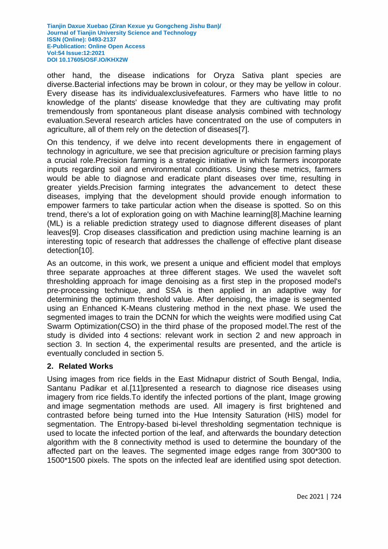
In recent years, rice has become one of the world's most significant food crops, providing the major source of nutrition for more than 2.7 billion people throughout the globe.Identifying Oryza Sativa diseases lately may have a major effect on crop cultivation and, at the end, result in a lower crop yield. There are various diseases that can impact the growth of Oryza Sativa, of whichBrown Spot,Bacterial leaf blight, and Leaf blast [5], are the main concern which are shown in Figure 1, 2,&Figure
respectively.
Bacterial leaf blight disease is developed by Xanthomonasory zaepvoryzaeth, which attempts to drop shrubs and leaves to dry and yellowish. Most of this disease is found in the plant leaf. The infected leaves turn out to be greyish green and furl in the younger years. [4].Leaf brown spot disease is a fungus called Cochlio bolusmiya beanus. Large spots on the leaves, which cover the entire leaf, are a sign that it's a problem. [5]. Magnaporthe oryzae, a fungus, causes leaf blast disease, which damages the entire plant. When blast spores are present, it's more likely to occur. During the early phases, white or gray-green dots with dark green brims appear. When the grazes are mature, they become elliptical or stick-shaped [6].
In order to prevent the illness from spreading to the surrounding plant parts and even to nearby plants, it's vital to discover it and take the appropriate precautions.On the
Figure 1: Bacterial Leaf Blight Figure 2: Brown Spot Figure 3: Leaf Blast
Tianjin Daxue Xuebao (Ziran Kexue yu Gongcheng Jishu Ban)/ Journal of Tianjin University Science and Technology ISSN (Online): 0493-2137 E-Publication: Online Open Access Vol:54 Issue:12:2021 DOI 10.17605/OSF.IO/KHX2W
Dec 2021 | 724
other hand, the disease indications for Oryza Sativa plant species are diverse.Bacterial infections may be brown in colour, or they may be yellow in colour. Every disease has its individualexclusivefeatures. Farmers who have little to no knowledge of the plants' disease knowledge that they are cultivating may profit tremendously from spontaneous plant disease analysis combined with technology evaluation.Several research articles have concentrated on the use of computers in agriculture, all of them rely on the detection of diseases[7].
On this tendency, if we delve into recent developments there in engagement of technology in agriculture, we see that precision agriculture or precision farming plays a crucial role.Precision farming is a strategic initiative in which farmers incorporate inputs regarding soil and environmental conditions. Using these metrics, farmers would be able to diagnose and eradicate plant diseases over time, resulting in greater yields.Precision farming integrates the advancement to detect these diseases, implying that the development should provide enough information to empower farmers to take particular action when the disease is spotted. So on this trend, there's a lot of exploration going on with Machine learning[8].Machine learning (ML) is a reliable prediction strategy used to diagnose different diseases of plant leaves[9]. Crop diseases classification and prediction using machine learning is an interesting topic of research that addresses the challenge of effective plant disease detection[10].
As an outcome, in this work, we present a unique and efficient model that employs three separate approaches at three different stages. We used the wavelet soft thresholding approach for image denoising as a first step in the proposed model's pre-processing technique, and SSA is then applied in an adaptive way for determining the optimum threshold value. After denoising, the image is segmented using an Enhanced K-Means clustering method in the next phase. We used the segmented images to train the DCNN for which the weights were modified using Cat Swarm Optimization(CSO) in the third phase of the proposed model.The rest of the study is divided into 4 sections: relevant work in section 2 and new approach in section 3. In section 4, the experimental results are presented, and the article is eventually concluded in section 5.
2. Related Works
Using images from rice fields in the East Midnapur district of South Bengal, India, Santanu Padikar et al.[11]presented a research to diagnose rice diseases using imagery from rice fields.To identify the infected portions of the plant, Image growing and image segmentation methods are used. All imagery is first brightened and contrasted before being turned into the Hue Intensity Saturation (HIS) model for segmentation. The Entropy-based bi-level thresholding segmentation technique is used to locate the infected portion of the leaf, and afterwards the boundary detection algorithm with the 8 connectivity method is used to determine the boundary of the affected part on the leaves. The segmented image edges range from 300*300 to 1500*1500 pixels. The spots on the infected leaf are identified using spot detection.
Tianjin Daxue Xuebao (Ziran Kexue yu Gongcheng Jishu Ban)/ Journal of Tianjin University Science and Technology ISSN (Online): 0493-2137 E-Publication: Online Open Access Vol:54 Issue:12:2021 DOI 10.17605/OSF.IO/KHX2W
Dec 2021 | 725
For classification, a self-organizing map (SOM) neural network is used. The study attained 92 percent accuracy by using the spots on the images for classification.
P. Sanyal et al. [12] recommended a study using Rice leaf blast and Brown spot as the research object to diagnose the rice life infection. Throughout this article, 400 samples were captured, with 80 percent of them being used for training and the remaining 20% being used for testing. The feature vector was computed by considering the 7*7 neighbourhood by each pixel in the image. The Multilayer perceptron classifier was given 70 hidden nodes of colour features and 40 hidden nodes of texture features, and the results obtained correlates from both colour and texture featuring MLPs, and statistical method including its identification ended in 89.26 % accuracy.
Santanu Phadikar et al.[13] used the Fermi energy-based region extraction technique to overcome the constraint of choosing a threshold value.They concentrated on the Oryza Sativa diseases blast, rot, brown spot, and blight. The researchers used a genetic algorithm to determine the shape of the diseased leaf area. The primary advantage of the proposed model is that it eliminates the need for gain calculation, which helps to reduce computing complexity. A ten-fold cross validation is used to assess the efficacy of the proposed method, which outperforms other techniques such as Naive Bayes, SMO, and Bagging.
Rice disease imagery were obtained from the International Rice Research Institute in Los Banos, Laguna, Philippines, and a study using backpropagation artificial neural network was submitted by John William ORILLO et al. [14]. The diseases brown Spot, rice blast, and bacterial leaf blight were chosen as the original study target. The images are improved throughout this research by doing noise reduction and contrast improvements, as well as being converted from RGB to HSV (Hue Saturation-Value) colour space. The contrast of the images is altered by using Otsu's approach. The processed images are converted to binary level images using the thresholding masking procedure, and then noise is removed employing Blob extraction. The infection is extracted using the A-colour plane after the segmented leaf image is transformed to LAB colour space.
The Heilongjiang Academy of Land Reclamation Sciences in China provided imagery to Yang Lu et al. [5]. The ailments studied were brown spot, rice blast, false smut, bakanae, sheath blight, sheath rot, bacterial sheath, seedling blight, bacterial wilt, and bacterial leaf blight. The author gathered 500 pictures of 10 different rice diseases from multiple sources for this research. All images were reduced to 512*512 to decrease the time complexity, and afterwards the ZCA whitening procedure is used to eliminate the similarity of datasets. The pictures are also labelled with ten different types of rice diseases. An image patch is created along with the corresponding feature map using the Pre-processing procedure and randomly choosing 10000 12*12 patches from the 500 images. Along with the corresponding feature map, an image patch is generated. The hierarchical architecture of CNN is suggested in this paper, which includes three Convolutional layers for extracting low-level and high-level features, a Stochastic pooling layer for
Tianjin Daxue Xuebao (Ziran Kexue yu Gongcheng Jishu Ban)/ Journal of Tianjin University Science and Technology ISSN (Online): 0493-2137 E-Publication: Online Open Access Vol:54 Issue:12:2021 DOI 10.17605/OSF.IO/KHX2W
Dec 2021 | 726
reducing variance, and softmax regression for multiclass classification. They used a supervised learning algorithm to train a network. According to the findings, when using the 10-fold cross-validation approach to train and test, stochastic pooling obtained 95.48 percent better recognition performance than mean pooling, max pooling, and stochastic pooling. The researchers assessed with recognition performance of various convolutional filters of sizes 5*5,9*9,16*16, and 32*32, with the results indicating that the 16*16 filter performed best with 93.29 percent. The suggested convolutional neural network (CNN) reached 95 percent accuracy when compared to the BP Method, support vector machine (SVM), and particle swarm optimization (PSO) results.
Chia-Lin Chung et al. [15] focused on bakanae disease, a seed-borne Oryza Sativa disease. The research primary goal was to use machine vision to differentiate between healthy and diseased seedlings. The best parameters for the SVM classifier were chosen using a genetic algorithm, and the classifier had an accuracy of 87.9% in distinguishing between healthy and unhealthy seedlings.
Shampa Sengupta et al. [16] researched on Oryza Sativa diseases such as rice blast, sheath rot, leaf brown spot, and bacterial blight. The primary research goal was to develop an incremental classifier that helps in reducing the time complexity of the classification system by extracting data from the old classifier and combining it with new data; doing so may help in reducing the time complexity in training the classifier as well as increasing the classifier's performance. An incremental rule-based classification system is designed using the particle swarm optimization technique and association rule mining.
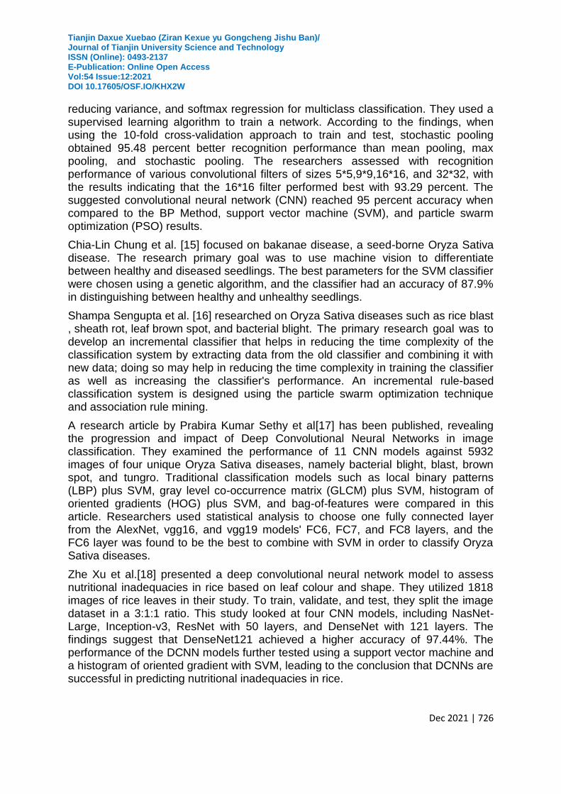
A research article by Prabira Kumar Sethy et al[17] has been published, revealing the progression and impact of Deep Convolutional Neural Networks in image classification. They examined the performance of 11 CNN models against 5932 images of four unique Oryza Sativa diseases, namely bacterial blight, blast, brown spot, and tungro. Traditional classification models such as local binary patterns (LBP) plus SVM, gray level co-occurrence matrix (GLCM) plus SVM, histogram of oriented gradients (HOG) plus SVM, and bag-of-features were compared in this article. Researchers used statistical analysis to choose one fully connected layer from the AlexNet, vgg16, and vgg19 models' FC6, FC7, and FC8 layers, and the FC6 layer was found to be the best to combine with SVM in order to classify Oryza Sativa diseases.
Zhe Xu et al.[18] presented a deep convolutional neural network model to assess nutritional inadequacies in rice based on leaf colour and shape. They utilized 1818 images of rice leaves in their study. To train, validate, and test, they split the image dataset in a 3:1:1 ratio. This study looked at four CNN models, including NasNet-Large, Inception-v3, ResNet with 50 layers, and DenseNet with 121 layers. The findings suggest that DenseNet121 achieved a higher accuracy of 97.44%. The performance of the DCNN models further tested using a support vector machine and a histogram of oriented gradient with SVM, leading to the conclusion that DCNNs are successful in predicting nutritional inadequacies in rice.
Tianjin Daxue Xuebao (Ziran Kexue yu Gongcheng Jishu Ban)/ Journal of Tianjin University Science and Technology ISSN (Online): 0493-2137 E-Publication: Online Open Access Vol:54 Issue:12:2021 DOI 10.17605/OSF.IO/KHX2W
Dec 2021 | 727
I V Arinichev et al.[19]Presented a research paper applying convolutional neural net- works to identify and categorize rice fungal infections. They used a publicly available dataset [20]and also obtained some images from an online source for their research. They removed Rice Hispa illnesses from the overall dataset since they are not common in Russia, and they trained and validated the model using 4278 images from three classes. They tested four models in this study: SqueezeNeq-1.0, DenseNet- 121, GoogleNet, and ResNet-18, and found that DenseNet-121 achieved 95% accuracy, which was the best among the other models.
Some image processing techniques and machine learning classifiers that are compatible with the defining evidence of Oryza Sativa plant disease have been examined[21].Researchers observed that majority of the research was centred around these two diseases on i.e. Rice Blast or Brown Spot. K-Means clustering was formerly believed to be the most widely utilised image segmentation method.
3. Proposed Solution
3.1 Overview
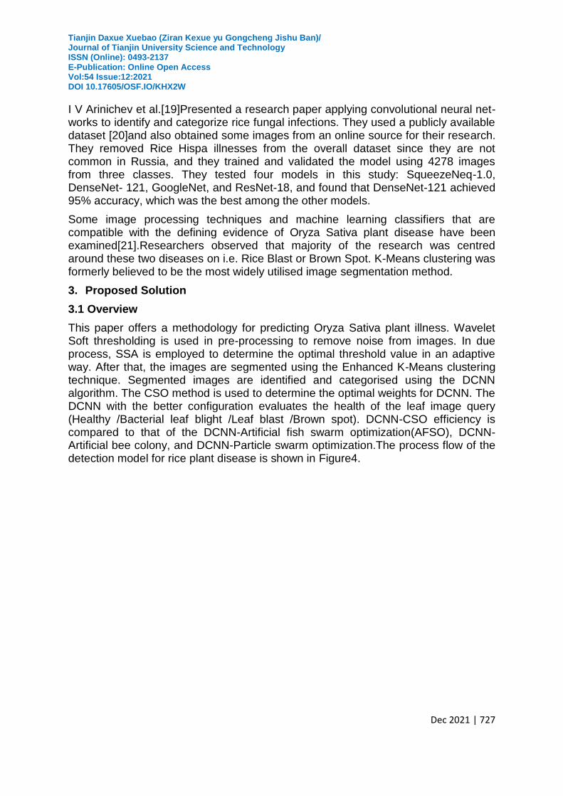
This paper offers a methodology for predicting Oryza Sativa plant illness. Wavelet Soft thresholding is used in pre-processing to remove noise from images. In due process, SSA is employed to determine the optimal threshold value in an adaptive way. After that, the images are segmented using the Enhanced K-Means clustering technique. Segmented images are identified and categorised using the DCNN algorithm. The CSO method is used to determine the optimal weights for DCNN. The DCNN with the better configuration evaluates the health of the leaf image query (Healthy /Bacterial leaf blight /Leaf blast /Brown spot). DCNN-CSO efficiency is compared to that of the DCNN-Artificial fish swarm optimization(AFSO), DCNN-Artificial bee colony, and DCNN-Particle swarm optimization.The process flow of the detection model for rice plant disease is shown in Figure4.
Tianjin Daxue Xuebao (Ziran Kexue yu Gongcheng Jishu Ban)/ Journal of Tianjin University Science and Technology ISSN (Online): 0493-2137 E-Publication: Online Open Access Vol:54 Issue:12:2021 DOI 10.17605/OSF.IO/KHX2W
Dec 2021 | 728
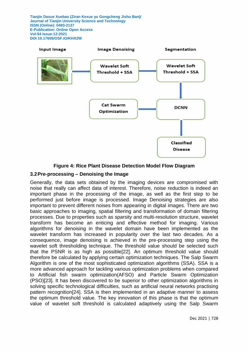
Figure 4: Rice Plant Disease Detection Model Flow Diagram
3.2 Pre-processing – Denoising the Image
Generally, the data sets obtained by the imaging devices are compromised with noise that really can affect data of interest. Therefore, noise reduction is indeed an important phase in the processing of the image, as well as the first step to be performed just before image is processed. Image Denoising strategies are also important to prevent different noises from appearing in digital images. There are two basic approaches to imaging, spatial filtering and transformation of domain filtering processes. Due to properties such as sparsity and multi-resolution structure, wavelet transform has become an enticing and effective method for imaging. Various algorithms for denoising in the wavelet domain have been implemented as the wavelet transform has increased in popularity over the last two decades. As a consequence, image denoising is achieved in the pre-processing step using the wavelet soft thresholding technique. The threshold value should be selected such that the PSNR is as high as possible[22]. An optimum threshold value should therefore be calculated by applying certain optimization techniques. The Salp Swarm Algorithm is one of the most sophisticated optimization algorithms (SSA). SSA is a more advanced approach for tackling various optimization problems when compared to Artificial fish swarm optimization(AFSO) and Particle Swarm Optimization (PSO)[23]. It has been discovered to be superior to other optimization algorithms in solving specific technological difficulties, such as artificial neural networks practising pattern recognition[24]. SSA is then implemented in an adaptive manner to assess the optimum threshold value. The key innovation of this phase is that the optimum value of wavelet soft threshold is calculated adaptively using the Salp Swarm
Tianjin Daxue Xuebao (Ziran Kexue yu Gongcheng Jishu Ban)/ Journal of Tianjin University Science and Technology ISSN (Online): 0493-2137 E-Publication: Online Open Access Vol:54 Issue:12:2021 DOI 10.17605/OSF.IO/KHX2W
Dec 2021 | 729
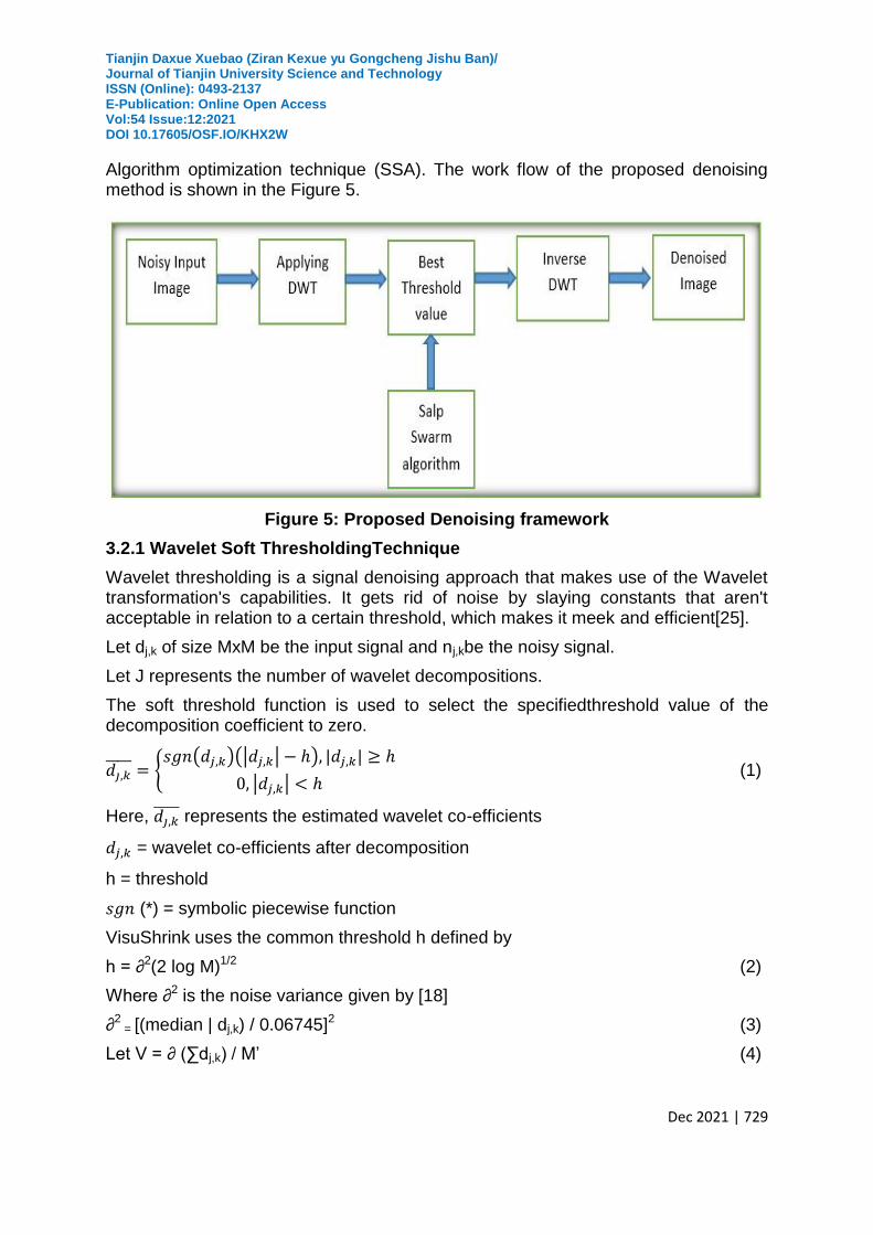
Algorithm optimization technique (SSA). The work flow of the proposed denoising method is shown in the Figure 5.
Figure 5: Proposed Denoising framework
3.2.1 Wavelet Soft ThresholdingTechnique
Wavelet thresholding is a signal denoising approach that makes use of the Wavelet transformation's capabilities. It gets rid of noise by slaying constants that aren't acceptable in relation to a certain threshold, which makes it meek and efficient[25].
Let dj,k of size MxM be the input signal and nj,kbe the noisy signal.
Let J represents the number of wavelet decompositions.
The soft threshold function is used to select the specifiedthreshold value of the decomposition coefficient to zero.
{
( )(| | )
| | (1)
Here, represents the estimated wavelet co-efficients
= wavelet co-efficients after decomposition
h = threshold
(*) = symbolic piecewise function
VisuShrink uses the common threshold h defined by
h = ∂2(2 log M)1/2 (2)
Where ∂2 is the noise variance given by [18]
∂2 = [(median | dj,k) / 0.06745]2 (3)
Let V = ∂ (∑dj,k) / M’ (4)

Tianjin Daxue Xuebao (Ziran Kexue yu Gongcheng Jishu Ban)/ Journal of Tianjin University Science and Technology ISSN (Online): 0493-2137 E-Publication: Online Open Access Vol:54 Issue:12:2021 DOI 10.17605/OSF.IO/KHX2W
Dec 2021 | 730
Where M’ = M / 2k, k=1,2,....J
The PSNR value of the denoised image is given by
(5)
Where MSE is the Mean Square Error calculated by taking the average of the squared strength of the actual (input) image and the denoised image.
Then the fitness function for SSA is derived by
Fi = maximum (V + PSNR, V-PSNR) (6)
In this function, the wavelet coefficients are selected such that fitness function returns the maximum value of V+PSNR or V-PSNR.
3.2.2 SSA for optimum threshold Estimation
SSA is used to adaptively evaluate the best threshold value. The selection of the threshold value should be such that the PSNR value is maximum [26]. The salp is classified as a member of the Salpidae family.The SSA is centered on the salp’s swarming behaviour.They are capable of creating mutual manacles in the wake of rummaging behaviour in deep seas. This activity connects salps to gain more kinetic energy in the search of a food source.The salp in the SSA algorithm is divided into two groups, each of which is based on the followers and representatives. In the chain, the leader salp is at the top, and the followers follow him. Many authors attribute about them as "followers" or "links."Leader salp supports the way and movement of the party while supporters use the other categories [27][28].
Figure 6:Structure of Salp chain
The locationtrajectory of everysalp is defined for examining and dimensional space, where is number of choice variables. The earlypopulace of SSO contains N
salp’s and d magnitudes. The position vector of the salps is represented by N×d dimensional matrix which is represented by the below equation,
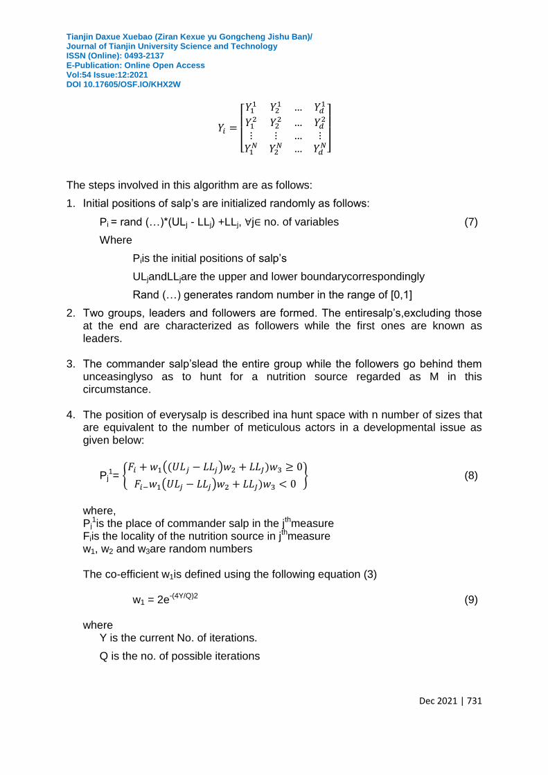
Tianjin Daxue Xuebao (Ziran Kexue yu Gongcheng Jishu Ban)/ Journal of Tianjin University Science and Technology ISSN (Online): 0493-2137 E-Publication: Online Open Access Vol:54 Issue:12:2021 DOI 10.17605/OSF.IO/KHX2W
Dec 2021 | 731
[
]
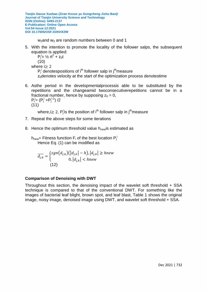
The steps involved in this algorithm are as follows:
1. Initial positions of salp’s are initialized randomly as follows:
Pi = rand (…)*(ULj - LLj) +LLj, ∀j∈ no. of variables (7)
Where
Piis the initial positions of salp’s
ULjandLLjare the upper and lower boundarycorrespondingly
Rand (…) generates random number in the range of [0,1]
2. Two groups, leaders and followers are formed. The entiresalp’s,excluding those at the end are characterized as followers while the first ones are known as leaders.
3. The commander salp’slead the entire group while the followers go behind them unceasinglyso as to hunt for a nutrition source regarded as M in this circumstance.
4. The position of everysalp is described ina hunt space with n number of sizes that
are equivalent to the number of meticulous actors in a developmental issue as given below:
Pj1= {
( )
( ) } (8)
where, Pj
1is the place of commander salp in the jthmeasure Fiis the locality of the nutrition source in jthmeasure w1, w2 and w3are random numbers
The co-efficient w1is defined using the following equation (3)
w1 = 2e-(4Y/Q)2 (9) where
Y is the current No. of iterations.
Q is the no. of possible iterations
Tianjin Daxue Xuebao (Ziran Kexue yu Gongcheng Jishu Ban)/ Journal of Tianjin University Science and Technology ISSN (Online): 0493-2137 E-Publication: Online Open Access Vol:54 Issue:12:2021 DOI 10.17605/OSF.IO/KHX2W
Dec 2021 | 732
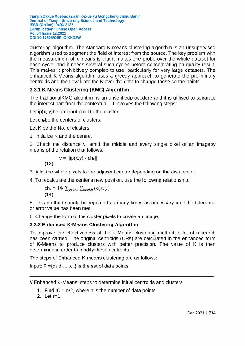
w2and w3 are random numbers between 0 and 1
5. With the intention to promote the locality of the follower salps, the subsequent equation is applied: Pj
i= ½ rt2 + z0t (10)
where i Pj
i denotespositions of ith follower salp in jthmeasure z0denotes velocity at the start of the optimization process denotestime
6. Asthe period in the developmentalprocessis able to be substituted by the
repetitions and the changeamid twoconsecutiverepetitions cannot be in a fractional number, hence by supposing z0 = 0, Pj
i= (Pji +Pj
i-1) /2 (11)
where,i , Pjiis the position of ith follower salp in jthmeasure
7. Repeat the above steps for some iterations
8. Hence the optimum threshold value hnewis estimated as
hnew= Fitness function Fi of the best location Pji
Hence Eq. (1) can be modified as
{
( )(| | ) | |
| |
(12)
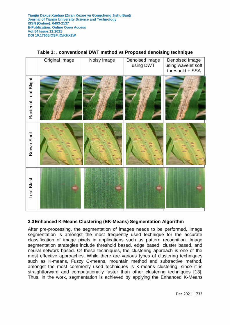
Comparison of Denoising with DWT
Throughout this section, the denoising impact of the wavelet soft threshold + SSA technique is compared to that of the conventional DWT. For something like the images of bacterial leaf blight, brown spot, and leaf blast, Table 1 shows the original image, noisy image, denoised image using DWT, and wavelet soft threshold + SSA.
Tianjin Daxue Xuebao (Ziran Kexue yu Gongcheng Jishu Ban)/ Journal of Tianjin University Science and Technology ISSN (Online): 0493-2137 E-Publication: Online Open Access Vol:54 Issue:12:2021 DOI 10.17605/OSF.IO/KHX2W
Dec 2021 | 733
Table 1: . conventional DWT method vs Proposed denoising technique
Original Image Noisy Image Denoised image using DWT
Denoised Image using wavelet soft threshold + SSA
Ba
cte
ria
l L
ea
f B
light
Bro
wn
Spo
t
Le
af B
last
3.3 Enhanced K-Means Clustering (EK-Means) Segmentation Algorithm
After pre-processing, the segmentation of images needs to be performed. Image segmentation is amongst the most frequently used technique for the accurate classification of image pixels in applications such as pattern recognition. Image segmentation strategies include threshold based, edge based, cluster based, and neural network based. Of these techniques, the clustering approach is one of the most effective approaches. While there are various types of clustering techniques such as K-means, Fuzzy C-means, mountain method and subtractive method, amongst the most commonly used techniques is K-means clustering, since it is straightforward and computationally faster than other clustering techniques [13]. Thus, in the work, segmentation is achieved by applying the Enhanced K-Means
Tianjin Daxue Xuebao (Ziran Kexue yu Gongcheng Jishu Ban)/ Journal of Tianjin University Science and Technology ISSN (Online): 0493-2137 E-Publication: Online Open Access Vol:54 Issue:12:2021 DOI 10.17605/OSF.IO/KHX2W
Dec 2021 | 734
clustering algorithm. The standard K-means clustering algorithm is an unsupervised algorithm used to segment the field of interest from the source. The key problem with the measurement of k-means is that it makes one probe over the whole dataset for each cycle, and it needs several such cycles before concentrating on quality result. This makes it prohibitively complex to use, particularly for very large datasets. The enhanced K-Means algorithm uses a greedy approach to generate the preliminary centroids and then evaluate the K over the data to change those centre points.
3.3.1 K-Means Clustering (KMC) Algorithm
The traditionalKMC algorithm is an unverifiedprocedure and it is utilised to separate the interest part from the contextual. It involves the following steps:
Let ip(x, y)be an input pixel to the cluster
Let chkbe the centers of clusters.
Let K be the No. of clusters
1. Initialize K and the centre.
2. Check the distance v, amid the middle and every single pixel of an imageby means of the relation that follows.
v = ||ip(x,y) - chk|| (13)
3. Allot the whole pixels to the adjacent centre depending on the distance d.
4. To recalculate the center's new position, use the following relationship:
chk = 1/k ∑ ∑
(14)
5. This method should be repeated as many times as necessary until the tolerance or error value has been met.
6. Change the form of the cluster pixels to create an image.
3.3.2 Enhanced K-Means Clustering Algorithm
To improve the effectiveness of the K-Means clustering method, a lot of research has been carried. The original centroids (CRs) are calculated in the enhanced form of K-Means to produce clusters with better precision. The value of K is then determined in order to modify these centroids.
The steps of Enhanced K-means clustering are as follows:
Input: P ={d1,d2,....dn} is the set of data points.
___________________________________________________________________
// Enhanced K-Means: steps to determine initial centroids and clusters
1. Find IC = n/2, where n is the number of data points 2. Let r=1
Tianjin Daxue Xuebao (Ziran Kexue yu Gongcheng Jishu Ban)/ Journal of Tianjin University Science and Technology ISSN (Online): 0493-2137 E-Publication: Online Open Access Vol:54 Issue:12:2021 DOI 10.17605/OSF.IO/KHX2W
Dec 2021 | 735
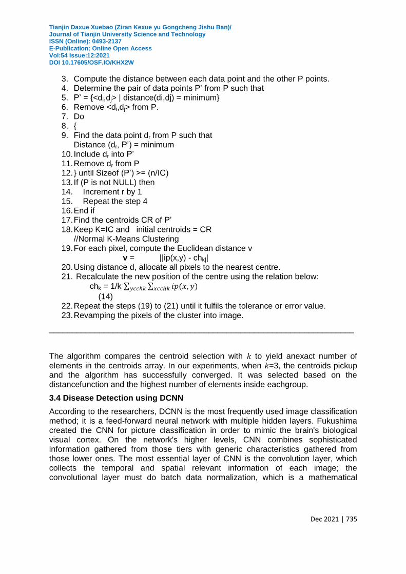
3. Compute the distance between each data point and the other P points. 4. Determine the pair of data points P’ from P such that 5. P’ = {<di,dj> | distance(di,dj) = minimum} 6. Remove <di,dj> from P. 7. Do 8. { 9. Find the data point dr from P such that
Distance (dr, P’) = minimum 10. Include dr into P’ 11. Remove dr from P 12. } until Sizeof (P’) >= (n/IC) 13. If (P is not NULL) then 14. Increment r by 1 15. Repeat the step 4 16. End if 17. Find the centroids CR of P’ 18. Keep K=IC and initial centroids = CR
//Normal K-Means Clustering 19. For each pixel, compute the Euclidean distance v
v = ||ip(x,y) - chk|| 20. Using distance d, allocate all pixels to the nearest centre. 21. Recalculate the new position of the centre using the relation below:
chk = 1/k ∑ ∑
(14) 22. Repeat the steps (19) to (21) until it fulfils the tolerance or error value. 23. Revamping the pixels of the cluster into image.
___________________________________________________________________
The algorithm compares the centroid selection with 𝑘 to yield anexact number of elements in the centroids array. In our experiments, when 𝑘=3, the centroids pickup and the algorithm has successfully converged. It was selected based on the distancefunction and the highest number of elements inside eachgroup.
3.4 Disease Detection using DCNN
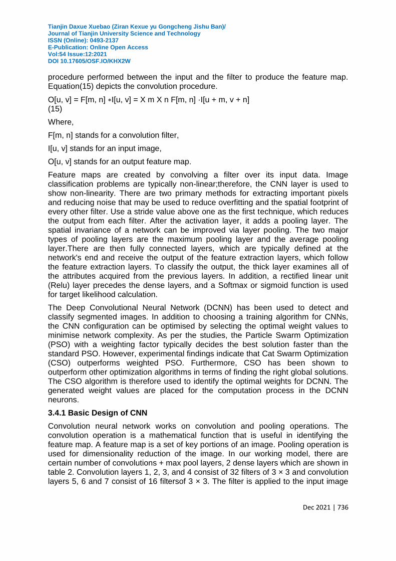
According to the researchers, DCNN is the most frequently used image classification method; it is a feed-forward neural network with multiple hidden layers. Fukushima created the CNN for picture classification in order to mimic the brain's biological visual cortex. On the network's higher levels, CNN combines sophisticated information gathered from those tiers with generic characteristics gathered from those lower ones. The most essential layer of CNN is the convolution layer, which collects the temporal and spatial relevant information of each image; the convolutional layer must do batch data normalization, which is a mathematical
Tianjin Daxue Xuebao (Ziran Kexue yu Gongcheng Jishu Ban)/ Journal of Tianjin University Science and Technology ISSN (Online): 0493-2137 E-Publication: Online Open Access Vol:54 Issue:12:2021 DOI 10.17605/OSF.IO/KHX2W
Dec 2021 | 736
procedure performed between the input and the filter to produce the feature map. Equation(15) depicts the convolution procedure.
O[u, v] = F[m, n] ∗I[u, v] = X m X n F[m, n] ·I[u + m, v + n] (15)
Where,
F[m, n] stands for a convolution filter,
I[u, v] stands for an input image,
O[u, v] stands for an output feature map.
Feature maps are created by convolving a filter over its input data. Image classification problems are typically non-linear;therefore, the CNN layer is used to show non-linearity. There are two primary methods for extracting important pixels and reducing noise that may be used to reduce overfitting and the spatial footprint of every other filter. Use a stride value above one as the first technique, which reduces the output from each filter. After the activation layer, it adds a pooling layer. The spatial invariance of a network can be improved via layer pooling. The two major types of pooling layers are the maximum pooling layer and the average pooling layer.There are then fully connected layers, which are typically defined at the network's end and receive the output of the feature extraction layers, which follow the feature extraction layers. To classify the output, the thick layer examines all of the attributes acquired from the previous layers. In addition, a rectified linear unit (Relu) layer precedes the dense layers, and a Softmax or sigmoid function is used for target likelihood calculation.
The Deep Convolutional Neural Network (DCNN) has been used to detect and classify segmented images. In addition to choosing a training algorithm for CNNs, the CNN configuration can be optimised by selecting the optimal weight values to minimise network complexity. As per the studies, the Particle Swarm Optimization (PSO) with a weighting factor typically decides the best solution faster than the standard PSO. However, experimental findings indicate that Cat Swarm Optimization (CSO) outperforms weighted PSO. Furthermore, CSO has been shown to outperform other optimization algorithms in terms of finding the right global solutions. The CSO algorithm is therefore used to identify the optimal weights for DCNN. The generated weight values are placed for the computation process in the DCNN neurons.
3.4.1 Basic Design of CNN
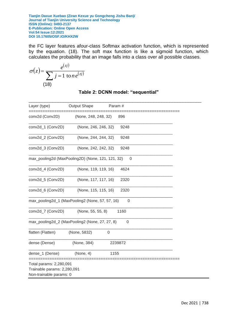
Convolution neural network works on convolution and pooling operations. The convolution operation is a mathematical function that is useful in identifying the feature map. A feature map is a set of key portions of an image. Pooling operation is used for dimensionality reduction of the image. In our working model, there are certain number of convolutions + max pool layers, 2 dense layers which are shown in table 2. Convolution layers 1, 2, 3, and 4 consist of 32 filters of 3 × 3 and convolution layers 5, 6 and 7 consist of 16 filtersof 3 × 3. The filter is applied to the input image
Tianjin Daxue Xuebao (Ziran Kexue yu Gongcheng Jishu Ban)/ Journal of Tianjin University Science and Technology ISSN (Online): 0493-2137 E-Publication: Online Open Access Vol:54 Issue:12:2021 DOI 10.17605/OSF.IO/KHX2W
Dec 2021 | 737
and identifies the image features such as Shape, edges and boundaries. When the filter is applied to the first 3 × 3 part of an input image, the features are equivalent or higher to the threshold value. The filter slides through the image horizontally and vertically and keeps on updating the features of the image. After applying the convolution operation, the output image is produced with 248 x 248 from equation (16).
112
S
PKNM
(16)
M is the output Shape, N is the input image Shape, K is the filter, P is the padding, and S is the stride of the output image.
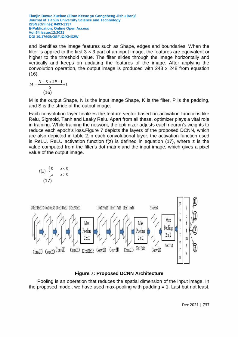
Each convolution layer finalizes the feature vector based on activation functions like Relu, Sigmoid, Tanh and Leaky Relu. Apart from all these, optimizer plays a vital role in training. While training the network, the optimizer adjusts each neuron's weights to reduce each epoch's loss.Figure 7 depicts the layers of the proposed DCNN, which are also depicted in table 2.In each convolutional layer, the activation function used is ReLU. ReLU activation function f(z) is defined in equation (17), where z is the value computed from the filter's dot matrix and the input image, which gives a pixel value of the output image.
0
00
zz
zzf
(17)
Figure 7: Proposed DCNN Architecture
Pooling is an operation that reduces the spatial dimension of the input image. In the proposed model, we have used max-pooling with padding = 1. Last but not least,
Tianjin Daxue Xuebao (Ziran Kexue yu Gongcheng Jishu Ban)/ Journal of Tianjin University Science and Technology ISSN (Online): 0493-2137 E-Publication: Online Open Access Vol:54 Issue:12:2021 DOI 10.17605/OSF.IO/KHX2W
Dec 2021 | 738
the FC layer features afour-class Softmax activation function, which is represented by the equation. (18). The soft max function is like a sigmoid function, which calculates the probability that an image falls into a class over all possible classes.
zj
zj
enj
ez
to1
(18)
Table 2: DCNN model: “sequential"
_________________________________________________________________ Layer (type) Output Shape Param #
=================================================================
conv2d (Conv2D) (None, 248, 248, 32) 896
_________________________________________________________________
conv2d_1 (Conv2D) (None, 246, 246, 32) 9248
_________________________________________________________________
conv2d_2 (Conv2D) (None, 244, 244, 32) 9248
_________________________________________________________________
conv2d_3 (Conv2D) (None, 242, 242, 32) 9248
_________________________________________________________________
max_pooling2d (MaxPooling2D) (None, 121, 121, 32) 0
_________________________________________________________________
conv2d_4 (Conv2D) (None, 119, 119, 16) 4624
_________________________________________________________________
conv2d_5 (Conv2D) (None, 117, 117, 16) 2320
_________________________________________________________________
conv2d_6 (Conv2D) (None, 115, 115, 16) 2320
_________________________________________________________________
max_pooling2d_1 (MaxPooling2 (None, 57, 57, 16) 0
_________________________________________________________________
conv2d_7 (Conv2D) (None, 55, 55, 8) 1160
_________________________________________________________________
max_pooling2d_2 (MaxPooling2 (None, 27, 27, 8) 0
_________________________________________________________________
flatten (Flatten) (None, 5832) 0
_________________________________________________________________
dense (Dense) (None, 384) 2239872
_________________________________________________________________
dense_1 (Dense) (None, 4) 1155
=================================================================
Total params: 2,280,091
Trainable params: 2,280,091
Non-trainable params: 0

Tianjin Daxue Xuebao (Ziran Kexue yu Gongcheng Jishu Ban)/ Journal of Tianjin University Science and Technology ISSN (Online): 0493-2137 E-Publication: Online Open Access Vol:54 Issue:12:2021 DOI 10.17605/OSF.IO/KHX2W
Dec 2021 | 739
3.5 Optimization of Weights using CSO For identifying the optimal weights for DCNN, Cat Swarm Optimization (CSO) algorithm is applied.The flow diagram for the proposed DCNN-CSO is shown in the figure 8.
3.5.1 CSO Algorithm
In CSO, primarily the amount of cats will be definite which is then used to resolve the issues. CSO comprises two sub-models: the seeking mode (SM) and the tracing mode (TM). Each cat has its individuallocation composed of M sizes, speeds for everysize, appropriateness value, which signifies the admittance of the cat to the appropriateness function and a flag to recognize whether the cat is in SM or TM. The lastresult would be the finestlocation in one of the cats because that CSO retains the finestresult till it touches the end of reiterations[29][30].
Seeking Mode (SM)
The sub-model is being used to simulate the cat's state, which includes relaxing, gazing about, and searching for a new place. Searching for a memory pool (SMP), searching for a selected dimension set (SRD), dimension to modify counts (CDC), and self-position consideration are the four key features discussed in SM (SPC). The amount of each cat's search memory, which identifies the points required by the cat, is determined using SMP. The cat will choose a point from the retention pool based on the late rubrics. As an example, the SM can be defined as follows:
If the aim of the appropriateness function is to discover the leastresolution, ,else . is the fitness value for all the candidate positions and is the probability of the ith candidate. SRD announces the mutative ratio for the designatedsizes. In SM, when a measurement if decided to change, the difference between the new and old value does not go outside of the SRD-defined range. CDC reveals how many sizes will be diverse. All of these elements play a vital role in the SM. SPC is a Boolean variable that determines if the cat's former residence will be one of the candidates for relocation.
Tracing Mode (TM)
TM is indeed a sub-model that depicts the cat's situation when attempting to achieve particular objectives. When a cat enters tracing mode, it transfers according to its unique velocities in each dimension. The following is a definition of the TM:
( )
Tianjin Daxue Xuebao (Ziran Kexue yu Gongcheng Jishu Ban)/ Journal of Tianjin University Science and Technology ISSN (Online): 0493-2137 E-Publication: Online Open Access Vol:54 Issue:12:2021 DOI 10.17605/OSF.IO/KHX2W
Dec 2021 | 740
is the location of the cat, Vk,d is the velocities update which has the
finestappropriateness value; is the location of cat k. is a scalar and is a
arbitrary value in the series of [0,1].
Procedure of CSO algorithm
To pool the two manners into the procedure, describe a mixture ratio (MR) of linkingSM and TM. When we study the actions of cats, we see that they apply most of the time when they are aware of resting. They move locations cautiously and gradually while resting, occasionally even stopping at the actual location. In order to signal this deed in CSO, we use searching mode in one manner or another. The CSO method may be divided into six steps, as shown below:
The action of running after objectives of cat is used forTM. Hence MR must be a minute value so as to assure that the cats use majority of the time in SM, just like the actual domain.
The CSO method may be divided into six steps, as shown below:
Step1:Generate N cats in the procedure, which is utilised to keep informed theirlocation
Step2:Arbitrarilyscatter the cats into the TM or SM and arbitrarily choose values, in-range of supremespeed, to the speeds of each cat. Then randomlychoose number of cats and fix them into TMbased on MR, and the remaining fix into SM.
Step3:Apply the locations of cats into the fitness function to determine each cat's fitness value, which represents our goal means principles, and keep the best cat in consideration. It's important to note that we're only interested in the location of the best cat (xbest) as it represents the highest resolution.
Step4:Transfer the cats based on their flags
If cat k is in SM,
Keep the cat to the SM procedure,
Else
Keepthe cat to the TMprocedure.
Step5: Re-select the number of cats and changethem into TMbased on MR, and thenfix the remaining cats into seeking mode.
Step6:Verify the closuresituation, if content, dismiss the program, and else repeat step 3 to step 5.

Tianjin Daxue Xuebao (Ziran Kexue yu Gongcheng Jishu Ban)/ Journal of Tianjin University Science and Technology ISSN (Online): 0493-2137 E-Publication: Online Open Access Vol:54 Issue:12:2021 DOI 10.17605/OSF.IO/KHX2W
Dec 2021 | 741
Figure 8: Flow diagram of proposed DCNN CSO
Tianjin Daxue Xuebao (Ziran Kexue yu Gongcheng Jishu Ban)/ Journal of Tianjin University Science and Technology ISSN (Online): 0493-2137 E-Publication: Online Open Access Vol:54 Issue:12:2021 DOI 10.17605/OSF.IO/KHX2W
Dec 2021 | 742
4. Experimental Results
In this research, we used a 2500-image dataset of four classes: Bacterial Leaf Blight, Leaf Blast, Brown Spot, and Healthy. We have split the dataset in 3:1:1 ratio for training, validation, and testing.
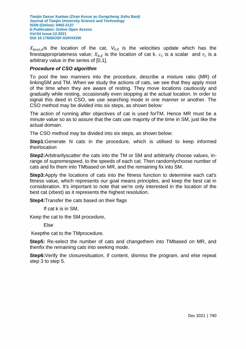
4.1 Results of Denoising& Segmentation
This section contains the results of segmented images containing various diseases. Figure 9 shows the input images along with the denoised and segmented images.
Figure 9: Results of the Segmented Images
Tianjin Daxue Xuebao (Ziran Kexue yu Gongcheng Jishu Ban)/ Journal of Tianjin University Science and Technology ISSN (Online): 0493-2137 E-Publication: Online Open Access Vol:54 Issue:12:2021 DOI 10.17605/OSF.IO/KHX2W
Dec 2021 | 743
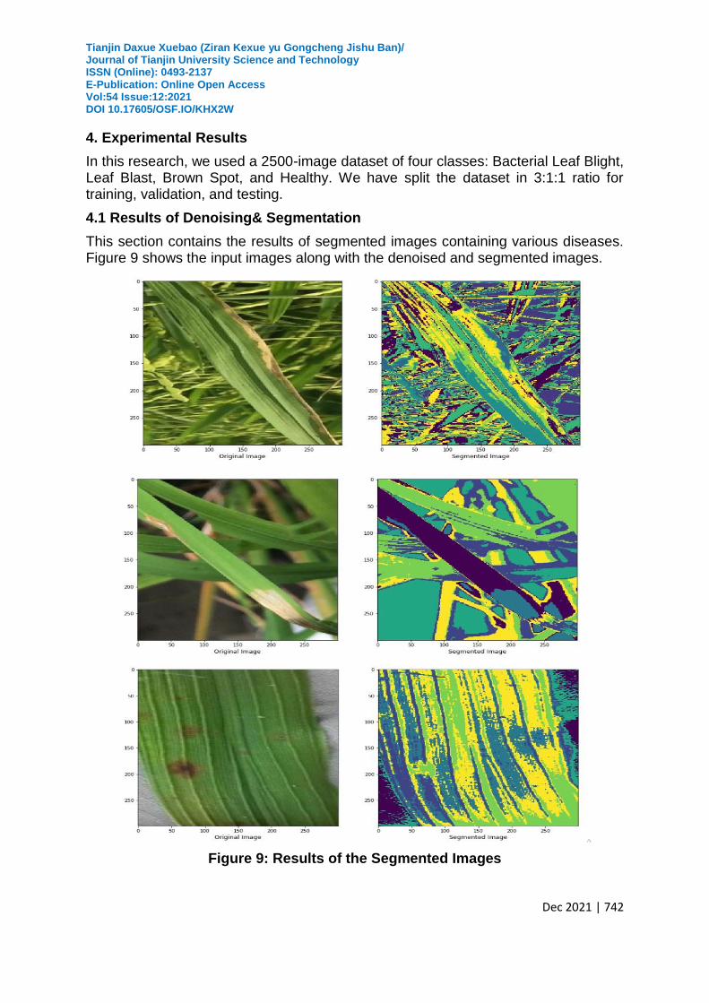
4.1.1 Comparison of proposed Denoising technique with DWT
Figure10compares output performance of the suggested wavelet soft threshold + SSA and the traditional DWT methods for denoising.
Figure 10: Graph showing PSNR values
4.1.2 Comparison of proposed Segmentation with Traditional approaches
The effectiveness of the suggested segmentation method is compared to that of the traditional K-Means segmentation methodology, which uses objective segmentation evaluation criteria such as the Jacquard Coefficient and Volumetric similarity.The standardmetric values range from -1 to 1, and the standard criterion is near to 1. The better the segmentation technique, the closer it is to value 1. This model is clearly more efficient than the standard K-Means, based on the results obtained.
(21)
| |
(22)
Where, , |
|, |
|,
= non zero-pixel element in Original image
= non zero-pixel element is Segmented image
0
5
10
15
20
25
30
35
40
45
30-50 30-40 30-40
Blast Bacterial Leaf Blight Brown spot
PSNR Comparision
Denoising method Denoising method
Tianjin Daxue Xuebao (Ziran Kexue yu Gongcheng Jishu Ban)/ Journal of Tianjin University Science and Technology ISSN (Online): 0493-2137 E-Publication: Online Open Access Vol:54 Issue:12:2021 DOI 10.17605/OSF.IO/KHX2W
Dec 2021 | 744
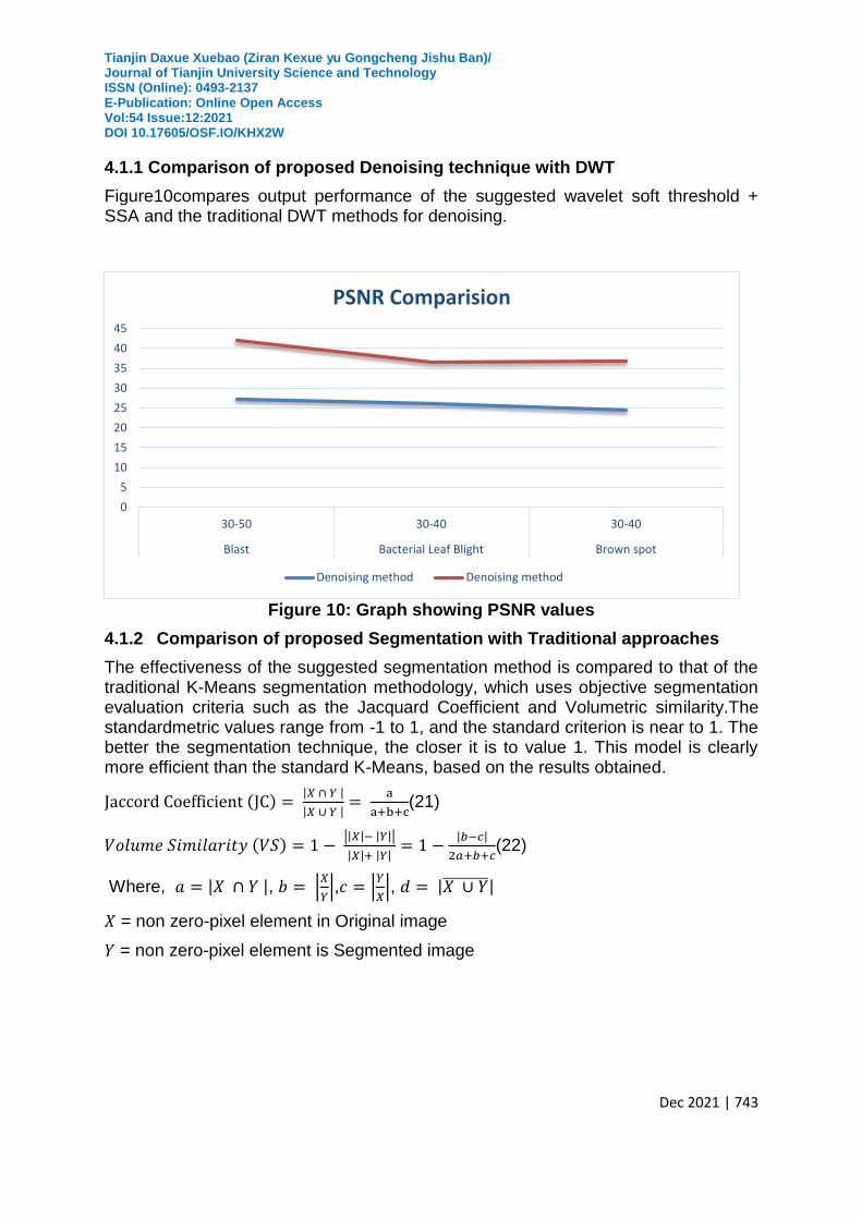
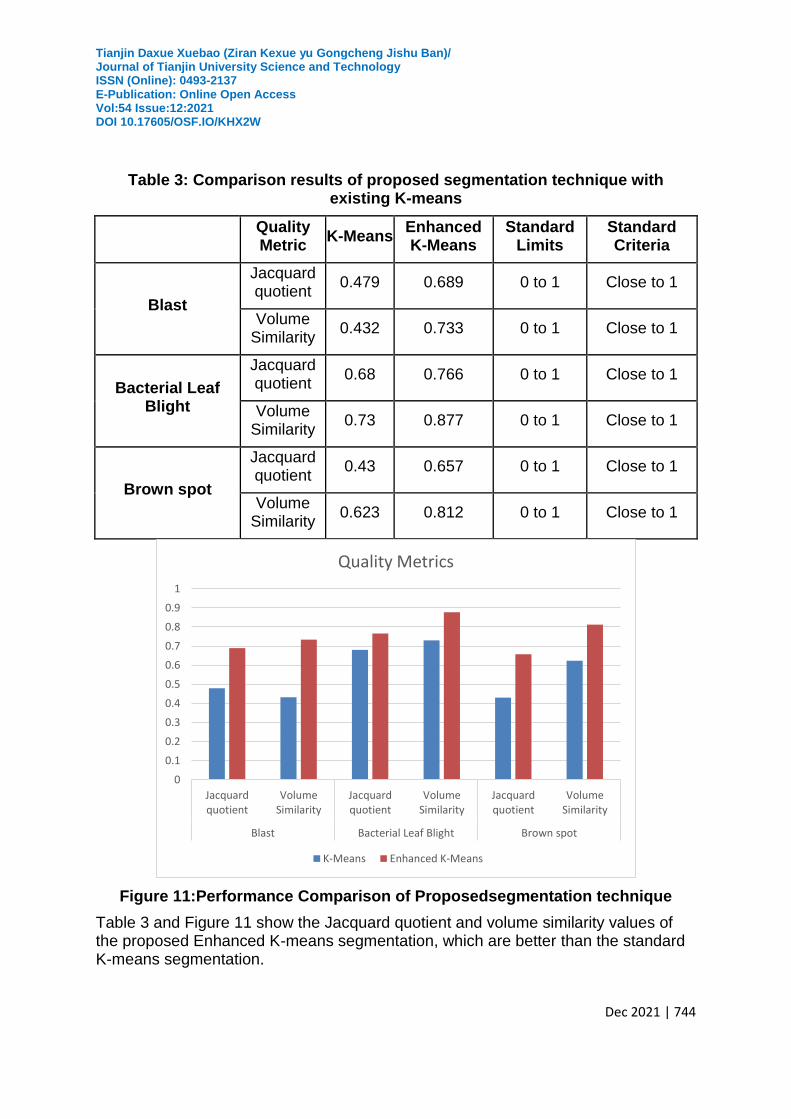
Table 3: Comparison results of proposed segmentation technique with existing K-means
Quality Metric
K-Means Enhanced K-Means
Standard Limits
Standard Criteria
Blast
Jacquard quotient
0.479 0.689 0 to 1 Close to 1
Volume Similarity
0.432 0.733 0 to 1 Close to 1
Bacterial Leaf Blight
Jacquard quotient
0.68 0.766 0 to 1 Close to 1
Volume Similarity
0.73 0.877 0 to 1 Close to 1
Brown spot
Jacquard quotient
0.43 0.657 0 to 1 Close to 1
Volume Similarity
0.623 0.812 0 to 1 Close to 1
Figure 11:Performance Comparison of Proposedsegmentation technique
Table 3 and Figure 11 show the Jacquard quotient and volume similarity values of the proposed Enhanced K-means segmentation, which are better than the standard K-means segmentation.
0
0.1
0.2
0.3
0.4
0.5
0.6
0.7
0.8
0.9
1
Jacquardquotient
VolumeSimilarity
Jacquardquotient
VolumeSimilarity
Jacquardquotient
VolumeSimilarity
Blast Bacterial Leaf Blight Brown spot
Quality Metrics
K-Means Enhanced K-Means
Tianjin Daxue Xuebao (Ziran Kexue yu Gongcheng Jishu Ban)/ Journal of Tianjin University Science and Technology ISSN (Online): 0493-2137 E-Publication: Online Open Access Vol:54 Issue:12:2021 DOI 10.17605/OSF.IO/KHX2W
Dec 2021 | 745
4.2 Comparison of Classification Accuracy with other Optimization Techniques
The findings of the DCNN classifier with CSO optimization are compared to the DCNN-AFSO, DCNN-ABC, and DCNN-PSO approaches in this article. The weights in DCNN have been optimised using Artificial fish swarm optimization(AFSO), Artificial bee colony (ABC) algorithm, and Particle swarm (PSO) optimization techniques in each of these techniques.
Table 4: Comparison results of DCNN model with other optimization techniques
Performance Measure DCNN-CSO DCNN-AFSO DCNN-ABC DCNN-PSO
Accuracy 0.969 0.786 0.814 0.587
Sensitivity 0.811 0.642 0.724 0.453
Specificity 0.984 0.863 0.883 0.671
PPV 0.951 0.842 0.832 0.653
NPV 0.854 0.863 0.880 0.621
MCC 0.878 0.713 0.761 0.485
F1-score 0.901 0.726 0.763 0.493
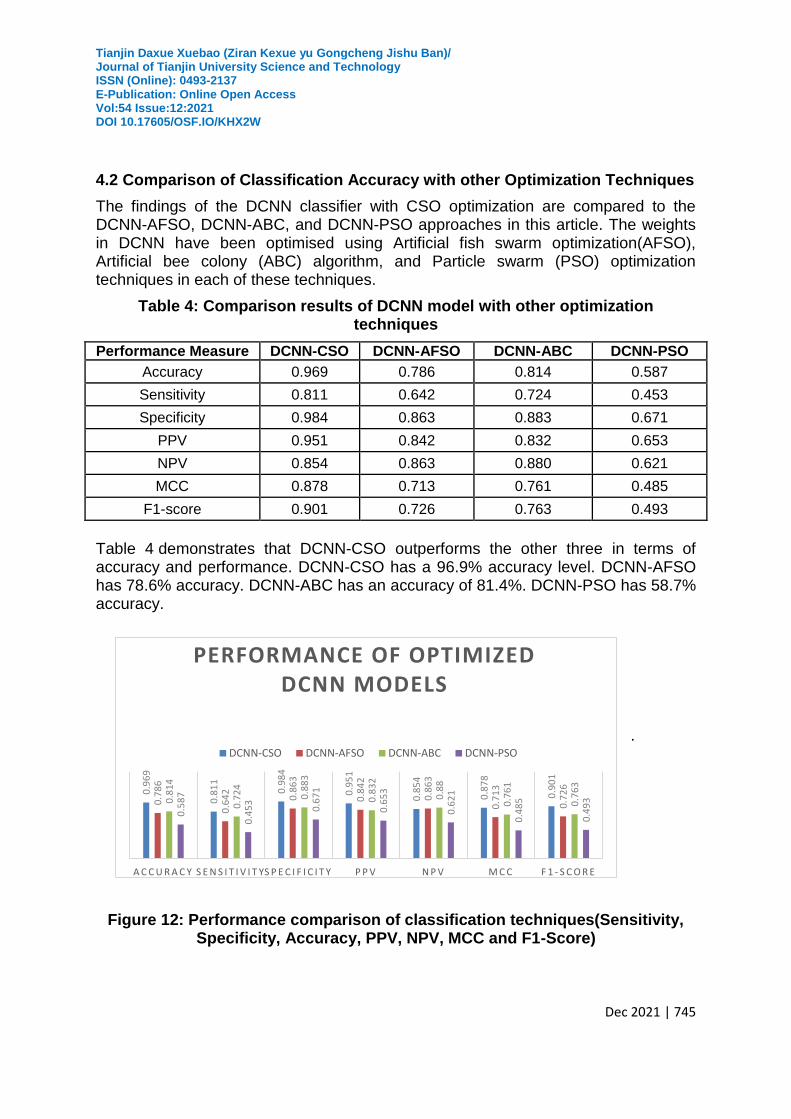
Table 4 demonstrates that DCNN-CSO outperforms the other three in terms of accuracy and performance. DCNN-CSO has a 96.9% accuracy level. DCNN-AFSO has 78.6% accuracy. DCNN-ABC has an accuracy of 81.4%. DCNN-PSO has 58.7% accuracy.
.
Figure 12: Performance comparison of classification techniques(Sensitivity, Specificity, Accuracy, PPV, NPV, MCC and F1-Score)
0.9
69
0.8
11
0.9
84
0.9
51
0.8
54
0.8
78
0.9
01
0.7
86
0.6
42
0.8
63
0.8
42
0.8
63
0.7
13
0.7
26
0.8
14
0.7
24
0.8
83
0.8
32
0.8
8
0.7
61
0.7
63
0.5
87
0.4
53
0.6
71
0.6
53
0.6
21
0.4
85
0.4
93
A C C U R A C Y S E N S I T I V I T Y S P E C I F I C I T Y P P V N P V M C C F 1 - S C O R E
PERFORMANCE OF OPTIMIZED DCNN MODELS
DCNN-CSO DCNN-AFSO DCNN-ABC DCNN-PSO
Tianjin Daxue Xuebao (Ziran Kexue yu Gongcheng Jishu Ban)/ Journal of Tianjin University Science and Technology ISSN (Online): 0493-2137 E-Publication: Online Open Access Vol:54 Issue:12:2021 DOI 10.17605/OSF.IO/KHX2W
Dec 2021 | 746
Figure 12illustrate the classification accuracy results of DCNN-CSO against DCNN-AFSO, DCNN-ABC, and DCNN-PSO. DCNN-CSO has the highest sensitivity i.e., 81.1%, DCNN-AFSO has 64.2% sensitivity, DCNN-ABC has 72.4% sensitivity, and DCNN-PSO has 45.3% sensitivity.
DCNN-CSO has a specificity of about 98.4%, DCNN-AFSO has a specificity of about 86.3%, DCNN-ABC has a specificity of about 88.3%, and DCNN-PSO has a specificity of about 67.1%. DCNN-CSO has a PPV of around 95.1%, DCNN-AFSO has a PPV of around 84.2%, DCNN-ABC has a PPV of around 83.2%, and DCNN-PSO has a PPV of around 65.3%.
Figure 12 indicates that DCNN-CSO has the highest MCC score of around 87.8%, while DCNN-AFSO has an MCC of around 71.3%, DCNN-ABC has an MCC of around 76.1%, and DCNN-PSO has an MCC of around 49.5%. Similarly, the DCNN-CSO has the highest F1-score of around 90.1%, the DCNN-AFSO has an F1-score of around 72.6%, the DCNN-ABC has an F1-score of around 76.3%, and the DCNN-PSO has an F1-score of around 49.3%.
5.Conclusion
In this research, wavelet soft thresholding technique is used to denoise the images, and then the images are segmented using the Enhanced K-Means clustering algorithm. Cat swarm optimization has been used to fine tune and analyse a deep convolutional neural network for the classification of Oryza Sativa plant diseases. In order to determine the best performing optimised deep convolutional neural network, other optimization techniques such as Artificial fish swarm optimization(AFSO), Artificial Bee Colony (ABC) algorithm, and Particle Swarm optimization (PSO) are applied to the proposed DCNN. According to the findings, the proposed DCNN-CSO has the highest classification accuracy, at 96.9%, with no performance degradation or overfitting. Furthermore, DCNN-CSO model's computation time was reasonable in achieving the classification. As a result, DCNN-CSO is a significant architecture for Oryza Sativa Plant disease classification.
Conflict of Interest and Authorship Conformation Form
All authors have participated in analysis and interpretation of the data, drafting the article for important intellectual content.This manuscript has not been submitted to, nor is under review at, another journal or other publishing venue.The authors have no affiliation with any organization with a direct or indirect financial interest in the subject matter discussed in the manuscript.
Data Availability
The data underlying this article will be shared on reasonable request to the corresponding author.
Tianjin Daxue Xuebao (Ziran Kexue yu Gongcheng Jishu Ban)/ Journal of Tianjin University Science and Technology ISSN (Online): 0493-2137 E-Publication: Online Open Access Vol:54 Issue:12:2021 DOI 10.17605/OSF.IO/KHX2W
Dec 2021 | 747
References
[1] P. Vasant, Gandhi and Zhangyue Zhou, "Food demand and the food security challenge with rapid economic growth in the emerging economies of India and China," Food Research International, vol. 63, pp. 108-124, 2014.
[2] "Food and Agriculture Organisation of the United Nations," 2019. [Online]. Available: http://www.fao.org/faostat/en/#data/QC.
[3] M. Turkoglu and . H. Davut, "Plant disease and pest detection using deep learning-based features," Turkish Journal of Electrical Engineering & Computer Sciences, vol. 27, pp. 1636-1651, 2019.
[4] M. SharadaP, H. DavidP and MarcelSalathe, "Using Deep Learning for Image-Based Plant Disease Detection," Frontiers in Plant Science, vol. 7, pp. 1-10, 2016.
[5] Yang Lu, Shujuan Yi, NianyinZeng, Yurong Liu and Z. Yong, "Identification of rice diseases using Deep Convolutional Neural Networks," Neurocomputing, vol. 267, pp. 378-384, 2017.
[6] N. Lawrence C, A. Moataz and A.-Z. Mohammed, "Recent advances in image processing techniques for automated leaf pest and disease recognition -A review," Information Processing in Agriculture, 2020.
[7] Guoxiong Zhou, Wenzhuo Zhang, Aibin Chen and Mingfang, "Rapid Detection of Rice Disease Based on FCM-KM and Faster R-CNN Fusion," IEEE Access, vol. 7, 2019.
[8] S. Muhammad Hammad , Johan Potgieter and Khalid Mahmood Arif , "Automation in Agriculture by Machine and Deep Learning Techniques: A Review of Recent Developments," Precision Agric, 2021.
[9] P. Tarun, J. Varun and S. C. Rajinder, "DRPPP: A machine learning based tool for prediction of disease resistance proteins in plants," Computers in Biology and Medicine, vol. 78, pp. 42-48, 2016.
[10] B. . P. Harshadkumar, P. S. Jitesh and K. D. Vipul, "Detection and Classification of Rice Plant Diseases," Intelligent Decision Technologies, vol. 11, pp. 357-373, 2017.
[11] S. Phadikar and J. Sil, "Rice disease identification using pattern recognition techniques," in International Conference on Computer and Information Technology, 2008.
[12] P. Sanyal and S. Patel, "Pattern recognition method to detect two diseases in rice plants," The Imaging Science Journal, vol. 56, pp. 319-325, 2008.
[13] Santanu Phadikar, Jaya Sil and Asit Kumar Das, "Rice diseases classification using feature selection and rule generation techniques," Computers and Electronics in Agriculture, vol. 90, pp. 76-85, 2013.
[14] J. W. ORILLO, J. DELA CRUZ, L. AGAPITO, P. J. SATIMBRE and I. VALENZUELA, "Identification of Diseases in Rice Plant (Oryza Sativa) using Back Propagation Artificial Neural Network," in IEEEInternational Conference Humanoid, Nanotechnology, Information Technology Communication and Control, Environment and Management (HNICEM), Palawan, Philippines, 2014.
[15] Chia-Lin Chung, Kai-Jyun Huang, Szu-Yu Chen, Ming-Hsing Lai, Yu-Chia Chen and Yan-Fu Kuo, "Detecting Bakanae disease in rice seedlings by machine vision," Computers and Electronics in Agriculture, vol. 121, pp. 404-411, 2016.
[16] Shampa Sengupta and Asit K. Das, "Particle Swarm Optimization based incremental classifier design for rice disease prediction," Computers and Electronics in Agriculture, vol. 140, pp. 443-451, 2017.
[17] Prabira Kumar Sethy, Nalini Kanta Barpanda, Amiya Kumar Rath and Santi Kumari Behera, "Deep feature based rice leaf disease identification using support vector machine," Computers and Electronics in Agriculture, vol. 175, 2020.
Tianjin Daxue Xuebao (Ziran Kexue yu Gongcheng Jishu Ban)/ Journal of Tianjin University Science and Technology ISSN (Online): 0493-2137 E-Publication: Online Open Access Vol:54 Issue:12:2021 DOI 10.17605/OSF.IO/KHX2W
Dec 2021 | 748
[18] Z. Xu, X. Guo, A. Zhu, X. He and X. Zhao, "Using Deep Convolutional Neural Networks for Image-Based Diagnosis of Nutrient Deficiencies in Rice," Computational Intelligence and Neuroscience, 2020.
[19] I. V. Arinichev, P. S V , A. I V and S. I O , "Applications of convolutional neural networks for the detection and classification of fungal rice diseases," in IOP Conference Series: Earth and Environmental Science, 2021.
[20] H. M. Do, "kaggle," [Online]. Available: https://www.kaggle.com/minhhuy2810/rice-diseases-image-dataset.
[21] R. GNV , K. Suganyadevi and V. Nagesh , "Image classifiers and image deep learning classifiers evolved in detection of Oryzasativa diseases: survey," Artificial Intelligence Review, 2020.
[22] Lu Jing-yi, Lin Hong, Ye Dong and Zhang Yan-sheng,, "A New Wavelet Threshold Function and Denoising Application," Mathematical Problems in Engineering, 2016.
[23] M. Seyedali , Jin Song Dong, L. Andrew and Ali Safa Sidiq, "Particle Swarm Optimization: Theory, Literature Review, and Application in Airfoil Design," Nature Inspired Optimizers, vol. 811, pp. 164-184, 2019.
[24] Ahmed A Abusnaina, Sobhi Ahmad, Radi Jarrar and Majdi M Mafarja, "Training neural networks using Salp Swarm Algorithm for pattern classification," in ICFNDS '18: Proceedings of the 2nd International Conference on Future Networks and Distributed Systems, 2018.
[25] MantoshBiswas and Hari Om, "A New Soft-Thresholding Image Denoising Method," in 2nd International Conference on Communication, Computing & Security [ICCCS-2012], 2012.
[26] A. E. Hegazy, M. A. Makhlouf and G. S. El-Tawel, "Improved salp swarm algorithm for feature selection," Journal of King Saud University – Computer and Information Sciences, vol. 32, pp. 335-344, 2020.
[27] M. K. Huthaifa M. Kanoosh, EssamHalimHoussein and M. S. Mazen, "Salp Swarm Algorithm for Node Localization in WirelessSensor Networks," Journal of Computer Networks and Communications, p. 12, 2019.
[28] M. W. M. M. M. R. W. a. S. A. Touqeer Ahmed Jumani, A. J. Touqeer, M. Wazir Mustafa, M. R. Madihah, WaqasAnjum and A. Sara, "Salp Swarm Optimization Algorithm-Based Controller for Dynamic Response and Power QualityEnhancement of an Islanded Microgrid," Processes, 2019.
[29] c. Shu-Chuan, T. Pei-wei and Jeng-ShyangPan, "Cat Swarm Optimization," in Springer-Verlag Berlin Heidelberg, 2006.
[30] John Paul T. Yusiong, "Optimizing Artificial Neural Networks using Cat Swarm Optimization Algorithm," I.J. Intelligent Systems and Applications, vol. 1, pp. 69-80, 2013.