�����������������

Citation: Shirmard, H.; Farahbakhsh,

E.; Heidari, E.; Beiranvand Pour, A.;

Pradhan, B.; Müller, D.; Chandra, R.

A Comparative Study of

Convolutional Neural Networks and

Conventional Machine Learning

Models for Lithological Mapping

Using Remote Sensing Data. Remote

Sens. 2022, 14, 819. https://doi.org/

10.3390/rs14040819

Academic Editor:

Lenio Soares Galvao

Received: 21 November 2021

Accepted: 5 February 2022

Published: 9 February 2022

Publisher’s Note: MDPI stays neutral

with regard to jurisdictional claims in

published maps and institutional affil-

iations.

Copyright: © 2022 by the authors.

Licensee MDPI, Basel, Switzerland.

This article is an open access article

distributed under the terms and

conditions of the Creative Commons

Attribution (CC BY) license (https://

creativecommons.org/licenses/by/

4.0/).

remote sensing

Article

A Comparative Study of Convolutional Neural Networks andConventional Machine Learning Models for LithologicalMapping Using Remote Sensing DataHojat Shirmard 1 , Ehsan Farahbakhsh 2,* , Elnaz Heidari 3, Amin Beiranvand Pour 4 , Biswajeet Pradhan 5,6,7 ,Dietmar Müller 2 and Rohitash Chandra 8,9

1 School of Mining Engineering, College of Engineering, University of Tehran, Tehran P.O. Box 11155-4563, Iran;hodjat.shirmard@gmail.com

2 EarthByte Group, School of Geosciences, University of Sydney, Sydney, NSW 2006, Australia;dietmar.muller@sydney.edu.au

3 Department of Mining Engineering, Amirkabir University of Technology (Tehran Polytechnic),Tehran P.O. Box 15875-4413, Iran; e.heydari.minin@gmail.com

4 Institute of Oceanography and Environment (INOS), Universiti Malaysia Terengganu (UMT),Kuala Nerus 21030, Terengganu, Malaysia; beiranvand.pour@umt.edu.my

5 The Centre for Advanced Modelling and Geospatial Information Systems (CAMGIS), School of Civil andEnvironmental Engineering, Faculty of Engineering and IT, University of Technology Sydney,Sydney, NSW 2007, Australia; biswajeet.pradhan@uts.edu.au

6 Center of Excellence for Climate Change Research, King Abdulaziz University,P.O. Box 80234, Jeddah 21589, Saudi Arabia

7 Earth Observation Centre, Institute of Climate Change, Universiti Kebangsaan Malaysia,Bangi 43600, Selangor, Malaysia

8 UNSW Data Science Hub & School of Mathematics and Statistics, University of New South Wales,Sydney, NSW 2052, Australia; rohitash.chandra@unsw.edu.au

9 Data Analytics for Resources and Environments, Australian Research Council—Industrial TransformationTraining Centre, Canberra, NSW 2052, Australia

* Correspondence: e.farahbakhsh@sydney.edu.au

Abstract: Lithological mapping is a critical aspect of geological mapping that can be useful instudying the mineralization potential of a region and has implications for mineral prospectivitymapping. This is a challenging task if performed manually, particularly in highly remote areas thatrequire a large number of participants and resources. The combination of machine learning (ML)methods and remote sensing data can provide a quick, low-cost, and accurate approach for mappinglithological units. This study used deep learning via convolutional neural networks and conventionalML methods involving support vector machines and multilayer perceptron to map lithological unitsof a mineral-rich area in the southeast of Iran. Moreover, we used and compared the efficiency of threedifferent types of multispectral remote-sensing data, including Landsat 8 operational land imager(OLI), advanced spaceborne thermal emission and reflection radiometer (ASTER), and Sentinel-2. Theresults show that CNNs and conventional ML methods effectively use the respective remote-sensingdata in generating an accurate lithological map of the study area. However, the combination of CNNsand ASTER data provides the best performance and the highest accuracy and adaptability with fieldobservations and laboratory analysis results so that almost all the test data are predicted correctly.The framework proposed in this study can be helpful for exploration geologists to create accuratelithological maps in other regions by using various remote-sensing data at a low cost.

Keywords: lithological mapping; remote sensing; machine learning; convolutional neural networks;support vector machines; multilayer perceptron

Remote Sens. 2022, 14, 819. https://doi.org/10.3390/rs14040819 https://www.mdpi.com/journal/remotesensing

Remote Sens. 2022, 14, 819 2 of 20

1. Introduction

Geological maps offer fundamental knowledge that can be used in a number offields, such as landslide and earthquake hazard assessment, infrastructure planning, andthe discovery of groundwater and deep Earth resources [1–4]. In the past few decades,in addition to ground-based field observations, remote-sensing data have been used ingeological mapping and mineral prospective mapping [5–7]. Lithological mapping as asubset of geological mapping is critical but arduous when carried out manually in difficult-to-reach areas requiring a large number of participants and costly resources [8–10]. Remote-sensing multispectral imagery has been compelling in visually examining lithological unitsand geological formations [11]. Due to recent advancements in multi- and hyperspectralremote-sensing sensors, there is an urgent need to further develop the use of satelliteimagery for mapping geological features [12]. Earth and environmental sciences, geography,and archeology all benefit from geological remote-sensing technologies [13]. Different multi-and hyperspectral remote-sensing data have been extensively and effectively used for thediscovery of ore deposits, particularly for identifying a variety of alteration zones associatedwith metallic mineralizations, but rarely for discriminating lithological units [14–16].

Over the past few decades, a vast range of image-processing methods have beendeveloped to enhance, delineate, and classify geological features, such as alteration zonesand tectonic lineaments, and a few studies have been carried out on classifying lithologicalunits [16–18]. A combination of machine learning (ML) methods, particularly supervisedclassification methods and remote-sensing data, can be considered as a quick, low-cost,and accurate solution for mapping lithological units [19]. ML methods are data-drivenapproaches that have the ability to recognize trends in high-dimensional data. As a result,there is significant potential for applying these types of approaches to the ever-growingdatabases of remotely sensed data for geological mapping applications [20]. ML algorithmscan also be used for predicting categories of spatially distributed training data. Theyare particularly useful when the dataset under examination is noisy, sparse, and large,with high-dimensional features [21]. Dimensionality reduction techniques, naive Bayes,k-nearest neighbors, random forests, support vector machines (SVMs), and multilayerperceptron (MLP) are some of the examples of ML methods used in processing remotelysensed data for geological purposes [15,20,22–25].

The SVM is a prominent ML method that has been successful in a number of ap-plications [1]. In a study [26], this method was used to provide an automated litholog-ical categorization of a region in northern India utilizing advanced spaceborne thermalemission and reflection radiometer (ASTER) images, an ASTER-derived digital elevationmodel (DEM), and aeromagnetic data. In the context of a supervised lithology classifica-tion task using widely available and spatially constrained remotely sensed geophysicaldata, researchers [20] conducted a rigorous comparison of selected ML methods. In an-other study [27], four different methods, namely neural networks, decision trees, randomforests, and SVMs, were used to categorize geological features utilizing multivariate logparameter data from International Ocean Discovery Program offshore wells. In addition,researchers [28] used SVMs for lithological mapping in the Souk Arbaa Sahel area of the SidiIfni inlier in southern Morocco (Western Anti-Atlas). They evaluated the effectiveness ofthe SVM in mapping lithological units by combining the spectral characteristics of Landsat8, DEM, and geomorphometric properties of advanced land-observing satellite/phasedarray type l-band synthetic aperture radar (ALOS/PALSAR) data.

The MLP as a single type of neural networks has been widely used to address differentproblems in various fields of science, as well as geological mapping. Ground-truth datacan train an MLP model to classify multispectral satellite images and sometimes havebeen found to provide very high accuracy [29]. Equally important, comparisons withsome recent results show that the MLP application leads to a more accurate and fasterclassification of multispectral images [30]. Researchers [31] introduced the application ofthree neural networks, including MLP, self-organizing feature map, and hybrid-learningvector quantization in the classification of Landsat multispectral images, using principal

Remote Sens. 2022, 14, 819 3 of 20

components as inputs [15]. In another study, the lithological map of Cameroon’s center,south, and east regions was updated by using the MLP applied to Landsat images underthe ENVI (environment for visualizing images) platform [29].

On the other hand, deep learning, also known as deep neural networks, has caught theinterest of Earth science researchers in recent years. Novel deep-learning-based ML meth-ods can address some of the shortcomings of previous geological remote-sensing attempts.Deep learning is one of the fastest-growing trends in big-data analysis [10,32], and a widevariety of deep-learning approaches, such as deep belief networks [33], autoencoders [34],and convolutional neural networks (CNNs) [35], have been developed in the past decade,particularly for processing multimedia and high-dimensional datasets [36]. CNNs have a widerange of applications, such as image classification, voice recognition, traffic-sign recognition,and medical-image analysis [34,37]. CNNs have gained more attention and been used inimage-processing tasks and demonstrated their superiority over other methods in a number ofapplications [32,38,39]. CNNs are so powerful and useful because they can generate excellentpredictions with minimal image preprocessing, since neural networks do most of the heavylifting in processing an image and extracting features. Moreover, the CNNs are immune tospatial variance and, hence, are able to detect features anywhere in input images. Recently,there has been an increase in the application of CNNs for processing remote-sensing data [40],although they have been less considered for mapping potential mineralization zones [41].CNNs have been used to classify multi- and hyperspectral remote-sensing data at high andmedium spatial resolutions [42,43]. In a study [10], CNNs were used to assist in mappinggeological features by offering an objective initial layer of surface materials that experts canchange to accelerate the production of maps and increase the accuracy of mapped areas.Moreover, researchers [34] introduced a new method for high-resolution geological mappingthat uses unmanned aerial vehicles (UAVs) and CNN algorithms.

In this study, we aimed to provide the lithological map of a region in the southeastof Iran, which is a potential region of different metallic mineralizations, using variouscombinations of remote-sensing data and ML methods. We used three different types ofmultispectral remote-sensing data: Landsat 8 operational land imager (OLI), advancedspaceborne thermal emission and reflection radiometer (ASTER), and Sentinel-2. We ap-plied conventional ML methods, namely SVM and MLP, and a deep learning method,i.e., CNN, to the given satellite data, a novel method in spatial data analysis. Finally, wecompared the efficiency of the respective data types and methods for discriminating be-tween lithological units and generating a reliable lithological map. In addition to proposinga framework, we provided an open-source Jupyter notebook based on the Python program-ming language and packages to make exploration geologists able to reproduce the resultsand evaluate the efficiency of the framework in other regions.

2. Geological Setting

The study area is located in the southeast of Iran and close to Mirjaveh, Sistan, andBaluchestan province, covering an area of about 66 square kilometers (Figure 1). Based onfield observations and the study of thin sections, rock units mainly involve Quaternaryand Oligocene igneous rocks and Eocene sedimentary rocks. Igneous rocks include dacite,andesite, and quartz monzonite, and Eocene sedimentary units include shale and sand-stone [44]. The flysch units that date back to the Eocene cover most of the study area andmainly consist of shale and sandstone, and, in some areas, can be seen in a metamorphicform, such as slate and phyllite [44]. The sandstones are feldspar type and show a clastic(granular) texture. They are mostly affected by a poor degree of metamorphism, and slatesomewhat expands with the growth of sericite crystals in relatively parallel directions. Themajor components of the sandstones are quartz and feldspar grains and a matrix consistingof clay minerals (kaolin) and calcite cement. Sericite minerals have also been added to thiscomplex during the transformation. Dacite units in the study area are thick and consistof plagioclase, amphibole, biotite, and quartz, showing a porphyry texture. These unitsare coarse-grained and light in color. The dominant types of alteration in these rocks are

Remote Sens. 2022, 14, 819 4 of 20

argillic and sericitization. The Oligocene quartz monzonite units consist of plagioclase,alkali feldspar, and quartz minerals, showing a porphyry texture and light color. Theseunits are scattered throughout the study area, particularly in the southeast region.

Remote Sens. 2021, 13, x FOR PEER REVIEW 4 of 20

consist of plagioclase, amphibole, biotite, and quartz, showing a porphyry texture. These units are coarse-grained and light in color. The dominant types of alteration in these rocks are argillic and sericitization. The Oligocene quartz monzonite units consist of plagioclase, alkali feldspar, and quartz minerals, showing a porphyry texture and light color. These units are scattered throughout the study area, particularly in the southeast region.

Major alteration types in the study area include argillic, sericitization, chloritization, silicic, propylitic, and iron oxide. The alteration zones are scattered throughout the study area and associated with igneous rocks. The predominant trends of faults are northwest–southeast (NW–SE) and northeast–southwest (NE–SW). The alteration zones mostly emerged due to the placement and formation of igneous units within the Eocene sedimen-tary units. Lead, zinc, manganese mineralization, and the association of pyrite with man-ganese-impregnated siliceous veins are observed in the margins of igneous units, and ge-ochemical analyses confirm the gold anomaly. This type of mineralization corresponds to epithermal deposits based on field observations and sample analyses. In epithermal sys-tems, metal precipitation from hot aqueous hydrothermal fluids can occur along litholog-ical contacts. Planar discontinuities, such as sedimentary bedding, metamorphic folia-tions, planar igneous bodies, and unconformity surfaces, provide conduits for fluid flow and gold deposition [45]. In the study area, gold and other metals, such as manganese, lead, and zinc mineralizations, are found along the contacts of quartz monzonite and sed-imentary units. It is noteworthy that younger alluvial units have covered quartz monzo-nite units in parts of the study area, and undercover exploration is required to identify potential mineralization.

Figure 1. Simplified tectonic map of Iran on the left and a true-color image of the study area obtained by Sentinel-2 data on the right. The red points shown on the satellite image refer to the samples collected from the study area. Thin section studies were carried out on samples A–C, and samples D and E were geochemically analyzed.

Figure 1. Simplified tectonic map of Iran on the left and a true-color image of the study area obtainedby Sentinel-2 data on the right. The red points shown on the satellite image refer to the samplescollected from the study area. Thin section studies were carried out on samples A–C, and samples Dand E were geochemically analyzed.

Major alteration types in the study area include argillic, sericitization, chloritiza-tion, silicic, propylitic, and iron oxide. The alteration zones are scattered throughoutthe study area and associated with igneous rocks. The predominant trends of faults arenorthwest–southeast (NW–SE) and northeast–southwest (NE–SW). The alteration zonesmostly emerged due to the placement and formation of igneous units within the Eocenesedimentary units. Lead, zinc, manganese mineralization, and the association of pyrite withmanganese-impregnated siliceous veins are observed in the margins of igneous units, andgeochemical analyses confirm the gold anomaly. This type of mineralization correspondsto epithermal deposits based on field observations and sample analyses. In epithermal sys-tems, metal precipitation from hot aqueous hydrothermal fluids can occur along lithologicalcontacts. Planar discontinuities, such as sedimentary bedding, metamorphic foliations,planar igneous bodies, and unconformity surfaces, provide conduits for fluid flow and golddeposition [45]. In the study area, gold and other metals, such as manganese, lead, and zincmineralizations, are found along the contacts of quartz monzonite and sedimentary units.It is noteworthy that younger alluvial units have covered quartz monzonite units in parts ofthe study area, and undercover exploration is required to identify potential mineralization.

Remote Sens. 2022, 14, 819 5 of 20

3. Materials and Methods3.1. Remote-Sensing Data and Ground Truth

This study uses three different types of multispectral satellite images, including Land-sat 8 OLI, ASTER, and Sentinel-2, for mapping lithological units. The technical performanceand attributes of these data types are summarized in Table A1. Landsat 8 satellite waslaunched in 2013, carrying two sensors of OLI and thermal infrared sensor (TIRS) [46].It provides images in 11 spectral bands with a spatial resolution ranging from 15 m (m)for a panchromatic band to 30 m in the visible and near-infrared (VNIR) and short-waveinfrared (SWIR) ranges. The last two thermal bands, i.e., bands 10 and 11, have a resolutionof 100 m [46]. ASTER sensor was launched on the Terra platform in 1999 [47], whichsignificantly improved the capability of geological remote sensing for mapping purposes.ASTER has three VNIR bands with a spatial resolution of 15 m, six SWIR bands with a30 m resolution, and five thermal infrared bands with a 90 m resolution [47]. The Sentinel-2is a group of twin satellites in the same sun-synchronous orbit, phased at 180 degreesapart: Sentinel-2A and Sentinel-2B. The multispectral instrument onboard collects data in13 spectral bands, ranging from VNIR to SWIR. The spatial resolution of this satellite isvaried from 10 to 60 m [48]. In this study, we used those spectral bands that are of interestin geological remote sensing because they show characteristic behaviors, such as highabsorption or reflectance in target lithological units. Accordingly, six bands of OLI (2, 3, 4,5, 6, and 7), nine bands of ASTER (1, 2, 3, 4, 5, 6, 7, 8, and 9), and ten bands of Sentinel-2 (2,3, 4, 5, 6, 7, 8, 8a, 11, and 12) are selected as the input data for mapping lithological units [7].

A cloud-free Landsat 8 scene covering the study area was acquired from the USgeological survey Earth resources observation and science (EROS) center (earthexplorer.usgs.gov accessed on 20 November 2021). This level-1T (terrain corrected) image wascaptured on 4 June 2017. The ASTER scene used in this study was captured on 12 September2003. It is a cloud-free level-1-precision terrain-corrected registered at-sensor radianceproduct (ASTER_L1T) obtained from the USGS EROS center. A cloud-free Sentinel-2Ascene covering the study area was also acquired from the European space agency viathe Copernicus open-access hub (scihub.copernicus.eu accessed on 20 November 2021)captured on 6 July 2017. The Sentinel-2 image used in this study is a level-1C top-of-atmosphere reflectance product, including radiometric and geometric corrections andorthorectification [48].

Ground truth refers to the information gathered on-site and represents mapped fea-tures and materials on the ground [49]. The ground-truth dataset consists of a set of imagesand labels, as well as an object-recognition model that involves the count, location, andrelationships of key features. Depending on the location of the study area, labels areeither specified by hand or automatically by image processing. Those features detectedas ground-truth data are fed into a classifier at run-time to calculate the correspondencebetween identified and modeled features [50]. We used ground-truth data to train and testour models and create classified maps. Figure 2 represents a map showing the ground-truthdataset used in this study and consisting of nine rock types obtained by fieldwork.

3.2. Preprocessing

The satellite data used in this study were pre-georeferenced to the universal transverseMercator (UTM) zone 40 North; hence, no geometric correction is needed. The Landsat8 OLI and ASTER data are radiometrically corrected by the log-residual algorithm, availablewithin the ENVI software package (l3harrisgeospatial.com/Software-Technology/ENVI,accessed on 20 November 2021), which reduces the noise from topography, instruments,and sun illumination. This method works with the visible and near-infrared to short-waveinfrared (VNIR–SWIR) wavelength range and provides an atmospheric-corrected surfacereflectance image of the study area. It is a quick solution for converting radiance-calibrateddata to apparent reflectance. The SWIR bands of the ASTER data are resampled to thespatial resolution of the visible and near-infrared (VNIR) bands, i.e., 15 m, using the nearestneighbor technique, and a stacked data layer, using the VNIR plus the short-wave infrared

Remote Sens. 2022, 14, 819 6 of 20

(SWIR) bands, is created for further processing. The atmospheric correction is included bythe Sentinel-2 data type used in this study. The VNIR + SWIR bands of the Sentinel-2 dataare stacked by using the nearest neighbor technique, and a ten-band dataset with a spatialresolution of 10 m is generated. Prior to processing the remote-sensing data, they are allresized to a specific frame covering the target area.

Remote Sens. 2021, 13, x FOR PEER REVIEW 6 of 20

Figure 2. Spatial distribution of nine rock types obtained by fieldwork and considered ground-truth data for training and testing the models.

3.2. Preprocessing The satellite data used in this study were pre-georeferenced to the universal trans-

verse Mercator (UTM) zone 40 North; hence, no geometric correction is needed. The Land-sat 8 OLI and ASTER data are radiometrically corrected by the log-residual algorithm, available within the ENVI software package (l3harrisgeospatial.com/Software-Technol-ogy/ENVI, accessed on 20 November 2021), which reduces the noise from topography, instruments, and sun illumination. This method works with the visible and near-infrared to short-wave infrared (VNIR–SWIR) wavelength range and provides an atmospheric-corrected surface reflectance image of the study area. It is a quick solution for converting radiance-calibrated data to apparent reflectance. The SWIR bands of the ASTER data are

Figure 2. Spatial distribution of nine rock types obtained by fieldwork and considered ground-truthdata for training and testing the models.

3.3. Machine Learning Methods

ML methods are able to discover complex relationships in high-dimensional data [51].For instance, these methods can automatically learn the relationship between reflectancespectra and target features in a study area, such as mineral occurrences. Machine-learning

Remote Sens. 2022, 14, 819 7 of 20

methods have been demonstrated to be robust against noise and uncertainties in spectraland ground-truth observations [52]. SVMs are supervised ML methods for classificationand regression problems [53]. During training, SVM models create a hyperplane withthe greatest maximum distances between data points in various groups, i.e., the largestmargins [54]. Support vectors are the data points nearest to the hyperplane that specifythe hyperplane’s orientation. The dimensions of the hyperplane decision boundary aredetermined by the number of input features that must be classified [55]. The SVM hasgreatly found its application in remote sensing, particularly in geological remote sensingfor classifying geological features and targeting ore deposits [1,56–58]. Remote-sensingdata usually involve groups that are not linearly separable, which becomes a challenge forconventional ML methods. In such instances, a nonlinear kernel function is used to transferthe data from the input feature space to a higher-dimensional feature space, spreadingthe data points so that they can be separated by a linear hyperplane [26]. A polynomial(homogeneous or heterogeneous) function, a Gaussian radial basis function, and a sigmoid(hyperbolic tangent) function, among others, are nonlinear kernels that are widely usedin SVMs [26].

Neural networks are motivated by the learning process of biological neural systemsand have been widely used to analyze remotely sensed data [7]. Over the past few decades,there has been tremendous progress in the area of neural networks; hence, canonicalneural networks are known as simple neural networks, and larger and more complexarchitectures are known as deep neural networks or deep-learning methods [32,40]. Theprominence of neural networks in remote-sensing data analysis is mainly due to theircapacity to learn complex patterns while accounting for any complex nonlinear relationshipin data [59]. Simple neural networks have demonstrated high efficiency in classifyinggeological features and discovering mineralization zones [20,54,60]. This study appliessimple neural networks, also known as MLP, as a supervised learning algorithm to train ourmodel, considering its capability to learn nonlinear relationships. MLP can learn a nonlinearfunction approximator for classification or regression, given a collection of features andobjectives. It differs from logistic regression models since it can include one or morenonlinear layers, which are known as hidden layers between input and output layers [61].

CNNs are one of the different types of deep neural networks that feature the automaticextraction of features from image-based datasets [62]. CNNs caused advancements inimage processing, target identification, and other disciplines [63]. CNNs have been widelyutilized in image processing and have matured into a potent and ubiquitous deep learningmodel [64]. Recently, an improved CNN, with even fewer parameters, was introduced tosolve problems such as overfitting and gradient vanishing [65]. Another study introduceda novel reconstruction technique based on CNNs with high speed and performance [66].In terms of advancement in CNN approach, researchers [67] described the improvementsmade to the CNN in various aspects, such as layer design, activation function, loss function,regularization, optimization, and fast computation. CNNs use convolutional and poolinglayers that enable automated feature extraction to draw out spatial information from imagedata. A typical CNN model consists of several pairs of convolutional and pooling layers,followed by a simple neural network of fully connected layers. We did not use poolinglayers in our model architecture, since they aim to find objects. The convolution layeris made up of several feature maps that are generated by the convolution of the inputimage with a specific kernel. Each convolution kernel is a weight matrix, forming a two-dimensional representation of a single channel [62]. CNNs consider neighboring pixels andrely on the pattern and texture, not just one pixel at a time. In classifying a mid-resolutionsatellite image similar to those used in this study, the objective is to classify each pixel basedon its digital number across different bands. We investigated the role of digital numbers ofneighboring pixels in determining the class of each pixel. Each set of neighboring pixels fedinto the CNN algorithm is called a chip, and they are created by setting two parameters,namely the size of the moving window and stride, as illustrated in Figure 3.

Remote Sens. 2022, 14, 819 8 of 20

Remote Sens. 2021, 13, x FOR PEER REVIEW 8 of 20

information from image data. A typical CNN model consists of several pairs of convolu-tional and pooling layers, followed by a simple neural network of fully connected layers. We did not use pooling layers in our model architecture, since they aim to find objects. The convolution layer is made up of several feature maps that are generated by the con-volution of the input image with a specific kernel. Each convolution kernel is a weight matrix, forming a two-dimensional representation of a single channel [62]. CNNs consider neighboring pixels and rely on the pattern and texture, not just one pixel at a time. In classifying a mid-resolution satellite image similar to those used in this study, the objec-tive is to classify each pixel based on its digital number across different bands. We inves-tigated the role of digital numbers of neighboring pixels in determining the class of each pixel. Each set of neighboring pixels fed into the CNN algorithm is called a chip, and they are created by setting two parameters, namely the size of the moving window and stride, as illustrated in Figure 3.

Figure 3. An illustration of generating training chips for a CNN model, using the selected bands of Landsat 8 with a 5 × 5 kernel and a 3 × 3 stride.

3.4. Framework and Experimental Setup In Figure 4, we propose a framework in which SVMs, MLP, and CNNs are applied

on three different types of multispectral remote-sensing data to investigate their efficiency in discriminating between lithological units. The initial steps involved loading and pre-processing remote-sensing and ground-truth datasets as inputs to our modeling process. We scaled the input datasets in the next step to ensure that all the features were treated equally. For instance, neural networks are sensitive to the input data distribution because they naturally tend to give more importance to features with higher values [68]. The data can either be scaled in the range of zero to one (normalized) or minus one to one (stand-ardized). In this study, we used standardized data to train the SVM and MLP models and normalized data for the CNN model, although this cannot have a tangible effect on the modeling accuracy. We used the statistical properties of each of the input spectral bands for scaling them. The input data were split into two halves, i.e., training and test, to eval-uate the performance of the model at a later stage. We define a function for this purpose and the train-test proportion considered is 75–25 percent.

Figure 3. An illustration of generating training chips for a CNN model, using the selected bands ofLandsat 8 with a 5 × 5 kernel and a 3 × 3 stride.

3.4. Framework and Experimental Setup

In Figure 4, we propose a framework in which SVMs, MLP, and CNNs are applied onthree different types of multispectral remote-sensing data to investigate their efficiency indiscriminating between lithological units. The initial steps involved loading and prepro-cessing remote-sensing and ground-truth datasets as inputs to our modeling process. Wescaled the input datasets in the next step to ensure that all the features were treated equally.For instance, neural networks are sensitive to the input data distribution because theynaturally tend to give more importance to features with higher values [68]. The data caneither be scaled in the range of zero to one (normalized) or minus one to one (standardized).In this study, we used standardized data to train the SVM and MLP models and normalizeddata for the CNN model, although this cannot have a tangible effect on the modelingaccuracy. We used the statistical properties of each of the input spectral bands for scalingthem. The input data were split into two halves, i.e., training and test, to evaluate theperformance of the model at a later stage. We define a function for this purpose and thetrain-test proportion considered is 75–25 percent.

The number of pixels along the x-axis and y-axis of the OLI, ASTER, and Sentinel-2images is 257 × 289, 513 × 577, and 770 × 866, respectively. As mentioned earlier, eachpixel in these images represents a square cell covering an area of 900, 225, and 100 squaremeters on the ground surface. Implementing each ML method and creating models requiressetting a number of hyperparameters. This study experimented with different values tocreate each model and selected those providing the most accurate result. In the case ofSVM, we used a radial basis function (RBF) kernel and a tolerance value of 0.001 with nolimit for the number of iterations. In MLP, we used 15 hidden neurons and a maximum of400 iterations (epochs), using Adam as a solver. Moreover, we used the rectified linear unitfunction (ReLU) as an activation function for the hidden layer and the Softmax activationfor the output layer.

Remote Sens. 2022, 14, 819 9 of 20Remote Sens. 2021, 13, x FOR PEER REVIEW 9 of 20

Figure 4. Proposed framework for applying SVM, MLP, and CNN on remote-sensing data and map-ping lithological units.

The number of pixels along the x-axis and y-axis of the OLI, ASTER, and Sentinel-2 images is 257 × 289, 513 × 577, and 770 × 866, respectively. As mentioned earlier, each pixel in these images represents a square cell covering an area of 900, 225, and 100 square meters on the ground surface. Implementing each ML method and creating models requires set-ting a number of hyperparameters. This study experimented with different values to cre-ate each model and selected those providing the most accurate result. In the case of SVM, we used a radial basis function (RBF) kernel and a tolerance value of 0.001 with no limit for the number of iterations. In MLP, we used 15 hidden neurons and a maximum of 400 iterations (epochs), using Adam as a solver. Moreover, we used the rectified linear unit function (ReLU) as an activation function for the hidden layer and the Softmax activation for the output layer.

As shown in Figure 5, our CNN model uses two convolution layers with a kernel size of 7 × 7, stride of 7, and fully linked layers. These layers are a network of serially connected dense layers used for classification. In a fully connected network, every neuron from the first layer is connected to every neuron in the second layer. We examined other kernel sizes and strides, and the best accuracy was achieved by the mentioned values. Model architectures are sensitive, and the same model architecture cannot be expected to provide similar accuracy using different kernel sizes. Therefore, a few minor modifications in the

Figure 4. Proposed framework for applying SVM, MLP, and CNN on remote-sensing data andmapping lithological units.

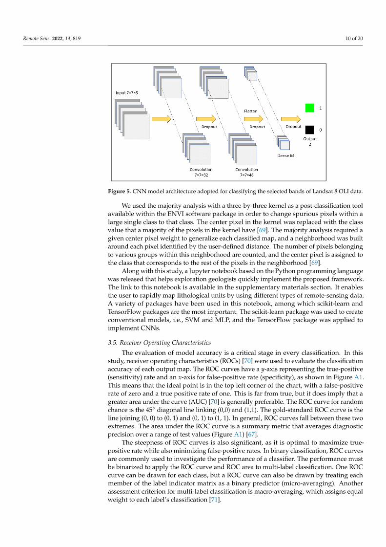
As shown in Figure 5, our CNN model uses two convolution layers with a kernelsize of 7 × 7, stride of 7, and fully linked layers. These layers are a network of seriallyconnected dense layers used for classification. In a fully connected network, every neuronfrom the first layer is connected to every neuron in the second layer. We examined otherkernel sizes and strides, and the best accuracy was achieved by the mentioned values.Model architectures are sensitive, and the same model architecture cannot be expected toprovide similar accuracy using different kernel sizes. Therefore, a few minor modificationsin the architecture are expected. We used the ReLU activation function for the input layersand the Softmax activation function in the final layer for classification in the CNN modelarchitecture. Furthermore, we used a root-mean-squared propagation optimizer with amaximum of 20 training epochs.

Remote Sens. 2022, 14, 819 10 of 20

Remote Sens. 2021, 13, x FOR PEER REVIEW 10 of 20

architecture are expected. We used the ReLU activation function for the input layers and the Softmax activation function in the final layer for classification in the CNN model ar-chitecture. Furthermore, we used a root-mean-squared propagation optimizer with a maximum of 20 training epochs.

Figure 5. CNN model architecture adopted for classifying the selected bands of Landsat 8 OLI data.

We used the majority analysis with a three-by-three kernel as a post-classification tool available within the ENVI software package in order to change spurious pixels within a large single class to that class. The center pixel in the kernel was replaced with the class value that a majority of the pixels in the kernel have [69]. The majority analysis required a given center pixel weight to generalize each classified map, and a neighborhood was built around each pixel identified by the user-defined distance. The number of pixels be-longing to various groups within this neighborhood are counted, and the center pixel is assigned to the class that corresponds to the rest of the pixels in the neighborhood [69].

Along with this study, a Jupyter notebook based on the Python programming lan-guage was released that helps exploration geologists quickly implement the proposed framework. The link to this notebook is available in the supplementary materials section. It enables the user to rapidly map lithological units by using different types of remote-sensing data. A variety of packages have been used in this notebook, among which scikit-learn and TensorFlow packages are the most important. The scikit-learn package was used to create conventional models, i.e., SVM and MLP, and the TensorFlow package was ap-plied to implement CNNs.

3.5. Receiver Operating Characteristics The evaluation of model accuracy is a critical stage in every classification. In this

study, receiver operating characteristics (ROCs) [70] were used to evaluate the classifica-tion accuracy of each output map. The ROC curves have a y-axis representing the true-positive (sensitivity) rate and an x-axis for false-positive rate (specificity), as shown in Fig-ure A1. This means that the ideal point is in the top left corner of the chart, with a false-positive rate of zero and a true positive rate of one. This is far from true, but it does imply that a greater area under the curve (AUC) [70] is generally preferable. The ROC curve for random chance is the 45° diagonal line linking (0,0) and (1,1). The gold-standard ROC curve is the line joining (0, 0) to (0, 1) and (0, 1) to (1, 1). In general, ROC curves fall be-tween these two extremes. The area under the ROC curve is a summary metric that aver-ages diagnostic precision over a range of test values (Figure A1) [67].

The steepness of ROC curves is also significant, as it is optimal to maximize true-positive rate while also minimizing false-positive rates. In binary classification, ROC

Figure 5. CNN model architecture adopted for classifying the selected bands of Landsat 8 OLI data.

We used the majority analysis with a three-by-three kernel as a post-classification toolavailable within the ENVI software package in order to change spurious pixels within alarge single class to that class. The center pixel in the kernel was replaced with the classvalue that a majority of the pixels in the kernel have [69]. The majority analysis required agiven center pixel weight to generalize each classified map, and a neighborhood was builtaround each pixel identified by the user-defined distance. The number of pixels belongingto various groups within this neighborhood are counted, and the center pixel is assigned tothe class that corresponds to the rest of the pixels in the neighborhood [69].

Along with this study, a Jupyter notebook based on the Python programming languagewas released that helps exploration geologists quickly implement the proposed framework.The link to this notebook is available in the supplementary materials section. It enablesthe user to rapidly map lithological units by using different types of remote-sensing data.A variety of packages have been used in this notebook, among which scikit-learn andTensorFlow packages are the most important. The scikit-learn package was used to createconventional models, i.e., SVM and MLP, and the TensorFlow package was applied toimplement CNNs.

3.5. Receiver Operating Characteristics

The evaluation of model accuracy is a critical stage in every classification. In thisstudy, receiver operating characteristics (ROCs) [70] were used to evaluate the classificationaccuracy of each output map. The ROC curves have a y-axis representing the true-positive(sensitivity) rate and an x-axis for false-positive rate (specificity), as shown in Figure A1.This means that the ideal point is in the top left corner of the chart, with a false-positiverate of zero and a true positive rate of one. This is far from true, but it does imply that agreater area under the curve (AUC) [70] is generally preferable. The ROC curve for randomchance is the 45◦ diagonal line linking (0,0) and (1,1). The gold-standard ROC curve is theline joining (0, 0) to (0, 1) and (0, 1) to (1, 1). In general, ROC curves fall between these twoextremes. The area under the ROC curve is a summary metric that averages diagnosticprecision over a range of test values (Figure A1) [67].

The steepness of ROC curves is also significant, as it is optimal to maximize true-positive rate while also minimizing false-positive rates. In binary classification, ROC curvesare commonly used to investigate the performance of a classifier. The performance mustbe binarized to apply the ROC curve and ROC area to multi-label classification. One ROCcurve can be drawn for each class, but a ROC curve can also be drawn by treating eachmember of the label indicator matrix as a binary predictor (micro-averaging). Anotherassessment criterion for multi-label classification is macro-averaging, which assigns equalweight to each label’s classification [71].

Remote Sens. 2022, 14, 819 11 of 20

4. Results4.1. Classified Lithological Maps

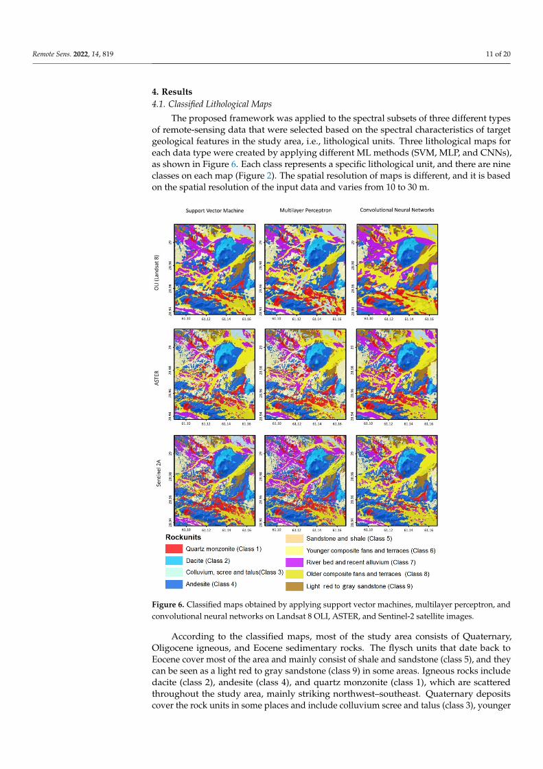
The proposed framework was applied to the spectral subsets of three different typesof remote-sensing data that were selected based on the spectral characteristics of targetgeological features in the study area, i.e., lithological units. Three lithological maps foreach data type were created by applying different ML methods (SVM, MLP, and CNNs),as shown in Figure 6. Each class represents a specific lithological unit, and there are nineclasses on each map (Figure 2). The spatial resolution of maps is different, and it is basedon the spatial resolution of the input data and varies from 10 to 30 m.

Remote Sens. 2021, 13, x FOR PEER REVIEW 11 of 20

curves are commonly used to investigate the performance of a classifier. The performance must be binarized to apply the ROC curve and ROC area to multi-label classification. One ROC curve can be drawn for each class, but a ROC curve can also be drawn by treating each member of the label indicator matrix as a binary predictor (micro-averaging). An-other assessment criterion for multi-label classification is macro-averaging, which assigns equal weight to each label’s classification [71].

4. Results 4.1. Classified Lithological Maps

The proposed framework was applied to the spectral subsets of three different types of remote-sensing data that were selected based on the spectral characteristics of target geological features in the study area, i.e., lithological units. Three lithological maps for each data type were created by applying different ML methods (SVM, MLP, and CNNs), as shown in Figure 6. Each class represents a specific lithological unit, and there are nine classes on each map (Figure 2). The spatial resolution of maps is different, and it is based on the spatial resolution of the input data and varies from 10 to 30 m.

Figure 6. Classified maps obtained by applying support vector machines, multilayer perceptron, andconvolutional neural networks on Landsat 8 OLI, ASTER, and Sentinel-2 satellite images.

According to the classified maps, most of the study area consists of Quaternary,Oligocene igneous, and Eocene sedimentary rocks. The flysch units that date back toEocene cover most of the area and mainly consist of shale and sandstone (class 5), and theycan be seen as a light red to gray sandstone (class 9) in some areas. Igneous rocks includedacite (class 2), andesite (class 4), and quartz monzonite (class 1), which are scatteredthroughout the study area, mainly striking northwest–southeast. Quaternary depositscover the rock units in some places and include colluvium scree and talus (class 3), younger

Remote Sens. 2022, 14, 819 12 of 20

composite alluvial fans and terraces (class 6), older composite alluvial fans and terraces(class 8), and riverbed and recent alluvium (class 7).

4.2. Accuracy Assessment and Validation

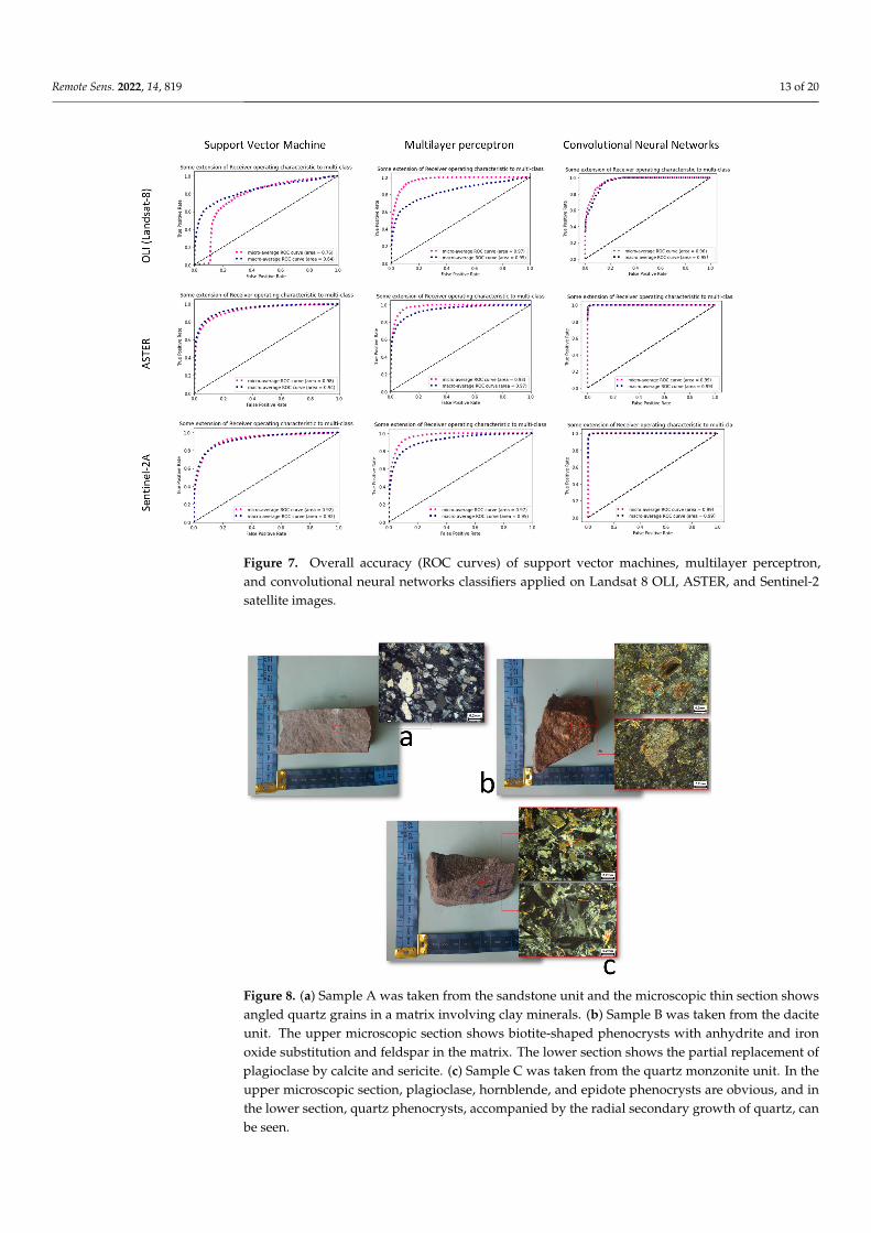
Table 1 depicts the accuracy of each class, and Figure 7 demonstrates the micro andmacro average ROC curve for all nine classified maps. According to the ROC curves shownin Figure 7, the lithological units were classified more accurately by using the combinationof CNN and ASTER data. However, the result is almost the same as Sentinel-2 data. TheAUC of micro and macro averages is close to one in these plots. Considering the AUCs, theMLP outperforms the SVM, and it is ranked second in terms of accuracy. On the other hand,after the ASTER data, the Sentinel-2 data yielded the most accurate results for lithologicalmapping in the study area, and the OLI is ranked last, which could be anticipated. Thecombination of SVM and OLI shows the lowest accuracy, where the micro average is 0.76,and the macro average is 0.84.

Table 1. Accuracy (AUC) of each class (lithological unit) obtained by applying SVM, MLP, and CNNon Landsat 8 OLI, ASTER, and Sentinel-2 remote sensing data.

Landsat 8 OLI ASTER Sentinel-2

Lithology Type ClassNumber SVM MLP CNN SVM MLP CNN SVM MLP CNN

Quartz monzonite 1 0.98 0.98 1 0.97 0.99 1 0.88 0.98 0.99Dacite 2 0.99 0.99 0.99 0.88 0.99 1 0.89 0.99 0.99

Colluvium screeand talus 3 0.97 0.97 0.99 1.00 0.99 0.99 0.99 0.99 0.99

Andesite 4 0.91 0.91 0.99 0.90 0.95 0.99 0.80 0.91 0.97Sandstone and

shale 5 0.97 0.97 0.99 0.89 0.97 1 0.94 0.96 0.98

Youngercomposite alluvialfans and terraces

6 0.92 0.92 0.99 0.94 0.94 0.99 0.95 0.94 0.99

River bed andrecent alluvium 7 0.95 0.95 0.99 0.96 0.99 1 0.92 0.92 0.99

Older compositealluvial fans and

terraces8 0.90 0.90 1 0.95 0.90 0.99 0.95 0.91 0.99

Light red to graysandstone 9 0.95 0.95 0.99 0.97 0.98 1 0.96 0.94 0.99

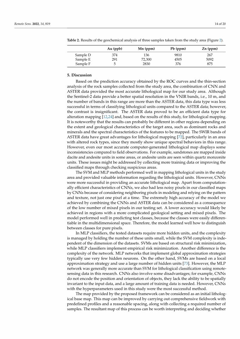
In addition to the ROC curves, several rock samples were collected from the study areato validate the lithological maps, particularly in places with little ground-truth data. Thesesamples were mostly collected from the places where rock types are classified as quartzmonzonite, andesite, dacite, and sandstone, and three of them, along with their polishedthin sections, are shown in Figure 8. The sampling locations are shown in Figure 1 andlabeled as A–C. The results obtained by investigating the polished thin sections indicate thatthe classifiers have been successful in the sampling regions. Moreover, we analyzed threesamples from the study area, as shown in Figure 1, labeled as D–F, using the inductivelycoupled plasma–mass spectrometry (ICP–MS) for determining the concentration values ofgold, manganese, lead, and zinc. Based on the laboratory analysis, the margins of igneousunits in the study area are of great importance in terms of economic mineralization, andthe geochemical analyses confirm this observation (Table 2).

Remote Sens. 2022, 14, 819 13 of 20

Remote Sens. 2021, 13, x FOR PEER REVIEW 12 of 20

Figure 6. Classified maps obtained by applying support vector machines, multilayer perceptron, and convolutional neural networks on Landsat 8 OLI, ASTER, and Sentinel-2 satellite images.

According to the classified maps, most of the study area consists of Quaternary, Oli-gocene igneous, and Eocene sedimentary rocks. The flysch units that date back to Eocene cover most of the area and mainly consist of shale and sandstone (class 5), and they can be seen as a light red to gray sandstone (class 9) in some areas. Igneous rocks include dacite (class 2), andesite (class 4), and quartz monzonite (class 1), which are scattered throughout the study area, mainly striking northwest–southeast. Quaternary deposits cover the rock units in some places and include colluvium scree and talus (class 3), younger composite alluvial fans and terraces (class 6), older composite alluvial fans and terraces (class 8), and riverbed and recent alluvium (class 7).

4.2. Accuracy Assessment and Validation Table 1 depicts the accuracy of each class, and Figure 7 demonstrates the micro and

macro average ROC curve for all nine classified maps. According to the ROC curves shown in Figure 7, the lithological units were classified more accurately by using the com-bination of CNN and ASTER data. However, the result is almost the same as Sentinel-2 data. The AUC of micro and macro averages is close to one in these plots. Considering the AUCs, the MLP outperforms the SVM, and it is ranked second in terms of accuracy. On the other hand, after the ASTER data, the Sentinel-2 data yielded the most accurate results for lithological mapping in the study area, and the OLI is ranked last, which could be anticipated. The combination of SVM and OLI shows the lowest accuracy, where the mi-cro average is 0.76, and the macro average is 0.84.

Figure 7. Overall accuracy (ROC curves) of support vector machines, multilayer perceptron,and convolutional neural networks classifiers applied on Landsat 8 OLI, ASTER, and Sentinel-2satellite images.Remote Sens. 2021, 13, x FOR PEER REVIEW 14 of 20

Figure 8. (a) Sample A was taken from the sandstone unit and the microscopic thin section shows angled quartz grains in a matrix involving clay minerals. (b) Sample B was taken from the dacite unit. The upper microscopic section shows biotite-shaped phenocrysts with anhydrite and iron ox-ide substitution and feldspar in the matrix. The lower section shows the partial replacement of pla-gioclase by calcite and sericite. (c) Sample C was taken from the quartz monzonite unit. In the upper microscopic section, plagioclase, hornblende, and epidote phenocrysts are obvious, and in the lower section, quartz phenocrysts, accompanied by the radial secondary growth of quartz, can be seen.

5. Discussion Based on the prediction accuracy obtained by the ROC curves and the thin-section

analysis of the rock samples collected from the study area, the combination of CNN and ASTER data provided the most accurate lithological map for our study area. Although the Sentinel-2 data provide a better spatial resolution in the VNIR bands, i.e., 10 m, and the number of bands in this range are more than the ASTER data, this data type was less successful in terms of classifying lithological units compared to the ASTER data; however, the contrast is insignificant. The ASTER data proved to be an efficient data type for alter-ation mapping [12,24] and, based on the results of this study, for lithological mapping. It is noteworthy that the results can probably be different in other regions depending on the extent and geological characteristics of the target area, such as dominant rocks and min-erals and the spectral characteristics of the features to be mapped. The SWIR bands of ASTER data have great advantages for lithological mapping [72], particularly in an area with altered rock types, since they mostly show unique spectral behaviors in this range. However, even our most accurate computer-generated lithological map displays some in-consistencies compared to field observations. For example, sandstones are mapped inside dacite and andesite units in some areas, or andesite units are seen within quartz monzo-nite units. These issues might be addressed by collecting more training data or improving the classified maps through checking suspicious areas.

Figure 8. (a) Sample A was taken from the sandstone unit and the microscopic thin section showsangled quartz grains in a matrix involving clay minerals. (b) Sample B was taken from the daciteunit. The upper microscopic section shows biotite-shaped phenocrysts with anhydrite and ironoxide substitution and feldspar in the matrix. The lower section shows the partial replacement ofplagioclase by calcite and sericite. (c) Sample C was taken from the quartz monzonite unit. In theupper microscopic section, plagioclase, hornblende, and epidote phenocrysts are obvious, and inthe lower section, quartz phenocrysts, accompanied by the radial secondary growth of quartz, canbe seen.

Remote Sens. 2022, 14, 819 14 of 20

Table 2. Results of the geochemical analysis of three samples taken from the study area (Figure 2).

Au (ppb) Mn (ppm) Pb (ppm) Zn (ppm)

Sample D 374 136 9810 267Sample E 291 72,300 4505 5092Sample F 5 2830 376 875

5. Discussion

Based on the prediction accuracy obtained by the ROC curves and the thin-sectionanalysis of the rock samples collected from the study area, the combination of CNN andASTER data provided the most accurate lithological map for our study area. Althoughthe Sentinel-2 data provide a better spatial resolution in the VNIR bands, i.e., 10 m, andthe number of bands in this range are more than the ASTER data, this data type was lesssuccessful in terms of classifying lithological units compared to the ASTER data; however,the contrast is insignificant. The ASTER data proved to be an efficient data type foralteration mapping [12,24] and, based on the results of this study, for lithological mapping.It is noteworthy that the results can probably be different in other regions depending onthe extent and geological characteristics of the target area, such as dominant rocks andminerals and the spectral characteristics of the features to be mapped. The SWIR bands ofASTER data have great advantages for lithological mapping [72], particularly in an areawith altered rock types, since they mostly show unique spectral behaviors in this range.However, even our most accurate computer-generated lithological map displays someinconsistencies compared to field observations. For example, sandstones are mapped insidedacite and andesite units in some areas, or andesite units are seen within quartz monzoniteunits. These issues might be addressed by collecting more training data or improving theclassified maps through checking suspicious areas.

The SVM and MLP methods performed well in mapping lithological units in the studyarea and provided valuable information regarding the lithological units. However, CNNswere more successful in providing an accurate lithological map. Apart from computation-ally efficient characteristics of CNNs, we also had less noisy pixels in our classified mapsby CNNs because of considering neighboring pixels in modeling and relying on the patternand texture, not just one pixel at a time. The extremely high accuracy of the model weachieved by combining the CNNs and ASTER data can be considered as a consequenceof the low number of mixed pixels in our testing set. A lower accuracy would likely beachieved in regions with a more complicated geological setting and mixed pixels. Themodel performed well in predicting test classes, because the classes were easily differen-tiable in the multidimensional space. Therefore, the model learned well how to distinguishbetween classes for pure pixels.

In MLP classifiers, the tested datasets require more hidden units, and the complexityis managed by holding the number of these units small, while the SVM complexity is inde-pendent of the dimension of the datasets. SVMs are based on structural risk minimization,while MLP classifiers implement empirical risk minimization. Another difference is thecomplexity of the network. MLP networks that implement global approximation strategiestypically use very few hidden neurons. On the other hand, SVMs are based on a localapproximation strategy and use a large number of hidden units [73]. However, the MLPnetwork was generally more accurate than SVM for lithological classification using remote-sensing data in this research. CNNs also involve some disadvantages; for example, CNNsdo not encode the position and orientation of objects, they lack the ability to be spatiallyinvariant to the input data, and a large amount of training data is needed. However, CNNswith the hyperparameters used in this study were the most successful method.

The map provided by the proposed framework can be considered as an initial litholog-ical base map. This map can be improved by carrying out comprehensive fieldwork withpredefined profiles and a reasonable spacing, along with collecting a required number ofsamples. The resultant map of this process can be worth interpreting and deciding whether

Remote Sens. 2022, 14, 819 15 of 20

to continue the exploration operation in a region. According to the laboratory analysis andfield observations, gold, manganese, lead, and zinc mineralizations and the interaction ofpyrite with manganese-impregnated siliceous veins have been found in the margins ofigneous units and mapped accurately in the lithological maps. In addition, the geochemicalanalysis of the samples collected from potential locations supports the high probability ofeconomic gold mineralization in the study area.

ML methods have been widely used in remote-sensing-data analysis, but there arestill gaps in predictive uncertainty quantification. In general, it is difficult to assess theuncertainty of remote-sensing model applications. Model validation is usually performedby comparing it with ground truth or alternative information believed to represent groundtruth. Different approaches have been developed to address validation issues, and differentmodels are possible. Bayesian inference provides a principled approach for quantifying theuncertainty of model parameters. Recently, there have been major advances in Bayesianneural networks and Bayesian deep learning. However, these methods have not beenmuch used for remote sensing, and their application for geological exploration is absent.In future studies, we are planning to use other deep learning methods to map geologicalfeatures [34], such as Bayesian neural networks, since it provides principled uncertaintyquantification via the posterior distribution [74]. These methods may provide a meaningfulinterpretation of remote-sensing data in the face of challenges, such as data noise, sparsedatasets, and missing data. Uncertainty quantification using Bayesian inference can beused to predict the uncertainty associated with model parameters and data. As a result,applying these methods can play an essential role in the evolution of geological remotesensing and improve its efficiency in mineral exploration.

6. Conclusions

Nowadays, geoscientists are equipped with the latest groundbreaking and efficient MLmethods to work with big data, such as remote-sensing data. In this study, three different MLmethods were used to process three types of remote-sensing data by mapping lithological unitsof a region in the southeast of Iran. We classified the remote-sensing data and discriminatedlithological units, providing valuable information for mineral exploration. We showed theefficiency of applying machine- and deep-learning techniques on remote-sensing data andobserved that the CNN and ASTER data combination provides the most accurate lithologicalmap of the study area based on the ROC curves, and the test data were successfully predicted.Such maps can be considered base maps for further geological fieldworks and a reliable factoraiding in deciding for mineral-exploration operations.

We addressed the challenges of mapping lithological units on the ground and proposeda framework to overcome them. Our framework presented in a Jupyter notebook is an open-source community tool for mapping lithological units by using multi- or hyperspectraldata. This notebook can significantly enhance the ability of exploration geologists tomap lithological units. It can be considered a fast, reliable, and low-cost approach forgenerating a remote-sensing evidential layer and delineating favorable loci for preciousmineral deposits at any stage of an exploration program. The framework can be improvedby optimizing SVM, MLP, and CNN hyperparameters. Moreover, other ML methods, suchas random forest, naive Bayes, k-nearest neighbors, and minimum distance, can be addedto this framework to compare their efficiency with other methods.

Supplementary Materials: The Jupyter notebook and datasets used in this study are available athttps://github.com/sydney-machine-learning/deeplearning_lithology (accessed on 20 November 2021).

Author Contributions: H.S. and E.F. made an equal contribution to this study. Conceptualization,H.S., E.F. and R.C.; methodology, H.S., E.F. and R.C.; software, H.S., E.F. and R.C.; validation, H.S.and E.F.; writing—original draft preparation, H.S., E.F., E.H. and R.C.; writing—review and editing,A.B.P., B.P. and D.M.; visualization, H.S. and E.F.; supervision, R.C. All authors have read and agreedto the published version of the manuscript.

Funding: This research was supported by the Australian Research Council (Grant No.: LP210100173).

Remote Sens. 2022, 14, 819 16 of 20

Data Availability Statement: The datasets used in this study, including remote sensing and groundtruth data, are available at https://github.com/sydney-machine-learning/deeplearning_lithology(accessed on 20 November 2021).

Acknowledgments: The authors would like to thank L. S. Galvao for handling this paper andanonymous reviewers for providing constructive comments that improved the manuscript.

Conflicts of Interest: The authors declare no conflict of interest.

Appendix A

Table A1. Technical performance and attributes of Landsat 8, Sentinel-2, and ASTER data [46–48].

Satellite/Sensor Subsystem Band Number Spectral Range(Micrometers)

GroundResolution (m)

Swath Width(Km)

Year ofLaunch

Landsat 8

OLI

Band 1 Coastal Aerosol 0.43–0.45 30

185 2013

Band 2 Blue 0.45–0.51 30Band 3 Green 0.53–0.59 30Band 4 Red 0.64–0.67 30

Band 5 Near Infrared (NIR) 0.85–0.88 30Band 6 SWIR 1 1.57–1.65 30Band 7 SWIR 2 2.11–2.29 30

Band 8 Panchromatic 0.50–0.68 15Band 9 Cirrus 1.36–1.38 30

TIR

Band 10 Thermal Infrared(TIRS 1) 10.60–11.19 100

Band 11 Thermal Infrared(TIRS 2) 11.50–12.51 100

ASTER

VNIRBand 1 0.520–0.600 15

60 1999

Band 2 0.630–0.690 15Band 3 0.780–0.860 15

SWIR

Band 4 1.600–1.700 30Band 5 2.145–2.185 30Band 6 2.185–2.225 30Band 7 2.235–2.285 30Band 8 2.295–2.365 30Band 9 2.360–2.430 30

TIR

Band 10 8.125–8.475 90Band 11 8.475–8.825 90Band 12 8.925–9.275Band 13 10.250–10.950Band 14 10.950–11.650

Sentinel-2

Band 1 Coastal Aerosol 0.433–0.453 60

290 2015

Band 2 Blue 0.458–0.523 10Band 3 Green 0.543–0.578 10Band 4 Red 0.650–0.680 10

Band 5 Red Edge 1 0.698–0.713 20Band 6 Red Edge 2 0.733–0.748 20Band 7 Red Edge 3 0.773–0.793 20

Band 8 NIR 0.785–0.900 10Band 8A Narrow NIR 0.855–0.875 20Band 9 Water-Vapor 0.935–0.955 60

Band 10 SWIR/Cirrus 1.360–1.390 60Band 11 SWIR 1 1.565–1.655 20Band 12 SWIR 2 2.100–2.280 20

Remote Sens. 2022, 14, 819 17 of 20

Remote Sens. 2021, 13, x FOR PEER REVIEW 17 of 20

Band 7 SWIR 2 2.11–2.29 30 Band 8 Panchromatic 0.50–0.68 15

Band 9 Cirrus 1.36–1.38 30

TIR

Band 10 Thermal Infrared (TIRS 1)

10.60–11.19 100

Band 11 Thermal Infrared (TIRS 2)

11.50–12.51 100

ASTER

VNIR Band 1 0.520–0.600 15

60 1999

Band 2 0.630–0.690 15 Band 3 0.780–0.860 15

SWIR

Band 4 1.600–1.700 30 Band 5 2.145–2.185 30 Band 6 2.185–2.225 30 Band 7 2.235–2.285 30 Band 8 2.295–2.365 30 Band 9 2.360–2.430 30

TIR

Band 10 8.125–8.475 90 Band 11 8.475–8.825 90 Band 12 8.925–9.275 Band 13 10.250–10.950 Band 14 10.950–11.650

Sentinel-2

Band 1 Coastal Aerosol 0.433–0.453 60

290 2015

Band 2 Blue 0.458–0.523 10 Band 3 Green 0.543–0.578 10 Band 4 Red 0.650–0.680 10

Band 5 Red Edge 1 0.698–0.713 20 Band 6 Red Edge 2 0.733–0.748 20 Band 7 Red Edge 3 0.773–0.793 20

Band 8 NIR 0.785–0.900 10 Band 8A Narrow NIR 0.855–0.875 20 Band 9 Water-Vapor 0.935–0.955 60 Band 10 SWIR/Cirrus 1.360–1.390 60

Band 11 SWIR 1 1.565–1.655 20 Band 12 SWIR 2 2.100–2.280 20

Figure A1. Three imaginary ROC curves reflecting the gold standard’s diagnostic precision (lines A;AUC = 1) on the upper and left axes in the unit square, a normal ROC curve (curve B; AUC = 0.85),and a diagonal line leading to random chance (line C; AUC = 0.5) are shown. The ROC curve shiftstoward A as the diagnostic-test precision increases and the AUC reaches 1 [75].

References1. Othman, A.; Gloaguen, R. Improving lithological mapping by SVM classification of spectral and morphological features: The

discovery of a new chromite body in the Mawat ophiolite complex (Kurdistan, NE Iraq). Remote Sens. 2014, 6, 6867–6896.[CrossRef]

2. Qing, F.; Zhao, Y.; Meng, X.; Su, X.; Qi, T.; Yue, D. Application of machine learning to debris flow susceptibility mapping alongthe China–Pakistan Karakoram highway. Remote Sens. 2020, 12, 2933. [CrossRef]

3. Torabi, A.; Berg, S.S. Scaling of fault attributes: A review. Mar. Pet. Geol. 2011, 28, 1444–1460. [CrossRef]4. Ding, W.-C.; Li, T.-D.; Chen, X.-H.; Chen, J.-P.; Xu, S.-L.; Zhang, Y.-P.; Li, B.; Yang, Q. Intra-continental deformation and tectonic

evolution of the West Junggar Orogenic Belt, Central Asia: Evidence from remote sensing and structural geological analyses.Geosci. Front. 2020, 11, 651–663. [CrossRef]

5. Liu, L.; Zhou, J.; Jiang, D.; Zhuang, D.; Mansaray, L.R.; Zhang, B. Targeting mineral resources with remote sensing and field datain the Xiemisitai area, West Junggar, Xinjiang, China. Remote Sens. 2013, 5, 3156–3171. [CrossRef]

6. Radford, D.D.G.; Cracknell, M.J.; Roach, M.J.; Cumming, G. V Geological mapping in Western Tasmania using radar and randomforests. IEEE J. Sel. Top. Appl. Earth Obs. Remote Sens. 2018, 11, 3075–3087. [CrossRef]

7. Shirmard, H.; Farahbakhsh, E.; Müller, R.D.; Chandra, R. A review of machine learning in processing remote sensing data formineral exploration. Remote Sens. Environ. 2022, 268, 112750. [CrossRef]

8. Brimhall, G.H.; Dilles, J.H.; Proffett, J.M. The Role of Geologic Mapping in Mineral Exploration. Wealth Creat. Miner. Ind. Integr.Sci. Business Educ. 2005, 12, 221–241.

9. Rowan, L.C.; Schmidt, R.G.; Mars, J.C. Distribution of hydrothermally altered rocks in the Reko Diq, Pakistan mineralized areabased on spectral analysis of ASTER data. Remote Sens. Environ. 2006, 104, 74–87. [CrossRef]

10. Latifovic, R.; Pouliot, D.; Campbell, J. Assessment of convolution neural networks for surficial geology mapping in the South Raegeological region, Northwest Territories, Canada. Remote Sens. 2018, 10, 307. [CrossRef]

11. Asadzadeh, S.; de Souza Filho, C.R. A review on spectral processing methods for geological remote sensing. Int. J. Appl. EarthObs. Geoinf. 2016, 47, 69–90. [CrossRef]

12. Rezaei, A.; Hassani, H.; Moarefvand, P.; Golmohammadi, A. Lithological mapping in Sangan region in Northeast Iran usingASTER satellite data and image processing methods. Geol. Ecol. Landsc. 2020, 4, 59–70. [CrossRef]

13. Lazecký, M.; Spaans, K.; González, P.J.; Maghsoudi, Y.; Morishita, Y.; Albino, F.; Elliott, J.; Greenall, N.; Hatton, E.; Hooper, A.; et al.LiCSAR: An automatic InSAR tool for measuring and monitoring tectonic and volcanic activity. Remote Sens. 2020, 12, 2430.[CrossRef]

14. Beiranvand Pour, A.; Hashim, M. ASTER, ALI and Hyperion sensors data for lithological mapping and ore minerals exploration.Springerplus 2014, 3, 130. [CrossRef] [PubMed]

15. Shirmard, H.; Farahbakhsh, E.; Beiranvand Pour, A.; Muslim, A.M.; Müller, R.D.; Chandra, R. Integration of selective dimension-ality reduction techniques for mineral exploration using ASTER satellite data. Remote Sens. 2020, 12, 1261. [CrossRef]

Remote Sens. 2022, 14, 819 18 of 20

16. van der Meer, F.D.; van der Werff, H.M.A.; van Ruitenbeek, F.J.A.; Hecker, C.A.; Bakker, W.H.; Noomen, M.F.; van der Meijde, M.;Carranza, E.J.M.; de Smeth, J.B.; Woldai, T. Multi- and hyperspectral geologic remote sensing: A review. Int. J. Appl. Earth Obs.Geoinf. 2012, 14, 112–128. [CrossRef]

17. Kuhn, S.; Cracknell, M.J.; Reading, A.M. Lithologic mapping using Random Forests applied to geophysical and remote-sensingdata: A demonstration study from the Eastern Goldfields of Australia. Geophysics 2018, 83, B183–B193. [CrossRef]

18. Farahbakhsh, E.; Chandra, R.; Olierook, H.; Scalzo, R.; Clark, C.; Reddy, S.; Müller, D. Computer vision-based framework forextracting tectonic lineaments from optical remote sensing data. Int. J. Remote Sens. 2020, 41, 1760–1787. [CrossRef]

19. Sun, T.; Chen, F.; Zhong, L.; Liu, W.; Wang, Y. GIS-based mineral prospectivity mapping using machine learning methods: A casestudy from Tongling ore district, eastern China. Ore Geol. Rev. 2019, 109, 26–49. [CrossRef]

20. Cracknell, M.J.; Reading, A.M. Geological mapping using remote sensing data: A comparison of five machine learning algorithms,their response to variations in the spatial distribution of training data and the use of explicit spatial information. Comput. Geosci.2014, 63, 22–33. [CrossRef]

21. Kanevski, M. Machine Learning for Spatial Environmental Data; EPFL Press: New York, NY, USA, 2009.22. Ye, B.; Tian, S.; Ge, J.; Sun, Y. Assessment of WorldView-3 data for lithological mapping. Remote Sens. 2017, 9, 1132. [CrossRef]23. Farahbakhsh, E.; Shirmard, H.; Bahroudi, A.; Eslamkish, T. Fusing ASTER and QuickBird-2 satellite data for detailed investigation

of porphyry copper deposits using PCA; Case study of Naysian deposit, Iran. J. Indian Soc. Remote Sens. 2016, 44, 525–537.[CrossRef]

24. Beiranvand Pour, A.; Hashim, M.; Hong, J.K.; Park, Y. Lithological and alteration mineral mapping in poorly exposed lithologiesusing Landsat-8 and ASTER satellite data: North-eastern Graham Land, Antarctic Peninsula. Ore Geol. Rev. 2019, 108, 112–133.[CrossRef]

25. Sekandari, M.; Masoumi, I.; Beiranvand Pour, A.; Muslim, A.M.; Rahmani, O.; Hashim, M.; Zoheir, B.; Pradhan, B.; Misra, A.;Aminpour, S.M. Application of Landsat-8, Sentinel-2, ASTER and WorldView-3 spectral imagery for exploration of carbonate-hosted Pb-Zn deposits in the Central Iranian Terrane (CIT). Remote Sens. 2020, 12, 1239. [CrossRef]

26. Yu, L.; Porwal, A.; Holden, E.-J.; Dentith, M.C. Towards automatic lithological classification from remote sensing data usingsupport vector machines. Comput. Geosci. 2012, 45, 229–239. [CrossRef]

27. Bressan, T.S.; Kehl de Souza, M.; Girelli, T.J.; Junior, F.C. Evaluation of machine learning methods for lithology classification usinggeophysical data. Comput. Geosci. 2020, 139, 104475. [CrossRef]

28. Bachri, I.; Hakdaoui, M.; Raji, M.; Teodoro, A.C.; Benbouziane, A. Machine learning algorithms for automatic lithological mappingusing remote sensing data: A case study from Souk Arbaa Sahel, Sidi Ifni Inlier, Western Anti-Atlas, Morocco. ISPRS Int. J.Geo-Inf. 2019, 8, 248. [CrossRef]

29. Atangana Otele, C.G.; Onabid, M.A.; Assembe, P.S.; Nkenlifack, M. Updated lithological map in the Forest zone of the Centre,South and East regions of Cameroon using multilayer perceptron neural network and Landsat images. J. Geosci. Environ. Prot.2021, 9, 120–134. [CrossRef]

30. Venkatesh, Y.V.; Kumar Raja, S. On the classification of multispectral satellite images using the multilayer perceptron. PatternRecognit. 2003, 36, 2161–2175. [CrossRef]

31. Sergi, R.; Solaiman, B.; Mouchot, M.-C.; Pasquariello, G.; Pósa, P. Landsat-TM image classification using principal componentsanalysis and neural networks. In Proceedings of the International Geoscience and Remote Sensing Symposium: QuantitativeRemote Sensing for Science and Applications, Firenze, Italy, 10–14 July 1995; Volume 3, pp. 1927–1929.

32. Neupane, B.; Horanont, T.; Aryal, J. Deep learning-based semantic segmentation of urban features in satellite images: A reviewand meta-analysis. Remote Sens. 2021, 13, 808. [CrossRef]

33. He, Z.; Liu, H.; Wang, Y.; Hu, J. Generative adversarial networks-based semi-supervised learning for hyperspectral imageclassification. Remote Sens. 2017, 9, 1042. [CrossRef]

34. Sang, X.; Xue, L.; Ran, X.; Li, X.; Liu, J.; Liu, Z. Intelligent high-resolution geological mapping based on SLIC-CNN. ISPRS Int. J.Geo-Inf. 2020, 9, 99. [CrossRef]

35. Chen, Y.-Y.; Lin, Y.-H.; Kung, C.-C.; Chung, M.-H.; Yen, I.-H. Design and implementation of cloud analytics-assisted smart powermeters considering advanced artificial intelligence as edge analytics in demand-side management for smart homes. Sensors 2019,19, 2047. [CrossRef] [PubMed]

36. Georgiou, T.; Liu, Y.; Chen, W.; Lew, M. A survey of traditional and deep learning-based feature descriptors for high dimensionaldata in computer vision. Int. J. Multimed. Inf. Retr. 2020, 9, 135–170. [CrossRef]

37. Shambhu, S.; Koundal, D.; Das, P.; Sharma, C. Binary classification of COVID-19 CT images using CNN: COVID diagnosis usingCT. Int. J. E-Health Med. Commun. 2022, 13, 1–13. [CrossRef]

38. Yang, M.; Liu, Y.; You, Z. The Euclidean embedding learning based on convolutional neural network for stereo matching.Neurocomputing 2017, 267, 195–200. [CrossRef]

39. Jing, L.; Zhao, M.; Li, P.; Xu, X. A convolutional neural network based feature learning and fault diagnosis method for thecondition monitoring of gearbox. Measurement 2017, 111, 1–10. [CrossRef]

40. Ma, L.; Liu, Y.; Zhang, X.; Ye, Y.; Yin, G.; Johnson, B.A. Deep learning in remote sensing applications: A meta-analysis and review.ISPRS J. Photogramm. Remote Sens. 2019, 152, 166–177. [CrossRef]

41. Saliu, O.; Curilla, D.; Lennon, M.; Chung, A. Lessons learned: Deep learning for mineral exploration. In Proceedings of the FirstEAGE Conference on Machine Learning in Americas, Online, 22–24 September 2020.

Remote Sens. 2022, 14, 819 19 of 20

42. Mei, S.; Geng, Y.; Hou, J.; Du, Q. Learning hyperspectral images from RGB images via a coarse-to-fine CNN. Sci. China Inf. Sci.2022, 65, 152102. [CrossRef]

43. Litjens, G.; Kooi, T.; Bejnordi, B.E.; Setio, A.A.A.; Ciompi, F.; Ghafoorian, M.; van der Laak, J.A.W.M.; van Ginneken, B.; Sánchez,C.I. A survey on deep learning in medical image analysis. Med. Image Anal. 2017, 42, 60–88. [CrossRef]

44. Parsolang Engineering Consultant Company. Map Report: Deh Reza Exploration Area, Sistan and Baluchestan Province; ParsolangEngineering Consultant Company: Tehran, Iran, 2021.

45. Groves, D.I.; Santosh, M.; Zhang, L. A scale-integrated exploration model for orogenic gold deposits based on a mineral systemapproach. Geosci. Front. 2020, 11, 719–738. [CrossRef]

46. Vaughn, I. Landsat 8 (L8) Data Users Handbook; US Geological Survey: Sioux Falls, SD, USA, 2019.47. Abrams, M.; Hook, S.; Ramachandran, B. ASTER User Handbook; Jet Propulsion Laboratory: Pasadena, CA, USA, 2002.48. SUHET. Sentinel-2 User Handbook; European Space Agency: Paris, France, 2015.49. Grosse, R.; Johnson, M.K.; Adelson, E.H.; Freeman, W.T. Ground truth dataset and baseline evaluations for intrinsic image

algorithms. In Proceedings of the IEEE 12th International Conference on Computer Vision, Kyoto, Japan, 29 September–2 October2009; pp. 2335–2342.

50. Krig, S. Ground Truth Data, Content, Metrics, and Analysis. In Computer Vision Metrics; Springer: Berlin/Heidelberg, Germany,2014; pp. 283–311.

51. Maxwell, A.E.; Warner, T.A.; Fang, F. Implementation of machine-learning classification in remote sensing: An applied review.Int. J. Remote Sens. 2018, 39, 2784–2817. [CrossRef]

52. Gewali, U.B.; Monteiro, S.T.; Saber, E. Machine learning based hyperspectral image analysis: A survey. arXiv 2018,arXiv:1802.08701.

53. Liu, P.; Choo, K.-K.R.; Wang, L.; Huang, F. SVM or deep learning? A comparative study on remote sensing image classification.Soft Comput. 2017, 21, 7053–7065. [CrossRef]

54. Maepa, F.; Smith, R.S.; Tessema, A. Support vector machine and artificial neural network modelling of orogenic gold prospectivitymapping in the Swayze greenstone belt, Ontario, Canada. Ore Geol. Rev. 2021, 130, 103968. [CrossRef]

55. Abedi, M.; Norouzi, G.-H.; Bahroudi, A. Support vector machine for multi-classification of mineral prospectivity areas. Comput.Geosci. 2012, 46, 272–283. [CrossRef]

56. Pal, M.; Rasmussen, T.; Porwal, A. Optimized lithological mapping from multispectral and hyperspectral remote sensing imagesusing fused multi-classifiers. Remote Sens. 2020, 12, 177. [CrossRef]

57. Abdolmaleki, M.; Rasmussen, T.M.; Pal, M.K. Exploration of IOCG mineralizations using integration of space-borne remotesensing data with airborne geophysical data. ISPRSn Int. Arch. Photogramm. Remote Sens. Spat. Inf. Sci. 2020, XLIII-B3-2, 9–16.[CrossRef]

58. Cardoso-Fernandes, J.; Teodoro, A.C.; Lima, A.; Roda-Robles, E. Semi-Automatization of Support Vector Machines to MapLithium (Li) Bearing Pegmatites. Remote Sens. 2020, 12, 2319. [CrossRef]

59. Lek, S.; Guégan, J.F. Artificial neural networks as a tool in ecological modelling, an introduction. Ecol. Modell. 1999, 120, 65–73.[CrossRef]

60. Wang, G.; Yan, C.; Zhang, S.; Song, Y. Probabilistic neural networks and fractal method applied to mineral potential mapping inLuanchuan region, Henan Province, China. In Proceedings of the Sixth International Conference on Natural Computation, Yantai,China, 10–12 August 2010; pp. 1003–1007.

61. Subasi, A.; Erçelebi, E. Classification of EEG signals using neural network and logistic regression. Comput. Methods ProgramsBiomed. 2005, 78, 87–99. [CrossRef] [PubMed]

62. Lecun, Y.; Bottou, L.; Bengio, Y.; Haffner, P. Gradient-based learning applied to document recognition. Proc. IEEE 1998, 86,2278–2324. [CrossRef]

63. Li, H.; Li, X.; Yuan, F.; Jowitt, S.M.; Zhang, M.; Zhou, J.; Zhou, T.; Li, X.; Ge, C.; Wu, B. Convolutional neural network andtransfer learning based mineral prospectivity modeling for geochemical exploration of Au mineralization within the Guandian–Zhangbaling area, Anhui Province, China. Appl. Geochem. 2020, 122, 104747. [CrossRef]

64. Xin, M.; Wang, Y. Research on image classification model based on deep convolution neural network. EURASIP J. Image VideoProcess. 2019, 2019, 40. [CrossRef]

65. Shuo, H.; Kang, H. Deep CNN for Classification of Image Contents. In Proceedings of the 2021 3rd International Conference onImage Processing and Machine Vision (IPMV), Hong Kong, China, 22–24 May 2021; ACM: New York, NY, USA, 2021; pp. 60–65.

66. Newman, E.; Kilmer, M.; Horesh, L. Image classification using local tensor singular value decompositions. In Proceedings of theIEEE 7th International Workshop on Computational Advances in Multi-Sensor Adaptive Processing (CAMSAP), Curaçao, TheNetherlands, 10–13 December 2017; pp. 1–5.

67. Gu, J.; Wang, Z.; Kuen, J.; Ma, L.; Shahroudy, A.; Shuai, B.; Liu, T.; Wang, X.; Wang, G.; Cai, J.; et al. Recent advances inconvolutional neural networks. Pattern Recognit. 2018, 77, 354–377. [CrossRef]

68. Hinton, G.E.; Srivastava, N.; Krizhevsky, A.; Sutskever, I.; Salakhutdinov, R.R. Improving neural networks by preventingco-adaptation of feature detectors. arXiv 2012, arXiv:1207.0580.

69. Kantakumar, L.N.; Neelamsetti, P. Multi-temporal land use classification using hybrid approach. Egypt. J. Remote Sens. Space Sci.2015, 18, 289–295. [CrossRef]

Remote Sens. 2022, 14, 819 20 of 20

70. Kumar, R.V.; Antony, G.M. A review of methods and applications of the ROC curve in clinical trials. Drug Inf. J. 2010, 44, 659–671.[CrossRef]

71. Pedregosa, F.; Varoquaux, G.; Gramfort, A.; Michel, V.; Thirion, B.; Grisel, O.; Blondel, M.; Prettenhofer, P.; Weiss, R.;Dubourg, V.; et al. Scikit-learn: Machine learning in python. J. Mach. Learn. Res. 2011, 12, 2825–2830.

72. Kumar, C.; Shetty, A.; Raval, S.; Sharma, R.; Ray, P.K.C. Lithological Discrimination and Mapping using ASTER SWIR Data in theUdaipur area of Rajasthan, India. Procedia Earth Planet. Sci. 2015, 11, 180–188. [CrossRef]

73. Zanaty, E.A. Support Vector Machines (SVMs) versus Multilayer Perception (MLP) in data classification. Egypt. Inform. J. 2012, 13,177–183. [CrossRef]

74. Chandra, R.; Jain, K.; Deo, R.V.; Cripps, S. Langevin-gradient parallel tempering for Bayesian neural learning. Neurocomputing2019, 359, 315–326. [CrossRef]

75. Zou, K.H.; O’Malley, A.J.; Mauri, L. Receiver-operating characteristic analysis for evaluating diagnostic tests and predictivemodels. Circulation 2007, 115, 654–657. [CrossRef] [PubMed]