Seediscussions,stats,andauthorprofilesforthispublicationat:https://www.researchgate.net/publication/7000286

Structuralequationmodelingwithinterchangeabledyads

ArticleinPsychologicalMethods·July2006

ImpactFactor:4.45·DOI:10.1037/1082-989X.11.2.127·Source:PubMed

CITATIONS

120

READS

911

2authors,including:

DavidA.Kenny

UniversityofConnecticut

196PUBLICATIONS67,907CITATIONS

SEEPROFILE

Allin-textreferencesunderlinedinbluearelinkedtopublicationsonResearchGate,

lettingyouaccessandreadthemimmediately.

Availablefrom:DavidA.Kenny

Retrievedon:18May2016

Structural Equation Modeling With Interchangeable Dyads

Joseph A. OlsenBrigham Young University

David A. KennyUniversity of Connecticut

Structural equation modeling (SEM) can be adapted in a relatively straightforwardfashion to analyze data from interchangeable dyads (i.e., dyads in which the 2 memberscannot be differentiated). The authors describe a general strategy for SEM modelestimation, comparison, and fit assessment that can be used with either dyad-level orpairwise (double-entered) dyadic data. They present applications illustrating this ap-proach with the actor–partner interdependence model, confirmatory factor analysis, andlatent growth curve analysis.

Keywords: dyads, structural equation modeling, intraclass correlation, actor–partner interde-pendence model

Very often, data come in twos. Pairs of people aremeasured in social psychology as two people working ona task, in developmental and family psychology as pairsof family members, in behavior genetics as twins, and inindustrial– organizational psychology as coworkers or assupervisors and supervisees. Even in experimental psy-chology, two eyes, two ears, and two hands are some-times measured.

Recent articles on the analysis of dyadic data havemade the distinction between dyads with distinguishablemembers and dyads with indistinguishable members. Forinstance, husbands and wives are distinguished by theirgender, whereas twins are indistinguishable in the sensethat there is no consistent, nonarbitrary way to order thetwo members. Dyads whose members are indistinguish-able are also frequently described as exchangeable orinterchangeable dyads (Griffin & Gonzalez, 1995;Woody & Sadler, 2005).

In general, the analysis of dyadic data is simpler whenthe members are noninterchangeable than when they areinterchangeable. Consider the measurement of how sim-

ilar the two dyad members are. If members are distin-guishable and not interchangeable, one can just computean ordinary Pearson correlation between, say, husbands’and wives’ responses. However, if members are indistin-guishable or interchangeable, an intraclass correlation(Griffin & Gonzalez, 1995; see Woody & Sadler, 2005, p.140, for a detailed illustration) must be computed. Formore complicated models, structural equation model-ing (SEM) is often used for the analysis of noninter-changeable dyads (Cook, 1994), whereas multilevel mod-eling is often recommended when members are inter-changeable (Campbell & Kashy, 2002; Gonzalez &Griffin, 2002).

SEM has several important potential advantages as amodeling approach with dyadic as well as other kindsof data. It allows researchers to model and correct formeasurement error through the use of latent variablemodels. It also permits estimation of models where agiven variable can simultaneously be an outcome of oneor more causally antecedent variables and also a predictorof one or more other variables (path models). It canpermit correlations among measurement errors andequation disturbances, and has the ability to easily im-pose equality and even nonlinear restrictions on modelparameters. Finally, it allows for the estimation of severalstructural equations. Many of the features of SEM areuseful when dealing with the interdependence or statis-tical nonindependence often characteristic of dyadicdata, and SEM has been quite successfully used withdistinguishable dyads in family and other relationalresearch.

Assessing patterns of dyadic interdependence by address-ing multiple perspectives and considering partner effects isconveniently accomplished with appropriately constructedSEM models of couples and other relational pairs. Even

Joseph A. Olsen, College of Family, Home, and Social Sciences,Brigham Young University; David A. Kenny, Department of Psy-chology, University of Connecticut.

Additional materials are on the Web at http://dx.doi.org/10.1037/1082-989X.11.2.127.supp

We thank Thomas Draper for advice on the issues in the articleand Tessa West and Franz Neyer for comments on a draft of thisarticle.

Correspondence concerning this article should be addressed toJoseph A. Olsen, College of Family, Home, and Social Sciences,Brigham Young University, 922 SWKT BYU, Provo, UT 84602-5301. E-mail: joseph_olsen@byu.edu

Psychological Methods2006, Vol. 11, No. 2, 127–141

Copyright 2006 by the American Psychological Association1082-989X/06/$12.00 DOI: 10.1037/1082-989X.11.2.127

127

when focusing on dyad members simply as individuals, onecan use SEM to account for the statistical nonindependenceof dyad members’ responses. SEM measures of model fithelp assess how well a given model can account for therelationships between the two dyad members’ responses, aswell as the relationships among the responses of eachindividual.

Following Kenny (1996), Woody and Sadler (2005) haveshown that SEM can indeed be used to analyze data fromexchangeable dyads and have demonstrated the use of mul-tilevel SEM for this purpose. In this article, we develop amore direct approach that we believe is easier to implementand more natural for researchers who have also worked withdistinguishable dyads. Our approach provides an alternativeparameterization of the underlying statistical model used byWoody and Sadler (2005), obtaining estimates of modelparameters and standard errors directly from standard SEMsoftware without most of the additional side calculationstheir method requires.

Our approach can be used with dyadic data arranged ineither the dyad-level or pairwise form. After introducingthese two alternative data arrangements, we illustrate ourproposed procedure with three different statistical models.We then outline some general issues dealing with model fit,consider alternatives to our proposed approach, and applythe approach to several empirical examples.

Dyad-Level and Pairwise Arrangements forDyadic Data

The dyad-level data arrangement for two variables, Xand Y, measured for each of two dyad members, is shownin the top part of Table 1. We can define xij and yij to bethe scores on these variables for person j in dyad i, wherej is either 1 or 2 and i ranges from 1 to n, the numberof dyads, making 2n or N the total number of persons.This produces four variables (X1, Y1, X2, and Y2) withn dyad-level records. With distinguishable dyads suchas married couples, xi1 might represent the husband’svalue on the variable X, and xi2 might represent thewife’s value. Where dyad members are indistinguishable,dyad members can be arbitrarily assigned to the twocategories.

Data for indistinguishable dyads may also be arrangedin a pairwise or double-entry layout (see Griffin &Gonzalez, 1995). The pairwise data arrangement for twovariables is given in the bottom part of Table 1. As withthe dyadic arrangement, the first subscript denotes thedyad and the second gives the member within the dyad.In the pairwise data arrangement, each score is enteredtwice, once as an actor variable and once as a partnervariable. This again gives four variables (X, Y, X�, and Y�)

with 2n individual-level records. Because of the counter-balanced dual entry, corresponding variables, for exam-ple, X and X�, necessarily have the same means. Addi-tionally, the variances and covariances of these variablesnecessarily follow a special symmetrical structure that isdescribed later in the article.

Because the data values are entered twice in the pairwisearrangement and there are 2n “cases” in the data but only ndyads, some adjustment is needed in the computations. Withcomplete data, the adjustment can be conveniently accom-plished with a weighted covariance matrix and mean vectorgiving each observation a weight of one half. These sum-mary data can then be analyzed using standard SEM soft-ware with sample size equal to the number of dyads, or n.Analyzing pairwise raw data instead of the pairwise covari-ance matrix and the means would require software capableof applying case weights as part of the SEM estimationprocedure (e.g., Mplus; Muthen & Muthen, 2001) and usingthe sum of the weights instead of the sample size in statis-tical formulas.

Rowe and Cleveland (1996) described the use of SEM formean and covariance structure analysis of double-entered orpairwise data from sibling pairs, but the approach seems notto have been widely adopted in behavior genetics or else-where. Behavior genetic SEM with data from twins andother interchangeable pairs more commonly uses the (sin-gle-entered) dyad-level data arrangement described above,but without the constraints on the corresponding mean orintercept parameters that we argue are needed to avoid

Table 1Dyad-Level and Pairwise Data Arrangements

Dyad

Dyad level

Member 1 Member 2

X1 Y1 X2 Y2

1 x11 y11 x12 y12

2 x21 y21 x22 y22

. . .n xn1 yn1 xn2 yn2

Member

Pairwise

Actor Partner

X Y X� Y�

1 1 x11 y11 x12 y12

1 2 x12 y12 x11 y11

2 1 x21 y21 x22 y22

2 2 x22 y22 x21 y21

. . .n 1 xn1 yn1 xn2 yn2

n 2 xn2 yn2 xn1 yn1

128 OLSEN AND KENNY

indeterminacy of results due to arbitrariness in the assign-ment of pair members.

In both arrangements, there are 2k variables, where k isthe number of variables measured for each dyad member.1

With both arrangements, an SEM analysis can be carried outby imposing specific constraints on the model parametersthat are consistent with dyadic interchangeability. The sameset of constraints is used with both data arrangements,yielding the same estimated parameters and standard errors.Moreover, when the appropriate adjustments are made, theresults are invariant in the sense that they do not depend onwhich of the dyad members was assigned a “1” or a “2.”

Illustrations of Structural Equation Models forDyadic Data

Our approach begins with models used for distinguishabledyads and then imposes the restrictions required to estimatecorresponding models for interchangeable dyads. As shownbelow, SEM for interchangeable dyads requires simpleequality restrictions on the corresponding parameters of asymmetrically structured SEM for the dyad members. Weillustrate this general strategy specifically for the actor–partner interdependence model (APIM), a dyadic confirma-tory factor analysis model, and a dyadic latent growth curvemodel.

The APIM

The APIM (Kenny, 1996) investigates the influence of apredictor variable for each person in the dyad on their ownand their partner’s outcomes using a standard multivariateregression model. The model is depicted in the path diagramshown in Figure 1. In this and later figures, squares orrectangles are used for observed variables, whereas circlesor ovals are used for latent or unobserved variables. Straightsingle-headed arrows are used to represent directional struc-

tural relationships between variables, and curved two-headed arrows are used to depict unanalyzed associationsbetween variables. Variables that are the targets of one ormore straight single-headed arrows are called endogenousvariables, whereas those that do not receive these arrows arecalled exogenous variables. Model parameters are shown inlowercase italics. These include regression coefficients forthe structural relationships and covariances for the unana-lyzed associations. Each endogenous variable can have anintercept, and each exogenous variable can have a mean anda variance (separated in the diagram by a comma).

We begin by considering the case in which two membersare distinguishable. For example, in Figure 1, X1 and Y1 arethe predictor and outcome variables for the husband, and X2

and Y2 are the predictor and outcome variables for the wife.The outcome disturbances are modeled as unobserved vari-ables for both the husband (e1) and the wife (e2). Byassumption, these disturbances have zero means and arecorrelated. The effect of the husband’s predictor on his ownoutcome (a1 in Figure 1) and the effect of the wife’spredictor on her own outcome (a2) are commonly calledactor effects, and the effect of the husband’s predictor onhis wife’s outcome (b2) and the effect of the wife’s predictoron her husband’s outcome (b1) are commonly called partnereffects. In addition to the actor and partner effects, the otherparameters in the model include the husband and wifepredictor means (f1 and f2) and variances (d1 and d2), thehusband and wife outcome intercepts (c1 and c2) and resid-ual variances (e1 and e2), and the covariance between thehusband and wife predictors (g) and the residual covarianceof the husband and wife outcomes (h).

With distinguishable members, estimating this modelwith dyad-level data is conveniently accomplished usingSEM. Although SEM often uses the matrix of only vari-ances and covariances of the four variables (husband’s

1 Both the dyad-level and pairwise individual-level proceduresare initially described here for mixed variables that can vary bothbetween and within dyads. For variables that can vary only be-tween (i.e., length of relationship) or within (i.e., caregiver vs. carereceiver status where each dyad has exactly one caregiver and onecare receiver) dyads, having separate variables for each dyadmember results in a perfect positive correlation for correspondingbetween-dyads variables and a perfect negative correlation forcorresponding within-dyads variables. In each case, because of thisredundancy, only one of the variables would be needed whenanalyzing the data. The between-dyads variables are identical, andit does not matter which is chosen. A within-dyads variable for onedyad member is the complement of the corresponding variable forthe other dyad member, and the choice is again arbitrary but willaffect interpretation. The procedures described in this article formixed variables can be easily adapted to models that also containbetween-dyads or within-dyads variables.

Figure 1. The actor–partner interdependence model. The param-eters of this model include the actor effects (a1 and a2), partnereffects (b1 and b2), predictor means (f1 and f2), predictor variances(d1 and d2), outcome intercepts (c1 and c2), residual variances (e1

and e2), and the residual (h) and predictor (g) covariances.

129SEM WITH INTERCHANGEABLE DYADS

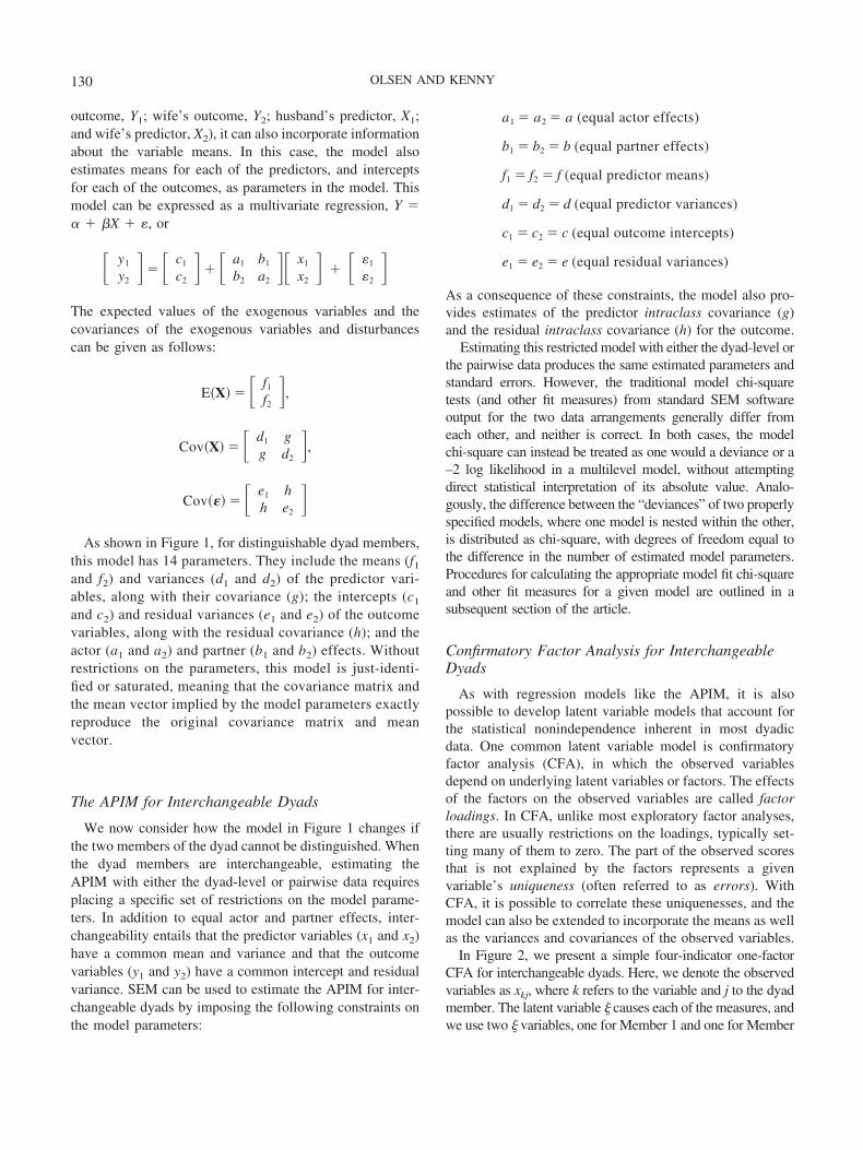
outcome, Y1; wife’s outcome, Y2; husband’s predictor, X1;and wife’s predictor, X2), it can also incorporate informationabout the variable means. In this case, the model alsoestimates means for each of the predictors, and interceptsfor each of the outcomes, as parameters in the model. Thismodel can be expressed as a multivariate regression, Y �� � �X � �, or

� y1

y2� � � c1

c2� � � a1 b1

b2 a2�� x1

x2� � � �1

�2�

The expected values of the exogenous variables and thecovariances of the exogenous variables and disturbancescan be given as follows:

E�X� � � f1

f2�,

Cov�X� � � d1 gg d2

�,

Cov��� � � e1 hh e2

�As shown in Figure 1, for distinguishable dyad members,

this model has 14 parameters. They include the means (f1

and f2) and variances (d1 and d2) of the predictor vari-ables, along with their covariance (g); the intercepts (c1

and c2) and residual variances (e1 and e2) of the outcomevariables, along with the residual covariance (h); and theactor (a1 and a2) and partner (b1 and b2) effects. Withoutrestrictions on the parameters, this model is just-identi-fied or saturated, meaning that the covariance matrix andthe mean vector implied by the model parameters exactlyreproduce the original covariance matrix and meanvector.

The APIM for Interchangeable Dyads

We now consider how the model in Figure 1 changes ifthe two members of the dyad cannot be distinguished. Whenthe dyad members are interchangeable, estimating theAPIM with either the dyad-level or pairwise data requiresplacing a specific set of restrictions on the model parame-ters. In addition to equal actor and partner effects, inter-changeability entails that the predictor variables (x1 and x2)have a common mean and variance and that the outcomevariables (y1 and y2) have a common intercept and residualvariance. SEM can be used to estimate the APIM for inter-changeable dyads by imposing the following constraints onthe model parameters:

a1 � a2 � a (equal actor effects)

b1 � b2 � b (equal partner effects)

f1 � f2 � f (equal predictor means)

d1 � d2 � d (equal predictor variances)

c1 � c2 � c (equal outcome intercepts)

e1 � e2 � e (equal residual variances)

As a consequence of these constraints, the model also pro-vides estimates of the predictor intraclass covariance (g)and the residual intraclass covariance (h) for the outcome.

Estimating this restricted model with either the dyad-level orthe pairwise data produces the same estimated parameters andstandard errors. However, the traditional model chi-squaretests (and other fit measures) from standard SEM softwareoutput for the two data arrangements generally differ fromeach other, and neither is correct. In both cases, the modelchi-square can instead be treated as one would a deviance or a–2 log likelihood in a multilevel model, without attemptingdirect statistical interpretation of its absolute value. Analo-gously, the difference between the “deviances” of two properlyspecified models, where one model is nested within the other,is distributed as chi-square, with degrees of freedom equal tothe difference in the number of estimated model parameters.Procedures for calculating the appropriate model fit chi-squareand other fit measures for a given model are outlined in asubsequent section of the article.

Confirmatory Factor Analysis for InterchangeableDyads

As with regression models like the APIM, it is alsopossible to develop latent variable models that account forthe statistical nonindependence inherent in most dyadicdata. One common latent variable model is confirmatoryfactor analysis (CFA), in which the observed variablesdepend on underlying latent variables or factors. The effectsof the factors on the observed variables are called factorloadings. In CFA, unlike most exploratory factor analyses,there are usually restrictions on the loadings, typically set-ting many of them to zero. The part of the observed scoresthat is not explained by the factors represents a givenvariable’s uniqueness (often referred to as errors). WithCFA, it is possible to correlate these uniquenesses, and themodel can also be extended to incorporate the means as wellas the variances and covariances of the observed variables.

In Figure 2, we present a simple four-indicator one-factorCFA for interchangeable dyads. Here, we denote the observedvariables as xkj, where k refers to the variable and j to the dyadmember. The latent variable � causes each of the measures, andwe use two � variables, one for Member 1 and one for Member

130 OLSEN AND KENNY

2, which are correlated. This correlation can be viewed as alatent variable intraclass correlation. We treat the fourth mea-sure as a marker variable. Finally we correlate the unique-nesses of the same measure across dyad members, and such acorrelation can be viewed as a residual intraclass correlation.

The model can be expressed as a standard factor analysismodel, X � � � �� � �, with specific restrictions on thefactor loadings (�) and indicator means (�), as well aspatterned covariance matrices for the factors (�) and unique-nesses (�).

�x11

x21

x31

x41

x12

x22

x32

x42

� � �abcdabcd

� � �e 0f 0g 01 00 e0 f0 g0 1

���1

�2� � �

�11

�21

�31

�41

�12

�22

�32

�42

�Variables for the first dyad member are above the dottedline, and those for the second member are below the line.Note that for interchangeable dyads, we have set the corre-sponding intercepts and factor loadings equal for the twomembers. The expected values of the factors and the co-variances of the factors and uniquenesses are

E��� � � � � 00 �,

Cov��� � � � � h mm h �,

Cov��� � � � �n 0 0 0 s 0 0 00 p 0 0 0 t 0 00 0 q 0 0 0 u 00 0 0 r 0 0 0 vs 0 0 0 n 0 0 00 t 0 0 0 p 0 00 0 u 0 0 0 q 00 0 0 v 0 0 0 r

�.

Again we have set the appropriate parameters equal for bothdyad members. As shown in the above equations and inFigure 2, this model has 17 unique parameters: a commonfactor variance (h) and factor intraclass covariance (m),along with the common item intercepts (a, b, c, and d),factor loadings (e, f, and g), residual variances (n, p, q, andr), and the residual intraclass covariances (s, t, u, and v) forthe four indicators. Equating the corresponding parametersas shown above with either the dyad-level or pairwise datagives the same set of parameter estimates and standarderrors.

Latent Growth Curve Model for InterchangeableDyads

Some dyadic studies measure variables on multiple occa-sions (Kurdek, 2003). The latent growth curve (LGC) ap-proach (Duncan, Duncan, Strycker, Li, & Alpert, 1999;Singer & Willett, 2003) to longitudinal data describeschange trajectories of dyad members in terms of basicgrowth parameters such as latent intercepts and slopes. InFigure 3, the latent variables �1 and �3 model the intercepts

Figure 2. One-factor four-indicator confirmatory factor analysismodel for interchangeable dyads. The parameters in this modelinclude the three estimated factor loadings (e, f, and g), the factorvariance (h), the factor intraclass covariance (m), the four itemintercepts (a, b, c, and d), the four item measurement error vari-ances (n, p, q, and r), and the four item intraclass error covariances(s, t, u, and v). Zero means for all error and latent variables areomitted to simplify the figure.

Figure 3. Latent growth curve model for interchangeable dyads.Parameters in this model include two estimated factor loadings (gand h), the mean (m) and variance (a) of the latent intercept, themean (n) and variance (b) of the latent slope, four occasion-specific residual variances (p, q, r, and s), four residual intraclasscovariances (t, u, v, and w), the intrapartner (c) and interpartner (d)covariances between the latent intercept and slope, and the intra-class covariances for the latent intercept (e) and slope ( f ).

131SEM WITH INTERCHANGEABLE DYADS

for dyad members 1 and 2, respectively, and �2 and �4 modelthe corresponding slopes. The intercept provides a refer-ence, such as initial status, for an individual’s trajectory ofchange over time, whereas the slope depicts their pattern ofchange. The latent intercepts and slopes are linked to theoccasion-based measures for dyad members 1 (x11, x12, x13,and x14) and 2 (x21, x22, x23, and x24) through model-specificfactor loadings. SEM allows estimation of the average valueof the intercepts (m) and slopes (n), as well as the degree ofvariability in the intercepts (a) and slopes (b) among indi-viduals. It is also possible that individuals’ slopes might becorrelated with their intercepts (c). As seen in Figure 3,there might also be relationships among dyad members’individual growth parameters. For instance, both membersmight be similar in their initial status (e) or be growing ordeclining at similar rates (f). It is also possible that one dyadmember’s slope might be correlated with the other’s inter-cept, and vice versa (d). We also estimate the variability inthe items not due to the underlying intercepts and slopes (p,q, r, and s) and allow correlations of the errors of measurestaken at the same time across dyad members (t, u, v, and w).

This LGC model for interchangeable dyads can again beexpressed as a basic factor analysis model, X � � � �� ��, with specific restrictions on the factor loadings and factormeans, as well as patterned covariance matrices for thefactors and uniquenesses:

�x11

x21

x31

x41

x12

x22

x32

x42

� � �00000000

� � �1 0 0 01 1 0 01 g 0 01 h 0 00 0 1 00 0 1 10 0 1 g0 0 1 h

���1

�2

�3

�4

� � ��1

�2

�3

�4

�5

�6

�7

�8

�In the LGC model, unlike the CFA model, the item inter-cepts are generally fixed at zero, relying on the estimatedslopes and intercepts to account for the mean structure ofthe data. The LGC model presented here is sometimescalled the unspecified LGC model (see Duncan et al., 1999).It differs from more typical LGC models in that not all ofthe slope factor loadings are fixed at specified numericconstants. In the typical LGC model, these constants areused to indicate the timing of the measurement occasionswith respect to one of the measures that is chosen as areference measure. For example, with four equally spacedoccasions where the first measure is treated as the reference,a linear trajectory over time could be modeled in the latentslope by fixing the four slope factor loadings to the values0, 1, 2, and 3. The unspecified LGC model estimates thelatter two coefficients from the data, allowing departurefrom the linear pattern.2 However, the estimated loadings (gand h) are constrained to be the same for both dyad mem-

bers. The expected values of the latent slope and interceptfactors and the covariances of the factors and the unique-nesses are

E��� � � � �mnmn�,

Cov��� � � � �a c e dc b d fe d a cd f c b

�,

Cov��� � � � �p 0 0 0 t 0 0 00 q 0 0 0 u 0 00 0 r 0 0 0 v 00 0 0 s 0 0 0 wt 0 0 0 p 0 0 00 u 0 0 0 q 0 00 0 v 0 0 0 r 00 0 0 w 0 0 0 s

�In this model, there is a common intercept (m) and slope (n),along with their variances (a and b), the intrapartner andcross-partner covariances between intercept and slope (cand d), the intraclass covariances between the intercepts (e)and the slopes ( f ), the estimated slope factor loadings (gand h), and the residual variances (p, q, r, and s) and dyadicresidual intraclass covariances (t, u, v, and w) at each of thefour time periods.

The APIM, CFA, and LGC models are examples of abroad class of statistical models for dyadic data that can bereadily estimated for interchangeable as well as distinguish-able dyads using our proposed SEM approach. Properlyspecified models for interchangeable dyads that are nestedcan be compared using traditional chi-square differencetests. However, a complete treatment of model fit and modelcomparisons for our proposed SEM approach requires someadditional background and development.

Model Fit and Model Comparisons

SEM estimates a set of model parameters that minimizesthe discrepancy between the model-implied and the ob-served covariance matrices and mean vectors (Kline, 2005).With dyads that are distinguishable, data from the dyad-level arrangement can be analyzed straightforwardly, andtraditional SEM procedures for identifying and estimating

2 The interpretation of the slope and the covariance between theslope and intercept is slightly more complicated in the unspecifiedLGC model (see Bollen & Curran, 2006, pp. 98–102).

132 OLSEN AND KENNY

models, and assessing model fit, can be used. However, ourmethod for analyzing data from interchangeable dyads re-quires some modifications to the standard SEM approach.

With dyadic data on a set of k variables for each of twodyad members, giving 2k means and a 2k by 2k covariancematrix, we can arrange the observed mean vector X� andcovariance matrix S so that the first member’s variablesprecede the second member’s variables, with the variablesordered in the same way for both members:

X� � � X� 1

X� 2

.�,

S � � S11 S12

S21 S22�

Here, X� 1 and X� 2 are the means; S11 and S22 are the intra-partner covariance matrices for the first and second dyadmembers, respectively; and S21 and S12 contain the cross-partner covariances. For both the dyad-level and the pair-wise data, X� and S provide the basis for our approach toSEM for interchangeable dyads.

Within SEM, fit assessment and model comparisons haveused an independence or null model. The traditional nullmodel fits only the means and variances, constraining thecovariances to zero. Implicitly, models are also comparedwith a best fitting or saturated model having perfect fit andexactly reproducing the original covariance matrix andmean vector. Theoretically, any proposed model must fit atleast as well as the independence model and can fit no betterthan the saturated model. The traditional chi-square test ofmodel fit compares the fit of a candidate model with that ofthe saturated model, and both the saturated and null modelsare used to define basic reference points for fit when devel-oping the various alternative fit measures available fromSEM software. The primary task with interchangeable dy-ads is to develop the appropriate new null and saturatedmodels.

For interchangeable dyads, the model-implied mean vec-tor for both the new null (I–NULL, for “interchangeablenull”) and saturated (I–SAT, for “interchangeable satu-rated”) models can be partitioned into two subvectors,�IN � �IS � �1��2 �, with the condition that �1

� �2. As with the observed covariance matrix, the model-implied covariance matrix, �IS, for the I–SAT model can bepartitioned into four symmetrical submatrices, with sub-scripts referring to the dyad members:

�IS � � �11 �12

�21 �22�

This expression holds for both the dyad-level and pairwise dataarrangements. In addition to equal means, the I–SAT model

requires that the two individual dyad member covariancesubmatrices be equal, �11 � �22, and that the submatrix ofcross-covariances between dyad members be symmetrical,�12 � �21. The I–SAT model has k(k � 2) parameters andk(k � 1) degrees of freedom. Both dyad-level and pairwisedata give the same model-implied covariance matrix forI–SAT. For the pairwise data, the model-implied covariancematrix under I–SAT is also identical to the original pairwisecovariance matrix. This is because the symmetrical regularitiesentailed by the interchangeability constraints are already em-bedded in the construction of the pairwise data.

Starting from I–SAT, the model-implied covariance ma-trix under I–NULL further requires that �11 and �22 bediagonal and that �12 � �21 � 0. By itself, the lattercondition provides a general test of nonindependence. TheI–NULL model has 2k parameters, k unique means and kunique variances, and k(2k � 1) degrees of freedom.

A properly specified interchangeable model must fit atleast as well as the I–NULL model and can fit no better thanthe I–SAT model. Nested interchangeable models can becompared using standard chi-square difference tests,whereas nonnested but appropriately specified interchange-able models can be compared using standard informationtheory fit criteria (e.g., Akaike or Bayesian informationcriteria). Because all interchangeable models are nestedwithin I–SAT, model fit for a given model can be assessedby constructing a traditional chi-square difference test com-paring the hypothesized model with I–SAT.

The I–NULL and I–SAT models for k variables measuredon each of two dyad members can be estimated with asimple means model, X � � �, having a speciallypatterned covariance matrix for the errors. For four mea-sured variables, this can be given as

�x11

x21

x31

x41

x12

x22

x32

x42

� � �vwxyvwxy

� � ��11

�21

�31

�41

�12

�22

�32

�42

�with

Cov(�) � � � �a e f g l p q re b h i p m s tf h c j q s n ug i j d r t u ol p q r a e f gp m s t e b h iq s n u f h c jr t u o g i j d

� .

133SEM WITH INTERCHANGEABLE DYADS

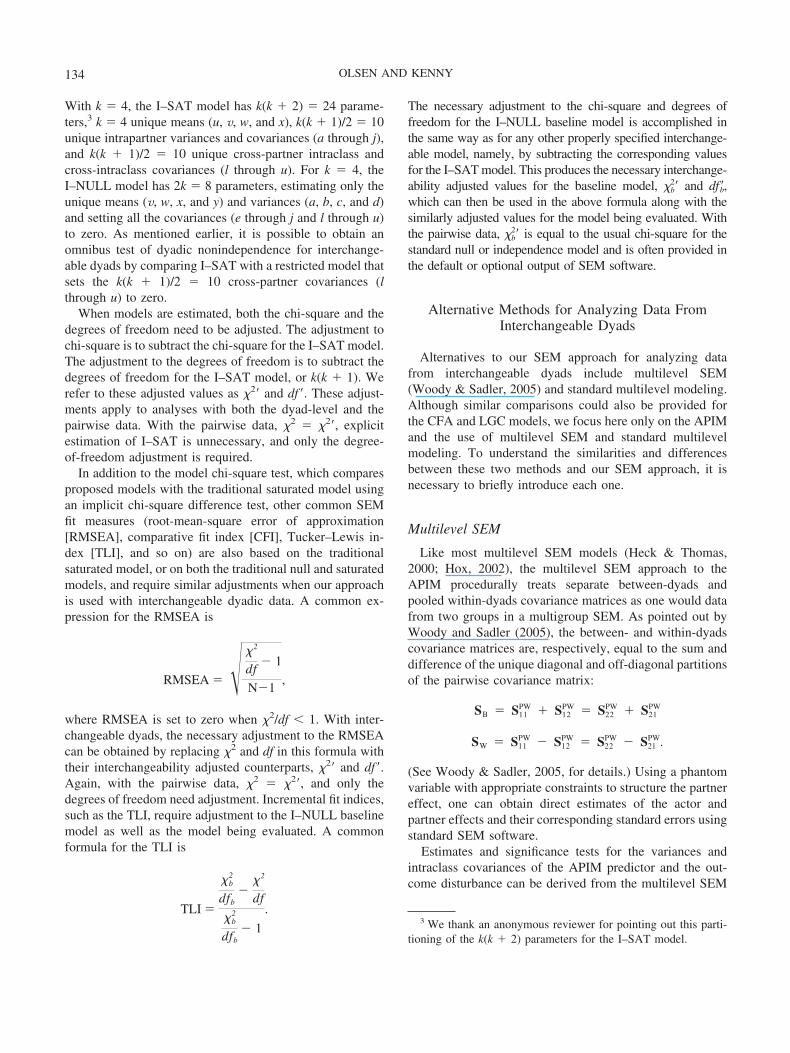
With k � 4, the I–SAT model has k(k � 2) � 24 parame-ters,3 k � 4 unique means (u, v, w, and x), k(k � 1)/2 � 10unique intrapartner variances and covariances (a through j),and k(k � 1)/2 � 10 unique cross-partner intraclass andcross-intraclass covariances (l through u). For k � 4, theI–NULL model has 2k � 8 parameters, estimating only theunique means (v, w, x, and y) and variances (a, b, c, and d)and setting all the covariances (e through j and l through u)to zero. As mentioned earlier, it is possible to obtain anomnibus test of dyadic nonindependence for interchange-able dyads by comparing I–SAT with a restricted model thatsets the k(k � 1)/2 � 10 cross-partner covariances (lthrough u) to zero.

When models are estimated, both the chi-square and thedegrees of freedom need to be adjusted. The adjustment tochi-square is to subtract the chi-square for the I–SAT model.The adjustment to the degrees of freedom is to subtract thedegrees of freedom for the I–SAT model, or k(k � 1). Werefer to these adjusted values as 2� and df �. These adjust-ments apply to analyses with both the dyad-level and thepairwise data. With the pairwise data, 2 � 2�, explicitestimation of I–SAT is unnecessary, and only the degree-of-freedom adjustment is required.

In addition to the model chi-square test, which comparesproposed models with the traditional saturated model usingan implicit chi-square difference test, other common SEMfit measures (root-mean-square error of approximation[RMSEA], comparative fit index [CFI], Tucker–Lewis in-dex [TLI], and so on) are also based on the traditionalsaturated model, or on both the traditional null and saturatedmodels, and require similar adjustments when our approachis used with interchangeable dyadic data. A common ex-pression for the RMSEA is

RMSEA � � 2

df� 1

N�1,

where RMSEA is set to zero when 2/df � 1. With inter-changeable dyads, the necessary adjustment to the RMSEAcan be obtained by replacing 2 and df in this formula withtheir interchangeability adjusted counterparts, 2� and df �.Again, with the pairwise data, 2 � 2�, and only thedegrees of freedom need adjustment. Incremental fit indices,such as the TLI, require adjustment to the I–NULL baselinemodel as well as the model being evaluated. A commonformula for the TLI is

TLI �

b2

dfb�

2

df

b2

dfb� 1

.

The necessary adjustment to the chi-square and degrees offreedom for the I–NULL baseline model is accomplished inthe same way as for any other properly specified interchange-able model, namely, by subtracting the corresponding valuesfor the I–SAT model. This produces the necessary interchange-ability adjusted values for the baseline model, b

2� and df�b,which can then be used in the above formula along with thesimilarly adjusted values for the model being evaluated. Withthe pairwise data, b

2� is equal to the usual chi-square for thestandard null or independence model and is often provided inthe default or optional output of SEM software.

Alternative Methods for Analyzing Data FromInterchangeable Dyads

Alternatives to our SEM approach for analyzing datafrom interchangeable dyads include multilevel SEM(Woody & Sadler, 2005) and standard multilevel modeling.Although similar comparisons could also be provided forthe CFA and LGC models, we focus here only on the APIMand the use of multilevel SEM and standard multilevelmodeling. To understand the similarities and differencesbetween these two methods and our SEM approach, it isnecessary to briefly introduce each one.

Multilevel SEM

Like most multilevel SEM models (Heck & Thomas,2000; Hox, 2002), the multilevel SEM approach to theAPIM procedurally treats separate between-dyads andpooled within-dyads covariance matrices as one would datafrom two groups in a multigroup SEM. As pointed out byWoody and Sadler (2005), the between- and within-dyadscovariance matrices are, respectively, equal to the sum anddifference of the unique diagonal and off-diagonal partitionsof the pairwise covariance matrix:

SB � S11PW � S12

PW � S22PW � S21

PW

SW � S11PW � S12

PW � S22PW � S21

PW.

(See Woody & Sadler, 2005, for details.) Using a phantomvariable with appropriate constraints to structure the partnereffect, one can obtain direct estimates of the actor andpartner effects and their corresponding standard errors usingstandard SEM software.

Estimates and significance tests for the variances andintraclass covariances of the APIM predictor and the out-come disturbance can be derived from the multilevel SEM

3 We thank an anonymous reviewer for pointing out this parti-tioning of the k(k � 2) parameters for the I–SAT model.

134 OLSEN AND KENNY

estimates and standard errors of the between- and within-dyads variances for the predictor and the outcome distur-bance using formulas given in Woody and Sadler (2005).Neither the predictor mean nor the outcome intercept areincluded as model parameters in multilevel SEM.

With the multilevel SEM approach to the APIM forinterchangeable dyads, I–SAT is identical to the “ordi-nary” saturated model. Because of this, the model chi-square, along with its degrees of freedom, and the RM-SEA require no adjustment as they do with our SEMapproach. The I–NULL model can be estimated by set-ting the actor and partner effects to zero and equating thepredictor variances and residual variances across“groups.” This is the model that should be used, ratherthan the default baseline model employed by standardSEM software when computing incremental fit indices(e.g., CFI or TLI).

The multilevel SEM approach of Woody and Sadler(2005) uses appropriate parameter restrictions across the

between- and within-dyads models, along with the factthat the data are balanced (all groups are of size 2), toproduce full-information maximum likelihood estimatesthat are equivalent to the corresponding estimates fromour approach. Because of the model restrictions, many ofthe problems traditionally seen in multilevel SEM withsmall groups (see Hox & Maas, 2001) are lessened. Still,in light of the experience with multilevel SEM and mul-tilevel regression, further research is needed with bothmethods to examine whether and under what circum-stances program nonconvergence, inadmissible solutions,or bias in estimated parameters or standard errors mightbe encountered.

Standard Multilevel Analysis

The APIM for interchangeable dyads can also be esti-mated as a standard multilevel model. Kenny, Kashy, and

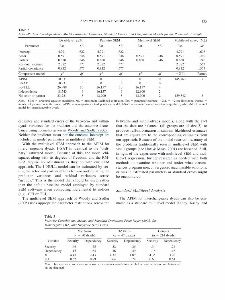
Table 2Actor–Partner Interdependence Model Parameter Estimates, Standard Errors, and Comparison Models for the Roommate Example

Parameter

Dyad-level SEM Pairwise SEM Multilevel SEM Multilevel mixed (ML)

Est. SE Est. SE Est. SE Est. SE

Intercept 4.791 .622 4.791 .622 4.791 .606Actor 0.591 .246 0.591 .246 0.591 .246 0.591 .240Partner 0.888 .246 0.888 .246 0.888 .246 0.888 .240Residual variance 2.382 .577 2.382 .577 2.382 .563Partial covariance 0.812 .577 0.812 .577 0.812 .563

Comparison model 2 df 2 df 2 df �2LL Parms.

APIM 10.831 6 0 6 0 0 145.763 5I–SAT 10.831 6 0 6 0 0I–NULL 26.988 10 16.157 10 16.157 4Independence 18.543 6 16.157 6 12.900 2No actor or partner 23.731 8 12.900 8 12.900 2 159.342 3

Note. SEM � structural equation modeling; ML � maximum likelihood estimation; Est. � parameter estimate; �2LL � �2 log likelihood; Parms. �number of parameters in the model; APIM � actor–partner interdependence model; I–SAT � saturated model for interchangeable dyads; I–NULL � nullmodel for interchangeable dyads.

Table 3Pairwise Correlations, Means, and Standard Deviations From Neyer (2002) forMonozygotic (MZ) and Dizygotic (DZ) Twins

Variable

MZ twins(n � 80 dyads)

DZ twins(n � 47 dyads)

Couples(n � 214 dyads)

Security Dependency Security Dependency Security Dependency

Security .66 .25 .32 .36 .34 .24Dependency .15 .64 .36 .49 .18 .46M 4.48 2.43 4.32 1.89 4.35 3.20SD 0.52 0.89 0.64 0.74 0.60 0.61

Note. Intrapartner correlations are above, cross-partner correlations are below, and intraclass correlations areon the diagonal.

135SEM WITH INTERCHANGEABLE DYADS

Cook (2006) use a mixed model, Y � X� � �, with thefollowing error covariance matrix specification:

� y1

y2� � � 1 x1 x2

1 x2 x1�� c

ab� � ��1

�2� ,

Cov(�)��eh e�.

The specification, commonly called compound symmetry,gives a common residual variance for the two dyad membersalong with a corresponding intraclass covariance. Note that �1

and �2 are the errors in the equation for Members 1 and 2. Thefive parameters of this model are the common intercept (c),actor (a), and partner (b) effects, along with the residual vari-ance (e) and covariance (h). In contrast to our SEM approach,the mean, variance, and intraclass covariance of the predictorvariable are not explicitly estimated as part of the standardmultilevel APIM model, nor can they be derived from esti-mated model parameters using side calculations, as they canwith multilevel SEM.

Examples

In this section we provide examples of using the APIM,CFA, and LGC models with data from interchangeable

dyads, along with selected comparisons of our approach tomultilevel SEM and standard multilevel modeling.

Example 1: Estimating the APIM forInterchangeable Dyads

Just as the unconstrained APIM is just-identified orsaturated for distinguishable members, the interchange-able APIM is equivalent to I–SAT. Although the fit of themodel cannot be tested, the parameter estimates andcorresponding standard errors address issues of centralimportance to dyadic researchers. Also, certain submod-els (e.g., equal actor and partner effects) may be oftheoretical interest. Using fictitious data for 20 roommatedyads from chapter 7 of Kenny et al. (2006), our ap-proach to SEM for interchangeable dyads gives the sameestimates and standard errors (see Table 2) for both thedyad-level and pairwise data.

The multilevel SEM also gives the same estimates andstandard errors for the actor and partner effects, andestimates and standard errors of the residual variance andcovariance can be obtained from formulas given inWoody and Sadler (2005). The multilevel mixed modelwith maximum likelihood estimation gives the same es-timates as our SEM approach, but the standard errors areslightly smaller. Although our assessment is limited tothe specific models that we have estimated, there areseveral possibilities we might consider for the slightdifferences we have observed in the standard errors whenusing multilevel modeling and SEM to estimate theAPIM. Bauer (2003) and Curran (2003) have also dis-cussed the equivalence of certain other kinds of multi-level and SEM models.

Although not shown in Table 2, estimates and standarderrors for the mean, variance, and intraclass covarianceof the predictor are also available from the SEM outputfor the dyad-level and pairwise data and from additionalside calculations for the multilevel SEM. Although theAPIM is just-identified for interchangeable dyadic dataand has fit identical to I–SAT, it is instructive to compare

Table 4Expanded Pairwise Correlations, Means, and StandardDeviations for Monzygotic Twins

Dyadmember X Y X� Y�

X — .25 .64 .15Y .25 — .15 .66X� .64 .15 — .25Y� .15 .66 .25 —M 4.48 2.43 4.48 2.43SD 0.52 0.89 0.52 0.89

Note. X� and Y� are measurements of the partner.

Table 5APIM Regression Coefficients for Interchangeable Dyads With the Neyer (2002) DataUsing SEM as Reported by Neyer

Dyad type

Dependency 3 Security Security 3 Dependency

Actor Partner Actor Partner

Neyer SEM Neyer SEM Neyer SEM Neyer SEM

Monozygotic (n � 80) .15*** .15*** .00 �.01 .45*** .46*** �.03 �.05Dizygotic (n � 47) .21*** .21* .22*** .21* .31*** .32** .32*** .32**Couples (n � 214) .20*** .20*** .09** .09 .20*** .21*** .12*** .11*

Note. APIM � actor–partner interdependence model; SEM � structural equation modeling.* p � .05. ** p � .01. *** p � .001.

136 OLSEN AND KENNY

it with I–NULL, the traditional independence model, anda model with no actor or partner effects (see Table 2). Allthree SEM methods provide the correct chi-square dif-ference test comparing the APIM with I–NULL, 2(4) �16.157. However, only the multilevel SEM gives thecorrect unadjusted degrees of freedom for the fit of APIM(0), I–SAT (0), and I–NULL (4) to interchangeable dy-adic data. Both the dyad-level and pairwise SEM meth-ods require subtraction of the chi-square and degrees offreedom from the I–SAT model in order to properlyinterpret the fit of APIM and I–NULL.

Example 2: Multiple Group SEM Using the APIMWith Interchangeable Dyads

The APIM can be simultaneously applied to two or moregroups or sets of interchangeable dyads. Neyer (2002) usedKenny’s (1996) pooled regression method for estimating theAPIM separately for monozygotic (MZ) and dizygotic (DZ)twin pairs, as well as for young romantic couples. Membersof the romantic couple dyads were treated as interchange-able after preliminary tests established homogeneity of thevariances and covariances for husbands and wives. Neyerprovided pairwise correlations as well as means and stan-dard deviations for attachment security and dependency forthe MZ, DZ, and couple dyads (see Table 3). AlthoughTable 3 provides a compact representation of the pairwisedata, modeling with SEM software requires the expansionand structured redundancy as shown in Table 4 for the MZdyads. Applying interchangeability restrictions to the ex-panded matrices for MZ, DZ, and couple dyads allows theuse of SEM to estimate the model.

With both security and dependency treated in turn as thedependent variable, results from Neyer’s (2002) pooledregression analysis and I–SEM with pairwise data are givenin Table 5. The corresponding coefficients are very similar,

but with some small differences in the reported statisticalsignificance levels. Neyer further compared actor and part-ner effects across the three types of dyads using Z tests ofthe differences between independent standardized path co-efficients. Similar tests of differences between the corre-sponding unstandardized coefficients were conducted withSEM using Amos 5.0 (Arbuckle, 2003).

No statistically significant actor effect differences werefound with either security or dependency as the dependentvariable. For attachment security, a significant differencebetween the MZ and DZ partner effects was found (Z �2.20). For attachment dependency, we found differencesbetween the MZ and DZ dyads (Z � 2.12) but not betweenthe MZ and couple dyads (Z � 1.13). Imposing appropriateparameter constraints across groups in SEM allows for thetesting of group differences in the means, intercepts, vari-ances, or intraclass covariances, as well as the regressioncoefficients.

Example 3: A CFA Model for InterchangeableDyads

Same-sex twins are an example of interchangeable pairs.A common error in many exploratory and confirmatoryfactor analyses of data from twins is to ignore their pairing,

Table 6Correlations, Means, and Standard Deviations for Male Monozygotic Twin Pairs (n � 137)

Variable x11 x21 x31 x41 x12 x22 x32 x42 M SD

x11 — .358 .335 .461 .407 .231 .130 .219 3.058 0.622x21 .380 — .431 .404 .231 .444 .171 .196 2.523 0.618x31 .351 .483 — .318 .130 .171 .092 .114 2.908 0.611x41 .531 .386 .385 — .219 .196 .114 .355 3.119 0.674

-------------------------------------------------------------------------------------x12 .411 .161 .142 .228 — .358 .335 .461 3.058 0.622x22 .313 .453 .266 .245 .348 — .431 .404 2.523 0.618x32 .118 .080 .092 .099 .323 .381 — .318 2.908 0.611x42 .214 .148 .129 .357 .403 .431 .256 — 3.119 0.674M 3.042 2.571 2.903 3.095 3.074 2.474 2.913 3.144SD 0.579 0.626 0.607 0.653 0.662 0.605 0.615 0.694

Note. Dual-entry correlations are above and dyad-level correlations are below the diagonal. x1 � reappraisal;x2 � foresight; x3 � insight; x4 � self-directedness. Second subscript refers to twin number, 1 and 2.

----

----

----

----

----

---

Table 7Chi-Square Tests for the CFA Model forMale Monozygotic Twins

Model df 2 df � 2� RMSEA TLI

Null 36 283.210 16 261.519 .336 .000CFA 27 34.392 7 12.701 .077 .977Saturated 20 21.691

Note. CFA � confirmatory factor analysis; RMSEA � root-mean-squareerror of approximation; TLI � Tucker–Lewis index.

137SEM WITH INTERCHANGEABLE DYADS

treating them as if they were 2n independently sampledindividuals. Such an analysis fails to consider the potentialintraclass correlation of either the factors or the unique-nesses. Moreover, sometimes these correlations are of cen-tral research interest. For example, behavior genetic analy-ses of twin data typically use differences between theintraclass correlations of MZ and DZ twins to estimate traitheritability.

We use adult male identical twin pairs from the MidlifeDevelopment Study (Brim et al., 2003) to illustrate appro-priate analysis of data from interchangeable pairs. Our anal-yses are a methodological demonstration, not a substantivebehavior genetic model. We restricted our analysis to 137male MZ twin pairs providing complete data on four, four-item personality variables: reappraisal (e.g., “I find I usuallylearn something meaningful from a difficult situation”),foresight (e.g., “I am good at figuring out how things willturn out”), insight (e.g., “I try to make sense of things thathave happened to me”), and self-directedness (e.g., “I like tomake plans for the future”). The correlations, means, andstandard deviations for both the dyad-level and pairwisedata are given in Table 6.

In Table 7, for both the dyad-level and pairwise data, thefit of the CFA model is tested using the chi-square differ-ence between the CFA and I–SAT models. The fit of modelis acceptable, 2(7)� � 12.701, p � .08. As seen in Table 8,both the dyad-level and pairwise data give the same esti-mates and standard errors. All parameters are statisticallysignificant except the residual intraclass correlation forinsight.

For the factor loadings, these results are also identical tothose from multilevel SEM. With multilevel SEM, how-ever, estimates and tests of the variances and intraclasscovariances of the factors and uniquenesses require addi-tional side calculations using the Woody and Sadler (2005)formulas. So far as we know, this model cannot be esti-mated by multilevel modeling.

LISREL syntax for the CFA model using the pairwise ordual-entry data are available on the Web at http://dx.doi.org/10.1037/1082-989X.11.2.127.supp. It also contains the nec-essary syntax to estimate the corresponding null and satu-rated models. The same syntax is used for the dyad-level

data, replacing the correlations, means, and standard devi-ations with the dyad-level counterparts from Table 6. (Be-cause our estimates use Amos 5.0 with raw data, estimatesproduced by LISREL will differ slightly owing to roundingerror in the correlations, means, and standard deviations.)

Example 4: An LGC Model for InterchangeableDyads

Duncan et al. (1999, chap. 9) used multilevel SEM and amethod much like our dyad-level SEM to estimate latentgrowth curves for alcohol use over four time periods fromfamilies containing two, three, or four members.4 We useonly the data from the two-member families to illustrate theapplication to the dyadic case. Also, instead of using onlyfixed factor loadings to define the basis for the time scale,we freely estimate two of the basis factor loadings. Thecommon factor loadings, uniquenesses, and residual intra-class covariances are given in Table 9, and the commonlatent curve means, variances, and intraclass and intercept–slope covariances are given in Table 10. We note that thereis variance in both slope and intercept, and the correlationbetween dyad members’ slopes is somewhat stronger thanfor intercepts (.47 vs. .27), although both are statisticallysignificant.

Using the dyad-level data, the chi-square and degrees offreedom for the I–NULL, I–SAT, and interchangeable latentcurve models are given in Table 11. We also give thecorrected chi-squares and degrees of freedom. The fit of theproposed latent curve model is assessed with the 2� adjust-ment (44.626 � 23.913 � 20.713) having (26 � 20 � 6)degrees of freedom. The adjusted RMSEA and TLI for thismodel are .100 and .964, respectively. When the order of thedyad members is randomly permuted, all of the parameterestimates and standard errors remain the same, but all of thechi-square values shift. Specifically, the I–SAT modelchanges. However, for this scrambled data set, the adjustedchi-square and degrees of freedom are the same as before, asare the RMSEA and TLI using the adjusted values.

4 The data and SEM software code provided by Duncan et al.(1999) can be found at http://www.ori.org/methodology/.

Table 8Interchangeable CFA Estimates (and Standard Errors) for 137 Male Monozygotic Twin Pairs

Variable Loading Mean Variance Covariance

Factor 0.194 (0.042) 0.093 (0.030)Reappraisal 0.864 (0.128) 3.058 (0.044) 0.236 (0.028) 0.077 (0.026)Foresight 0.880 (0.129) 2.523 (0.044) 0.223 (0.028) 0.082 (0.026)Insight 0.775 (0.119) 2.908 (0.039) 0.254 (0.027) �0.005 (0.025)Self-Directedness 1.000 3.119 (0.048) 0.261 (0.034) 0.079 (0.030)

Note. CFA � confirmatory factor analysis.

138 OLSEN AND KENNY

Limitations

In this section, we briefly review the major practical andstatistical limitations of the approach that we have devel-oped. We begin with sample size requirements. For theabsolute minimum number of cases, the number of dyadsplus one must be twice as great as the number of variablesin the model. We note that the effective sample size issomewhere between the number of dyads and the number ofindividuals. For dyads, the effective sample size can beestimated by dividing the number of individuals by one plusthe average intraclass correlation (see Snijders & Bosker,1999, p. 23).

One practical limitation of our approach is that it doesrequire careful attention to detail in the analysis. If thedyad-level method is used, numerous equality constraintsmust be made. Also, corrections must be made to model fitindices.

Additionally, all of the assumptions required within SEMare required for our approach. In particular, multivariatenormality is usually assumed. Checks should be made fornormality, and if the data are severely nonnormal, somecorrective strategy should be adopted. Additionally, it isassumed that functional relationships are linear. Finally, and

most important, SEM requires that the model be correctlyspecified. Care in design, measurement, and theoreticalanalysis should be undertaken to ensure that there is mini-mal specification error.

Conclusion

We have demonstrated that SEM can be used to estimatemodels for data from interchangeable dyads. Contrary to theview that SEM is unsuitable for indistinguishable dyads, wehave presented a relatively straightforward approach to thisproblem by imposing equality constraints on correspondingmodel parameters across dyad members and by making asimple adjustment to chi-square and degrees of freedom.

We have shown how to apply this approach with bothdyad-level and weighted pairwise data. SEM with both dataarrangements yields identical results for the desired modelparameters and standard errors. We have described modeltesting procedures and illustrated the necessary adjustmentsto fit measures with both dyad-level and pairwise data.These models, along with multilevel SEM models thatjointly analyze separate between- and within-dyads covari-ance matrices (Woody & Sadler, 2005), constitute viableapproaches to the analysis of data from interchangeabledyads within SEM.

Our approach exploits the ability of SEM to estimatelatent variable and path models, to model correlated mea-surement errors and equation disturbances, and to easilyimpose equality and other constraints on model parameters.Where equivalent models are estimable, it gives the same

Table 9Interchangeable Latent Growth Curve Factor Loadings, Uniquenesses, and Residual IntraclassCovariances With Standard Errors

Occasion

Factor loadings Uniquenesses Intraclass covariances

Estimate SE Estimate SE Estimate SE

1 0 —a .803 0.141 0.018 0.1342 1 —a 1.208 0.106 0.015 0.1053 2.738 0.277 1.525 0.146 0.223 0.1404 3.257 0.331 1.446 0.175 0.057 0.166

a Parameter fixed.

Table 10Latent Curve Means, Variances, and Intraclass and Intercept–Slope Covariances With Standard Errors

Parameter Estimate SE

InterceptMean 2.639 0.095Variance 2.878 0.244Intraclass covariance 0.781 0.242

SlopeMean 0.562 0.065Variance 0.165 0.046Intraclass covariance 0.078 0.031

Intrapartner intercept–slope covariance �0.135 0.067Cross-partner intercept–slope covariance �0.020 0.061

Note. See Bollen and Curran (2006, pp. 98–102) for more information onthe interpretation of these effects.

Table 11Model Comparisons for Original andRandomly Permuted Dyads

Model Parameters 12 2

2 df 2� df �

Null 8 1,135.835 1,129.347 36 1,111.922 16Latent curve 18 44.626 38.138 26 10.713 6Saturated 24 23.913 17.425 20

Note. 12 is for the original data; 2

2 is for data where the order ofapproximately half of the dyads was randomly exchanged.

139SEM WITH INTERCHANGEABLE DYADS

parameter estimates as traditional multilevel modeling.Where the same parameters can be estimated, it gives thesame estimates of the parameters and standard errors asmultilevel SEM. However, unlike standard multilevel anal-ysis, it can handle very general latent variable structures andpath models. Unlike multilevel SEM, it can model the meanstructure as well as the covariance structure of the data andcan more directly provide estimates and tests of the desiredmodel parameters, as well as simpler procedures for obtain-ing standardized estimates and R2 values. Compared withmultilevel SEM, we believe our approach also has simplerdata preparation and is easier to parameterize. On the otherhand, multilevel SEM does not require adjustment of thechi-square or RMSEA statistics. With multilevel SEM,however, incremental fit measures such as the TLI alsorequire estimation of an alternative null model, along withadjustments similar to those needed when our approach isused with dyad-level data.

We have described a general method that can be usedwith almost any SEM software program capable of analyz-ing the mean structure as well as the covariance structure ofthe data. Additional SEM software features that could sim-plify the use of our method include the ability to specifyadjusted degrees of freedom (such as in Mx) and the abilityto designate specified alternative models in place of thetraditional baseline and saturated models for the purpose offit measure calculation (see also Widaman & Thompson,2000).

Having seen that our approach gives essentially equiva-lent results for both dyad-level and pairwise data, one mightask under what circumstances each data arrangement mightbe preferred. Each has its advantages. The double-entered orpairwise approach involves simpler adjustments to fit mea-sures and does not require separate estimation of the chi-square statistics for the appropriate baseline (I–NULL) andsaturated (I–SAT) models. However, in terms of data prep-aration, the (single-entered) dyad-level approach is simplerto set up. Also, with both distinguishable and indistinguish-able dyads in the same study (e.g., same- and opposite-sexDZ twins), the dyad-level approach would seem to be morepractical, as the method is more directly comparable to thetraditional analyses of distinguishable dyads. In general,though, the choice is largely a matter of convenience to theresearcher.

To illustrate the generality of the basic strategy, we haveused dyadic regression, CFA, and growth curve models.Because in each case, we impose interchangeability restric-tions on models initially suitable for distinguishable dyads,we emphasize the basic coherence of these methods for bothtypes of dyads. There are several ways in which the proce-dures outlined here can be extended and generalized. Al-though we have focused on dyads, it is also possible tostraightforwardly extend our approach to triads or larger

groups. We have shown how latent curve models can beused with longitudinal data from interchangeable dyads, butour approach could also be applied to traditional autoregres-sive or panel models for repeatedly measured dyadic data.Our presentation has been based on standard assumptions ofinterval measurement and multivariate normality, but itcould be easily extended to handle dichotomous or ordinaldata using appropriate SEM software such as MPlus.

SEM provides an integrated and consistent strategy formodel estimation and testing with dyadic data. Rather thangathering together results from disparate methods and anal-yses (repeated measures analysis of variance, factor analy-sis, intraclass correlation, multilevel regression, and so on),we can estimate parameters and compare models within aunified and coherent framework. Although the examples wehave presented are relatively simple, they provide importantbuilding blocks for more complex and interesting models.

References

Arbuckle, J. L. (2003). Amos 5.0 update to the Amos user’s guide.Chicago: Smallwaters.

Bauer, D. J. (2003). Estimating multilevel linear models as struc-tural equation models. Journal of Educational and BehavioralStatistics, 28, 135–167.

Bollen, K. A., & Curran, P. J. (2006). Latent curve models: Astructural equation perspective. New York: Wiley.

Brim, O. G., Baltes, P. B., Bumpass, L. L., Cleary, P. D., Feath-erman, D. L., Hazzard, W. R., et al. (2003). National Survey ofMidlife Development in the United States (MIDUS), 1995–1996[Computer file] (2nd ICPSR version). Ann Arbor, MI: Interuni-versity Consortium for Political and Social Research [Distribu-tor].

Campbell, L., & Kashy, D. A. (2002). Estimating actor, partner,and interaction effects for dyadic data using PROC MIXED andHLM: A user-friendly guide. Personal Relationships, 9, 327–342.

Cook, W. L. (1994). A structural equation model of dyadic rela-tionships within the family system. Journal of Consulting andClinical Psychology, 62, 500–509.

Curran, P. J. (2003). Have multilevel models been structural equa-tion models all along? Multivariate Behavioral Research, 38,529–559.

Duncan, T. E., Duncan, S. C., Strycker, L. A., Li, F., & Alpert, A.(1999). An introduction to latent growth curve modeling. Mah-wah, NJ: Erlbaum.

Gonzalez, R., & Griffin, D. (2002). Modeling the personality ofdyads and groups. Journal of Personality, 70, 901–924.

Griffin, D., & Gonzalez, R. (1995). Correlational analysis ofdyad-level data in the exchangeable case. Psychological Bulle-tin, 118, 430–439.

Heck, R. H., & Thomas, S. L. (2000). An introduction to multilevelmodeling techniques. Mahwah, NJ: Erlbaum.

140 OLSEN AND KENNY

Hox, J. (2002). Multilevel analysis: Techniques and applications.Mahwah, NJ: Erlbaum.

Hox, J. J., & Maas, C. J. M. (2001). The accuracy of multilevelstructural equation modeling with pseudobalanced groups andsmall samples. Structural Equation Modeling, 8, 157–174.

Kenny, D. A. (1996). Models of non-independence in dyadicresearch. Journal of Social and Personal Relationships, 13,279–294.

Kenny, D. A., Kashy, D. A., & Cook, W. L. (2006). The analysisof dyadic data. New York: Guilford Press.

Kline, R. (2005). Principles and practice of structural equationmodeling (2nd ed.). New York: Guilford Press.

Kurdek, L. A. (2003). Methodological issues in growth-curveanalyses with married couples. Personal Relationships, 10, 235–266.

Muthen, L. K., & Muthen, B. O. (2001). Mplus user’s guide. LosAngeles: University of California.

Neyer, F. J. (2002). The dyadic interdependence of attachmentsecurity and dependency: A conceptual replication across older

twin pairs and younger couples. Journal of Social and PersonalRelationships, 19, 483–503.

Rowe, D. C., & Cleveland, H. H. (1996). Academic achievementin Blacks and Whites: Are the developmental processes similar?Intelligence, 23, 205–228.

Singer, J. D., & Willett, J. B. (2003). Applied longitudinal dataanalysis. New York: Oxford University Press.

Snijders, T. A. B., & Bosker, R. J. (1999). Multilevel analysis.London: Sage.

Widaman, K. F., & Thompson, J. S. (2000). On specifying the nullmodel for incremental fit indices in structural equation model-ing. Psychological Methods, 8, 16–37.

Woody, E., & Sadler, P. (2005). Structural equation models forinterchangeable dyads: Being the same makes a difference.Psychological Methods, 10, 139–158.

Received November 15, 2004Revision received March 1, 2006

Accepted March 2, 2006 �

141SEM WITH INTERCHANGEABLE DYADS