eScholarship provides open access, scholarly publishingservices to the University of California and delivers a dynamicresearch platform to scholars worldwide.

Lawrence Berkeley National LaboratoryLawrence Berkeley National Laboratory

Peer Reviewed

Title:A Cartesian grid embedded boundary method for the heat equation on irregular domains

Author:McCorquodale, PeterColella, PhillipJohansen, Hans

Publication Date:03-14-2001

Publication Info:Lawrence Berkeley National Laboratory

Permalink:http://escholarship.org/uc/item/2c9253pn

Keywords:initial value problems for second-order parabolic equations embedded boundary movingboundaries

Abstract:We present an algorithm for solving the heat equation on irregular time-dependent domains. It isbased on the Cartesian grid embedded boundary algorithm of Johansen and Colella (J. Comput.Phys. 147(2):60--85) for discretizing Poisson's equation, combined with a second-order accuratediscretization of the time derivative. This leads to a method that is second-order accurate in spaceand time. For the case where the boundary is moving, we convert the moving-boundary problemto a sequence of fixed-boundary problems, combined with an extrapolation procedure to initializevalues that are uncovered as the boundary moves. We find that, in the moving boundary case,the use of Crank--Nicolson time discretization is unstable, requiring us to use the $L_0$-stableimplicit Runge--Kutta method of Twizell, Gumel, and Arigu.

A Cartesian Grid Embedded Boundary Method forthe Heat Equation on Irregular Domains 1

Peter McCorquodaley, Phillip Colellay and Hans Johansenz

yApplied Numerical Algorithms Group, Lawrence Berkeley National Laboratory, Berkeley,California 94720,

zDepartment of Mechanical Engineering, University of California, Berkeley, California 94720

E-mail: PWMcCorquodale@lbl.gov

We present an algorithm for solving the heat equation on irregular time-dependent

domains. It is basedon the Cartesian grid embeddedboundaryalgorithm of Johansen

and Colella (J. Comput. Phys. 147(2):60–85) for discretizing Poisson’s equation,

combined with a second-order accurate discretization of the time derivative. This

leads to a method that is second-order accurate in space and time. For the case where

the boundary is moving, we convert the moving-boundary problem to a sequence

of fixed-boundary problems, combined with an extrapolation procedure to initialize

values that are uncovered as the boundary moves. We find that, in the moving

boundary case, the use of Crank–Nicolson time discretization is unstable, requiring

us to use the L0-stable implicit Runge–Kutta method of Twizell, Gumel, and Arigu.

Key Words: 35K15 Initial value problems for second-order, parabolic equations; embedded

boundary; moving boundaries.

1Research supported at U.C. Berkeley by the U.S. Department of Energy Mathematical, Information and

Computing Sciences Division, Grants DE-FG03-94ER25205 and DE-FG03-92ER25140, and by the National

Science Foundation Graduate Fellowship Program; and at the Lawrence Berkeley National Laboratory by the

D R A F T March 14, 2001, 2:24pm D R A F T

2 MCCORQUODALE, COLELLA, JOHANSEN

1. INTRODUCTION

In this paper we present a numerical method for solving the parabolic initial-value

problem

t = D + f on , (x; 0) = 0(x) (1)

with constant D > 0 on a bounded region , and boundary conditions of either Neumann

type

@

@n= gn(x; t) on @ (2)

or Dirichlet type

= gd(x; t) on @ . (3)

As in previous work on elliptic problems [6], our approach uses a finite-volume dis-

cretization which embeds the domain in a regular Cartesian grid. We treat the solution as

cell-centered on a rectangular grid, even when the cell centers are outside the domain.

For the time discretization, for the fixed-boundary problem we use either the Crank–

Nicolson method or the method of Twizell, Gumel and Arigu (TGA) [10]. We solve the

moving-boundary problem by converting it to a sequence of fixed-boundary problems, and

applying the TGA method to each. Our algorithm is stable and achieves second-order

accuracy both on problems with fixed domain and on problems with a time-dependent

domain (t) with boundaries moving with constant velocities. If the ratio of timestep t

to mesh spacing h is kept constant, then the solution error is O(t2 + h2) as h;t! 0.

Part of this work appeared in prelminary form in [7].

U.S. Department of Energy Mathematical, Information and Computing Sciences Division, Contract DE-AC03-

76SF00098.

D R A F T March 14, 2001, 2:24pm D R A F T

EMBEDDED BOUNDARY METHOD FOR THE HEAT EQUATION 3

2. THE HEAT EQUATION FOR FIXED BOUNDARIES

2.1. Spatial discretization

The underlying discretization of space is given by rectangular control volumes on a

Cartesian grid: i = [(i 12u)h; (i+

12u)h], i 2Zd, where d is the dimensionality of the

problem, h is the mesh spacing, and u is the vector whose entries are all ones. In the case

of a fixed, irregular domain , the geometry is represented by the intersection of with

the Cartesian grid. We obtain control volumes Vi = i \ and faces Ai 12es

, that are

the intersection of @Vi with the coordinate planes fx : xs = (is 12 )hg. Here es is the

unit vector in the s direction. We also define ABi

to be the intersection of the boundary of

the irregular domain with the Cartesian control volume: ABi= @ \i. We will assume

here that there is a one-to-one correspondence between the control volumes and faces and

the corresponding geometric entities on the underlying Cartesian grid. The description can

be generalized to allow for boundaries whose width is less than the mesh spacing, or sharp

trailing edges.

In order to construct finite difference methods, we will need only a small number of

real-valued quantities that are derived from these geometric objects.

The areas / volumes, expressed in dimensionless terms: volume fractions i =

jVijhd, face apertures i+ 12es

= jAi+ 12esjh(d1) and boundary apertures B

i=

jABijh(d1). We assume that we can compute estimates of the dimensionless quanti-

ties that are accurate to O(h2).

The locations of centroids, and the average outward normal to the boundary.

xi=

1

jVijZVi

xdV

xi+ 12es

=1

jAi+ 1

2esjZAi+1

2es

xdA

xB

i=

1

jABijZAB

i

xdA

D R A F T March 14, 2001, 2:24pm D R A F T

4 MCCORQUODALE, COLELLA, JOHANSEN

nB

i=

1

jABijZAB

i

nBdA

where nB is the outward normal to @, defined for each point on @. Again, we assume

that we can compute estimates of these quantities that are accurate to O(h2).

Using just these quantities, we can define conservative discretizations for the divergence

operator. Let ~F = (F 1 : : :F d) be a function of x. Then

r ~F 1

jVijZVi

r ~FdV =1

jVijZ@Vi

~F ndA

1

ih(X

=+;

dXs=1

i 12esF s(xi 1

2es) + B

inB

i ~F (xB

i)) (4)

where (4) is obtained by replacing the integrals of the normal components of the vector

field ~F with the values at the centroids.

We can use this idea to discretize the Laplacian, written as the divergence of a flux:

= r ~F where ~F = r . We follow the approach described in [6, 7]. The discretized

solution values approximate the solution to the PDE at the rectangular cell centers: U n

i

(ih; nt). At first glance, this might be a cause for concern, since some of the centers

of Cartesian cells i might not be contained in . However, it is well known that, for

any domain with smooth boundary, a smooth function can be extended to all of Rd with

a bound on the relative increase in the Ck; norms that depends only on the domain and

(k; ) [5]. We assume that the values Ui on the covered cell centers approximate such an

extension. We define the time-dependent inhomogeneous operator LhI (t)

(LhI (t)U )i =1

ih(X

=+;

dXs=1

i 12esF si 1

2es

+ BinB

i ~F (xB

i; t)): (5)

The fluxes on the cell faces are computed from U by linearly interpolating between

centered difference approximations. For example, for the first component (s = 1) in two

dimensions,

F 1i+ 1

2;j=

(Ui+1;j Ui;j)

h+ (1 )

(Ui+1;j1 Ui;j1)

h(6)

D R A F T March 14, 2001, 2:24pm D R A F T

EMBEDDED BOUNDARY METHOD FOR THE HEAT EQUATION 5

=jyi+ 1

2;j jhjh

(7)

where = + () if yi+ 12;j > jh (< jh).

Since ~F = r , then

nB ~FB =

@

@n(8)

and so with Neumann boundary conditions (2), we set nBi ~F (xB

i; t) = gn(xB

i; t) in

(5). With Dirichlet boundary conditions as from (3), we compute an estimate of @

@nby

interpolating from the grid values and the values at the boundaries; for details, see [6].

For both Dirichlet and Neumann boundary conditions, these discretizations lead to linear

systems with the same asymptotic conditioning properties as those of the corresponding

operators in the absence of irregular boundaries, and are amenable to the use of fast iterative

solvers such as multigrid. Finally, we denote by LhH the operatorLhI (t) with homogeneous

boundary conditions, gn = 0 or gd = 0.

2.2. TGA temporal discretization

We apply the method of Twizell, Gumel and Arigu [10] to solve the initial-value problem

dU

dt= LhI (t)U (t) + f(t) (9)

U (0) = U0

where f is evaluated at the same cell centers as U .

We split the timestep t such that

1 + 2 + 3 = t

1 + 2 + 4 = t=2:

The update at step n uses the boundary values at the old and new times and also at an

intermediate time tint:

Un+1 = (I 1LhI (tnew))1(I 2L

hI (tint))

1

D R A F T March 14, 2001, 2:24pm D R A F T

6 MCCORQUODALE, COLELLA, JOHANSEN

[(I + 3LhI (told))U

n + (I + 4LhH )f(tavg)t] (10)

where

told = nt

tnew = (n+ 1)t = told + 1 + 2 + 3

tint = tnew 1 = told + 2 + 3

tavg = (told + tnew)=2 = told + 1 + 2 + 4:

For a second-order L0-stable method, following [10], we pick a > 1=2 and

1 =ap

a2 4a+ 2

2t

2 =a+

pa2 4a+ 2

2t

3 = (1 a)t

4 = (1

2 a)t:

For a method that uses real arithmetic only, the truncation error is minimized by taking

a = 2p2 , where is machine precision.

In this formulation, the Crank–Nicolson method corresponds to a = 1=2, and hence

1 = 4 = 0 and 2 = 3 = t=2.

3. MOVING BOUNDARIES

We can generalize the approach for parabolic problems described above to the case of

boundaries that move. Specifically, the domain is now a function of time, = (t),

and the various geometric quantities can also be computed in a time-dependent way: i(t),

i+ 1

2es(t), xi+ 1

2es(t), etc. In this paper, we restrict our study to rigid-body motions, such

that each connected component of the boundary has a motion of the form

@(t) = @(0) + r(t):

D R A F T March 14, 2001, 2:24pm D R A F T

EMBEDDED BOUNDARY METHOD FOR THE HEAT EQUATION 7

The timestep is assumed to satisfy a CFL condition with respect to the velocity v = drdt

:

max1sd

jvsjth< 1:

In [7], the starting point for the moving boundary case was a quadrature formula for

the update of the solution obtained by integrating the conservation law over the region

in space-time given by fVi(t) : told t tnewg. This was combined with a hybrid

temporal differencing scheme, using Crank–Nicolson in regular cells, and backward-Euler

at irregular cells. The resulting method is second-order accurate, provided t = O(h).

However, for the case of Dirichlet boundary conditions, the method exhibited oscillatory

behavior, and was unstable to some types of forcing at the moving boundary. In [7] this

behavior was attributed to the combination of the neutral stability of Crank–Nicolson at

high wave numbers and the presence of eigenvalues of LhH with nontrivial imaginary parts,

corresponding to eigenmodes with oscillatory behavior near the boundary.

In the present approach, we solve the moving-boundary problem by defining an equivalent

fixed-boundary problem for each timestep. Specifically, we solve at each time step the

discretization (10) of the following fixed-boundary problem.

fixedt = D fixed + f (11)

where fixed = fixed(x; t); x 2 (tnew); told t tnew

The boundary conditions on the fixed boundary are computed by interpolating values

from the moving boundary to the points on the fixed boundary @(tnew) at times told

and tint. To obtain a stable algorithm, it is necessary to use the L0-stable TGA time

discretization instead of Crank–Nicolson, a fact that we will demonstrate below. This loss

of stability in the case of Crank–Nicolson is consistent with the analysis described above:

the interpolation process used to obtain initial and boundary values as the boundary moves

interacts with the marginally stable behavior of the fixed-boundary algorithm to produce

an unstable method.

D R A F T March 14, 2001, 2:24pm D R A F T

8 MCCORQUODALE, COLELLA, JOHANSEN

The steps required in setting up the fixed-boundary problem (11) are:

1. Extend the domain of Un to (tnew), and define the newly uncovered values by

interpolation.

2. Compute boundary values at (xBi(tnew); told) and (xB

i(tnew); tint).

In Step 1, to estimate the value ofUn at the center xi(tnew) of a newly uncovered cell in

(tnew)(told), we use a quadratic interpolant from three other cells in (told), such

that the centers of these cells form a line withxi(tnew). We choose whichever line passing

through the centers of the new cell and one of its immediate neighbors has a direction

closest to that of the normal nBi(tnew) (see Fig. 1).

In Step 2, we use the vector displacements

old = r(tnew) r(told)

int = r(tnew) r(tint)

(see Fig. 2).

With Dirichlet boundary conditions,we are given the values of (xBi(t); t) = gd(x

B

i(t); t)

for any t. We interpolate gd(xBi (tnew); t) at t = told; tint by

gd(xB

i(tnew); told) = gd(x

B

i(told); told) +

~Gi old + O(h2) (12)

gd(xB

i(tnew); tint) = gd(x

B

i(tint); tint) + ~Gi int +O(h2) (13)

where ~Gi = r (xi(tnew); told)+O(h) is an estimate of the gradient in cell i, obtained

from Un. In particular, each component Gsi

is computed separately by differentiating the

quadratic interpolant through U n

i, Un

ies, and Un

i2es, where the sign of is chosen so

that all points are in (tnew) and therefore Un has been computed. For example, for the

first component in two dimensions,

G1i;j = 1

h(3

2Uni;j + 2Uni1;j

1

2Uni2;j):

With a smooth boundary and smooth and gd, the error term in (12) is O(ht) and in

(13) is O(h1). Assuming t = O(h) then the error in both is O(h2).

D R A F T March 14, 2001, 2:24pm D R A F T

EMBEDDED BOUNDARY METHOD FOR THE HEAT EQUATION 9

∂Ω old(t )

(t )∂Ω new

FIG. 1. Centers of cells in (told) are shown with solid circles, and centers of cells in (tnew) -

(told) are shown with unfilled circles. To estimate the value of U n at one of these latter points, we interpolate

quadratically from values at the centers of three other cells in (told) forming a line with the new cell center.

We pick whichever such line is closest in direction to the normal to the boundary at time t new.

tt

told

new

int

old

intδ

δFIG. 2. From known values at points shown with solid circles on the moving boundary, we extrapolate to

find values of (Dirichlet) or @ @n

(Neumann) at points shown with unfilled circles, representing times told and

tint on the boundary at time tnew.

D R A F T March 14, 2001, 2:24pm D R A F T

10 MCCORQUODALE, COLELLA, JOHANSEN

With Neumann boundary conditions, we are given the values of @

@n(xBi(t); t) =

gn(xBi (t); t) for any t. For the new problem, we use the estimates

gn(xB

i(tnew); told) = gn(x

B

i(told); told) +

~Di old +O(h2) (14)

gn(xB

i(tnew); tint) = gn(x

B

i(tint); tint) + ~Di int +O(h2) (15)

where ~Di has componentsDsi= @

@n( @ @xs

)(xi(tnew); told)+O(h) computed as follows:

Ds

i=

dXr=1

(nBi(tnew) er) @2

@xr@xs(xi(tnew); told): (16)

The second derivatives in (16) are estimated with a three-point stencil

@2

@x2r(xi(tnew); told) =

Unier

2Uni+ Un

i+er

h2(17)

if Uier , Ui, and Ui+er have all been computed. Otherwise, we use an estimate of the

derivative at xier (tnew) by replacing i in (17) by either i+ er or i er , as appropriate.

Cross derivatives @2

@xr@xsin (16) are computed with a four-point stencil. For example, if

neither Uier nor Uies has been computed then we use

@2

@xr@xs(xi(tnew); told) =

Uni+er+es

Uni+er

+ Uni Un

i+es

h2:

We use this same formula if Uni+er+es

has been computed but no other Unieres

has

been. Finally, if both Uier

and Ui+er

have been computed but Uies

has not, then we

use

@2

@xr@xs(xi(tnew); told) =

Uni+er+es

Uni+er

+ Unier

Unier+es

2h2:

The error terms in (14)–(15) are O(ht) and O(h1), which become O(h2) assuming

t = O(h).

D R A F T March 14, 2001, 2:24pm D R A F T

EMBEDDED BOUNDARY METHOD FOR THE HEAT EQUATION 11

4. RESULTS

Our examples of problem (1) are in two dimensions. All of the test problems have as

their solution

(x; y; t) =4 exp ( x2+y2

5(t+1))

5(t+ 1)(18)

satisfying

t = + f; (19)

f(x; y; t) =4(x2 + y2 5(t + 1))

125(t+ 1)3exp ( x2 + y2

5(t+ 1)):

We solve (19) numerically on a rectangular domain with three elliptically-shaped holes,

with boundary conditions computed using the exact solution (18). In the moving-boundary

problem, the holes move with constant velocities. With both fixed and moving boundaries,

we solve two separate problems with different boundary conditions:

Dirichlet conditions on all boundaries;

Dirichlet conditions on the fixed external boundaries, but Neumann conditions on the

boundaries of the ellipses.

We advance the solution in time from t = 0 to t = 1 using a mesh spacing h and

corresponding timestep t such that t=h 5= and t divides 1. The values used are

shown in Table 1.

We compute the solution error after timestep n as the difference between the computed

solution and the exact solution at the final time nt,

ni= Un

i (ih; nt):

We display the max norm of the solution error

jjnjj1 = maxijnij

D R A F T March 14, 2001, 2:24pm D R A F T

12 MCCORQUODALE, COLELLA, JOHANSEN

and the volume-weighted 1-norm

jjnjj1 =Pi jni ijPi i

:

4.1. Fixed boundaries

For the fixed-boundary problems, we solve on the domain

= 2 1 2 3

where 2 = [1:5; 1:5] [1; 1], and 1, 2, 3 are interiors of ellipses:

i = f(x; y) : (x pi)2

a2i+

(y qi)2

b2i 1g (20)

where the centers and axis lengths are set as in Table 2. These are chosen as multiples of

an irrational number so as to reduce dependencies on the discretization.

The exact solution (18) to (19) at t = 1 is shown as a contour plot in Fig. 3.

We define the rate of convergence between two norms, e1 and e2, with two different

mesh spacings h1 and h2, as

r = log(e1e2)= log(

h1h2

):

Then r = 2 indicates a method that is second-order accurate.

Fig. 4 shows both the max-norm and the 1-norm of the solution error at t = 1 for the

Dirichlet problem. Figure 5 shows the same quantities for the Neumann problem. As these

figures show, both the Crank–Nicolson and TGA methods are second-order accurate.

The solution error at t = 1 for the finest mesh spacing used (h = 180) is plotted in Fig. 6

for both the Crank–Nicolson and TGA methods applied to the Dirichlet problem. For the

Neumann problem, the error in these methods is plotted in Fig. 7.

D R A F T March 14, 2001, 2:24pm D R A F T

EMBEDDED BOUNDARY METHOD FOR THE HEAT EQUATION 13

TABLE 1

Mesh spacing h, timestep t, and number of steps used in runs.

h t steps

0.1000 0.1667 6

0.0500 0.0769 13

0.0250 0.0400 25

0.0125 0.0200 50

TABLE 2

Parameters for ellipses in (20), where =p2=15 = 0:09428.

i pi qi ai bi

1 -6 -5 3 2

2 10 -7 2 1

3 7 3 1.5 2

0.095 0.1 0.105 0.11 0.115 0.12 0.125

−1.5 −1 −0.5 0 0.5 1 1.5 −1

−0.5

0

0.5

1

FIG. 3. Contour plot of exact solution (18) to (19) at t = 1 with fixed boundaries.

D R A F T March 14, 2001, 2:24pm D R A F T

14 MCCORQUODALE, COLELLA, JOHANSEN

10−2

10−1

10−8

10−7

10−6

10−5

10−4

r = 2

h

||ξ||∞

10−2

10−1

10−8

10−7

10−6

10−5

10−4

r = 2

h

||ξ||1

FIG. 4. Solution error at t = 1 using Crank–Nicolson (stars) and TGA (circles), for the Dirichlet problem

for (19) with fixed boundaries. Left-hand plot shows max norm, right-hand plot shows 1-norm. We see that both

jjjj1 = O(h2) and jjjj1 = O(h2), indicating second-order accuracy.

10−2

10−1

10−7

10−6

10−5

10−4

h

r = 2

||ξ||∞

10−2

10−1

10−7

10−6

10−5

10−4

h

r = 2

||ξ||1

FIG. 5. Solution error at t = 1 using Crank–Nicolson (stars) and TGA (circles), for the Neumann problem

for (19) with fixed boundaries. Left-hand plot shows max norm, right-hand plot shows 1-norm. We see that both

jjjj1 = O(h2) and jjjj1 = O(h2), indicating second-order accuracy.

D R A F T March 14, 2001, 2:24pm D R A F T

EMBEDDED BOUNDARY METHOD FOR THE HEAT EQUATION 15

0 0.5 1 1.5 2 2.5 3 3.5 4 4.5

x 10−7

−1.5 −1 −0.5 0 0.5 1 1.5 −1

−0.5

0

0.5

1

0 0.1 0.2 0.3 0.4 0.5 0.6 0.7 0.8 0.9 1

x 10−7

−1.5 −1 −0.5 0 0.5 1 1.5 −1

−0.5

0

0.5

1

FIG. 6. Contour plots of absolute value of solution error to (19) at t = 1 for fixed boundaries, Dirichlet

boundary conditions, h = 0:0125. Top figure is for Crank–Nicolson method, bottom figure for TGA method.

D R A F T March 14, 2001, 2:24pm D R A F T

16 MCCORQUODALE, COLELLA, JOHANSEN

0 0.2 0.4 0.6 0.8 1 1.2 1.4

x 10−6

−1.5 −1 −0.5 0 0.5 1 1.5 −1

−0.5

0

0.5

1

0 1 2 3 4 5

x 10−7

−1.5 −1 −0.5 0 0.5 1 1.5 −1

−0.5

0

0.5

1

FIG. 7. Contour plots of absolute value of solution error to (19) at t = 1 for fixed boundaries, Neumann

boundary conditions, h = 0:0125. Top figure is for Crank–Nicolson method, bottom figure for TGA method.

D R A F T March 14, 2001, 2:24pm D R A F T

EMBEDDED BOUNDARY METHOD FOR THE HEAT EQUATION 17

4.2. Moving boundaries

In the moving-boundary problems, we solve on the time-dependent domain

(t) = 2 1(t) 2(t) 3(t)

where 2 = [1:5; 1:5] [1; 1], and the initial ellipse interiors1(0), 2(0) and 3(0)

are as defined in (20) and Table 2. In our moving-boundary problem, the axis lengths ai

and bi do not vary, but the ellipse centers (pi; qi) move at constant velocities,

(pi(t); qi(t)) = (pi(0) + uit; qi(0) + vit)

where ui and vi are listed in Table 3. Note that the timesteps t and the mesh spacings

h from Table 1 satisfy a CFL condition 15 < maxfjuij; jvijgt=h 1

3 .

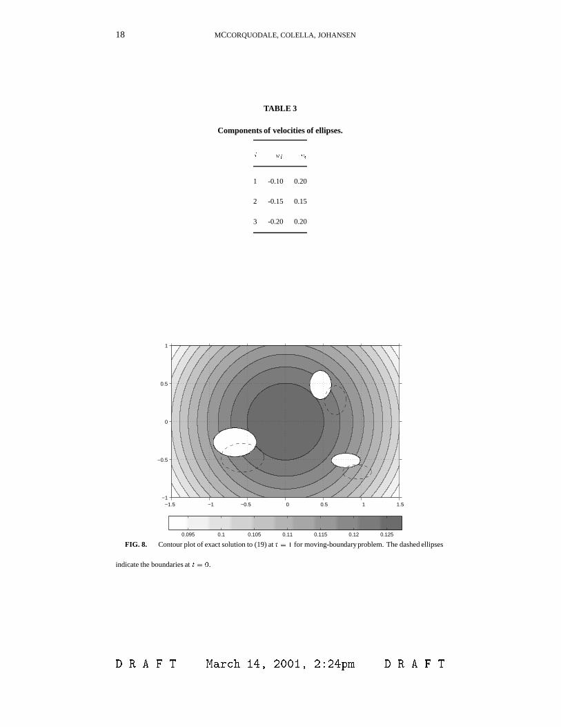
A contour plot of the exact solution to (19) at t = 1 is shown in Fig. 8.

Figure 9 shows both the max-norm and the 1-norm of the solution error at t = 1 for the

Dirichlet problem. Figure 10 shows the same quantities for the Neumann problem. We

see that when applied to these problems, the TGA method is second-order accurate in both

norms. The Crank–Nicolson is second-order accurate in 1-norm for the Neumann problem

but is zeroth-order in max norm, and diverges in both norms for the Dirichlet problem with

moving boundaries.

The solution error at t = 1 for the finest mesh spacing used (h = 180) in the TGA method

solving (19) is plotted in Fig. 11 for the Dirichlet problem and Fig. 12 for the Neumann

problem.

5. FUTURE WORK

The method described here, together with that in [6] for elliptic PDE’s and [8] for

hyperbolic PDE’s provide the fundamental components required for developing second-

order accurate methods for a broad range of continuum mechanics problems in irregular

geometries based on the predictor-corrector approach in [2]. Similar approaches based on

formally inconsistent discretizations at the irregular boundary have been used previously

and observed to be stable [1, 9], so we expect that the extension to the more accurate

D R A F T March 14, 2001, 2:24pm D R A F T

18 MCCORQUODALE, COLELLA, JOHANSEN

TABLE 3

Components of velocities of ellipses.

i ui vi

1 -0.10 0.20

2 -0.15 0.15

3 -0.20 0.20

0.095 0.1 0.105 0.11 0.115 0.12 0.125

−1.5 −1 −0.5 0 0.5 1 1.5 −1

−0.5

0

0.5

1

FIG. 8. Contour plot of exact solution to (19) at t = 1 for moving-boundaryproblem. The dashed ellipses

indicate the boundaries at t = 0.

D R A F T March 14, 2001, 2:24pm D R A F T

EMBEDDED BOUNDARY METHOD FOR THE HEAT EQUATION 19

10−2

10−1

10−8

10−7

10−6

10−5

10−4

10−3

10−2

r = 2

h

||ξ||∞

10−2

10−1

10−8

10−7

10−6

10−5

10−4

10−3

10−2

r = 2

h

||ξ||1

FIG. 9. Solution error at t = 1 in TGA method (circles) and Crank–Nicolson method (stars), with Dirichlet

conditions for (19) on moving boundaries. Left-hand plot shows max norm, right-hand plot shows 1-norm.

10−2

10−1

10−7

10−6

10−5

10−4

10−3

r = 2

h

||ξ||∞

10−2

10−1

10−7

10−6

10−5

10−4

10−3

r = 2

h

||ξ||1

FIG. 10. Solution error at t = 1 in TGA method (circles) and Crank–Nicolson (stars), with Neumann

conditions for (19) on moving boundaries. Left-hand plot shows max norm, right-hand plot shows 1-norm.

D R A F T March 14, 2001, 2:24pm D R A F T

20 MCCORQUODALE, COLELLA, JOHANSEN

0 0.5 1 1.5

x 10−7

−1.5 −1 −0.5 0 0.5 1 1.5 −1

−0.5

0

0.5

1

FIG. 11. Contour plot of absolute value of solution error to (19) at t = 1 for moving boundaries, Dirichlet

boundary conditions, h = 0:0125 in TGA method.

0 0.5 1 1.5 2 2.5 3 3.5 4 4.5

x 10−7

−1.5 −1 −0.5 0 0.5 1 1.5 −1

−0.5

0

0.5

1

FIG. 12. Contour plot of absolute value of solution error to (19) at t = 1 for moving boundaries, Neumann

boundary conditions, h = 0:0125 in TGA method.

D R A F T March 14, 2001, 2:24pm D R A F T

EMBEDDED BOUNDARY METHOD FOR THE HEAT EQUATION 21

boundary discretization should be straightforward. For embedded boundary methods to

be practical, it is necessary to use them in conjunction with block-structured adaptive

mesh refinement, particularly in three dimensions. This is routine for the case where

the embedded boundary is contained in the finest level of refinement [6], but requires

some additional discretization design when the embedded boundary crosses coarse-fine

interfaces.

One issue that has not been completely addressed is discrete conservation. For the

case of fixed boundaries, both the Crank–Nicolson and TGA algorithms are in discrete

conservation form, i.e., the divided difference in time of the old and new values can be

written as a difference of fluxes of the form (4). In that case, the difference in the volume-

weighted sums of the dependent variables over any discrete subdomain is equal to the sum

of fluxes across the boundaries of the subdomain. This is not the case for the moving

boundary algorithm, since the conversion of the moving-boundary problem to a sequence

of fixed-boundary problems does not satisfy the appropriate summation-by-parts identity.

One possible way to correct this problem is to compute an estimate of the failure to conserve

based on a space-time quadrature formula, which is used to construct a conservative and

stable increment of the solution that restores overall conservation, analogous to what is

done in the hyperbolic case [4, 3]. Such an approach was proposed in [7], but the modified

update triggered the boundary instability of the hybrid Crank–Nicolson method used there.

We expect that such a method would have no stability problems due to the L0 stability of

the TGA time discretization.

REFERENCES

1. A. S. Almgren, J. B. Bell, P. Colella, and T. Marthaler. A Cartesian mesh method for the incompressible Euler

equations in complex geometries. SIAM Journal on Scientific Computing, 142(1):1–46, May 1997.

2. J. B. Bell, P. Colella, and H. M. Glaz. A second order projection method for the incompressible Navier-Stokes

equations. J. Comput. Phys., 85(2):257–283, December 1989.

D R A F T March 14, 2001, 2:24pm D R A F T

22 MCCORQUODALE, COLELLA, JOHANSEN

3. J. B. Bell, P. Colella, and M. Welcome. A conservative front-tracking for inviscid compressible flow. In

Proceedings of the Tenth AIAA Computational Fluid Dynamics Conference, pages 814–822. AIAA, June

1991.

4. I.-L. Chern and P. Colella. A conservative front tracking method for hyperbolic conservation laws. Technical

Report UCRL-97200, Lawrence Livermore National Laboratory, July 1987.

5. N. Gilbarg and N. S. Trudinger. Elliptic Partial Differential Equations of Second Order. Springer-Verlag,

New York / Berlin, 1977.

6. H. Johansen and P. Colella. A Cartesian grid embedded boundary method for Poisson’s equation on irregular

domains. J. Comput. Phys., 147(2):60–85, December 1998.

7. Hans Svend Johansen. Cartesian Grid Embedded Boundary Methods for Elliptic and Parabolic Partial Dif-

ferential Equations on Irregular Domains. PhD thesis, Dept. of Mechanical Engineering, Univ. of California,

Berkeley, December 1997.

8. D Modiano and P. Colella. A higher-order embedded boundary method for time-dependent simulation of

hyperbolic conservation laws. In Proceedings of the FEDSM 00 - ASME Fluids Engineering Simulation

Meeting, Boston, MA, June 2000.

9. Richard B. Pember, Ann S. Almgren, William Y. Crutchfield, Louis H. Howell, John B. Bell, Phillip Colella,

and Vincent E. Beckner. An embedded boundary method for the modeling of unsteady combustion in an

industrial gas-fired furnace. Technical Report UCRL-JC-122177, LLNL, October 1995. Presented at the 1995

Fall Meeting of the Western States Section of the Combustion Institute – Stanford University.

10. E. H. Twizell, A. B. Gumel, and M. A. Arigu. Second-order, L0-stable methods for the heat equation with

time-dependent boundary conditions. Advances in Computational Mathematics, 6(3):333–352, 1996.

D R A F T March 14, 2001, 2:24pm D R A F T