A Method for Computing the PartialDerivatives of Experimental Data

Y. Leong Yeow, Jordan Isac, and Fathullah A. KhalidDept. of Chemical and Biomolecular Engineering, The University of Melbourne, Parkville, VIC 3010, Australia

Yee-Kwong LeongDept. of Mechanical Engineering, University of Western Australia, Crawley, WA 6009, Australia

A. S. LubanskyDept. of Engineering Science, University of Oxford, Oxford OX1 3PJ, U.K.

DOI 10.1002/aic.12236Published online April 5, 2010 in Wiley Online Library (wileyonlinelibrary.com).

This article describes a procedure for obtaining the partial derivatives of experimen-tal data that depend on two independent variables. The starting equation is an ill-posed integral equation of the first kind. Tikhonov regularization is used to keep noiseamplification under control. Implementation of the computation steps is described andthe performance of the procedure is demonstrated by four practical examples. VVC 2010

American Institute of Chemical Engineers AIChE J, 56: 3212–3224, 2010

Keywords: partial derivative, integral equation, inverse problem, Tikhonovregularization, data interpolation

Introduction

Scientific and engineering investigations often require theevaluation of the derivatives of experimental data. Comput-ing derivatives by any of the commonly adopted techniques,such as finite difference approximation or analytical differen-tiation of globally or locally fitted functions, is unlikely tolead to reliable results. This is because differentiation is aninherently ill-posed inverse problem. The unavoidable noisein the data will be amplified during the computation of thederivatives.1 Tikhonov regularization is a specialized tech-nique for handling ill-posed inverse problems. Lubanskyet al.2 applied this technique to evaluate the ordinary deriva-tives of experimental data that depend on a single inde-pendent variable. The built-in regularization parameter inTikhonov regularization is able to keep noise amplificationunder control. This technique also has the advantage that itdoes not require the functional relationship between the de-pendent and independent variables to be known or specified.

The present article describes a procedure for obtaining thepartial derivatives of experimental data when the dependentvariable is a function of two independent ones. Examples ofsuch data include variation of the volume percent of anagglomerating suspension with floc size and time, the de-pendence of specific volume of a binary solution on compo-sition and temperature, the change in the pressure of a fluidwith density and temperature. The procedure to be developedalso relies on Tikhonov regularization to keep noise amplifi-cation under control but starts from a governing equationthat is entirely different from that used by Lubansky et al. Italso involves significantly different computation steps whichare considerably more complicated.

For the purpose of describing the development of the newprocedure, the two independent variables will be denotedgenerally by x and y and the dependent variable by z, i.e.,z ¼ f(x, y). Apart from the general requirement that f(x, y)be a well-behaved function that can be differentiated asmany times as required this new procedure again does notrequire its functional form to be known or specified.

The input to the procedure is a set of experimental data inthe general form {[xM1 , y

M1 , z

M1 ]

T, [xM2 , yM2 , z

M2 ]

T, … [xMi , yMi ,

zMi ]T, … [xND

M, yND

M, zND

M]T}. The superscript M is used here to

Correspondence concerning this article should be addressed to Y. L. Yeow atyly@unimelb.edu.au.

VVC 2010 American Institute of Chemical Engineers

3212 AIChE JournalDecember 2010 Vol. 56, No. 12

THERMODYNAMICS

distinguish experimentally determined quantities from theircomputed counterparts, which will carry a superscript C. ND

is the number of points in the data set. These data points arearranged in ascending order of the independent variables(x, y). It is assumed that all the measurement points fallwithin the rectangle, the measurement rectangle, with (xref,yref) as its lower left corner and the last measurement point(xND

yND) as its upper right corner. The coordinates (xref, yref)

of the lower left corner, referred to as the reference point, isgiven by (Min[xi], Min[yi]), i ¼ 1 to ND. See Figure 1. Inmost cases (xref, yref) is also the first data point (x1, y1) ofthe data set. In all the subsequent computation, the experi-mental data will be normalized using the following scalingfactors (xND

� xref), (yND� yref) and (Max[zi] � Min[zi]), i

¼ 1 to ND in the x-, y-, and z-direction, respectively.The introduction of a second independent variable brings

with it a number of complications. The most obvious one isthat there are now two first partial derivatives, (qz/qx)y and(qz/qy)x, to be evaluated instead of just a single ordinary de-rivative dz/dx. This not only increases the computing loadsignificantly but also the mathematical complexity of theproblem compared to that for ordinary derivative. In the sub-sequent paragraphs, the two partial derivatives will bedenoted by p(x, y) : (qz/qx)y and q(x, y) : (qz/qy)x Thesubscript showing which independent variable is being heldfixed will be suppressed when that does not lead to confu-sion.

As general functions p(x, y) and q(x, y) are independent ofone another. However, the mixed second derivatives of awell-behaved f(x, y) satisfy the relationship q((qz/qx)y/qy)x ¼q((qz/qy)x/qx)y.

3 This gives rise to an equation relating p(x,

y) and q(x, y) that has no counterpart when evaluating ordi-nary derivatives

ð@p=@yÞx ¼ @ðð@z=@xÞy=@yÞx ¼ @ðð@z=@yÞx=@xÞy ¼ ð@q=@xÞy:(1)

This condition has to be met even in practical situationswhere the physical interest is only in the first derivativesp(x, y) and q(x, y) and represents an added complication inthe partial derivative problem.

In typical a experiment measurements may not be carriedout at regularly spaced out independent variables (x, y) andconsequently the measurement points (xi, yi), i ¼ 1 to ND canbe irregularly distributed within the measurement rectangle.This adds to the complication in the representation of the datapoints and of the partial derivatives p(x, y) and q(x, y) at thesepoints within the two-dimensional discretized measurementrectangle with all the attendant added computing overhead.

The governing equation and its discretization together withthe computation steps of the new procedure will be describedin the next section. This is followed by a section in which aseries of examples are introduced to demonstrate the new pro-cedure in action. These examples, apart from their practicalinterest, have been selected so that the partial derivatives gen-erated by Tikhonov regularization can be checked againstresults obtained independently by other methods.

Governing Equation, Discretization, andImplementation

The line integral equation

The value of the dependent variable zi at a general mea-surement point (xi, yi) is related to the partial derivativesp(x, y) and q(x, y) along the linear path l joining the refer-ence point (xref, yref) to the general point (xi, yi) by the lineintegral

zCi ¼Zðxi;yiÞ

ðxref ;yref Þ

rzðx0; y0Þ:dlþ zCref ¼Zðxi;yiÞ

ðxref ;yrefÞ

pðx0; y0 Þdx0

þZðxi;yiÞ

ðxref ;yrefÞ

qðx0; y0 Þ dy0þzCref for i ¼ 1; 2;…ND: ð2Þ

zCi is the computed equivalent of the measured quantity zMi andzCref is the computed value of z at (xref, yref). (x

0, y0) that appearwithin the integrals are dummy variables representing ageneral point on the linear path l. Equation 2 can be regardedas an integral equation of the first kind to be solved, togetherwith Eq. 1, for the unknown functions p(x, y) and q(x, y) andthe unknown constant zCref so that the computed and measuredvariables are in agreement. This equation is very differentfrom the governing equation, based on a two-term Taylorseries with integral-form remainder term, used by Lubanskyet al.2 in the ordinary derivative problem.

Discretized equations

For the purpose of formulating the computation steps, it isconvenient to put the experimental data in the form of a

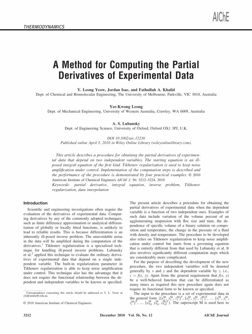
Figure 1. Representation of the derivatives at the inter-section points (~) of the integration path ( )with gridlines and at the measurement point(n) by that at the nearest grid points (l).

The integration path connects the reference point (n) at thelower left corner, on the boundary (— — —), of the mea-surement rectangle to the measurement point. Pa, Pc, andPm are represented by the linear interpolation of (Pa1 andPa2), (Pc1 and Pc2), and (Pm1, Pm2, Pm3, and Pm4),respectively.

AIChE Journal December 2010 Vol. 56, No. 12 Published on behalf of the AIChE DOI 10.1002/aic 3213

known column vector: zM ¼ [zM1 , zM2 , … zMi , … zND

M]T and a

known matrix with two columns: [xM, yM] ¼ [(xM1 , yM1 ), (x

M2 ,

yM2 ), (xMi , y

Mi ), … (xND

M, yND

M)]T. The dimensionless measure-

ment rectangle is discretized into NT ¼ NK � NK two-dimen-

sional uniformly spaced grid points. To ensure accurate rep-

resentation of the measured data, NT is usually set to be

much larger than ND. In all the examples below, NK ¼ 41

and NT ¼ 41 � 41 ¼ 1681. The uniform discretization grid

spacing will be denoted by D and the coordinates of the

dimensionless discretization grid points by column vectors

xC ¼ [xC1 ¼ 0, xC2 , … xCj ,…xNT

C ¼ 1]T, yC ¼ [yC1 ¼ 0,

yC2 ,…yCj ,…yNT

C ¼ 1]T to distinguish them from the measure-

ment points [xM, yM]. In general, these two sets of coordi-

nate points do not coincide.The numerical value of the unknown derivatives p(x, y)

and q(x, y) at each of the discretization grid points will be

denoted by the unknown column vectors p ¼ [p1, p2,…pj,..pNT

]T and q ¼ [q1, q2, qj,..qNT]T. In terms of these discre-

tized variables, Eq. 2 takes the form

zCi ¼XNT

j¼1

Aijpj þXNT

j¼1

Bijqj þ zCref for i ¼ 1; 2;…ND (3)

or in matrix notation

zC ¼ Apþ Bqþ 1zCref ¼ A B 1½ �p

q

zCref

264

375 ¼ CP : (4)

From Eq. 3 it is clear that A and B are ND � NT matri-

ces of known numerical coefficients arising from the

approximation of the integrals in Eq. 2 by the trapezoidal

rule. To arrive at these coefficients, the derivatives p(x0, y0)and q(x0, y0) at any intersection point of the linear path l

with the discretization gridlines are expressed, by linear

interpolation, in terms of the elements of p and of q closest

to that point. See Figure 1. For a typical measurement point

(xMi , yMi ) that does not coincide with a grid point its p(xMi ,

yMi ) and q(xMi , yMi ) are again given by a linear combination

of the appropriate elements of the p and q column vectors.

1 in Eq. 4 is a column vector with ND elements each equal

to unity.

In the final form of Eq. 4, to simplify the computation

steps, the unknown column vectors p and q and the

unknown constant zCref are treated as a single column vector

with (2NT þ 1) unknown elements and denoted by P ¼[p1, p2,…pj,..pNT

, q1, q2,…qj,..qNT, zCref]

T. C is the ND � (2NT

þ 1) matrix formed by the concatenation of the matrices A

and B and 1 to reflect the introduction of the combined

unknown column vector P.

A and B and, hence, C are sparse matrices. For example,in the ith row of A and B only those elements associatedwith the pj and qj of those discretization points that lie im-mediately next to the integration path are non zero with allthe other elements being identically zero. The numericalvalue of the non-zero elements are, as explained above,given by linear interpolation, i.e., inversely proportional totheir distances from the intersection point. The locations of

these non-zero elements in C depend on how the NT girdpoints are ordered and numbered.

Discretization of Eq. 1 leads to a finite difference equationof the form

pjþ � pj�

2D� qjþ � qj�

2D¼ 0; (5)

for each and every interior discretization point (xj, yj). Thereare thus (NK � 2) � (NK � 2) of Eq. 5 to be met. Simplecentral difference has been used to approximate the first partialderivatives (qp/qy)x and (qq/qx)y. pjþand pj� in Eq. 5 represent,in shorthand notation, the x partial derivative (qz/qx)y at thetwo immediate neighboring points (xj, yj þ D) and (xj, yj � D)of (xj, yj). Similarly, qjþand qj�denote the y partial derivative(qz/qy)z at the neighboring points (xj þ D, yj) and (xj � D, yj).When assembled, the (NK � 2) � (NK � 2) of Eq. 5 take thefollowing form:

DP ¼ 0: (6)

The number zeros in the null column vector 0 and thenumber of rows in D are both equal to (NK � 2) � (NK �2) corresponding to the number of internal points in themeasurement rectangle. The number of columns in D is 2NT

þ 1, i.e., the total number of unknowns in the column vectorP. In each row of D, according to the coefficients of Eq. 5,there are only four non-zero elements of either 1 or �1 withall the remaining elements being identically zero. The loca-tions of the non-zero elements in D again depend the waythe NT grid points are numbered.

The unknowns P1, P2, P3, ..... P2NTþ1 are required to mini-mize the following sums of squares

(1) S1 ¼ [zC � zM]T[zC � zM];(2) S2 ¼ [DP]T[DP];(3) S3 ¼ Sum of squares of q2p(x, y)/qx2, q2q(x, y)/qx2,

q2p(x, y)/qy2, and q2q(x, y)/qy2 at the (NK � 2) � (NK � 2)interior discretization points together with that of q2p(x, y)/qy2 and q2q(x, y)/qy2 at the 2(NK � 2) interior points of thetwo x-constant boundaries and that of q2p(x, y)/qx2 andq2q(x, y)/qx2 at the 2(NK � 2) interior points of the two y-constant boundaries.

Condition (1) ensures that the zC at the measurement points

(xM, yM) approximates zM closely at the measurement points.

This is the same as that imposed by Lubansky et al. in their

computation of ordinary derivatives. Condition (2) enforces

the equality of the two mixed second derivatives of z ¼ f(x,y). This has no equivalent in the ordinary derivative problem.

Condition (3), following the general practice in Tikhonov reg-

ularization, ensures that the computed p(x, y) and q(x, y) do

not show spurious fluctuations. Condition (3) together with

the assumed well-behaved nature of f(x, y) ensures that the

sum of squares of the mixed second derivatives of p(x, y) andq(x, y) are also minimized. The total number of second deriv-

atives involved in Condition (3) is thus 4(NK � 2) � (NK �2) þ 2[2 � 2 (NK � 2)] ¼ 4NK (NK � 2).

It is necessary to restrict Conditions (2) and (3) to the in-terior points so that all the second derivatives of p(x, y) andq(x, y) that appear in them can be approximated by the finite

3214 DOI 10.1002/aic Published on behalf of the AIChE December 2010 Vol. 56, No. 12 AIChE Journal

difference of the elements of the unknown column vector P.This avoids the necessity of including in P additionalunknowns associated with grid points outside of the mea-surement rectangle.

Tikhonov regularization

In Tikhonov regularization, instead of minimizing (1), (2),and (3) separately, their linear combination R ¼ S1 þ S2 þkS3 is minimized.1 k is the regularization parameter that bal-ances the two separate requirements. A large k favors thesmoothness condition while a small k favors the accuracycondition and the equality of the mixed second derivativesof f(x, y). The appropriate choice of k depends on ND andNK and also on the noise level in the data and is not a physi-cal property of the f(x, y). It is, therefore, not useful, in factmay be confusing, to report the numerical value of k used inthe examples below. In this investigation, the choice of k isguided by the simple and practical expectation that the aver-age deviation of zC from zM(x, y) at the measurement pointsis of the same order of magnitude as the expectedexperimental error bar of zM. This is often referred to as theMorozov Principle1 in mathematical texts.

For any k, the unknowns P ¼ [P1, P2, P3, ... P2NTþ1] thatminimize R are given by1

P ¼ ½ETEþ kbTb��1ETZM

ext: (7)

The composite matrix E and the extended column vec-tor ZM

ext are formed, respectively, by the joining of thematrices C and D in Eqs. 4 and 6 and of the knowncolumn vectors zM and the null column vector 0 on theRHS of Eq. 6.

E ¼ C

D

� �and ZM

ext ¼ zM

0

� �: (8)

The matrix b in Eq. 7 arises from the use of standard cen-tral finite difference to approximate the second derivativesq2p/qx2, q2p/qy2, q2q/qx2, and q2q/qy2 at each interior gridpoint of the measurement rectangle and selected members ofthese second derivatives at the interior points on the fourboundaries. Each row of b has only three non-zero elementsgiven by 1, �2, and 1 with all other elements being identi-cally zero. As in the C and D, the locations of the non-zeroelements depend on NK and on the way the total set of NT

discretization points are numbered. Each row of b is termi-nated by an extra zero to allow for the incorporation of zCrefinto P. This is because zCref plays no role in the approxima-tion of the second derivatives of p(x, y) and q(x, y). Thus, bhas 4NK � (NK � 2) rows and (2NT þ 1) columns.

Equation 7 is the linear algebraic equation that convertsthe experimental data z

M into the partial derivatives (qz/qx)yand (qz/qy)x at a set of closely and regularly spaced discreti-zation points. These partial derivatives allow the dependentvariable at the measurement points z

C to be calculated withrelative ease

zC ¼ CP: (9)

Comparison of zC with z

M provides an instant check onthe partial derivatives. These partial derivatives can also besubstituted into Eq. 2 and the two integrations performednumerically to back calculate the dependent variable zC atany point of the measurement rectangle.

Applications and Results

Synthetic data

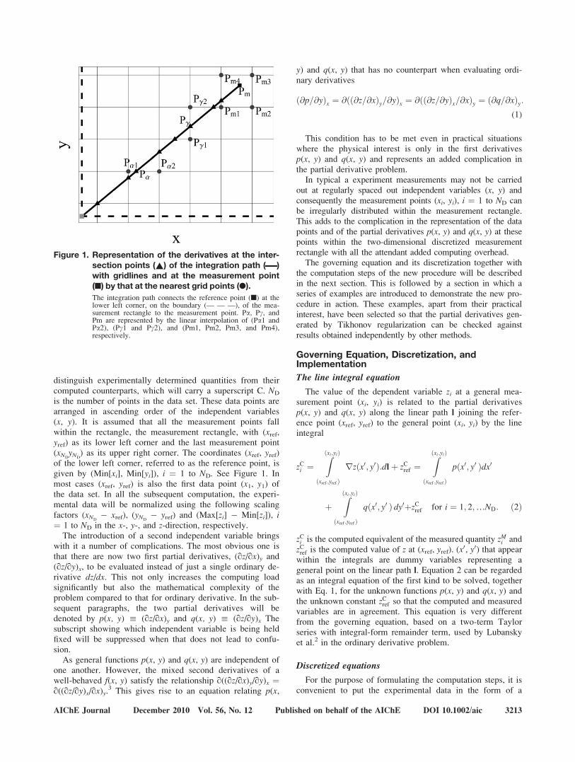
The discrete points in Figure 2a were generated by thewell-behaved function f(x, y) ¼ cos(x2)cosh(y) with the mea-surement points [xM, yM] shown in Figure 2b. These mea-surement points, ND ¼ 121, are irregularly distributed within

Figure 2. Synthetic data and measurement points.

(a) Exact data points based on z ¼ cos(x2) cosh(y). (b) Irregularly distributed measurement points.

AIChE Journal December 2010 Vol. 56, No. 12 Published on behalf of the AIChE DOI 10.1002/aic 3215

the square defined by (0, 0) and (1, 1). The generating func-tion f(x, y) allows the computed partial derivatives to becompared directly against their exact analytical counterparts.

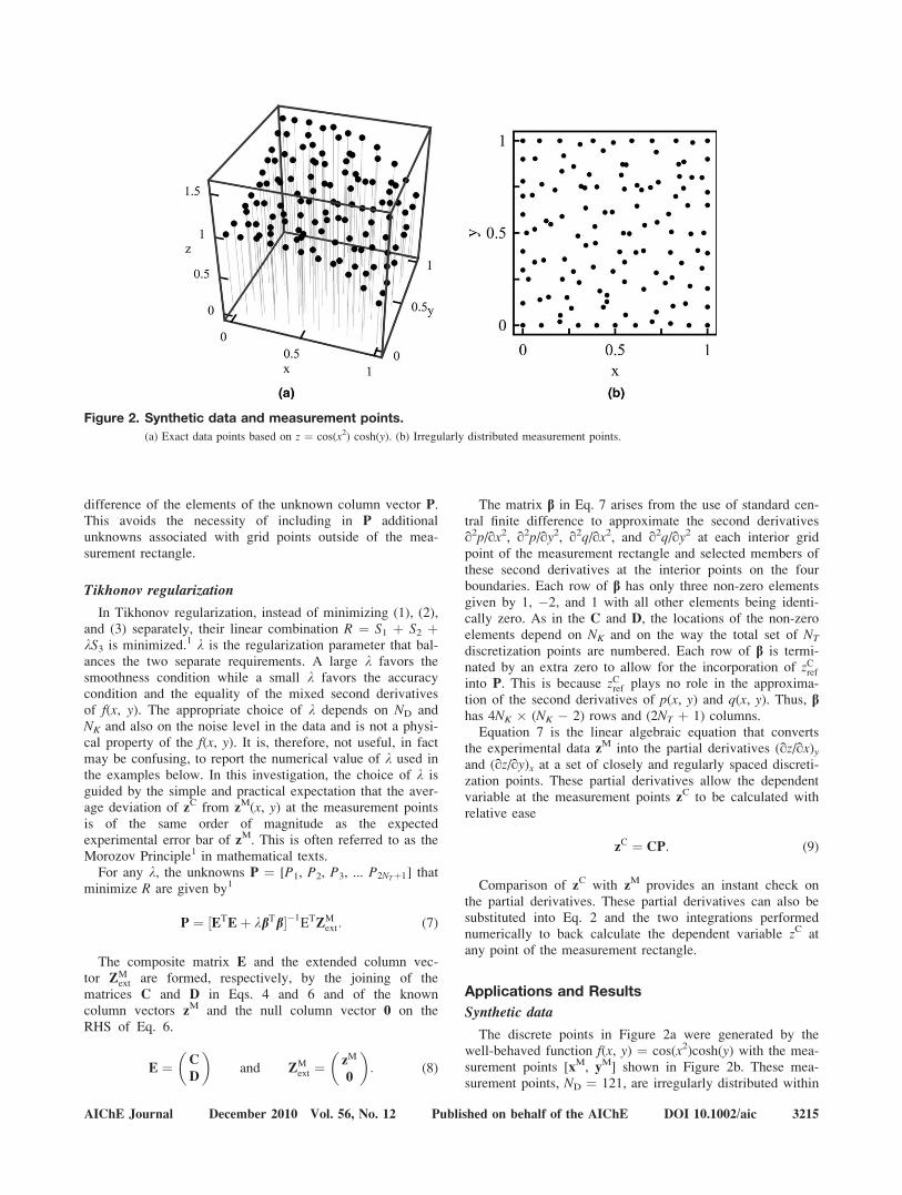
The computed partial derivatives generated by Eq. 7 areshown as a continuous surface in Figures 3a, b. These surfa-ces are visually indistinguishable from the surfaces given bythe exact partial derivatives (not shown). For a more quanti-tative comparison, the computed partial derivatives areshown as continuous curves in Figures 3c, d. x appears as aparameter in (c) and y as a parameter in (d). The large NT

allows the computed partial derivatives at the discretizationpoints to be treated essentially as continuous curves. Thecorresponding curves based on the exact partial derivativesare shown as lighter broken curves on the same plot. Thecomputed results agree with the exact partial derivatives tobetter than 0.01%. This is not very surprising as there is noerror in the synthetic data and the function z ¼ f(x, y) usedin this case is a relatively simple function with no localmaxima or minima.

To test the performance of Eq. 7 in the presence ofunavoidable measurement noise, �1% random noise is now

added to the data points in Figure 2a. The computed partialderivatives based on these ‘‘noisy’’ data are shown in Fig-ures 4a, b as continuous curves. The broken curves areagain the exact results. An immediate consequence of theadded noise is that a much larger regularization parameterk, compared to that in the earlier computation, is needed tosuppress fluctuations in the partial derivatives. As expected,the deviation from the exact partial derivatives hasincreased. The average deviation of the two partial deriva-tives is significantly [10%. This deviation becomes particu-larly large close to the boundaries of the measurementregion. However, for many practical purposes, these com-puted results remain acceptable. It is interesting to note thatthe zC (not shown) backed calculated from these partialderivatives is still in very good agreement with the exactfunction with an average deviation \0.1% indicating thatthe back-calculated zC as a function of dependent variablesx and y can be used to interpolate or to smooth the noisydata. The greatly amplified deviation observed in the com-puted partial derivatives is a manifestation of the ill-posednature of the problem.

Figure 3. Computed and exact partial derivatives.

(a) Computed surface of (qz/qx)y; (b) Computed surface of (qz/qy)x; (c) Comparison of computed (qz/qx)y ( ) against exact (qz/qx)y ( )at constant x. x ¼ 0 (the top most curve), 0.25, 0.5, 0.75, and 1 (the lowest curve); (d) Comparison (qz/qy)x ( ) with exact (qz/qy)x ( )at constant y. y ¼ 0 (the lowest curve), 0.25, 0.5, 0.75, and 1 (the top most curve).

3216 DOI 10.1002/aic Published on behalf of the AIChE December 2010 Vol. 56, No. 12 AIChE Journal

Particle size distribution in yeast cells agglomeration

Particle size distribution (PSD) is a key operation variablein particulate processes such as crystallization, suspensionflocculation, and cell agglomeration. It shows the relation-ship between vol % and floc size L and how this changeswith time t. Thus, a typical PSD takes the form of a function

of two independent variables / ¼ f(t, L). For any t, d/ ¼f(t, L)dL gives the proportion of particles with size betweenL � dL/2 \ L \ L þ dL/2. f(t, L) is assumed to be a well-behaved function of t and L. (q//qt)L gives the rate ofgrowth of the proportion with size L while (q//qL)t is ameasure of its instantaneous variation with L. These partialderivatives are of practical interest and appear explicitly inthe general population-balance equation used to describe par-ticulate processes.4 In this example, Eq. 7 will be used toobtain these partial derivatives based on a small set of exper-imental /(t, L) data for cell agglomeration.

Han et al.5 investigated the effects of different flocculants

and their dosage on the agglomeration of yeast cells. Using

a laser diffraction particle size analyzer, they monitored the

vol % as a function of floc size, between 1 lm and 450 lm,

of a yeast cell suspension during the agglomeration process.

They recorded the PSD at regular intervals for an agglomer-

ation time of over 10 min. A subset, 180 s � t � 642 s and

28.25 lm � L � 295.83 lm, of their large data collection

will be used in this example. These are plotted, as discrete

points, against floc size L, in Figure 5. There are 20 separate

PSD data sets in these plots. The measurement time, fixed

on a PSD, increases variously by 21 s to 42 s between sets.

For each PSD, the particle size analyzer gives the vol % at

the same 18 preselected floc sizes. ND ¼ 360 in this com-

bined PSD data sets. For visual clarity, the PSD data points

for consecutive measurement times are spread out on differ-

ent plots.

The partial derivatives (q//qt)L and (q//qL)t given by

Eq. 7 are shown in Figures 6a, b. k has been adjusted to

eliminate excessive fluctuations. These partial derivatives

were substituted in Eq. 2 and the back-calculated /C(t, L)are shown as continuous curves in Figure 5. The curves are

in reasonable agreement with the experimental data with an

average deviation of around 8.2%. The deviation close to the

boundaries of the measurement rectangle is again larger than

that in the interior of the rectangle.As a more direct check on the computed (q//qt)L and

(q//qL)t, the /M data points for a fixed t is treated as a func-

tion of L and that for a fixed L as a function of t. The Tikho-

nov regularization procedure of Lubansky et al. for data of a

single dependent variable is now used to compute the ordi-

nary derivatives d//dt and d//dL. These ordinary derivatives

are compared against the corresponding partial derivatives.

Typical examples of such comparison are shown in Figures

6c, d. The partial derivatives and the corresponding ordinary

derivatives are shown as continuous and lighter broken

curves, respectively. Although the general trends of the par-

tial and ordinary derivatives are in reasonable agreement,

there are significant differences between them particularly

near the boundaries of the measurement region. In view of

the noise in the data, the differences in the two computation

schemes and the large number of computing steps involved

the observed level of agreement is considered as acceptable.

Another possible contributory factor to the differences is the

relatively small number of points, ND ¼ 18 in the constant tdata and ND ¼ 20 in the constant L data, used in the compu-

tation of the ordinary derivatives compared to 360 used in

the partial derivatives computation.

Figure 4. Computed derivatives based on noisy dataand exact derivatives.

(a) Comparison of computed (qz/qx)y ( ) with exact (qz/qx)y ( ) at constant x. x ¼ 0 (the top most curve), 0.25, 0.5,0.75, and 1 (the lowest curve); (b) Comparison (qz/qy)x ( )with exact (qz/qy)x ( ) at constant y. y ¼ 0 (the lowest curve),0.25, 0.5, 0.75, and 1 (the top most curve).

AIChE Journal December 2010 Vol. 56, No. 12 Published on behalf of the AIChE DOI 10.1002/aic 3217

Partial molar volume of MIPA

Mokraoui et al.6 measured the density of aqueous monoi-sopropanolamine (MIPA) solutions with different mole frac-tion xW of water. They reported the density data for a seriesof constant temperature T between 273.15 K and 353.15 K.Their raw data have been converted into specific volume vand shown in Figure 7a as a function of the two independentvariables T and xW, i.e., v ¼ f(T, xW). The data points in thisplot, ND ¼ 345, lie on a featureless near-to-flat surface.

The partial derivatives ð@v=@TÞxW and ð@v=@xWÞT , treatedas a function of T and xW, obtained by Tikhonov regulariza-tion are shown in Figures 7b, c. As expected, ð@v=@TÞxW isrelatively small and the surface, apart from the trend ofdeveloping a small local maximum at low temperature, isquite featureless. ð@v=@xWÞT is significantly larger and atlow temperature shows a clear local maximum in the neigh-borhood of xW ¼ 0.8. Apart from the slight ripples at theboundaries of the measurement region, the surfaces of thepartial derivatives appear to be well behaved.

ð@v=@TÞxW and ð@v=@mWÞT by themselves are not of par-ticular physical interest but they are essential for the compu-tation of the partial molar volumes VW and VMIPA. At anytemperature, these two thermodynamic variables are relatedto the partial derivative (qv/qxW)T by7

VMIPAðT; xWÞ ¼ v� xW@v

@xW

� �T

; VWðT; xWÞ

¼ vþ ð1� xWÞ @v

@xW

� �T

: ð10Þ

In these expressions, the specific volume v(T, xW), for anypoint in the measurement rectangle, is obtained by substitutingthe partial derivatives into Eq. 2 and performing line integralnumerically. The resulting partial molar volume surfaces areshown in Figure 8a. They exhibit a local minimum or maxi-mum in the neighborhood of xw ¼ 0.8 for some T. These are inagreement with the restricted partial molar volumes reported byMokaroui et al.6 and of Yeow et al.8 In their computation, theseauthors treated the specific volume data at each measurementtemperature as a function of single independent variable, i.e.,v ¼ f(xW) and obtained the ordinary derivative dv/dxW from fit-ted expression6 and from Tikhonov regularization computa-tion,8 respectively. They then used the ordinary derivative tocompute the partial molar volumes at each of the measurementtemperatures. A comparison of the partial volumes, as generalfunctions of T and xW, obtained in this investigation with those,as functions of xw at the discrete measurement temperatures,obtained in the two earlier investigations is shown in Figure 8b.These plots show the partial molar volumes at T ¼ 353.15,283.15, 318.15K and, i.e., the highest, lowest measurementtemperatures and their average. The continuous curves are theresults from Eq. 7, the lighter broken curves are from Yeowet al.8 and the discrete points are from Mokaroui et al.6 Theagreement among these results is indicative of the reliability ofthe partial derivatives in Figure 7b.

T-q-P data of supercritical methane

Trappeniers et al.9 reported the pressure P of supercriticalmethane as a function of temperature T (between 273.16 and423.16 K) and density q (between 13.23 and 410.91 kg

Figure 5. Experimental and computed PSD of yeast cells.

Discrete points are the experimental data of Han et al.5 and continuous curves are back calculated from the partial derivatives given by Eq.7. Upper row left to right: t ¼ 180 (n), 284 ( ), 389 (^), 494 (l) s; t ¼ 201 (n), 305 ( ), 410 (^), 515 ( ) s; t ¼ 222 (n), 326 ( ),431 (^), 557 ( ) s. Lower row left and right: t ¼ 243 (n), 347 ( ), 452 (^), 600 ( ) s; t ¼ 263 (n), 368 ( ), 473 (^), 642 ( ) s.

3218 DOI 10.1002/aic Published on behalf of the AIChE December 2010 Vol. 56, No. 12 AIChE Journal

m�3). Their data are shown as discrete points in Figure 9aand enlarged in Figure 9b for low q. In the present computa-tion, those data points with q [ 269.14 kg m�3 in the origi-nal data set of Trappeniers et al. have been left out andnot shown in Figures 9a, b as these measurements do notcover the entire temperature range. ND ¼ 408 for thisreduced T-q-P data set.

Adopting the same approach as in the previous examples,Eq. 7 was applied to compute the partial derivatives (qP/qT)q and (qP/qq)T for the measurement rectangle defined byTmin ¼ 273.16 K � T � Tmax ¼ 423.16 K and qmin ¼ 13.23kg m�3 � q � 269.14 kg m�3 ¼ qmax. Typical plots of

these partial derivatives are shown as continuous curves inFigures 9c, d. The curves in Figure 9c are for Tmin, (Tmax þTmin)/2, and Tmax. Those in Figure 9d are for qmin, (qmax þqmin)/2, and qmax. The computed partial derivatives over theregion measurement rectangle have been substituted into Eq.2 and integrated numerically to give the pressure P. Thisback-calculated P is shown in Figures 9a, b as continuouscurves. The average difference between the back-calculatedP and the experimental data is about 0.3%, which is thesame order of magnitude as the error bars of the experimen-tal data. However, it can be seen that at low q there is veryperceptible deterioration in agreement.

Figure 6. Computed derivatives of /.

(a) Computed (q//qt)L in vol % (lm)�1 s�1; (b) Computed (q//qL)t in vol % (lm)�2; (c) Comparison of (q//qt)L ( ) and d//dt ( ),L ¼ 28.25, 74.31, 295.83 (left to right) lm; (d) Comparison of (q//qL)t ( ) and d//dL ( ), t ¼ 180, 368, and 642 (left to right) s.

AIChE Journal December 2010 Vol. 56, No. 12 Published on behalf of the AIChE DOI 10.1002/aic 3219

Setzmann and Wagner10 have developed a single expres-sion capable of representing a large number of the thermody-namic properties of methane. These properties include en-

thalpy, entropy, specific heat under different conditions, ther-mal expansion coefficient, compressibility, Joule-Thomsoncoefficient, isothermal expansion coefficient as well as pres-sure P over a very wide range of T and q. Their expression,adopted by IUPAC, consists of two series each with a largenumber of terms. The large number of parameters, well over180, associated with these series were determined by least-squares fitting of the expression to a very large collection ofthermodynamic properties taken from the literature. Their nu-merical values are tabulated in Setzmann and Wagner10 andwill not be repeated here. The resulting expression that givesP in terms of T and q has been differentiated with respect tothe independent variables to yield (qP/qT)q and (qP/qq)T. Thepartial derivatives generated this way are shown as light bro-ken curves in Figures 9c, d. Apart from the boundary of theregion analyzed, there is a very satisfactory agreementbetween the two sets of curves in each plot verifying the reli-ability of the results of Tikhonov regularization computation.

The isobaric partial derivative (qq/qT)P of fluids is ofpractical interest and appears explicitly in a number of ther-modynamic identities. This partial derivative is related to thetwo partial derivatives of P, i.e., (qP/qT)q and (qP/qq)T bythe standard mathematical relationship3

ð@q=@TÞP ¼ �ð@P=@TÞq=ð@P=@qÞT (11)

The partial derivatives of methane generated by Eq. 7 aresubstituted into this equation and the resulting (qq/qT)P isplotted against q and shown as continuous curves in Figure10a for T ¼ Tmax, Tmin, and (Tmax þ Tmin)/2. The computed(qq/qT)P is also plotted against T for q ¼ qmin and qmax aswell as a number of in between q. For comparison, the cor-responding results obtained from the general expression ofSetzmann and Wagner are again shown as broken curves onthese plots. The agreement while satisfactory in general isshowing signs of deterioration close to the boundaries of themeasurement region. The deterioration is most significantfor q close to qmin and qmax as can be observed from thecurves for q ¼ qmin and qmax in Figure 10b. This is under-standable as the error in the two partial derivatives (qP/qT)qand (qP/qq)T is amplified while applying Eq. 11.

Isothermal throttling coefficient w : (qh/qP)T is a ther-modynamic function of some practical importance. w whichrelates the change in specific enthalpy with pressure underisothermal condition can be measured directly in, for exam-ple, a flow calorimeter operating under isothermal mode.Through standard thermodynamic identities, it can be shownthat w is given by

w � ð@h=@PÞT ¼ ½1þ ðT=qÞð@q=@TÞP�=q: (12)

Thus, provided (qq/qT)P can be evaluated reliably, Eq. 12provides a means of obtaining w from experimental T-q-Pdata. The (qq/qT)P from Eq. 11 and the back-calculated qshown in Figure 9 are now used in conjunction with thisequation to obtain w. The outcome is plotted against T andshown as continuous curves in Figure 11a. On each of thesecurves, q is held fixed, between 50 and 250 kg m�3. w canalso be obtained from the general expression of Setzmannand Wagner. For comparison, this w is shown in Figure 11a

Figure 7. Properties of aqueous MIPA.

(a) Experimental v (cm3 mol�1) of Mokraoui et al.; (b)Computed surfaces of (b1) ð@v=@TÞxW (cm3 mol�1 K�1) and(b2) (qv/qxW)T (cm3 mol�1).

3220 DOI 10.1002/aic Published on behalf of the AIChE December 2010 Vol. 56, No. 12 AIChE Journal

as light broken curves. There is a very satisfactory agree-ment between the two sets of w over the range of T and qshown in this plot. However, for qmin \ q \ 50 kg m�3

(not shown) there is very significant difference. The differ-ence can be seen by plotting w as a function against q withT as an independent parameter. See Figure 11b. It is quiteclear that, for qmin \ q \ 50 kg m�3, the results based onthe results of Tikhonov regularization are erroneous. Thisfailure can be traced to the poor performance of the back-calculated q close to qmin, see Figure 9b, and also to theaccumulated error in (qq/qT)P, which is further amplified bythe small numerical value of q in this region.

Discussion

The derivation of Eq. 7 involves a sequence of steps thatmay appear complicated. But all of the steps involved are

relatively direct and intuitively obvious. For example, thegrouping of the unknowns into P and the combining ofthe matrices of coefficients to form composite matrices C

and E may appear convoluted but the resulting simplificationin the formulation and in the solution processes leadingto Eq. 7 is self evident. Furthermore, all the matrix mani-pulation steps leading to and in Eq. 7 can be handled auto-matically by scientific computing software with symbolicmanipulation capability requiring little or no physical inter-vention.

Experience shows that the setting up of the matrices A

and B in Eq. 4, D in Eq. 6, and b in Eq. 7 require someplanning. All these are sparse or very sparse matrices. As al-ready mentioned, the locations of the non-zero elements inthem depend on the way the discretization points in the two-dimensional grid are numbered. Computer-assisted bookkeeping of the immediate neighbors of a general grid point

Figure 8. Partial molar volumes of aqueous MIPA.

(a) Surfaces of VW and VMIPA (cm3 mol�1); (b) Comparison of (b1) VW and (b2) VMIPA (cm3 mol�1) from Eq. 7 ( ), Yeow et al. ( )and Mokraoui et al. (~), T ¼ 283.15 (lowest), 318.15, 353.15 (uppermost) K.

AIChE Journal December 2010 Vol. 56, No. 12 Published on behalf of the AIChE DOI 10.1002/aic 3221

and the identification of the grid points on the four bounda-ries are clearly critical to this step. Another critical step isthe identification of the intersection points of the integrationpath in Eq. 2 with the gridlines and the evaluation of theweighting factors in the linear interpolation processes shownin Figure 1. Experience again shows that scientific comput-ing software with symbolic manipulation capability is idealfor this task.

Equation 7 that converts general experimental data of twoindependent variables into partial derivatives is of the sameform as the equation of Lubansky et al. that converts experi-mental data of one dependent variable into ordinary deriva-tives. In both cases, the key computation operations are ma-trix transposing, matrix multiplication, and matrix inversionall of which can be performed using commercial scientificcomputing software. In the case of ordinary derivative, typi-

cally the number of data points ND is of the order of 50 andthe total number of discretization points NT (¼ NK) andhence the number of unknowns involved is around 200. Theresulting matrix operations can be handled with ease by a2 GHz computer and the time required is no more than afew minutes inclusive of post processing and result presenta-tion. For the partial derivative problem, the magnitude of thecomputation operations is much larger. For example, toachieve reliable outcome, the number of data point has to bemuch larger compared to those in ordinary derivative prob-lems, typically ND ¼ 250. With a modest NK ¼ 41, the num-ber of discretization points NT ¼ 1681 and the correspondingnumber of unknowns (i.e., size of P) ¼ 3363. These are anorder larger than that encounter in ordinary derivative prob-lems. The size of matrix E and that of b in Eq. 7 are 1722� 3363 and 6396 � 3363, respectively. It was found that,

Figure 9. T-q-P data and partial derivatives of methane.

(a) P from Trappeniers et al. (n and ~) and that back calculated from Eqs. 7 and 2 ( ) plotted against q for T ¼ 273.16 (lowest),285.66, 298.16, 323.16, 348.16, 373.16, 398.16, 423.16 (uppermost) K; (b) Enlargement of (a) for low q; (c) (qP/qT)q from Eq. 7 ( )and from Setzmann and Wagner ( ) plotted against T with q ¼ 13.23 (lowest), 141.18, 269.14 (uppermost) kg m�3; (d) (qP/qq)T, legendas in (c), plotted against q with T ¼ 273.16 (lowest), 348.16, 423.16 (uppermost) K.

3222 DOI 10.1002/aic Published on behalf of the AIChE December 2010 Vol. 56, No. 12 AIChE Journal

using the general routines provided by commercial scientificcomputing software, the matrix operations in Eq. 7 can takeas long as 30 min on a 2 GHz computer. In execution of theexamples shown above with a 2 GB RAM computer,depending on the background tasks, it was observed that thecomputer can occasionally run out of memory. As 4 GBRAM computers and the associated operating system nowbecoming more common computing time and memoryrequirements are unlikely to be a continued issue. If Eq. 7 isto be routinely applied or applied to even larger data sets

then exploiting the sparse nature of most of the matriceswould be the most effective way of reducing the storagerequirements and the speeding up of the computation of thepartial derivatives. This has not been attempted in the cur-rent investigation.

In all the examples considered, the choice of the regulari-zation parameter k was guided by the Morozov Principle. Asin the case of ordinary derivative, it was found that guidedby physical knowledge of the problem, this simple and intui-tively obvious approach appears to perform satisfactorily.Other techniques commonly used to guide the choice of k

Figure 10. Isobaric derivative of q.

(a) (qq/qT)P from Eq. 7 ( ) and from Setzmann andWagner ( ) plotted against q for T ¼ 273.16 (lowest),348.16, 423.16 (uppermost) K; (b) As in (a) but plottedagainst T for q ¼ 13.23 (uppermost), 50, 100, 269.14, 200(lowest kg m�3).

Figure 11. Isothermal throttling coefficient.

(a) From Eq. 7 ( ) and from Setzmann andWagner ( ) plot-ted against T for q ¼ 50 (lowest), 100, 150, 200, 250 (upper-most) kg m�3; (b) As in (a) but plotted against q for T ¼273.16 (lowest), 348.16, 423.16 (uppermost) K.

AIChE Journal December 2010 Vol. 56, No. 12 Published on behalf of the AIChE DOI 10.1002/aic 3223

include the L-curve Method11 and the method of GeneralizedCross Validation (GCV)12. Extending these methods to thepartial derivative problem will require investigation and willincrease further the computing resources required. This toohas not been attempted.

Limited numerical experimentation has been carried outon the possible ways of improving the reliability of thederivatives towards the boundary of the measurement region.It was found that by reducing k it is possible to reduce thedifferences between the computed partial derivatives close tothe boundaries and their expected values. However, this isgenerally accompanied by the appearance of spurious fluctu-ations spreading from the boundary region towards the inte-rior. Clearly, the choice of k becomes a question of balanc-ing these two trends and the results shown above representas what is considered to be an appropriate but subjectivechoice. The deterioration near the boundaries may be linkedto the fact that the mixed second derivative requirement ofEq. 1 has not been applied at the grid points on the bounda-ries. Nor has the minimization of the second derivativesbeen applied in full at these boundary gird points. It is possi-ble to impose these conditions at additional points not on theregular gridlines but at D/2 distance, on the interior side,from the boundaries without bringing in unknowns exteriorto the measurement region. The efficacy of such an exten-sion has not been investigated as this is not in tune with theadopted practice of using the simplest and consistent finiteapproximation scheme when applying Tikhonov regulariza-tion to deal with ill-posed inverse problems.1

Given a discrete set of experimental measurements one of-ten requires the value of the dependent variable at locationswhich do not coincide with the measurement points. In thecase of experimental data with a single independent variable,the commonly adopted practice is to interpolate the requiredvalue using a least-squares fitted curve of some form. Theissues one is then immediately confronted with are the selec-tion, from a large number of possible candidates, of the formof function to be use and how the least-squares fitting is tobe carried out, whether globally or the number of points perfitting if performed locally. These are issues that do not havesimple and general answers.13 When extended to data withtwo independent variables, the same issues remain and theyare now associated with surfaces instead curves. Their solu-tion becomes even more troublesome and less well defined.As have been demonstrated above, substituting the partialderivatives from Eq. 7 back into Eq. 2 and performing theline integration numerically allows one to obtain the depend-ent variable with, in most cases, a high degree of accuracy.This procedure has the very significant advantage that it isindependent of any assumed functional relationship betweenthe dependent variable and the two independent ones. Thisresult is also global since the Eq. 2 is valid for any point

within the measurement region. This is a spinoff from thepresent investigation that will find immediate and wide-spread practical applications.

Conclusion

Apart from the deterioration in performance close to theboundary region of the measurement rectangle, the methodbased on Tikhonov regularization is a reliable way of obtain-ing the first partial derivatives of experimental data of twoindependent variables. The method is general in that it doesnot require the functional relationship between the variablesto be known or assumed. The procedure can also be used asa general purpose interpolation tool of two-dimensional data.

Acknowledgments

The authors are grateful to Binbing Han, Ranil Wickramasinghe, andJong-Leng Liow for the experimental data used in the yeast flocculationexample.

Literature Cited

1. Engl HW, Hanke M, Neubauer A. Regularization of Inverse Prob-lems. Dordrecht, The Netherlands: Kluwer, 2000.

2. Lubansky AS, Yeow YL, Leong Y-K, Wickramasinghe SR, Han B.A general method of computing the derivative of experimental data.AIChE J. 2006;52:323–332.

3. Riley KF, Hobson MP, Bence SJ. Mathematical Methods for Physicsand Engineering, 2nd ed. Cambridge, UK: Cambridge UniversityPress, 2002.

4. Randolph AD, Larson MA. Theory of Particulate Processes: Analy-sis and Techniques of Continuous Crystallization, 2nd ed. San Diego:Academic Press, 1988.

5. Han B, Wickramasinghe SR, Liow JL. Unpublished data. 2006.6. Mokraoui S, Valtz A, Coquelet C, Richon D. Volumetric properties

of the isopropanolamine: water mixture at atmospheric pressurefrom 283.15 to 353.15K. Thermochim Acta. 2006;440:122–128.

7. Sandler SI. Chemical Biochemical and Engineering Thermodynam-ics, 4th ed. New York, NY: Wiley, 2006.

8. Yeow YL, Ge J, Leong Y-K, Khan A. Investigating the propertiesof aqueous monoisopropanolamine using density data from 283.15Kto 353.15K. Int J Thermophys. 2009;30:448–463.

9. Trappeniers NJ, Wassenaar T, Abels JC. Isotherms and thermody-namic properties of methane at temperatures between 0�C and150�C and at densities up to 570 Amagat. Physica. 1979;98A:289–297.

10. Setzmann U, Wagner W. A new equation of state and tables of ther-modynamic properties for methane covering the range from themelting line to 625 K at pressures up to 1000 MPa. J Phys ChemRef Data. 1991;20:1061–1155.

11. Hansen PC. Analysis of discrete ill-posed problems by means of theL-curve. SIAM Rev. 1992;34:561–580.

12. Wahba G. Spline Models for Observational Data. Philadelphia, PA:SIAM, 1990.

13. Dierckx P. Curve and Surface Fitting with Splines. Oxford, UK:Oxford University Press, 1993.

Manuscript received Nov. 17, 2009, and revision received Feb. 11, 2010.

3224 DOI 10.1002/aic Published on behalf of the AIChE December 2010 Vol. 56, No. 12 AIChE Journal