Jones et al. BMC Medical Research Methodology 2014, 14:32http://www.biomedcentral.com/1471-2288/14/32

RESEARCH ARTICLE Open Access

Visualising and modelling changes in categoricalvariables in longitudinal studiesMark Jones1,2*, Richard Hockey1, Gita D Mishra1 and Annette Dobson1

Abstract

Background: Graphical techniques can provide visually compelling insights into complex data patterns. In thispaper we present a type of lasagne plot showing changes in categorical variables for participants measured atregular intervals over time and propose statistical models to estimate distributions of marginal and transitionalprobabilities.

Methods: The plot uses stacked bars to show the distribution of categorical variables at each time interval, withdifferent colours to depict different categories and changes in colours showing trajectories of participants overtime. The models are based on nominal logistic regression which is appropriate for both ordinal and nominalcategorical variables. To illustrate the plots and models we analyse data on smoking status, body mass index (BMI)and physical activity level from a longitudinal study on women’s health. To estimate marginal distributions we fitsurvey wave as an explanatory variable whereas for transitional distributions we fit status of participants(e.g. smoking status) at previous surveys.

Results: For the illustrative data the marginal models showed BMI increasing, physical activity decreasing andsmoking decreasing linearly over time at the population level. The plots and transition models showed smokingstatus to be highly predictable for individuals whereas BMI was only moderately predictable and physical activitywas virtually unpredictable. Most of the predictive power was obtained from participant status at the previoussurvey. Predicted probabilities from the models mostly agreed with observed probabilities indicating adequategoodness-of-fit.

Conclusions: The proposed form of lasagne plot provides a simple visual aid to show transitions in categoricalvariables over time in longitudinal studies. The suggested models complement the plot and allow formal testingand estimation of marginal and transitional distributions. These simple tools can provide valuable insights intocategorical data on individuals measured at regular intervals over time.

Keywords: Categorical variables, Graphical methods, Longitudinal studies, Marginal distribution, Nominal regression,Transition probabilities

BackgroundWith the increasing interest in longitudinal and life-course studies, it is desirable to develop graphical tech-niques for visualising and exploring complex patternswithin groups of participants over the course of a study.However graphical presentation of variables measured atdifferent times in longitudinal studies can be challen-ging. To be useful a graphical technique should be sim-ple to implement and interpret, provide valuable insights

* Correspondence: m.jones@sph.uq.edu.au1Centre for Longitudinal and Life Course Research, School of PopulationHealth, University of Queensland, Brisbane, Australia2Public Health Building, Herston Road Herston, Brisbane, Qld 4006, Australia

© 2014 Jones et al.; licensee BioMed Central LCommons Attribution License (http://creativecreproduction in any medium, provided the orDedication waiver (http://creativecommons.orunless otherwise stated.

into the structure of the data, and be viable for largesample sizes.A well-known method for graphically displaying longi-

tudinal data is the spaghetti plot [1] where individualsubject’s measurements of a repeated outcome areshown chronologically over time. This graphical methodis simple and effective at showing changes in a variablefor individuals. However it is only appropriate for con-tinuous data and small sample sizes. Plotting a largenumber of trajectories can lead to multiple intersectinglines that fail to show important patterns in the data.

td. This is an Open Access article distributed under the terms of the Creativeommons.org/licenses/by/2.0), which permits unrestricted use, distribution, andiginal work is properly credited. The Creative Commons Public Domaing/publicdomain/zero/1.0/) applies to the data made available in this article,

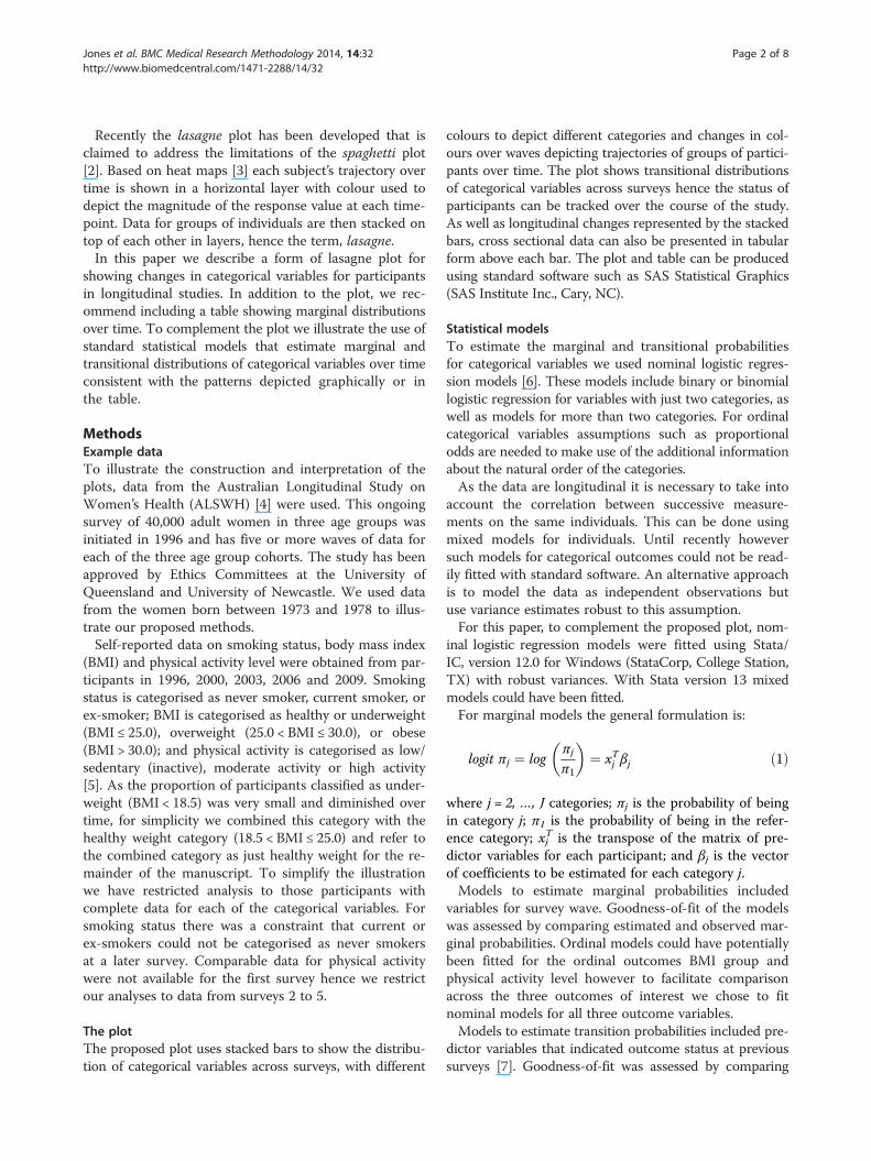
Jones et al. BMC Medical Research Methodology 2014, 14:32 Page 2 of 8http://www.biomedcentral.com/1471-2288/14/32

Recently the lasagne plot has been developed that isclaimed to address the limitations of the spaghetti plot[2]. Based on heat maps [3] each subject’s trajectory overtime is shown in a horizontal layer with colour used todepict the magnitude of the response value at each time-point. Data for groups of individuals are then stacked ontop of each other in layers, hence the term, lasagne.In this paper we describe a form of lasagne plot for

showing changes in categorical variables for participantsin longitudinal studies. In addition to the plot, we rec-ommend including a table showing marginal distributionsover time. To complement the plot we illustrate the use ofstandard statistical models that estimate marginal andtransitional distributions of categorical variables over timeconsistent with the patterns depicted graphically or inthe table.

MethodsExample dataTo illustrate the construction and interpretation of theplots, data from the Australian Longitudinal Study onWomen’s Health (ALSWH) [4] were used. This ongoingsurvey of 40,000 adult women in three age groups wasinitiated in 1996 and has five or more waves of data foreach of the three age group cohorts. The study has beenapproved by Ethics Committees at the University ofQueensland and University of Newcastle. We used datafrom the women born between 1973 and 1978 to illus-trate our proposed methods.Self-reported data on smoking status, body mass index

(BMI) and physical activity level were obtained from par-ticipants in 1996, 2000, 2003, 2006 and 2009. Smokingstatus is categorised as never smoker, current smoker, orex-smoker; BMI is categorised as healthy or underweight(BMI ≤ 25.0), overweight (25.0 < BMI ≤ 30.0), or obese(BMI > 30.0); and physical activity is categorised as low/sedentary (inactive), moderate activity or high activity[5]. As the proportion of participants classified as under-weight (BMI < 18.5) was very small and diminished overtime, for simplicity we combined this category with thehealthy weight category (18.5 < BMI ≤ 25.0) and refer tothe combined category as just healthy weight for the re-mainder of the manuscript. To simplify the illustrationwe have restricted analysis to those participants withcomplete data for each of the categorical variables. Forsmoking status there was a constraint that current orex-smokers could not be categorised as never smokersat a later survey. Comparable data for physical activitywere not available for the first survey hence we restrictour analyses to data from surveys 2 to 5.

The plotThe proposed plot uses stacked bars to show the distribu-tion of categorical variables across surveys, with different

colours to depict different categories and changes in col-ours over waves depicting trajectories of groups of partici-pants over time. The plot shows transitional distributionsof categorical variables across surveys hence the status ofparticipants can be tracked over the course of the study.As well as longitudinal changes represented by the stackedbars, cross sectional data can also be presented in tabularform above each bar. The plot and table can be producedusing standard software such as SAS Statistical Graphics(SAS Institute Inc., Cary, NC).

Statistical modelsTo estimate the marginal and transitional probabilitiesfor categorical variables we used nominal logistic regres-sion models [6]. These models include binary or binomiallogistic regression for variables with just two categories, aswell as models for more than two categories. For ordinalcategorical variables assumptions such as proportionalodds are needed to make use of the additional informationabout the natural order of the categories.As the data are longitudinal it is necessary to take into

account the correlation between successive measure-ments on the same individuals. This can be done usingmixed models for individuals. Until recently howeversuch models for categorical outcomes could not be read-ily fitted with standard software. An alternative approachis to model the data as independent observations butuse variance estimates robust to this assumption.For this paper, to complement the proposed plot, nom-

inal logistic regression models were fitted using Stata/IC, version 12.0 for Windows (StataCorp, College Station,TX) with robust variances. With Stata version 13 mixedmodels could have been fitted.For marginal models the general formulation is:

logit πj ¼ logπj

π1

� �¼ xTj βj ð1Þ

where j = 2, …, J categories; πj is the probability of beingin category j; π1 is the probability of being in the refer-ence category; xj

T is the transpose of the matrix of pre-dictor variables for each participant; and βj is the vectorof coefficients to be estimated for each category j.Models to estimate marginal probabilities included

variables for survey wave. Goodness-of-fit of the modelswas assessed by comparing estimated and observed mar-ginal probabilities. Ordinal models could have potentiallybeen fitted for the ordinal outcomes BMI group andphysical activity level however to facilitate comparisonacross the three outcomes of interest we chose to fitnominal models for all three outcome variables.Models to estimate transition probabilities included pre-

dictor variables that indicated outcome status at previoussurveys [7]. Goodness-of-fit was assessed by comparing

Jones et al. BMC Medical Research Methodology 2014, 14:32 Page 3 of 8http://www.biomedcentral.com/1471-2288/14/32

estimated and observed transition probabilities as well ascalculating McFadden’s pseudo R2 which is an estimate ofthe magnitude of improvement of the fitted model com-pared to the uninformative or null model [8]. We also cal-culated the proportion of correct predictions provided bythe final model and contrasted the result with the propor-tion of correct predictions from an uninformative modelwhere no explanatory variables were fitted. The deltamethod was used to estimate standard errors for transi-tion probabilities so that 95% confidence intervals couldbe calculated.To guide our decision on how many previous surveys

to include as explanatory information in the models, weestimated variance inflation factors (VIF) and percentageincreases in log likelihood. We preferred percentage in-creases in log likelihood to the more common approachof using absolute increases to assess model fit becausethey are more informative in terms of predictability forindividuals. As an additional visual tool to illustrate dis-tributions of outcome variables over time, probabilitytree diagrams depicting proportions of participants ineach response category at each wave were used to assistwith constructing the transition models.

ResultsThe plotThe proposed plots are shown in Figures 1, 2 and 3 forphysical activity level, BMI group and smoking status

Figure 1 Plot and marginal distribution table of physical activity leveWomen’s Health.

respectively. Informally comparing the three outcomevariables, it appears participants were more likely tochange physical activity level between surveys thanBMI group or smoking status. However BMI categorycannot change as quickly as levels of physical activityor smoking status. Also it was not possible to becomea never smoker after being a smoker. The plots sug-gest predictability of physical activity level for individ-uals over time would be low whereas predictabilitywould be better for BMI group and perhaps even bet-ter for smoking status. See Additional file 1 for SAScode we used for the smoking status plot. To investi-gate predictability of individuals over time further weused more formal procedures.

Marginal modelsMarginal nominal logistic models for all three outcomevariables showed approximately linear changes in logrelative risk ratios (RRR) over surveys hence survey wasfitted as a numerical variable:

logit πj ¼ β1j þ Survey� β2j ð2Þ

where Survey = 2, …, 5.Predicted probabilities from the fitted models had con-

sistently high agreement with the observed probabilitieswith absolute differences within 1-2% in all cases (datanot shown). Compared to being inactive the relative risk

l over survey wave for the Australian Longitudinal Survey of

Figure 2 Plot and marginal distribution table of body mass index group over survey wave for the Australian Longitudinal Survey ofWomen’s Health.

Jones et al. BMC Medical Research Methodology 2014, 14:32 Page 4 of 8http://www.biomedcentral.com/1471-2288/14/32

of being in the moderate physical activity category de-creased at each survey by 7% (RRR = 0.93; 95% CI:0.90, 0.95) and the relative risk of being in the highphysical activity category decreased at each survey by14% (RRR = 0.86; 95% CI: 0.85, 0.88). With healthy

Figure 3 Plot and marginal distribution table of smoking status over sur

weight as the reference group, the relative risk of be-ing in a higher BMI category increased at each survey(RRR= 1.17; 95% CI: 1.15, 1.20 for overweight and RRR=1.32; 95% CI: 1.29, 1.34 for obese). For smoking status, wherenever smokers was the reference category, the relative risk

vey wave for the Australian Longitudinal Survey of Women’s Health.

Table 2 Relative risk ratios based on transitional modelfor BMI group (reference = overweight)

Outcome Predictor variable Relative risk ratio(95% confidence interval)

Healthy weight Previously healthy weight 14.2 (12.2, 16.5)

Jones et al. BMC Medical Research Methodology 2014, 14:32 Page 5 of 8http://www.biomedcentral.com/1471-2288/14/32

of being an ex-smoker increased (RRR 1.17; 95% CI: 1.15,1.19) whereas the relative risk of being a current smokerdecreased at each survey (RRR 0.81; 95% CI: 0.79, 0.82).

Transitional modelsResults for physical activity showed VIFs that were lessthan 1.5 for inclusion of explanatory variables at anynumber of previous surveys. Percentage increases in loglikelihood were modest generally and less than 1% fortwo and three previous surveys (Table 1). Based on theseresults we included just the previous survey in the tran-sition model for physical activity. Our proposed transi-tion model equation for physical activity was:

logit πj ¼ β1j þ I Moderateð Þ−1 � β2j

þ I Highð Þ−1 � β3j ð3Þ

where I(Moderate)−1 indicates moderate activity level atthe previous survey and Ι(High)−1 indicates high activitylevel at the previous survey.Model estimates showed that previous moderate activ-

ity was associated with an 80% increased relative risk ofcurrent moderate activity (RRR 1.84; 95% CI: 1.65, 2.04)and more than a doubling in relative risk of current highactivity (RRR 2.15; 95% CI: 1.93, 2.40). In addition previ-ous high activity is associated with a more than doublingin relative risk of current moderate activity (RRR 2.33;95% CI: 2.09, 2.59) and a more than five-fold increase inrelative risk of current high activity (RRR 5.40; 95% CI:4.87, 5.99). Pseudo R2 for the fitted model was 4.5% andthe proportion of correct predictions was 56% (com-pared to 53% correct predictions for an uninformativemodel) indicating a poor predictability of physical activ-ity level for individuals based on previous survey results.However predicted probabilities from the fitted modelagreed with the observed probabilities to within 1% forall comparisons indicating a good overall model fit. Esti-mated transition probabilities showed that previous mod-erate activity was associated with a 47% (95% CI: 45%,48%) probability of current low or sedentary activity, a 27%(95% CI: 26%, 29%) probability of current moderate activityand a 26% (95% CI: 24%, 28%) probability of current high

Table 1 Percentage changes in log likelihood

Variableat surveywave 5

Nullmodel

Previoussurvey

Twosurveysprevious

Threesurveysprevious

Physical activity level −8062.1 −7703.1 −7648.9 −7601.2

4.5% +0.6% +0.6%

BMI group −8644.0 −4811.2 −4562.8 −4506.7

44.3% +2.9% +0.6%

Smoking status −10906.3 −2588.4 −2449.6 −2424.8

76.3% +1.2% +0.2%

activity. Previous high activity was associated with a 32%(95% CI: 30%, 33%) probability of current low or sedentaryactivity, a 24% (95% CI: 22%, 25%) probability of currentmoderate activity and a 44% (95% CI: 43%, 46%) probabilityof current high activity. Previous low or sedentary activitywas associated with a 63% (95% CI: 62%, 64%) probabilityof current low or sedentary activity, a 20% (95% CI: 19%,21%) probability of current moderate activity and a 16%(95% CI: 15%, 17%) probability of current high activity.For BMI group, based on all VIFs being less than 3 and

percentage increases in log likelihood as shown in Table 1,the BMI categories for the two previous surveys were in-cluded in the transition model. The reference category waschosen to be the overweight group as this ensured the esti-mated relative risk ratios and standard errors were stable.The transition model equation for BMI group was:

logit πj ¼ β1j þ I Healthyð Þ−1 � β2j þ I Obeseð Þ−1 � β3j

þ I Healthyð Þ−2 � β4j þ I Obeseð Þ−2 � β5j

ð4Þwhere Ι (Healthy)−1 indicates healthy weight at the previ-ous survey, Ι (Obese)−1 indicates obesity at the previoussurvey, Ι (Healthy)−2 indicates healthy weight two surveyspreviously, and Ι (Obese)−2 indicates obesity two surveyspreviously.Table 2 shows estimated relative risk ratios and 95%

confidence intervals obtained from the transition model.Pseudo R2 for the model was 0.47 with 81% correct pre-dictions (compared to 59% correct predictions for anuninformative model) indicating moderate predictabilityof current BMI group for individuals based on BMI groupat the two previous surveys. Predicted and observed tran-sitional probabilities showed only moderate agreement, al-though some of these categories included low numbers ofparticipants (Additional file 2: Figure S1).

Healthy weight Previously obese 0.83 (0.47, 1.44)

Healthy weight Healthy weight twosurveys previously

5.11 (4.22, 6.18)

Healthy weight Obese two surveyspreviously

0.68 (0.35, 1.35)

Obese Previously healthy weight 0.20 (0.13, 0.29)

Obese Previously obese 11.6 (9.20, 14.5)

Obese Healthy weight twosurveys previously

0.59 (0.47, 0.75)

Obese Obese two surveyspreviously

2.92 (2.25, 3.80)

Jones et al. BMC Medical Research Methodology 2014, 14:32 Page 6 of 8http://www.biomedcentral.com/1471-2288/14/32

For smoking status, VIFs of between 6 and 24 indi-cated strong multicollinearity when more than one pre-vious survey was included as explanatory information ina transition model. However we were able to include anexplanatory variable indicating whether or not a partici-pant was an ex-smoker two surveys previously as thisdid not result in multicollinearity and added useful pre-dictive information to the model. Figure 4 shows a prob-ability tree diagram for current smokers illustrating theadditional predictive value of including being an ex-smoker two surveys previously as a predictor variable. Incontrast, being a current smoker two surveys previouslyadded little additional predictive value. Transitions frombeing an ex- or current smoker to never having smokedare not possible hence current smoker was chosen asthe reference category and predictor coefficients indi-cating previous smoking status of never smokers wereconstrained to be (structurally) zero. Some participantsreported never smoking after being classified as an ex-smoker or current smoker at earlier surveys. These partici-pants were reclassified as ex-smokers. The transition model(shown below) included indicator variables for whetherthe participant was a current smoker in the previous sur-vey, an ex-smoker at the previous survey, or an ex-smokerat the previous two surveys.

logit πj ¼ β1j þ I Exð Þ−1 � β2j þ I Currentð Þ−1 � β3j

þ I Exð Þ−1;−2 � β4j ð5Þ

Current smoker

N=1367

Ex-smoker

N=432 (32%)

Current smoker

N=935 (68%)

Figure 4 Probability tree for current smoker over survey waves 2–5.

where -1 indicates status at the previous survey, -1,-2 indi-cates ex-smoker for both previous surveys.Estimates obtained from the model showed that being

an ex-smoker at the previous survey (but not being anex-smoker two surveys previously) was associated with adoubling in relative risk of being an ex-smoker currently(RRR 2.01; 95% CI: 1.12, 3.63) whereas being an ex-smoker for both previous surveys was associated with a12-fold increased relative risk of being an ex-smokercurrently (RRR 12.8; 95% CI: 6.95, 23.5). Being a currentsmoker at the previous survey was associated with a72% lower relative risk of being an ex-smoker currently(RRR 0.28; 95% CI: 0.16, 0.50). The final model hadpseudo R2 = 0.77 with 91% correct predictions (comparedto 52% correct predictions for an uninformative model)hence smoking status for the previous surveys was highlypredictive of current status for individuals. Predicted andobserved transitional probabilities agreed to within 1% inall cases hence goodness-of-fit statistics indicated themodel fitted the observed data well. Predicted probabilitiesshowed previous never smokers had 99% (95% CI: 98.8%,99.3%) chance of being a never smoker at the current sur-vey, 0.6% (95% CI: 0.4%, 0.8%) chance of being an ex-smoker and 0.3% (95% CI: 0.1%, 0.5%) chance of being acurrent smoker. Previous current smokers had 34% (95%CI: 32%, 37%) chance of being an ex-smoker in thecurrent survey and 66% (95% CI: 63%, 68%) of being acurrent smoker. An ex-smoker for the two previous sur-veys had 4% (95% CI: 3%, 5%) chance of being a current

Ex-smoker

N=341 (79%)

Ex-smoker

N=313 (92%)

Current smoker

N=28 (8%)

Current smoker

N=91 (21%)

Ex-smoker

N=47 (52%)

Current smoker

N=44 (48%)

Ex-smoker

N=260 (28%)

Ex-smoker

N=192 (74%)

Current smoker

N=68 (26%)

Current smoker

N=675 (72%)

Ex-smoker

N=205 (30%)

Current smoker

N=470 (70%)

Jones et al. BMC Medical Research Methodology 2014, 14:32 Page 7 of 8http://www.biomedcentral.com/1471-2288/14/32

smoker at the current survey and 96% (95% CI: 95%, 97%)chance of being an ex-smoker. However for ex-smokers atthe previous survey, who were not ex-smokers two sur-veys previously, the transition probabilities were 21% (95%CI: 18%, 24%) for current smoking and 79% (95% CI: 76%,82%) for ex-smoking.

DiscussionThe plot we have illustrated visually depicts changes incategorical variables for individuals over time. Howeverthe marginal distribution at follow up time-points is notas clearly shown, therefore we recommend inclusion of atable above the stacked bars showing the marginal distri-bution at each time-point. Simple nominal logistic re-gression models can be used to formalise the visualinformation provided by the plot and estimate marginaland transitional probabilities as well as relative effects.Probability tree diagrams are useful in helping developthe models.Transitional probabilities, in particular, provide useful

and easily interpretable summary information. For ex-ample, based on ALSWH data, conditional on beingoverweight for two previous surveys, Australian womenin their twenties had 23% (95% CI: 21%, 26%) probabilityof being obese at the next survey but only 7% (95% CI:6%, 9%) probability of being of healthy weight (or under-weight). We suggest McFadden’s pseudo R2 as a sum-mary measure for assessing predictability of categoricaloutcomes and, to guide decisions on how many previousmeasures should be included in the transition models,we propose using variance inflation factors and percent-age increases in log likelihood.Spaghetti plots are very useful for showing changes in

a numerical variable for a limited number of individualsover time but are not applicable for categorical data orlarge numbers of individuals. Lasagne plots have beenproposed as an alternative to spaghetti plots for categor-ical data and/or many individuals. There are howeverseveral other methods for graphically representing cat-egorical data but they have a number of limitations. Forexample, in the mosaic plot the relative frequency ofeach level of a variable and its relationship to another vari-able is represented by a mosaic of tiles [9]; see Additionalfile 3: Figure S2. A variable degree of shading for each tileis then incorporated to represent the degree of deviationfrom a null hypothesis of independence. However addingmore variables increases complexity and showing the dis-tribution of a categorical variable over multiple waves of alongitudinal survey is not feasible.Another technique is known as parallel sets [10]; a simi-

lar concept to Sankey diagrams [11]. In these diagrams therelationship between variables is shown using parallelo-grams whose width is proportional to the frequenciesinvolved (Additional file 4: Figure S3). Parallel sets are

appropriate for categorical data collected on large num-bers of participants over multiple surveys but the plotlacks simplicity and software to produce the figures isnot readily available.The lasagne plot we illustrate offers some advantages

over these alternative methods in terms of ease of depic-tion and interpretation. But, irrespective of which graph-ical method is used, the information obtained is onlydescriptive hence the need for methods that allow formaltesting and estimation.To simplify our illustration we restricted analysis to in-

dividuals who provided complete responses over foursurveys. However this restriction could be relaxed to in-clude all participants. In this case missing data couldform an additional category and be included in the plot,tabulation and models. The addition of a missing datacategory could provide additional insights into the data.For example, it could show that certain categories in pre-vious surveys are associated with increased risk of missingdata in subsequent surveys. It may also be of interest totabulate the patterns of missing data across surveys. Weillustrate the inclusion of missing data as a category in thegraphical analysis of BMI categorised into healthy, over-weight/obese, or missing (Additional file 5: Figure S4).The plot suggests previous missingness predicts currentmissingness but missingness does not appear to be associ-ated with the other BMI categories of healthy weight andoverweight/obese.A limitation of the lasagne plot is that it is not

feasible to include a large number of categories. Inour example we used three categories. Including morecategories would make interpretation increasingly dif-ficult. We therefore recommend four categories atmost. If there are more than four categories then werecommend collapsing the data into fewer categories.For physical activity level, for example, we collapsedsedentary and low activity into “inactive”. Continuousvariables could also be summarised using these methodshowever they would require categorisation with conse-quential loss of detail. A further limitation is that thenumber of categories shown at later time-points can behigh making interpretation difficult. If this is the casewe suggest making separate plots of transitions fromeach individual category at the initial survey to sup-plement the overall plot. We illustrate this idea for smok-ing status in Additional file 6: Figures S5 and Additionalfile 7: S6. Finally we have illustrated the plot and modelswith data from a longitudinal survey where the partici-pants have been assessed at regular periods over time. Ifdata had been collected at irregular time-points, ourmethodology may not be appropriate. Despite these limi-tations, we believe the plot and models are appropriatein general for categorical variables collected in longi-tudinal studies.

Jones et al. BMC Medical Research Methodology 2014, 14:32 Page 8 of 8http://www.biomedcentral.com/1471-2288/14/32

ConclusionsThe lasagne plot we illustrate provides a simple way toshow transitions in the status of individuals observedlongitudinally. The regression models we suggest com-plement the plots and allow formal testing and reportingof marginal and transitional distributions. These analyt-ical tools can be implemented in standard statistical soft-ware such as SAS and Stata and can provide valuableinsights into categorical variables measured on individualsat regular intervals over time.

Additional files

Additional file 1: SAS code for generating smoking status plot.

Additional file 2: Figure S1. Probability tree diagram for BMI groupwith observed and estimated transitional probabilities and 95%confidence intervals in brackets.

Additional file 3: Figure S2. Mosaic plot of smoking status at surveywave 1 compared to wave 2.

Additional file 4: Figure S3. Parallel sets diagram of smoking statustransitions from survey waves 1 to 5.

Additional file 5: Figure S4. Plot and marginal distribution table ofbody mass index group with a missing category over survey wave for theAustralian Longitudinal Survey of Women’s Health.

Additional file 6: Figure S5. Plot and marginal distribution table ofsmoking status over survey wave for ex-smokers at survey wave 2.

Additional file 7: Figure S6. Plot and marginal distribution table ofsmoking status over survey wave for current smokers at survey wave 2.

AbbreviationsALSWH: Australian Longitudinal Study of Women’s Health; BMI: Body massindex; VIF: Variance inflation factor; RRR: Relative risk ratio.

Competing interestThe authors declare that they have no competing interest.

Authors’ contributionRH developed the plot methodology; MJ developed the modelling strategyand wrote the manuscript; GM and AD oversaw the project, providedsupervision as well as critical input into the design and implementation;all authors reviewed and/or revised the manuscript and have approved it forsubmission.

AcknowledgementsFunding: The Australian Longitudinal Study on Women’s Health is funded bythe Australian Department of Health. MJ and GDM are funded by theAustralian National Health and Medical Research Council (APP1000986). RH isfunded by the Australian Department of Health and AD is funded by theUniversity of Queensland. The funding bodies had no role in the collection,analysis, and interpretation of data; the writing of the manuscript, or thedecision to submit the manuscript for publication. There was no additionalperson who contributed materials essential for the study or who contributedto the preparation of this article.

Received: 18 November 2013 Accepted: 21 February 2014Published: 27 February 2014

References1. Hedeker D, Gibbons R: Longitudinal data analysis. Hoboken, New Jersey:

John Wiley and Sons; 2006.2. Swihart B, Caffo B, James B, Strand M, Schwartz B, Punjabi N: Lasagna plots:

a saucy alternative to spaghetti plots. Epidemiology 2010, 21:621–625.3. Wilkinson L, Friendly M: The history of the cluster heat map. Am Stat 2009,

63:179–184.

4. Dobson AJ, Barnett A: An Introduction to Generalized Linear Models. 3rdedition. Boca Raton, Florida: Chapman & Hall/CRC; 2008.

5. Lee C, Dobson AJ, Brown WJ, Bryson L, Byles J, Warner-Smith P, Young AF:Cohort profile: the Australian Longitudinal Study on Women's Health.Int J Epidemiol 2005, 34:987–991.

6. Brown WJ, Trost SG: Life transitions and changing physical activitypatterns in young women. Am J Prev Med 2003, 25:140–143.

7. Ware J, Lipsitz S, Speizer F: Issues in the analysis of repeated categoricaloutcomes. Stat Med 1988, 7:95–107.

8. Long J: Regression Models for Categorical and Limited Dependent Variables.Thousand Oaks: Sage Publications; 1997.

9. Friendly M: Mosaic displays for multi-way contingency tables. J Am StatAssoc 1994, 89:190–200.

10. Kosara R: Parallel sets: interactive exploration and visual analysis ofcategorical data. Trans on Visualization and Comput Graph 2006, 12:1–12.

11. Schmidt M: Der Einsatz von sankey-diagrammen im stoffstrommanagement.Beitraege der Hochschule Pforzheim 2006. Nr. 124.

doi:10.1186/1471-2288-14-32Cite this article as: Jones et al.: Visualising and modelling changes incategorical variables in longitudinal studies. BMC Medical ResearchMethodology 2014 14:32.

Submit your next manuscript to BioMed Centraland take full advantage of:

• Convenient online submission

• Thorough peer review

• No space constraints or color figure charges

• Immediate publication on acceptance

• Inclusion in PubMed, CAS, Scopus and Google Scholar

• Research which is freely available for redistribution

Submit your manuscript at www.biomedcentral.com/submit