Areal Interpolation of Population Counts Using Pre-classified Land Cover Data

Areal Interpolation of Population CountsUsing Pre-classified Land Cover Data

Michael Reibel Æ Aditya Agrawal

Published online: 19 September 2007

� Springer Science+Business Media B.V. 2007

Abstract The need to combine spatial data representing sociodemographic

information across incompatible spatial units is a common problem for demogra-

phers. A particular concern is computing small area trends when aggregation zone

boundaries change during the trend interval. To that end, this study provides an

example of dasymetric areal interpolation using the pre-classified land cover data

available through the US Geological Survey’s National Land Cover Dataset

(NLCD) program. Areal interpolation of population estimates is preferable to tra-

ditional reaggregation techniques, and the use of land cover data as a weighting

factor in interpolated estimation has been shown in earlier studies to be highly

accurate. In this study, the NLCD data set performs well and, because it requires no

classification, it compares favorably with other land cover data sets for areal

interpolation when considered on the basis of accuracy, precision and ease of use.

Keywords Areal interpolation � Population estimates � Census geography �GIS

Introduction

This study proposes an approach to accurate areal interpolation using pre-classified

land use data as a solution to common problems requiring the combination of

incompatible spatial data, e.g., temporal analyses of sociodemographic trends from

census tracts. We begin by discussing the problem and the traditional solution of

M. Reibel (&)

Department of Geography and Anthropology, California State Polytechnic University – Pomona,

3801 W. Temple Place, Pomona, CA 91768, USA

e-mail: [email protected]

A. Agrawal

Redlands Institute, University of Redlands, Redlands, CA, USA

123

Popul Res Policy Rev (2007) 26:619–633

DOI 10.1007/s11113-007-9050-9

reaggregation to create a synthetic system of compatible zones. A discussion of

areal interpolation using Geographic Information Systems (GIS) follows, including

a description of the steps involved that can be followed by demographers with

access to a GIS. We propose the US Geological Survey’s National Land Cover

Dataset (NLCD) as a highly suitable spatial data layer for performing areal

interpolation of spatially aggregated incompatible data.

We will then present a case study test of the accuracy of tract level population

estimates computed using the NLCD and dasymetric areal interpolation. Interpo-

lated estimates are benchmarked against a reference set of tract population counts

generated from block counts, and the computed errors are mapped, analyzed, and

compared to the corresponding error distribution of a set of estimates interpolated

using a simpler technique with more restrictive assumptions. In light of these

findings, dasymetric areal interpolation using the NLCD layer is evaluated relative

to alternative techniques with respect to count accuracy, geographic precision, and

ease of computation.

Theoretical Background

An important methodological problem in spatial demography is the frequent need to

combine incompatible spatial data (Gotway and Young 2002). Incompatibility, in

such situations, means data that are aggregated (or coded, in the case of microdata)

to two or more superimposed zone systems must be combined in a single record for

analysis (cf. Flowerdew and Green 1989), and that some zones in either or both zone

systems extend across the territory of two or more zones in another zone system. If,

within the study area, all zones in each of the relevant zone systems can be either

aggregated completely into whole zones or treated in their entirety as aggregations

of whole zones of each other zone system, the systems are nested with respect to

each other. Thus, in nested zone systems, whole zones in one zone system can be

reaggregated to areas corresponding perfectly to one or more zones in the other

systems, and the attribute counts pertaining to the aggregated zones can be summed

to create compatible counts.

A common corresponding problem of incompatible spatial data in demography is

the need to combine tract level population and subpopulation count data for the

same region pertaining to two successive census enumerations, in order to compute

an exhaustive and mutually exclusive set of tract level trends for the time interval.

Other studies, notably in the contextual effects modeling of microdata and in the

metropolitan analysis of microdata, have encountered similar difficulty in the

geoprocessing of data aggregated to incompatible area units. For a detailed

discussion of the problem, and the evolution of solutions including areal

interpolation, see the review article by Reibel (2007) in this issue.

In the past, investigators have typically sought to solve the problem of combining

spatially mismatched data by reaggregating area units from two superimposed zone

systems to the zone coverage containing the smallest possible compatible

reaggregation zones. Compatible reaggregation zones are a synthetic zone system

consisting only of one or more whole area units in both original zone systems to

620 M. Reibel, A. Agrawal

123

which data are aggregated. In other words, for maximum efficiency zones are

reaggregated in both directions, from zone system A to zone system B where B

zones are composed of multiple A zones and vice versa. It is not always necessary

for zones to be nested in order to create compatible reaggregation zones.

It is sometimes possible to reaggregate areas where zones from one system

extend across two or more of the second system’s zones using only whole zones

from both zone systems. But this normally requires that a larger number of zones in

both systems be combined, often resulting in synthetic reaggregation zones that are

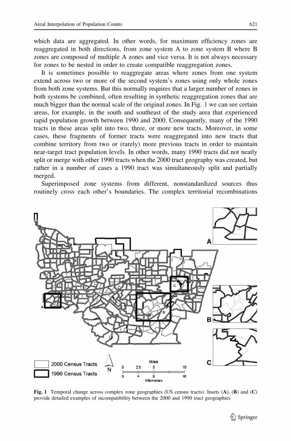
much bigger than the normal scale of the original zones. In Fig. 1 we can see certain

areas, for example, in the south and southeast of the study area that experienced

rapid population growth between 1990 and 2000. Consequently, many of the 1990

tracts in these areas split into two, three, or more new tracts. Moreover, in some

cases, these fragments of former tracts were reaggregated into new tracts that

combine territory from two or (rarely) more previous tracts in order to maintain

near-target tract population levels. In other words, many 1990 tracts did not neatly

split or merge with other 1990 tracts when the 2000 tract geography was created, but

rather in a number of cases a 1990 tract was simultaneously split and partially

merged.

Superimposed zone systems from different, nonstandardized sources thus

routinely cross each other’s boundaries. The complex territorial recombinations

Fig. 1 Temporal change across complex zone geographies (US census tracts). Insets (A), (B) and (C)provide detailed examples of incompatibility between the 2000 and 1990 tract geographies

Areal Interpolation of Population Counts 621

123

typical of geographic area changes over time for census tracts and other data series

aggregation zones, and other such mismatches, frequently lead to situations in

which systems of hundreds of zones would need to be reduced to fewer than ten

reaggregation zones in order to match geographies. Such an outcome renders

appropriate-scale analysis of local variation within a region impossible. To cope

with these situations, investigators must choose between extreme exaggeration in

the scale of some zones included in their analyses, or deleting the observations

associated with the troublesome zones.

Areal interpolation is a more elegant and, with the use of geographic information

systems (GIS), often easier solution to matching incompatible data aggregation

zones than the reaggregation approaches described above (Gotway and Young 2002;

Eicher and Brewer 2001; Goodchild et al. 1993; Bracken and Martin 1989).

Moreover, because reaggregation inevitably involves situations in which complex

boundary changes leave analysts with no solution that would preserve both the

processing protocol and the appropriate scale of area units, areal interpolation can

be assumed to be more geographically precise and more reliably exhaustive of the

study area territory. Areal interpolation refers broadly to techniques that assign data

from one or more sets of geographic areas to which data are aggregated (the source

zones) to another incompatible and superimposed set (the target zones) using spatial

algorithms. In current practice, most of these algorithms exploit the map overlay

capabilities of GIS (Longley et al. 2005).

The simplest type of areal interpolation is area weighted interpolation, which

requires no information besides the geography of both sets of zone units and the

counts to be interpolated from the source to the target zones (Goodchild and Lam

1980). In area weighted interpolation the two incompatible zone systems describing

a given region are superimposed and intersected, creating a set of intersection zones,

each of which describes a unique pair of one source and one target zone (Flowerdew

and Green 1992). Each intersection zone is assigned a fraction of its respective

source zone’s count corresponding to the proportion of the source zone’s area

occupied by the intersection zone. The intersection zone counts can then be summed

across their respective target zones to complete the integration of data to the

incompatible zone system.

It is immediately apparent that area weighted interpolation relies on the

assumption that there are no internal variations in count density within any source

zone, an assumption that is not generally warranted. All other area interpolation

techniques seek to improve the accuracy of estimates by bringing to bear

meaningful information regarding local density variations of counts within the

source zones. Pycnophylactic smoothing techniques use the density surface of the

set of source tract counts themselves, and create fine-grained, smooth estimated

density gradients inside the source tracts by interpolating each tract’s count

internally based on the count densities of adjacent tracts (Tobler 1979). The

resulting estimated population surface can be used as locally detailed geographic

information as is, or it can be reaggregated to another zone system that is

incompatible with the first. These smoothing techniques, however, require a

relatively high level of geostatistical and geoprocessing skill, and can introduce

error when (as is the case with census tracts) count density gradients are not in fact


123

typically smooth up to and beyond tract boundaries. Indeed, census tracts frequently

have abrupt population density changes that coincide with the distinctive features in

the built environment (such as major highways and strips of abandoned brown

fields) that are typically chosen as tract boundaries.

The other general approach to areal interpolation that seeks to apply

information about internal source zone density gradients involves the use of

(typically fine-grained) ancillary data layer that is used as a proxy for count

densities. This additional layer is superimposed on the source zones from which

counts are to be interpolated, and counts are reassigned to the geography

corresponding to the ancillary data values according to derived algorithms. The

estimated counts are then reaggregated from this proxy geography to the set of

target zones.

The algorithms typically used to assign source zone counts to areas in the

ancillary weighting geography fall into two major types. The first we will call

homogenous source zone weighting, and the second is regression weighting. In

homogenous source zone weighting, the analyst identifies source zones each of

which consists entirely of territory corresponding to a single ancillary weighting

data value (Mennis 2003; Eicher and Brewer 2001). In order to be practicable, the

technique requires at least one source zone associated with each potential

categorical value of the ancillary weighting scheme. The analyst then pools the

populations and areas of source zones corresponding to each ancillary weight value

to derive a population density estimate for that value. These estimates can then be

applied per unit area to the entire system, including source zones with fragmented

ancillary weighting geographies.

Regression weighted areal interpolation fits the source zone counts by regressing

them on the areas of each source zone corresponding to the set of ancillary data

values (Flowerdew and Green 1989, 1992). The resulting coefficients for each

ancillary data value are the densities, i.e., the estimated populations per unit area of

that ancillary data value.

A considerable variety of ancillary data layers has been brought to bear for

purposes of areal interpolation, with corresponding variation in the difficulty of

spatial data processing and the quality of results. Most studies have used remotely

sensed urban land cover surface data as a weighting factor, but some have used

objects such as the street grid (Reibel and Bufalino 2005), or control zones

corresponding to functional areas (Reibel and Agrawal 2005; Goodchild et al.

1993). Areal interpolation using remotely sensed urban land cover data (Fisher and

Langford 1996; Langford and Unwin 1994) as well as Reibel and Bufalino’s (2005)

street weighting technique have proven to be relatively accurate. Moreover, the

larger number of studies using land cover data, and the robust tests documenting its

accuracy, including resampling simulations in Cockings et al. (1997), makes land

cover weighting the normative approach to areal interpolation. The major difficulty

of urban land cover weighted areal interpolation until now has been the need to

transform raw images into an information surface, a difficult procedure called

digital image processing or classification (Schowengerdt 1997; Jensen 1996;

Lillesand and Kiefer 1987).


123

Data and Methods

This study provides an applied example and test of urban land cover weighted areal

interpolation using a detailed pre-classified land cover data layer. These data and

methods are a good fit for demographers who use GIS but are not GIS specialists

because they offer the power and accuracy of land cover weighted interpolation

without the need to classify remotely sensed images. Our approach uses land cover

data derived through the National Oceanic and Atmospheric Administration’s

(NOAA) Coastal Change Analysis (C-CAP)1 Program. Because these data are

integrated into the US Geological Survey’s National Land Cover Dataset (NLCD),

we hereafter refer to the data as the NLCD. The NLCD data are free, seamless, and

downloadable from http://seamless.usgs.gov/website/seamless/viewer.php. These

high quality data, derived from Landsat satellite images, provide pre-classified

information on land cover category types, including urban land cover, at 30 m

resolution for the entire United States. We will provide a set of steps to guide

investigators as they perform interpolations using these data, as well as a discussion

and examination of the estimation errors in the interpolated population counts in our

example.

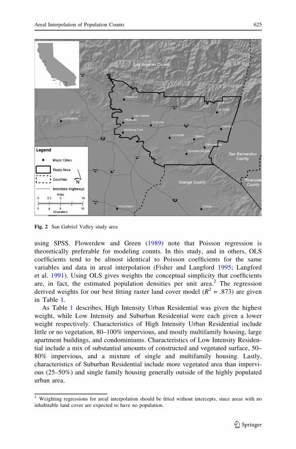
In this example, we will perform land cover weighted areal interpolation using

the NLCD to interpolate 2000 census tract population counts in a study area for

eastern Los Angeles County to the 1990 census tract geography. The study area

consists of the San Gabriel Valley region and adjacent areas to the east extending to

the border of Los Angeles County (Fig. 2). The study area contains cities of over

100,000 persons, heavy industrial areas, dams and spillways, college campuses, old

citrus packing towns, low density suburbs and a border of hills and mountains.

Therefore, it is generally representative of the various landscapes within Los

Angeles County with the exception of coastal areas and the metropolitan central

business district.

The interpolation consists of a series of steps, mostly performed in a GIS

environment using ArcGIS 9.0 (Environmental Systems Research Institute,

Redlands CA). The weighting regression is performed in the statistical package

SPSS (SPSS Inc., Chicago IL). Most popular GIS packages lack integrated

regression and statistical analysis functionalities, but it is a simple matter to

transfer tabular data back and forth between the two packages by exporting the

tables to Dbase (.dbf) file format, which is accessible by both packages. The first

task is to fit a set of raster (grid cell) weights corresponding to inhabited land

cover types (uninhabited land cover types receive a weight of zero). To do this,

we computed the proportion of each source (2000) tract’s land area consisting of

30 · 30 m grid cells of each land cover type that might reasonably be expected

to be inhabited. Completely nonresidential land cover types are omitted from the

interpolation entirely; thus, none of the population of the set of source zones is

assigned to these areas. The tracts’ populations were then regressed on the areas

of inhabited land cover types using ordinary least squares (OLS) regression

1 Information about the NOAA’s C-CAP program and its integration into the USGS NLCD effort can be

found at http://www.csc.noaa.gov/crs/lca/ccap.html


123

http://seamless.usgs.gov/website/seamless/viewer.php

http://www.csc.noaa.gov/crs/lca/ccap.html

using SPSS. Flowerdew and Green (1989) note that Poisson regression is

theoretically preferable for modeling counts. In this study, and in others, OLS

coefficients tend to be almost identical to Poisson coefficients for the same

variables and data in areal interpolation (Fisher and Langford 1995; Langford

et al. 1991). Using OLS gives weights the conceptual simplicity that coefficients

are, in fact, the estimated population densities per unit area.2 The regression

derived weights for our best fitting raster land cover model (R2 = .873) are given

in Table 1.

As Table 1 describes, High Intensity Urban Residential was given the highest

weight, while Low Intensity and Suburban Residential were each given a lower

weight respectively. Characteristics of High Intensity Urban Residential include

little or no vegetation, 80–100% impervious, and mostly multifamily housing, large

apartment buildings, and condominiums. Characteristics of Low Intensity Residen-

tial include a mix of substantial amounts of constructed and vegetated surface, 50–

80% impervious, and a mixture of single and multifamily housing. Lastly,

characteristics of Suburban Residential include more vegetated area than impervi-

ous (25–50%) and single family housing generally outside of the highly populated

urban area.

Fig. 2 San Gabriel Valley study area

2 Weighting regressions for areal interpolation should be fitted without intercepts, since areas with no

inhabitable land cover are expected to have no population.


123

Once the weights have been computed, they are applied to the NLCD data layer’s

raster surface to generate a population surface map. However, because the model

accounts for only 87.3% of the variation in the source zone population, the weighted

estimates in the population surface must be scaled by the ratio of their respective

source zone’s observed population to its fitted population to account for the

proportion of source zone population not predicted in the model, thus preserving the

pycnophylactic property (Flowerdew and Green 1989, 1992). To do this, the grid

cells forming the raw estimated population surface were multiplied by the ratio of

their respective source tracts’ observed populations to the source tract’s fitted

population computed by summing the raw estimates across the source tract’s grid

cells:

GS ¼ GWTG

T̂G

� �;

where Gs is the scaled population estimate of grid cell G, GW is the raw weighted

population estimate of grid cell G, TG is the observed population of the source tract

of grid cell G, and T̂G is the fitted population of the source tract of grid cell Gderived by applying the weights to all grid cells and summing across all grid cells in

source tract T.

With respect to the regression derived weighting scheme, the values of the

predictor variables (i.e., categorical urban land cover types) are positively spatially

autocorrelated. Consequently, we can assume that the R-square statistic of the

weighting regression is somewhat inflated, and the weights themselves (i.e., the

coefficients associated with unit areas of each land use category) are inefficiently

estimated. It is important to recall, however, that the use of regression as one of a

series of data processing and estimation steps to derive weights in this example

serves a very different purpose from regression analysis for statistical inference. Our

subsequent step of scaling population estimates by the proportion of source zone

population unexplained by the regression, a practice pioneered by Flowerdew and

Green (1989, 1992), makes this explicit: such scaling, in effect, artificially raises the

explanatory power of the regression to its maximum limit (R2 = 1.0). The sequence

of procedures is not deterministic because of remaining between-tract variation in

the relationship between population density and the vector of urban land cover types

as pre-classified; that is the primary reason why (reduced) errors remain after

scaling. Taken together, however, the use of regression-derived weights and

pycnophylactic scaling are a practical solution that would be intolerable in

inferential statistics but which at least partially corrects for problems arising from

spatially autocorrelated predictor variables used to derive interpolation weights.

Table 1 Weights derived by

regression for inhabitable land

cover categories

Value Land cover type Weight

3 High intensity urban residential 0.808

4 Low intensity residential 0.374

5 Suburban residential 0.274

F statistic = 809.76 sig = .000


123

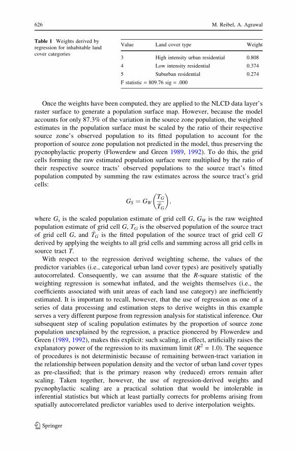
The result is the scaled population estimate surface map shown in Fig. 3.

Figure 3 shows the highly erratic and discontinuous nature of the study area’s

population distribution. Most of the less populated (thus lightly shaded) areas

consist of steep hills, with two major exceptions: the San Gabriel River flood plain

and quarrying area running southwest from the north central part of the map, and the

major industrial corridor along the Pomona Freeway that shows up as a light colored

upturned crescent in the southern central part of the map. Dense urban areas are

Pomona in the east, Pasadena in the northwest, and in the southwest, smaller dense

concentrations in the blue collar suburbs of Alhambra, El Monte and La Puente.

Next, the grid cells in the population surface map are reaggregated to the target

zone geography, 1990 census tracts in our case, and the grid cell estimates summed

across their respective target tracts to yield estimates of the source counts

interpolated to the target zones, i.e., the 2000 populations of the 1990 tracts.

The above steps complete the interpolation. Our test of the accuracy of the NLCD

land cover weighted interpolated population estimates requires three additional

steps: (1) the computation of a set of benchmark counts corresponding to the true

2000 populations of the 1990 tracts; (2) computation of the estimation errors via

subtraction from the benchmark counts; and (3) the exploration and analysis of the

error distribution. The benchmark counts for the 2000 populations of the 1990 tracts

Fig. 3 Scaled 2000 tract population counts derived from using the NLCD as a weighting layer wherepopulation estimates are now allocated to each 30 · 30 m grid cell


123

are computed by aggregating the 2000 census block counts to the 1990 census tract

geography, using the technique of block centroid aggregation described in Reibel

and Bufalino (2005). The errors in estimation computed by subtraction from these

benchmark observed counts are explored and mapped. Finally, the error distribution

and root mean square (RMS) errors for the NLCD weighted tract estimates and

corresponding interpolated estimates from simple area weighting are statistically

analyzed and tested for significant improvement in accuracy.

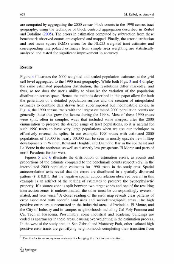
Results

Figure 4 illustrates the 2000 weighted and scaled population estimates at the grid

cell level aggregated to the 1990 tract geography. While both Figs. 3 and 4 display

the same estimated population distribution, the resolutions differ markedly, and

thus, so too does the user’s ability to visualize the variation of the population

distribution across space. Hence, the methods described in this paper allow for both

the generation of a detailed population surface and the creation of interpolated

estimates to combine data drawn from superimposed but incompatible zones. In

Fig. 4, the 1990 census tracts with the largest estimated 2000 population counts are

generally those that grew the fastest during the 1990s. Most of these 1990 tracts

were split, often in complex ways that included some merges, after the 2000

enumeration to preserve the desired range of tract populations, so it is natural for

such 1990 tracts to have very large populations when we use our technique to

effectively reverse the splits. In our example, 1990 tracts with estimated 2000

populations of 13,000 to nearly 30,000 can be seen in mostly upscale new hilltop

developments in Walnut, Rowland Heights, and Diamond Bar in the southeast and

La Verne in the northeast, as well as distinctly less prosperous El Monte and parts of

north Pasadena further west.

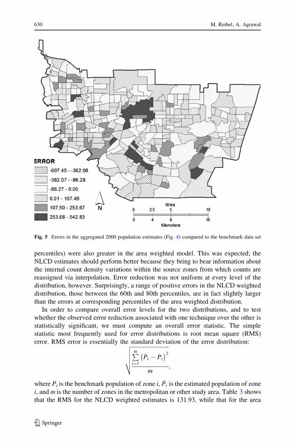
Figures 5 and 6 illustrate the distribution of estimation errors, as counts and

proportions of the estimate compared to the benchmark counts respectively, in the

interpolated 2000 population estimates for 1990 tracts in the study area. Spatial

autocorrelation tests reveal that the errors are distributed in a spatially dispersed

pattern (P £ 0.01). But the negative spatial autocorrelation observed overall in this

example is an artifact of the scaling of estimates to preserve the pycnophylactic

property. If a source zone is split between two target zones and one of the resulting

intersection zones is underestimated, the other must be correspondingly overesti-

mated, and vice versa.3 A closer reading of the error map reveals clear patterns of

error associated with specific land uses and sociodemographic areas. The high

positive errors are concentrated in the industrial areas of Irwindale, El Monte, and

the City of Industry and in campus neighborhoods including Cal Poly Pomona and

Cal Tech in Pasadena. Presumably, some industrial and academic buildings are

coded as apartments in these areas, causing overweighting in the estimation process.

In the west of the study area, in San Gabriel and Monterey Park, other isolated high

positive error tracts are gentrifying neighborhoods completing their transition from

3 Our thanks to an anonymous reviewer for bringing this fact to our attention.


123

mixed and heavily Hispanic to majority Chinese populations. In the process, many

larger houses are being built and inhabited by smaller households. The result is

overestimation of the population based on land cover weighting. In the far southeast

of the study area is another high positive error tract in upscale Diamond Bar. This

neighborhood is new development but it also has similar large homes and small

households, and is also heavily Asian, including many Chinese, Filipinos, and

Koreans.

High negative errors are found in poor, less densely built peripheral neighbor-

hoods that are overwhelmingly Hispanic and heavily populated by more recent

immigrants. Severe housing overcrowding in such areas, which include western

Pomona and parts of Hacienda Heights, La Puente, and Covina, creates much larger

actual populations than the weighting scheme estimates given the relatively low

density residential built environment.

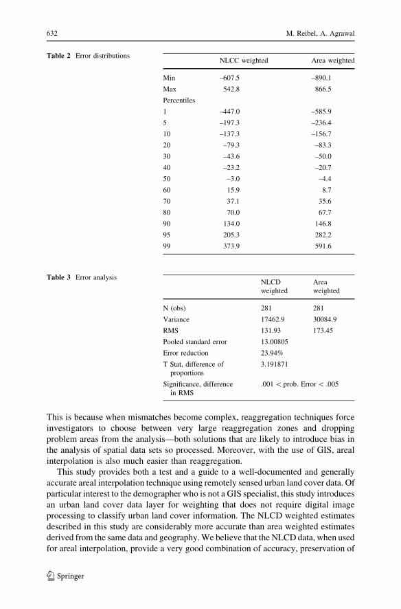
We can interpret from Table 2 that the error distributions for both the NLCD land

cover weighted estimates and the area weighted estimates are reasonably symmetrical

with means near zero, and that they correspond to approximate Gaussian normality.

Overall, the NLCD weighted distribution has fewer large errors in both the negative

and positive direction: the maximum and minimum error values are both greater in the

area weighted model and the error values at the extremes ([90th and \10th

Fig. 4 2000 population counts aggregated to the 1990 tract geography based on the population surfaceillustrated in Fig. 3. Note that natural breaks have been rounded to the nearest 100th value


123

percentiles) were also greater in the area weighted model. This was expected; the

NLCD estimates should perform better because they bring to bear information about

the internal count density variations within the source zones from which counts are

reassigned via interpolation. Error reduction was not uniform at every level of the

distribution, however. Surprisingly, a range of positive errors in the NLCD weighted

distribution, those between the 60th and 80th percentiles, are in fact slightly larger

than the errors at corresponding percentiles of the area weighted distribution.

In order to compare overall error levels for the two distributions, and to test

whether the observed error reduction associated with one technique over the other is

statistically significant, we must compute an overall error statistic. The simple

statistic most frequently used for error distributions is root mean square (RMS)

error. RMS error is essentially the standard deviation of the error distribution:ffiffiffiffiffiffiffiffiffiffiffiffiffiffiffiffiffiffiffiffiffiffiffiffiffiffiffiPmi¼1

P̂i � Pi

� �2

m

vuuut;

where Pi is the benchmark population of zone i, P̂i is the estimated population of zone

i, and m is the number of zones in the metropolitan or other study area. Table 3 shows

that the RMS for the NLCD weighted estimates is 131.93, while that for the area

Fig. 5 Errors in the aggregated 2000 population estimates (Fig. 4) compared to the benchmark data set


123

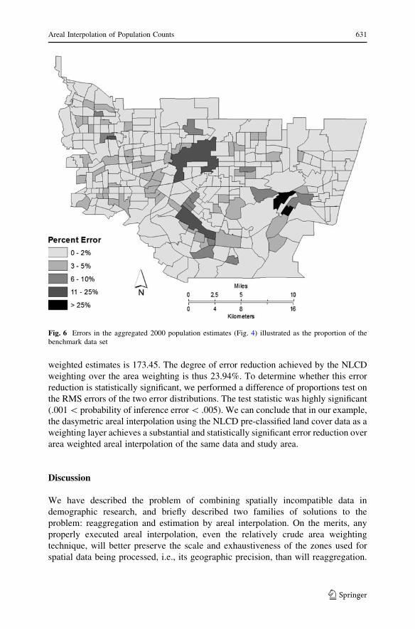
weighted estimates is 173.45. The degree of error reduction achieved by the NLCD

weighting over the area weighting is thus 23.94%. To determine whether this error

reduction is statistically significant, we performed a difference of proportions test on

the RMS errors of the two error distributions. The test statistic was highly significant

(.001 \ probability of inference error \ .005). We can conclude that in our example,

the dasymetric areal interpolation using the NLCD pre-classified land cover data as a

weighting layer achieves a substantial and statistically significant error reduction over

area weighted areal interpolation of the same data and study area.

Discussion

We have described the problem of combining spatially incompatible data in

demographic research, and briefly described two families of solutions to the

problem: reaggregation and estimation by areal interpolation. On the merits, any

properly executed areal interpolation, even the relatively crude area weighting

technique, will better preserve the scale and exhaustiveness of the zones used for

spatial data being processed, i.e., its geographic precision, than will reaggregation.

Fig. 6 Errors in the aggregated 2000 population estimates (Fig. 4) illustrated as the proportion of thebenchmark data set


123

This is because when mismatches become complex, reaggregation techniques force

investigators to choose between very large reaggregation zones and dropping

problem areas from the analysis—both solutions that are likely to introduce bias in

the analysis of spatial data sets so processed. Moreover, with the use of GIS, areal

interpolation is also much easier than reaggregation.

This study provides both a test and a guide to a well-documented and generally

accurate areal interpolation technique using remotely sensed urban land cover data. Of

particular interest to the demographer who is not a GIS specialist, this study introduces

an urban land cover data layer for weighting that does not require digital image

processing to classify urban land cover information. The NLCD weighted estimates

described in this study are considerably more accurate than area weighted estimates

derived from the same data and geography. We believe that the NLCD data, when used

for areal interpolation, provide a very good combination of accuracy, preservation of

Table 2 Error distributionsNLCC weighted Area weighted

Min –607.5 –890.1

Max 542.8 866.5

Percentiles

1 –447.0 –585.9

5 –197.3 –236.4

10 –137.3 –156.7

20 –79.3 –83.3

30 –43.6 –50.0

40 –23.2 –20.7

50 –3.0 –4.4

60 15.9 8.7

70 37.1 35.6

80 70.0 67.7

90 134.0 146.8

95 205.3 282.2

99 373.9 591.6

Table 3 Error analysisNLCD

weighted

Area

weighted

N (obs) 281 281

Variance 17462.9 30084.9

RMS 131.93 173.45

Pooled standard error 13.00805

Error reduction 23.94%

T Stat, difference of

proportions

3.191871

Significance, difference

in RMS

.001 \ prob. Error \ .005


123

data at appropriate scales, and ease of estimation. We hope that demographers will

consider areal interpolation when they are performing local and neighborhood analysis

that requires combining incompatible spatial data, and we recommend the NLCD

weighting approach described here. We also hope that the availability of GIS to help

solve difficult data processing problems will facilitate and help promote demographic

research on urban and spatial research questions in demography.

References

Bracken, I., & Martin, D. (1989). The generation of spatial population distributions from census centroid

data. Environment and Planning A, 21, 537–543.

Cockings, S., Fisher, P., & Langford, M. (1997). Parameterization and visualization of the errors in areal

interpolation. Geographical Analysis, 29(4), 314–328.

Eicher, C., & Brewer, C. (2001). Dasymetric mapping and areal interpolation: Implementation and

evaluation. Cartography and Geographic Information Science, 28, 125–138.

Fisher, P., & Langford, M. (1995). Modeling the errors in areal interpolation between zonal systems by

Monte Carlo simulation. Environment and Planning A, 27, 211–224.

Fisher, P., & Langford, M. (1996). Modeling sensitivity to accuracy in classified imagery. ProfessionalGeographer, 48, 299–309.

Flowerdew, R., & Green, M. (1989). Statistical methods for inference between incompatible zone

systems. In M. Goodchild, & S. Gopal (Eds.), The accuracy of spatial databases (pp. 239–247).

London, England: Taylor and Francis.

Flowerdew, R., & Green, M. (1992). Developments in areal interpolation methods and GIS. Annals ofRegional Science, 26, 67–78.

Goodchild, M., Anselin, L., & Deichmann, U. (1993). A framework for the areal interpolation of

socioeconomic data. Environment and Planning A, 25, 383–397.

Goodchild, M., & Lam, N. (1980). Areal interpolation: A variant of the traditional spatial problem. Geo-Processing, 1, 297–312.

Gotway, C., & Young, L. (2002). Combining incompatible data. Journal of the American StatisticalAssociation, 97, 632–648.

Jensen, J. R. (1996). Introductory digital image processing—A remote sensing perspective, 2nd ed. Upper

Saddle River NJ: Prentice Hall.

Langford, M., Maguire, D., & Unwin, D. (1991). The areal interpolation problem: Estimating population

using remote sensing in a GIS framework. In I. Masser, & M. Blakemore (Eds.), Handlinggeographic information: Methodology and potential applications (pp. 55–77). Harlow, Essex,

England: Longman.

Langford, M., & Unwin, D. (1994). Generating and mapping population density surfaces within a

geographical information system. Cartographic Journal, 31, 21–26.

Lillesand, T. M., & Kiefer, R. W. (1987). Remote sensing and image interpretation, 2nd ed. New York:

John Wiley and Sons.

Longley, P. A., Goodchild, M. F., Maguire, D. J., & Rhind, D. W. (2005). Geographic informationsystems and science, 2nd ed. New York: John Wiley & Sons.

Mennis, J. (2003). Generating surface models of population using dasymetric mapping. The ProfessionalGeographer, 55(1), 31–42.

Reibel, M. (2007). Geographic information systems and spatial data processing in demography: A review.

Population Research and Policy Review, 26(5–6). doi: 10.1007/s11113-007-9046-5.

Reibel, M., & Agrawal, A. (2005). Land use weighted areal interpolation. Proceedings of the GIS Planet

2005 International Conference, Estoril, Portugal.

Reibel, M., & Bufalino, M. E. (2005). A test of street weighted areal interpolation using geographic

information systems. Environment and Planning A, 37, 127–139.

Schowengerdt, R. A. (1997). Remote sensing: Models and methods for image processing, 2nd ed. San

Diego CA: Academic Press.

Tobler, W. (1979). Smooth pycnophylactic interpolation for geographical regions. Journal of theAmerican Statistical Association, 74, 519–536.


123

Areal Interpolation of Population Counts Using Pre-classified Land Cover Data

Documents

Transcript of Areal Interpolation of Population Counts Using Pre-classified Land Cover Data