Fundamenta Informaticae 32 (1997) 27-45 27IOS PressThe Topos of Labelled Trees:A Categorical Semantics for SCCSStefano KasangianDipartimento di Scienze dell'InformazioneUniversit�a Ca' Foscari di VeneziaVenezia, Italykasan@vmimat.mat.unimi.itSebastiano VignaDipartimento di Scienze dell'InformazioneUniversit�a degli Studi di MilanoMilano, Italyvigna@dsi.unimi.itAbstract. In this paper a we give a semantics for SCCS using the constructions of the topos oflabelled trees. The semantics accounts for all aspects of the original formulation of SCCS, in-cluding unbounded non-determinism. Then, a partial solution to the problem of characterizingbisimulation in terms of a class of morphisms is proposed. We de�ne a class of morphisms ofthe topos of trees, called con�ict preserving, such that two trees T and U are bisimilar iff thereis a pair of con�ict preserving morphisms f : T→ U and g : U→ T such that f g f = f andg f g = g. It is the �rst characterization which does not require the existence of a third quotientobject. The results can be easily extended to more general transition systems.Keywords: process algebras, semantics, category theory, topos theory1. IntroductionTrees and tree-like structures play an essential r�ole in the de�nition and in the study of the se-mantics of process algebras. In particular, when only �nite (or �nite-state) processes are con-sidered, trees have very manageable descriptions (such as, for instance, [5]).However, for the purpose of studying bisimulation related properties, domain theory providedthe tool of powerdomains based equations as a source of denotational objects. Domain theoryallows to exploit the concept of continuous map for the construction of suitable �xed point se-mantics.There are nonetheless some limitations (such as the cardinality of the branching degree) whichcall for a more powerful semantic domain, in which trees can be studied with the same ease as itwas possible for �nite state calculi, but in a generalized framework that lifts all restrictions on sizeand branching degree, although in a less constructive setting. Such a framework is provided bythe topos of labelled trees, a Grothendieck topos which arises naturally in the study of the functorcategory ω = Setωop . This category can be easily seen to be the category of forests; labellingcomes from the most important and studied source of new topoi, the slicing operation. Given an

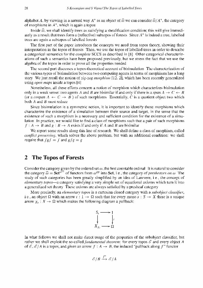
28 S.Kasangian and S.Vigna / The Topos of Labelled Treesalphabet A, by viewing in a natural way A∗ as an object of ω we can consider ω/A∗, the categoryof morphisms in A∗, which is again a toposInside ω, we shall identify trees as satisfying a shea��cation condition; this will give immedi-ately as a result that trees form a (re�ective) subtopos of forests. Since A∗ is indeed a tree, labelledtrees are again a subtopos of labelled forests.The �rst part of the paper introduces the concepts we need from topos theory, showing theirinterpretation in the topos of forests. Then, we use the topos of labelled trees in order to describea categorical semantics for the complete SCCS as described in [8]. Other categorical characteriz-ations of such a semantics have been proposed previously, but we stress the fact that we use thealgebra of the topos in order to prove all the properties needed.The second part discusses a topos-theoretical account of bisimulation. The characterization ofthe various types of bisimulation between two computing agents in terms of morphisms has a longstory. We just recall the notion of zig-zag morphism [12, 2], which has been recently generalizedusing open maps inside a topos [4].Nonetheless, all these efforts concern a notion of morphism which characterizes bisimulationonly in a weak sense: two agents A and B are bisimilar if and only if there is a span A→ C ← B(or a cospan A ← C → B ) of such morphisms. Essentially, C is a quotient object two whichboth A and B must reduce.Since bisimulation is a symmetric notion, it is important to identify those morphisms whichcharacterize the existence of a simulation between their source and target, in the sense that theexistence of such a morphism is a necessary and suf�cient condition for the existence of a simu-lation. In practice, we would like to �nd a class of morphisms such that a pair of such morphismsf : A→ B and g : B→ A exists if and only if A and B are bisimilar.We report some results along this line of research. We shall de�ne a class of morphism, calledcon�ict preserving, which solves the above problem, but with an additional condition: we shallrequire that f g f = f and g f g = g.2. The Topos of ForestsConsider the category given by the ordered setω, the �rst countable ordinal. It is natural to considerthe category ω = Setωop of functors from ωop into Set, i.e., the category of presheaves on ω. Thestudy of such categories has been greatly simpli�ed by an idea of Lawvere, i.e., the concept ofelementary topos�a category satisfying a very simple set of equational axioms which turn it intoa generalized set theory. These axioms are always satis�ed by a presheaf category.More precisely, an elementary topos is a cartesian closed category with a subobject classi�er,i.e., an object � with an arrow t : 1 → � such that for every mono s : S → X there is a uniquearrow χs : X → � which makes the following diagram a pullback:Ss //�� 1�� tXχs // �In what follows we shall not make direct usage of the properties of the subobject classi�er, butrather we shall exploit the so-called fundamental theorem: for every topos E and every object Aof E , E /A is a topos, and given an arrow f : A→ B, the induced �pullback along f � functorE /B f ∗−→ E /A

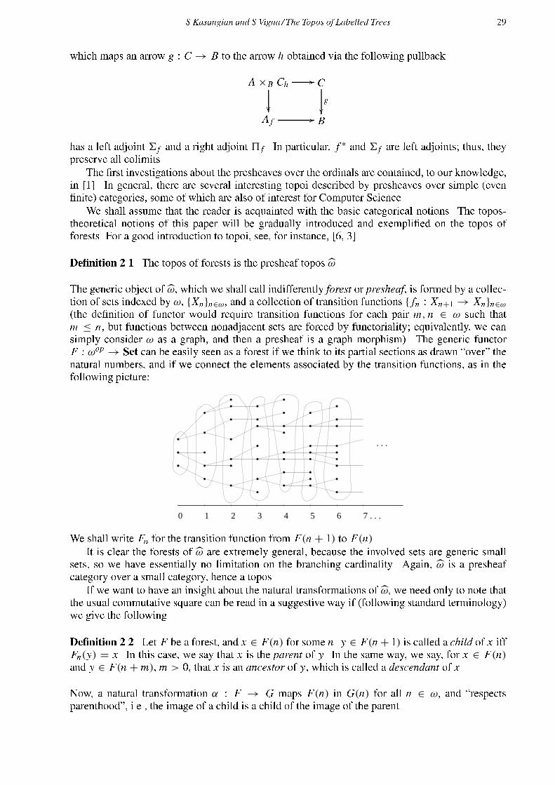
S.Kasangian and S.Vigna / The Topos of Labelled Trees 29which maps an arrow g : C → B to the arrow h obtained via the following pullbackA ×B Ch //�� C�� gA f // Bhas a left adjoint 6 f and a right adjoint 5 f . In particular, f ∗ and 6 f are left adjoints; thus, theypreserve all colimits.The �rst investigations about the presheaves over the ordinals are contained, to our knowledge,in [1]. In general, there are several interesting topoi described by presheaves over simple (even�nite) categories, some of which are also of interest for Computer Science.We shall assume that the reader is acquainted with the basic categorical notions. The topos-theoretical notions of this paper will be gradually introduced and exempli�ed on the topos offorests. For a good introduction to topoi, see, for instance, [6, 3].De�nition 2.1. The topos of forests is the presheaf topos ω.The generic object of ω, which we shall call indifferently forest or presheaf, is formed by a collec-tion of sets indexed by ω, {Xn}n∈ω, and a collection of transition functions { fn : Xn+1→ Xn}n∈ω(the de�nition of functor would require transition functions for each pair m, n ∈ ω such thatm ≤ n, but functions between nonadjacent sets are forced by functoriality; equivalently, we cansimply consider ω as a graph, and then a presheaf is a graph morphism). The generic functorF : ωop → Set can be easily seen as a forest if we think to its partial sections as drawn �over� thenatural numbers, and if we connect the elements associated by the transition functions, as in thefollowing picture:. . .

. . .

0 1 2 3 4 5 6 7We shall write Fn for the transition function from F(n + 1) to F(n).It is clear the forests of ω are extremely general, because the involved sets are generic smallsets, so we have essentially no limitation on the branching cardinality. Again, ω is a presheafcategory over a small category, hence a topos.If we want to have an insight about the natural transformations of ω, we need only to note thatthe usual commutative square can be read in a suggestive way if (following standard terminology)we give the followingDe�nition 2.2. Let F be a forest, and x ∈ F(n) for some n. y ∈ F(n+ 1) is called a child of x iffFn(y) = x . In this case, we say that x is the parent of y. In the same way, we say, for x ∈ F(n)and y ∈ F(n + m), m > 0, that x is an ancestor of y, which is called a descendant of x .Now, a natural transformation α : F → G maps F(n) in G(n) for all n ∈ ω, and �respectsparenthood�, i.e., the image of a child is a child of the image of the parent.

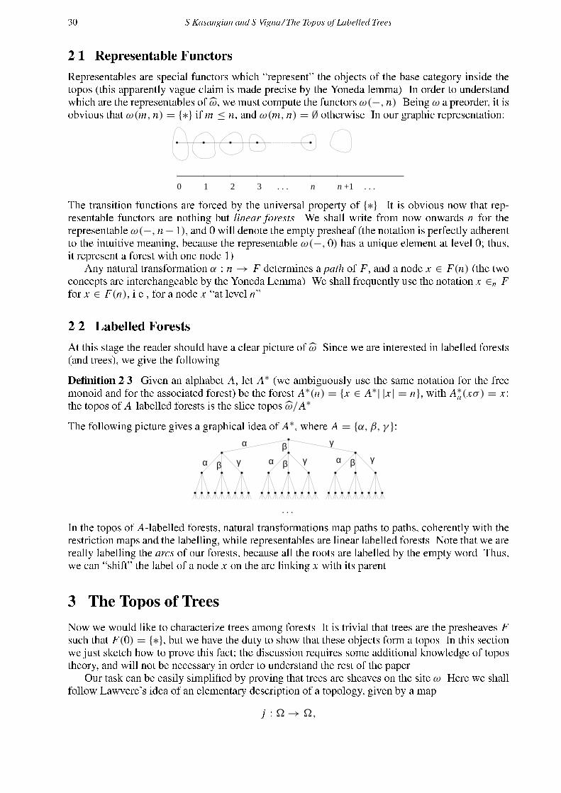
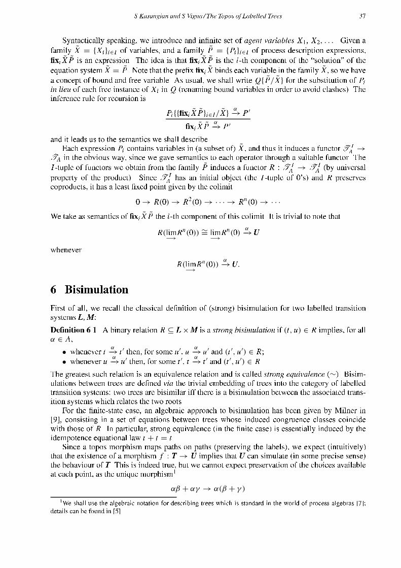
30 S.Kasangian and S.Vigna / The Topos of Labelled Trees2.1. Representable FunctorsRepresentables are special functors which �represent� the objects of the base category inside thetopos (this apparently vague claim is made precise by the Yoneda lemma). In order to understandwhich are the representables of ω, we must compute the functors ω(−, n). Being ω a preorder, it isobvious that ω(m, n) = {∗} if m ≤ n, and ω(m, n) = ∅ otherwise. In our graphic representation:. . .0 1 2 3 n n . . .+1The transition functions are forced by the universal property of {∗}. It is obvious now that rep-resentable functors are nothing but linear forests. We shall write from now onwards n for therepresentable ω(−, n−1), and 0 will denote the empty presheaf (the notation is perfectly adherentto the intuitive meaning, because the representable ω(−, 0) has a unique element at level 0; thus,it represent a forest with one node 1).Any natural transformation α : n → F determines a path of F, and a node x ∈ F(n) (the twoconcepts are interchangeable by the Yoneda Lemma). We shall frequently use the notation x ∈n Ffor x ∈ F(n), i.e., for a node x �at level n�.2.2. Labelled ForestsAt this stage the reader should have a clear picture of ω. Since we are interested in labelled forests(and trees), we give the followingDe�nition 2.3. Given an alphabet A, let A∗ (we ambiguously use the same notation for the freemonoid and for the associated forest) be the forest A∗(n) = {x ∈ A∗| |x | = n}, with A∗n(xσ) = x :the topos of A-labelled forests is the slice topos ω/A∗.The following picture gives a graphical idea of A∗, where A = {α, β, γ }:

α β γ α β γ α β γ

γ

. . .

α β

In the topos of A-labelled forests, natural transformations map paths to paths, coherently with therestriction maps and the labelling, while representables are linear labelled forests. Note that we arereally labelling the arcs of our forests, because all the roots are labelled by the empty word. Thus,we can �shift� the label of a node x on the arc linking x with its parent.3. The Topos of TreesNow we would like to characterize trees among forests. It is trivial that trees are the presheaves Fsuch that F(0) = {∗}, but we have the duty to show that these objects form a topos. In this sectionwe just sketch how to prove this fact; the discussion requires some additional knowledge of topostheory, and will not be necessary in order to understand the rest of the paper.Our task can be easily simpli�ed by proving that trees are sheaves on the site ω. Here we shallfollow Lawvere's idea of an elementary description of a topology, given by a mapj : �→ �,

S.Kasangian and S.Vigna / The Topos of Labelled Trees 31where � is the subobject classi�er, which satis�es certain axioms. In our case, it is not dif�cult tocheck that the map j de�ned on �(n) by 0 7→ 1, n 7→ n for n 6= 0 (we suppose that � is describedin the standard way, i.e., that �(n) is formed by the subobjects of the representable n+ 1) satis�esthe axioms, and thatProposition 3.1. The trees in ω are exactly the sheaves for j .This implies that trees form a re�ective subtoposT of the topos of forests. Moreover, since A∗ is asheaf, TA = T /A∗ is still a topos, and a re�ective subtopos of labelled forests. The shea��cationfunctor associated to j glues all the roots of a forest to a single point, as shown in the followingpicture:7→Note that this works also in the labelled case. We shall use T , U , . . . for unlabelled trees, and T,U, . . . for labelled trees, which are given by a morphism T ℓT

−→ A∗.4. Special PropertiesWe shall now show some special factorization properties of the topos of trees T which we shalluse in what follows. We start by introducing some operations.It is known that a sheaf topos is cocomplete, and that colimits are computed as the associatedsheaf of the pointwise colimit presheaf. In particular we have all coproducts. We shall denotewith T + U the coproduct T ∐U , and we shall write ∑i∈I Ti for ∐i∈I Ti . This operation isparticularly important from the computer science point of view, because it will be used to representthe nondeterministic sum of the process represented by T and U . If we sum two forests F, G theresult is as follows:Π

=F G F GSince the coproduct of two sheaf is given be sheaf associated to the coproduct in the presheafcategory, the coproduct in T identi�es the roots of two trees T,U , as in the following picture:

Π

=T UUTThus, the operation of summing to forests is just a �placing side by side�, while summing two trees(in the tree topos) glues roots. However, �placing� does not denote in any sense a non-commutative(order-inducing) operation.The other operation we want to introduce is the categorical version of Milner's left-pre�x [7, 10,13]. It is an endofunctor of T , which we shall denote with S, whose intuitive effect is representedin the following picture:

T

S7→

TThe formalization of this process is very simple: we want to shift by one position every section,and then set T (0) = {∗}. This leads to the following

32 S.Kasangian and S.Vigna / The Topos of Labelled TreesDe�nition 4.1. The shift functor S : T → T is de�ned on objects byS(T )(n) = T (n − 1) for n > 0S(T )(0) = {∗}Given by a natural transformation α : T → U , S(α) has componentsS(α)(n) = α(n − 1) for n > 0S(α)(0) = ! : {∗} → {∗}In the labelled case, we have to de�ne a whole class of shift functors indexed by the labellingalphabet A. The de�nition is obvious, and the details are left to the reader. We shall denote simplywith α the shift functor adding an α-labelled arc, for each α ∈ A.4.1. Unique DecompositionProposition 4.1. Every tree T ∈ T has an essentially unique normal formT ∼=∑i∈I S(Ti)for a set of indices I and of trees Ti , unique up to isomorphism (in Set and T , respectively).Proof:De�ne I = T (1) and Ti(n) inductively byTi(0) = {x ∈ T (1) | T0(x) = i}Ti(n) = {x ∈ T (n + 1) | Tn(x) ∈ Ti(n − 1)} for n > 0The restrictions are de�ned in the obvious way. It is trivial to show that T ∼=∑i∈I S(Ti).In the labelled case, this proposition becomes the fundamental and well-known unique decompos-ition theorem:Theorem 4.1. Every tree T ∈ TA has an essentially unique normal formT ∼=∑i∈I αi(Ti),where αi ∈ A, for a set of indices I and of trees Ti , unique up to isomorphism (in Set and TA,respectively).4.2. Inductive Form of the ProductWe shall prove now some properties which will be useful in order to write the product of ω in aninductive form.Proposition 4.2. S preserves products, i.e.,S(T × U) ∼= S(T )× S(U).Proof:At level 0 we have trivially {∗} × {∗} ∼= {∗}. At level n > 0 we haveS(T × U)(n) = (T × U)(n − 1)∼= T (n − 1)× U(n − 1)∼= S(T )(n)× S(U)(n)and analogously for the transition functions.

S.Kasangian and S.Vigna / The Topos of Labelled Trees 33The following proposition is obvious by left adjointness of (−)× X :Proposition 4.3. In ω �nite products distribute over arbitrary sums, i.e.,( ∑i∈I Ti)× U ∼= ( ∑i∈I Ti × U)

.Now we can describe the product of two trees in an inductive form:Proposition 4.4. For each pair of trees T =∑i∈I S(Ti), U =∑j∈J S(Uj ), the product T × U isgiven by T × U ∼= ∑

(i, j)∈I×J S(Ti × Uj )Proof: T × U ∼=∑i∈I S(Ti)×∑j∈J S(Uj )

∼=∑i∈I (S(Ti)×∑j∈J S(Uj ))

∼=∑i∈I ∑j∈J (S(Ti)× S(Uj ))

∼=∑i∈I ∑j∈J (S(Ti × Uj ))

∼=∑

(i, j)∈I×J S(Ti × Uj ).4.3. The �Parent of� MapFor any tree T , there is an associated subobject latticeP(T ) formed in a standard way by equi-valence classes of monos into T . It is characteristic of any topos thatP(T ) has intersections andunions; however, in the topos of trees there is also an endomap π :P(T )→P(T ) which re�ectsthe �parent of� relation induced by the restrictions. In order to de�ne π , we point out that anysubobject U of T can be written as a union of singletons ⋃xi∈ni T {xi}, where {xi ∈n i T }i∈I is anindexed family of elements (nodes) of T .De�nition 4.2. The map π is de�ned on U =⋃xi∈ni T {xi} ⊆ T byπ(U) =

⋃xi∈ni T{Tn i−1xi},where T−1 = 1T (0).By de�nition, π preserves all the sups and the infs existing in P(T ). Intuitively, π �eats� onelevel of leaves each time it is applied. In the following example, the subtree U is represented bythe continuous lines, and the nodes which π will remove have been marked:π7→

34 S.Kasangian and S.Vigna / The Topos of Labelled Trees5. A Categorical Semantics for SCCSWe are now going to exhibit a semantics for SCCS which uses the topos constructions we justdescribed. It was surprising for the authors to discover the strict relation between the SCCS oper-ational semantics and the properties of the topos. For instance, a crucial decision taken in SCCS isto allow in�nitary (small set indexed) sums but only �nite products. It turns out that this is exactlycorresponding to the fact that only �nite limits commute with �ltered colimits in Set, while anysum has this property (being a left adjoint).We shall introduce the SCCS constructors and discuss their topos-theoretical analogues. Notethat since in the previous sections we discussed just non-labelled constructions, we shall graduallyintroduce their labelled counterparts.The basic assumption of SCCS is that there is an abelian group Act = 〈A,2, 1, ( )〉 of actions(the reasons for such a choice are thoroughly discussed in [8]). We shall work from now onwardsin the topos of trees labelled in A, and we shall write 2 also for the lifting to A∗ of the groupproduct; in particular, 2n : A∗(n)× A∗(n)→ A∗(n) is de�ned by〈〈α1, α2, . . . , αn〉, 〈β1, β2, . . . , βn〉〉 7→ 〈α12β1, α22β2, . . . , αn2βn〉.The operational semantics of SCCS will be presented, as usual, in SOS form [11]. We shall strictlyfollow [8], where more details can be found.We must have a way of proving that the operational semantics is preserved by our tree se-mantics. Thus, we have to de�ne what does it mean to have a derivation of a tree.De�nition 5.1. Given a labelled tree T = T ℓT

−→ A∗, T α−→T′ iff T = α(T′)+U for some U.Since we know that T =∑i∈I αi(Ti) in an essentially unique way, the derivations of T are all andonly the derivations T αi

−→ Ti . The constant 0 of SCCS (the process which can perform no action)corresponds here to the tree 1 (the representable tree with just one node).5.1. Pre�xingFor any action α ∈ A, it is possible to pre�x a process description P with α, getting the newdescription α.P. The inference rule is thenα.P α−→ P.It is straightforward to see that the shift functors allows us to give semantics to α.. By uniquedecomposition,

α(T)α−→T.It is not dif�cult to show that α(−) preserves �ltered colimits; indeed, if lim

−→Ti = T for a �lteredfamily {Ti}i∈I , with injections µi : Ti → T, the natural transformations α(µi) : α(Ti) → α(T)induce a transformation lim

−→α(Ti)→ α(T) which can be easily proved to be an isomorphism by asectionwise argument; we leave the details to the reader.5.2. SummationFor any (possibly in�nite) family of processes {Pi}i∈I , ∑i∈I Pi is a process. The inference rule isPi α

−→ P∑i∈I Pi α

−→ P .

S.Kasangian and S.Vigna / The Topos of Labelled Trees 35The summation of processes is exactly matched by the summation (coproduct) in the topos TA.The empty sum is of course the initial object, which is the root-only tree. Note that since summa-tion is a left adjoint, it preserves all colimits. By unique decomposition, if Ti = ∑j∈Ji αi j (Ti j )then ∑i∈I Ti = ∑

( j,i)∈∑i∈I Ji αi j (Ti j ).Thus, any derivation Ti αi j−→ Ti j induces a derivation ∑i∈I Ti αi j

−→ Ti j .5.3. ProductThe (parallel composition) product of two processes is probably the most remarkable operator ofSCCS, both because of its �non-interleaving� nature and of its radical departure from CCS in notallowing a single action of one of the processes to happen if not in correspondence to an action ofthe other process. Indeed, the inference ruleP α−→ P ′ Q β

−→ Q′P × Q α2β−−→ P ′ × Q′shows that, for instance, α.β.0×γ.0 has the same behaviour as (α2γ ).0 (i.e., the information about

β is lost). However, it is exactly this feature that maps so elegantly the SCCS parallel constructorinto the topos.We start by describing the tensor product that we shall use for the semantics of the parallelcomposition. Since in SCCS synchronization is accomplished by allowing any possible pair ofaction to happen (via the composition operator 2), we take the product of the non-labelled treesand then we compose their labelling arrows with 2.De�nition 5.2. Given two labelled trees T = T ℓT−→ A∗, U = U ℓU

−→ A∗, the tensor product T⊗Uis de�ned as T × U ℓT×ℓU−−−−→ A∗ × A∗ 2

−→ A∗on the objects, and as f ⊗ f ′ = f × f ′on arrows f : T→ U, f ′ : T′→ U′.Note that the de�nition of the tensor of two arrows is indeed correct:2 ◦ (ℓT ′ × ℓU ′) ◦ ( f × f ′) = 2 ◦ (ℓT ′ ◦ f × ℓU ′ ◦ f ′) = 2 ◦ (ℓT × ℓU).It is now easy to apply Proposition 4.4, thus obtaining the followingProposition 5.1. Let T =∑i∈I αi(Ti), U =∑j∈J βj (Uj ); we haveT⊗ U ∼= ∑

(i, j)∈I×J(αi2βj )(Ti ⊗ Uj ).It is immediate from this result to show thatT⊗ U αi2βj−−−→ Ti ⊗ Ujwhenever T αi

−→ Ti and U βj−→ Uj . An essential property is thatProposition 5.2. The tensor product ⊗ preserves �ltered colimits (in both entries).This is a natural consequence of the fact that ⊗ is �essentially� a product, �nite products com-mute with �ltered colimits in Set and the associated sheaf functor preserves all colimits and �niteproducts. The proof goes exactly like the proof for Set, just noticing that the way the isomorphismis built implies that it commutes with the labelling morphisms.

36 S.Kasangian and S.Vigna / The Topos of Labelled Trees5.4. RestrictionRestriction allows to restrict the behaviour of a process to a certain subset of B of A containing 1.Its inference rule is P α−→ P ′P\B α−→ P ′\B (α ∈ B).The injection j : B → A induces a triple of functors j∗, 6j and 5j . The effect of j∗ is exactlyto cut from a tree any subtrees starting with a branch whose label is not in B. Then 6j can takeus back to our labelled topos by seeing a tree labelled on B as a tree labelled on A. Thus, thesemantics of restriction is σj ◦ j∗. By looking at the pullback diagram which de�nes j∗, one cansee that j∗(α(T)) = α( j∗(T)), if α ∈ B, but j∗(α(T)) = 0 if α 6∈ B. Thus,j∗(T) = j∗( ∑i∈I αi(Ti)) =∑i∈L αi( j∗(Ti)),where L = {i ∈ I | αi ∈ B}. But then j∗(T)

α−→ j∗(Ti)iff αi ∈ B.Note that both 6j and j∗ are left adjoints: this means that also their composition is a leftadjoint, and thus preserves all colimits.5.5. RelabellingRelabelling allows to change the name of the actions of a process. It is useful in order to generatedifferent copies of a process, or to express non �nite-state systems (even with �nite recursion). Itsinference rule P α−→ P ′

ϕ[P] ϕ(α)−−→ ϕ[P ′]depends on a group morphism ϕ : Act → Act. This operator is (under reasonable assumptions)derivable from the other ones (as shown, again, in [8]). However, its topos semantics is verysimple: ϕ induces the usual triple of functors ϕ∗, 6ϕ and 5ϕ . In this case, 6ϕ provides us withthe semantics of relabelling (remember that 6ϕ is just �composition with ϕ�, which is exactlyrelabelling). Indeed, it is straightforward to show that

6ϕ(T) =∑i∈I ϕ(αi)(6ϕ(Ti)),which implies

6ϕ(T)ϕ(αi )−−−→ 6ϕ(Ti).5.6. RecursionThe most relevant application of topos theory is that we do not have to prove anything aboutrecursion. As we noted in each of the previous sections, �general abstract nonsense� allowed usto prove that each operator commuted with (preserved) �ltered colimits. Since we are going tobuild the semantics of an equation system via a �ltered colimit, we have for free existence anduniqueness of minimal �xed point solutions.

S.Kasangian and S.Vigna / The Topos of Labelled Trees 37Syntactically speaking, we introduce and in�nite set of agent variables X1, X2, . . . . Given afamily X = {Xi}i∈I of variables, and a family P = {Pi}i∈I of process description expressions,�xi X P is an expression. The idea is that �xi X P is the i-th component of the �solution� of theequation system X = P. Note that the pre�x �xi X binds each variable in the family X , so we havea concept of bound and free variable. As usual, we shall write Q{ P/ X} for the substitution of Piin lieu of each free instance of Xi in Q (renaming bound variables in order to avoid clashes). Theinference rule for recursion is Pi{{�xi X P}i∈I/ X} α−→ P ′�xi X P α

−→ P ′and it leads us to the semantics we shall describe.Each expression Pi contains variables in (a subset of) X , and thus it induces a functor T IA →TA in the obvious way, since we gave semantics to each operator through a suitable functor. TheI -tuple of functors we obtain from the family P induces a functor R : T IA → T IA (by universalproperty of the product). Since T IA has an initial object (the I -tuple of 0's) and R preservescoproducts, it has a least �xed point given by the colimit0→ R(0)→ R2(0)→ · · · → Rn(0)→ · · ·We take as semantics of �xi X P the i-th component of this colimit. It is trivial to note thatR(lim−→

Rn(0)) ∼= lim−→

Rn(0) α−→Uwhenever R(lim

−→Rn(0)) α

−→U.6. BisimulationFirst of all, we recall the classical de�nition of (strong) bisimulation for two labelled transitionsystems L,M:De�nition 6.1. A binary relation R ⊆ L×M is a strong bisimulation if (t, u) ∈ R implies, for allα ∈ A,• whenever t α

−→ t ′ then, for some u′, u α−→ u′ and (t ′, u′) ∈ R;

• whenever u α−→u′ then, for some t ′, t α

−→ t ′ and (t ′, u′) ∈ R.The greatest such relation is an equivalence relation and is called strong equivalence (∼). Bisim-ulations between trees are de�ned via the trivial embedding of trees into the category of labelledtransition systems: two trees are bisimilar iff there is a bisimulation between the associated trans-ition systems which relates the two roots.For the �nite-state case, an algebraic approach to bisimulation has been given by Milner in[9], consisting in a set of equations between trees whose induced congruence classes coincidewith those of R. In particular, strong equivalence (in the �nite case) is essentially induced by theidempotence equational law t + t = t .Since a topos morphism maps paths on paths (preserving the labels), we expect (intuitively)that the existence of a morphism f : T → U implies that U can simulate (in some precise sense)the behaviour of T. This is indeed true, but we cannot expect preservation of the choices availableat each point, as the unique morphism1αβ + αγ → α(β + γ )1We shall use the algebraic notation for describing trees which is standard in the world of process algebras [7];details can be found in [5].

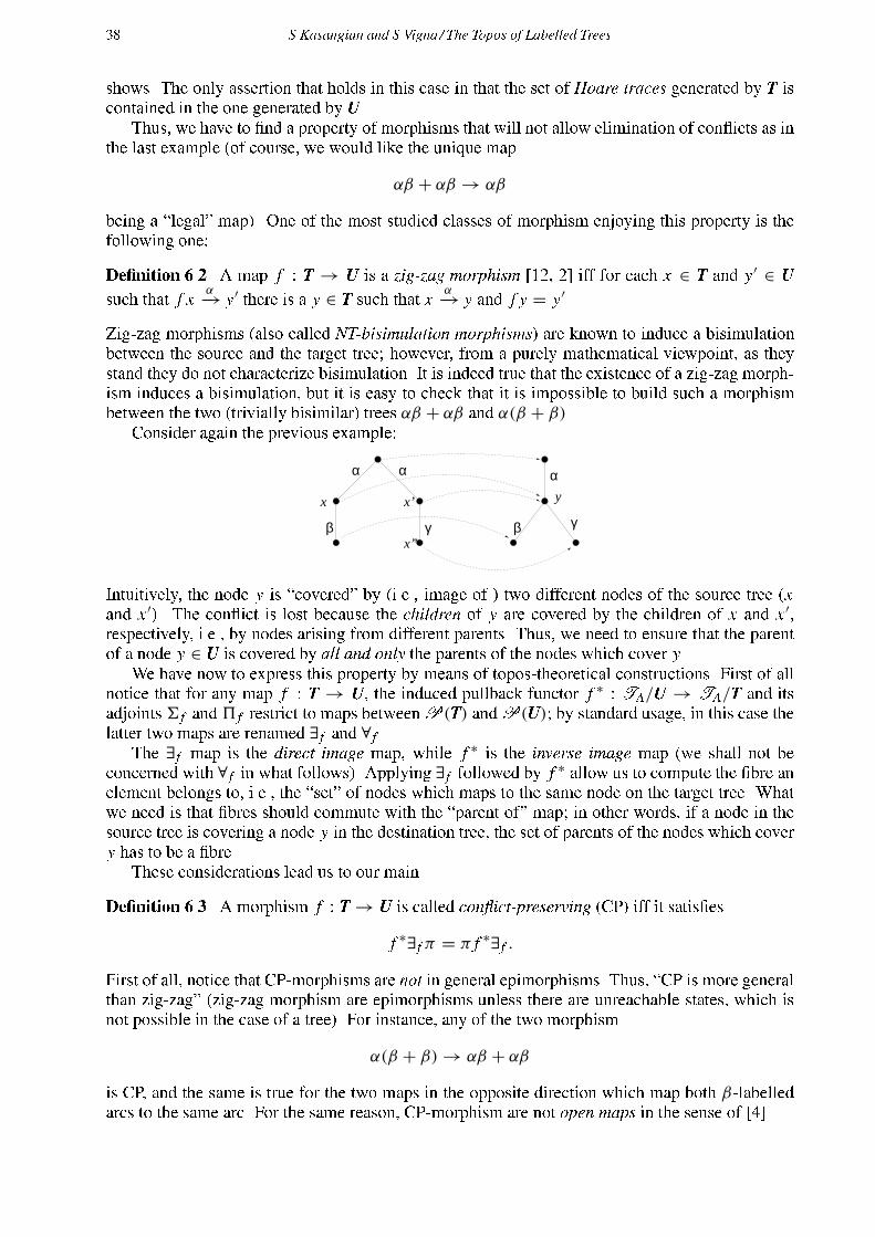
38 S.Kasangian and S.Vigna / The Topos of Labelled Treesshows. The only assertion that holds in this case in that the set of Hoare traces generated by T iscontained in the one generated by U.Thus, we have to �nd a property of morphisms that will not allow elimination of con�icts as inthe last example (of course, we would like the unique mapαβ + αβ → αβbeing a �legal� map). One of the most studied classes of morphism enjoying this property is thefollowing one:De�nition 6.2. A map f : T → U is a zig-zag morphism [12, 2] iff for each x ∈ T and y ′ ∈ Usuch that f x α

−→ y′ there is a y ∈ T such that x α−→ y and f y = y′.Zig-zag morphisms (also called NT-bisimulation morphisms) are known to induce a bisimulationbetween the source and the target tree; however, from a purely mathematical viewpoint, as theystand they do not characterize bisimulation. It is indeed true that the existence of a zig-zag morph-ism induces a bisimulation, but it is easy to check that it is impossible to build such a morphismbetween the two (trivially bisimilar) trees αβ + αβ and α(β + β).Consider again the previous example:

’x’

α

x x’

α

γβ

y

α

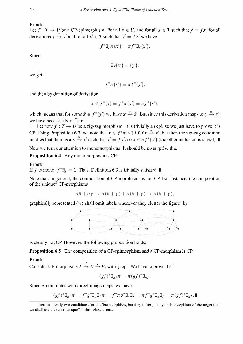
β γIntuitively, the node y is �covered� by (i.e., image of ) two different nodes of the source tree (xand x ′). The con�ict is lost because the children of y are covered by the children of x and x ′,respectively, i.e., by nodes arising from different parents. Thus, we need to ensure that the parentof a node y ∈ U is covered by all and only the parents of the nodes which cover y.We have now to express this property by means of topos-theoretical constructions. First of allnotice that for any map f : T → U, the induced pullback functor f ∗ : TA/U → TA/T and itsadjoints 6 f and 5 f restrict to maps betweenP(T) andP(U); by standard usage, in this case thelatter two maps are renamed ∃ f and ∀ f .The ∃ f map is the direct image map, while f ∗ is the inverse image map (we shall not beconcerned with ∀ f in what follows). Applying ∃ f followed by f ∗ allow us to compute the �bre anelement belongs to, i.e., the �set� of nodes which maps to the same node on the target tree. Whatwe need is that �bres should commute with the �parent of� map; in other words, if a node in thesource tree is covering a node y in the destination tree, the set of parents of the nodes which covery has to be a �bre.These considerations lead us to our mainDe�nition 6.3. A morphism f : T→ U is called con�ict-preserving (CP) iff it satis�esf ∗∃ f π = π f ∗∃ f .First of all, notice that CP-morphisms are not in general epimorphisms. Thus, �CP is more generalthan zig-zag� (zig-zag morphism are epimorphisms unless there are unreachable states, which isnot possible in the case of a tree). For instance, any of the two morphismα(β + β)→ αβ + αβis CP, and the same is true for the two maps in the opposite direction which map both β-labelledarcs to the same arc. For the same reason, CP-morphism are not open maps in the sense of [4].

S.Kasangian and S.Vigna / The Topos of Labelled Trees 39What is not allowed by CP-morphisms is partial glueing of paths. For instance, the unique mapf : αβ + αγ → α(β + γ )is not CP because (using the notation of the previous �gure){x ′} = π f ∗∃ f {x ′′} = π{x ′′} 6= f ∗∃ f π{x ′′} = {x, x ′}.The following proposition makes some characterizations of CP-morphisms explicit:Proposition 6.1. Given a morphism f : T→ U, the following conditions are equivalent:

• f ∗∃ f π = π f ∗∃ f ;• f ∗π∃ f = π f ∗∃ f ;• f ∗∃ f π ≤ π f ∗∃ f ;• f ∗π∃ f ≤ π f ∗∃ f .Proof:The �rst two conditions are obviously equivalent, because π and direct image maps commute.Moreover, since π f ∗ ≤ f ∗π , the last two conditions are suf�cient for establishing the �rst two.Note that up to now we discussed con�ict preservation using singletons, while the condition statedin De�nition 6.3 is quanti�ed over all subsets of T. This however is not a problem because of thefollowingProposition 6.2. Given a morphism f : T→ Uf ∗∃ f π = π f ∗∃ f iff ∀y ∈ U f ∗∃ f π{y} = π f ∗∃ f {y}.Proof:One implication is obvious. Moreover, since f ∗ and ∃ f are left adjoints, they preserve all sups, sofor any V =⋃xi∈niV{xi} ⊆ T we havef ∗∃ f π ⋃xi∈niT{xi} = f ∗∃ f ⋃xi∈niTπ{xi} = ⋃xi∈niT f ∗∃ f π{xi} =

⋃xi∈ni Tπ f ∗∃ f {xi} = π f ∗∃ f ⋃xi∈niT{xi}.Note moreover that CP-epimorphisms enjoy a slight simpli�cation of the CP condition:Proposition 6.3. An epimorphism f : T → U is CP iff f ∗π = π f ∗ iff ∀x ∈ T f ∗π{x} =π f ∗{x}.Proof:By Proposition 6.1, f is CP iff

∀x ∈ T f ∗π∃ f {x} = π f ∗∃ f {x},and since f is epimorphic, this is equivalent to∀y ∈ U f ∗π{y} = π f ∗{y}.A �rst insight about CP-morphisms comes from the followingTheorem 6.1. A morphism is zig-zag iff it is a CP-epimorphism.

40 S.Kasangian and S.Vigna / The Topos of Labelled TreesProof:Let f : T→ U be a CP-epimorphism. For all y ∈ U, and for all x ∈ T such that y = f x , for allderivations y α−→ y′ and for all x ′ ∈ T such that y′ = f x ′ we havef ∗∃ f π{x ′} = π f ∗∃ f {x ′}.Since

∃ f {x ′} = {y′},we get f ∗π{y′} = π f ∗{y′},and then by de�nition of derivationx ∈ f ∗{y} = f ∗π{y′} = π f ∗{y′},which means that for some x ∈ f ∗{y′} we have x σ−→ x . But since this derivation maps to y α

−→ y′,we have necessarily x α−→ x .Let now f : T→ U be a zig-zag morphism. It is trivially an epi, so we just have to prove it isCP. Using Proposition 6.3, we note that x ∈ f ∗π{y′} iff f x α

−→ y′; but then the zig-zag conditionimplies that there is a x α−→ x ′ such that y′ = f x ′, so x ∈ π f ∗{y′} (the other inclusion is trivial).Now we turn our attention to monomorphisms. It should be no surprise thatProposition 6.4. Any monomorphism is CP.Proof:If f is mono, f ∗∃ f = 1. Thus, De�nition 6.3 is trivially satis�ed.Note that, in general, the composition of CP-morphisms is not CP. For instance, the compositionof the unique2 CP-morphismsαβ + αγ → α(β + γ )+ α(β + γ )→ α(β + γ ),graphically represented (we shall omit labels whenever they clutter the �gure) by

is clearly not CP. However, the following proposition holds:Proposition 6.5. The composition of a CP-epimorphism and a CP-morphism is CP.Proof:Consider CP-morphisms T f−→ U g

−→V, with f epi. We have to prove that(g f )∗∃g f π = π(g f )∗∃g f .Since π commutes with direct image maps, we have

(g f )∗∃g f π = f ∗g∗∃g∃ f π = f ∗πg∗∃g∃ f = π f ∗g∗∃g∃ f = π(g f )∗∃g f .2There are really two candidates for the �rst morphism, but they differ just by an isomorphism of the target tree;we shall use the term �unique� in this relaxed sense.

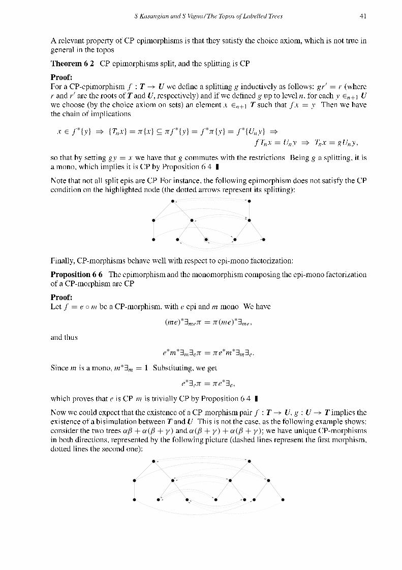
S.Kasangian and S.Vigna / The Topos of Labelled Trees 41A relevant property of CP-epimorphisms is that they satisfy the choice axiom, which is not true ingeneral in the topos.Theorem 6.2. CP-epimorphisms split, and the splitting is CP.Proof:For a CP-epimorphism f : T→ U we de�ne a splitting g inductively as follows: gr ′ = r (wherer and r ′ are the roots of T and U, respectively) and if we de�ned g up to level n, for each y ∈n+1 Uwe choose (by the choice axiom on sets) an element x ∈n+1 T such that f x = y. Then we havethe chain of implicationsx ∈ f ∗{y} ⇒ {Tnx} = π{x} ⊆ π f ∗{y} = f ∗π{y} = f ∗{Un y} ⇒f Tnx = Un y ⇒ Tnx = gUn y,so that by setting gy = x we have that g commutes with the restrictions. Being g a splitting, it isa mono, which implies it is CP by Proposition 6.4.Note that not all split epis are CP. For instance, the following epimorphism does not satisfy the CPcondition on the highlighted node (the dotted arrows represent its splitting):Finally, CP-morphisms behave well with respect to epi-mono factorization:Proposition 6.6. The epimorphism and the monomorphism composing the epi-mono factorizationof a CP-morphism are CP.Proof:Let f = e ◦ m be a CP-morphism, with e epi and m mono. We have

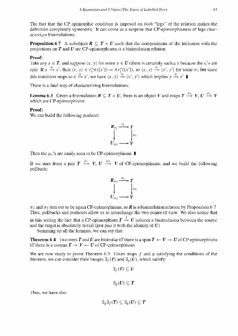
(me)∗∃meπ = π(me)∗∃me,and thus e∗m∗∃m∃eπ = πe∗m∗∃m∃e.Since m is a mono, m∗∃m = 1. Substituting, we gete∗∃eπ = πe∗∃e,which proves that e is CP. m is trivially CP by Proposition 6.4.Nowwe could expect that the existence of a CP-morphism pair f : T→ U, g : U→ T implies theexistence of a bisimulation between T and U. This is not the case, as the following example shows:consider the two trees αβ + α(β + γ ) and α(β + γ )+ α(β + γ ); we have unique CP-morphismsin both directions, represented by the following picture (dashed lines represent the �rst morphism,dotted lines the second one):

42 S.Kasangian and S.Vigna / The Topos of Labelled Treeshowever, the two trees are trivially not bisimilar.Indeed, we need a (possibly equational) condition on f and g that states that they are �compat-ible� in some suitable sense. This leads to our mainTheorem 6.3. T ∼ U iff there is a pair of CP-morphisms T f−→U g

−→T such thatf g f = f g f g = g.The proof of the theorem requires a couple of lemmata which are interesting in their own right.They use pullbacks and pushouts in order to relate at a categorical level pairs of maps into a thirdobject and bisimulation relations. Note that some of the claims which concern CP-epimorphismsare already known from the theory of zig-zag morphisms; we restate them in our setting in orderto make the treatment self-contained.Consider a bisimulation R between T and U; if we follow strictly De�nition 6.1, we are forcedto forget the topos structure and to consider simply a subset of ∑n T(n) ×∑n U(n), because theproduct of T and U in the labelled topos is given by the pullbackT ×A∗ U�� // T�� ℓTUℓU // A∗which does not contain (at the set-theoretical level) all the possible node pairs. However, it doescontain all those node pairs which one can get to via paths labelled identically; these ones are theonly pairs which are relevant when proving that two trees are bisimilar (which means that theirroot are bisimilar for some bisimulation R). This intuition is formalized by the followingLemma 6.1. Given a bisimulation R between T and U, the subobject R of T× U de�ned byR = {〈x, y〉 ∈ T× U | 〈x, y〉 ∈ R}is still a bisimulation.Proof:Of course, calling the roots of T and U respectively r and r ′, 〈r, r ′〉 ∈ R; but since r ∈ε T andr ′ ∈ε U, we have 〈r, r ′〉 ∈ε R. Now, given 〈x, x ′〉 ∈s R, for each derivation x α

−→ y there is aderivation x ′ α−→ y′ such that 〈y, y′〉 ∈ R. But y ∈sα T and y′ ∈sα U, so 〈y, y′〉 ∈sα R.In other words, if we restrict a bisimulation between two trees to the pairs of nodes living on thesame partial section, we still have a bisimulation relation. The extra information is not relevantfor establishing the bisimilarity of the trees. From now onwards, we shall denote by the topossubobject R ⊆ T× U a generic bisimulation between T and U.By the universal property of the product, each bisimulation R has two associated maps R r1

−→ Tand R r2−→ U; this maps, of course, are not arbitrary.Lemma 6.2. Given a bisimulation R ⊆ T× U, the associated maps r1, r2 are CP-epimorphisms.Proof:By induction, R is a total relation; thus, the maps r1 and r2 are epimorphisms. We have to showthat the equations r∗i π = πr∗i hold (i = 1, 2). Let us write down explicitly the meaning of the twosides of these equations. For all x ′ ∈ T and 〈x, y〉 ∈ R

〈x, y〉 ∈ r∗1π({x ′}) ⇐⇒ r1〈x, y〉 ∈ π({x ′}) ⇐⇒ x α−→ x ′ for some α

〈x, y〉 ∈ πr∗1 ({x ′}) ⇐⇒ 〈x, y〉 α−→〈x ′, y′〉 for some α and some y′,and analogously for U. Now, if 〈x, y〉 ∈ R, x ′ ∈ T and x α

−→ x ′, by de�nition of bisimulationy α−→ y′ and 〈x ′, y′〉 ∈ R, so 〈x, y〉 α

−→〈x ′, y′〉. Thus, r∗i π ⊆ πr∗i . The other inclusion is trivial.

S.Kasangian and S.Vigna / The Topos of Labelled Trees 43The fact that the CP-epimorphic condition is imposed on both �legs� of the relation makes thede�nition completely symmetric. It can come as a surprise that CP-epimorphicness of legs char-acterizes bisimulations:Proposition 6.7. A subobject R ⊆ T × U such that the compositions of the inclusion with theprojections on T and U are CP-epimorphisms is a bisimulation relation.Proof:Take any x ∈ T, and suppose 〈x, y〉 for some y ∈ U (there is certainly such a y because the ri 's areepi). If x α−→ x ′, then 〈x, y〉 ∈ r∗1π({x ′}) = πr∗1 ({x ′}), so 〈x, y〉 σ

−→ 〈x ′, y′〉 for some σ ; but sincethis transition maps to x α−→ x ′, we have 〈x, y〉 α

−→〈x ′, y′〉 which implies y α−→ y′.There is a dual way of characterizing bisimulations:Lemma 6.3. Given a bisimulation R ⊆ T × U, there is an object V and maps T µ1

−→ V, U µ2−→ Vwhich are CP-epimorphisms.Proof:We can build the following pushout: Rr2 //r1�� T�� µ1Uµ2 // VThen the µi 's are easily seen to be CP-epimorphisms.If we start from a pair T µ1

−→ V, U µ2−→ V of CP-epimorphisms, and we build the followingpullback: Rπ2�� //π1 T�� µ1Uµ2 // V

π1 and π2 turn out to be again CP-epimorphisms, so R is a bisimulation relation by Proposition 6.7.Thus, pullbacks and pushouts allow us to interchange the two points of view. We also notice thatin this setting the fact that a CP-epimorphism T f−→ U induces a bisimulation between the sourceand the target is absolutely trivial (just pair it with the identity of U).Summing up all the lemmas, we can say thatTheorem 6.4. Two trees T andU are bisimilar iff there is a span T← V→ U of CP-epimorphismsiff there is a cospan T→ V← U of CP-epimorphisms.We are now ready to prove Theorem 6.3. Given maps f and g satisfying the conditions of thetheorem, we can consider their images ∃ f (T) and ∃g(U), which satisfy:

∃ f (T) ⊆ U∃g(U) ⊆ TThus, we have also

∃g∃ f (T) ⊆ ∃g(U) ⊆ T

44 S.Kasangian and S.Vigna / The Topos of Labelled Trees∃ f ∃g(U) ⊆ ∃ f (T) ⊆ Uand

∃ f ∃g∃ f (T) = ∃ f (T) ⊆ ∃ f ∃g(U) ⊆ ∃ f (T) ⊆ U∃g∃ f ∃g(U) = ∃g(U) ⊆ ∃g∃ f (T) ⊆ ∃g(U) ⊆ T.In other words, the image of f does not change if we restrict its domain to the image of g, andthe same happens symmetrically for g. Thus, we can restrict both maps to the image of the otherone (call these new maps f ′, g′) without modifying their own image. But then for any x such thatx = gy for some y, g′ f ′x = g′ f ′gy = g′y = x . Thus, f ′g′ = 1 and g′ f ′ = 1, i.e., the two trees

∃ f (T) and ∃g(U) are isomorphic. In particular, ∃ f (T) ∼ ∃g(U).Call now f the epi part of the epi-mono factorization of f . Since f : T → ∃ f (T) is a CP-epimorphism, it induces a bisimulation between T and ∃ f (T); via an analogous reasoning on g, weobtain T ∼ ∃ f (T) ∼ ∃g(U) ∼ U.Conversely, given a bisimulation R, we can pass to the maps µ1, µ2 via the pushout construc-tion. But then we have splittings ν1, ν2 of these maps, and the CP-morphisms f = ν2µ1, g = ν1µ2satisfy f g f = ν2µ1ν1µ2ν2µ1 = ν2µ1 = f g f g = ν1µ2ν2µ1ν1µ2 = ν1µ2 = g.7. ConclusionsIn our view, the class of morphisms described here is not completely satisfactory, because it isnot closed by composition, but we feel that the idea of �con�ict preservation� exposed here isfundamental in the study of bisimulations.We conclude by leaving as an open problem the generalization of these ideas to a more generictopos of presheaves over a �category of paths� P, in the spirit of [4]. We believe that, as long asan analogue of the map π exists, the notion of con�ict-preservation could offer also in this case aninteresting notion of morphism giving rise to general results similar to Theorem 6.3. In fact, thetopos of labelled trees can be equivalently viewed as the (pre)sheaf topos over a site made of �nitelinear labelled trees (as done in [4]); this suggests that con�ict-preserving maps can be extendedto the same setting of the abovementioned paper by de�ning the π map on the site. On the otherhand, it is not clear how to deal, for instance, with pomsets, which do not offer a �predecessor of�operation. In this sense the symmetrization of zig-zag (i.e., open) maps described in this papercould no longer succeed. It is of course an interesting problem to determine exactly which axiomsthe generalization of the map π should satisfy in order to lift the machinery described here tocategories of paths.References[1] Jean Benabou, Wandering and wondering about the high trees, Unpublished manuscript,1984.[2] Ilaria Castellani, Bisimulations and abstraction homomorphisms, Journal of Computer andSystem Sciences 34 (1987), 210�235.[3] Robert Goldblatt, Topoi: the categorial analysis of logic, Studies in Logic and the Founda-tions of Mathematics, no. 98, North-Holland, 1979.[4] Andre Joyal, Mogens Nielsen, and Glynn Winskel, Bisimulation and open maps, Proc. LICS'93, 1993, pp. 418�427.

S.Kasangian and S.Vigna / The Topos of Labelled Trees 45[5] Stefano Kasangian and Sebastiano Vigna, Introducing a calculus of trees, Proceedingsof the International Joint Conference on Theory and Practice of Software Development(TAPSOFT/CAAP '91), LNCS, no. 493, Springer-Verlag, 1991, pp. 215�240.[6] Colin McLarty, Elementary categories, elementary toposes, Oxford Logic Guides, no. 21,Oxford University Press, 1992.[7] Robin Milner, A calculus of communicating systems, LNCS, no. 92, Springer-Verlag, 1980.[8] , Calculi for synchrony and asynchrony, Theoretical Computer Science 25 (1983),267�310.[9] , A complete inference system for a class of regular behaviours, Journal of Computerand System Sciences 28 (1984), 439�466.[10] , Communication and concurrency, International Series in Computer Science, Pren-tice Hall, 1989.[11] Gordon D. Plotkin, A structural approach to operational semantics, Technical Report DAIMIFN�19, Aarhus University, September 1981.[12] Johan F.A.K. van Bentham, Corrispondence theory, Handbook of Philosophical Logic (Gab-bay and Gunter, eds.), vol. II, Reidel, 1984, pp. 167�247.[13] Glynn Winskel, Synchronization trees, Theoretical Computer Science 34 (1984), 33�82.