WATER RESOURCES RESEARCH, VOL. 27, NO. 8, PAGES 1963-1973, AUGUST 1991

Simulation of Moisture Deficits and Areal Interpolation by Universal Cokriging

A. STEIN, I. G. STARITSKY, AND J. BOUMA

Department of Soil Science and Geology, Agricultural University, Wageningen, Netherlands

A. C. VAN EIJNSBERGEN

Departtnent of Mathematics, Agricultural University, Wageningen, Netherlands

A. K. BREGT

Winand Staring Centre for Integrated Land, Soil and Water Research, Wageningen, Netherlands

Simulation models for calculating moisture deficits for areas of land require interpolation procedures to arrive from point observations to area-covering statements. We use both (1) calculate first, interpolate later (CI) procedures, which interpolate calculated model results for test locations, and (2) procedures which interpolate basic soil data toward test locations, followed by model calculations, interpolate first, calculate later (IC) procedures. In this study several CI and IC procedures which simulate moisture deficits are compared by means of a test set of 100 observations, yielding the mean standard error (MSE). CI procedures consistently produced lower MSE values than IC procedures. Parameters of the pseudocovariance function (PCF), which models the spatial structure of bivariate increments in universal cokriging, were estimated by means of the restricted maximum likelihood procedure. Compared to universal kriging, universal cokriging yielded comparable MSE values, but a lower mean variance of the prediction error. Best results in this study were obtained by pointwise simulation model calculations, followed by statistical interpolations.

1. INTRODUCTION

Computer simulation models for calculation of moisture deficits form an integral part of modern soil survey interpre- tation methods. These models are usually based on soil and water information for specific points in space [Feddes e! al., 1978; Bouma, 1989a]. A problem is encountered when calcu- lations for points are to be extrapolated toward areas of land.

Two different procedures can be used to obtain data for areas of land. In the first procedure, simulation calculations are carried out for all points where observations of all necessary variables are available. By means of a statistical interpolation method, the output constitutes predictions for other points in the area. This procedure may be described as "calculate first, interpolate later" (CI) [e.g., De Wit and Van Keulen, 1985; Bouma, 1989b; Stein et al., 1988a, b].

In the second procedure, variables to be used in a simu- lation model are mapped in the area of interest by means of pedological and functional clustering [e.g., W6sten et al., 1985]. The simulation model uses predicted variables as the representative profile for the mapping unit in which the observations are located. This method may be described as •'interpolate first, calculate later" (IC) [De Wit and Van Keulen, 1985] and has traditionally been used in soil survey interpretations where "representative soil profiles" are be- ing considered.

Copyright 1991 by the American Geophysical Union. Paper number 91WR00505. 0043.1397/91/91WR-00505 $05.00

Each procedure has clear implications for soil sampling and the associated costs. The first procedure emphasizes the use of statistical sampling schemes, for example, grid sam- pling or nested sampling. The second procedure emphasizes use of so-called judgment sampling, in which observations are collected and interpreted according to physiographic features. The selection of any procedure will also be deter- mined by the accuracy of the simulation model involved.

In this study, different versions of the two procedures will be compared. Attention is focused on use of one simulation model which is routinely being used in the Netherlands for calculations of the moisture supply capacity, the LAMOS model (landinrichtings dienst model voor onverzadigde stroming, or model for unsaturated flow above a shallow water table) [Bouma et al., 1980a, b]. This model is used to calculate moisture deficits in the Mander area in the Neth- erlands. Concerning statistical interpolation methods, use is made of kriging and cokriging using the spatial structure of the different variables in the region [Delfiner, 1976; Vauclin et al., 1983; Cressie, 1986; Yates and Warrick, 1987; Stein et aI., 1989]. As no preliminary insight exists as to which degree nonstationarity is encountered, the relatively ad- vanced restricted maximum likelihood (REML) estimation procedure is used to estimate coefficients of the functions describing the spatial dependence structure [Kitanidis, 1983; Mardia and Marshall, 1984; Zimmerman, 1989]. These functions are used in nonstationary kriging and cokriging procedures [Stein and Cotsten, 1991; Stein et al., 1991].

Although this study focuses on one simulation model applied in one particular area, the presented methodology is

1963

1964 STEIN ET AL.: SIMULATION AND INTERPOLATION BY COKRIGING

Soil mop of Lhe Mander oreo

ß o

ß • ß

.

ß

o o I --

I--1 Typic Hoptoquods • _•, o o .

mina p[ogep Lic Hop[oquods ø ' • i•2 ', '. ] • P t oggepL • Typic HumoquepLs • P[oggepLic HumoquepLs • HisLie HumoquepLs

Urbon oreo

Uosse

I i

0.5 km

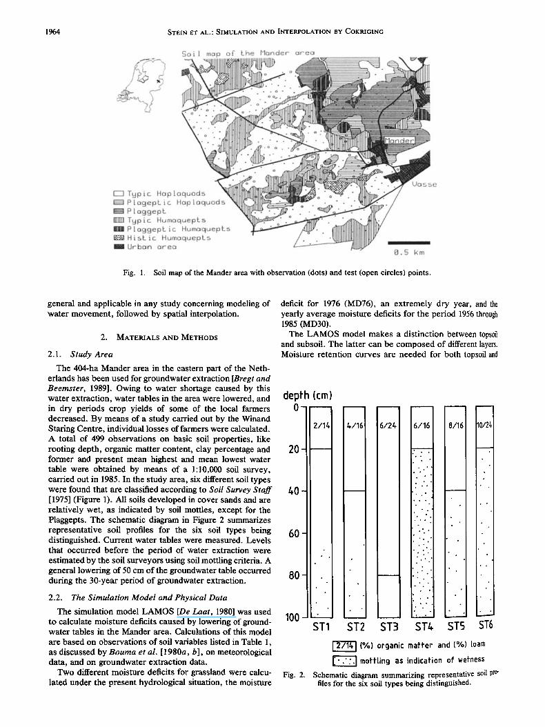
Fig. 1. Soil map of the Mander area with observation (dots) and test (open circles) pointsß

general and applicable in any study concerning modeling of water movement, followed by spatial interpolation.

2. MATERIALS AND METHODS

2.1. Study Area

The 404-ha Mander area in the eastern part of the Neth- erlands has been used for groundwater extraction [Bregt and Beeroster, 1989]. Owing to water shortage caused by this water extraction, water tables in the area were lowered, and in dry periods crop yields of some of the local farmers decreased. By means of a study carried out by the Winand Staring Centre, individual losses of farmers were calculated. A total of 499 observations on basic soil properties, like rooting depth, organic matter content, clay percentage and former and present mean highest and mean lowest water table were obtained by means of a 1:10,000 soil survey, carried out in 1985. In the study area, six different soil types were found that are classified according to Soil Survey Staff [1975] (Figure 1). All soils developed in cover sands and are relatively wet, as indicated by soil mottles, except for the Plaggepts. The schematic diagram in Figure 2 summarizes representative soil profiles for the six soil types being distinguished. Current water tables were measured. Levels that occurred before the period of water extraction were estimated by the soil surveyors using soil mottling criteria. A general lowering of 50 cm of the groundwater table occurred during the 30-year period of groundwater extraction.

2.2. The Simulation Model and Physical Data

The simulation model LAMOS [De Laat, 1980] was used to calculate moisture deficits caused by lowering of ground- water tables in the Mander area. Calculations of this model

are based on observations of soil variables listed in Table 1, as discussed by Bouma et al. [1980a, b], on meteorological data, and on groundwater extraction data.

Two different moisture deficits for grassland were calcu- lated under the present hydrological situation, the moisture

deficit for 1976 (MD76), an extremely dry year, and the yearly average moisture deficits for the period 1956 through 1985 (MD30).

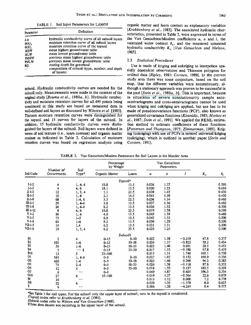
The LAMOS model makes a distinction between topsoil and subsoil. The latter can be composed of different layers. Moisture retention curves are needed for both topsoil and

depth {cm) O-

20-

60-

80-

100 - ST1 ST2 ST3 ST/, ST5 ST6

21/1• 1 (%) organic maft'er and (%) roam [-.':.]mottting as indication of wetness

Fig. 2. Schematic diagram summarizing representative soil pro- files for the six soil types being distinguished.

STEIN ET AL.' SIMULATION AND INTERPOLATION BY COKRIGING 1965

TABLE 1. Soil Input Parameters for LAMOS

Parameter Definition

k-h O(h)s O(h)t MHW MLW PMHW PMLW RD

hydraulic conductivity curve of all subsoil layers moisture retention curve of all subsoil layers moisture retention curve of the topsoil mean highest groundwater table mean lowest groundwater table previous mean highest groundwater table previous mean lowest groundwater table rooting depth for grassland composition of subsoil (type, number, and depth

of layers)

subsoil. Hydraulic conductivity curves are needed for the subsoil only. Measurements were made in the context of the original study [Bouma et al., 1980a, b]. Hydraulic conduc- tivity and moisture retention curves for all 499 points being considered in this study are based on measured data in well-defined soil layers as discussed by W6sten et al. [1985]. Thirteen moisture retention curves were distinguished for the topsoil and 15 curves for layers of the subsoil. In addition, 15 hydraulic conductivity curves were distin- guished for layers of the subsoil. Soil layers were defined in terms of soil texture (i.e., loam content) and organic matter content as indicated in Table 2. Calculation of moisture

retention curves was based on regression analysis using

organic matter and loam content as explanatory variables [Krabbenborg et al., 1983]. The associated hydraulic char- acteristics, presented in Table 2, were expressed in terms of the Van Genuchten/Mualem coefficients a, n and l, the saturated water content Os, and the measured saturated hydraulic conductivity K s [Van Genuchten and Nielsen, 1985].

2.3. Statistical Procedures

Use is made of kriging and cokriging to interpolate spa- tially dependent observations and Thiessen polygons for ordinal data [Ripley, 1981; Cotsten, 1989]. In the current study area there was some conjecture, based on the soil map, that the different variables were nonstationary, al- though a stationary approach was proven to be successful in the past [Stein et al., 1988a, b]. This is important, because in situations of severe nonstationarity sample auto- semivariograms and cross-semivariograms cannot be used when kriging and cokriging are applied, but use has to be made of pseudocovariance functions (PCF), also known as generalized covariance functions [Kitanidis, 1983 ; Morkoc et al., 1987; Stein et al., 1991]. We applied the REML estima- tion method to estimate coefficients of these functions

[Patterson and Thompson, 1975; Zimmerman, 1989]. Krig- ing (cokriging) with use of PCFs is termed universal kriging (cokriging), which is outlined in another paper [Stein and Cotsten, 1991].

TABLE 2. Van Genuchten/Mualem Parameters for Soil Layers in the Mander Area

Percentage Van Genuchten by Weight Parameters

Number of Soil

Soil Code Occurrences Type* Organic Matter Loam a n l Ks Os

Topsoil? I-1-2 4 1, 4, 6 10.8 13.5 I-I-5 4 4, 6 18.1 13.5

II-1-3 12 1, 3, 4 1.1 22.5 II-l-5 16 1, 4 2.1 14.5 II-1-9 68 1-4, 6 3.5 22.5

III-!-5 59 1, 4-6 3.8 13.5 !II-1-8 26 1, 4-6 6.2 13.5 III-l-12 8 4, 6 10.8 23.5 ¾-1-2 36 1, 4 4.0 13.5 V-l-5 73 1-5 6.0 13.5 V-l-8 61 1-6 9.5 13.5

¾II-1-5 14 !,4 6.2 13.5 VII-l-6 18 1, 3, 4 6.2 23.5

Subsoils B1 2 4 0-15 0-10 B2 105 1-6 0-15 10-18 B3 50 1-6 0-15 18-33 B4 1 '"õ 0-15 33-50 B16 13 5 23-100 O1 163 1, 4-6 0-3 0-10 02 420 1-6 0-3 10-18 03 75 2-4 0-3 18-33 04 12 4 0-3 33-50 05 6 --- 0-3 016 27 6 35-100 M 16 "' H8 22 6 $ 6 '--

0.026 1.27 0.590 0.020 1.25 0.610 0.028 1.45 0.420 0.041 1.39 0.430 0.036 1.34 0.460 0.027 1.36 0.460 0.026 1.32 0.500 0.019 1.28 0.590 0.045 1.39 0.480 0.042 1.33 0.500 0.030 1.29 0.530 0.021 1.31 0.500 0.025 1.25 0.500

0.022 1.58 -0.319 47.8 0.375 0.026 1.37 -0.825 59.3 0.434 0.022 1.40 0.001 28.5 0.453 0.017 1.52 -0.180 67.8 0.419 0.015 1.31 1.740 105.1 0.738 0.027 1.82 0.153 169.9 0.356 0.023 1.60 0.260 94.2 0.385 0.024 1.58 -0.118 87.8 0.352 0.018 1.53 0.137 185.5 0.359 0.049 1.87 0.605 396.3 0.334 0.019 1.27 -0.364 22.6 0.879 0.013 1.12 0.000 7.2 0.778 0.020 1.33 - 1.578 8.0 0.625 0.006 1.28 -4.241 0.4 0.375

*See Table 3 for soil types. For the subsoil only the upper layer of subsoil, next to the topsoil is considered. •Topsoil codes refer to Krabbenborg et al. [1983]. $Subsoil codes refer to W6sten and Van Genuchten [1988]. õThree dots denote not occurring in the upper layer of the subsoil.

1966 STEIN ET AL.: SIMULATION AND INTERPOLATION BY COKRiGING

In this study, commonly used polynomial trends of degree 1 and 2 are used to model the nonstationarity of the variables as compared to the stationary situation of a trend of degree 0 [Matheron, 1971]. One way to deal with this type of nonstationarity is to use increments of the observations instead of the observations themselves. The increments are

assumed to be stationary. For such increments the spatial structure is modeled by means of PCFs. In the main part of this paper we will investigate the use ofbivariate increments, and in the appendix we will discuss p-variate increments.

Several steps are necessary to deal with bivariate nonsta- tionary data. The first step is to form bivariate increments of the observations. The second step concerns the choice for a model to describe their spatial structure and the estimation of its parameters.

To obtain bivariate increments, consider n• observations of the variable Y• and n 2 observations of the variable Y2, which are summarized in a vector Y, of length n = n • + n2. The degree of the trend of the ith variable is denoted by vi. The monomials of a degree up to the degree of the trend of the coordinates of the observation locations of Yi are con- tained in the matrix X ii. On Y the transformation

= = =CY Z Z2 C2Y2 is applied, in which

of size N = N• + N2 by n, is such that both Zi and Z2 are vectors of univariate increments, that is, C iXii = 0 for i = 1, 2. For example, a matrix consisting of any Ni rows of C i '- (I- Xii(X?iXii)-lxii), one of the possibilities to subtract a polynomial trend from the observations, is a valid choice. For this particular choice, the PCFs describe the spatial structure of the corresponding residuals. In principle, the values of N•, i = 1, 2, need not be the same for the two variables. They are chosen such that a polynomial trend of degree v i is filtered.

The .second step concerns the estimation of the parameters of the PCFs. For bivariate increments the PCF is the sum of

the functions #•(r), #22(r) and O•2(r), each isotropic and linearly dependent on a vector •, of parameters:

gij(r) = Tij,oS(r) + Tij,•r + 'Yij,2 r3 + yij,3 r5 (1)

i,j=l, 2

where r is the distance between observation points, •5(r) = 1 if r = 0 and $(r) = 0 if r • 0. Here, g• (r) describes the spatial dependence of the predictand and g22(r) of the covariable, and •712(r) describes the spatial interaction be- tween predictand and covariable. As is well known [Delfther, 1976], the number of terms included in (1) depends on the degrees 1• i of the polynomial trends, that is, Vii, 2 r3 can be included only if v i exceeds 0, and Tii,3 r5 only if v i exceeds 1, whereas for i • j, Yij,2 r3 can be included only if vij, the minimum of b' i and vj, exceeds 0, and Tij,3 r5 only if vij exceeds 1, owing to the requirement of positive definite- ness [Stein et al., 1991].

The variance of increments of the observations, Q = Var (z) = E[zZ'ly], has a structure similar to (1), that is,

vl + 2 v2 + 2 v• + 2

k=l k=l k=l

(2)

where the matrices Q•j,•, = C G•j,kC' are of the size N x N. Elements of the matrix G ij,k are obtained from each of the constituent parts of (1) following the procedures in the appendix.

We assume that the N-dimensional Gaussian field f01. lowed by the N increments of the n observations is nonde. generate. Restrictions are imposed by the use of increments of the observations instead of the observations themselves. Estimation of the Yij,• is provided by minimizing the nega. tive log-likelihood function. This estimation procedure is commonly called the restricted maximum likelihood (REML) method [Patterson and Thompson, 1975]. In order to judge different degrees of trend, Akaikes' information criterion is used [Vecchia, 1988].

For estimating the coefficients, the total data set was too large to be handled efficiently. We therefore selected nine random sets, each of 25 elements. On each of these sets the coefficients of (2) were estimated. Nonpermissible coeffi- cients were assigned the value 0 [Delftnet, 1976]. The final coefficients are obtained by averaging the coefficients ob- tained for each of the nine sets. Whenever universal kriging was applied, a neighborhood of 18 observations was used. For universal cokriging the neighborhood was extended with 19 observations for the covariable.

Results from all procedures are compared by means of a test set of 100 locations which are randomly selected in advance from the complete set of the 499 borings. For the 100 test locations, the mean squared error (MSE), defined as the squared difference of predicted and observed values, is calculated:

100

1 • (MDc/- MDpi)2 (3) MSE = 100 i=1

where MDci is the calculated moisture deficit on the basis of measured profile characteristics in the ith test point, and MDpi is the predicted moisture deficit in the ith test point. Besides, to compare the kriging and the cokriging results, the mean variance of the prediction error (MVP) is calcu- lated as well for these points.

To investigate whether predicted values differ significantly in the mean from the original data, an adapted t test is used, in which the spatial structure of both the directly calculated data and predicted data is included [Stein et al., 1988a].

To distinguish among different procedures, Pitman's test of dispersion was applied [Pitman, 1939]. This test is appro- priate for comparing two dependent estimates s • and s• of the same population variance o -2 , assuming normality. Every MSE value is such an estimate, and every pair of MSE values is compared in this way. One calculates Cov [(X• ø X2), (X• + X2)], where X• is a prediction error of one procedure, that is, X•i = MDci - MD•,i, and X2 is a prediction error of another procedure. Under the assumption that X•i and X•i, as well as X2i and X2j, are independent f0r i % j, this results in a test stochastic, which follows at distribution.

Finally, biplots are constructed [Gabriel, 1971]. Bip10ts

STEIN ET AL.: SIMULATION AND INTERPOLATION BY COKRIGING 1967

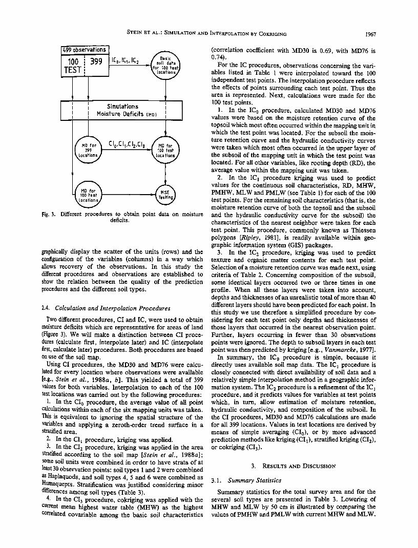
'"'Ob'servafions O0 i'" 399 EST:

l[ o, IC 1 , IE 2

' • Simutafions I Moisfure Befitifs I H•) I

C Io,E I•,œ1z,œ15

Fig. 3. Different procedures to obtain point data on moisture deficits.

graphically display the scatter of the units (rows) and the configuration of the variables (columns) in a way which allows recovery of the observations. In this study the different procedures and observations are established to show the relation between the quality of the prediction procedures and the different soil types.

2.4. Calculation and Interpolation Procedures

Two different procedures, CI and IC, were used to obtain moisture deficits which are representative for areas of land (Figure 3). We will make a distinction between C! proce- dures (calculate first, interpolate later) and IC (interpolate first, calculate later) procedures. Both procedures are based on use of the soil map.

Using CI procedures, the MD30 and MD76 were calcu- lated for every location where observations were available [e.g., Stein et al., 1988a, b]. This yielded a total of 399 values for both variables. Interpolation to each of the 100 test locations was carried out by the following procedures:

1. In the Ci 0 procedure, the average value of all point calculations within each of the six mapping units was taken. This is equivalent to ignoring the spatial structure of the variables and applying a zeroth-order trend surface in a stratified area.

2. in the CIt procedure, kriging was applied. 3. In the CI 2 procedure, kriging was applied in the area

stratified according to the soil map [Stein et ah, 1988a]; some soil units were combined in order to have strata of at

least 30 observation points: soil types 1 and 2 were combined as Hap!aquods, and soil types 4, 5 and 6 were combined as Humaquepts. Stratification was justified considering minor differences among soil types (Table 3). 4. In the CI 3 procedure, cokriging was applied with the

current mean highest water table (MHW) as the highest correlated covariable among the basic soil characteristics

(correlation coefficient with MD30 is 0.69, with MD76 is 0.74).

For the IC procedures, observations concerning the vari- ables listed in Table 1 were interpolated toward the I00 independent test points. The interpolation procedure reflects the effects of points surrounding each test point. Thus the area is represented. Next, calculations were made for the 100 test points.

1. In the IC0 procedure, calculated MD30 and MD76 values were based on the moisture retention curve of the topsoil which most often occurred within the mapping unit in which the test point was located. For the subsoil the mois- ture retention curve and the hydraulic conductivity curves were taken which most often occurred in the upper layer of the subsoil of the mapping unit in which the test point was located. For all other variables, like rooting depth (RD), the average value within the mapping unit was taken.

2. In the IC] procedure kriging was used to predict values for the continuous soil characteristics, RD, MHW, PMHW, MLW and PMLW (see Table 1) for each of the 100 test points. For the remaining soil characteristics (that is, the moisture retention curve of both the topsoil and the subsoil and the hydraulic conductivity curve for the subsoil) the characteristics of the nearest neighbor were taken for each test point. This procedure, commonly known as Thiessen polygons [RipIey, 1981], is readily available within geo- graphic information system (GIS) packages.

3. In the IC2 procedure, kriging was used to predict texture and organic matter contents for each test point. Selection of a moisture retention curve was made next, using criteria of Table 2. Concerning composition of the subsoil, some identical layers occurred two or three times in one profile. When all these layers were taken into account, depths and thicknesses of an unrealistic total of more than 40 different layers should have been predicted for each point. In this study we use therefore a simplified procedure by con- sidering for each test point only depths and thicknesses of those layers that occurred in the nearest observation point. Further, layers occurring in fewer than 30 observations points were ignored. The depth to subsoil layers in each test point was then predicted by kriging [e.g., Vanmarcke, 1977].

In summary, the IC0 procedure is simple, because it directly uses available soil map data. The IC] procedure is closely connected with direct availability of soil data and a relatively simple interpolation method in a geographic infor- mation system. The IC2 procedure is a refinement of the IC1 procedure, and it predicts values for variables at test points which, in turn, allow estimation of moisture retention, hydraulic conductivity, and composition of the subsoil. In the CI procedures, MD30 and MD76 calculations are made for all 399 locations. Values in test locations are derived by means of simple averaging (CI0), or by more advanced prediction methods like kriging (CId), stratified kriging (CI2), or cokriging (CI3).

3. RESULTS AND DISCUSSION

3.1. Summary Statistics

Summary statistics for the total survey area and for the several soil types are presented in Table 3. Lowering of MHW and MLW by 50 cm is illustrated by comparing the values of PMHW and PMLW with current MHW and MLW.

1968 STEIN ET AL.: SIMULATION AND INTERPOLATION BY COKRIGING

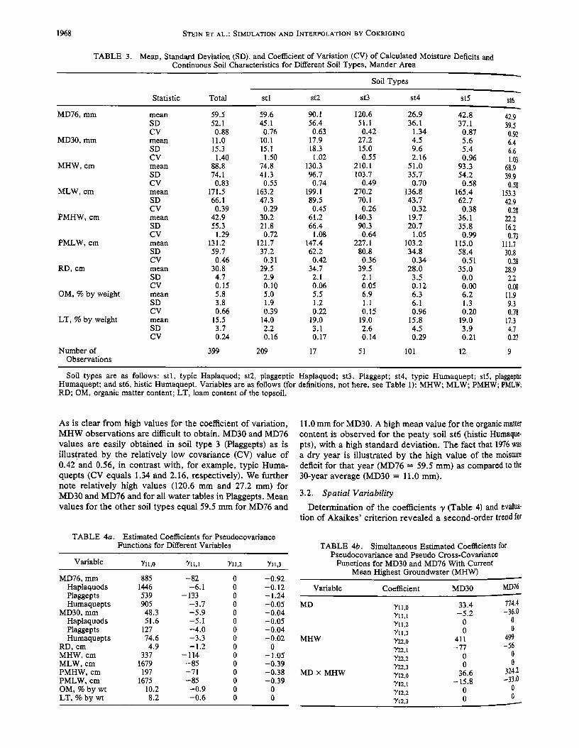
TABLE 3. Mean, Standard Deviation (SD), and Coefficient of Variation (CV) of Calculated Moisture Deficits and Continuous Soil Characteristics for Different Soil Types, Mander Area

Soil Types

Statistic Total st 1 st2 st3 st4 st5 st6

MD76, mm mean 59.5 59.6 90.1 120.6 26.9 42.8 42.9 SD 52.1 45.1 56.4 51.1 36.1 37.1 39.5 CV 0.88 0.76 0.63 0.42 1.34 0.87 0.92

MD30, mm mean 11.0 I0.1 17.9 27.2 4.5 5.6 6.4 SD 15.3 15.1 18.3 15.0 9.6 5.4 6.6 CV 1.40 1.50 1.02 0.55 2.16 0.96 1.03

MHW, cm mean 88.8 74.8 130.3 210.1 51.0 93.3 68.9 SD 74.1 41.3 96.7 103.7 35.7 54.2 39.9 CV 0.83 0.55 0.74 0.49 0.70 0.58 0.58

MLW, cm mean 171.5 163.2 199.1 270.2 136.8 165.4 153.3 SD 66.1 47.3 89.5 70.1 43.7 62.7 42.9 CV 0.39 0.29 0.45 0.26 0.32 0.38 0.28

PMHW, cm mean 42.9 30.2 61.2 140.3 19.7 36.1 22.2 SD 55.3 21.8 66.4 90.3 20.7 35.8 16.2 CV 1.29 0.72 1.08 0.64 1.05 0.99 0.73

PMLW, cm mean 131.2 121.7 147.4 227.1 103.2 115.0 111.7 SD 59.7 37.2 62.2 80.8 34.8 58.4 30.8 CV 0.46 0.31 0.42 0.36 0.34 0.51 0.28

RD, cm mean 30.8 29.5 34.7 39.5 28.0 35.0 28.9 SD 4.7 2.9 2.1 2.1 3.5 0.0 2.2 CV 0.15 0.10 0.06 0.05 0.12 0.00 0.08

OM, % by weight mean 5.8 5.0 5.5 6.9 6.3 6.2 1!.9 SD 3.8 1.9 1.2 1.1 6.1 1.3 9.3 CV 0.66 0.39 0.22 0.15 0.96 0.20 0.78

LT, % by weight mean 15.5 14.0 19.0 19.0 15.8 19.0 17.3 SD 3.7 2.2 3.1 2.6 4.5 3.9 4.7 CV 0.24 0.16 0.17 0.14 0.29 0.21 0.27

Number of 399 209 17 51 101 12 9 Observations

Soil types are as follows: stl, typic Haplaquod; st2, plaggeptic Haplaquod; st3, Plaggept; st4, typic Humaquept; st5, plaggeptic Humaquept; and st6, histic Humaquept. Variables are as follows (for definitions, not here, see Table 1): MHW; MLW; PMHW; PMLW: RD; OM, organic matter content; LT, loam content of the topsoil.

As is clear from high values for the coefficient of variation, MHW observations are difficult to obtain. MD30 and MD76

values are easily obtained in soil type 3 (Plaggepts) as is illustrated by the relatively low covariance (CV) value of 0.42 and 0.56, in contrast with, for example, typic Huma- quepts (CV equals 1.34 and 2.16, respectively). We further note relatively high values (120.6 mm and 27.2 mm) for MD30 and MD76 and for all water tables in Plaggepts. Mean values for the other soil types equal 59.5 mm for MD76 and

TABLE 4a. Estimated Coefficients for Pseudocovariance Functions for Different Variables

Variable 'Y11,0 T11,1 T11,2 T11,3

MD76, mm 885 -82 0 -0.92 Haplaquods 1446 -6.1 0 - 0.12 Plaggepts 539 - 133 0 - 1.24 Humaquepts 905 -3.7 0 -0.05

MD30, mm 48.3 -5.9 0 -0.04 Haplaquods 51.6 -5. I 0 -0.05 Plaggepts 127 -4.0 0 -0.04 Humaquepts 74.6 -3.3 0 -0.02

RD, cm 4.9 - 1.2 0 0 MHW, cm 337 - 114 0 - 1.05 MLW, cm 1679 -85 0 -0.39 PMHW, cm 197 -71 0 -0.38 PMLW, cm 1675 -85 0 -0.39 OM, % by wt 10.2 -0.9 0 0 LT, % by wt 8.2 -0.6 0 0

11.0 mm for MD30. A high mean value for the organic matter content is observed for the peaty soil st6 (histic Humaque- pts), with a high standard deviation. The fact that 1976 was a dry year is illustrated by the high value of the moisture deficit for that year (MD76 = 59.5 mm) as compared to the 30-year average (MD30 - 11.0 mm).

3.2. Spatial Variability

Determination of the coefficients ? (Table 4) and evalua- tion of Akaikes' criterion revealed a second-order trend for

TABLE 4b. Simultaneous Estimated Coefficients for Pseudocovariance and Pseudo Cross-Covariance

Functions for MD30 and MD76 With Current

Mean Highest Groundwater (MHW)

Variable Coefficient MD30

MD Yll,0 33.4 Yll,1 -5.2 Tll,2 0 Tll,3 0

MHW Y22,0 411 T22,1 --77 T22,2 0 T22,3 0

MD x MHW Yl2,0 36.6 Yl2,1 --15.8 T12,2 0 T12,3 0

MD76

774.4 -36.0

0

0

499 -56

0 0

324.2 -33.0

0

STEIN ET AL.' SIMULATION AND INTERPOLATION BY COKRIGING 1969

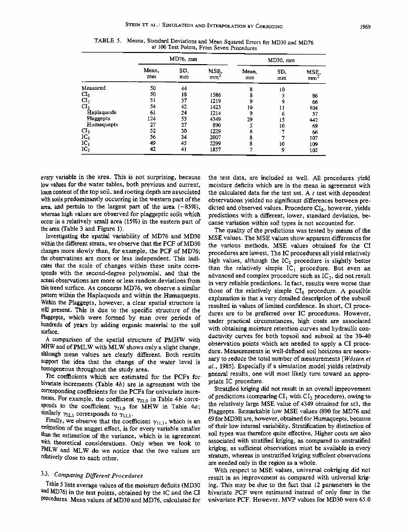
TABLE 5. Means, Standard Deviations and Mean Squared Errors for MD30 and MD76 at 100 Test Points, From Seven Procedures

MD76, mm MD30, mm

Mean, SD, MSE, Mean, SD, MSE, mm mm mm 2 mm mm mm 2

Measured

CI0 CI1 CI2

Haplaquods Plaggepts Humaquepts

CI3 IC0 IC1 IC2

50 44 8 10 50 18 1586 8 3 86 51 37 1219 9 9 66 54 42 1423 10 11 104 61 24 1214 9 6 57

124 53 4349 29 15 442 27 27 890 5 10 69 52 30 1229 8 7 66 56 34 2007 8 7 107 49 45 2299 8 10 109 42 41 1857 7 9 102

every variable in the area. This is not surprising, because low values for the water tables, both previous and current, loam content of the top soil, and rooting depth are associated with soils predominantly occurring in the western part of the area, and pertain to the largest part of the area (--•85%), whereas high values are observed for plaggeptic soils which occur in a relatively small area (15%) in the eastern part of the area (Table 3 and Figure 1).

Investigating the spatial variability of MD76 and MD30 within the different strata, we observe that the PCF of MD30 changes more slowly than, for example, the PCF of MD76; the observations are more or less independent. This indi- cates that the scale of changes within these units corre- sponds with the second-degree polynomial, and that the actual observations are more or less random deviations from

this trend surface. As concerns MD76, we observe a similar pattern within the Haplaquods and within the Humaquepts. Within the Plaggepts, however, a clear spatial structure is still present. This is due to the specific structure of the Plaggepts, which were formed by man over periods of hundreds of years by adding organic material to the soil surface.

A comparison of the spatial structure of PMHW with MHW and of PMLW with MLW shows only a slight change, although mean values are clearly different. Both results support the idea that the change of the water level is homogeneous throughout the study area.

The coefficients which are estimated for the PCFs for bivariate increments (Table 4b) are in agreement with the corresponding coefficients for the PCFs for univariate incre- ments. For example, the coefficient 3'22,0 in Table 4b corre- sponds to the coefficient •/l•,0 for MHW in Table 4a; similarly Y22,1 corresponds to

Finally, we observe that the coefficient •/•.•, which is an estimation of the nugget effect, is for every variable smaller than the estimation of the variance, which is in agreement with theoretical considerations. Only when we look to PMLW and MLW do we notice that the two values are relatively close to each other.

3.3. Comparing Different Procedures Table 5 lists average values of the moisture deficits (MD30

and MD76) in the test points, obtained by the IC and the CI procedures. Mean values of MD30 and MD76, calculated for

the test data, are included as well. All procedures yield moisture deficits which are in the mean in agreement with the calculated data for the test set. A t test with dependent observations yielded no significant differences between pre- dicted and observed values. Procedure CI0, however, yields predictions with a different, lower, standard deviation, be- cause variation within soil types is not accounted for.

The quality of the predictions was tested by means of the MSE values. The MSE values show apparent differences for the various methods. MSE values obtained for the CI

procedures are lowest. The IC procedures all yield relatively high values, although the IC2 procedure is slightly better than the relatively simple IC• procedure. But even an advanced and complex procedure such as IC 2, did not result in very reliable predictions. In fact, results were worse than those of the relatively simple CI0 procedure. A possible explanation is that a very detailed description of the subsoil resulted in values of limited confidence. In short, CI proce- dures are to be preferred over IC procedures. However, under practical circumstances, high costs are associated with obtaining moisture retention curves and hydraulic con- ductivity curves for both topsoil and subsoil at the 30-40 observation points which are needed to apply a CI proce- dure. Measurements in well-defined soil horizons are neces-

sary to reduce the total number of measurements [WOsten et a!., 1985]. Especially if a simulation model yields relatively general results, one will most likely turn toward an appro- priate IC procedure.

Stratified kriging did not result in an overall improvement of predictions (comparing CI• with CI 2 procedure), owing to the relatively large MSE value of 4349 obtained for st3, the Plaggepts. Remarkable low MSE values (890 for MD76 and 69 for MD30) are, however, obtained for Humaquepts, because of their low internal variability. Stratification by distinction of soil types was therefore quite effective. Higher costs are also associated with stratified kriging, as compared to unstratified kriging, as sufficient observations must be available in every stratum, whereas in unstratified kriging sufficient observations are needed only in the region as a whole.

With respect to MSE values, universal cokriging did not result in an improvement as compared with universal krig- ing. This may be due to the fact that 12 parameters in the bivariate PCF were estimated instead of only four in the univariate PCF. However, MVP values for MD30 were 65.0

1970 STEIN ET AL.' SIMULATION AND INTERPOLATION BY COKR1GING

2 •

--1 -

--2

--3 -

--4

A C

c

c

B AA

A

B

A A

c c c c c c

A C A

A

c œ

A

c c

c

c c

ICO

c c c ^ ^ C2

A A

ClO

CI2

---4 --3 ---2 ..-1 0 1 2 3 4

FACTOR1

Fig. 4a

Fig. 4. Biplot for (a) MD30 and (b) MD76. Labels denote soil types: A, Haplaquods; B, Plaggepts' and C, Humaquepts. Larger characters denote the mean values.

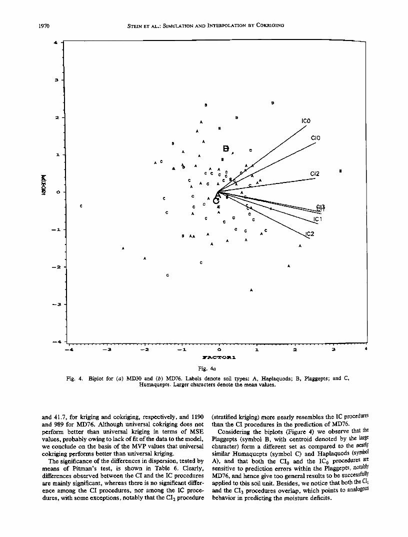
and 41.7, for kriging and cokriging, respectively, and 1190 and 989 for MD76. Although universal cokriging does not perform better than universal kriging in terms of MSE values, probably owing to lack of fit of the data to the model, we conclude on the basis of the MVP values that universal

cokriging p.erforms better than universal kriging. The significance of the differences in dispersion, tested by

means of Pitman's test, is shown in Table 6. Clearly, differences observed between the CI and the IC procedures are mainly significant, whereas there is no significant differ- ence among the CI procedures, nor among the IC proce- dures, with some exceptions, notably that the CI2 procedure

(stratified kriging) more nearly resembles the IC procedures than the CI procedures in the prediction of MD76.

Considering the biplots (Figure 4) we observe that the Plaggepts (symbol B, with centroid denoted by the large character) form a different set as compared to the nearly similar Humaquepts (symbol C) and Haplaquods (symbol A), and that both the CI0 and the !C0 procedures are sensitive to prediction errors within the Plaggepts, notably MD76, and hence give too general results to be successfully applied to this soil unit. Besidesl we notice that both the CI• and the CI3 procedures overlap, which points to analogous behavior in predicting the moisture deficits.

STEIN ET AL.' SIMULATION AND INTERPOLATION BY COKRIGING 1971

3

--2

-.3

---4

½ A

B B B

A A

c Aœ :•Cc AC C A C

C A

A A

A

Fig. 4b

ICO

cIo

B

CI2

^ IC2

C c C

A A A

-1 2 3 4

TABLE 6. Significance Shown by Pitman's Test of Differences in Dispersion of Mean Squared Error Values Between the Different Procedures

MD30 MD76

CI1 CI2 CI3 ICo IC1 IC2 CI• CI2 CI3 ICo IC] IC2 CIo CI] CI2 CI3 ICo IC 1

Levels of significance are denoted by asterisks: *, significant at 5% level; **, significant at 1% level; ***, significant at 0.1% level.

1972 STEIN ET AL.: SIMULATION AND INTERPOLATION BY COKRIGING

4. CONCLUSIONS

1. When values for moisture deficits are to be obtained

for areas of land, it appears from this study that the best way to proceed is first to simulate for every location where observations are available, and then to apply statistical interpolation techniques for the area, although higher costs for data collection may be prohibitive.

2. Stratification according to soil type is quite effective to improve the quality of predictions within the strata.

3. Universal cokriging performs better than universal kriging, as evidenced by lower prediction error variances for the test set.

APPENDIX: ESTIMATING THE PARAMETERS OF A

LINEAR PSEUDOCOVARIANCE FUNCTION

WITH THE REML ESTIM^TIOr4 METHOD

Let there be n observations on p variables, collected in the vector Y. The upper n• part contains the n l observations of the predictand, the following n 2 part the n 2 observations of the first covariable, etc., n = •;ni. The degree of polynomial trend which accounts for the nonstationarity of the ith variable is denoted by •'i. An increment is any linear combination •'Y of the observations for which (1) E[,k'Y] - 0; and (2) Var [X' Y] = ,• GA, where the matrix G is derived from pseudocovariance f•tnctions gu•,: RdxR d '--> R, which depend on a m vector 3' of parameters; G has to be such that X'G• -> 0 for all X'Y, with E[X'Y] = 0.

The collection of ,k values satisfying 1 and 2 is called the collection of permissible X values. It forms a finite- dimensional linear space, for which the elements of any basis of the space may be arranged as rows of the matrix C. Any linear combination of the elements of the vector Z = C Y is

an increment. Conversely, any increment of the observa- tions can be expressed as a linear combination of the elements of the vector Z = CY [Kitanidis, 1983; Barendregt, 1987]. For example, the matrix

1 0

c = ... = x(x'x)-x ') Cp

can be used, where X is a partitioned matrix with blocks Xij, with X U = 0 for i V: j and Xii contains k i multivariate monomials of the coordinates of the observation locations of

the ith variable up to v•. In this case, the last k i rows of Xii may be skipped, as the rank of Ci equals Ni, yielding a matrix C of size N = 5•N i by n. Incidentally, we notice that the value of N i is equal to ni- ki, where ki = 1 if •'i = 0, k i = 3 ff •'i = 1, and k i = 6 if •'i = 2 and hence that

p p p

S = X Si = X gli- X (l"i q- 1)(/2i q- 2)/2 (A2) i=1 i=1 i=1

Concerning the distribution we assume that the vector Z has a Gaussian distribution with zero mean and variance

matrix Q = CGC', linear in the vector y:

Q = T1Q1 + T2Q2 +" '+ TmQm (A3)

where Q i, '", Qm are known matrices and yl, .-., 3'm are unknown parameters. As is shown by standard methods,

the likelihood equations are Tr (Q-1QiQ-l(z. z' - Q))• 0 for i = 1, ..- , m, which is equivalent to the following system of linear equations:

Tr (Q-•Q•Q-1Z. z') = Tr (Q-IQ1Q-1Q1)T 1 +...

+ Tr (Q-1Q•Q-•Qm)? m ! (A4)

tr (Q-iQmQ-iZ ß Z')= Tr (Q-IQmQ-iQi)3'i +...

+ tr (Q-iQ,nQ-iQm)?• A procedure to solve these equations is, after a prior estimate of Q, to solve the 3' vectol'• and to calculate a new Q, which is equivalent to Newton's method [Kitanidis, 1983]. The calculation is repealed until convergence is achieved. This procedure, commonly known as the re- stricted maximum likelihood (REML) approach, maximizes the likelihood of the parameter 3' for the observed incre- ments. It is noted that the REML estimate does not depend on the choice of the basis of increments.

A key statistic to distinguish between various degrees 0t trends is Akaikes' information criterion. This is defined as

A = l(ZI3') + 2m (AS)

•here l(Z I y) is the log-likelihood function. The degree of the trend which minimizes (AS) is considered the appropriate degree of nonstationarity.

. Acknowledgments. This research was sponsored by the Nether- lands Integrated Soil Research Program. Helpful discussions with H. W6sten of the Winand Stating Centre and A. Otten from the Department of Statistics of the Wageningen Agricultural University are gratefully acknowledged.

REFERENCES

Barendregt, L. G., The estimation of generalized covariance whenit is a linear combination of two known generalized covariances, Water Resour. Res., 23, 583-590, 1987.

Bouma, J., Land qualities in space and time, in Land Qualities in Space and Time, edited by J. Bouma, and A. K. Bregt, pp. 2-13, Pudoc, Wageningen, Netherlands, 1989a.

Bouma, J., Using soil survey data for quantitative land evaluation, in Adv. in Soil $ci., 177-213, 1989b.

Bouma, J., P. J. M. De Laat, A. F. Van Hoist, and T. J. Van de Nes, Predicting the effects of changing water-table levels and associ- ated soil moisture regimes for soil survey interpretations, Soil $ci. Soc. Am. J., 44, 797-802, I980a.

Bouma, J., P. J. M. De Laat, R. H. C. M. Awater, H. C. Van Heesen, A. F. Van Holst, and T. J. Van de Nes, Use of s0il survey data in a model for simulating regional soil moisture regimes, Soil Sci. Soc. Am. J., 44, 808-814, 1980b.

Bregt, A. K., and J. G. R. Beemster, Accuracy in predicting moisture deficits and changes in yield from soil maps, Geoderma, 43, 301-310, 1989.

Corsten, L. C. A., Interpolation and optimal linear prediction, star. Neer., 43, 69-84, 1989.

Cressie, N., Kriging nonstationary data, JASA J. Am. Stat. Assoc., 81,625-634, 1986.

De Laat, P. J. M., Model for unsaturated flow above a shallow water table, applied to a regional subsurface problem, Agric. Res. Rep. 895, Pudoc, Wageningen, Netherlands, 1980.

D½lfiner, P., Linear estimation of nonstationary spatial phenomena, in Advanced Geostatistics in the Mining Industry, edited by M. Guarascio, M. David, and C. Huijbregts, pp. 49-68, D. Reidel, Hingham, Mass., 1976.

STEIN ET AL.: SIMULATION AND INTERPOLATION BY COKRIGING 1973

De Wit, C. T., and H. Van Keulen, Modelling production of field crops and its requirements, Geoderma, 40, 253-267, 1985.

Feddes, R. A., P. J. Kowalik, and H. Zaradny, Simulation of Field Water Use and Crop Yield, 109 pp., Pudoc, Wageningen, Neth- erlands, 1978.

Gabriel, K. R., The hiplot-graphic display of matrices with applica- tion to principal component analysis, Biometrika, 58, 453-467, 1971.

Kitanidis, P., Statistical estimation of polynomial generalized cova- dance functions and hydrologic applications, Water Resour. Res., 19, 909-921, 1983.

Krabbenborg, A. J., J. N. B. Poelman, and E. J. Van Zuilen, Standaardvochtkarakteristieken van Zandgronden en Veenkolo- niale Gronden, Vols. I and II, 330 pp., Stichting voor Bodemkar- tering, Wageningen, Netherlands, 1983.

Mardia, K. V., and R. J. Marshall, Maximum likelihood estimation of models for residual covariance in spatial regression, Bio- metrika, 71, 135-146, 1984.

Matheron, G., The theory of regionalized variables and its applica- tions, Cah. Cent. Morphol. Math., 5, 211 pp., 1971.

Morkoc, F., J. W. Biggar, D. R. Nielsen, and D. E. Myers, Kriging with generalized covariances, Soil Sci. Soc. Am. J., 51, 1126- 1!31, 1987.

Patterson, H. D., and R. Thompson, Maximum likelihood estima- tion of components of variance, in Proceedings of the 8th Inter- national Biometric Conference Constanta, edited by L. C. A. Corsten and T. Postelnicu, pp. 197-207, Editura Academiei Re- publicii Socialisti Romania, Bucharest, 1975.

Pitman, E.G., A note on normal correlation, Biometrika, 31, 9-!2, 1939.

Ripley, B. D., Spatial Statistics, 252 pp., John Wiley, New York, 1981.

S0il Survey Staff, Soil taxonomy, a basic system of soil classifica- tion for making and interpreting soil surveys, Agric. Hahrib. 436, Soil Conserv. Serv., U.S. Dep. of Agric., Washington, D.C., 1975.

Stein, A., and L. C. A. Corsten, Universal kriging and cokriging as a regression procedure, Biometrics, in press, 1991.

Stein, A., M. Hoogerwerf, and J. Bouma, Use of soil map delinea- tions to improve (co-)kriging of point data on moisture deficits, Geoderma, 43, 163-177, 1988a.

Stein, A., J. Bouma, W. Van Dooremolen, and A. K. Bregt,

Cokriging point data on moisture deficit, Soil Sci. Soc. Am. J., 52, 1418-1423, 1988b.

Stein, A., J. Bouma, M. A. Mulders, and M. H. W. Wererings, Using cockfiging in variability studies to predict physical land qualities of a level river terrace, Soil Technol., 2, 385-402, 1989.

Stein, A., A. C. Van Eijnsbergen, and L. G. Barendregt, Cokriging nonstationary data, Math. Geol., in press, 1991.

Van Genuchten, M. T., and D. R. Nielsen, On describing and predicting the hydraulic properties of unsaturated soils, Ann. Geophys., 3, 615-628, 1985.

Vanmarcke, E. H., Probabilistic modeling of soil profiles, J. Geo- tech. Eng. Div., Am. Soc. Civ. Eng., I03, 1227-1246, 1977.

Vauclin, M., S. R. Vieira, G. Vachaud, and D. R. Nielsen, The use of cokriging with limited field soil observations, Soil Sci. Soc. Am. J., 47, 175-184, 1983.

Vecchia, A. V., Estimation and model identification for continuous spatial processes, J. R. Stat. Soc. B, 50, 297-312, 1988.

W6sten, J. H. M., and M. T. Van Genuchten, Using texture and other soil properties to predict the unsaturated soil hydraulic functions, Soil Sci. Soc. Am. J., 52, 1762-1770, 1988.

W6sten, j. H. M., J. Bouma, and G. H. Stoffelsen, Use of soil survey data for regional soil water simulation models, Soil Sci. Soc. Am. J., 47, 175-184, 1985.

Yates, S. R., and A. W. Warrick, Estimating soil water content using cokriging, Soil Sci. Soc. Am. J., 51, 23-30, 1987.

Zimmerman, D. L., Computationally efficient restricted maximum likelihood estimation of generalized covariance functions, Math. Geol., 21,655-672, 1989.

J. Bouma, I. G. Staritsky, and A. Stein, Department of Soil Science and Geology, Agricultural University, P.O. Box 37, 6700 AA Wageningen, Netherlands.

A. K. Bregt, Winand Staring Centre for Integrated Land, Soil and Water Research, P.O. Box 125, 6700 AC Wageningen, Netherlands.

A. C. Van Eijnsbergen, Department of Mathematics, Agricultural University, Dreijenlaan 4, 6703 BC Wageningen, Netherlands.

(Received October 3, 1990; revised February 10, 1991;

accepted February 20, 1991.)