Regularization Paths for Generalized Linear Models via Coordinate Descent
Upload
khangminh22Category
view
0download
0
Journal of Machine Learning Research () Submitted 12/08; Published
Maximum Relative Margin and Data-Dependent Regularization
Pannagadatta K. Shivaswamy [email protected] .EDU
Tony Jebara [email protected] .EDU
Department of Computer ScienceColumbia UniversityNew York, NY 10027, USA
Editor: John Shawe-Taylor
AbstractLeading classification methods such as support vector machines (SVMs) and their counterparts
achieve strong generalization performance by maximizing the margin of separation between dataclasses. While the maximum margin approach has achieved promising performance, this articleidentifies its sensitivity to affine transformations of the data and to directions with large data spread.Maximum margin solutions may be misled by the spread of data and preferentially separate classesalong large spread directions. This article corrects theseweaknesses by measuring margin not inthe absolute sense but rather only relative to the spread of data in any projection direction. Maxi-mum relative margin corresponds to a data-dependent regularization on the classification functionwhile maximum absolute margin corresponds to anℓ2 norm constraint on the classification func-tion. Interestingly, the proposed improvements only require simple extensions to existing maximummargin formulations and preserve the computational efficiency of SVMs. Through the maximiza-tion of relative margin, surprising performance gains are achieved on real-world problems suchas digit, text classification and on several other benchmarkdatasets. In addition, risk bounds arederived for the new formulation based on Rademacher averages.
Keywords: Support Vector Machines, Kernel Methods, Large Margin, Rademacher Complexity
1. Introduction
In classification problems, the aim is to learn a classifier that generalizes well on future data froma limited number of training examples. Support vector machines (SVMs) and maximum marginclassifiers (Vapnik, 1995; Scholkopf and Smola, 2002; Shawe-Taylor and Cristianini, 2004) havebeen a particularly successful approach both in theory and in practice. Given a labeled trainingset, these return a predictor that accurately labels previously unseen test examples. For simple bi-nary classification in Euclidean spaces, this predictor is afunction f : R
m → {±1} estimated fromobserved training data(xi,yi)
ni=1 consisting of inputsxi ∈ R
m and outputsyi ∈ {±1}. A linear func-tion1 f (x) := sign(w⊤x+b) wherew∈R
m,b∈R serves as the decision rule throughout this article.The parameters of the hyperplane(w,b) are estimated by maximizing the margin (e.g., the distancebetween the hyperplanes defined byw⊤x+b= 1 andw⊤x+b = −1) while minimizing a weightedupper bound on the misclassification rate on training data (via so-called slack variables). In practice,the margin is maximized by minimizing12w⊤w plus an upper bound on the misclassification rate.
1. In this article the dot productw⊤x is used with the understanding that it can be replaced with a generalized innerproduct or by using a kernel for generic objects.
c© Pannagadatta K. Shivaswamy and Tony Jebara.

SHIVASWAMY AND JEBARA
While maximum margin classification works well in practice,its solution can easily be perturbedby an (invertible) affine or scaling transformation of the input space. For instance, by transformingall training and testing inputs by an invertible linear transformation, the SVM solution and its re-sulting classification performance can be significantly varied. This is worrisome since an adversarycould directly exploit this shortcoming and transform the data to drive performance down; a syn-thetic example showing this effect will be presented in Section 5. Moreover, this phenomenon isnot limited to an explicit adversarial setting; it can naturally occur in many real world classificationproblems, especially in high dimensions. This article willexplore such shortcomings in maximummargin solutions (or equivalently, SVMs in the context of this article) which exclusively measuremargin by the points near the classification boundary regardless of how spread the remaining data isaway from the separating hyperplane. An alternative approach will be followed based on controllingthe spread while maximizing the margin. This helps overcomethis bias and produces a formulationthat is affine invariant. The key is to recover a large margin solution while normalizing the marginby the spread of the data. Thus, margin is measured in arelative sense rather than in the absolutesense. In addition, theoretical results using Rademacher averages support this intuition. The re-sulting classifier will be referred to as the relative marginmachine (RMM) and was first introducedby Shivaswamy and Jebara (2009a) with this longer article serving to provide more details, morethorough empirical evaluation and more theoretical support.
Traditionally, controlling spread has been an important theme in classification problems. For in-stance, classical linear discriminant analysis (LDA) (Duda et al., 2000) finds projections of the dataso that the inter-class separation is large while within-class scatter is small. However, the spread (orscatter in this context) is estimated by LDA using only simple first and the second order statistics ofthe data. While this is appropriate if class-conditional densities are Gaussian, second-order statis-tics are inappropriate for many real-world datasets and thus, the classification performance of LDAis typically weaker than that of SVMs. The estimation of spread should not make second-orderassumptions about the data and should be tied to the margin criterion (Vapnik, 1995). A similarline of reasoning has been proposed to perform feature selection. Weston et al. (2000) showed thatsecond order tests and filtering methods on features performpoorly compared to wrapper methodson SVMs which more reliably remove features that have low discriminative value. In this priorwork, a feature’s contribution to margin is compared to its effect on the radius of the data by com-puting bounding hyper-spheres rather than simple Gaussianstatistics. Unfortunately, there, onlyaxis-aligned feature selection was considered. Similarly, ellipsoidal kernel machines (Shivaswamyand Jebara, 2007) were proposed to normalize data in featurespace by estimating bounding hyper-ellipsoids while avoiding second-order assumptions. Similarly, the radius-margin bound has beenused as a criterion to tune the hyper-parameters of the SVM (Keerthi, 2002). Another criterion basedjointly on ideas from the SVM method as well as Linear Discriminant Analysis has been studiedby Zhang et al. (2005). This technique involves first solvingthe SVM and then solving an LDAproblem based on the support vectors that were obtained. While these previous methods showedperformance improvements, they relied on multiple-step locally optimal algorithms for interleavingspread information with margin estimation.
To overcome the limitations of local non-convex optimization schemes, the formulations derivedhere will remain convex, will be efficiently solvable and will admit helpful generalization bounds.A similar method to the RMM was described by Haffner (2001), yet that approach started from adifferent overall motivation. In contrast, this article starts with a novel intuition, produces a novelalgorithm and provides novel empirical and theoretical support. Another interesting contact point
2

MAXIMUM RELATIVE MARGIN AND DATA -DEPENDENTREGULARIZATION
is the second order perceptron framework (Cesa-Bianchi et al., 2005) which parallels some of theintuitions underlying the RMM. In an on-line setting, the second order perceptron maintains botha decision rule and a covariance matrix to whiten the data. The mistake bounds it inherits wereshown to be better than those of the classical perceptron algorithm. Alternatively, one may considerdistributions over classifier solutions which provide a different estimate than the maximum marginsetting and have also shown empirical improvements over SVMs (Jaakkola et al., 1999; Herbrichet al., 2001). In recent papers, Dredze et al. (2008); Crammer et al. (2009a) consider a distributionon the perceptron hyperplane. These distribution assumptions permit update rules that resemblewhitening of the data, thus alleviating adversarial affine transformations and producing changes tothe basic maximum margin formulation that are similar in spirit to those the RMM provides. Inaddition, recently, a new batch algorithm called the Gaussian margin machine (GMM) (Crammeret al., 2009b) has been proposed. The GMM maintains a Gaussian distribution over weight vectorsfor binary classification and seeks the least informative distribution that correctly classifies trainingdata. While the GMM is well motivated from a PAC-Bayesian perspective, the optimization problemitself is expensive involving a log-determinant optimization.
Another alternative route for improving SVM performance includes the use of additional exam-ples. For instance, unlabeled or test examples may be available in semi-supervised or transductiveformulations of the SVM (Joachims, 1999; Belkin et al., 2005). Alternatively, additional data thatdoes not belong to any of the classification classes of interest may be available as in the so-calledUniversum approach (Weston et al., 2006; Sinz et al., 2008).In principle, these methods also changethe way margin is measured and the way regularization is applied to the learning problem. Whileadditional data can be helpful in overcoming limitations for many classifiers, this article will beinterested in only the simple binary classification setting. The argument is that, without any ad-ditional assumptions beyond the simple classification problem, maximizing margin in the absolutesense may be suboptimal and that maximizing relative marginis a promising alternative.
Further, large margin methods have been successfully applied to a variety of tasks such asparsing (Collins and Roark, 2004; Taskar et al., 2004), matrix factorization (Srebro et al., 2005),structured prediction (Tsochantaridis et al., 2005) etc.;in fact, the RMM approach could be read-ily adapted to such problems. For instance, RMM has been successfully extended to structuredprediction problems (Shivaswamy and Jebara, 2009b).
The organization of this article is as follows. Motivation from various perspectives are given inSection 2. The relative margin machine formulation is detailed in Section 3 and several variants andimplementations are proposed. Generalization bounds for the various function classes are studiedin Section 4. Experimental results are provided in Section 5. Finally, conclusions are presented inSection 6. Some proofs and otherwise standard results are provided in the Appendix.
Notation Throughout this article, boldface letters indicate vectors/matrices. For two vectorsu ∈R
m andv ∈ Rm, u ≤ v indicates thatui ≤ vi for all i from 1 tom. 1, 0 andI denote the vectors of
all ones, all zeros and the identity matrix respectively;0 also denotes a matrix of all zeros in somecontexts. The dimensionality of vectors and matrices should be clear from the context.
2. Motivation
This section provides three different (an intuitive, a probabilistic and an affine transformation based)motivations for maximizing the margin relative to the data spread.
3

SHIVASWAMY AND JEBARA
2.1 Intuitive motivation with a two dimensional example
Consider the simple two dimensional dataset in Figure 1 where the goal is to separate the two classesof points: triangles and squares. The figure depicts three scaled versions of the two dimensionalproblem to illustrate potential problems with the large margin solution.
In the topmost plot in the left column of Figure 1, two possible linear decision boundariesseparating the classes are shown. The red (or dark shade) solution is the SVM estimate whilethe green (or light shade) solution is the proposed maximum relative margin alternative. Clearly,the SVM solution achieves the largest margin possible whileseparating both classes, yet is thisnecessarily the best solution?
Next, consider the same set of points after a scaling transformation in the second and the thirdrow of Figure 1. Note that all these three problems correspond to the same discrimination problemup to a scaling factor. With progressive scaling, the SVM increasingly deviates from the maximumrelative margin solution (green), clearly indicating thatthe SVM decision boundary is sensitive toaffine transformations of the data. Essentially, the SVM produces a family of different solutions as aresult of the scaling. This sensitivity to scaling and affinetransformations is worrisome. If the SVMsolution and its generalization accuracy vary with scaling, an adversary may exploit such scaling toensure that the SVM performs poorly. Meanwhile, an algorithm producing the maximum relativemargin (green) decision boundary could remain resilient toadversarial scaling.
In the previous example, a direction with a small spread in the data produced a good and affine-invariant discriminator which maximized relative margin.Unlike the maximum margin solution,this solution accounts for the spread of the data in various directions. This permits it to recover asolution which has a large margin relative to the spread in that direction. Such a solution wouldotherwise be overlooked by a maximum margin criterion. A small margin in a correspondinglysmaller spread of the data might be better than a large absolute margin with correspondingly largerdata spread. This particular weakness in large margin estimation has only received limited attentionin previous work.
It is helpful to consider the generative model for the above motivating example. Therein, eachclass was generated from a one dimensional line distribution with the two classes on two parallellines. In this case, the maximum relative margin (green) decision boundary should obtain zero testerror even if it is estimated from a finite number of examples.However, for finite training data,the SVM solution will make errors and will do so increasinglyas the data is scaled further. Whileit is possible to anticipate these problems and choose kernels or nonlinear mappings to correct forthem in advance, this is not necessarily practical. The right mapping or kernel is never provided inadvance in realistic settings. Instead, one has to estimatekernels and nonlinear mappings, a difficultendeavor which can often exacerbate the learning problem. Similarly, simple data preprocessing(affine whitening to make the dataset zero-mean and unit-covariance or scaling to place the datainto a zero-one box) can also fail, possibly because of estimation problems in recovering the correcttransformation (this will be shown in real-world experiments).
The above arguments show that large margin on its own is not enough; it is also necessary tocontrol the spread of the data after projection. Therefore,maximum margin should be traded-off orbalanced with the goal of simultaneously minimizing the spread of the projected data, for instance,by bounding the spread|w⊤x + b|. This will allow the linear classifier to recover large marginsolutions not in the absolute sense but ratherrelative to the spread of the data in that projectiondirection.
4

MAXIMUM RELATIVE MARGIN AND DATA -DEPENDENTREGULARIZATION
Figure 1: Left: As the data is scaled, the maximum margin SVM solution (red or dark shade) de-viates from the maximum relative margin solution (green or light shade). Three differentscaling scenarios are shown. Right: The projections of the examples (that isw⊤x+b) onthe real line for the SVM solution (red or dark shade) and the proposed classifier (green orlight shade) under each scaling scenario. These projections have been drawn on separatedaxes for clarity. The absolute margins for the maximum margin solution (red) are 1.24,1.51 and 2.08 from top to bottom. For the maximum relative margin solution (green)the absolute margin is merely 0.71. However, the relative margin (the ratio of absolutemargin to the spread of the projections) is 41%, 28%, and 21% for the maximum marginsolution (red) and 100% for the relative margin solution (green). The scale of all axes iskept locked to permit direct visual comparison.
5

SHIVASWAMY AND JEBARA
In the case of a kernel such as the RBF kernel, the points are first mapped to a space so thatall the input examples are unit vectors (i.e.,〈φ(x),φ(x)〉 = 1). Note that the intuitive motivationproposed here still applies in such cases. No matter how theyare mapped initially, a large marginsolution still projects these points to the real line where the margin of separation is maximized.However, the spread of the projection can still vary significantly among the different projectiondirections. Given the above motivation, it is important to achieve a large margin relative to the spreadof the projections even in such situations. Furthermore, experiments will support this intuition withdramatic improvements on many real problems and with a variety of kernels (including radial basisfunction and polynomial kernels).
2.2 Probabilistic motivation
In this subsection, an informal motivation is provided to illustrate why maximizing relative marginmay be helpful. Suppose(xi ,yi)
ni=1 are drawn independently and identically (iid) from a distribution
D. A classifierw∈Rm is sought which will produce low error on future unseen examples according
to the decision rule ˆy = sign(w⊤x). An alternative criterion is that the classifier should produce alarge value ofη according to the following expression:
Pr(x,y)∼D
[
yw⊤x ≥ 0]
≥ η,
wherew ∈ Rm is the classifier. One way to ensure the above constraint is byrequiring that the
following inequality hold:
ED [yw⊤x] ≥√
η1−η
√
VD [yw⊤x]. (1)
A proof of the above claim for a general distribution can be found in Shivaswamy et al. (2006). Infact, Gaussian margin machines (Crammer et al., 2009b) start with a similar motivation but assumea Gaussian distribution on the classifier.
According to (1), achieving a low probability of error requires the projections to have a largemean and a small variance. The mean and variance for the true distributionD may be unavailable,however, the empirical counterparts of these quantities are available and known to be concentrated.The above inequality is used as a loose motivation. Instead of precisely finding low variance andhigh mean projections, this paper implements this intuition by trading off between large margin andsmall projections of the data while correctly classifying most of the examples with a hinge loss.
2.3 Motivation from an affine invariance perspective
Another motivation for maximum relative margin can be made by reformulating the classificationproblem altogether. Instead of learning a classifier from data, consider learning an affine transfor-mation on data such that an a priorifixedclassifier performs well. The data will be mapped by anaffine transformation such that it is separated with large margin while it also produces a small ra-dius. Recall that maximum margin classification and SVMs aremotivated by generalization boundsbased on Vapnik-Chervonenkis complexity arguments. Thesegeneralization bounds depend on theratio of the margin to the radius of the data (Vapnik, 1995). Similarly, Rademacher generalizationbounds (Shawe-Taylor and Cristianini, 2004) also considerthe ratio of the trace of the kernel matrixto the margin. Here the radius of the data refers to anR such that||x|| ≤ R for all x drawn from adistribution.
6
MAXIMUM RELATIVE MARGIN AND DATA -DEPENDENTREGULARIZATION
Instead of learning a classification rule, the optimizationproblem considered in this section willrecover an affine transformation which achieves a large margin from a fixed decision rule whilealso achieving small radius. Assume the classification hyperplane is given a priori via the decisionboundaryw⊤
0 x+b0 = 0 with the two supporting margin hyperplanesw⊤0 x+b0 =±ρ. Here,w0 ∈R
m
can be an arbitrary unit vector andb0 is an arbitrary scalar. Consider the problem of mapping allthe training points (by an affine transformationx → Ax +b,A ∈ R
m×m,b ∈ Rm) so that the mapped
points (i.e.,Ax i + b) satisfy the classification constraintsw⊤0 x + b0 = ±ρ while producing small
radius,√
R. The choice ofw0 andb0 is arbitrary since the affine transformation can completelycompensate for it. For brevity, denote byA = [A b] andx = [x⊤ 1]⊤. With this notation, the affinetransformation learning problem is formalized by the following optimization:
minA,R,ρ
−ρ+ER (2)
yi(w⊤0 Axi +b0) ≥ ρ, ∀1≤ i ≤ n
12(Axi)
⊤(Axi) ≤ R ∀1≤ i ≤ n.
The parameterE trades off between the radius of the affine transformed data and the margin2 thatwill be obtained. The following Lemma shows that this affine transformation learning problem isbasically equivalent to learning a large margin solution with a small spread.
Lemma 1 The solutionA∗ to (2) is a rank one matrix.
Proof Consider the Lagrangian of the above problem with Lagrange multipliers α,λ,≥ 0:
L(A,ρ,R,α,λ) = −ρ+ER−n
∑i=1
αi(yi(w⊤0 Axi +b0)−ρ)
+n
∑i=1
λi(12(Axi)
⊤(Axi)−R).
Differentiating the above Lagrangian with respect toA gives the following expression:
∂L(A,ρ,R,α,λ)
∂A= −
n
∑i=1
αiyiw0x⊤i + An
∑i=1
λi xi x⊤i . (3)
From (3), at optimum,
A∗n
∑i=1
λi xi x⊤i = −n
∑i=1
αiyiw0x⊤i .
It is therefore clear thatA∗ can always be chosen to have rank one since the right hand sideof theexpression is just an outer product of two vectors.
Lemma 1 gives further intuition on why one should limit the spread of the recovered classifier.Learning a transformation matrixA so as to maximize the margin while minimizing the radius given
2. For brevity, the so-called slack variables have been intentionally omitted since the proof holds in any case.
7

SHIVASWAMY AND JEBARA
an a priori hyperplane(w0,b0) is no different from learning a classification hyperplane(w,b) witha large margin as well as a small spread. This is because the rank of the affine transformationA∗
is one; thus,A∗ merely maps all the pointsxi onto a line achieving a certain marginρ but also lim-iting the output or spread. This means that finding an affine transformation which achieves a largemargin and small radius is equivalent to finding aw andb with a large margin and with projectionsconstrained to remain close to the origin. Thus, the affine transformation learning problem comple-ments the intuitive arguments in Section 2.1 and also suggests that the learning algorithm shouldbound the spread of the data.
3. From absolute margin to relative margin
This section will provide an upgrade path from the maximum margin classifier (or SVM) to a max-imum relative margin formulation. Given independent identically distributed examples(xi ,yi)
ni=1
wherexi ∈ Rm andyi ∈ {±1} are drawn from Pr(x,y), the support vector machine primal formula-
tion is as follows:
minw,b,ξ
12‖w‖2 +C
n
∑i=1
ξi (4)
s.t.yi(w⊤xi +b) ≥ 1−ξi, ξi ≥ 0 ∀1≤ i ≤ n.
The above is an easily solvable quadratic program (QP) and maximizes the margin by minimizing‖w‖2. Since real data is seldom separable, slack variables (ξi) are used to relax the hard classifi-cation constraints. Thus, the above formulation maximizesthe margin while minimizing an upperbound on the number of classification errors. The trade-off between the two quantities is controlledby the parameterC. Equivalently, the following dual of the formulation (4) can be solved:
maxα
n
∑i=1
αi −12
n
∑i=1
n
∑j=1
αiα jyiy jx⊤i x j (5)
s.t.n
∑i=1
αiyi = 0
0≤ αi ≤C ∀1≤ i ≤ n.
Lemma 2 The formulation in(5) is invariant to a rotation of the inputs.
Proof Replace eachxi with Ax i whereA is a rotation matrix such thatA ∈ Rm×m andA⊤A = I . It
is clear that the dual remains the same.
However, the dual is not the same ifA is more general than a rotation matrix, for instance, if it isanarbitrary affine transformation.
The above classification framework can also handle non-linear classification readily by makinguse of Mercer kernels. A kernel functionk : R
m×Rm → R replaces the dot productsx⊤i x j in (5).
The kernel functionk is such thatk(xi ,x j) =⟨
φ(xi),φ(x j )⟩
, whereφ : Rm → H is a mapping to
a Hilbert space. Thus, solving the SVM dual formulation (5) with a kernel function can give anon-linear solution in the input space. In the rest of this article, K ∈ R
n×n denotes the Gram matrixwhose individual entries are given byKi j = k(xi ,x j). When applying Lemma 2 on a kernel definedfeature space, the affine transformation is onφ(xi) and not onxi .
8

MAXIMUM RELATIVE MARGIN AND DATA -DEPENDENTREGULARIZATION
3.1 The whitened SVM
One way of limiting sensitivity to affine transformations while recovering a large margin solution isto whiten the data with the covariance matrix prior to estimating the SVM solution. This may alsoreduce the bias towards regions of large data spread as discussed in Section 2. Denote by
Σ =1n
n
∑i=1
xix⊤i − 1n2
n
∑i=1
xi
n
∑j=1
x⊤j , and µ =1n
n
∑i=1
xi ,
the sample covariance and sample mean, respectively. Now, consider the following formulationcalledΣ-SVM:
minw,b,ξ
1−D2
‖w‖2 +D2‖Σ 1
2 w‖2 +Cn
∑i=1
ξi (6)
s.t.yi(w⊤(xi −µ)+b) ≥ 1−ξi, ξi ≥ 0 ∀1≤ i ≤ n
where 0≤ D ≤ 1 is an additional parameter that trades off between the two regularization terms.WhenD = 0, (6) gives back the usual SVM primal (although on translated data). The dual of (6)can be shown to be:
maxα
n
∑i=1
αi −12
n
∑i=1
αiyi(xi −µ)⊤((1−D)I +DΣ)−1n
∑j=1
α jy j(x j −µ) (7)
s.t.n
∑i=1
αiyi = 0
0≤ αi ≤C ∀1≤ i ≤ n.
It is easy to see that the above formulation (7) is translation invariant and tends to an affine invariantsolution whenD tends to one. However, there are some problems with this formulation. First, thewhitening process only considers second order statistics of the input data which may be inappro-priate for non-Gaussian datasets. Furthermore, there are computational difficulties associated withwhitening. Consider the following term:
(xi −µ)⊤((1−D)I +DΣ)−1(x j −µ).
When 0< D < 1, it can be shown, by using the Woodbury matrix inversion formula, that the aboveterm can be kernelized as
k(xi ,x j) =1
1−D
(
k(xi ,x j)−K⊤
i 1n
−K⊤
j 1
n+
1⊤K1n2
)
− 11−D
(
(
K i −K1n
)⊤( In− 11⊤
n2
)[
1−DD
I +K(
In− 11⊤
n2
)]−1(
K j −K1n
)
)
,
whereK i is theith column ofK . This implies that theΣ-SVM can be solved merely by solving (5)after replacing the kernel withk(xi ,x j) as defined above. Note that the above formula involves amatrix inversion of sizen, making the kernel computation aloneO(n3). Even performing whiteningas a preprocessing step in the feature space would involve this matrix inversion which is oftencomputationally prohibitive.
9
SHIVASWAMY AND JEBARA
3.2 Relative margin machines
While the aboveΣ-SVM does address some of the issues of data spread, it made second orderassumptions to recoverΣ and involved a cumbersome matrix inversion. A more direct and efficientapproach to control the spread is possible and will be proposed next.
The SVM will be modified such that the projections on the training examples remain bounded.A parameter will also be introduced that helps trade off between large margin and small spread ofthe projection of the data. This formulation will initiallybe solved by a quadratically constrainedquadratic program (QCQP) in this section. The dual of this formulation will also be of interest andyield further geometric intuitions.
Consider the following formulation called the relative margin machine (RMM):
minw,b
12‖w‖2 +C
n
∑i=1
ξi (8)
s.t.yi(w⊤xi +b) ≥ 1−ξi, ξi ≥ 0 ∀1≤ i ≤ n
12(w⊤xi +b)2 ≤ B2
2∀1≤ i ≤ n.
This formulation is similar to the SVM primal (4) except for the additional constraints12(w⊤xi +
b)2 ≤ B2
2 . The formulation has one extra parameterB in addition to the SVM parameterC. WhenBis large enough, the above QCQP gives the same solution as theSVM. Also note that only settingsof B > 1 are meaningful since a value ofB less than one would prevent any training examples fromclearing the margin, i.e., none of the examples could satisfy yi(w⊤xi + b) ≥ 1 otherwise. LetwC
andbC be the solutions obtained by solving the SVM (4) for a particular value ofC. It is clear, then,that B > maxi |w⊤
Cxi + bC|, makes the constraint on the second line in the formulation (8) inactivefor eachi and the solution obtained is the same as the SVM estimate. This gives an upper thresholdfor the parameterB so that the RMM solution is not trivially identical to the SVMsolution.
As B is decreased, the RMM solution increasingly differs from the SVM solution. Specifically,with a smallerB, the RMM still finds a large margin solution but with a smallerprojection of thetraining examples. By trying differentB values (within the aforementioned thresholds), differentlarge relative margin solutions are explored. It is helpfulto next consider the dual of the RMMproblem.
The Lagrangian of (8) is given by:
L(w,b,α,λ,β) =12‖w‖2 +C
n
∑i=1
ξi −n
∑i=1
αi
(
yi(w⊤xi +b)−1+ ξi
)
−n
∑i=1
βiξi
+n
∑i=1
λi
(
12(w⊤xi +b)2− 1
2B2)
,
10

MAXIMUM RELATIVE MARGIN AND DATA -DEPENDENTREGULARIZATION
whereα,β,λ ≥ 0 are the Lagrange multipliers corresponding to the constraints. Differentiatingwith respect to the primal variables and equating to zero produces:
(I +n
∑i=1
λixix⊤i )w+bn
∑i=1
λixi =n
∑i=1
αiyixi ,
1λ⊤1
(n
∑i=1
αiyi −n
∑i=1
λiw⊤xi) = b,
αi + βi = C ∀1≤ i ≤ n.
Denoting by
Σλ =n
∑i=1
λixix⊤i − 1λ⊤1
n
∑i=1
λixi
n
∑j=1
λ jx⊤j , and µλ =1
λ⊤1
n
∑i=1
λixi ,
the dual of (8) can be shown to be:
maxα,λ
n
∑i=1
αi −12
n
∑i=1
αiyi(xi −µλ)⊤(I +Σλ)−1n
∑j=1
α jy j(x j −µλ)+12
B2n
∑i=1
λi (9)
s.t. 0≤ αi ≤C λi ≥ 0 ∀1≤ i ≤ n.
Moreover, the optimalw can be shown to be:
w = (I +Σλ)−1n
∑i=1
αiyi(xi −µλ).
Note that the above formulation is translation invariant sinceµλ is subtracted from eachxi . Σλ
corresponds to a shape matrix (which is potentially low rank) determined byxi ’s that have non-zeroλi . From the Karush-Kuhn-Tucker (KKT) conditions of (8) it is clear thatλi(
12(w⊤xi +b)2− B2
2 ) =
0. Consequentlyλi > 0 implies (12(w⊤xi + b)2 − B2
2 ) = 0. Notice the similarity in the two dualformulations in (7) and (9); both formulations look similarexcept for the choice ofµ andΣ whichtransform the inputs. The RMM in (9) whitens data with the matrix (I +Σλ) while simultaneouslysolving an SVM-like classification problem. While this is similar in spirit to theΣ-SVM, the matrix(I +Σλ) is being estimated directly to optimize the margin with a small data spread. TheΣ-SVMonly whitens data as a preprocessing independently of the margin and the labels. TheΣ-SVM isequivalent to the RMM only in the rare situation when allλi = t for somet which makes theµλ andΣλ in the RMM andΣ-SVM identical up to a scaling factor.
In practice, the above formulation will not be solved since it is computationally impractical.Solving (9) requires semi-definite programming (SDP) whichprevents the method from scalingbeyond a few hundred data points. Instead, an equivalent optimization will be used which givesthe same solution but only requires quadratic programming.This is achieved by simply replacingthe constraint12(w⊤xi + b)2 ≤ 1
2B2 with the two equivalent linear constraints:(w⊤xi + b) ≤ B and−(w⊤xi + b) ≤ B. With these linear constraints replacing the quadratic constraint, the problem isnow merely a QP. In the primal, the QP has 4n constraints (includingξ ≥ 0 ) instead of the 2nconstraints in the SVM. Thus, the RMM’s quadratic program has the same order of complexity asthe SVM. In the next section, an efficient implementation of the RMM problem is presented.
11

SHIVASWAMY AND JEBARA
3.3 Fast implementation
Once the quadratic constraints have been replaced with linear constraints, the RMM is merely aquadratic program which admits many fast implementation schemes. It is now possible to adaptprevious fast SVM algorithms in the literature to the RMM. Inthis section, theSVMlight (Joachims,1998) approach will be adapted to the following RMM optimization problem
minw,b
12‖w‖2 +C
n
∑i=1
ξi (10)
s.t.yi(w⊤xi +b) ≥ 1−ξi, ξi ≥ 0 ∀1≤ i ≤ n
w⊤xi +b≤ B ∀1≤ i ≤ n
−w⊤xi −b≤ B ∀1≤ i ≤ n.
The dual of (10) can be shown to be the following:
maxα,λ,λ∗
− 12
(α•y−λ+λ∗)⊤K (α•y−λ+λ∗)+α⊤1−Bλ⊤1−Bλ∗⊤1 (11)
s.t.α⊤y−λ⊤1+λ∗⊤1 = 0
0≤ α ≤C1
λ,λ∗ ≥ 0,
where the operator• denotes the element-wise product of two vectors.The QP in (11) is solved in an iterative way. In each step, onlya subset of the dual variables are
optimized. For instance, in a particular iteration, takeq, r ands (q, r ands) to be indices of the free(fixed) variables inα, λ andλ∗ respectively (ensuring thatq∪ q = {1,2, . . .n} andq∩ q = /0 andproceeding similarly for the other two indices). The optimization over the free variables in that stepcan then be expressed as:
maxαq,λr ,λ∗
s
− 12
αq•yq
λr
λ∗s
⊤
Kqq −Kqr Kqs
−K rq K rr −K rs
K sq −K sr K ss
αq•yq
λr
λ∗s
(12)
− 12
αq•yq
λr
λ∗s
⊤
Kqq −Kqr Kqs
−K rq K r r −K r s
K sq −K sr K ss
αq•yq
λr
λ∗s
+α⊤q 1−Bλ⊤
r 1−Bλ∗⊤s 1
s.t.α⊤q yq−λ⊤
r 1+λ∗⊤s 1 = −α⊤
q yq +λ⊤r 1−λ∗⊤
s 1,
0≤ αq ≤C1,
λr , λ∗s ≥ 0.
While the first term in the above objective is quadratic in thefree variables (over which it is op-timized), the second term is merely linear. Essentially, the above is a working-set scheme whichiteratively solves the QP over subsets of variables until some termination criteria are achieved. Thefollowing enumerates the termination criteria that will beused in this article. Ifα,λ,λ∗ andb are
12

MAXIMUM RELATIVE MARGIN AND DATA -DEPENDENTREGULARIZATION
the current solution (b is determined by the KKT conditions just as with SVMs), then:
∀i s.t. 0< αi < C : b− ε ≤ yi − (n
∑j=1
(α jy j −λ j + λ∗j )k(xi ,x j)) ≤ b+ ε
∀i s.t.αi = 0 : yi(n
∑j=1
(α jy j −λ j + λ∗j )k(xi ,x j)+b) ≥ 1− ε
∀i s.t.αi = C : yi(n
∑j=1
(α jy j −λ j + λ∗j )k(xi ,x j)+b) ≤ 1+ ε
∀i s.t.λi > 0 : B− ε ≤ (n
∑j=1
(α jy j −λ j + λ∗j )k(xi ,x j)+b) ≤ B+ ε
∀i s.t.λi = 0 : (n
∑j=1
(α jy j −λ j + λ∗j )k(xi ,x j)+b) ≤ B− ε
∀i s.t.λ∗i > 0 : B− ε ≤−(
n
∑j=1
(α jy j −λ j + λ∗j )k(xi ,x j)+b) ≤ B+ ε
∀i s.t.λ∗i = 0 : − (
n
∑j=1
(α jy j −λ j + λ∗j )k(xi ,x j)+b) ≤ B− ε.
In each step of the algorithm, a small sub-problem of the structure of (12) is solved. To selectthe free variables, these conditions are checked to find the worst violating variables both from thetop of the violation list and from the bottom. The selected variables are optimized by solving (12)while keeping the other variables fixed. Since only a small QPis solved in each step, the cubic timescaling behavior is circumvented for improved efficiency. Afew other book-keeping tricks havealso been adapted fromSVMlight to yield other minor improvements.
Denote byp the number of elements chosen in each step of the optimization (i.e., p = |q|+|r|+ |s|). The QP in each step takesO(p3) and updating the prediction values to compute the KKTviolations takesO(nq) time. Sorting the output values to choose the most violated constraints takesO(nlog(n)) time. Thus, the total time taken in each iteration of the algorithm isO(p3 +nlog(n)+nq). Empirical running times are provided in Section 5 for a digit classification problem.
Many other fast SVM solvers could also be adapted to the RMM. Recent advances such as thecutting plane SVM algorithm (Joachims, 2006), Pegasos (Shalev-Shwartz et al., 2007) and so forthare also applicable and are deferred for future work.
3.4 Variants of the RMM
It is not always desirable to have a parameter in a formulation that would depend explicitly on theoutput from a previous computation as in (10). It is possibleto overcome this issue via the followingoptimization problem:
13

SHIVASWAMY AND JEBARA
minw,b,ξ,t≥1
12‖w‖2 +C
n
∑i=1
ξi +Dt (13)
s.t.yi(w⊤xi +b) ≥ 1−ξi, ξi ≥ 0 ∀1≤ i ≤ n,
+(w⊤xi +b) ≤ t ∀1≤ i ≤ n,
− (w⊤xi +b) ≤ t ∀1≤ i ≤ n.
Note that (13) has a parameterD instead of the parameterB in (10). The two optimizationproblems are equivalent in the sense that for every value ofB in (10), it is possible to have a corre-spondingD such that both optimization problems give the same solution.
Further, in some situations, a hard constraint bounding theoutputs as in (13) can be detrimentaldue to outliers. Thus, it might be required to have a relaxation on the bounding constraints as well.This motivates the following relaxed version of (13):
minw,b,ξ,t≥1
12‖w‖2 +C
n
∑i=1
ξi +D(t +νn
n
∑i=1
(τi + τ∗i )) (14)
s.t.yi(w⊤xi +b) ≥ 1−ξi, ξi ≥ 0 ∀1≤ i ≤ n,
+(w⊤xi +b) ≤ t + τi ∀1≤ i ≤ n,
− (w⊤xi +b) ≤ t + τ∗i ∀1≤ i ≤ n.
In the above formulation,ν controls the fraction of outliers. It is not hard to derive the dual of theabove to express it in kernelized form.
4. Risk bounds
This section provides generalization guarantees for the classifiers of interest (the SVM,Σ-SVMand RMM) which all produce decision3 boundaries of the formw⊤x = 0 from a limited number ofexamples. In the SVM, the decision boundary is found by minimizing a combination ofw⊤w andan upper bound on the number of errors. This minimization is equivalent to choosing a functiong(x) = w⊤x from a set of linear functions with boundedℓ2 norm. Therefore, with a suitable choiceof E, the SVM solution chooses the functiong(·) from the set{x → w⊤x|1
2w⊤w ≤ E}.By measuring the complexity of the function class being explored, it is possible to derive gen-
eralization guarantees and risk bounds. A natural measure of how complex a function class is theRademacher complexity which has been fruitful in the derivation of generalization bounds. ForSVMs, such results can be found in Shawe-Taylor and Cristianini (2004). This section continuesin the same spirit and defines the function classes and their corresponding Rademacher complexi-ties for slightly modified versions of the RMM as well as theΣ-SVM. Furthermore, these will beused to provide generalization guarantees for both classifiers. The style and content of this sectionclosely follows that of Shawe-Taylor and Cristianini (2004).
The function classes for the RMM andΣ-SVM will depend on the data. Thus, these both entailso-called data-dependent regularization which is not quite as straightforward as the function classesexplored by SVMs. In particular, the data involved in defining data-dependent function classes will
3. The bias term is suppressed in this section for brevity.
14

MAXIMUM RELATIVE MARGIN AND DATA -DEPENDENTREGULARIZATION
be treated differently and referred to as landmarks to distinguish them from the training data. Land-mark data is used to define the function class while training data is used to select a specific functionfrom the class. This distinction is important for the following theoretical derivations. However, inpractical implementations, both theΣ-SVM and the RMM may use the training data to both definethe function class and to choose the best function within it.Thus, the distinction between landmarkdata and training data is merely a formality for deriving generalization bounds which require inde-pendent sets of examples for both stages. Ultimately, however, it will be possible to still providegeneralization guarantees that are independent of the particular landmark examples. Details of thisargument are provided in Section 4.6. For this section, however, it is assumed that, in parallel withthe training data, a separate dataset of landmarks is provided to define the function class for theRMM and theΣ-SVM.
4.1 Function class definitions
Consider the training data set(xi ,yi)ni=1 with xi ∈ R
m andyi ∈ {±1} which are drawn independentlyand identically distributed (iid) from an unknown underlying distributionP[(x,y)] denoted asD.The features of the training examples above are denoted by the setS= {x1, . . . ,xn}.
Given a choice of the parameterE in the SVM (whereE plays the role of the regularizationparameter), the set of linear functions the SVM considers is:
Definition 3 FE := {x → w⊤x|12w⊤w ≤ E}.
The RMM maximizes the margin while also limiting the spread of projections on the training data.It effectively considers the following function class:
Definition 4 H SE,D := {x → w⊤x| D
2 w⊤w+ D2 (w⊤xi)
2 ≤ E ∀1≤ i ≤ n}.Above, takeD := 1−D and 0< D < 1 trades off between large margin and small spread on theprojections.4 Since the above function class depends on the training examples, standard Rademacheranalysis, which is straightforward for the SVM, is no longerapplicable. Instead, define anotherfunction class for the RMM using a distinct set of landmark examples.
A set V = {v1, . . . ,vnv} drawn iid from the same distributionP[x], denoted asDx, is used asthe landmark examples. With these landmark examples, the modified RMM function class can bewritten as:
Definition 5 H VE,D := {x → w⊤x| D
2 w⊤w+ D2 (w⊤vi)
2 ≤ E ∀1≤ i ≤ nv}.Finally, function classes that are relevant for theΣ-SVM are considered. These limit the averageprojection rather than the maximum projection. The data-dependent function class is defined asbelow:
Definition 6 GSE,D := {x → w⊤x| D
2 w⊤w+ D2n ∑n
i=1(w⊤xi)
2 ≤ E}.A different landmark setU = {u1, . . . ,un}, again drawniid from Dx, is used in defining the
corresponding landmark function class:
Definition 7 GUB,D := {x → w⊤x| D
2 w⊤w+ D2n ∑n
i=1(w⊤ui)
2 ≤ B}.Note that the parameterE is fixed inH V
E,D but nv may be different fromn. In the case ofGUB,D,
the number of landmarks is the same(n) as the number of training examples but the parameterB isused instead ofE. These distinctions are intentional and will be clarified insubsequent sections.
4. Zero and one are excluded from the range ofD to avoid degenerate cases.
15
SHIVASWAMY AND JEBARA
4.2 Rademacher complexity
In this section the Rademacher complexity of the aforementioned function classes are quantified bybounding the empirical Rademacher complexity. Rademachercomplexity measures the richness ofa class of real-valued functions with respect to a probability distribution (Bartlett and Mendelson,2002; Shawe-Taylor and Cristianini, 2004; Bousquet et al.,2004).
Definition 8 For a sampleS= {x1,x2, . . . ,xn} generated by a distribution onx and a real-valuedfunction classF with domainx, the empirical Rademacher complexity5 ofF is
R(F ) := Eσ
[
supf∈F
∣
∣
∣
∣
∣
2n
n
∑i=1
σi f (xi)
∣
∣
∣
∣
∣
]
whereσ = {σ1, . . .σn} are independent random variables that take values+1 or −1 with equalprobability. Moreover, the Rademacher complexity ofF is: R(F ) := ES
[
R(F )]
.
A stepping stone for quantifying the true Rademacher complexity is obtained by considering itsempirical counterpart.
4.3 Empirical Rademacher complexity
In this subsection, upper bounds on the empirical Rademacher complexities are derived for thepreviously defined function classes. These bounds provide insights on the regularization propertiesof the function classes for the sampleS= {x1,x2, . . .xn}.
Theorem 9 R(FE) ≤ T0 := 2√
2En
√
tr(K), where tr(K) is the trace of the Gram matrix of the ele-ments inS.
Proof
R(FE) = Eσ
[
supf∈FE
∣
∣
∣
∣
∣
2n
n
∑i=1
σi f (xi)
∣
∣
∣
∣
∣
]
=2n
Eσ
[
max||w||≤
√2E
∣
∣
∣
∣
∣
w⊤n
∑i=1
σixi
∣
∣
∣
∣
∣
]
≤ 2√
2En
Eσ
[∣
∣
∣
∣
∣
∣
∣
∣
∣
∣
n
∑i=1
σixi
∣
∣
∣
∣
∣
∣
∣
∣
∣
∣
]
=2√
2En
Eσ
(
n
∑i=1
σix⊤in
∑j=1
σ jx j
) 12
≤ 2√
2En
(
Eσ
[
n
∑i, j=1
σiσ jx⊤i x j
]) 12
=2√
2En
√
tr(K).
The proof uses Jensen’s inequality on the function√· and the fact thatσi andσ j are random vari-
ables taking values+1 or −1 with equal probability. Thus, wheni 6= j, Eσ[σiσ jx⊤i xi ] = 0 and,otherwise,Eσ[σiσix⊤i xi ] = Eσ[x⊤i xi ] = x⊤i xi . The result follows from the linearity of the expecta-tion operator.
5. The dependence of the empirical Rademacher complexity onn andS is suppressed by writingR(F ) for brevity.
16

MAXIMUM RELATIVE MARGIN AND DATA -DEPENDENTREGULARIZATION
Roughly speaking, by keepingE small, the classifier’s ability to fit arbitrary labels is reduced.This is one way to motivate a maximum margin strategy. Note that
√
tr(K) is a coarse measure ofthe spread of the data. However, most SVM formulations do notdirectly optimize this term. Thismotivates to next consider two new function classes.
Theorem 10 R(H VE,D) ≤ T2(V,S), where for any training setB and landmark6 setA , T2(A ,B) :=
minλ≥01|B | ∑x∈B x⊤
(
DI ∑u∈A λu +D∑u∈A λuuu⊤)−1x+ 2E
|B | ∑u∈A λu.
Proof Start with the definition of the empirical Rademacher complexity:
R(H VE,D) = Eσ
[
supw: 1
2(Dw⊤w+D(w⊤vi)2)≤E
∣
∣
∣
∣
∣
2n
n
∑i=1
σi(w⊤xi)
∣
∣
∣
∣
∣
]
.
Consider the supremum inside the expectation. Depending onthe sign of the term inside| · |, theabove corresponds to either a maximization or a minimization. Without loss of generality, considerthe case of maximization. When a minimization is involved, the value of the objective still remainsthe same. The supremum is recovered by solving the followingoptimization problem:
maxw
w⊤n
∑i=1
σixi s.t.12(Dw⊤w+D(w⊤vi)
2) ≤ E ∀1≤ i ≤ nv. (15)
Using Lagrange multipliersλ1 ≥ 0, . . .λnv ≥ 0, the Lagrangian of (15) is:L(w,λ)=−w⊤∑ni=1 σixi +
∑nvi=1λi
(12
(
Dw⊤w+D(w⊤vi)2)
−E)
. Differentiating this with respect to the primal variablew andequating it to zero gives:w = Σ
−1λ,D ∑n
i=1σixi , whereΣλ,D := D∑nvi=1 λiI +D∑nv
i=1 λiviv⊤i . Substitut-ing thisw in L(w,λ) gives the dual of (15):
minλ≥0
12
n
∑i=1
σix⊤i Σ−1λ,D
n
∑j=1
σ jx j +Env
∑i=1
λi.
This permits the following upper bound on the empirical Rademacher complexity since the primaland the dual objectives are equal at the optimum:
R(H VE,D) =
2n
Eσ
[
minλ≥0
12
n
∑i=1
σix⊤i Σ−1λ,D
n
∑j=1
σ jx j +Env
∑i=1
λi
]
≤ minλ≥0
2n
Eσ
[
12
n
∑i=1
σix⊤i Σ−1λ,D
n
∑j=1
σ jx j +Env
∑i=1
λi
]
≤ minλ≥0
1n
n
∑i=1
x⊤i Σ−1λ,Dxi +
2n
Env
∑i=1
λi = T2(V,S).
On line one, the expectation is over the minimizers overλ; this is less than first taking the expecta-tion and then minimizing overλ in line two. Then, simply recycle the arguments used in Theorem9 to handle the expectation overσ.
6. T2(A,B) has been defined on generic sets. When an already defined set, such asV (with a known numbernv ofelements) is an argument toT2, λ will be subscripted withi or j .
17

SHIVASWAMY AND JEBARA
Theorem 11 R(GUB,D) ≤ T1(U,S), where for any training setB and landmark setA , T1(A ,B) :=
2√
2B|B |
(
∑x∈B x⊤(
DI + D|A | ∑u∈A uu⊤
)−1x) 1
2
.
Proof The proof is similar to the one for Theorem 10.
Thus, the empirical Rademacher complexities of the function classes of interest are boundedusing the functionsT0, T1(U,S) andT2(V,S). For bothFE andGU
E,D, the empirical Rademachercomplexity is bounded by a closed-form expression. ForH V
E,D, optimizing over the Lagrange mul-tipliers (i.e. theλ’s) can further reduce the upper bound on empirical Rademacher complexity. Thiscan yield advantages over bothFE andGU
E,D in many situations and the overall shape ofΣλ,D playsa key role in determining the overall bound; this will be discussed in Section 4.7. Note that theupper boundT2(V,S) is not a closed-form expression in general but can be evaluated in polynomialtime using semi-definite programming by invoking Schur’s complement lemma as shown by Boydand Vandenberghe (2003).
4.4 From empirical to true Rademacher complexity
By definition 8, the empirical Rademacher complexity of a function class is dependent on the datasample,S. In many cases, it is not possible to give exact expressions for the Rademacher com-plexity since the underlying distribution over the data is unknown. However, it is possible to giveprobabilistic upper bounds on the Rademacher complexity. Since the Rademacher complexity is theexpectation of its empirical estimate over the data, by a straightforward application of McDiarmid’sinequality (Appendix A), it is possible to show the following:
Lemma 12 Fix δ ∈ (0,1). With probability at least1−δ over draws of the samplesS the followingholds for any function classF :
R(F ) ≤ R(F )+2
√
ln(2/δ)
2n(16)
and,
R(F ) ≤ R(F )+2
√
ln(2/δ)
2n. (17)
At this point, the motivation for introducing the landmark setsU andV becomes clear. The in-equalities (16) and (17) do not hold when the function classF is dependent on the setS. Specifically,using the sampleS instead of the landmarks breaks the requirediid assumptions in the derivationof (16) and (17). Thus neither Lemma 12, nor any of the resultsin Section 4.5 are sound for thefunction classesGS
B,D andH SE,D.
4.5 Generalization bounds
This section presents generalization bounds for the three different function classes. The derivationlargely follows the approach of Shawe-Taylor and Cristianini (2004) and, therefore, several detailswill be omitted in this article. Recall the theorem from Shawe-Taylor and Cristianini (2004) thatleverages the empirical Rademacher complexity to provide ageneralization bound.
18

MAXIMUM RELATIVE MARGIN AND DATA -DEPENDENTREGULARIZATION
Theorem 13 LetF be a class of functions mapping Z to[0,1]; let {z1, . . . ,zn} be drawn from thedomain Z independently and identically distributed (iid) according to a probability distributionD.Then, for any fixedδ ∈ (0,1), the following bound holds for any f∈ F with probability at least1−δ over random draws of a set of examples of size n:
ED [ f (z)] ≤ E[ f (z)]+ R(F )+3
√
ln(2/δ)
2n. (18)
Similarly, under the same conditions as above, with probability at least1−δ,
E[ f (z)] ≤ ED [ f (z)]+ R(F )+3
√
ln(2/δ)
2n. (19)
Inequality (18) can be found in Shawe-Taylor and Cristianini (2004) and inequality (19) is obtainedby a simple modification of the proof in Shawe-Taylor and Cristianini (2004). The following theo-rem, found in Shawe-Taylor and Cristianini (2004), gives a probabilistic upper bound on the futureerror rate based on the empirical error and the function class complexity.
Theorem 14 Fix γ > 0. LetF be the class of functions fromRm×{±1} → R given by f(x,y) =−yg(x). Let {(x1,y1), . . . ,(xn,yn)} be drawniid from a probability distributionD. Then, withprobability at least1−δ over the samples of size n, the following bound holds:
PrD
[y 6= sign(g(x))] ≤ 1nγ
n
∑i=1
ξi +2γ
R(F )+3
√
ln(2/δ)
2n, (20)
whereξi = max(0,1−yig(xi)) are the so-called slack variables.
The upper bounds that were derived in Section 4.2, namely:T0, T1(U,S) andT2(V,S) can nowbe inserted into (20) to give generalization bounds for eachclass of interest. However, a caveatremains since a separate set of landmark data was necessary to provide such generalization bounds.The next section provides steps to eliminate the landmark data set from the bound.
4.6 Stating bounds independently of landmarks
Note that the original function classes were defined using landmark examples. However, it is pos-sible to eliminate these and state the generalization bounds independent of the landmark exampleson function classes defined on the training data. Landmarks are eliminated from the generalizationbounds in two steps. First, the empirical Rademacher complexities are shown to be concentratedand, second, the function classes defined using landmarks are shown to be supersets of the originalfunction classes. One mild and standard assumption will be necessary, namely, that all examplesfrom the distribution Pr([x]) have a norm bounded above byRwith probability one.
4.6.1 CONCENTRATION OF EMPIRICALRADEMACHER COMPLEXITY
Recall the upper boundT1(U,S) that was derived in Theorem 11. The following bounds show thatthese quantities are concentrated.
19
SHIVASWAMY AND JEBARA
Theorem 15i) With probability at least1−δ,
T1(U,S) ≤ EU[T1(U,S)]+O
(
1√
n√
tr(K)
)
.
ii) With probability at least1−δ,
T2(V,S) ≤ EV [T1(V,S)]+O
(
1√
nv√
tr(K)
)
.
Proof McDiarmid’s inequality from Appendix A can be applied toT1(U,S) since it is possible tocompute Lipschitz constantsc1,c2, . . . ,cn that correspond to each input of the function. These Lips-chitz constants all share the same valuec which is derived in Appendix B. With this Lipschitz con-stant, McDiarmid’s inequality (32) is directly applicableand yields: Pr[T1(U,S)−EU[T1(U,S)] ≥ε] ≤ exp
(
−2ε2/(nc2))
Setting the upper bound on probability toδ, the following inequality holdswith probability at least 1−δ:
T1(U,S) ≤ EU[T1(U,S)]+2√
ln(1/δ)E
D√
n
(√
n
∑i=1
x⊤i xi −√
n
∑i=1
x⊤i xi −DR2µmax
nD+DR2
)
. (21)
The second term above is:
2√
ln(1/δ)E
D√
n
(√
n
∑i=1
x⊤i xi −√
n
∑i=1
x⊤i xi −DR2µmax
nD+DR2
)
=2√
ln(1/δ)E
D√
nDR2µmax/(nD +DR2)
√
∑ni=1x⊤i xi +
√
∑ni=1 x⊤i xi − DR2µmax
nD+DR2
≤ 2√
ln(1/δ)E
D√
nDR2µmax/(nD+DR2)
√
∑ni=1x⊤i xi
≤ 2√
ln(1/δ)E
D√
nDR4n
(nD+DR2)√
∑ni=1x⊤i xi
≤ 2√
ln(1/δ)E
D√
nDR4n
(nD)√
∑ni=1 x⊤i xi
= O
(
1√
n√
tr(K)
)
.
Here,µmax≤ nR2 is the largest eigenvalue of the Gram matrixK . The big oh notation refers to theasymptotic behavior inn. Note that tr(K) also grows withn. Thus, asymptotically, the above termis better thanO(1/
√n) which is the behavior of (20). So, from (21), with probability at least 1−δ:
T1(U,S) ≤ EU[T1(U,S)]+O(
1/√
n tr(K))
.
The proof for the second claim is similar sinceT2(V,S) has the same Lipschitz constants (Ap-pendix B). The only difference is in the number of elements inV which is reflected in the bound.
20

MAXIMUM RELATIVE MARGIN AND DATA -DEPENDENTREGULARIZATION
4.6.2 FUNCTION CLASS INCLUSION
At this point, using Equation 20 and Theorem 15, it is possible to state bounds that hold for func-tions inGU
B,D andH UB,D but that are independent ofU andV otherwise. However, the aim is to state
uniform convergence bounds for functions inGSB,D andH S
B,D. This is achieved by showing the lattertwo sets are subsets of the former two with high probability.It is not enough to show that eachelement of one set is inside the other. Since uniform bounds are required for the initial functionclasses, one has to prove set-inclusion results7.
Theorem 16 For B = E + ε whereε = O(
1√n
)
, with probability at least1−2δ GSE,D ⊆ GU
B,D.
Proof First, note thatGSE,D ⊆ FE/D. Thus,FE/D is a bigger class of functions thanGS
E,D. More-
over, FE/D is not dependent on data. Now, considerD2 w⊤w + D
2 (w⊤x)2 wherew ∈ FE/D. For
||x|| ≤ R2, the Cauchy-Schwarz inequality yields supw∈FE/D
D2 w⊤w + D
2 (w⊤x)2 ≤ κ where κ =
E/2+DER2/(2D). Now, define the functionhw :R m→ [0,1], as :hw(x) = ( D2 w⊤w+ D
2 (w⊤x)2)/κ.Since the setsS andU are drawniid from the distributionDx, it is now possible to apply (18) and(19) for anyw ∈ FE/D. Applying (19) tohw(·) on S, ∀w ∈ FE/D, with probability at least 1−δ, thefollowing inequality holds:
EDx[hw(x)] ≤ 1
n
n
∑i=1
hw(xi)+2
√
2EnD
√
1n
tr(K)+3
√
ln(2/δ)
2n, (22)
where the value ofR(FE/D) has been obtained from Theorem 9. The expectation is over thedraw ofS. Similarly, applying (18) tohw(·) on U, with probability at least 1−δ, ∀w ∈ FE/D, the followinginequality holds:
1n
n
∑i=1
hw(ui) ≤ EDx[hw(u)]+2
√
2EnD
√
1n
tr(Ku)+3
√
ln(2/δ)
2n(23)
whereKu is the Gram matrix of the landmark examples inU. Using the fact that expectationsin (22) and (23) are the same, tr(Ku) ≤ nR2, and the union bound, the following inequality holds∀w ∈ FE/D with probability at least 1−2δ:
1n
n
∑i=1
hw(ui) ≤1n
n
∑i=1
hw(xi)+4R
√
2EnD
+6
√
ln(2/δ)
2n.
Using the definition ofhw(·), with probability at least 1−2δ, ∀w ∈ FE/D,
D2
w⊤w+D2n
n
∑i=1
(w⊤ui)2 ≤ D
2w⊤w+
D2n
n
∑i=1
(w⊤xi)2 +O
(
1√n
)
.
Now, suppose,D2 w⊤w + D2n ∑n
i=1(w⊤xi)
2 ≤ E, which describes the function classGSE,D. If B is
chosen to beE + ε whereε = O( 1√n), then,∀w ∈ FE/D, with probability at least 1− 2δ, w⊤w +
D2n ∑n
i=1(w⊤ui)
2 ≤B. SinceFE/D is a superset ofGSE,D, with probability at least 1−2δ,GS
E,D ⊆GUE,D.
7. The function classes will also be treated as sets of parametersw without introducing additional notation.
21

SHIVASWAMY AND JEBARA
Theorem 17 For nv = O(√
n), with probability at least1−2δ, H SE,D ⊆H V
E,D.
Proof First define the function,gw : Rm → R, asgw(v) = D
2 w⊤w+ D2 (w⊤v)2. Define the indicator
random variableI [gw(v)>E] which has a value 1 ifgw(v) > E and a value 0 otherwise. By definition,∀w ∈ H S
E,D, ∀xi ∈ S, I [gw(xi)>E] = 0. Similarly, ∀w ∈ H VE,D, ∀vi ∈ V, I [gw(vi)>E] = 0. As before,
consider a larger class of functions that is independent ofS, namely,FE/D. For aniid sampleSfrom the distributionDx, applying (18) to the indicator random variablesI [gw(x)>E] on the setS,with probability at least 1−δ,
EDx[I [gw(x)>E]] ≤1n
n
∑i=1
I [gw(xi)>E] +2
√
2EnD
√
1n
tr(K)+3
√
ln(2/δ)
2n. (24)
Similarly, applying (19) on the setV, with probability at least 1−δ,
1nv
nv
∑i=1
I [gw(vi)>E] ≤ EDx[I [gw(x)>E]]+2
√
2EnD
√
1nv
tr(K v)+3
√
ln(2/δ)
2nv. (25)
Performing a union bound on (24) and (25), using the fact thattr(K) ≤ nR2 and tr(K v) ≤ nvR2 withprobability at least 1−2δ, ∀w ∈ FE/D,
1nv
nv
∑i=1
I [gw(vi)>E]−1n
n
∑i=1
I [gw(xi)>E] ≤ 4R
√
2EnD
+3
√
ln(2/δ)
2
(
1√n
+1√nv
)
. (26)
Equating the right hand side of the above inequality to1nv
, the above inequality can be written moresuccinctly as:
P
[
∃w ∈ FE/D1nv
nv
∑i=1
I [gw(vi)>E]−1n
n
∑i=1
I [gw(xi)>E]) ≥1nv
]
≤2exp
−29
(
1nv
−4R
√
2EnD
)2
/
(
1√n
+1√nv
)2
The left hand side of the equation above is the probability that there exists aw such that the dif-ference in the fraction of the number of examples that fall outside D
2 w⊤w+ D2 (w⊤x)2 ≤ E over the
random draw of the setsSandV is at least1nv
. Thus, it gives an upper bound on the probability that
H SE,D is contained inH V
E,D. This is because, if there is aw ∈ H SE,D that is not inH V
E,D, for such a
w, 1nv
∑nvi=1 I [gw(vi)>E] > 1
nvand 1
n ∑ni=1 I [gw(xi)>E] = 0. Thus, equating the right hand side of (26) to
1nv
and solving fornv, the result follows. Both an exact value and the asymptotic behavior ofnv arederived in Appendix C.
It is straightforward to write the generalization bounds ofSection 4.5 only in terms ofS, com-pletely eliminating the landmark setU from the results in this section. However, the resultingbounds now have additional factors which further loosen them. In spite of this, in principle, using
22

MAXIMUM RELATIVE MARGIN AND DATA -DEPENDENTREGULARIZATION
a landmark set and compensating with McDiarmid’s inequality can overcome the difficulties asso-ciated with a data-dependent hypothesis class and provide important generalization guarantees. Insummary, the following overall bounds can now be provided for the function classesFE, H S
E,D andGS
E,D. This result is obtained from a union bound of Theorem 14, Theorem 15, Theorem 16 andTheorem 17.
Theorem 18 Fix γ > 0 and let{(x1,y1), . . . ,(xn,yn)} be drawniid from a probability distributionD where‖x‖ ≤ R .
i) For any g from the function classFE, the following holds with probability at least1−δ,
PrD
[y 6= sign(g(x))] ≤ 1γn
n
∑i=1
ξi +3
√
ln(2/δ)
2n+
4√
2Enγ
√
tr(K). (27)
ii) For any g from the function classH SE,D, the following inequality (a solution of a semi-definite
program) holds for nv = O(√
n) with probability at least1−δ,
PrD
[y 6= sign(g(x))] ≤ 1nγ
n
∑i=1
ξi +3
√
ln(8/δ)
2n+O
(
1√
nv
√
tr(K)
)
+2γ
EV
minλ≥0
1n
n
∑i=1
x⊤i
(
Dnv
∑j=1
λ j I +Dnv
∑j=1
λ jv jv⊤j
)−1
xi +2En
nv
∑i=1
λi
. (28)
iii) Similarly, for any g from the function classGSE,D, the following bound holds for B= E +
O( 1√n) with probability at least1−δ,
PrD
[y 6= sign(g(x))] ≤ 1nγ
n
∑i=1
ξi +3
√
ln(8/δ)
2n+O
(
1√
n√
tr(K)
)
+4√
2Bnγ
EU
n
∑i=1
x⊤i
(
DI +Dn
n
∑j=1
u ju⊤j
)−1
xi
12
, (29)
whereξi = max(0,γ−yig(xi)) are the so-called slack variables.
4.7 Discussion of the bounds
Clearly, all the three bounds, namely (27), (28) and (29) in Theorem (18) have similar asymptoticbehavior inn, so how do they differ? Simple, separable scenarios are considered in this sectionto examine these bounds (which will be referred to as the SVM bound, RMM bound andΣ-SVMbound respectively). For the SVM bound, the quantity of interest is 4
√2E
nγ
√
tr(K) and, for theΣ-
SVM bound, the quantity of interest is4√
2Enγ
√
(
∑ni=1x⊤i
(
DI + Dn ∑n
j=1u ju⊤j
)−1xi
)
. Similarly, for
the RMM bound, the quantity of interest is:
2γ
minλ≥0
1n
n
∑i=1
x⊤i
(
Dnv
∑j=1
λ j I +Dnv
∑j=1
λ jv jv⊤j
)−1
xi +2En
nv
∑i=1
λi
.
23

SHIVASWAMY AND JEBARA
Here the expectations overU andV have been dropped for brevity; in fact, this is how these termswould have appeared without the concentration result (Theorem 15). Moreover, in the latter twocases,γ has been replaced byγ intentionally.
−5 0 5−1
0
1
γ
−5 0 5−1
0
1
γ
Figure 2: Two labellings of the same examples. Circles and squares denote the two classes (posi-tive and negative). The top case is referred to astoy example 1and the bottom case isreferred to astoy example 2in the sequel. The bound for the function classFE does notdistinguish between these two cases.
The differences between the three bounds will be illustrated with a toy example. In Figure 2, twodifferent labellings of the same dataset are shown. The two different labellings of the data producecompletely different classification boundaries. However,in both the cases, the absolute margin ofseparationγ remains the same. A similar synthetic setting was explored in the context of secondorder perceptron bounds (Cesa-Bianchi et al., 2005).
The marginγ corresponding to the function classF is found by solving the following optimiza-tion problem:
maxγ,w
γ, s.t.yi(w⊤xi) ≥ γ,12
w⊤w ≤ E.
This merely recovers the absolute marginγ which is shown in the figure. Similarly, for the functionclassG , a marginγ is obtained by solving:
maxγ,w
γ,s.t.yi(w⊤xi) ≥ γ,12
w⊤(
DI +Dn
n
∑j=1
x jx⊤j
)
w ≤ E.
Through a change of variable,u = Σ12 w whereΣ =
(
DI + Dn ∑n
j=1x jx⊤j)
it is easy to see that the
above optimization problem is equivalent to
maxγ,u
γ, s.t.yiu⊤Σ
− 12 xi ≥ γ,
12
u⊤u ≤ E.
24

MAXIMUM RELATIVE MARGIN AND DATA -DEPENDENTREGULARIZATION
toy example 1 toy example 2
SVM bound 0.643 0.643Σ-SVM bound, D=0 0.643 0.643Σ-SVM bound, D=0.999 0.859 0.281RMM bound, D=0 0.643 0.643RMM bound, D=0.999 1.355 0.315
Table 1: The bound values for the two toy examples. The SVM bound does not distinguish betweenthe two cases. By exploringD values, it is possible to obtain smaller bound values in bothcases forΣ-SVM and RMM (D = 0 in toy example 1andD close to one intoy example2).
Thus, when a linear function is selected from the function classGSD,E, the marginγ is estimated from
a whitened version of the data. Similarly, for function classH SE,D, the margin is estimated from a
whitened version of the data where the whitening matrix is modified by Lagrange multipliers.Thus, in the finite sample case, the bounds differ as demonstrated in the above synthetic prob-
lem. The bound for the function classGSE,D explores a whitening of the data. SupposeD = 0.999,
the result is a whitening which evens out the spread of the data in all directions. On this whiteneddata set, the marginγ appears much larger intoy example 2since it is large compared to the spread.This leads to an improvement in theΣ-SVM bound over the usual SVM bound. While such differ-ences could be compensated for by appropriate a priori normalization of features, this is not alwaysan easy preprocessing.
Similarly, the RMM bound also considers a whitening of the data however, it shapes the whiten-ing matrix adaptively by estimatingλ. This gives further flexibility and rescales data not only alongprincipal eigen-directions but in any direction where the margin is large relative to the spread of thedata. By exploringD values, margin can be measured relative to the spread of the data rather than inthe absolute sense. SinceΣ-SVM and RMM are strict generalizations of the SVM, through the useof a proper validation set, it is almost always possible to obtain improvements. The various boundsfor the toy examples are shown in Table 1.
5. Experiments
In this section, a detailed investigation of the performance of the RMM8 on several synthetic andreal world datasets is provided.
5.1 Synthetic dataset
First consider a simple two dimensional dataset that illustrates the performance differences betweenthe SVM and the RMM. Since this is a synthetic dataset, the best classifier can be constructedand Bayes optimal results can be reported. Consider sampling data from two different Gaussiandistributions9 corresponding to two different classes. Samples are drawn from the two following
8. Code available athttp://www1.cs.columbia.edu/∼pks2103/RMM.9. Due to such Gaussian assumptions, LDA or generative modeling would be appropriate contenders but are omitted to
focus the discussion on margin-based approaches.
25
SHIVASWAMY AND JEBARA
0 0.2 0.4 0.6 0.8 10
0.2
0.4
0.6
0.8
1
BayesOptimalRMMSVM
0 0.2 0.4 0.6 0.8 10
0.2
0.4
0.6
0.8
1
BayesOptimalRMMSVM
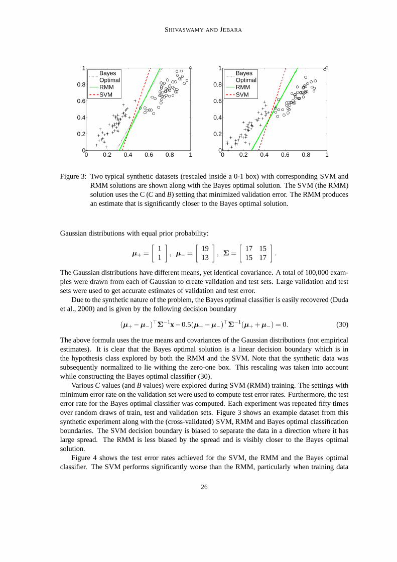
Figure 3: Two typical synthetic datasets (rescaled inside a0-1 box) with corresponding SVM andRMM solutions are shown along with the Bayes optimal solution. The SVM (the RMM)solution uses the C (C andB) setting that minimized validation error. The RMM producesan estimate that is significantly closer to the Bayes optimalsolution.
Gaussian distributions with equal prior probability:
µ+ =
[
11
]
, µ− =
[
1913
]
, Σ =
[
17 1515 17
]
.
The Gaussian distributions have different means, yet identical covariance. A total of 100,000 exam-ples were drawn from each of Gaussian to create validation and test sets. Large validation and testsets were used to get accurate estimates of validation and test error.
Due to the synthetic nature of the problem, the Bayes optimalclassifier is easily recovered (Dudaet al., 2000) and is given by the following decision boundary
(µ+ −µ−)⊤Σ−1x−0.5(µ+ −µ−)⊤Σ
−1(µ+ +µ−) = 0. (30)
The above formula uses the true means and covariances of the Gaussian distributions (not empiricalestimates). It is clear that the Bayes optimal solution is a linear decision boundary which is inthe hypothesis class explored by both the RMM and the SVM. Note that the synthetic data wassubsequently normalized to lie withing the zero-one box. This rescaling was taken into accountwhile constructing the Bayes optimal classifier (30).
VariousC values (andB values) were explored during SVM (RMM) training. The settings withminimum error rate on the validation set were used to computetest error rates. Furthermore, the testerror rate for the Bayes optimal classifier was computed. Each experiment was repeated fifty timesover random draws of train, test and validation sets. Figure3 shows an example dataset from thissynthetic experiment along with the (cross-validated) SVM, RMM and Bayes optimal classificationboundaries. The SVM decision boundary is biased to separatethe data in a direction where it haslarge spread. The RMM is less biased by the spread and is visibly closer to the Bayes optimalsolution.
Figure 4 shows the test error rates achieved for the SVM, the RMM and the Bayes optimalclassifier. The SVM performs significantly worse than the RMM, particularly when training data
26

MAXIMUM RELATIVE MARGIN AND DATA -DEPENDENTREGULARIZATION
102
103
104
0.8
0.9
1
1.1
# train
Tes
t err
or
SVMRMMBayesOptimal
Figure 4: Percent test error rates for the SVM, RMM and Bayes optimal classifier as training datasize is increased. The RMM has a statistically significant (at 5% level) advantage overthe SVM until 6400 training examples. Subsequently, the advantage remains though withless statistical significance.
is scarce. The RMM maintains a statistically significant advantage over the SVM until the numberof training examples grows beyond 6400. With larger training sample sizen, regularization playsa smaller role in the future probability of error. This is clear, for instance, from the bound (27).The last term goes to zero atO(1/
√n), the second term (which is the outcome of regularization)
is O(√
tr(K)/n√
1/n). Both have anO(1/√
n) rate. However, the first term in the bound is theaverage slack variables divided by the margin which does notgo to zero asymptotically with in-creasingn and eventually dominates the bound. Thus, the SVM and RMM have asymptoticallysimilar performance but have significant differences in thesmall sample case.
The effect of scaling, which is a particular affine transformation, was explored next. To explorethe effect of scaling in a controlled manner, first, the projection w recovered by the Bayes optimalclassifier was obtained. An orthogonal vectorv (such thatw⊤v = 0) was then obtained. The ex-amples (training, test and validation) were then projectedonto the axes defined byw andv. Eachprojection alongw was preserved while the projection alongv was scaled by a factors> 1. Thismerely elongates the data further along directions orthogonal to w (i.e, along the Bayes optimalclassification boundary). More concisely, given an examplex, the following scaling transformationwas applied:
[
w v]
[
1 00 s
]
[
w v]−1
x. (31)
Figure 5 shows the SVM and RMM test error rate across a range ofscaling valuess. Here, 100examples were used to construct the training data. Ass grows, the SVM further deviates from the
27

SHIVASWAMY AND JEBARA
0 5 10 15 20
0.8
1
1.2
1.4
scaling s
Tes
t err
or
SVM
RMMBayesOptimal
Figure 5: Percent test error rates for the SVM, RMM and Bayes optimal classifier as data is scaledaccording to (31). The RMM solution remains resilient to scaling while the SVM solu-tion deteriorates significantly. The advantage of the RMM over the SVM is statisticallysignificant (at the 1% level).
Bayes optimal classifier and attempts to separate the data along directions of large spread. Mean-while, the RMM remains resilient to scaling and maintains a low error rate throughout.
To explore the effect of theB parameter, the average validation and test error rate were computedacross many settings ofC andB. The settingC = 100 was chosen since it obtained the minimumerror rate on the validation set. The average test error rateof the RMM is shown in Figure 6 atC = 100 for multiple settings of theB parameter. Starting from the SVM solution on the right(i.e. largeB) the error rate begins to fall until it attains a minimum and then starts to go increase.A similar behavior is seen in many real world datasets. Surprisingly, some datasets even exhibitmonotonic reduction in test error as the value ofB is decreased. The following section investigatessuch real world experiments in more detail.
5.2 Experiments on digits
Experiments were carried out on three datasets of digits - optical digits from the UCI machinelearning repository (Asuncion and Newman, 2007), USPS digits (LeCun et al., 1989) and MNISTdigits (LeCun et al., 1998). These datasets vary considerably in terms of their number of features(64 in optical digits, 256 in USPS and 784 in MNIST) and their number of training examples (3823in optical digits, 7291 in USPS and 60000 in MNIST). In all themulti-class experiments, the oneversus one classification strategy was used. The one versus one strategy trains a classifier for everycombination of two classes. The final prediction for an example is simply the class that is predictedmost often. These results are directly comparable with various methods that have been applied on
28
MAXIMUM RELATIVE MARGIN AND DATA -DEPENDENTREGULARIZATION
1
1.2
1.4A
vera
ge E
rror
Rat
e
SVM
Decreasing B
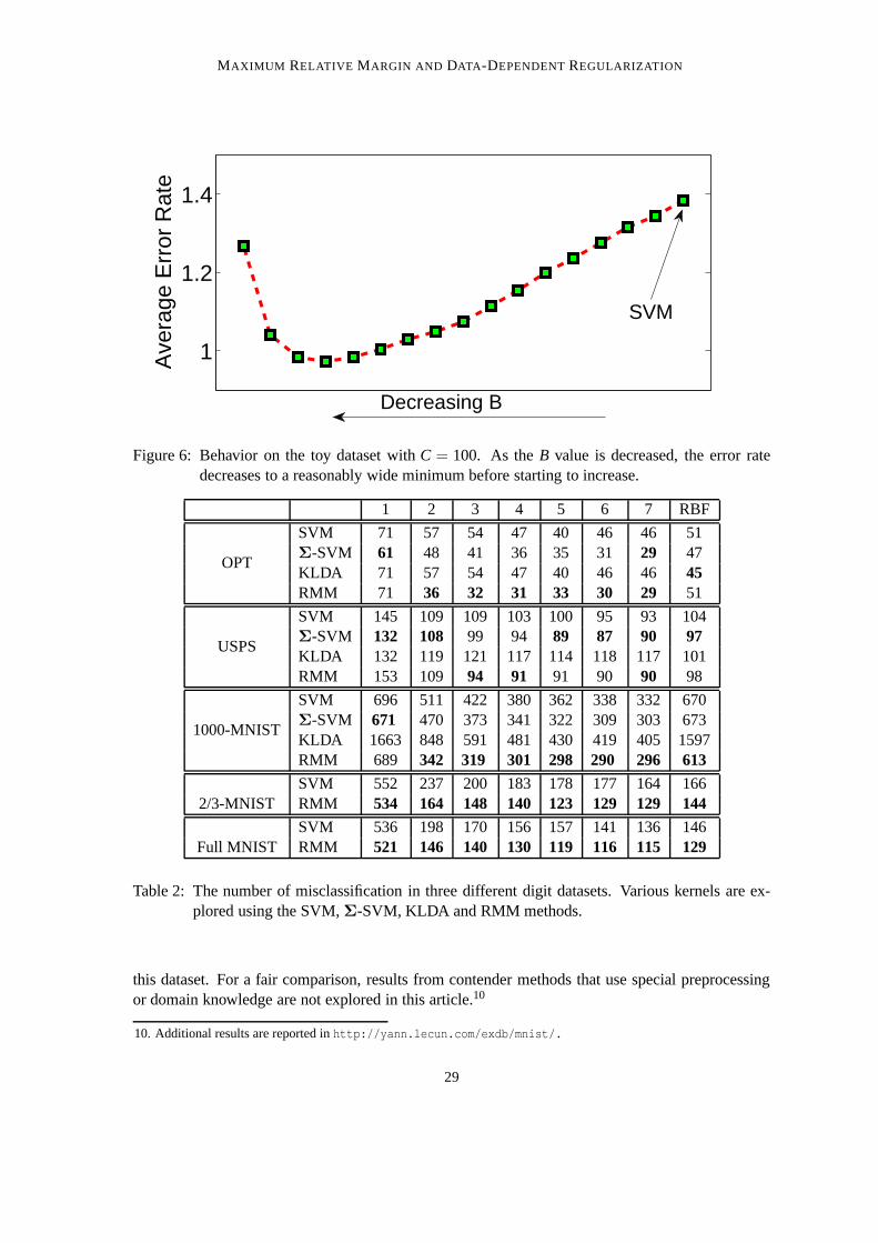
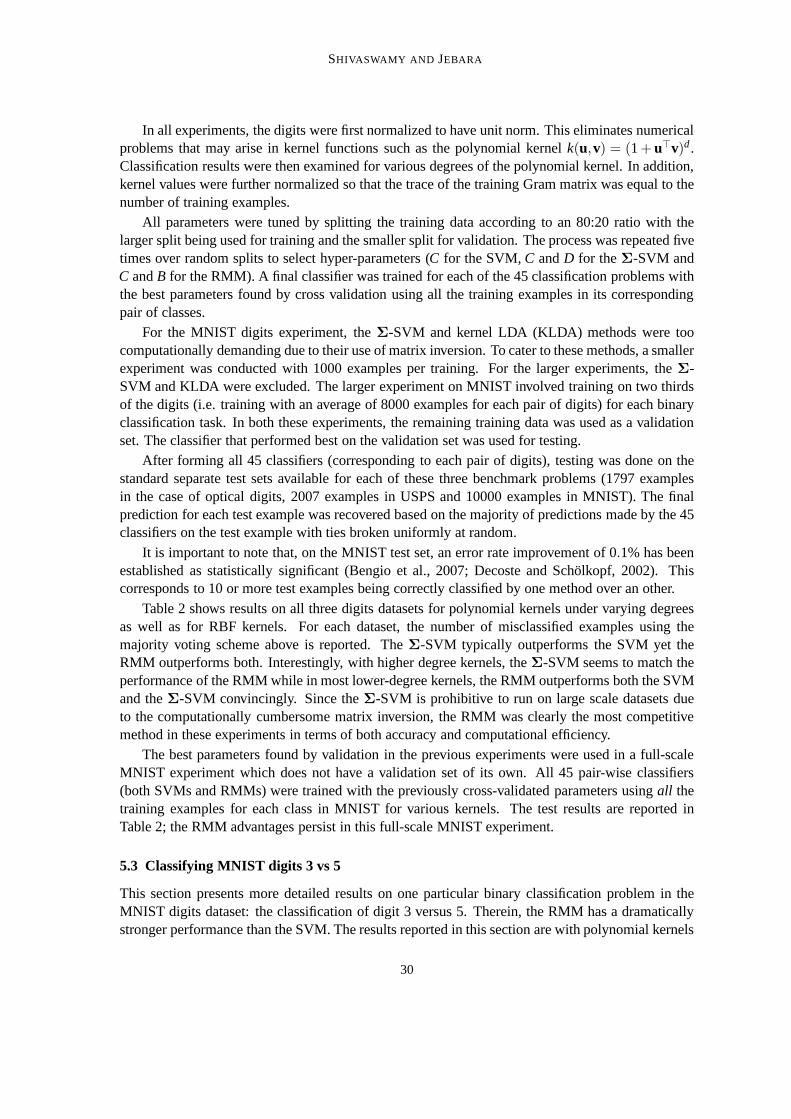
Figure 6: Behavior on the toy dataset withC = 100. As theB value is decreased, the error ratedecreases to a reasonably wide minimum before starting to increase.
1 2 3 4 5 6 7 RBF
OPT
SVM 71 57 54 47 40 46 46 51Σ-SVM 61 48 41 36 35 31 29 47KLDA 71 57 54 47 40 46 46 45RMM 71 36 32 31 33 30 29 51
USPS
SVM 145 109 109 103 100 95 93 104Σ-SVM 132 108 99 94 89 87 90 97KLDA 132 119 121 117 114 118 117 101RMM 153 109 94 91 91 90 90 98
1000-MNIST
SVM 696 511 422 380 362 338 332 670Σ-SVM 671 470 373 341 322 309 303 673KLDA 1663 848 591 481 430 419 405 1597RMM 689 342 319 301 298 290 296 613
2/3-MNISTSVM 552 237 200 183 178 177 164 166RMM 534 164 148 140 123 129 129 144
Full MNISTSVM 536 198 170 156 157 141 136 146RMM 521 146 140 130 119 116 115 129
Table 2: The number of misclassification in three different digit datasets. Various kernels are ex-plored using the SVM,Σ-SVM, KLDA and RMM methods.
this dataset. For a fair comparison, results from contendermethods that use special preprocessingor domain knowledge are not explored in this article.10
10. Additional results are reported inhttp://yann.lecun.com/exdb/mnist/.
29
SHIVASWAMY AND JEBARA
In all experiments, the digits were first normalized to have unit norm. This eliminates numericalproblems that may arise in kernel functions such as the polynomial kernelk(u,v) = (1+ u⊤v)d.Classification results were then examined for various degrees of the polynomial kernel. In addition,kernel values were further normalized so that the trace of the training Gram matrix was equal to thenumber of training examples.
All parameters were tuned by splitting the training data according to an 80:20 ratio with thelarger split being used for training and the smaller split for validation. The process was repeated fivetimes over random splits to select hyper-parameters (C for the SVM,C andD for theΣ-SVM andC andB for the RMM). A final classifier was trained for each of the 45 classification problems withthe best parameters found by cross validation using all the training examples in its correspondingpair of classes.
For the MNIST digits experiment, theΣ-SVM and kernel LDA (KLDA) methods were toocomputationally demanding due to their use of matrix inversion. To cater to these methods, a smallerexperiment was conducted with 1000 examples per training. For the larger experiments, theΣ-SVM and KLDA were excluded. The larger experiment on MNIST involved training on two thirdsof the digits (i.e. training with an average of 8000 examplesfor each pair of digits) for each binaryclassification task. In both these experiments, the remaining training data was used as a validationset. The classifier that performed best on the validation setwas used for testing.
After forming all 45 classifiers (corresponding to each pairof digits), testing was done on thestandard separate test sets available for each of these three benchmark problems (1797 examplesin the case of optical digits, 2007 examples in USPS and 10000examples in MNIST). The finalprediction for each test example was recovered based on the majority of predictions made by the 45classifiers on the test example with ties broken uniformly atrandom.
It is important to note that, on the MNIST test set, an error rate improvement of 0.1% has beenestablished as statistically significant (Bengio et al., 2007; Decoste and Scholkopf, 2002). Thiscorresponds to 10 or more test examples being correctly classified by one method over an other.
Table 2 shows results on all three digits datasets for polynomial kernels under varying degreesas well as for RBF kernels. For each dataset, the number of misclassified examples using themajority voting scheme above is reported. TheΣ-SVM typically outperforms the SVM yet theRMM outperforms both. Interestingly, with higher degree kernels, theΣ-SVM seems to match theperformance of the RMM while in most lower-degree kernels, the RMM outperforms both the SVMand theΣ-SVM convincingly. Since theΣ-SVM is prohibitive to run on large scale datasets dueto the computationally cumbersome matrix inversion, the RMM was clearly the most competitivemethod in these experiments in terms of both accuracy and computational efficiency.
The best parameters found by validation in the previous experiments were used in a full-scaleMNIST experiment which does not have a validation set of its own. All 45 pair-wise classifiers(both SVMs and RMMs) were trained with the previously cross-validated parameters usingall thetraining examples for each class in MNIST for various kernels. The test results are reported inTable 2; the RMM advantages persist in this full-scale MNISTexperiment.
5.3 Classifying MNIST digits 3 vs 5
This section presents more detailed results on one particular binary classification problem in theMNIST digits dataset: the classification of digit 3 versus 5.Therein, the RMM has a dramaticallystronger performance than the SVM. The results reported in this section are with polynomial kernels
30

MAXIMUM RELATIVE MARGIN AND DATA -DEPENDENTREGULARIZATION
0
2
4
6
8
10
12
14
16
Decreasing B
Tes
t Err
ors
3 VS 5
SVM
Figure 7: Performance on MNIST test set with digits 3 and 5. The number of errors decreases from15 to 6 asB decreases from the right.
of degree 5. The parameterC was selected as mentioned above. With the selectedC value, an SVMwas first trained over the entire MNIST training set containing the digits 3 and 5. After noting themaximum absolute value of the output given on all the training examples,B value was reduced insteps. The number of test errors on the MNIST test set (3 versus 5) was noted. As theB valueis reduced, the number of errors starts to diminish as shown in Figure 7. The number of errorsproduced by the SVM was 15. With the RMM, the number of errors dropped to 6 as theB valueapproached one. Clearly, asB decreases, the absolute margin is decreased however the test errorrate drops drastically. This empirically suggests that maximizing the relative margin can have abeneficial effect on the performance of a classifier. Admittedly, this is only one example and isprovided only for illustrative purposes. However, similarbehavior was observed in most of thebinary digit classification problems though in some cases the error rate did not go down significantlywith decreasingB values. The generalization behavior on all 45 individual problems is explored inmore detail in Section 5.4.
5.4 All 45 binary MNIST problems
This section explores RMM performance on the 45 pairwise digit classification problems in isola-tion. In these experiments, bothC andB values were fixed using validation as in previous sections.A total of 45 binary classifiers were constructed using all MNIST training digits. The resulting errorrates are shown in Figure 8. On most problems, the RMM obtainsa significantly lower error ratethan the SVM and, at times obtains half the error rate.
31

SHIVASWAMY AND JEBARA
0 5 10 15 20 25 30 35 40 450
2
4
6
8
10
12
14
16
18
45 Individual Problems
Err
or
SVM
RMM
Figure 8: Total test errors on all 45 MNIST classification problems. Various classifiers were trainedon the entire MNIST training dataset and evaluated on a standardized separate test set.
Method RMM U-SVM# Universum - 1000 3000 allError rate 1.081 1.059 1.037 1.020Error Std Dev 0.138 0.142 0.149 0.159p-value 0.402 0.148 0.031
Table 3: Percentage error rates for the RMM and theU-SVM. The rate for the SVM was 1.274 witha standard deviation of 0.179; this is significantly larger than all other results in the table(with a p-value of 0.000). The final row reports the p-value of a paired t-test between theRMM error rate and theU-SVM error rate (corresponding to the Universum size beingconsidered in that column).
5.4.1 A COMPARISON WITH THEUNIVERSUM METHOD
A new framework known as the Universum (Weston et al., 2006; Sinz et al., 2008) was recentlyintroduced which maximizes the margin while keeping classifier outputs low on an additional col-lection of non-examples that do not belong to either class ofinterest. These additional examplesare known as Universum examples. Like landmarks, these are examples where a classifier’s scalarpredictions are forced to remain small. However, these Universum examples are obtained from anyother distribution other than the one generating the training data. In the RMM, classification outputson training examples are bounded; in the Universum, classification outputs on Universum examplesare bounded (albeit with a different loss). The following experiments compare the Universum basedframework with the RMM.
32
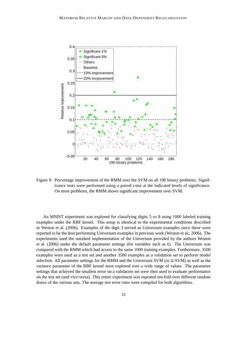
MAXIMUM RELATIVE MARGIN AND DATA -DEPENDENTREGULARIZATION
20 40 60 80 100 120 140 160 180−0.05
0
0.05
0.1
0.15
0.2
0.25
0.3
0.35
0.4
190 binary problems
Rel
ativ
e im
prov
emen
t
Significant 1%
Significant 5%
Others
Baseline
10% improvement
20% imrpovement
Figure 9: Percentage improvement of the RMM over the SVM on all 190 binary problems. Signif-icance tests were performed using a paired t-test at the indicated levels of significance.On most problems, the RMM shows significant improvement overSVM.
An MNIST experiment was explored for classifying digits 5 vs8 using 1000 labeled trainingexamples under the RBF kernel. This setup is identical to theexperimental conditions describedin Weston et al. (2006). Examples of the digit 3 served as Universum examples since these werereported to be thebestperforming Universum examples in previous work (Weston et al., 2006). Theexperiments used the standard implementation of the Universum provided by the authors Westonet al. (2006) under the default parameter settings (for variables such asε). The Universum wascompared with the RMM which had access to the same 1000 training examples. Furthermore, 3500examples were used as a test set and another 3500 examples as avalidation set to perform modelselection. All parameter settings for the RMM and the Universum SVM (orU-SVM) as well as thevariance parameter of the RBF kernel were explored over a wide range of values. The parametersettings that achieved the smallest error on a validation set were then used to evaluate performanceon the test set (and vice-versa). This entire experiment wasrepeated ten-fold over different randomdraws of the various sets. The average test error rates were compiled for both algorithms.
33

SHIVASWAMY AND JEBARA
While the RMM only had access to the 1000 training examples, the U-SVM was also givena Universum of images of the digit 3. The Universum spanned three different sizes - 1000, 3000and 6131 examples (i.e. all available images of the digit 3 inthe MNIST training set). The resultsare reported in Table 3. First, observe that both the RMM and theU-SVM improved the baselineSVM performance significantly (as measured by a paired t-test). With 1000 and 3000 Universumexamples, even though the error rate of theU-SVM was slightly lower, a paired t-test revealedthat it did not achieve statistically significant improvement over the RMM. Statistically significantadvantages for theU-SVM only emerged whenall the available images of the digit 3 were used inthe Universum.
Note that there is a slight discrepancy between the errors reported here and those in Westonet al. (2006) even though both methods used the digit 3 to generate Universum examples. This maybe because the previous authors Weston et al. (2006) reported thebest test erroron 1865 examples.In this article, a more conservative approach is taken wherea good model is first selected usingthe validation set and then errors are reported on an unseen test set without further tuning. Clearly,picking the minimum error rate on a test set will give more optimistic results but tuning to the test setcan be potentially misleading. This makes it difficult to directly compare test error rates with thosereported in the previous paper. While the error rate (using all digits 3 as the Universum examples) inour experiments varied from 0.74% to 1.35%, the authors in Weston et al. (2006) reported an errorrate of 0.62%.
With 1000 training examples, the RMM (as in Equation (8)) has1000 classification constraintsand 1000 bounding constraints. With 1000 Universum examples, theU-SVM also has 1000 bound-ing constraints in addition to the classification constraints. It is interesting to note that the RMM,with no extra data, is not significantly worse than aU-SVM endowed with an additional 1000 or3000best-possibleUniversum examples.
The authors of Weston et al. (2006) observed that Universum examples help most when theyare correlated with the training examples. This, coupled with the results in Table 3 and the fact thattraining examples are correlated most with themselves (or with examples from the same distributionas the training examples), raises the following question: How much of the performance gain withthe U-SVM is due to the extra examples and how much of it is due to itsimplicit control of thespread (as with an RMM)? This is left as an open question in this article and as motivation forfurther theoretical work.
5.5 Text classification
In this section, results are reported on the 20 Newsgroups11 dataset. This dataset has posts from 20different Usenet newsgroups. Each post was represented by avector which counts the number ofwords that occurred in the document. In the text classification literature, this is commonly knownas the bag of words representation. Each feature vector was divided by the total number of words inthe document to normalize it.
All 190 binary pairwise classification problems were considered in this experiment. For eachproblem, 500 examples were used for training. The remainingexamples were divided into a valida-tion and test set of the same size. Both SVMs and RMMs were trained for various values of theirparameters. After finding the parameter settings that achieved the lowest error on a validation set,
11. This dataset is available online athttp://people.csail.mit.edu/jrennie/20Newsgroups/.
34

MAXIMUM RELATIVE MARGIN AND DATA -DEPENDENTREGULARIZATION
the test error was evaluated (and vice-versa). This experiment was repeated ten times for randomdraws of the train, validation and test sets.
Figure 9 summarizes the results. For each binary classification problem, a paired t-test wasperformed and p-values were obtained. As can be seen from theplot, the RMM outperforms theSVM significantly in almost 30% of the problems. This experiment once again demonstrates thatan absolute margin does not always result in a small test error.
3.6 3.8 4 4.2 4.4 4.6 4.8 5 5.21.5
2
2.5
3
3.5
4
4.5
Log # examples
Log
runt
ime
SVMRMM, B_1RMM, B_2RMM, B_3
Figure 10: Log run time versus log number of examples. The figure shows that the SVM and theRMM have similar computational requirements overall.
35

SHIVASWAMY AND JEBARA
Dataset SVM KFDA Σ-SVM RMM (C=D) RMMbanana 10.5± 0.4 10.8± 0.5 10.5± 0.4 10.4± 0.4 10.4± 0.4*b.cancer 25.3± 4.6* 26.6± 4.8 28.8± 4.6 25.9± 4.5 25.4± 4.6diabetes 23.1± 1.7 23.2± 1.8 24.2± 1.9 23.1± 1.7 23.0± 1.7*f.solar 32.3± 1.8 33.1± 1.6 34.6± 2.0 32.3± 1.8* 32.3± 1.8*German 23.4± 2.2 24.1± 2.4 25.9± 2.4 23.4± 2.1 23.2± 2.2*heart 15.5± 3.3 15.7± 3.2 19.9± 3.6 15.4± 3.3 15.2± 3.1*image 3.0± 0.6 3.1± 0.6 3.3± 0.7 3.0± 0.6 2.9± 0.7ringnorm 1.5± 0.1 1.5± 0.1 1.5± 0.1 1.5± 0.1 1.5± 0.1*splice 10.9± 0.7 10.6± 0.7 10.8± 0.6 10.8± 0.6 10.8± 0.6thyroid 4.7± 2.1 4.2± 2.1 4.5± 2.1 4.2± 1.8* 4.2± 2.2titanic 22.3± 1.1 22.0± 1.3* 23.1± 2.2 22.3± 1.1 22.3± 1.0twonorm 2.4± 0.1* 2.4± 0.2 2.5± 0.2 2.4± 0.1 2.4± 0.1waveform 9.9± 0.4 9.9± 0.4 10.5± 0.5 10.0± 0.4 9.7± 0.4*
Dataset RBF AB LPAB QPAB ABRbanana 10.8± 0.4 12.3± 0.7 10.7± 0.4 10.9± 0.5 10.9± 0.4b.cancer 27.6± 4.7 30.4± 4.7 26.8± 6.1 25.9± 4.6 26.5± 4.5diabetes 24.3± 1.9 26.5± 2.3 24.1± 1.9 25.4± 2.2 23.8± 1.8f.solar 34.4± 1.9 35.7± 1.8 34.7± 2.0 36.2± 1.8 34.2± 2.2German 24.7± 2.4 27.5± 2.5 24.8± 2.2 25.3± 2.1 24.3± 2.1heart 17.1± 3.3 20.3± 3.4 17.5± 3.5 17.2± 3.4 16.5± 3.5image 3.3± 0.7 2.7± 0.7 2.8± 0.6 2.7± 0.6* 2.7± 0.6*ringnorm 1.7± 0.2 1.9± 0.2 2.2± 0.5 1.9± 0.2 1.6± 0.1splice 9.9± 0.8 10.1± 0.5 10.2± 1.6 10.1± 0.5 9.5± 0.6*thyroid 4.5± 2.1 4.4± 2.2 4.6± 2.2 4.3± 2.2 4.5± 2.2titanic 23.3± 1.3 22.6± 1.2 24.0± 4.4 22.7± 1.0 22.6± 1.2twonorm 2.8± 0.3 3.0± 0.3 3.2± 0.4 3.0± 0.3 2.7± 0.2waveform 10.7± 1.1 10.8± 0.6 10.5± 1.0 10.1± 0.5 9.8± 0.8
Table 4: UCI results for a number of classification methods. Results are shown for the SVM, reg-ularized kernel Fisher Discriminant Analysis, theΣ-SVM, the RMM, an RBF network,Adaboost, LP-regularized Adaboost, QP-regularized Adaboost and Regularized Adaboost.The results have been split into two parts due to lack of space. For each dataset, all meth-ods could be placed on the same row in a larger table. For each dataset, the algorithmwhich gave the minimum error rate is starred. All other algorithms that were not signifi-cantly different from (at the 5% significance level based on apaired t-test) the minimumerror rate are in boldface.
36

MAXIMUM RELATIVE MARGIN AND DATA -DEPENDENTREGULARIZATION
5.6 Benchmark datasets
To compare the performance of the RMM with a number of other methods, experiments were per-formed on several benchmark datasets. In particular, 100 training and test splits of 13 of thesedatasets have been previously used in (Raetsch et al., 2001;Mika et al., 1999; Cawley and Talbot,2003).12 The RBF kernel was used in these experiments for all kernel-based methods. To handle thenoisy nature of these datasets, the kernelized and relaxed version of the RMM (14) was used. Allthe parameters were tuned using cross-validation using a similar setup as in (Raetsch et al., 2001)13.With the chosen values of these parameters, the error rates were first obtained for all 100 test splitsusing the corresponding training splits. The results are reported in Table 4. Once again, the RMMexhibits clear performance advantages over other methods.
5.7 Scalability and run-time
While the asymptotic run time behavior was analyzed in Section 3.3, the run time of the RMM isalso studied empirically in this section. In particular, the classification of MNIST digits 0-4 versus5-9 with a polynomial kernel of degree five was used to benchmark the algorithms. For both theRMM and the SVM, the tolerance parameter (ε mentioned in Section 3.3) was set to 0.001. The sizeof the sub-problem (12) solved was 800 in all the cases. To evaluate how the algorithms scale, thenumber of training examples was increased in steps and the training time was noted. Throughoutall the experiments, theC value was set to 1. The SVM was first run on the training examples. Thevalue of maximum absolute predictionθ was noted. Three different values ofB were then tried forthe RMM:B1 = 1+(θ−1)/2, B2 = 1+(θ−1)/4 andB3 = 1+(θ−1)/10. In all experiments, therun time was noted. The experiment was repeated ten times to get an average run time for eachBvalue. A log-log plot comparing the number of examples to theaverage run time is shown in Figure10. Both the SVM and the RMM run time exhibit similar asymptotic behavior.
6. Conclusions
The article showed that support vector machines and maximummargin classifiers can be sensitiveto affine transformations of the input data and are biased in favor of separating data along directionswith large spread. The relative margin machine was proposedto overcome such problems and op-timizes the projection direction such that the margin is large onlyrelative tothe spread of the data.By deriving the dual with quadratic constraints, a geometric interpretation was also formulated forRMMs and led to risk bounds via Rademacher complexity arguments. In practice, the RMM imple-mentation requires only additional linear constraints that complement the SVM quadratic programand maintain its efficient run time. Empirically, the RMM andmaximum relative margin approachshowed significant improvements in classification accuracy. In addition, an intermediate methodknown asΣ-SVM was shown that lies between the SVM and the RMM both conceptually and interms of classification performance.
Generalization bounds with Rademacher averages were derived. The SVM’s bound which in-volves the trace of the kernel matrix was replaced with a moregeneral whitened version of the traceof the kernel matrix. A proof technique using landmark examples led to Rademacher bounds on an
12. These datasets are available athttp://theoval.cmp.uea.ac.uk/∼gcc/matlab/default.html#benchmarks.13. The values of the selected parameters and the code for theRMM are available for download at
http://www.cs.columbia.edu/∼pks2103/ucirmm/.
37

SHIVASWAMY AND JEBARA
empirical data-dependent hypothesis space. Furthermore,the bounds were stated independently ofthe particular sample of landmarks.
Directions of future work include exploring the connections between maximum relative marginand generalization bounds based on margin distributions (Schapire et al., 1998; Koltchinskii andPanchenko, 2002). By bounding outputs, the RMM is potentially finding a better margin distributionon the training examples. Previous arguments for such an approach were obtained in the context ofvoting methods (such as boosting) and may also be relevant here.
Furthermore, the maximization of relative margin is a fairly promising and general conceptwhich may be compatible with other popular problems that have recently been tackled by the max-imum margin paradigm. These include regression, ordinal regression, ranking and so forth. Theseare valuable and natural extensions for the RMM. Finally, since the constraints that bound the pro-jections are unsupervised, RMMs can readily apply in semi-supervised and transductive settings.These are all promising directions for future work.
Acknowledgement
This material is based in part upon work supported by the National Science Foundation under GrantNumber IIS-0347499. Any opinions, findings, and conclusions or recommendations expressed inthis material are those of the authors and do not necessarilyreflect the views of the National ScienceFoundation.
Appendix A. McDiarmid’s inequality
AssumeX1,X2, . . . ,Xn are independent random variables from a setX and g : X n → R. If thefunction g satisfies supX1,...,Xn,Xk
|g(X1, . . . ,Xn)−g(X1, . . . , Xk, . . . ,Xn)| ≤ ck, for all 1≤ k ≤ n then,for anyε > 0:
Pr[g(X1, . . . ,Xn)−E[g(X1, . . . ,Xn)] ≥ ε] ≤ exp
(
− 2ε2
∑ni=1 c2
i
)
, (32)
Pr[E[g(X1, . . . ,Xn)]−g(X1, . . . ,Xn) ≥ ε] ≤ exp
(
− 2ε2
∑ni=1 c2
i
)
,
where the expectations are over the random draws ofX1, . . . ,Xn. Here the constantsc1,c2, · · · ,cn arecalled Lipschitz constants.
Appendix B. Lipschitz constants for Section 4.6
Lemma 19 The upper bound onR(GUB,D), namely T1(U,S), admits the Lipschitz constant:
2√
2BDn
(√
n
∑i=1
x⊤i xi −√
n
∑i=1
x⊤i xi −DR2µmax
nD+DR2
)
.
Proof The quantity of interest is the worst change in
2√
2Bn
√
n
∑i=1
xi(DI +Dn
n
∑j=1
u ju⊤j )−1x⊤i
38

MAXIMUM RELATIVE MARGIN AND DATA -DEPENDENTREGULARIZATION
whenuk is varied for any setting ofu1, . . . ,uk−1,uk+1, . . . ,un. Since∑nj=1, j 6=k u ju⊤
j is positive semi-definite and inside the inverse operator,uk will have the most extreme effect on the expression when∑n
j=1, j 6=k u ju⊤j = 0. Thus, consider:
2√
2Bn
√
n
∑i=1
x⊤i
(
DI +Dn
uku⊤k
)−1
xi .
Apply the Woodbury matrix inversion identity to the term inside the square root:
n
∑i=1
x⊤i
(
DI +Dn
uku⊤k
)−1
xi =1D
n
∑i=1
x⊤i
(
I − uku⊤k
nDD +u⊤
k uk
)
xi
=1D
(
n
∑i=1
x⊤i xi − ∑ni=1(x
⊤i uk)
2
nDD +u⊤
k uk
)
.
The maximum value of this expression occurs whenuk = 0. To find the minimum, write the secondterm inside the brackets in the above expression as below:
(
u⊤k
‖uk‖n
∑i=1
xix⊤iuk
‖uk‖
)
/
(
nD
Du⊤k uk
+1
)
.
Clearly, in the numerator, the magnitude ofuk does not matter. To maximize this expression,uk
should be set to a vector of maximal length and in the same direction as the maximum eigenvectorof ∑n
i=1 xix⊤i . Since all examples are assumed to have bounded norm no larger thanR, the largestuk
vector has normR. Denoting the maximum eigenvalue of∑ni=1 xix⊤i by µmax, it is easy to show the
claimed value of Lipschitz constant for anyk.
Lemma 20 The upper bound onR(H VE,D), namely T2(V,S), admits the Lipschitz constant:
2√
2EDn
(√
n
∑i=1
x⊤i xi −√
n
∑i=1
x⊤i xi −DR2µmax
nD+DR2
)
.
Proof The quantity of interest is the maximum change in the following optimization problem overuk for any setting ofu1,u2, . . . ,uk−1,uk+1, . . . ,unv :
minλ≥0
1n
n
∑i=1
x⊤i
(
Dnv
∑j=1
λ j I +Dnv
∑j=1
λ ju ju⊤j
)−1
xi +2n
Env
∑i=1
λi .
As before, this happens when allu’s exceptuk are0. In such a scenario, the expression is minimizedfor the settingλ j = 0 for all j 6= k. The minimization only needs to consider variable settingsof λk.Since this minimization is over a single scalar, it is possible to obtain a closed-form expression for
λk. The optimalλk is merely: 1√2E ∑n
i=1 x⊤i(
DI +Duku⊤k
)−1xi . Substituting this into the objective
gives an expression which is independent ofλ’s:
2√
2En
√
n
∑i=1
x⊤i
(
DI +Dn
uku⊤k
)−1
xi .
This expression is identical to the one obtained in Theorem 19 and the proof follows.
39

SHIVASWAMY AND JEBARA
Appendix C. Solving for nv
Letx= 1√nv
,c= 4R√
2ED andb= 3
2
√
ln (2/δ)2 . Consider solving forx in the expressionx2−2bx= (c+
2b)/√
n. Equivalently, solve(x−b)2 = b2+(c+2b)/√
n. Taking the square root of both sides givesx = b±
√
b2 +(c+2b)/√
n. Sincex > 0, only the positive root is considered. Thus,√
nv = 1/(b+√
b2 +(c+2b)/√
n) which gives an exact expression fornv. Dropping terms from the denominator
produces the simpler expression:√
nv ≤ 1/√
(c+2b)/√
n. Hence,nv ≤√
n
4R√
2ED +3
√
ln(2/δ)2
.
References
A. Asuncion and D.J. Newman. UCI machine learning repository, 2007.
P. L. Bartlett and S. Mendelson. Rademacher and Gaussian complexities: Risk bounds and structuralresults.Journal of Machine Learning Research, 3:463–482, 2002.
M. Belkin, P. Niyogi, and V. Sindhwani. On manifold regularization. InArtificial Intelligence andStatistics, 2005.
Y. Bengio, P. Lamblin, D. Popovici, and H. Larochelle. Greedy layer-wise training of deep networks.In B. Scholkopf, J. Platt, and T. Hoffman, editors,Advances in Neural Information ProcessingSystems 19, pages 153–160. MIT Press, Cambridge, MA, 2007.
O. Bousquet, S. Boucheron, and G. Lugosi. Introduction to statistical learning theory. InLectureNotes in Artificial Intelligence 3176, pages 169–207, Heidelberg, Germany, 2004. Springer.
S. Boyd and L. Vandenberghe.Convex Optimization. Cambridge University Press, 2003.
G. C. Cawley and N. L. C Talbot. Efficient leave-one-out cross-validation of kernel fisher discrimi-nant classifiers.Pattern Recognition, 36:2585–2592, 2003.
N. Cesa-Bianchi, A. Conconi, and C. Gentile. A second-orderperceptron algorithm.SIAM J.Comput., 34(3):640–668, 2005.
M. Collins and B. Roark. Incremental parsing with the perceptron algorithm. InAnnual Meeting ofthe Association for Computational Linguistics, pages 111–118, 2004.
K. Crammer, M. Dredze, and F. Pereira. Exact convex confidence-weighted learning. InAdvancesin Neural Information Processing Systems 21, Cambridge, MA, 2009a. MIT Press.
K. Crammer, M. Mohri, and F. Pereira. Gaussian margin machines. InProceedings of the ArtificialIntelligence and Statistics, 2009b.
D. Decoste and B. Scholkopf. Training invariant support vector machines.Machine Learning, pages161–190, 2002.
M. Dredze, K. Crammer, and F. Pereira. Confidence-weighted linear classification. InInternationcalConference on Machine Leaarning, 2008.
40

MAXIMUM RELATIVE MARGIN AND DATA -DEPENDENTREGULARIZATION
R. O. Duda, P. E. Hart, and D. G. Stork.Pattern Classification. Wiley-Interscience Publication,2000.
P. Haffner. Escaping the convex hull with extrapolated vector machines. In T. G. Dietterich,S. Becker, and Z. Ghahramani, editors,Advances in Neural Information Processing Systems 14,pages 753–760. MIT Press, Cambridge, MA, 2001.
R. Herbrich, T. Graepel, and C. Campbell. Bayes point machines. Journal of Machine LearningResearch, 1:245–279, 2001.
T. Jaakkola, M. Meila, and T. Jebara. Maximum entropy discrimination. InAdvances in NeuralInformation Processing Systems 11, 1999.
T. Joachims. Transductive inference for text classification using support vector machines. InPro-ceedings of the 16th International Conference on Machine Learning, 1999.
T. Joachims. Training linear SVMs in linear time. InACM SIGKDD International Conference OnKnowledge Discovery and Data Mining (KDD), pages 217–226, 2006.
T. Joachims. Making large-scale support vector machine learning practical. In A. SmolaB. Scholkopf, C. Burges, editor,Advances in Kernel Methods: Support Vector Machines. MITPress, Cambridge, MA, 1998.
S.S. Keerthi. Efficient tuning of svm hyperparameters usingradius/margin bound and iterativealgorithms.IEEE Transactions on Neural Networks, 13:1225–1229, 2002.
V. Koltchinskii and D. Panchenko. Empirical margin distributions and bounding the generalizationerror of combined classifiers.Annals of Statistics, 30, 2002.
Y. LeCun, B. Boser, J.S. Denker, D. Henderson, R.E. Howard, W. Hubbard, and L. Jackel. Back-propagation applied to handwritten zip code recognition.Neural Computation, 1:541–551, 1989.
Y. LeCun, L. Bottou, Y. Bengio, and P. Haffner. Gradient-based learning applied to documentrecognition.Proceedings of the IEEE, 86(11):2278–2324, 1998.
S. Mika, G. Raetsch, J. Weston, B. Scholkopf, and K.-R. Muller. Fisher discriminant analysis withkernels. Inin Neural Networks for Signal Processing IX, pages 41–48, 1999.
G. Raetsch, T. Onoda, and K.-R. Muller. Soft margins for adaboost. Machine Learning, 43:287–320, 2001.
R. E. Schapire, Y. Freund, P. Bartlett, and W. S. Lee. Boosting the margin: a new explanation forthe effectiveness of voting methods.The Annals of Statistics, 26:322–330, 1998.
B. Scholkopf and A.J. Smola.Learning with Kernels. MIT Press, Cambridge, MA, USA, 2002.
S. Shalev-Shwartz, Y. Singer, and N. Srebro. Pegasos: Primal estimated sub-gradient solver forsvm. InInternational Conference on Machine Learning, 2007.
J. Shawe-Taylor and N. Cristianini.Kernel Methods for Pattern Analysis. Cambridge UniversityPress, 2004.
41

SHIVASWAMY AND JEBARA
P. K. Shivaswamy and T. Jebara. Ellipsoidal kernel machines. In Proceedings of the ArtificialIntelligence and Statistics, 2007.
P. K. Shivaswamy and T. Jebara. Relative margin machines. InAdvances in Neural InformationProcessing Systems 21, Cambridge, MA, 2009a. MIT Press.
P. K. Shivaswamy and T. Jebara. Structured prediction with relative margin. InInternational Con-ference on Machine Learning and Applications, 2009b.
P. K. Shivaswamy, C. Bhattacharyya, and A. J. Smola. Second order cone programming approachesfor handling missing and uncertain data.Journal of Machine Learning Research, 7:1283–1314,2006.
F. Sinz, O. Chapelle, A. Agarwal, and B. Scholkopf. An analysis of inference with the univer-sum. In J.C. Platt, D. Koller, Y. Singer, and S. Roweis, editors, Advances in Neural InformationProcessing Systems 20, pages 1369–1376. MIT Press, Cambridge, MA, 2008.
Nathan Srebro, Jason D. M. Rennie, and Tommi S. Jaakola. Maximum-margin matrix factorization.In Advances in Neural Information Processing Systems 17, pages 1329–1336. MIT Press, 2005.
B. Taskar, D. Klein, M. Collins, D. Koller, and C. Manning. Max-margin parsing. InProceedingsof the Conference on Empirical Methods in Natural Language Processing, 2004.
I. Tsochantaridis, T. Joachims, T. Hofmann, and Y. Altun. Large margin methods for structured andinterdependent output variables.Journal of Machine Learning Research, 6:1453–1484, Septem-ber 2005.
V. Vapnik. The Nature of Statistical Learning Theory. Springer Verlag, New York, 1995.
J. Weston, S. Mukherjee, O. Chapelle, M. Pontil, T. Poggio, and V. Vapnik. Feature selection forSVMs. In T. K. Leen, T. G. Dietterich, and V. Tresp, editors,Advances in Neural InformationProcessing Systems 13, pages 668–674. MIT Press, Cambridge, MA, 2000.
J. Weston, R. Collobert, F. H. Sinz, L. Bottou, and V. Vapnik.Inference with the universum. InProceedings of the International Conference on Machine Learning, pages 1009–1016, 2006.
B. Zhang, X. Chen, S. Shan, and W. Gao. Nonlinear face recognition based on maximum averagemargin criterion. InComputer Vision and Pattern Recognition, pages 554–559, 2005.
42
Copyright © 2022 FDOKUMEN