Redefining the Standard Compaction Test to Better Describe ...
126
University of Southern Queensland Faculty of Health Engineering and Sciences Redefining the Standard Compaction Test to Better Describe the Usage of Cotton Picking Machines on Australian Vertosols A Dissertation Submitted By: Mr. Ronald James Wilson 0061032317 In fulfilment of the Requirements of: Bachelor of Engineering
-
Upload
khangminh22 -
Category
Documents
-
view
2 -
download
0
Transcript of Redefining the Standard Compaction Test to Better Describe ...

University of Southern Queensland Faculty of Health Engineering and Sciences
Redefining the Standard Compaction Test to Better Describe the Usage of
Cotton Picking Machines on Australian Vertosols
A Dissertation Submitted By:
Mr. Ronald James Wilson 0061032317
In fulfilment of the Requirements of:
Bachelor of Engineering

USQ Abstract
II | P a g e
Abstract
The aim of this project is to investigate the applicability of the standard load used in the
Uniaxial Compression Test to describe the impact of large harvesting machines, such as
the John Deere 7760 cotton picker (JD7760), on the soil. In the past the Uniaxial
Compression Test with a load of 200 kPa has been used to generate a reference maximum
bulk density. This test has been used as the Proctor Test was seen to generate a load
greater than that typically experienced under farm machinery.
However, due to a vast increase in the size and weight of farming machinery it is not
uncommon to find soils that have experienced a loading of as much as 600 kPa (JD7760).
As such, there is a need to either redefine the load used in the Uniaxial Compression Test
or revert to the Proctor Test such that the reference compaction generated is representative
of that experienced in the field.
In order to achieve the aforementioned aim a review of the pertinent literature has been
undertaken. Following this samples were gathered from a variety of sites around South
East Queensland.
SoilFlex was used to model the distribution of stresses within the soil during the
application of a 600 kPa load. (600 kPa being taken as the standard load applied by a
JD7760).The results from this analysis are then used to determine a range of applicable
loading values (200-600 kPa). Using these values a series of Uniaxial Tests was
conducted using a combination of principals derived from articles written by Häkansson
(1990) and Suzuki (2013). In addition to this the Proctor Test was undertaken to provide
further comparisons.
The results from these tests were then compared to the in situ bulk density for each
location, allowing for the calculation of a degree of compaction for each loading. Some
error was included in the testing that could be resolved through further testing. Despite
this the correlations and trends shown within the data support the recommendation of the
1600 kPa proctor test as applicable for simulating the compaction caused by a JD7760.
USQ Limitations of Use
III | P a g e
Limitations of Use
The Council of the University of Southern Queensland, its Faculty of Health, Engineering
& Sciences, and the staff of the University of Southern Queensland, do not accept any
responsibility for the truth, accuracy or completeness of material contained within or
associated with this dissertation.
Persons using all or any part of this material do so at their own risk, and not at the risk of
the Council of the University of Southern Queensland, its Faculty of Health, Engineering
& Sciences or the staff of the University of Southern Queensland.
This dissertation reports an educational exercise and has no purpose or validity beyond
this exercise. The sole purpose of the course pair entitled “Research Project” is to
contribute to the overall education within the student’s chosen degree program. This
document, the associated hardware, software, drawings, and other material set out in the
associated appendices should not be used for any other purpose: if they are so used, it is
entirely at the risk of the user.

USQ Candidates Certification
IV | P a g e
Candidates Certification
I certify that the ideas, designs and experimental work, results, analysis and conclusions
set out in this dissertation are entirely my own efforts, except where otherwise indicated
and acknowledged.
I further certify that the work is original and has not been previously submitted for
assessment in any other course or institution, except where specifically stated.
Ronald James Wilson
Student Number: 0061032317
Signature: _________________
Date: _____________________

USQ Acknowledgements
V | P a g e
Acknowledgements
This research was carried out under the principal supervision of Dr. John Bennett. His
input was invaluable in the construction of this research dissertation. In addition to this
the input and support of Mr Stirling Roberton was highly appreciated. Many thanks must
go to the farmers that were so welcoming in allowing the collection of samples from their
farms: Mr Nigel Corish, Mr John Norman, Mr Glen Smith, Mr Jamie Grant, Mr Neil Nass
and Mr Jake Hall from Auscott Limited. I would also like to thanks my Parents for proof
reading countless drafts and Mr Kieran Richardson for his assistance during testing.

USQ Table of Contents
VI | P a g e
Table of Contents
ABSTRACT .............................................................................................................................................. II
LIMITATIONS OF USE ............................................................................................................................ III
CANDIDATES CERTIFICATION ................................................................................................................ IV
ACKNOWLEDGEMENTS .......................................................................................................................... V
TABLE OF CONTENTS ............................................................................................................................ VI
LIST OF FIGURES ................................................................................................................................. VIII
LIST OF TABLES ..................................................................................................................................... XI
CHAPTER 1 – INTRODUCTION ................................................................................................................ 1
1.1 BACKGROUND ..................................................................................................................................... 1
1.2 PROJECT SCOPE AND OBJECTIVES............................................................................................................ 2
CHAPTER 2 – LITERATURE REVIEW ......................................................................................................... 3
2.1 INTRODUCTION ................................................................................................................................... 3
2.2 VERTOSOL SOIL CLASSIFICATION ............................................................................................................. 3
2.3 FUNDAMENTALS OF SOIL COMPACTION ................................................................................................... 4
2.4 THE RELATIONSHIP BETWEEN CROP YIELD AND COMPACTION .................................................................... 12
2.5 USE OF RELATIVE BULK DENSITY ........................................................................................................... 16
2.6 SURPASSING THE REFERENCE BULK DENSITY ........................................................................................... 20
2.7 ALTERATION TO THE REFERENCE BULK DENSITY ....................................................................................... 21
2.8 OTHER METHODS OF BULK DENSITY CALCULATION .................................................................................. 23
2.9 CONCLUSION .................................................................................................................................... 24
CHAPTER 3 – STRESS ANALYSIS AND APPLICABILITY OF THE UNIAXIAL AND PROCTOR TESTS .............. 26
3.1 INTRODUCTION ................................................................................................................................. 26
3.2 SOILFLEX MODEL .............................................................................................................................. 27
3.3 JOHN DEERE JD7760 ........................................................................................................................ 30
3.4 SOILFLEX MODELLING ........................................................................................................................ 31
3.5 SOILFLEX ANALYSIS AND COMPARISON .................................................................................................. 39
3.6 CRITICAL ANALYSIS AND MODIFICATION OF ASSESSMENT METHODS ........................................................... 41
CHAPTER 4 - EXPERIMENTAL PROCEDURE ........................................................................................... 47
4.1 SOIL SAMPLING AND PREPARATION ....................................................................................................... 47
4.2 STANDARD PROCTOR TEST .................................................................................................................. 47
4.3 STANDARD PROCTOR TEST WITH MODIFIED LOAD ................................................................................... 49
4.4 UNIAXIAL TEST .................................................................................................................................. 49

USQ Table of Contents
VII | P a g e
4.5 SAFETY ........................................................................................................................................... 51
CHAPTER 5 – RESULTS .......................................................................................................................... 53
5.1 INTRODUCTION ................................................................................................................................. 53
5.2 PROCTOR TEST ................................................................................................................................. 53
5.3 UNIAXIAL COMPRESSION TEST ............................................................................................................. 62
5.4 COMPARISON BETWEEN TESTS............................................................................................................. 65
5.5 IN SITU BULK DENSITY DATA ............................................................................................................... 66
CHAPTER 6 – EVALUATION OF MODIFIED METHODS ............................................................................ 73
6.1 INTRODUCTION ................................................................................................................................. 73
6.2 PROCTER TEST .................................................................................................................................. 73
6.3 UNIAXIAL COMPRESSION TEST ............................................................................................................. 76
6.4 GENERAL COMMENTS ON THE TESTS .................................................................................................... 77
6.5 COMPARE IN-SITU DATA WITH SOILFLEX ............................................................................................... 78
6.6 COMPARISONS BETWEEN TESTS AND IN-SITU BULK DENSITY ..................................................................... 79
6.7 SELECTION OF APPLICABLE LOADING/TEST ............................................................................................. 82
CHAPTER 7 – CONCLUSIONS AND FUTURE WORK ................................................................................ 83
REFERENCES ......................................................................................................................................... 85
APPENDICES ......................................................................................................................................... 90
APPENDIX A: PROJECT SPECIFICATION ............................................................................................................ 90
APPENDIX B: SOILFLEX FLOW CHART ............................................................................................................. 91
APPENDIX C: SOILFLEX CONTACT STRESS DISTRIBUTION OPTIONS ........................................................................ 92
APPENDIX D: SOILFLEX OUTPUT .................................................................................................................... 93
APPENDIX E: PROCTOR STATIC EQUIVALENCE TABLE ......................................................................................... 99
APPENDIX F: PHOTOS OF TESTING ............................................................................................................... 100
APPENDIX G: USQ SAFETY FORM ................................................................................................................ 103
APPENDIX H: PROCTOR TEST RESULT TABLES ................................................................................................. 109
APPENDIX I: UNIAXIAL TEST RESULT TABLES .................................................................................................. 113

USQ List of Figures
VIII | P a g e
List of Figures
Figure 1: Effect of compaction on pore space showing the change in arrangement of the soil particles as
compaction increases and the reduction of pore space (University of Minnesota 2001) .............................. 4
Figure 2: Idealised compaction model showing the components of soil in percent contribution and
illustrating the risk of compaction with increasing water filled porosity; risk factors are generalised and
would need to be determined specifically for individual soils, but are useful to illustrate compactive risk is
not linearly related to moisture content ........................................................................................................ 5
Figure 3: Relationship between Clay Content and Bulk Density reproduced from Nhantumbo and Cambule
(2006) showing a parabolic trend between clay content and maximum bulk density. Included here to
illustrate the relationship. Outliers are marked by A, B and the Triangles ................................................... 6
Figure 4: Relationship between Clay and Silt Content and Bulk Density reproduced from Nhantumbo and
Cambule (2006) showing a parabolic trend between clay and silt content and maximum bulk density.
Included here to illustrate the relationship. Outliers are marked by C, D and the Triangles ........................ 7
Figure 5: Illustration of the Atterberg Limits in relation to increasing moisture content (University of
Southern Queensland 2013) .......................................................................................................................... 9
Figure 6: Impact of compaction on root growth showing greater growth in the less compacted field (A)
whilst growth is severely restricted in field B (Carter 1990) ...................................................................... 15
Figure 7: O’Sullivan and Robertson’s model used in SoilFlex showing the different stages of compaction:
virgin compression and two types of re-compression (Keller et al. 2007).................................................. 29
Figure 8: SoilFlex output representing vertical stress distribution under the front wheels of a JD7760. Note
that the output has been cut off at 70 cm from the centreline, this has no effect on the use of the results as
the peak stresses are under the centreline of the wheel ............................................................................... 33
Figure 9: SoilFlex output representing the vertical contact stress as a result of the JD7760’s front wheels
.................................................................................................................................................................... 33
Figure 10: SoilFlex output under the centre line of the sample showing the distribution of stress with depth
as a result of traffic by the front wheels of the JD7760. Note that the centreline of the sample is equidistant
from either wheel ........................................................................................................................................ 34
Figure 11: SoilFlex output under the centre line of the sample showing the change in bulk density with
depth. Note that the centreline of the sample is equidistant from either wheel. The green line represents the
initial bulk density whilst the blue lien represents the bulk density after one pass of the wheel ................ 35
Figure 12: SoilFlex output showing the distribution of vertical stresses under one of the front wheels ..... 35
Figure 13: SoilFlex output showing the change in bulk density under one of the front wheels. The green
line represents the initial bulk density whilst the blue line represents compaction after trafficking ........... 36
Figure 14: SoilFlex output representing vertical stress distribution under the rear wheel of a JD7760. ..... 37
Figure 15: SoilFlex output representing the vertical contact stress as a result of the JD7760’s rear wheel 37
Figure 16: SoilFlex output under the centre line of the sample showing the distribution of stress with depth
as a result of trafficking by the rear wheel of a JD7760 ............................................................................. 38
Figure 17: SoilFlex output showing the change in bulk density with depth as a result of trafficking by the
rear wheel of a JD7760. The green line represents initial bulk density whilst the blue line represents to bulk
density after a single pass ........................................................................................................................... 38

USQ List of Figures
IX | P a g e
Figure 18: Standard Proctor Test static load equivalence showing a linear increase in equivalent static load
provided by a number of compactive blows provided by the standard Proctor Test .................................. 45
Figure 19: Proctor graph showing the change in bulk density with moisture content, note the values are seen
to be an inaccurate representation of the soils behaviour ........................................................................... 54
Figure 20: Proctor graph for Sample B showing a parabolic nature with an optimum moisture content of
17% and a corresponding peak bulk density of 1.56 g/cm3 ........................................................................ 54
Figure 21 Proctor graph for Sample C showing a parabolic nature with an optimum moisture content of
16% and a corresponding peak bulk density of 1.5 g/cm3 .......................................................................... 55
Figure 22 Proctor graph for Sample D showing a parabolic nature with an optimum moisture content of
28.1% and a corresponding peak bulk density of 1.21 g/cm3 ..................................................................... 56
Figure 23 Proctor graph for Sample E showing a parabolic nature with an optimum moisture content of
22% and a corresponding peak bulk density of 1.27 g/cm3 ........................................................................ 57
Figure 24: Proctor graph showing the change in bulk density with moisture content, note the values are seen
to be an inaccurate representation of the soils behaviour ........................................................................... 58
Figure 25: Proctor Test graph for Sample B showing a logarithmic relationship between the number of
blows and bulk density. Displayed points are the average of values presented in Appendix H ................. 60
Figure 26 Proctor Test graph for Sample C showing a logarithmic relationship between the number of blows
and bulk density. Displayed points are the average of values presented in Appendix H ........................... 60
Figure 27: Proctor Test graph for Sample C showing a logarithmic relationship between the number of
blows and bulk density. Displayed points are the average of values presented in Appendix H. ................ 61
Figure 28: Proctor Test graph for Sample E showing a logarithmic relationship between the number of
blows and bulk density. Displayed points are the average of values presented in Appendix H ................. 62
Figure 29: Plot describing the logarithmic relationship between the increasing static load in the uniaxial
compression test and the bulk density of Sample B ................................................................................... 63
Figure 30: Plot describing the logarithmic relationship between the increasing static load in the uniaxial
compression test and the bulk density of Sample C ................................................................................... 63
Figure 31: Plot describing the logarithmic relationship between the increasing static load in the uniaxial
compression test and the bulk density of Sample D ................................................................................... 64
Figure 32: Plot describing the logarithmic relationship between the increasing static load in the uniaxial
compression test and the bulk density of Sample E ................................................................................... 64
Figure 33: Plot showing the variance between the proctor test and uniaxial compression test over the loads
sampled (Variance calculated by the proctor test bulk density minus the uniaxial test bulk density) ........ 65
Figure 34: Distribution of in situ gravimetric moisture content with depth in field for Sample C ............. 66
Figure 35: In field bulk density before and after compaction for Sample B (Before shown in blue and after
shown in Red) ............................................................................................................................................ 67
Figure 36: Distribution of in situ gravimetric moisture content with depth for Sample C ......................... 68
Figure 37: In field bulk density before and after compaction for Sample C (Before shown in blue and after
shown in Red) ............................................................................................................................................ 69
Figure 38: Distribution of in situ moisture content with depth for Sample D ............................................ 70
Figure 39: In situ distribution of bulk density with depth for Sample D. Before compaction is shown in blue
and after compaction is shown in red ......................................................................................................... 71

USQ List of Figures
X | P a g e
Figure 40: In situ distribution of bulk density with depth for Sample E. Before compaction is shown in
light blue and after compaction is shown in dark blue................................................................................ 72
Figure 41: Image showing the proctor mould filled with uncompacted soil............................................. 100
Figure 42: Image showing the application of the proctor hammer to the soil (before first blow) ............ 100
Figure 43: Surface of the soil after proctor compaction has occurred and the sample has been cut at the level
of the mould .............................................................................................................................................. 101
Figure 44: Photo from testing showing the clay sticking to the proctor hammer; reducing the compactive
effort per blow .......................................................................................................................................... 101
Figure 45: Picture showing the uniaxial compression test ........................................................................ 102

USQ List of Tables
XI | P a g e
List of Tables
Table 1: Suzuki et al. Degree of Compaction Results taking the ratio of infield compaction to the
compaction generated by the listed reference load (Suzuki, Reichert & Reinert 2013) ............................. 23
Table 2: Parameters listed used for modelling of the JD7760 in a standard configuration within the SoilFlex
model taken from (Bennett et al. 2015, John Deere & Company 2015, Good Year 2015) ........................ 31
Table 3: Soil Parameters used to model compaction within SoilFlex. These are standard numbers in the
model used to indicate a trend and are not intended to be indicative of a Vertosol ................................... 32
Table 4: Tabulated SoilFlex output listing the stresses experienced at each depth and the average stresses
over a range of depth with an aim to simplify the selection of applicable loads to test ............................. 40
Table 5: Standard Proctor Test static load equivalence at the required loadings for testing ...................... 46
Table 6: Sample Locations and Handle ...................................................................................................... 47
Table 7: Summary of the optimum moisture contents and peak bulk densities determined for Samples A
through F .................................................................................................................................................... 58
Table 8: Number of blows in the Proctor Test and equivalent static loads ................................................ 59
Table 9: Comparison of laboratory bulk density with in situ bulk density for Sample B .......................... 80
Table 10: Comparison of laboratory bulk density with in situ bulk density for Sample C ........................ 80
Table 11: Comparison of laboratory bulk density with in situ bulk density for Sample D ........................ 81
Table 12: Comparison of laboratory bulk density with in situ bulk density for Sample E ......................... 82
Table 13: Raw data from the standard proctor test for Sample A ............................................................ 109
Table 14: Raw data from the standard proctor test for Sample B ............................................................ 109
Table 15: Raw data from the standard proctor test for Sample C ............................................................ 109
Table 16: Raw data from the standard proctor test for Sample D ............................................................ 110
Table 17: Raw data from the standard proctor test for Sample E ............................................................. 110
Table 18: Raw data from the standard proctor test for Sample F ............................................................. 110
Table 19: Raw data from the modified proctor test for Sample B ............................................................ 111
Table 20: Raw data from the modified proctor test for Sample C ............................................................ 111
Table 21: Raw data from the modified proctor test for Sample D ........................................................... 112
Table 22: Raw data from the modified proctor test for Sample E ............................................................ 112
Table 23: Raw data from the uniaxial test for Sample B .......................................................................... 113
Table 24: Raw data from the uniaxial test for Sample C .......................................................................... 113
Table 25: Raw data from the uniaxial test for Sample D ......................................................................... 114
Table 26: Raw data from the uniaxial test for Sample E .......................................................................... 114


USQ Chapter 1 – Introduction
1 | P a g e
Chapter 1 – Introduction
1.1 Background
The cotton industry is one of Australia’s largest rural exports, generating $2.5 billion
(Cotton Australia 2012). The most costly and difficult to manage issue in modern
agriculture is soil compaction (McGarry et al. 2003). This is can generally be attributed
to a trend in farm machinery to becoming larger in order to be more efficient in the field.
This has resulted in soil contact wheel-loads that far exceed the current upper limit load
(200 kPa) of soil Uniaxial Compression Tests. With the increase in machine weight, the
footprint of machines has also been increased to help spread the axel load over more
wheels. Hence, even where machine traffic is guided using GPS systems, soil surface
traffic can be more than 60% of the total soil surface, especially in cotton systems which
harvest on a 6 row frontage. The resulting incidence of compaction is known to inhibit
root growth, drastically reducing the ability of plants to extract water from the soil;
thereby reducing the net yield of the crop (University of Minnesota 2001).
Currently the cotton industry does not consider the upper limits of soil compaction, but
rather simply seeks to understand yield penalties, which is a reactive approach and not
necessarily easily measureable. Agricultural scientists and engineers have suggested
using the modified Proctor and/or the Uniaxial Compression Test to determine the
potential compaction of a soil before operations begin. However, it is believed that the
applied load used in the Uniaxial Compression Test is no longer an accurate
representation of the load placed on the soil by the increasingly heavy machinery that has
become standard within the Australian industry. As such it is necessary to investigate
whether this applied load should be increased, and by how much, in order to better
represent the reasonable level of maximum compaction.
Criticism of the modified Proctor Test from agricultural science is that the resulting
compaction provided by the test is far greater than any agricultural machine would be
capable of, and is instead representative of a sheep’s foot roller used in foundation
construction. This has seen a preference for the Uniaxial Compression Test, which uses
an upper limit load of 200 kPa. This load was considered to approximate the load applied
by the mass of then current harvesters, primarily in European smaller farming systems.
However, more modern machinery such as the John Deere 7760 have been calculated to
have wheel-load at the soil surface of 400–600 kPa (three times current standards)
depending on the stage of cotton module building it is undergoing. Hence, there is a need

USQ Chapter 1 – Introduction
2 | P a g e
to redefine an upper reasonable load and to compare this to observed compaction using
the modified Proctor Test. In doing this, in-field soil compaction can be referenced in
terms of severity as a percentage of a reasonable upper load and subsequent compaction
(i.e. percentage of maximum achievable compaction). This will provide means to
compare compaction severity throughout the industry and could be used to provide
motivation for adoption of permanent land controlled traffic, which currently requires an
estimated $35K up-front conversion cost per machine (Neale 2011).
Cultivation to manage soil compaction is costly, and increasingly so, as depth of
compaction increases. Conversion to true controlled traffic on permanent traffic lanes
places soil compaction within the permanent lanes and these are not cultivated. Hence,
undertaking this project will provide means to quantify the impact in dollar terms with
the potential to calculate yield gains/losses, which will serve to aide a progression towards
controlled traffic farming and provide important benchmarking capability for soil
function Therefore, the project aims to compare the current reference compaction figures
generated from a 200 kPa Uniaxial Test with those generated at higher loads and in
different tests (Proctor Test).
1.2 Project Scope and Objectives
The scope of this project is limited to investigating the applicability of the reference
compaction load in the Uniaxial Compression Test for Australian Vertosols under high
stress in a cultivated and irrigated environment, however in order to conduct a thorough
investigation some of the referenced literature is related to, but removed from the specific
scope. Doing so allows an investigation of “best practice” within the field as a whole. To
achieve the project aims within this scope, the following objectives must be met:
1. Review of best practice for measurement of agricultural compaction
2. Analysis of selected methods and modification of these to suit and assess increased
weight of agricultural machinery
3. Experimental validation and evaluation of modified methods

USQ Chapter 2 – Literature Review
3 | P a g e
Chapter 2 – Literature Review
2.1 Introduction
In order to ensure the experimental integrity of this project it is first necessary to conduct
a review of the available literature to ensure that the theory and practices used are relevant
within the field. In doing so a variety of areas relating to soil compaction will be
investigated. These include the basics of soil compaction, the relationship between yield
and compaction, the use of relative bulk density, surpassing the relative bulk density,
existing alterations to the reference bulk density test and other methods of bulk density
analysis.
This literature review will only cover vehicular compaction rather than considering other
means (for example; compaction caused by grazing). This is because the levels of
compaction under vehicles have been shown to be significantly greater than other means
of compaction. (Lipiec & Hatano 2003), and as Australian farms having generally moved
towards dedicated grazing and cropping zones in mixed farming systems (i.e. grazing no
longer occurring on cropping zones).
2.2 Vertosol Soil Classification
This work is focussed on the Australian cotton industry, which is dominated by Vertosol
soils (Isbell 2002). Therefore, before an in depth investigation of compaction and its
effects can take place it is necessary to identify the most common properties of Vertosol
soil to provide context to the discussion.
Vertosols are clay soils (>35% clay by definition, but often having >>50% clay) that
exhibit shrink swell properties. The clay content is important as it defines the primary
mechanisms affecting soil compaction (e.g. cohesion, or internal angle of friction).
Vertosols exhibit strong cracking when dry, this cracking is typically >5mm wide and
exists throughout the depth of a sample. These cracks swell shut as soil moisture
approaches field capacity. The structure is generally composed of slickenside and/or
lenticular structural aggregates although these properties are sometimes difficult to
ascertain depending on the soil moisture content and climactic conditions. Lenticular peds
result in slipping planes where soil peds move (heave) over one another during shrink-
swell dynamics. Shrink-swell properties make direct measurement of soil bulk density
difficult, meaning that many methodological approaches need specific calibration against
these soils to determine their applicability.

USQ Chapter 2 – Literature Review
4 | P a g e
2.3 Fundamentals of Soil Compaction
Soil compaction relates to the process of the reduction of pore space within a given sample
(an increase in mass for a given volume). Generally this occurs as the result of an external
load; whether it is a natural load (rain) or a mechanical load (vehicles). It can also occur
under its own load over time and with depth, due to gravity (DAS 2010). This pore space
can be occupied by air and/or water, but is more commonly sufficiently air filled to allow
compaction to occur. Saturation of soil pores with water only occurs where water is
allowed to pond upon the surface, thus saturation is infrequent for agricultural soils. On
the other hand, even when drained under gravity (field capacity at -10 kPa) such
conditions are less common than drier ones due to the influence of evapotranspiration and
vegetative growth. However, very wet conditions are not necessarily optimal for soil
compaction because water is a hydraulic fluid.
The key variables in soil compaction are soil properties, moisture content, mode of
compaction and quantity of loading. In addition to this it is widely acknowledged that
compaction will vary with depth in a soil sample (Etana et al. 1999), whereby under only
natural conditions (soil mass and gravity) the density of soil increases with depth.
Thus the general composition of a soil sample is one that consists of soil water and air, as
shown, below, in Figure 1.
Figure 1: Effect of compaction on pore space showing the change in arrangement of the soil particles as compaction
increases and the reduction of pore space (University of Minnesota 2001)
This can be simplified into the model presented, below, in Figure 2.

USQ Chapter 2 – Literature Review
5 | P a g e
Figure 2: Idealised compaction model showing the components of soil in percent contribution and illustrating the risk
of compaction with increasing water filled porosity; risk factors are generalised and would need to be determined
specifically for individual soils, but are useful to illustrate compactive risk is not linearly related to moisture content
As can be seen in Figure 2 the composition of a soil sample can be split into its three
parts, with the most dynamic variable being the change in water filled pores. As
compaction occurs the relative quantity of these parts changes, but the reduction only
occurs in air-filled soil space due to water being a hydraulic fluid. Thus, decreasing air-
filled porosity results in an increase in volumetric moisture content (water per volume),
but gravimetric moisture content has not changed (water per mass). Because of this one
measure for soil compaction is total pore space as described by Kuipers and Van
Ouwerkerk (1963). As a natural result of the reduction of pore space the density of the
soil increases, thus the soil bulk density is also a measure of compaction (Håkansson
1990).
According to Kuipers and Van Ouwerkerk (1963) measuring and calculating total pore
space in the field is difficult and time consuming and as such is not a practical measure
of compaction. Therefore, this literature review will mainly focus on the use of bulk
density of a sample as an indicator of compaction and the reasons for this choice. This is
consistent with current industry practice, having been used by numerous authors
(Håkansson 1990, L. E. A. S. Suzuki 2013, Lipiec & Hatano 2003, da Silva, Kay &
Perfect 1997, Etana et al. 1999, Arvidsson 2014, Carter 1990).
0%
20%
40%
60%
80%
100%
10 40 90 40 10
50 50 50 50 50
010
2030
4050
4030
2010
Compaction risk (%)

USQ Chapter 2 – Literature Review
6 | P a g e
2.3.1 Soil Texture
The texture of a soil profile has an integral effect on the maximum bulk density that can
be generated at a given loading. This has been shown by Nhantumbo and Cambule (2006)
in an investigation into the relationship between soil texture and compaction. This study
has shown a parabolic influence of clay content on the maximum obtainable bulk density
(using the Proctor Test). A similar, though less extreme, relationship was found between
bulk density and silt plus clay content. In addition to this it was found that as the clay
content increased the critical water content (water content at which the maximum bulk
density is reached) increases. Again this trend holds true for silt plus clay, though less
extreme. These relationships are found, below, in Figure 3 and 4 (Nhantumbo & Cambule
2006).
Figure 3: Relationship between Clay Content and Bulk Density reproduced from Nhantumbo and Cambule (2006)
showing a parabolic trend between clay content and maximum bulk density. Included here to illustrate the relationship.
Outliers are marked by A, B and the Triangles

USQ Chapter 2 – Literature Review
7 | P a g e
Figure 4: Relationship between Clay and Silt Content and Bulk Density reproduced from Nhantumbo and Cambule
(2006) showing a parabolic trend between clay and silt content and maximum bulk density. Included here to illustrate
the relationship. Outliers are marked by C, D and the Triangles
The governing forces of these effects are the internal angle of friction and the cohesion
existing in the soil. These mainly pertain to the sand and clay contents respectively. The
internal angles of friction is a measure of the resistance of soil particles to slide over each
other, for example angular particles are less likely to slide over one another than rounded
particles. The cohesiveness of a soil typically describes the bondage between individual
particles (Hillel 1998). Both of these parameters are influenced by the moisture content
and alter the strength of the soil. As such these areas are investigated in further detail
below.
2.3.2 Soil Strength
Soil strength has been described as the ability of the soil to withstand stress without
experiencing a structural failure (Defossez & Richard 2002). Lipiec and Hatano (2003)
conducted experiments into the effects of compaction on a wide array of soil properties.
This covered areas such as moisture content (discussed further below), soil strength,
aeration, heat flow and structural arrangement. Soil strength, as a parameter, is most
commonly assessed as cone resistance or shear strength, especially in relation to crop
growth. Soil strength is shown to increase with an increase in compaction whilst the
deformable volume decreases. This occurs due to a reorganisation of the structural
arrangement of the soil particles.

USQ Chapter 2 – Literature Review
8 | P a g e
This structural rearrangement results in a reduction in macropore space as evidenced by
Lipiec and Hatano (2003) where a morphological study of compactive zones using an
ellipse showed that the percentage of macropores decreased with the trafficking of the
soil, even at the lowest machinery loads, this was associated with an decrease in soil
structure towards an apedal massive structural arrangement. This analysis was furthered
supported through the use of resin impregnated soil imaging, revealing that pore spaced
is reduced even by a single tractor pass. This reduction mainly occurs in the elongated
and continuous pores. This is significant as these pores account for a large portion of soil
water infiltration (Awedat et al. 2012) and are used by plants for both root growth and
allowing a reliable flow of water and nutrients through the water.
2.3.3 Moisture Content
It has been reported and commonly accepted that moisture content has a large impact on
the “compactability” of a soil sample; indeed, moisture content has been called the most
important factor affecting soil compaction processes (Hamza & Anderson 2005). This
occurs because it reduces the cohesive forces between clay particles, allowing clay
particles to slide over one another with greater ease (DAS 2010).
However, as moisture content becomes greater than the plastic limit, approaches and then
overcomes the liquid limit, water begins to reduce the levels of compaction reached as
the available pore space is filled and then over filled by water, preventing a reduction in
volume; this explains the non-linear risk of compaction with increasing soil moisture
depicted in Figure 2. Water is an incompressible fluid, thus soil pores cannot compress
any further once filled. However, as the liquid limit is approached, the soil behaves as a
liquid as the cohesive forces within the soil are almost eliminated. This has the effect of
severely limiting the strength of the soil (DAS 2010). This means ruts are formed in the
field and soil pores are shut through a process of smearing. Whilst this is not compaction,
it is also detrimental to agricultural production systems.
Plastic and liquid limits come from the three “Atterberg Limits” used in engineering to
describe the behaviour of the soil at various moisture contents, as shown, below, in Figure
5. These limits represent a change in the state of the soil.

USQ Chapter 2 – Literature Review
9 | P a g e
Figure 5: Illustration of the Atterberg Limits in relation to increasing moisture content (University of Southern
Queensland 2013)
Hamza and Anderson (2005) support the aforementioned notion of the load-bearing
capacity of the soil being reduced, regardless of compaction level, as the moisture content
is increased past the liquid limit. This can occur to such a level that soils with high
compaction exhibit the same or similar penetration resistance regardless of compactive
force. Meaning the maximum permissible ground pressure of agricultural machinery that
permitted satisfactory crop production decreases as moisture content increases. Stated
differently; the strength of a soil (and thus its bearing capacity) increases with increasing
compaction but has an inverse relationship with moisture content. Stress and
displacement (and thus compaction) can then be said to be highly dependent on water
content and soil type.
For these reasons the moisture content in the field has a great effect on the levels of
compaction reached, thus the moisture content used during testing will have a great
impact on the applicability of the results.
2.3.4 Depth
Depth is of great importance when considering compaction because of considerable
variation between depth and soil profile. Making it important to compare soils of the same
depths when testing compaction (Radford et al. 2000, Hamza & Anderson 2005, Bennett,
Antille & Jenson 2015).
Typically conventional tillage will produce compaction varying from 10-60cm according
to Hamza and Anderson however it is most common in the upper 10cm of the sample.
Notwithstanding, the influence of heavier machines has been recorded at 80 cm depths in
recent work with the JD7760 (Bennett, Antille & Jensen 2015). It is noted that these

USQ Chapter 2 – Literature Review
10 | P a g e
figures are for a range of soils and the effect of compaction on an individual soil will be
dependent on its specific properties.
Radford et al. (2002) conducted experiments that examined the impact of compaction
over a depth of 0.6m in an Australian Vertosol. Data was gathered using soil cores and a
gamma probe. Each method produced varying results however the general trend of these
remained reasonably constant. For the most part a compacted sample had an increased
bulk density to a depth of 0.35m after which there was little difference in the bulk
densities. Similar results were found for penetration resistance and torsional shear
strength.
2.3.5 Mode of Compaction
The mode of compaction can significantly influence the level of compaction experienced.
This is best highlighted in a study by (Raghavan & Ohu 1985) on the equivalent static
loading of the Proctor Test. This study and others have shown that the mode of
compaction has a substantial effect on the type of compaction.
It is commonly accepted that two modes of compaction exist: static and impact. Each has
a unique effect on the level and nature of compaction. Typically, a static loading will
require more effort to produce the same bulk density as that produced by an impact load
(Raghavan & Ohu 1985).
Vehicular loading is assumed to be of a static nature as rate of loading is quite slow
(Håkansson 1990). Whilst this assumption holds true in the majority of the literature,
Häkansson goes on to state that other forms of compaction are present, especially in at
the surface of the soil where longitudinal stresses due to the rotation of the wheel are
found.
In an agricultural setting it can be said that vehicular loading represents the greatest
compaction that the average sample of soil will experience (Hamza & Anderson 2005).
This is confirmed by Lipiec and Hatano (2003), stating that vehicular compaction is found
to produce the largest compaction and cause the greatest deterioration of soil structure.
The degree of compaction generated by the agricultural machinery is dependent on a
number of factors, as noted above: soil mechanical strength, structure of the soil, loading
and water content. The loading generated by the tyre is then dependent on axle load, tyre
dimensions, velocity and the soil tyre interaction. This compaction is noted in up to 100%
of the ground area in farms that use conventional tillage, and even up to 30% in those that

USQ Chapter 2 – Literature Review
11 | P a g e
experience no tillage. The impact of this is vastly increased by the fact that most models
of tractors and harvesters have a load that exceeds the recommended maximum load to
avoid unacceptable soil compaction (Hamza & Anderson 2005).
The loading generated by the vehicle can be described in two different ways: force or
pressure (kN or kPa). Force will remain relatively constant for a vehicle (that is not taking
on more load) however the pressure that is placed on the soil is highly dependent on the
tyre type, configuration and pressure (Keller et al. 2007). Whilst all tyres may produce a
dramatic increase in compaction underneath the wheel path, some also increase the
compaction beside the wheel path, although compaction will greatly decrease the further
from the centre of the wheel path. The pressure exerted by a vehicle can be altered by
increasing or decreasing the tyre pressure. In doing so the contact area of the vehicle force
is changed, whereby decrease in pressure increases contact area and can decrease depth
of compaction. In addition to this there are efforts to reduce compactive pressure at the
tyre by using tracks or low pressure radial tyres. Despite these measures some evidence
has been shown to suggest that these measures will only reduce compaction in the top
layers of the soil as well as increasing the total compacted area of the farm (Hamza &
Anderson 2005) .
Gassman et al. (1989) conducted modelling using ANSYS to analyse the impact of
tracked and wheeled compaction in an effort to determine the differences in compaction
each method produces. The generated model was constructed such that it represented a
non-homogenous soil profile, this is because soil profiles are rarely uniform in the field.
Unlike other attempts to model the soil tyre interaction this model assumes an elastic
plastic behaviour for the soil, as the mass of machinery is known to permanently deform
the soil, but depending on moisture content and the precompression stress, can rebound
elastically to some extent. The model was limited in that, as a cost saving measure, a two
dimensional analysis was used. This means that longitudinal stressors were not
considered in the analysis. The results generated from this model further supported the
evidence presented by Hamza and Anderson (2005) above that the use of tracks only
slightly reduces compaction in the top 30cm of the soil, below this the bulk density is
found to be very similar regardless of the treatment.
The results of this model should be treated with a degree of caution. As comparison
against actual field values highlighted that the model significantly underestimated the
bulk density in the top 15cm of soil (although it was within 2.5% accuracy as the depth

USQ Chapter 2 – Literature Review
12 | P a g e
increased). The author also expressed a need for more accurate simulation of the vehicular
loading and more accurate measurement of soil stress strain relationships to increase the
accuracy of the model (Gassman, Erbach & Melvin 1989).
Vehicular compaction can have such a devastating impact on cropping production
systems that authors (Hamza & Anderson 2005, Bennett et al. 2015) have suggested
lessening the mass of farm machinery and increasing the contact area in an effort to reduce
the impact.
In addition to the individualistic effect of the load the number of passes a particular
vehicle makes also has a significant impact on the compaction generated in the field.
Whilst 90% of the compaction occurs in the first pass, as the number of passes increase
so too does the compaction experienced, especially in layers greater than 30cm below the
surface (Hamza & Anderson 2005).
The effect the size of a vehicle and the number of passes undertaken has on soil
compaction was investigated by Jorajuria et al. (1997). The experimental procedure
applied involved the varying use of light and heavy tractors on different plots compared
to a control plot. On the experimental plots soil moisture content, dry bulk density and
cone penetrometer data were gathered and compared to grassland yield. From this series
of experiments a number of conclusions were drawn: the relationship between tractor
weight and subsoil compaction was independent of the average applied pressure; as the
number of passes increased, the depth to which compaction from the difference in tractor
weight was measured decreased; and the same compaction generated by one pass of a
heavy tractor can be readily achieved through several passes of a lighter one (Jorajuria,
Draghi & Aragon 1997).
This suggests that unless the load at a wheel is vastly lowered the use of smaller
equipment the increased number of required passes could produce the same compaction
as a single pass whilst vastly increasing the man hours required to adequately service the
field.
2.4 The Relationship between Crop Yield and Compaction
As previously stated compaction will alter the physical properties (such as bulk density
and total pore space) of the soil. In addition to this a number of other changes in the soils
composition and structure occur as compaction is increased. These changes can be

USQ Chapter 2 – Literature Review
13 | P a g e
experienced in not only the soils physical properties but also in the chemical and
biological properties.
It has been repeatedly shown that these effects have a significant impact on crop growth,
(Suzuki, Reichert & Reinert 2013, B.J. Radford 2001). Investigations generally show a
crop experiencing an adverse response to compaction, conversely some evidence exists
to suggest that compaction can be beneficial in suitably low amounts (University of
Minnesota 2001). As such the following section will investigate both the positive and
negative impacts of compaction on the ability of a soil to support a crop.
For desirable crop production the moisture content should be less than that of the plastic
limit, with the optimum production at 0.95 of the Plastic Limit. (Hamza & Anderson
2005).
2.4.1 Positive Effects of Compaction
Whilst it is widely accepted that soil compaction is detrimental to crop health a number
of authors have found that compaction can be beneficial, provided it is not in excess. This
benefit is caused by an increased contact area between plant roots or seeds and the soil
promoting greater access to nutrition (University of Minnesota 2001, Carter 1990). The
relationship between bulk density and yield has been shown to be curvilinear by several
authors (Reichert, Susuki & Reinert 2009, Arvidsson 2014, Inge Håkansson 2000).
However it has been found that for Australian Vertosol soils, the level of compaction that
is seen to produce an optimum yield is easily surpassed by vehicular traffic. This is
because of the high clay content in Vertosols, compared to the soils investigated by
Reichert, Susuki & Reinert (2009), Arvidsson (2014), Inge Håkansson (2000). As shown
by Figures 3 and 4 clay content has a huge effect on the achievable degree of compactness.
It is worth stating that the impact this relationship will have on yield is dependent on the
specific soil and crop from which the data was gathered. However the general nature of
the trend has been shown to hold true for a number of crop and soil types by Arvidsson
(2014).
2.4.2 Negative Effects of Compaction
A negative crop response to compaction is well documented in academic literature
(Reichert, Susuki & Reinert 2009, Arvidsson 2014, Inge Håkansson 2000) as well as
industry best practice (NSW Agriculture 1998). It has been found that compaction will
adversely affect physical fertility of the soil, especially in relation to the supply of water

USQ Chapter 2 – Literature Review
14 | P a g e
and nutrients (Hamza & Anderson 2005). This occurs as a result of the increase of bulk
density, decrease in porosity, and increase in soil strength, decreasing soil water
infiltration and decreasing water holding capacity, resulting in a reduction of crop yield
(Hamza & Anderson 2005, Lipiec & Hatano 2003).
Recently Arvidsson and Häkansson (2014) conducted research into the response of
different crops to compaction. While this was conducted over a relatively short term it
provides valuable insight into the effect of compaction on the growth of a supported crop.
In this set of experiments a number of different crop types were used and the yield of each
was analysed in four instances; no compaction, minimal compaction, moderate
compaction and heavy compaction. Since a number of different crops were used a relative
yield is required to ensure that the response is comparable between samples. In this case
a reference yield was taken as the yield of an un-trafficked (no compaction) site. A similar
method has been used for compaction and this will be discussed in depth in the following
section. In this study the relationship found between the degree of compactness and the
relative yield of the crop was curvilinear. This has been shown by numerous authors to
be constant regardless of crop type or soil type. However, the exact relationship will vary
with soil and crop type. This makes it pertinent to consider studies that focus on
Australian conditions or cotton crops.
The dominant soil type in the Australian cotton producing region is the Vertosol,
comprising of 75% of the cropped area (Isbell 2002). Generally speaking cotton is well
suited to Australian Vertosols due to the soil’s water holding capacity and shrink-swell
attributes. Cotton root systems are not damaged by soil shrinkage, however due to the
high retention of water and the relative high water content at permanent wilting point (–
1500 kPa) there is a narrow traffic operating window when considering water content
against the applied stresses (Virmani, Sahrawat & Burford 1982, Daniells, Larson &
Anthony 1996). Therefore, compaction in Australian Vertosols is a highly important
consideration.
The negative connotations of Vertosols susceptibility to compaction are exacerbated by
the fact that cotton is a tillage intensive crop, due to current commercial seed requirements
of Bollgard II® cotton (Monsanto 2012), and the impact of low hydraulic conductivity in
high clay content soils where traffic has historically been uncontrolled (McConnell,
Frizzell & Wilkerson 1989, Spoor, Tijink & Weisskopf 2003). Because of this
compaction has resulted in an estimated loss of AUD 850 million a year (Walsh 2002).

USQ Chapter 2 – Literature Review
15 | P a g e
This is due to a reduction in yield that has been shown to be as high as 30% in central
Queensland (when compared to fields experiencing no compaction) (Neale 2011).
McGarry (1990) conducted research into the growth of cotton plants on Australian
Vertosols. The experimental design involved differing compaction of two adjacent fields
on the Darling Downs, Queensland. The dramatic effect of soil compaction on a
commercial cotton farm was shown and is demonstrated, below, in Figure 6.
Figure 6: Impact of compaction on root growth showing greater growth in the less compacted field (A) whilst growth
is severely restricted in field B (Carter 1990)
Here the root structure is visibly unable to grow past the compacted soil at a depth of
0.145 m in field A. This is supported by numerical data, showing that the bulk density
(measured by soil porosity) is the causal factor limiting cotton root growth in field A
(McGarry 1990). However the presence of this compaction severely limits the window of
suitable conditions for crop growth making it more difficult for a land manager to
optimise production (Hamza & Anderson 2005).
Empirical support is provided by Radford et al. (2000) where the emergence of wheat on
an Australian Vertosol was analysed showing a drop from 93% to 72% emergence
between a plot experiencing uniform compaction and a control. It is noted however that
this data was collected under optimum conditions for growth and that the difference in
A B

USQ Chapter 2 – Literature Review
16 | P a g e
emergence would have been greater considering what could, perhaps, be a more realistic
scenario. Furthermore Kulkarni and Bajwa (2005) showed that soil compaction has been
shown to increase the stress in cotton plants when compared to those growing in
uncompacted soil. Hence, it is clear that compaction impact needs to be considered in
aiding agricultural traffic management strategy design, particularly as machines become
larger to increase the in-field efficiency of harvest.
2.5 Use of Relative Bulk Density
During studies into compaction and its effects on crop yield and other soil parameters it
has been found that bulk density data alone cannot be used to generate trend lines that are
valid across soil types or geographical location. This has prompted research into a
parameter that can allow comparison between different soils with the aim of identifying
trends to shape best practice in the field. To satisfy this the concept of a reference bulk
density was conceived, allowing for comparisons between bulk density and a litany of
other soil parameters. The process of using the reference bulk density achieved at a
standardised loading almost totally eliminates soil properties (such as clay and silt
content, organic matter). This allows for simplified comparison between soils of different
types or location (Håkansson 1990, Carter 1990, Reichert, Susuki & Reinert 2009, da
Silva, Kay & Perfect 1997, Hamza & Anderson 2005).
The most popular method of generating the reference bulk density for agriculture is the
Uniaxial Compression Test described by Häkansson (1990). This is heavily supported
within the literature, used in an overwhelming number of experiments (Lipiec & Hatano
2003, da Silva, Kay & Perfect 1997, Etana et al. 1999, Arvidsson 2014, Carter 1990).
Although some authors have used the Proctor Test (Twerdoff et al. 1999, Nhantumbo &
Cambule 2006), with reservations from the agricultural community that this is only
relevant to engineering applications. However, as the load applied to the soil increases,
the relevance of this test should also increase (i.e. agricultural traffic becomes equivalent
to road foundation preparation traffic).
Conversely, Twerdoff et al. suggested that the Proctor Test provided similar values to that
of the Uniaxial Compression Test at 200 kPa. However, this seems to be highly disputed
in the literature by Häkansson, Suzuki and numerous others. Suzuki has suggested that
the actual value may be closer to 1600 kPa (Suzuki, Reichert & Reinert 2013, Håkansson
1990, Twerdoff et al. 1999).

USQ Chapter 2 – Literature Review
17 | P a g e
Whilst both the Proctor and Uniaxial Tests are used throughout the literature there is
significant evidence available to suggest why the Uniaxial Test is more popular when
considering vehicular compaction in an agricultural setting. This evidence is included in
the paper Häkansson (1990) used to present the method and is examined in more detail in
“Research Design and Methodology” (Chapter 3).
Irrespective of conflicting discussion around the method used to determine a reference
bulk density, it has been found by numerous sources that a reference bulk density allows
reliable comparison between soil types, provide the means used to obtain it is kept
constant (Arvidsson 2014, Håkansson & Lipiec 2000, Hamza & Anderson 2005).
Possibly the most poignant of these is the review article by Häkansson and Lipiec (2000)
where an appraisal of the usefulness of this method was conducted. This review paper
covers a large snapshot (64 unique articles) of the literature available at the time of its
writing in 2000. In analysing the applicability of the reference bulk density Häkansson
and Lipiec (2000) state that it is “well known that crop response versus porosity (or bulk
density) is different for soils of different texture or organic content”. This also holds true
for the optimum values of these parameters. This makes it difficult to compare one soil
to another in terms of distance to the optimum crop growing conditions as the values
generated for one soil will not be applicable for another. To test the applicability of using
the reference bulk density to eliminate this variability the data from 100 field experiments
(in Sweden) was compiled and compared. These experiments tested the relationship
between clay and organic matter, and the degree of compaction. This was then used to
generate an equation for the optimum degree of compaction based on these variables, one
such example of this can be seen, below, in Equation 2.1:
𝐷𝑜𝑝𝑡 = 90.3 − 0.216𝐶 + 0.0038𝐶2 − 0.214𝐻 Eqn 2.1
Where
𝐷𝑜𝑝𝑡 = 𝑂𝑝𝑡𝑖𝑚𝑢𝑚 𝐷𝑒𝑔𝑟𝑒𝑒 𝑜𝑓 𝐶𝑜𝑚𝑝𝑎𝑐𝑡𝑛𝑒𝑠𝑠
𝐶 = 𝐶𝑙𝑎𝑦 𝐶𝑜𝑛𝑡𝑒𝑛𝑡
𝐻 = 𝑂𝑟𝑔𝑎𝑛𝑖𝑐 𝑀𝑎𝑡𝑡𝑒𝑟
By comparing the results generated in these equations it was found that the optimum
degree of compactness was very similar irrespective of clay or organic carbon content.
The variations that were present were explained to be due to factors other than soil

USQ Chapter 2 – Literature Review
18 | P a g e
characteristics such as weather or extreme variances in crop type, although these
differences are somewhat limited.
This information is then compared with and supported by other experiments conducted
in Norway, Poland and Australia. This allows the conclusion that the use of a reference
bulk density can eliminate most of the variables in crop response between soils. Following
this conclusion Häkansson and Lipiec state that “since the degree of compactness affects
crop growth similarly in most [cases], it can be assumed that it also influences the most
significant compaction dependant growth factors similarly”, with these factors being
aeration and penetration resistance. A number of articles are referenced, setting critical
limits of 10% (v/v) (air-filled porosity) and 3 MPa (penetration). In doing so a series of
tests comparing the use of the degree of compactness, bulk density and the porosity
showing that applying the use of the degree of compactness results in a higher degree of
similarity between soils. This further supports the notion that the reference bulk density
provides greater means for comparison between soils, despite the fact that in these
comparisons the group of soils tested had very small differences in parameters, meaning
that the advantages gained were small yet still statistically relevant. (Håkansson & Lipiec
2000)
Häkansson and Lipiec (2000) further investigated the applicability of the reference bulk
density in modelling vehicular loading experienced in the field. In investigating this the
reference bulk density test (200 kPa Uniaxial; Häkansson 1990) is said to generate a
compaction that is slightly higher than the infield compaction that a soil should
experience. This comparison is altered somewhat by the moisture content of the soil
although this can be accounted for given the required information as the magnitude of the
differences are similar between textural groups. The testing can become even more
accurate when using matric tension in place of the moisture content (Håkansson & Lipiec
2000).
These findings have been used and supported recently, where the relative bulk density
has been used to simplify comparison between soils in a collaborative article by
Arvidsson and Häkansson (2014). The response of different crops to soil compaction was
investigated and compaction was measured using Häkansson’s (1990) method of relative
compaction. Five different crops on different plots were compared without consideration
for other soil properties (although other soil properties were examined for the purposes
of sound experimental procedure).

USQ Chapter 2 – Literature Review
19 | P a g e
This is further supported by da Silva et. al. (1997) where a comparison between use of
the reference bulk density and actual bulk density was undertaken. In doing so it was
concluded that whilst it was possible to use bulk density to measure the effects of
management and inherent soil properties through multiple regression analyses the
parameters were more easily compared when using a reference bulk density. In addition
to this it was found that the use of the reference made comparisons easier when advising
land managers (da Silva, Kay & Perfect 1997).
Nhantambo and Cambule (2006) conducted a series of experiments to correlate bulk
density provided by the Proctor Test and the texture of the soil (clay and silt content).
Equations were generated using soil constituents (silt and clay content) to generate a bulk
density value with some success although the relationship was found to be specific to the
soil type. They concluded that this may be avoided by applying the relative compaction
concepts (Nhantumbo & Cambule 2006). Furthermore, Carter (1990) has shown that the
use of the relative bulk density is valid on fine sandy loams. A four year study was
conducted on two sites under mouldboard ploughing with samples selected randomly
from each site (three from one and four from the other). Several cores were taken over
the course of a year and compared with a reference density generated through the use of
the standard Proctor Test (Australian Standards 2003). In calculating the reference bulk
density a close relationship between macroporosity and the reference bulk density was
determined. This is useful as the macro porosity is not an easily measurable in-field, so
by knowing the relationship between it and the relative bulk density an understanding of
the current state of a compacted soil can become more easily determined. It was further
shown that this process was also applicable when considering yield or equilibrium bulk
density.
As demonstrated, relative bulk density is used widely throughout the agricultural
industry, and with good reason; it effectively eliminates variable interference of most
other soil related parameters, thus allowing for direct comparisons between soils. This is
especially the case when considering optimum levels of compaction with a large
subsample of soils and crops having the same or very similar peak degree of compactness.
Whilst there is evidence to suggest that bulk density can be used for comparison it requires
multiple regression analyses with several variables making it a relatively more time
consuming and unclear process.

USQ Chapter 2 – Literature Review
20 | P a g e
However, Arvidsson and Häkansson (2014) state that one of the limitations of using a
reference bulk density to prescribe optimum compaction for maximising yield is that there
is no indication of the nature of the curve. As shown the nature of curvilinear relationship
between reference bulk density and yield often vary wildly, despite similarities in the
optimum density. Consequently using the reference bulk density as a target does not
provide insight into the consequence of exceeding or falling short of the targeted
compaction, thus relative bulk density is not a good indicator of sensitivity to compaction.
(Arvidsson 2014)
Despite the widespread use of relative bulk density as a measure of compaction there is
some contention as to the most applicable method to determine the reference bulk density,
with some authors utilising the Uniaxial Compression Test while others use the Proctor
Test. In addition to the differing use of each method, the specific load applied in each test
differs as well. Considering the increase in the use of large and heavy machinery, it is
prudent to reconsider if current reference loadings are appropriate.
2.6 Surpassing the Reference Bulk Density
Whilst it has largely been confirmed that the reference bulk density is a highly
advantageous parameter for comparing the levels of compaction between soils or for
identifying an optimum compaction, evidence exists that shows that it is common for the
reference compaction generated by the 200 kPa Uniaxial Test to be exceeded. This has
been demonstrated for a number of levels of compaction (Lipiec & Hatano 2003, Suzuki,
Reichert & Reinert 2013). It is suggested that this occurs because the reference load of
200 kPa was selected 25 years ago (Håkansson 1990) and is no longer valid when
considering modern farming machinery and techniques (Suzuki, Reichert & Reinert
2013) where the loadings generated have been known to reach 300-650 kPa (Lipiec &
Hatano 2003, Bennett et al. 2015).
Etana (1999) conducted a series of experiments and incorporated data from other
experiments in the region relating effects of tillage depth on the physical properties of the
soil. The soil was found to have a high clay content (as high as 52.1%), which is similar
to the clay content in Australian Vertosols (CSIRO 2015). Häkansson’s method for both
field and reference sampling was used to determine the bulk densities of the samples
(Håkansson 1990). In doing so it was found that relative compaction reached levels as
high as 110.2% during tilling operations. The peak of 110% was said to be unrealistic and
that it was probably affected by textural variations, although no evidence was shown to

USQ Chapter 2 – Literature Review
21 | P a g e
support this. It was further suggested that near or greater than 100% compaction was
above optimum for plant growth but was common in mechanized agriculture (Etana et al.
1999). Additionally, it has been shown that in no tillage systems the reference bulk
density of 200 kPa is often exceeded giving a degree of compaction greater than 100%.
Furthermore, it has been suggested that crop growth was unaffected by compactions of
greater than 100% in no tillage fields (Suzuki, Reichert & Reinert 2013), but this requires
further investigation given the breadth of information opposing these findings.
No tillage farms exhibit a number of different characteristics when compared with regular
tillage processes. Thus, before information gathered from non-tillage system can be
incorporated an understanding of its nature is required. Huang et al (2015) conducted
experiments into the effects of no-tillage operations on soil physical properties,
suggesting that no tillage operations have a differing effect to regular tillage. This
investigation involved the comparison of three different tillage techniques (conventional
tillage, no tillage with straw cover and no tillage with no straw cover) and their effect on
common soil parameters such as: bulk density, water infiltration and organic matter
(Huang et al. 2015). It was found that there were no significant differences in bulk density
(and thus relative compaction) below the top layers of soil, between the analysed
treatments, disagreeing with the hypothesis presented at the beginning of the journal
article. It was found that the infiltration rate was significantly higher in the no-tillage plots
(Huang et al. 2015).
Literature has demonstrated that reference bulk density has been surpassed, so it is
necessary to investigate the possibility of increasing the reference such that values remain
less than 100%, or understanding what a comparative compaction of >100% means for
agricultural systems. This former process was investigated by Suzuki et al. (2013) for
plots experiencing no tillage, but tilled systems need to be considered also.
2.7 Alteration to the Reference Bulk Density
Given the increase in machinery size and weight, particularly in the Australian cotton
industry, it is pertinent to consider the relevance of current reference density loadings
against modification of the loading. The reference bulk density has been previously
altered by Suzuki et al. (2013) for no-till systems, and thus this section discusses the
merits of this work in informing a way forward for Australian tilled soils. Whilst there
might be expected differences in the systems due to presence or absence of cultivation,
the work serves to provide insight useful to tilled systems also.

USQ Chapter 2 – Literature Review
22 | P a g e
In justifying the increase in relative bulk density Suzuki et al. (2013) have cited a number
attributing factors. The first of which is the difference in soils under no tillage to support
a crop at higher compaction levels due to an increase in water infiltration (when compared
to tilled soils). It was also noted that the compression given by 200 kPa is less than that
which restricts root growth (Suzuki, Reichert & Reinert 2013).
Suzuki et al. (2013) aimed to identify the best stress to obtain reference bulk density with
undisturbed samples, quantify the impact of particle size distribution on the degree of
compactness and evaluate the correlation between degree of compactness and yield. This
is very similar to the aim of this project with the key difference that this project uses tilled
soils.
In addition, they undertook numerous undisturbed compression tests at an increasing
range of application loads (200, 400, 800, 1600, 3200 kPa). The Proctor Test was also
included for comparison. Once these tests were compared to the field compaction and
yield information, Suzuki et al. (2013) selected >800 kPa and up to 1600 kPa as a
reference load (Suzuki, Reichert & Reinert 2013). However, the presentation of a choice
of references appears to be confounding in that it defeats the purpose of a universal
reference. Based on the discussion provided in previous sections, the reference load
should be based on the range of loads a soil is likely to receive (i.e. based on the machinery
in the current farming system). This raises further questions around the applicability of
changing the reference load in terms of comparison back to crop yield potential. It would
be advantageous to consider if the reference load for the 100% degree of compactness
should remain as current (200 kPa) and further loading be considered as achieving >100%
of that loading. From here yield potential would need to be further compared against
>100% degree of compactness data.
In performing this series of experiments Suzuki et al. (2013) used two methods of load
applications: static and sequential loading. Static loading has a fairly intuitive process and
involves the constant application of a load to a sample over a period of time. Sequential
loading involved loading the soil with progressively increasing loads for five minutes
each. In doing so it was found that the resulting bulk densities were comparable to those
generated through the use of the static loading (Suzuki, Reichert & Reinert 2013).
Furthermore it was discovered that, in order to reach the “true” maximum bulk density a
load greater than 3200 kPa would be necessary. This was suggested because even between
loadings of 1600 kPa and 3200 kPa there was a change in bulk density (Suzuki, Reichert

USQ Chapter 2 – Literature Review
23 | P a g e
& Reinert 2013). Whilst “true” maximum bulk density provides a more uniform point of
reference, it may not necessarily provide a realistic indication of density in the field based
on current machinery and potential crop yield. It will be important that any reference
density used is based on consideration of the agricultural production system, as this
should serve as a “production success” threshold for the viability of a farming system.
The selection of >800 kPa and up to 1600 kPa was informed using the infield compaction
data to determine the degree of compactness at each different loading, generating the
results in Table 1. This is achieved by taking the ratio of the field bulk density to the bulk
density that is generated at each different reference loading.
Table 1: Suzuki et al. Degree of Compaction Results taking the ratio of infield compaction to the compaction generated
by the listed reference load (Suzuki, Reichert & Reinert 2013)
Reference
Load
Degree of Compactness
Experienced in Field
200 kPa 65-100%
400 kPa 63-98%
800 kPa 61-93%
1600 kPa 57-90%
As can be seen in Table 1, the 1600 kPa value was selected as it provides the degree of
compactness that is unlikely to be exceeded in the field. Whilst values for loading at 400
kPa and 800 kPa give values that could be used they still produce results that may
conceivably be exceeded on a regular basis. These results also leave little room for future
increases in harvester sizes, which could be significant given current trend.
It is also suggested that results approximately equal to 100% cannot be explained because,
at this level of compactness, the yield of the plant should be stopped, which was not
observed (Suzuki, Reichert & Reinert 2013). This is confirmed by Reichart (2009).
2.8 Other Methods of Bulk Density Calculation
The literature presents alternate methods of bulk density determination. These however
don’t appear to have been used to generate a degree of compactness and their use in the
literature is limited.
Da Silva et al. (1997) used a method created by Rowe and Barden (1966) to calculate a
reference bulk density in which a Rowe consolidation cell is used in a porous condition

USQ Chapter 2 – Literature Review
24 | P a g e
to allow sufficient water dispersion. To this a load of 200 kPa was applied for one hour
or until drainage had ceased. After which the sample was unloaded and any expansion
was allowed to occur. From this the volume of the specimen was determined and thus a
reference bulk density was calculated. This method is notably similar to Häkansson’s
method and does not appear to provide any further advantages.
Another method for determining compaction that has been used is the estimation of pore
space as per Kuipers and Van Ouwerkerk (1963) although this was found to be very
involved relative to other forms of compaction measurement and required many man
hours to complete (Kuipers & Van Ouwerkerk 1963). Given that these methods do not
provide any further advantages, or are overly laborious, it is suggested that Uniaxial
Compression and the Proctor Tests are adequate for consideration and potential
modification.
2.9 Conclusion
In this literature review a number of areas have been investigated including the basics of
compaction, the relationship between yield and compaction, the current uses of the
relative bulk density, evidence of the surpassing of the bulk density and other methods
that have been used to describe bulk density. The literature has highlighted that current
machine loadings far exceed current reference loadings, and suggest that further
consideration is required to relate changes in bulk density to a universal degree of
compactness.
When compaction occurs it has been shown that a variety of changes occur within the soil
including a decrease in pore space and increase in the soil strength. The moisture content
effects these parameters with a parabolic nature, affecting the ability to compare soils of
differing moisture contents. This suggests that moisture content must be considered in
any compaction comparative measure.
Whilst, typically a static loading will produce a lessor bulk density than the impact load,
static loading has been shown in the literature as representative of agricultural machinery.
Hence, when considering an agricultural machine and investigating increased reference
loading, it is expected that static loading will be the most representative.
Of utmost importance, this review has demonstrated a significant knowledge gap in our
ability to compare universally the impact of large, heavy machinery on the degree of
compactness. Reference bulk density is widely used throughout the literature, but has

USQ Chapter 2 – Literature Review
25 | P a g e
been shown to underestimate current agricultural loads. While attempts have been made
to alter the reference density to better suit conditions in the field there is a paucity of
literature contributing to this dialogue and to tilled soils in the Australian cotton context.

USQ Chapter 3 – Stress Analysis and Applicability of
the Uniaxial and Proctor Tests
26 | P a g e
Chapter 3 – Stress Analysis and Applicability of the
Uniaxial and Proctor Tests
3.1 Introduction
This chapter directly addresses the second objective of this work: Analysis of selected
methods and modification of these to suit and assess increased weight of agricultural
machinery. In assessing the research design and methodology a number assistive
measures were used to determine the most applicable and effective testing methods and
loads. This includes the literature review in terms of compaction assessment methods best
practice (Objective 1) and soil stress analysis (from the JD7760) using the SoilFlex model
generated by Keller et al. 2007. Keller et al.’s (2007) model will be used here to validate
the loading scenarios, ensuring tested loads are applicable to the JD7760.
As discussed in the literature review (Chapter 2) a number of testing techniques exist for
the determination of a reference bulk density. The two most common of these are the
Uniaxial Compression Test and the standard Proctor Test. As such these two methods
will be critically analysed with the aim of generating a reference bulk density approach
that is applicable to Australian Vertosols. Whilst the standard forms of these tests will be
considered, modified methods will also be examined to further allow selection. Loading
will primarily be considered based on the current cotton picker, the JD7760, but a range
of loading will be further considered as it is acknowledged that machine weight may still
increase with future innovations.
The principal methodology for this work will be to determine loading throughout the soil
profile based on the JD7760 wheel load. Hence, in order to achieve this, stress analysis
of the machine impact via SoilFlex will be undertaken; it is noted that throughout the
analysis and experimental process, this dataset will also act as validation towards use of
the SoilFlex analytical model to fingerprint additional in-field machinery impact.
SoilFlex stress analysis will then be used to inform critical analysis, and modification, of
Uniaxial and Proctor methods for determination of the degree of compactness and
increased loading effect for numerous Australian Vertosols (primary cotton industry soil).
Results from this objective will inform the modifications required for each test in
incorporating increased machine loading, allowing an experimental validation dataset to
be collected and evaluation of an appropriate approach for the JD7760 to be made.

USQ Chapter 3 – Stress Analysis and Applicability of
the Uniaxial and Proctor Tests
27 | P a g e
3.2 SoilFlex Model
Before modelling can begin it is first necessary to gain an understanding of the SoilFlex
model. A description, uses and limitations of the model is provided by Keller et. al. (2007)
and explains the models uses and limitations. In addition Keller (Unpublished) provides
detail of the models workings. These will be used as the main references when analysing
the model. It is outside the scope of this dissertation to conduct in depth analysis of the
published model.
However; it is noted that the model has been utilised throughout the world, is based on
classical soil mechanics theory and application, and is currently being assessed for direct
validity to Vertosols by Bennett et al. (Unpublished). Therefore, information will be
presented to provide the reader with an understanding of the models advantages and
limitations in respect to this projects aim.
SoilFlex is a model that works in two dimensions to calculate soil stresses and compaction
resulting from agricultural field traffic (Keller et al. 2007). The model has been created
such that it follows an analytical approach first conceived by Boussinesq (1885).
The SoilFlex model calculates the following parameters: stress state, changes in bulk
density and vertical displacement. These are calculated as a result of three distinct stages:
surface stresses, stress propagation and finally soil deformation as a function of stress. A
flow chart of these stages can be found in Appendix B (Keller et al. 2007)
In defining the contact stresses Keller et al. (2007) have separated the components of each
stress to provide the vertical and horizontal values in separate matrices. The contact area
of the wheel is assumed to be equal to the tyre width and the contact area is found by
dividing the load by the inflation pressure. The distribution of stress under the wheel is
then calculated as uniform, linear or generated by a power function. More options exist
for these parameters and are provided in detail in Appendix C. The availability of these
options allows the input of either single or dual tyred wheels or to simulate multiple passes
of tyres.
The determination of stress propagation through the soil is based on the work of
Boussinesq (1885), Cerruti (1888), Fröhlich (1934) and Söhne (1953) and involves
splitting the contact area into a series of smaller point loads (Keller et al. 2007). These
points have an area and a normal stress which provides a load calculated, below, as per
the approach of Söhne (1953):

USQ Chapter 3 – Stress Analysis and Applicability of
the Uniaxial and Proctor Tests
28 | P a g e
𝑃𝑖 = 𝜎𝑖𝐴𝑖 Eqn 3.1
Where:
𝑃𝑖 = 𝐸𝑞𝑢𝑖𝑣𝑒𝑙𝑒𝑛𝑡 𝑝𝑜𝑖𝑛𝑡 𝑙𝑜𝑎𝑑𝑖𝑛𝑔 𝑖𝑛 𝑒𝑙𝑒𝑚𝑒𝑛𝑡 𝑖
𝜎𝑖 = 𝑆𝑡𝑟𝑒𝑠𝑠 𝑖𝑛 𝑒𝑙𝑒𝑚𝑒𝑛𝑡 𝑖
𝐴𝑖 = 𝐴𝑟𝑒𝑎 𝑜𝑓 𝑒𝑙𝑒𝑚𝑒𝑛𝑡 𝑖
In addition to this a shear point load is related to a radial stress by using Equation 3.2
(Keller et al. 2007):
𝜎𝑟,𝑖 =휀𝑃𝑖
2𝜋𝑟𝑖2 𝑐𝑜𝑠𝜀−2(𝜃𝑖) +
휀𝐻𝑖
2𝜋𝑟𝑖2 𝑠𝑖𝑛𝜀−2(𝜃𝑖) cos(𝛿𝑖) Eqn 3.2
𝜎𝑟,𝑖 = 𝑅𝑎𝑑𝑖𝑎𝑙 𝑆𝑡𝑟𝑒𝑠𝑠
𝑟𝑖 = 𝑑𝑖𝑠𝑡𝑎𝑛𝑐𝑒 𝑓𝑟𝑜𝑚 𝑝𝑜𝑖𝑛𝑡 𝑙𝑜𝑎𝑑 𝑡𝑜 𝑑𝑒𝑠𝑖𝑟𝑒𝑑 𝑝𝑜𝑖𝑛𝑡
휀 = 𝐶𝑜𝑛𝑐𝑒𝑛𝑡𝑟𝑎𝑡𝑖𝑜𝑛 𝑓𝑎𝑐𝑡𝑜𝑟 (𝐹𝑟𝑜𝑙𝑖𝑐ℎ, 1934)
𝜃𝑖 = 𝑎𝑛𝑔𝑙𝑒 𝑏𝑒𝑡𝑤𝑒𝑒𝑛 𝑛𝑜𝑟𝑚𝑎𝑙 𝑙𝑜𝑎𝑑 𝑎𝑛𝑑 𝑝𝑜𝑖𝑡𝑖𝑜𝑛 𝑜𝑓 𝑑𝑒𝑠𝑖𝑟𝑒𝑑 𝑝𝑜𝑖𝑛𝑡
𝛿𝑖 = 𝐴𝑛𝑔𝑙𝑒 𝑏𝑒𝑡𝑤𝑒𝑒𝑛 𝑠ℎ𝑒𝑎𝑟 𝑙𝑜𝑎𝑑 𝑎𝑛𝑑 𝑣𝑒𝑟𝑡𝑖𝑐𝑒𝑙 𝑝𝑙𝑎𝑛𝑒
Having obtained these parameters soil compaction can be determined through stress-
strain relationships. This investigation will exclusively consider the application of
O’Sullivan and Robertson’s (1996) method to describe the compressive behaviour of
agricultural soils. This is because it provides the most complete data in the model. All the
models discussed above are classified as strain hardening models, meaning that an
increase in strain is coupled with an increase in the strength of the soil.
The basis of O’Sullivan and Robertson’s model is displayed, below, in Figure 7 (Keller
et al. 2007). The Virgin Compression Line (VCL) is the behaviour in the initial
compressive cycle, the recompression lines (RCL, RCL dash) are the compression lines
for the following compressive cycles. The equations describing these lines follow
(Equations 3.3, 3.4, 3.5)

USQ Chapter 3 – Stress Analysis and Applicability of
the Uniaxial and Proctor Tests
29 | P a g e
Figure 7: O’Sullivan and Robertson’s model used in SoilFlex showing the different stages of compaction: virgin
compression and two types of re-compression (Keller et al. 2007)
𝑉𝐶𝐿: 𝑣 = 𝑁 − 𝜆𝑛ln (𝑝) Eqn 3.3
𝑅𝐶𝐿: 𝑣 = 𝑣𝑖𝑛𝑖𝑡 − 𝑘ln (𝑝) Eqn 3.4
𝑅𝐶𝐿′: 𝑣 = 𝑣𝑌𝐿 − 𝑘′ln (𝑝) Eqn 3.5
Where:
𝑣 = 𝑠𝑝𝑒𝑐𝑖𝑓𝑖𝑐 𝑣𝑜𝑙𝑢𝑚𝑒
𝑝 = 𝑚𝑒𝑎𝑛 𝑛𝑜𝑟𝑚𝑎𝑙 𝑠𝑡𝑟𝑒𝑠𝑠
𝑁 = 𝑡ℎ𝑒 𝑚𝑒𝑎𝑛 𝑠𝑝𝑒𝑐𝑖𝑓𝑖𝑐 𝑣𝑜𝑙𝑢𝑚𝑒 𝑤ℎ𝑒𝑛 𝑝 = 1𝑘𝑃𝑎
𝜆𝑛 = 𝑐𝑜𝑚𝑝𝑟𝑒𝑠𝑠𝑖𝑜𝑛 𝑖𝑛𝑑𝑒𝑥
𝑣𝑖𝑛𝑖𝑡 = 𝑖𝑛𝑖𝑡𝑖𝑎𝑙 𝑠𝑝𝑒𝑐𝑖𝑓𝑖𝑐 𝑣𝑜𝑙𝑢𝑚𝑒
𝑣𝑌𝐿 = 𝑠𝑝𝑒𝑐𝑖𝑓𝑖𝑐 𝑣𝑜𝑙𝑢𝑒𝑚 𝑤ℎ𝑒𝑛 𝑡ℎ𝑒 𝑦𝑒𝑖𝑙𝑑 𝑙𝑖𝑛𝑒 𝑖𝑛𝑡𝑒𝑟𝑠𝑒𝑐𝑡𝑠 𝑡ℎ𝑒 𝑟𝑒𝑐𝑜𝑚𝑝𝑟𝑒𝑠𝑠𝑖𝑜𝑛 𝑙𝑖𝑛𝑒
𝑘′ = 𝑠𝑙𝑜𝑝𝑒 𝑜𝑓 𝑡ℎ𝑒 𝑠𝑡𝑒𝑒𝑝 𝑟𝑒𝑐𝑜𝑚𝑝𝑟𝑒𝑠𝑠𝑖𝑜𝑛 𝑙𝑖𝑛𝑒 = √𝜆𝑛𝑘
After this the bulk density figures are calculated by the Equation 3.6:
𝜌 =𝜌𝑠
𝑣
Eqn 3.6
Where:
𝜌𝑠 = 𝑑𝑒𝑛𝑠𝑖𝑡𝑦 𝑜𝑓 𝑠𝑜𝑙𝑖𝑑𝑠

USQ Chapter 3 – Stress Analysis and Applicability of
the Uniaxial and Proctor Tests
30 | P a g e
The final output that SoilFlex provides that is relevant in this dissertation is the vertical
soil displacement and stress distribution. In SoilFlex this is achieved through either a
uniaxial analysis or a more complicated multiaxial analysis. The Uniaxial Test is used for
this dissertation. The uniaxial approximation has been ratified in the literature as an
acceptable model; noting that some sources have suggested that it could result in under
prediction. For a full justification see Keller (2007, p399). The uniaxial analysis uses the
methods presented by Koolen and Kuipers (1983).
3.2.1 Limitations and Validation
Whilst this model is applicable to this dissertation it is unreasonable to expect that it
would be without limitations. These limitations will be investigated and their impact on
this project assessed to ensure that the use of this model is justified, and to assist future
soil specific validation.
One limitation of the model is its inability to consider separate layers of soil (i.e. non-
uniform soils such as Chromosols). This is because introducing layers conflicts with the
analytical equations of Boussinesq (1885) and Cerruti (1888). These equations were
developed for a semi-finite, elastic, homogeneous and isotropic medium, though some
work has been done to account for the inelasticity of the soil. In the context of this
dissertation this shouldn’t present as an issue as Vertosols are considered homogenous
with depth in terms of textural characteristics, which would be the major soil based
property affecting simulations.
When compared to field experiments Keller et al. (2007) found that SoilFlex agrees very
well with the measured stress. However the vertical displacement was underestimated in
the topsoil and overestimated in the subsoil; this occurred in both the uniaxial and multi-
axial approaches. The cause of this was assumed to be related to the uncertainty in the
required parameters prompting the sensitivity analysis found in Keller et al. (2007).
Comparisons between SoilFlex and a finite element approach have been conducted in the
past. It was found that these models were comparable in their results. Keller et al. (2007)
state that this suggest that the analytical approach for the calculation of stress distribution
is justified.
3.3 John Deere JD7760
One cotton harvester that is currently used on Australian soils is the John Deere JD7760.
This is a 4 wheel drive, on board module building harvester with the option of running

USQ Chapter 3 – Stress Analysis and Applicability of
the Uniaxial and Proctor Tests
31 | P a g e
either single (aftermarket modification) or dual wheel operations (standard
configuration). With some modification the harvester can be set up to harvest cotton from
a 4 – 12 m frontage. It has been described as having a loading of approximately 500-600
kPa (Bennett et al. 2015, Braunack & Johnston 2014).
For this analysis the standard configuration JD7760 will be modelled as per Table 2
(Bennett et al. 2015, John Deere & Company 2015, Good Year 2015).
Table 2: Parameters listed used for modelling of the JD7760 in a standard configuration within the SoilFlex model
taken from (Bennett et al. 2015, John Deere & Company 2015, Good Year 2015)
Parameter Dimension
Tyre Configuration Dual
Starting Weight 32 Mg
Average Front Wheel Load 5.43 Mg
Front Wheel Spacing 0.4 m
Front Tyre 520/85R42-R1
Front Tyre Inflation Pressure 0.25 MPa
Average Rear Wheel Load 8.25 Mg
Rear Tyres 520/85R34-R1
Rear Tyre Inflation Pressure 0.38 MPa
3.4 SoilFlex Modelling
Modelling of the expected load case (Table 2) is presented below. This has occurred with
the purpose of informing a reasonable selection of trial loads. Whilst it is tempting to
merely select the application load of 600 kPa that is generated by the JD7760 it is more
applicable to consider the influence of the loading over the depth of the soil to generate a
range of loadings that is applicable for testing and comparison of future innovations that
could be heavier.
The SoilFlex model was set up to run two different scenarios. One describing the dual
front wheel trafficking and the other describing single rear wheel trafficking. This in
conjunction with the soil parameters listed, below, in Table 3 allows for modelling to be
undertaken using O’Sullivan and Robertson’s deformation model.
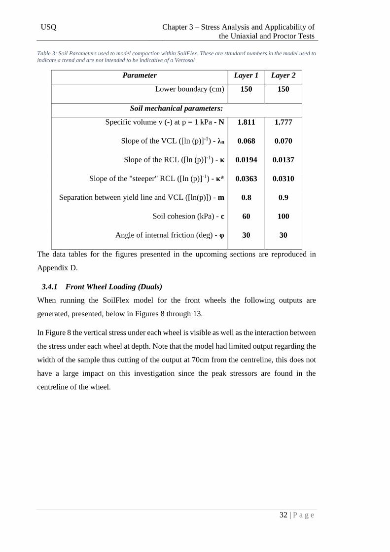
USQ Chapter 3 – Stress Analysis and Applicability of
the Uniaxial and Proctor Tests
32 | P a g e
Table 3: Soil Parameters used to model compaction within SoilFlex. These are standard numbers in the model used to
indicate a trend and are not intended to be indicative of a Vertosol
Parameter Layer 1 Layer 2
Lower boundary (cm) 150 150
Soil mechanical parameters:
Specific volume v (-) at p = 1 kPa - N 1.811 1.777
Slope of the VCL ([ln (p)]-1) - λn 0.068 0.070
Slope of the RCL ([ln (p)]-1) - κ 0.0194 0.0137
Slope of the "steeper" RCL ([ln (p)]-1) - κ* 0.0363 0.0310
Separation between yield line and VCL ([ln(p)]) - m 0.8 0.9
Soil cohesion (kPa) - c 60 100
Angle of internal friction (deg) - φ 30 30
The data tables for the figures presented in the upcoming sections are reproduced in
Appendix D.
3.4.1 Front Wheel Loading (Duals)
When running the SoilFlex model for the front wheels the following outputs are
generated, presented, below in Figures 8 through 13.
In Figure 8 the vertical stress under each wheel is visible as well as the interaction between
the stress under each wheel at depth. Note that the model had limited output regarding the
width of the sample thus cutting of the output at 70cm from the centreline, this does not
have a large impact on this investigation since the peak stressors are found in the
centreline of the wheel.

USQ Chapter 3 – Stress Analysis and Applicability of
the Uniaxial and Proctor Tests
33 | P a g e
Figure 8: SoilFlex output representing vertical stress distribution under the front wheels of a JD7760. Note that the
output has been cut off at 70 cm from the centreline, this has no effect on the use of the results as the peak stresses are
under the centreline of the wheel
In Figure 9, below, it is shown that the peak surface loading is generated at the centre of
the wheel, the value of this loading is 375 kPa and this value decreases radially from the
centre.
Figure 9: SoilFlex output representing the vertical contact stress as a result of the JD7760’s front wheels
0.0
42.5
87.5
132.5
-
70
-
60
-
50
-
40
-
30
-
20
-
10
010203040506070
Dep
th (
cm)
Distance (perpendicular to driving direction) from the centre
(cm)
Vertical stress σz (kPa)
360-380
340-360
320-340
300-320
280-300
260-280
240-260
220-240
200-220
180-200
160-180
140-160
120-140
100-120
80-100
60-80
40-60
20-40
0-20
10
-13
-360
50
100
150
200
250
300
350
400
-38 -28 -18 -8 2 12 22 32 42
Y(c
m)
Ver
tica
l S
tres
s (k
Pa)
X (cm)
Vertical Stress
350-400
300-350
250-300
200-250
150-200
100-150
50-100
0-50
Driving

USQ Chapter 3 – Stress Analysis and Applicability of
the Uniaxial and Proctor Tests
34 | P a g e
In Figure 10, below, the vertical stress over the considered depth (1.5m) is shown in the
centreline of the wheel path. This location is equidistant from either wheel. This output
shows an increase in stress at a depth of 65 cm, producing a peak of 52 kPa. This suggests
that the stresses of each wheel only interact at the aforementioned depth, confirmed in
Figure 9, above, and although this is a small stress it could be considered to have some
impact on bulk density. This means that the surface between the wheels experiences
minimal stress according to SoilFlex, although in-field measurement documented by
Bennett et al. (2015) suggests that a compaction pan, similar to a plough pan, can be seen
to develop between dual wheel configurations at a depth of 20–40 cm.
Figure 10: SoilFlex output under the centre line of the sample showing the distribution of stress with depth as a result
of traffic by the front wheels of the JD7760. Note that the centreline of the sample is equidistant from either wheel
The result of this stress distribution is depicted in Figure 11. This has assumed an initial
bulk density of 1.67 g/cm3. In Figure 10 it can be seen that the peak bulk density (in
between the two wheels) is at a depth that is lower than the peak stress. The bulk density
increase is very small. This suggests that the 52 kPa peak is only just sufficient to cause
compaction.
0
50
100
150
0 10 20 30 40 50 60
Dep
th (
cm)
Vertical stress (kPa) Centre Line)
1st wheel

USQ Chapter 3 – Stress Analysis and Applicability of
the Uniaxial and Proctor Tests
35 | P a g e
Figure 11: SoilFlex output under the centre line of the sample showing the change in bulk density with depth. Note that
the centreline of the sample is equidistant from either wheel. The green line represents the initial bulk density whilst
the blue lien represents the bulk density after one pass of the wheel
The vertical stress under the wheel is shown in Figure 12, below, (each wheel produces
an identical distribution). In Figure 12 shows an exponential decrease in the vertical stress
from the peak loading at the surface. This results in the stress being negligible after a
depth of 1m where the stress has been reduced to 40 kPa.
Figure 12: SoilFlex output showing the distribution of vertical stresses under one of the front wheels
0.00
50.00
100.00
150.00
1.6599 1.6600 1.6601 1.6602D
epth
(cm
)
Bulk density (g cm-3) under the centre line (between both wheels)
Initial bulk
density
After first
wheel
0
50
100
150
0 50 100 150 200 250 300 350 400
Dep
th (
cm)
Vertical stress (kPa) - Under Wheel
1st wheel

USQ Chapter 3 – Stress Analysis and Applicability of
the Uniaxial and Proctor Tests
36 | P a g e
Supporting the findings shown above, Figure 13, below, shows that, as the stress falls
below approximately 50-60 kPa the increase in bulk density falls to zero.
Figure 13: SoilFlex output showing the change in bulk density under one of the front wheels. The green line represents
the initial bulk density whilst the blue line represents compaction after trafficking
3.4.2 Rear Wheel Loading
Similar to the front wheels when running the SoilFlex model for the outputs for the rear
wheel are presented below.
Figure 14, below, shows the vertical stress distribution under the rear wheel, with a peak
of approximately 570 kPa under the centre of the wheel.
0
50
100
150
1.67 1.67 1.68 1.68 1.69 1.69 1.70 1.70 1.71 1.71
Dep
th (
cm)
Bulk density (g cm-3) under the centre line of the wheel track
Initial bulk density
After first wheel

USQ Chapter 3 – Stress Analysis and Applicability of
the Uniaxial and Proctor Tests
37 | P a g e
Figure 14: SoilFlex output representing vertical stress distribution under the rear wheel of a JD7760.
The contact stress provided by the tyre is shown in Figure 15. Again the stress peaks in
the centre and decreases radially outward, however in this case the peak contact stress of
570 kPa.
Figure 15: SoilFlex output representing the vertical contact stress as a result of the JD7760’s rear wheel
0.0
37.5
77.5
117.5
-
50
-
40
-
30
-
20
-
10
01020304050
Dep
th (
cm)
Distance (perpendicular to driving direction) from the centre
(cm)
Vertical stress σz (kPa)
560-580540-560520-540500-520480-500460-480440-460420-440400-420380-400
50
274
-19-42
0
100
200
300
400
500
600
-50-40-30-20-10 0 10 20 30 40 50 Y (
cm)
Str
ess
(kP
a)
X (cm)
Vertical Stress
500-600
400-500
300-400
200-300
100-200
0-100
Driving

USQ Chapter 3 – Stress Analysis and Applicability of
the Uniaxial and Proctor Tests
38 | P a g e
The vertical stress distribution follows a similar trend to the front wheels (Figure 16)
however with a higher starting value. The change in bulk density is shown, below, in
Figure 17, where it can again be seen that the change in bulk density falls to zero when
the stress falls to a value less than approximately 50 kPa.
Figure 16: SoilFlex output under the centre line of the sample showing the distribution of stress with depth as a result
of trafficking by the rear wheel of a JD7760
Figure 17: SoilFlex output showing the change in bulk density with depth as a result of trafficking by the rear wheel of
a JD7760. The green line represents initial bulk density whilst the blue line represents to bulk density after a single
pass
0
50
100
150
0 100 200 300 400 500 600
Dep
th (
cm)
Vertical stress (kPa)
1st wheel
0.00
50.00
100.00
150.00
1.65 1.66 1.67 1.68 1.69 1.70 1.71 1.72 1.73 1.74
Dep
th (
cm)
Bulk density (g cm-3) under the centre line of the wheel track
Initial bulk densityAfter first wheel

USQ Chapter 3 – Stress Analysis and Applicability of
the Uniaxial and Proctor Tests
39 | P a g e
3.5 SoilFlex Analysis and Comparison
From the model outputs a number of conclusions can be drawn in relation to the loading
and its nature. These conclusions will allow informed selection of loadings to test when
replicating the loading of the JD7760.
In order to analyse the front wheel loading of the JD7760 two key aspects of the outputs
should be considered: the influence of a single wheel and the effect of the two wheels
interacting.
As seen in Figures 8 and 9 the peak contact stress of the wheels is generated from a single
wheel, in isolation of the effects of the other wheel. This is very obvious in Figure 9 where
the green “unchanged” bulk density is shown between each wheel. As the depth increases
the stress generated by the wheels begin to interact elongating the area of stress influence.
This is supported in Figures 10 and 12 where the stress under one wheel can be compared
to the stress under the centreline of the trafficked area (i.e. centred between the wheels).
This comparison shows that the wheels do interact although the interaction is negligible
when compared to the peak loadings generated under the single wheel. Thus the loadings
underneath the centre of the wheel will be considered for comparison between the front
and rear wheels.
Upon comparison between the front and rear wheel loading cases similarities are
immediately visible: the nature of the decrease of stress in exponential with the bulk
density influenced by the wheel compaction up to a depth of approximately 70-90 cm,
despite the differences in additional loading. Suggesting that considering data to a depth
of 1m is a conservative approach. In addition to this the peak loadings of both the front
and rear wheels occurs under the centre of the tyre.
In addition to this the change in vertical stress is considerably lower after depth of 1m
when compared to the change from 0-1m. Using this as a boundary it is now possible to
compare the raw data with the aim of identifying a range of applicable stresses for testing.
This has been achieved through the use of Table 4 below.

USQ Chapter 3 – Stress Analysis and Applicability of
the Uniaxial and Proctor Tests
40 | P a g e
Table 4: Tabulated SoilFlex output listing the stresses experienced at each depth and the average stresses over a range
of depth with an aim to simplify the selection of applicable loads to test
Rear Front
Depth
(cm)
Bulk
Density
(g/cm3)
Vertical
Stress
(kPa)
Average
Vertical
Stress
(kPa)
Bulk
Density
(g/cm3)
Vertical
Stress
(kPa)
Average
Vertical
Stress
(kPa)
0.00 570 570 375 375
2.50 1.73 564
556
1.71 371
365.67 7.50 1.73 564 1.71 371
12.50 1.72 539 1.70 355
17.50 1.71 494
437
1.70 325
287.67 22.50 1.70 438 1.69 288
27.50 1.69 380 1.69 250
32.50 1.69 326
281
1.69 215
185.67 37.50 1.68 279 1.68 184
42.50 1.68 239 1.68 158
47.50 1.68 206
180
1.68 137
120.00 52.50 1.68 178 1.68 119
57.50 1.67 155 1.67 104
62.50 1.67 136
121
1.67 92
82.33 67.50 1.67 120 1.67 82
72.50 1.67 106 1.67 73
77.50 1.66 95
86
1.67 66
60.33 82.50 1.66 85 1.67 60
87.50 1.66 77 1.67 55
92.50 1.66 69
63
1.67 50
46.67 97.50 1.66 63 1.67 47
102.50 1.66 57 1.67 43
From Table 4 it can be seen that despite different loadings the change in bulk density is
similar at 27.5 cm depth. Additionally the rear wheel is shown to have a larger influence

USQ Chapter 3 – Stress Analysis and Applicability of
the Uniaxial and Proctor Tests
41 | P a g e
on the compaction at a depth, in spite of a lower contact stress. This notion is supported
in the literature.
This model suggests that the stress values less than 100 kPa do not have a noticeable
impact on soil compaction, suggesting that it would provide a good lower bound to the
considered stresses.
The peak loading that is generated by the harvester is approximately 600 kPa under the
rear wheel and, in both cases, decreases logarithmically with depth. This loading pattern
is used to plausibly suggest that testing loads of 600, 400, 200 and 100 kPa will generate
a bulk density that will give results that are indicative of compaction that has been
experienced in the field. This is because the loads are representative of the stresses that
are experienced over the applicable depth of soil. However as has been described in the
literature review, similar testing has been undertaken by Suzuki et al. (2013) finding that
the stresses of 800 kPa and 1600 kPa were of good use for an indicative test, thus these
loadings will also be considered to provide direct comparison to their work.
3.6 Critical Analysis and Modification of Assessment Methods
As previously stated; the literature suggests that the most common methods of
determining the reference bulk density are the Uniaxial and the Proctor Tests. Both of
these tests use a standard compactive force to produce a compaction. For this dissertation
both the standard tests and variations to these tests will be analysed.
3.6.1 Standard Uniaxial Test
The standard Uniaxial Test most referenced in the literature has been described by
Häkansson (1990). In selecting the Uniaxial Compression Test as the preferred method
for reference testing Häkansson considered a variety of factors that would best describe
the conditions experienced in the field. In addition to this a preference was stated for
testing that could be easily reproduced without a large expenditure of man hours. This
reasoning and its applicability are investigated below.
The chief conditions that were examined by Häkansson included the size and inclusions
of foreign matter in the samples, the moisture content and the manner and intensity of
loading (Håkansson 1990). Furthermore this suggests that, whilst the exact size of the
specimen is not critical, it should be as large as possible and include the same stones,
plant residues etc. that is included in the field; easily achieved in bulk sampling.

USQ Chapter 3 – Stress Analysis and Applicability of
the Uniaxial and Proctor Tests
42 | P a g e
Perhaps the most important key parameter that Häkansson considered in his experimental
design is the mode and intensity of the loading stating that the “reference test should have
a mode and intensity of loading similar to that in the applications concerned” (Håkansson
1990). Suggested that the loading of agricultural soils is generally of the static type and
is supported in the literature review (Chapter 2). As such this dissertation utilised a static
loading in the Uniaxial Compression Test.
The chosen loading intensity (200 kPa) was selected by Häkansson due to its location in
the upper range of the loading the soil experiences, at the time of method development
(prior to the 1990s). This lends strong merit to the necessity of increasing the reference
loading considering the current loading of more modern machinery. A load in the higher
regions of what is experienced by the soil was selected to avoid the soil being pre-
compressed by a load greater than the testing load. It is also stated that the load should
not be so high as to detract from the relevance of the test.
The moisture content in Häkansson’s tests was managed through the use of an
exceptionally long loading time and a porous base, allowing for equalisation of the
moisture content of the samples. This process took one week (Håkansson 1990).
3.6.2 Modifications to the Uniaxial Test
In order to suit the requirements and time limitations of this dissertations some changes
to the methodology of the standard Uniaxial Test presented by Häkansson (1990) are
required. The modifications will either reduce the time of testing, match the available
materials for testing or to include variable loading.
The introduction of variable loading will follow the methods presented by Suzuki et al.
(2013). Not all of the method presented by Suzuki et al. will be applicable since the paper
considers no tillage plots however the methods of alteration considered are still
applicable.
The first alteration to the Uniaxial Test presented by Häkansson (1990) is a change to the
applied loading; as described in Suzuki et al. (2013). This is achieved by altering the load
applied to the sample and comparing the resultant bulk density to values gathered in the
field (and generated within the SoilFlex model). Differing from Suzuki et al., the actual
values of loading will be altered to suit the values produced in SoilFlex: 100, 200, 400,
600, 800 and 1600 kPa. These values should give an indication of the soil over its depth

USQ Chapter 3 – Stress Analysis and Applicability of
the Uniaxial and Proctor Tests
43 | P a g e
and the utilisation of the higher stresses may be used to allow for future growth as may
be necessary.
Further alteration to the test will is required to combat major hindrances to the timeline.
This includes consideration of the moisture content and time of loading (noting these are
somewhat interrelated). Häkansson’s (1990) original method utilises a drained test to
equalise the moisture content between samples, however this requires approximately one
week per test. As such a different method of accounting for water content is required.
This can be achieved in two ways: test a range of moisture contents as per the Proctor
Test or test a single moisture content taken as a standard.
Ideally a range of moisture contents would be used as a means for calculating the
maximum bulk density under each load. This, however, would require significantly more
testing than required by a standard moisture content. The main drawback in using a
standard moisture content is the variability between soils. For example, the moisture
content that produces maximum compaction in one soil may produce significantly more
or less compaction in another. However this could be negated since the compaction
recorded will be used as an arbitrary reference to the soil itself and would only be an issue
if the compaction generated was lower than that experienced in the field.
It is suggested that using a range of moisture contents to produce a maximum compaction
would be most applicable to determine the reference compaction. This however will
dramatically increase the time required for testing. A way around this issue within this
project could be to conduct the Proctor Test before the Uniaxial Compression Testing.
This will allow accurate determination of the ideal moisture content for compaction for
use within the Uniaxial Testing. This moisture content will be the same between tests.
Since the moisture content is no longer a factor it is possible to reduce the time of loading
to a more reasonable level. Since most of the compaction occurs during the first pass of
a vehicle in the field relatively low loading times can be used. Suzuki et al. (2013) has
used 5 minutes, which represents the current experimental process also.
3.6.3 Standard Proctor Test
The Proctor Test uses a number of sub-replicates of the same soil sample and volume
compacted at a constant load with moisture varying for each sub-replicate. This allows
the optimum moisture content for soil compaction to be determined for the given load. At
the optimum moisture content, the maximum dry density occurs for that same given load,

USQ Chapter 3 – Stress Analysis and Applicability of
the Uniaxial and Proctor Tests
44 | P a g e
which is then used to provide the reference density for the given load. Testing refers to
AS1289.5.1.1.
3.6.4 Modifications to the Proctor Test
Given the availability of the Proctor Test equipment it is postulated that the simplest
manner in which to alter the loading generated in the test is through altering the number
of blows to each layer. Two hammer types are available: the standard and modified
hammer. The standard hammer has been used in this situation to provide a higher
resolution in the number of blows provided to each layer for the smaller stresses, allowing
more uniform compaction (i.e. more blows are required to reach a stress value, thus when
considering lower values the hammer is more likely to compact the entire surface of the
soil sample) and closer adherence to the required loads.
The compactive effect of the Proctor blows on the soil sample can be calculated following
the equations stated by Raghaven and Ohu (1985) (Equations 3.7, 3.8):
𝐶𝑜𝑚𝑝𝑎𝑐𝑡𝑖𝑣𝑒 𝐸𝑓𝑓𝑜𝑟𝑡 (𝐶) =𝑀 ∗ 𝑔 ∗ ℎ ∗ 𝐿 ∗ 𝑁𝐵
𝑉
Eqn 3.7
Where:
𝑀 = 𝑚𝑎𝑠𝑠 𝑜𝑓 𝑡ℎ𝑒 ℎ𝑎𝑚𝑚𝑒𝑟 (𝑘𝑔)
𝑔 = 𝑎𝑐𝑐𝑒𝑙𝑒𝑟𝑎𝑡𝑖𝑜𝑛 𝑑𝑢𝑒 𝑡𝑜 𝑔𝑟𝑎𝑣𝑖𝑡𝑦 (𝑚
𝑠2)
L = number of layers
ℎ = ℎ𝑒𝑖𝑔ℎ𝑡 𝑜𝑓 𝑓𝑎𝑙𝑙 (𝑚)
𝑁𝐵 = 𝑁𝑢𝑚𝑏𝑒𝑟 𝑜𝑓 𝑏𝑙𝑜𝑤𝑠 𝑝𝑒𝑟 𝑙𝑎𝑦𝑒𝑟
𝑉 = 𝑉𝑜𝑙𝑢𝑚𝑒 𝑜𝑓 𝑠𝑎𝑚𝑝𝑙𝑒 (𝑚3)
Using the standard conditions described in AS1289.5.1.1 a compactive effort is produced:
𝐶 =2.7 × 9.81 × 0.3 × 3 × 25
0.001
𝐶 = 595.95 𝑘𝑃𝑎
This matches the compactive effort stated in AS1289.5.1.1 of 596 kPa, thus the equation
is assumed to be reasonable.
Furthermore Raghavan and Ohu (1985) suggest an equation to link static loading with the
Proctor loading, (R2 value= 0.998 @ 0.0001). This relationship is critical as it allows the

USQ Chapter 3 – Stress Analysis and Applicability of
the Uniaxial and Proctor Tests
45 | P a g e
comparison of the impact load of the Proctor Test to be expressed in terms of a static load.
The differences in these loading types have been discussed in the literature review.
𝑆𝑡𝑎𝑡𝑝 = 66.70 + 22.10𝑃𝑟𝑜𝑐𝐵 Eqn 3.8
Where:
𝑆𝑡𝑎𝑡𝑝 = 𝑠𝑡𝑎𝑡𝑖𝑐 𝑝𝑟𝑒𝑠𝑠𝑢𝑟𝑒 𝑒𝑞𝑢𝑖𝑣𝑎𝑙𝑒𝑛𝑐𝑒
𝑃𝑟𝑜𝑐𝐵 = 𝑁𝑢𝑚𝑏𝑒𝑟 𝑜𝑓 𝑃𝑟𝑜𝑐𝑡𝑜𝑟 𝐵𝑙𝑜𝑤𝑠
This relationship is true for the standard Proctor Test.
This set of equations has been graphed in Figure 18 to provide a visual indication of the
relationships with the data tables included in Appendix E for reference.
Figure 18: Standard Proctor Test static load equivalence showing a linear increase in equivalent static load provided
by a number of compactive blows provided by the standard Proctor Test
As can be seen, the equivalent static load is typically greater than the actual compactive
effort although as the number of blows increases the difference in actual and equivalent
loading decreases. This indicates that the sharp impact of the hammer fall has a greater
effect than a static load, which is discussed within the literature review (Chapter 2).
The above relationship has been used to generate the required number of blows,
presented, below, in Table 5. This table also displays the actual equivalent static pressure.
As previously discussed, in order for the Proctor Test to be reliable some degree of
uniform compaction must be applied to the soil, as the Proctor Test uses a soil column of

USQ Chapter 3 – Stress Analysis and Applicability of
the Uniaxial and Proctor Tests
46 | P a g e
greater diameter than the diameter of the hammer. Hence, multiple blows represent
multiple impacts as might occur in the passing of a sheep’s foot roller. Thusly, the static
loading requirement of 100 kPa has been eliminated from assessment with the Proctor
Test variant as one blow is not sufficient for uniform compaction.
Table 5: Standard Proctor Test static load equivalence at the required loadings for testing
Static Load
Required (kPa)
Number of Proctor
Blows
Equivalent
Static Load
(kPa)
100 1 (not to be included) 88.8
200 6 199.3
400 15 398.2
600 24 (use standard of 25) 597.1
800 33 796.0
1600 69 1591.6
These loadings will occur at the optimum moisture content provided by the unmodified
Proctor Tests.
3.6.5 Experimental Factor Summary
In summary, based on the critical analysis of methods and modification of these, the
experimental factors for this study are identified as:
1. The Uniaxial Compression Test modified to suit a single pass of a heavy machine
with the loads 200, 400, 600, 800 and 1600 kPa
2. The Proctor Test conducted as per the standard and modified variants of the test
to suit a range of static load synonymous with large machinery and literature
thresholds using 6, 15, 25, 33 and 69 blows (representing static loadings of 200,
400, 600, 800 and 1600 kPa)
The bulk density gathered from these tests will be compared to those gathered in the field
as part of an interrelated project.

USQ Chapter 4 - Experimental Procedure
47 | P a g e
Chapter 4 - Experimental Procedure
Given the stress analysis conducted for the JD7760 using SoilFlex, and the ensuing
methodological analysis and modification (Chapter 3), the detailed experimental
procedure is set out below for each test:
4.1 Soil Sampling and Preparation
This project has utilised bulk disturbed samples collected from a variety of locations listed
in Table 6. These samples have then been assigned an alphabetic handle to simplify
discussion.
Table 6: Sample Locations and Handle
Location Handle
Toobeah, QLD A
Goondiwindi, QLD B
Yelarbon, QLD C
Aubigny, QLD D
Jimbour, QLD E
Warren, NSW F
Sampling was conducted over a depth of 0-20 cm below the surface using handheld
shovels. The samples were then placed in containers and protected from drying.
Once the samples were collected the soil was dried in an oven at 105°C for 4-7 hours to
allow soil to be dry enough for subsequent handling without smearing of soil structure
prior to the experiment. Following this the sample was carefully made to pass through a
19mm sieve by breaking down the larger peds. The soil was then allowed to air dry.
A smaller air-dried sub-sample was placed in the oven at 105°C for 72hrs to determine
the oven dry moisture content allowing the calculation of true moisture content during
the tests.
4.2 Standard Proctor Test
The Proctor Tests were conducted with reference to AS1289.5.1.1.

USQ Chapter 4 - Experimental Procedure
48 | P a g e
4.2.1 Equipment
The equipment used was as follows:
1. Standard Proctor mould A: Ø D=105mm, H=115mm with a baseplate and collar
that can be firmly attached
2. 2.7kg steel rammer/hammer
3. Level rigid foundation for testing
4. Scales (±0.005kg)
5. Strong spatula
6. Steel straightedge
7. Mixing apparatus
8. Shovel
9. Sealable containers
10. Screw driver (for removing sample from mould and for attaching the mould to the
base plate)
Photos of the equipment are available in Appendix F. AS1289.5.1.1 shows schematics
and tolerances for the mould and hammer.
4.2.2 Procedure
The testing procedure was as follows (AS1289.5.1.1):
1. Soil samples were prepared according to the procedure in Section 4.1
2. Soil was moistened to a gravimetric moisture content that was approximated to be
lower than the optimum moisture content and was allowed to cure for 20-30min
3. Soil was placed in the Proctor mould such that it was filled approximately 50%
4. The Proctor hammer was then used to compact the soil over 25 blows. These
blows were spaced evenly over the surface
5. An approximately equivalent volume of soil was again added to the mould to
create the second lift
6. The Proctor hammer was then used to compact the soil over 25 blows. These
blows were spaced evenly over the surface
7. An approximately equivalent volume of soil was again added to the mould to
create the third lift
8. The Proctor hammer was then used to compact the soil over 25 blows. These
blows were spaced evenly over the surface

USQ Chapter 4 - Experimental Procedure
49 | P a g e
9. The collar was then removed and the soil surface trimmed such that it was level
with the edge of the collar
10. The mass of the mould and the soil was then taken and used to calculate the wet
as in Equation 4.1 below:
𝜌𝑤𝑒𝑡 =𝑀𝑎𝑠𝑠
𝑉𝑜𝑙𝑢𝑚𝑒
Eqn 4.1
Where:
𝑀𝑎𝑠𝑠 = 𝑚𝑎𝑠𝑠 𝑜𝑓 𝑚𝑜𝑢𝑙𝑑 𝑎𝑛𝑑 𝑠𝑜𝑖𝑙 − 𝑚𝑎𝑠𝑠 𝑜𝑓 𝑡ℎ𝑒 𝑚𝑜𝑢𝑙𝑑
11. The dry bulk density was then calculated accounting for the moisture content
12. The soil was then removed from the mould and the equipment was cleaned
13. Steps 2 through 11 are then repeated for moisture contents such that the optimum
moisture content has been adequately straddled i.e. two points either side of the
optimum moisture content were found
14. The removed soil was re-prepared as per chapter 4.1 for use in later tests
4.3 Standard Proctor Test with Modified Load
The modified loading of the Proctor Test was achieved by altering the number of blows
per layer as discussed in Chapter 3, otherwise the procedure was as per AS1289.5.1.1.
4.3.1 Equipment
The equipment used was as per that in Sub-section 4.2.1.
4.3.2 Procedure
The testing procedure was again in accordance with AS1289.5.1.1 and as per Sub-section
4.2.2. However, where 25 blows were used, the number of blows was changed to match
the static loads as detailed in Table 5. The test was repeated three times for each level of
compactive effort (Static load equivalent).
4.4 Uniaxial Test
The procedure developed for the Uniaxial Test was determined as per Häkansson (1990)
but was modified procedurally to suit a single pass of heavy machinery and to provide
comparison to Suzuki et al. (2013).
4.4.1 Equipment
The equipment used during this testing is included below:

USQ Chapter 4 - Experimental Procedure
50 | P a g e
1. Standard Proctor mould B: Ø D=152mm, H=132.5mm with a baseplate and collar
that can be firmly attached
2. Shop press – rated to 6,000kg
3. Load cell calibrated and rated to 10,000kg
4. Level rigid foundation for testing
5. Scales (±0.005kg)
6. Strong spatula
7. Steel straightedge
8. Ruler
9. Mixing apparatus
10. Shovel
11. Sealable containers
12. Screw driver (for removing sample from mould and for attaching the base plate to
the mould)
4.4.2 Procedure
1. Soil samples were prepared according to the procedure in Section 4.1.
2. Soil was moistened to the optimum gravimetric moisture content that was
determined in 4.2.2 and was allowed to cure for 20-30 minutes
3. Soil was added to the mould
4. A load plate was placed on the soil (assuming that the mass of the load plate has
negligible effects of the compaction of the soil)
5. The mould and soil were placed in the shop press and the load cell was placed on
top of the load plate
6. A load of 200 kPa was applied using the shop press for five minutes (some
adjustment was required during the first minute of loading to ensure the correct
load was maintained.
7. The deformation of the sample was then measured at four points on the surface of
the sample and the average was taken (unless there was significant variation in
the height)
8. The average deformation was then used to calculate the volume of the soil
9. The soil and mould was then weighed and used to calculate the dry and weight
bulk densities as per steps 10 and 11 in Section 4.2.2.
10. The soil was then removed from the mould and the equipment was cleaned

USQ Chapter 4 - Experimental Procedure
51 | P a g e
11. Steps 2 through 11 were then repeated using the following loads: 400, 600, 800
and 1600 kPa as determined in chapter 3. The test was repeated three times for
each compactive effort
12. The soil was then re-prepared as per 4.1
4.5 Safety
Safety was paramount in conducting the experimentation. A full copy of the USQ safety
forms are included in Appendix G however the key points and safety features will be
briefly discussed here.
4.5.1 General
The general safety issues that were encountered in the process of experimentation mainly
pertained to air quality and physical safety issues.
Since the soils were moved in a dried condition any pouring or violent disruption to the
soil resulted in clouds of dust particles that could possibly cause harm if inhaled. This
was mitigated by ensuring that the work space was open and well ventilated, allowing
cross breezes to disperse the particles quickly. When this was not possible the task was
undertaken outdoors or with the operator wearing a dust mask.
The physical safety issues that were presented in the testing related to the movement and
lifting of the heavy containers of soil and the repetitive movements required when
performing the Proctor Test, particularly in the cases where >25 blows were required.
Mitigation of these issues was in the form of previously received training and the use of
correct technique.
4.5.2 Proctor Tests
In the Proctor Test the main hazard that was presented relates to the use of a falling
hammer. This constituted a minor pinching/crushing hazard to the operator. The
operator’s familiarity with the hammer and its correct operation mitigated the risk to an
acceptable level. To operate the hammer as intended the user only interacts with the non-
moving parts.
4.5.3 Uniaxial Tests
The Uniaxial Test presents a greater risk than the Proctor Test however the hazards are
not likely to occur in such a small number of uses. This was because the hazards
associated with using the equipment relate to its catastrophic failure which was unlikely
to occur given that anticipated loadings were well below the safe operating limits.

USQ Chapter 4 - Experimental Procedure
52 | P a g e
If failure were to occur the operator was separated from the equipment by a physical
barrier which all but completely alleviates the hazard from the user.

USQ Chapter 5 – Results
53 | P a g e
Chapter 5 – Results
5.1 Introduction
This section presents the major results with in-depth and integrated explanation occurring
in Chapter 6 (Discussion). Results are presented on the basis of the individual
measurements. This chapter will also present the in situ bulk density data taken in-field
allowing comparisons of the laboratory results to in-field observed results from a load
directly applied by a JDD7760 cotton picker. The raw data from the below tests has been
included in Appendices H and I.
5.2 Proctor Test
The presentation of the results from the proctor tests will be undertaken in two parts, one
investigating the standard compactive effort at multiple moisture contents as described in
Section 4.2, the other describing the modified compactive efforts at an un-changing
moisture content (Section 4.3).
5.2.1 Standard Compactive Effort
In undertaking the testing described in Section 4.2 the following results have been
generated (Figures 19 to 23). In the generation of these results an optimum moisture
content (OMC) has been selected to allow the progression of testing (manipulation to
static load applicable to likely imposed agricultural traffic loading).
Sample A
The proctor testing of Sample A experienced difficulties that resulted in inconclusive
results that could not be used to generate the OMC. Whilst the data presented in Table
and Figure 19 below appears to show a parabolic trend the data gathered is not seen to be
representative of the soil. This is because the apparatus was not able to function as
intended; with each strike significant volume of sample was removed as clay stuck to the
hammer. This prevented the un-obstructed fall of the hammer, reducing the energy input
into the soil voiding the results shown below.

USQ Chapter 5 – Results
54 | P a g e
Figure 19: Proctor graph showing the change in bulk density with moisture content, note the values are seen to be an
inaccurate representation of the soils behaviour
Sample B
Sample B followed the expected trend. Four moisture contents were tested as per
AS1289.5.1.1 and were deemed to adequately straddle the optimum moisture content.
This is shown below in Figure 20.
Figure 20: Proctor graph for Sample B showing a parabolic nature with an optimum moisture content of 17% and a
corresponding peak bulk density of 1.56 g/cm3
1.35
1.4
1.45
1.5
1.55
1.6
0.00% 5.00% 10.00% 15.00% 20.00% 25.00% 30.00%
Dry
Bu
lk D
ensi
ty (
g/cm
3)
Moisture Content (%)
Sample A - Standard Proctor Test
y = -56.368x2 + 19.103x - 0.0545R² = 0.958
1.1
1.2
1.3
1.4
1.5
1.6
1.7
0.00% 5.00% 10.00% 15.00% 20.00% 25.00% 30.00%
Dry
Bu
lk D
ensi
ty (
g/cm
3)
Moisture Content (%)
Sample B - Standard Proctor Test

USQ Chapter 5 – Results
55 | P a g e
A visual examination of Figure 20 shows that the optimum moisture content exists
between 15% and 20%, this however is insufficiently accurate for this project. As such a
trend line was overlaid on the data, supplying a strong relationship with the data
(R2=0.958). Through derivation and manipulation of this equation the optimum moisture
content can be given with confidence as 17%. The use of this equation can also allow the
determination of the peak density that could be achieved at the optimum moisture content.
This gives the peak bulk density of 1.56 g/cm3.
Sample C
Testing on Sample C occurred largely without issue, however after testing four moisture
contents a peak was not straddled. This resulted in the testing of a greater number of
moisture contents as shown in Appendix H. As a result of this, the testing of a higher
number of moisture contents gives an understanding of the increase of the moisture
content over a wider range. The data resulting from the test is presented below in Figure
21.
Figure 21 Proctor graph for Sample C showing a parabolic nature with an optimum moisture content of 16% and a
corresponding peak bulk density of 1.5 g/cm3
As can be seen the data generally follows a parabolic curve, described by a quadratic
equation with an R2 value of 0.9051 representing a good fit. Despite the data generally
following the trend, one point at approximately 18% moisture content is lower than
expected. Using the same calculative process as described for Sample B the optimum
y = -30.103x2 + 9.56x + 0.7367R² = 0.9051
1.25
1.3
1.35
1.4
1.45
1.5
1.55
0.00% 5.00% 10.00% 15.00% 20.00% 25.00% 30.00%
Dry
Bu
lk D
ensi
ty (
g/cm
3)
Moisture Content (%)
Sample C- Standard Proctor Test

USQ Chapter 5 – Results
56 | P a g e
moisture content was found to be 16% and the peak bulk density was found to be
approximately 1.5 g/cm3.
Sample D
Again, during testing for Sample D the optimum moisture content was not identified after
4 iterations, as such, a greater number of tests were undertaken. This has resulted in data
that follows a quadratic trend with an extremely strong R2 value of 0.9993. The optimum
moisture content was derived as 28.1% with a corresponding peak bulk density of 1.21
g/cm3 is produced, shown below in Figure 22.
Figure 22 Proctor graph for Sample D showing a parabolic nature with an optimum moisture content of 28.1% and a
corresponding peak bulk density of 1.21 g/cm3
Sample E
Sample E suggests that the maxima has just been exceeded by the first moisture content
tested, although fitting a trend line to this moves the OMC to a lower moisture content.
Whilst, the quadratic equation fitted has an R2 value of 0.9783 indicating a good fit, the
OMC value for this soil should have lower confidence placed in it than for previous
successful proctor tests. However, for the sake of comparing modified compression
methods, the relative differences will still be applicable. For this sample the optimum
moisture content was found to be 22% generating a bulk density of 1.27 g/cm3, visualised
below in Figure 23.
y = -38.505x2 + 21.667x - 1.8339R² = 0.9993
1
1.05
1.1
1.15
1.2
1.25
0.00% 5.00% 10.00% 15.00% 20.00% 25.00% 30.00% 35.00% 40.00%
Dry
Bu
lk D
ensi
ty (
g/cm
3)
Moisture Content (%)
Sample D- Standard Proctor Test

USQ Chapter 5 – Results
57 | P a g e
Figure 23 Proctor graph for Sample E showing a parabolic nature with an optimum moisture content of 22% and a
corresponding peak bulk density of 1.27 g/cm3
Sample F
The proctor testing of Sample F experienced abnormalities that resulted in inconclusive
results. From Figure 24 the optimum moisture content might be assumed to be
approximately 20%, however, similar to Sample A, testing was not possible as the
apparatus no longer functioned as intended as, with each strike, a significant volume of
sample was remove with the hammer. This prevented the un-obstructed fall of the
hammer, reducing the energy input into the soil. This is shown below in Figure 24 where
the data is exceptionally erratic. Repeated iterations of the test resulted in similarly
inconclusive results across all moisture ranges. It is suggested that this soil may have
OMC of ~22%, demonstrated by a strongly correlated regression, but the inconclusive
nature of the results (highly variable even in repetition) suggest it would be unwise to
proceed with comparison at these values.
y = -15.446x2 + 6.8328x + 0.5157R² = 0.9783
1.05
1.1
1.15
1.2
1.25
1.3
0.00% 5.00% 10.00% 15.00% 20.00% 25.00% 30.00% 35.00%
Dry
Bu
lk D
ensi
ty (
g/cm
3)
Moisture Content (%)
Sample E- Standard Proctor Test
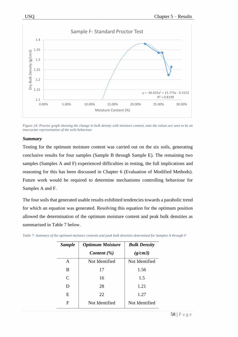
USQ Chapter 5 – Results
58 | P a g e
Figure 24: Proctor graph showing the change in bulk density with moisture content, note the values are seen to be an
inaccurate representation of the soils behaviour
Summary
Testing for the optimum moisture content was carried out on the six soils, generating
conclusive results for four samples (Sample B through Sample E). The remaining two
samples (Samples A and F) experienced difficulties in testing, the full implications and
reasoning for this has been discussed in Chapter 6 (Evaluation of Modified Methods).
Future work would be required to determine mechanisms controlling behaviour for
Samples A and F.
The four soils that generated usable results exhibited tendencies towards a parabolic trend
for which an equation was generated. Resolving this equation for the optimum position
allowed the determination of the optimum moisture content and peak bulk densities as
summarised in Table 7 below.
Table 7: Summary of the optimum moisture contents and peak bulk densities determined for Samples A through F
Sample Optimum Moisture
Content (%)
Bulk Density
(g/cm3)
A Not Identified Not Identified
B 17 1.56
C 16 1.5
D 28 1.21
E 22 1.27
F Not Identified Not Identified
y = -36.655x2 + 15.775x - 0.3152R² = 0.8199
1.1
1.15
1.2
1.25
1.3
1.35
1.4
0.00% 5.00% 10.00% 15.00% 20.00% 25.00% 30.00%
Dry
Bu
lk D
ensi
ty (
g/cm
3)
Moisture Content (%)
Sample F- Standard Proctor Test

USQ Chapter 5 – Results
59 | P a g e
5.2.2 Modified Compactive Effort
As discussed in Chapter 4 (Experimental Procedure) the use of the proctor test with a
modified compactive effort was carried out. Due to an undetected calculative error in
Microsoft EXCEL the moisture contents for some samples are higher than the optimum
values calculated in the initial proctor test. The implications of this will be discussed in
Chapter 6 (Evaluation of Modified Methods). Whilst tests were not carried out at the exact
OMC, the error was consistent between tests meaning that relative comparisons are valid
and thus useful in assessing the methodologies.
The modified proctor test resulted in data sets comparing an increasing compactive effort
(number of blows) with dry bulk density. This includes the bulk density values gathered
for 25 blows as per the standard test.
Generally speaking, the data tended to exhibit a logarithmic trend with the change in bulk
density becoming smaller as the compactive effort increases. This follows a steep increase
in the bulk density at the lower compaction levels.
For ease of reference, the equivalent static loading of the proctor test blows has been
presented in Table 8 for reference when considering the modified proctor test results. The
loading values in the below graphs (Figures 25 through 28) are listed in terms of number
of blows.
Table 8: Number of blows in the Proctor Test and equivalent static loads
Number
of Blows
Equivalent Static
Load (kPa)
6 200
15 400
25 600
33 800
69 16,000
Sample B
Shown in Appendix H is the data gathered in the proctor test with modified compactive
efforts when testing Sample B. This shows that generally the bulk density followed a
logarithmic trend approaching a plateau towards 69 blows. This is furthered below in
Figure 25 where the average bulk density at each compactive effort is shown. This figure

USQ Chapter 5 – Results
60 | P a g e
includes a trend line of logarithmic nature with an R2 value of 0.9234 representing a
reliable fit.
Figure 25: Proctor Test graph for Sample B showing a logarithmic relationship between the number of blows and bulk
density. Displayed points are the average of values presented in Appendix H
Sample C
The data gathered from sample C again shows a logarithmic trend, with the trend line
fitted to the average bulk densities showing an R2 value of 0.8817. This sample again
shows the bulk density having reduced change in bulk density between 33 and 69 blows
than between the earlier loading, visible in Figure 26.
Figure 26 Proctor Test graph for Sample C showing a logarithmic relationship between the number of blows and bulk
density. Displayed points are the average of values presented in Appendix H
y = 0.1308ln(x) + 1.1163R² = 0.9234
1.00
1.10
1.20
1.30
1.40
1.50
1.60
1.70
1.80
0 10 20 30 40 50 60 70 80
Dry
Bu
lk D
ensi
ty (
g/cm
3)
Number of Blows
Sample B - Proctor Test - Modified Compactive Effort
y = 0.1054ln(x) + 1.1459R² = 0.8817
1.00
1.10
1.20
1.30
1.40
1.50
1.60
1.70
0 10 20 30 40 50 60 70 80
Dry
Bu
lk D
ensi
ty (
g/cm
3)
Number of Blows
Sample C - Proctor Test - Modified Compactive Effort

USQ Chapter 5 – Results
61 | P a g e
Sample D
Sample D experienced the highest degree of variability of all the samples in this test,
showing a moderate R2 relationship of 0.467 when the average values are fitted to a
logarithmic trend. This is a better fit than provided before the exclusion of outliers. The
dataset is shown below in Figure 27. Given the clear trend displayed by other Samples
(B, C and E), the logarithmic trend is considered reliable, but further testing would be
required to confirm this.
Figure 27: Proctor Test graph for Sample C showing a logarithmic relationship between the number of blows and bulk
density. Displayed points are the average of values presented in Appendix H.
Sample E
Sample E exhibits the same logarithmic trend as shown for other samples with a reliable
fit provided by the trend line (R2=0.7785). This set of data, is shown below in Figure 28.
It is noted that whilst the trend line provides a strong relationship, the data suggests that
application of subsequent blows would result in very small bulk density increase, which
suggests an asymptote occurring. Hence, the trend line may be over predicting the impact
of future blows on soil density.
y = 0.0502ln(x) + 0.9524R² = 0.4677
0.90
0.95
1.00
1.05
1.10
1.15
1.20
0 10 20 30 40 50 60 70 80
Dry
Bu
lk D
ensi
ty (
g/cm
3)
Number of Blows
Sample D - Proctor Test - Modified Compactive Effort

USQ Chapter 5 – Results
62 | P a g e
Figure 28: Proctor Test graph for Sample E showing a logarithmic relationship between the number of blows and bulk
density. Displayed points are the average of values presented in Appendix H
Summary
Across all tested samples the increase in compactive effort has a logarithmic relationship
with the dry bulk density achieved, with most samples exhibiting an R2 value above 0.7
(Sample D shows a poorer fit with an R2 value of approximately 0.4). All samples
followed a trend that suggests a an asymptote density well before the specific gravity of
the particles, although it is important to note that if trend lines are extrapolated forward
that bulk density is allowed to exceed specific gravity, which is physically impossible.
Hence, boundary conditions must exist and this needs to be considered in interpreting the
results.
5.3 Uniaxial Compression Test
As described in Chapter 4 (Methodology), the uniaxial compression test was carried out
at a variety of loadings, equivalent to the loading the modified proctor test was carried
out at; allowing direct comparison between tests. Across all samples a logarithmic trend
was generally produced. This shows that an increase in the lower loadings resulting in a
large increase in bulk density relative to the gradient of the slope at higher loadings.
y = 0.0712ln(x) + 0.9386R² = 0.7785
1.00
1.05
1.10
1.15
1.20
1.25
1.30
0 10 20 30 40 50 60 70 80
Dry
Bu
lk D
ensi
ty (
g/cm
3)
Number of Blows
Sample E - Proctor Test - Modified Compactive Effort

USQ Chapter 5 – Results
63 | P a g e
Sample B
The data gained through the testing of Sample B has resulted in a reliable fit between the
average and the applied logarithmic trend, shown below in Figure 29. This has allowed
the data (Appendix I) to produce an R2 value of 0.9476.
Figure 29: Plot describing the logarithmic relationship between the increasing static load in the uniaxial compression
test and the bulk density of Sample B
Sample C
The trend of the averaged bulk densities shows a strong propensity towards a logarithmic
trend, displaying an R2 value of 0.9019, shown in Figure 30 below.
It is worth noting that the logarithmic trend fitted to this set of data shows the change in
bulk density at higher loadings producing a relatively high gradient.
Figure 30: Plot describing the logarithmic relationship between the increasing static load in the uniaxial compression
test and the bulk density of Sample C
y = 0.2303ln(x) - 0.2191R² = 0.9476
0.00
0.20
0.40
0.60
0.80
1.00
1.20
1.40
1.60
0.00 200.00 400.00 600.00 800.00 1000.00 1200.00 1400.00 1600.00 1800.00
Bu
lk D
ensi
ty (
g/cm
3)
Load (kPa)
Sample B - Uniaxial Compression Test
y = 0.0591ln(x) + 0.601R² = 0.9019
0.88
0.90
0.92
0.94
0.96
0.98
1.00
1.02
1.04
1.06
0.00 200.00 400.00 600.00 800.00 1000.00 1200.00 1400.00 1600.00 1800.00
Bu
lk D
ensi
ty (
g/cm
3)
Load (kPa)
Sample C - Uniaxial Compression Test

USQ Chapter 5 – Results
64 | P a g e
Sample D
The results from testing Sample D are shown in Appendix I. As previously mentioned the
fit applied is of logarithmic nature and in this case the trend is described by an R2 value
of 0.9964 which does suggests an extremely good fit. This can be seen in Figure 31.
Figure 31: Plot describing the logarithmic relationship between the increasing static load in the uniaxial compression
test and the bulk density of Sample D
Sample E
The data set gathered from uniaxial testing of Sample E shows greater variation, but still
provides a strong fit to the logarithmic trend within R2 value of 0.7226. The values
gathered in testing are shown in Figure 32.
Figure 32: Plot describing the logarithmic relationship between the increasing static load in the uniaxial compression
test and the bulk density of Sample E
y = 0.0921ln(x) + 0.1832R² = 0.9964
0.6
0.65
0.7
0.75
0.8
0.85
0.9
0.00 200.00 400.00 600.00 800.00 1000.00 1200.00 1400.00 1600.00 1800.00
Bu
lk D
ensi
ty (
g/cm
3)
Load (kPa)
Sample D - Uniaxial Compression Test
y = 0.0341ln(x) + 0.6093R² = 0.7226
0.70
0.72
0.74
0.76
0.78
0.80
0.82
0.84
0.86
0.88
0.00 200.00 400.00 600.00 800.00 1000.00 1200.00 1400.00 1600.00 1800.00
Bu
lk D
ensi
ty (
g/cm
3)
Load (kPa)
Sample E - Uniaxial Compression Test

USQ Chapter 5 – Results
65 | P a g e
Summary
As shown above the data produced for each sample shows a logarithmic relationship
between the increasing load and bulk density. In investigating this trend functions have
been fitted to the data. These functions typically show a very strong fit to the data;
generally producing R2 values greater than 0.9. Once again, boundary conditions must
exist for these trends because extrapolation for higher compactive effort results in bulk
densities greater than the specific gravity. Hence, this needs to be considered in results
interpretation and extrapolation of the results to higher static loads.
5.4 Comparison between Tests
The trends produced by each test are similar (logarithmic with a base of e) and typically
had a difference of between 0.25 and 0.35 g/cm3 although this tended to change between
soils and between the applied loads. In all cases the proctor test generated a higher bulk
density. Shown in Figure 33 the differences between the tests vary with two samples
becoming more similar as the load increases and two becoming less similar. This variance
is calculated by subtracting the values predicted by the trends fitted to the uniaxial test
from those predicted from the Proctor Test.
In addition to this general difference between the tests the figure below also seems to
indicate that there is a logarithmic or similar relationship between the variance and the
increasing bulk density, although some samples produced a positive trend and some
negative.
Figure 33: Plot showing the variance between the proctor test and uniaxial compression test over the loads sampled
(Variance calculated by the proctor test bulk density minus the uniaxial test bulk density)
0
0.1
0.2
0.3
0.4
0.5
0.6
0 200 400 600 800 1000 1200 1400 1600 1800
Var
ien
ce (
Bu
lk D
ensi
ty (
g/cm
3))
Load (kPa)
Varience Between Unixial and Proctor Test
Sample B
Sample C
Sample D
Sample E

USQ Chapter 5 – Results
66 | P a g e
5.5 In Situ Bulk Density Data
In order to allow comparison between these laboratory tests and field results, the in situ
bulk density data for each field will be examined. This data has been collected as part of
a larger project at The University of Southern Queensland (USQ) through the National
Centre for Engineering in Agriculture (NCEA) funded by the Cotton Research and
Development Corporation.
Sample B
In field compaction data for Sample B was collected using soil cores to a depth of 75 cm
(with samples collected every 10 cm starting from 5 cm), with multiple replications taken
at each measured depth. This data was gathered under the centreline of the front wheel
both before and after compaction. The gravimetric moisture content over the measured
depth is shown below in Figure 34, measured on the same day as compaction occurred.
This figure shows the moisture content generally decreasing with depth after a slight
increase at 15 cm. This results in a moisture content of approximately 30% at 5cm,
increasing to approximately 31% before decreasing to 21 % at 75 cm.
Figure 34: Distribution of in situ gravimetric moisture content with depth in field for Sample C
0
10
20
30
40
50
60
70
80
20 22 24 26 28 30 32 34 36
Soil
dep
th (
cm)
Soil moisture (%)
Moisture Content

USQ Chapter 5 – Results
67 | P a g e
Figure 35 shows the distribution of bulk density with depth for both before and after
compaction occurs. In showing this the trends can be extracted with the aim of furthering
future comparisons. Before compaction by the JD7760 the bulk density linearly increases
from the 5 cm value of approximately 1.27 g/cm3 to 1.74 g/cm3. This trend is interrupted
at a depth of 25 cm where the bulk density decreases to 35 cm depth, shown in the jump
on Figure 35.
After compaction occurs the bulk density is shown to have a surface bulk density of 1.46
g/cm3 and linearly increases at a faster rate (than the before compaction bulk density) to
a depth of 55 cm where the bulk density roughly matches the before compaction data.
Figure 35: In field bulk density before and after compaction for Sample B (Before shown in blue and after shown in
Red)
Sample C
Similar to Sample B the in situ bulk density data was collected at depth intervals of 5 cm
to a depth of 75 cm with multiple replications taken to ensure accuracy. This occurred
under the centreline of the front wheel before and after compaction. In addition to this the
moisture content was measured over the same depth, shown in Figure 36.
0
10
20
30
40
50
60
70
80
1 1.1 1.2 1.3 1.4 1.5 1.6 1.7 1.8
Soil
dep
th (
cm)
Bulk density (g/cm3)
BeforeCompaction

USQ Chapter 5 – Results
68 | P a g e
Figure 36 shows a peak of approximately 23% in the moisture content at a depth of 15
cm before which the moisture content increases from about 19%. Following this the
moisture content is shown to decrease to roughly 18%.
Figure 36: Distribution of in situ gravimetric moisture content with depth for Sample C
Figure 37 below shows the bulk density both before and after compaction by the JD7760
in a standard configuration. The bulk density data shown below shows an almost
sinusoidal trend after an initial increase between 5 and 15 cm (1.22 g/cm3 to 1.47 g/cm3).
This sinusoidal trend shows the bulk density oscillating between a peak of 1.56 g/cm3 at
a depth of 25 cm and 1.43 g/cm3 at 55 cm.
After compaction occurred the bulk density linearly decreases from a value of 1.35 g/cm3
at the surface to a depth of 30cm. At this point the gradient of the linear relationship
steepens to concluding at a value of 1.6 g/cm3 at a depth of 75 cm.
0
10
20
30
40
50
60
70
80
14 16 18 20 22 24 26 28 30 32 34 36 38
Soil
dep
th (
cm)
Soil moisture (%)
Moisture Content
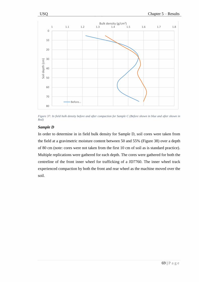
USQ Chapter 5 – Results
69 | P a g e
Figure 37: In field bulk density before and after compaction for Sample C (Before shown in blue and after shown in
Red)
Sample D
In order to determine in in field bulk density for Sample D, soil cores were taken from
the field at a gravimetric moisture content between 50 and 55% (Figure 38) over a depth
of 80 cm (note: cores were not taken from the first 10 cm of soil as is standard practice).
Multiple replications were gathered for each depth. The cores were gathered for both the
centreline of the front inner wheel for trafficking of a JD7760. The inner wheel track
experienced compaction by both the front and rear wheel as the machine moved over the
soil.
0
10
20
30
40
50
60
70
80
1 1.1 1.2 1.3 1.4 1.5 1.6 1.7 1.8
Soil
dep
th (
cm)
Bulk density (g/cm3)
Before…
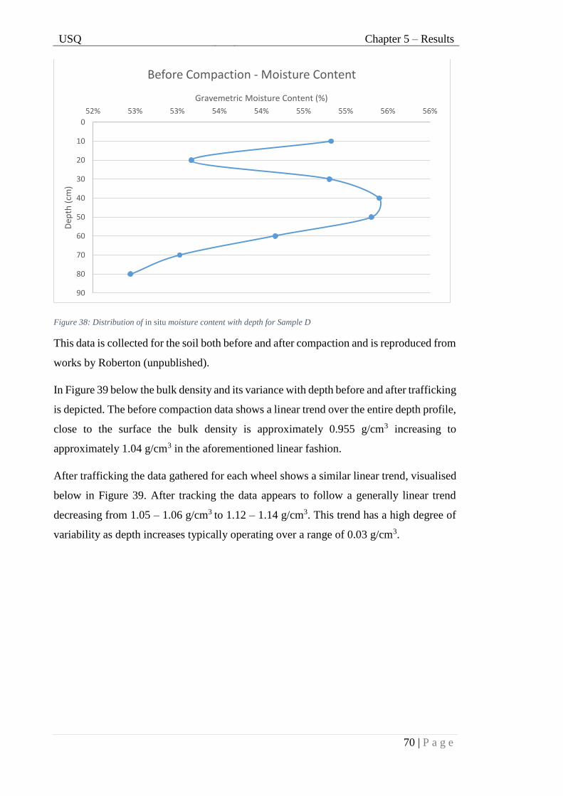
USQ Chapter 5 – Results
70 | P a g e
Figure 38: Distribution of in situ moisture content with depth for Sample D
This data is collected for the soil both before and after compaction and is reproduced from
works by Roberton (unpublished).
In Figure 39 below the bulk density and its variance with depth before and after trafficking
is depicted. The before compaction data shows a linear trend over the entire depth profile,
close to the surface the bulk density is approximately 0.955 g/cm3 increasing to
approximately 1.04 g/cm3 in the aforementioned linear fashion.
After trafficking the data gathered for each wheel shows a similar linear trend, visualised
below in Figure 39. After tracking the data appears to follow a generally linear trend
decreasing from 1.05 – 1.06 g/cm3 to 1.12 – 1.14 g/cm3. This trend has a high degree of
variability as depth increases typically operating over a range of 0.03 g/cm3.
0
10
20
30
40
50
60
70
80
90
52% 53% 53% 54% 54% 55% 55% 56% 56%
Dep
th (
cm)
Gravemetric Moisture Content (%)
Before Compaction - Moisture Content

USQ Chapter 5 – Results
71 | P a g e
Figure 39: In situ distribution of bulk density with depth for Sample D. Before compaction is shown in blue and after
compaction is shown in red
Sample E
The infield bulk density data gathered from this site has received compaction by a JD7760
picking six one meter rows. The tires were inflated at 100% of the recommended pressure
and the machine was set up in a dual wheel configuration. The cores were taken from
both before and after trafficking. The data captured and represented as un-trafficked or
control data has been free from traffic for 15 years and thus represents a true control.
These samples have been taken over a depth of 80 cm (again, excluding the top 10 cm)
with 3 replicates taken for each depth.
As seen below in Figure 40 the bulk density before trafficking typically started at quite a
low bulk density, 0.95 g/cm3, from this point there is a steep linear increase to
approximately 1.15 g/cm3 over approximately 7.5-10cm depth. Following this the
average trend increases linearly from 1.15 g/cm3 to 1.225 g/cm3 over the remaining 70 -
72.5 cm.
Figure 40 below also shows the dry bulk density values after compaction by the JD7760.
The compaction generated at in the inner wheel shows a parabolic relationship between
depth and compaction. The compaction starts at a peak of approximately 1.24 g/cm3 the
bulk density then steadily decreases with depth to a minimal value of 1.18 cm/g3 at 45
cm. From here the bulk density is shown to increase back to the 1.24 g/cm3 which is
similar to the control value of 1.23 g/cm3.
0
10
20
30
40
50
60
70
80
90
0.94 0.96 0.98 1 1.02 1.04 1.06 1.08 1.1 1.12 1.14
Dep
th (
cm)
Bulk Density (g/cm3)
After Before

USQ Chapter 5 – Results
72 | P a g e
Figure 40: In situ distribution of bulk density with depth for Sample E. Before compaction is shown in light blue and
after compaction is shown in dark blue
Summary
As seen across the majority of the soil samples the bulk density is typically at a maximum
at the maximum depth, this maximum varies according to the sample. The moisture
contents were shown to vary greatly and will need to be accounted for in the coming
chapters.
0
10
20
30
40
50
60
70
80
0.95 1.05 1.15 1.25 1.35
Dep
th (
cm)
Bulk Density (g/cm3)
S100-WI Control

USQ Chapter 6 – Evaluation of Modified Methods
73 | P a g e
Chapter 6 – Evaluation of Modified Methods
6.1 Introduction
With the results presented in Chapter 5 it becomes possible to undertake a discussion
examining the highlighted trends and providing reasoning and support for these
occurrences. Once this has occurred a number of comparisons must be made in order to
facilitate the selection of an applicable load and test. This will directly satisfy the aim
stated as: experimental validation and evaluation of modified methods.
In order to achieve this the discussion has been split into five sections discussing: the
results from the Proctor test, the results from the uniaxial test, general comparisons
between the two tests, a brief comparison between the in-situ data and the SoilFlex output,
comparisons between the testing methods and the in-field data, and, finally, selection of
an applicable loading and test.
6.2 Procter Test
6.2.1 Standard Compactive Effort
Most samples tested produced the results that would be expected from the proctor test,
this has allowed the selection of optimum moisture contents and maximum bulk density,
determined by the parabolic trend present. Such a result is demonstrated numerous times
within the literature (Hamza & Anderson 2005, Rollins, Jorgensen & Ross 1998, DAS
2010) as well as with in the relevant Australian Standards (AS1289.5.1.1).
As seen in Table 7 Samples A and F did not produce conclusive results. As earlier
suggested the soil was surpassing its plastic limit and was approaching the liquid limit,
meaning that the apparatus no longer functioned as intended and with each strike
significant volume of sample was remove with the hammer. This prevented the un-
obstructed fall of the hammer, reducing the energy input into the soil. Whilst temporal
constraints limited further investigation of these effects, it is suggested that a lower range
of moisture content would result in a successful outcome. However, such a range would
not be considered typical of Vertosols soil, which the tests were carried out for (Kirby
1991).
As has been discussed within the literature review (University of Southern Queensland
2013) the liquid limit is defined as the moisture content where soil cohesive forces are
completely overcome and the material behaves as a fluid, usually associated with the
pores being completely saturated–super-saturated; this decreases compaction generated

USQ Chapter 6 – Evaluation of Modified Methods
74 | P a g e
by a given force, as well as this the load bearing capacity is severely reduced. When
proctor testing was carried out on Samples A and F the hammer was seen to cause
significant depressions in the soil surface whereby soil was vertically displaced around
the hammer, suggesting that the soil was not capable of supporting the applied load due
to the liquid limit being overcome or proximal. This occurred on close to every blow and
resulted in the clay displaced by the hammer raising up around the edges, coming into
contact with the sides of the proctor testing rig. Hence, this further worsened the
variability of the compactive effort.
Because Samples A and F were excluded from testing it is necessary to investigate the
effects that this may have on the conclusions that are drawn as a result of further testing.
Since whole samples have been excluded as opposed to replacing the test with a different
method of determining the optimum moisture content the only significant impact on the
testing on a whole will be a reduced confidence in any conclusions drawn (as opposed to
inconsistencies in testing methods causing incomparable results). This will only be a
minor loss of confidence as the remaining four samples exhibit strong results over many
replicates allowing substantial weight to be given to any conclusions drawn.
This prompts important questions as to the effect of changing the moisture content over
a larger range of moisture contents. The parabolic function suggests that as the moisture
content increases or decreases outside of the tested range the bulk density reduces to zero
(which would suggest a void) and this is obviously not the case. When utilising the data
extending over a larger set of moisture contents the results indicate a plateau either side
of the maximum dry bulk density, which is commensurate with boundary conditions
occurring. These conditions represent the lowest density achievable which is defined by
void space and gravity, and the specific gravity of the soil constituents (sand, silt and
clay) which is the theoretical density occurring where no void space exists and the total
volume is solid.
6.2.2 Modified Compactive Effort
Testing Samples B through E using the proposed modification of the proctor test for
estimated compactive effort (static load equivalent) provided results with good
confidence and a general logarithmic trend approaching an asymptote well before specific
gravity. However, trend lines reach asymptotic behaviour well beyond the specific gravity
(constant values for all soil constituents), which is impossible. Further testing would be
required to define the bulk density upper limit, but the observed trend is applicable for

USQ Chapter 6 – Evaluation of Modified Methods
75 | P a g e
the observed data representing equivalent static loads well beyond that expected to ever
occur in agricultural fields.
It was noted that at 33 and 69 blows (800 and 1600 kPa estimated equivalent; Raghavan
& Ohu 1985) the sample began to deform and surround the hammer i.e. hammer strikes
one side of the sample caused localised deformation resulting in the other side of the
sample to rise, however this was only by a few millimetres. This was only experienced at
higher loadings and did not present during lower compactive efforts. Such behaviour
should be expected as soils approach the maximum compactive density. However, also
affecting this phenomena is the relationship between OMC and load. soils exhibiting this
have been shown by Rollins et al. (1998), using silty (70%) soil samples, showed that
such behaviour can occur because as the compressive load increases (using the proctor
test) the optimum moisture content becomes slightly smaller, with each increase in load,
and the peak bulk density rises for each small reduction in OMC (Hillel 2004). This
suggests that the optimum moisture content selected from a lower compactive effort
would be greater than the actual optimum moisture content. From the literature review it
is known that moisture contents above the optimum moisture content are not as suited to
bearing loads, especially as the liquid limit becomes proximal (Hillel 2004). When this is
considered it is suggested that this lack of bearing capacity causes also contribute to the
small deformation of the sample.
When examining the results it can be seen that the bulk densities predicted by the model
for higher compactive efforts are generally greater than those experienced in the testing.
Examining the results presented by Rollins et al. (1998) (page 702, Figure 3) it can be
seen that an increase in compactive effort can result in an equal bulk density to that of a
lower compactive effort, suggesting that a more applicable trend would be one where the
bulk density approaches an asymptote. This is not totally provided by the logarithmic
trend but its use over the range tested is applicable in this situation. The use of the
logarithmic trend is supported by Blotz et al (1998) stating similar rationale with clayey
soils.
Another reason the increase in bulk density becomes limited at higher blow counts is due
to the nature of the testing method. The use of impact loads and the differences between
this and static loading have been discussed in the literature review, however the repetitive
application of a small load must be considered. Using the standard proctor test it is known
that each blow has an impact loading of 22.37 kPa (equivalent to an 88.8 kPa static load).

USQ Chapter 6 – Evaluation of Modified Methods
76 | P a g e
Once the soil has reached a certain level of compaction it is plausible that a single impact
of the hammer may not be capable of inducing compaction, thus increasing the number
of blows would not necessarily result in an increase in bulk density past a certain bulk
density. This is seen to add weight to the use of a logarithmic trend that is fitted to the
data; showing the change in bulk density decreasing as the load increases.
The expected discrepancy described above between applied force and the compactive
effort has fuelled the decision to relate the compaction in the proctor tests to the number
of blows as it is more correct than relating it to a net compactive effort, although the two
are linearly related at lower efforts.
6.3 Uniaxial Compression Test
The uniaxial compression test was carried out as per the procedure set out in Chapter 4
(Experimental Procedure) and generally the results showed a logarithmic trend with some
degree of variability between replications.
The reasoning behind the logarithmic trend is mostly the same as for the Proctor Testing
in regards to moisture content although the uniaxial test is not limited by the stepped
loadings provided by the proctor hammer.
As discussed earlier the optimum moisture content decreases as the load on the soil
increases. In the testing that this procedure is based on, Häkansson (1990) uses a drained
cylinder loaded for 2–4 days. After this time period it was found that the optimum
moisture content was reached as a by-product of the draining caused by compaction.
Within this project a drained mould covered with filter paper was used for a loading
period of 5 minutes. Whilst some drainage was experienced during the loading the loading
time was not sufficient to induce enough drainage to reach an optimum moisture content,
this suggests that the same logarithmic style trend is applicable in this case as discussed
when considering the proctor test. However, it is also noted that Suzuki et al (2013)
demonstrated that static loading for short periods (i.e. 5 min) produced densities
comparable to those produced over the 2–4 days. Hence, it may be that whilst the true
OMC for the compactive effort applied is unknown, the trend in density should not be
expected to change significantly, even if load was supplied to its corresponding true bulk
density. On the other hand, a conceptual diagram of a family of proctor curves for
increasing load (Hillel 2004, p251) shows that OMC can have a drastic effect on the
maximum dry density depending on the load. Whilst this appears in direct contradiction
to Suzuki et al. (2013), and the results presented here, the shift of OMC and subsequent

USQ Chapter 6 – Evaluation of Modified Methods
77 | P a g e
magnitude of change in the maximum dry density is a function of the applied load. Thus,
in order to satisfy both observed conditions of Hillel (2004) and Suzuki et al. (2013) it is
suggested the sensitivity to increasing load is not great within the tested range of the
current project.
In testing it was found that the test featured a relatively high degree of variability between
replications. This was found to be due to the design of the testing apparatus: Because a
shop press was used to apply the load, the pressure within the press had to be constantly
altered to match the required loading. This was due to the deformation of the soil: i.e. the
as the soil was compacted the load had to be increased to make up for the corresponding
decrease in load. Because of this the pressure on the soil tended to fluctuate ± 27 kPa
although in some tests (typically in the 1600 kPa test) the load was seen to vary + 53.3
kPa, -27 kPa. This variation is relatively low when compared to the total loading however
it still had effect on the results.
Variability also entered into the testing procedure for the higher loads where some of the
sample was forced up between the load plate and the edge of the mould. This gap was
very small and the occurrence was minimal, but small changes in volume can effect
density substantially. Further variability might have been incurred by the pre-
compression of the soil by the load plate and cell (approximately 2 kg each) although this
is likely to have had close to nil effect on the end result given the loads applied were
significantly greater than this.
6.4 General Comments on the Tests
General comparisons between the two tests can also be made relating to areas such as
reproducibility, ease of testing, time and labour requirements as well as changes to the
tests that may improve the results or the tests relative usefulness.
As mentioned previously the tests for most soils occurred at a moisture content that was
higher than that provided by the initial uniaxial compression test. As suggested in the
literature review this will have a considerable effect on the bulk densities reached by the
tests; typically resulting in values lower than might be expected.
The results gathered indicate that the reproducibility was typically better in the proctor
test when comparing the variance between the replicates at each applied load (Tables 13
– 26 (Appendix H and I)). However, it should be stated that the reproducibility of the
uniaxial test could be vastly increased with some minor modification of the procedure.

USQ Chapter 6 – Evaluation of Modified Methods
78 | P a g e
This modification would see the loading apparatus become computer operated such that
the compressive load is held at relatively constant loading, in addition to this a rubber mat
should be included between the soil and the load plate as suggested by Häkansson (1990).
This mat should be same diameter as the mould or slightly larger such that the sample is
prevented from passing up the side of the load plate. Obtaining a mat for these data with
the required accuracy was outside the logistical constraints of the project.
The time and labour requirements between each test are largely the same with
approximately 10 min required of one operator to collect one data point (this varies for
the proctor test; obviously performing 69 blows a layer takes far more time than 6 blows
per layer). This excludes the preparatory work that must occur first, which includes drying
and moistening the soil to the required moisture contents, but these should be considered
as approximately equal for both tests. Whilst the proctor test does have the same operating
requirements in terms of labour and time it is a much more “hands on” test. The operator
is required to input the compaction to the soil manually using the hammer. This is not a
large issue when a small number of impacts are used however as the blows increase to 69
the operator is required to perform a very repetitive task. This leaves some scope for
possible repetitive strain injuries as discussed in the safety section. In addition to this the
hands on nature of the work leaves a larger scope for operator error (for example:
miscounting number of blows), assuming the load produced by the uniaxial compression
test can be stabilised.
6.5 Compare In-Situ Data with SoilFlex
Comparisons between the data gathered in-situ and the trends produced by SoilFlex in
Chapter 3 can be used to help validate the SoilFlex output produced.
SoilFlex typically produced a logarithmic distribution of stress with depth generating a
change in bulk density that generated a logarithmic change in bulk density with depth.
Chapter 5 (Results) shows the infield bulk density changing logarithmically with depth.
However this trend is mirrored to that predicted by SoilFlex, with the surface of the
sample typically producing a lower bulk density that increases with depth. Conversely,
the bulk density predicted by SoilFlex shows a peak bulk density at the surface of the soil,
decreasing with depth. This is primarily due to two factors: 1) a shallow soil surface that
is highly friable (loose) due to the self-mulching nature of Vertosols (McGarry 1996) and
2) increased strength of surface aggregates due to being much drier (evaporation even at
low temperatures due to atmospheric boundary) meaning much lower moisture content

USQ Chapter 6 – Evaluation of Modified Methods
79 | P a g e
than the soil bulk. In modelling with SoilFlex there factors must be ignored as the model
can only use one assumed moisture content and initial bulk density throughout the soil
profile (Keller et al. 2007).
When the bulk density is considered with a comparison between before and after
compaction values a logarithmic trend is produced that follows the SoilFlex output
closely. This suggests that the SoilFlex model supports the infield bulk densities,
confirming their relevance.
6.6 Comparisons between Tests and In-Situ Bulk Density
Using the information presented above it becomes possible to compare the tested and
infield bulk densities on a case by case basis with the aim of selecting a reference loading
and test. This will be achieved through the use of tables 9 through 12, where the
compaction experienced in field is compared to the bulk density achieved using each
method in the laboratory. The degree of compaction is then calculated using the ration of
in field bulk density to the reference bulk density as presented in the section 2.7. The
infield data shown are the average bulk densities produced by the maximum load cases
in the sampled depth (20cm).
Sample B
Table 9 below shows that the degree of compactness is most applicable using the proctor
test with a compactive effort of between 800 and 1600 kPa. The moisture content at which
the in-situ data was collected is significantly higher than the calculated optimum, this
suggests that it is likely that higher bulk densities could conceivably be achieved under
the right conditions.

USQ Chapter 6 – Evaluation of Modified Methods
80 | P a g e
Table 9: Comparison of laboratory bulk density with in situ bulk density for Sample B
In Situ Laboratory
Load
in
Test
(kPa)
Test
Method
Depth
(cm)
Bulk
Density
(g/cm3)
Moisture
Content
Optimum
Moisture
Content
Bulk
Density
(g/cm3)
Degree of
Compactness
200 Proctor Ave 5
-15 1.47 31% 17%
1.35 109%
Uniaxial 1.00 147%
400 Proctor Ave 5
-15 1.47 31% 17%
1.47 100%
Uniaxial 1.16 126%
600 Proctor Ave 5
-15 1.47 31% 17%
1.53 96%
Uniaxial 1.25 117%
800 Proctor Ave 5
-15 1.47 31% 17%
1.57 93%
Uniaxial 1.32 111%
1600 Proctor Ave 5
-15 1.47 31% 17%
1.67 88%
Uniaxial 1.48 99%
Sample C
The comparison of data for Sample C is provided below in Table 10 and show both the
infield and laboratory moisture contents to be above the optimum of 16%, suggesting that
there is scope for both to generate higher bulk densities.
Table 10: Comparison of laboratory bulk density with in situ bulk density for Sample C
In Situ Laboratory
Load
in
Test
(kPa)
Test
Method
Depth
(cm)
Bulk
Density
(g/cm3)
Moisture
Content
Tested
Moisture
Content
Bulk
Density
(g/cm3)
Degree of
Compactness
200 Proctor Ave 5
-15 1.40 21% 19%
1.34 104%
Uniaxial 0.93 151%
400 Proctor Ave 5
-15 1.40 21% 19%
1.44 98%
Uniaxial 0.97 145%
600 Proctor Ave 5
-15 1.40 21% 19%
1.49 94%
Uniaxial 0.99 142%
800 Proctor Ave 5
-15 1.40 21% 19%
1.52 92%
Uniaxial 1.00 139%
1600 Proctor Ave 5
-15 1.40 21% 19%
1.59 88%
Uniaxial 1.04 134%

USQ Chapter 6 – Evaluation of Modified Methods
81 | P a g e
Sample D
The values presented for Sample D below in Table 11 show the in situ moisture content
to be significantly higher than the optimum moisture content of 28%, suggesting that a
significant increase in bulk density could be expected at optimum conditions. The effect
of this will be somewhat limited by the tested moisture content being 3% higher than the
optimum.
Table 11: Comparison of laboratory bulk density with in situ bulk density for Sample D
In Situ Laboratory
Load
in
Test
(kPa)
Test
Method
Depth
(cm)
Bulk
Density
(g/cm3)
Moisture
Content
Tested
Moisture
Content
Bulk
Density
(g/cm3)
Degree of
Compactness
200 Proctor Ave
10 -20 1.07 53% 31%
1.05 101%
Uniaxial 0.74 144%
400 Proctor Ave
10 -20 1.07 53% 31%
1.09 98%
Uniaxial 0.77 138%
600 Proctor Ave
10 -20 1.07 53% 31%
1.11 96%
Uniaxial 0.79 135%
800 Proctor Ave
10 -20 1.07 53% 31%
1.12 95%
Uniaxial 0.80 132%
1600 Proctor Ave
10 -20 1.07 53% 31%
1.14 93%
Uniaxial 0.84 127%

USQ Chapter 6 – Evaluation of Modified Methods
82 | P a g e
Sample E
The data presented in Table 12 below shows both the tested and in field moisture contents
being equal at 28%, again above the peak of 22%, suggesting the bulk densities listed
could become higher in more optimum conditions.
Table 12: Comparison of laboratory bulk density with in situ bulk density for Sample E
In Situ Laboratory
Load
in
Test
(kPa)
Test
Method
Depth
(cm)
Bulk
Density
(g/cm3)
Moisture
Content
Tested
Moisture
Content
Bulk
Density
(g/cm3)
Degree of
Compactness
200 Proctor Ave 5
-15 1.28 28% 28%
1.06 121%
Uniaxial 0.79 162%
400 Proctor Ave 5
-15 1.28 28% 28%
1.12 114%
Uniaxial 0.81 157%
600 Proctor Ave 5
-15 1.28 28% 28%
1.16 110%
Uniaxial 0.83 155%
800 Proctor Ave 5
-15 1.28 28% 28%
1.18 108%
Uniaxial 0.84 153%
1600 Proctor Ave 5
-15 1.28 28% 28%
1.23 104%
Uniaxial 0.86 149%
6.7 Selection of Applicable Loading/Test
The Tables presented in Tables 9 to 12 above show that the most applicable reference
loading occurs at the 800 or 1600 kPa values through the use of the proctor test. As noted
from the graphs presented in Chapter 5 above the logarithmic trend suggests that causing
a meaningful increase in bulk density from 800 to 1600 kPa and beyond would require
the input of a significantly greater load. As such the selection of 1600 kPa using the
proctor test is logical as it presents the degree of compactness in the most consistently
usable fashion (>90%). The use of 800 kPa is possible and has a lessor labour requirement
however produces a higher degree of compaction (between 2 and 5%). This is a small
change in percentage, however given that higher bulk densities are feasible (as suggested
by the moisture content) it is suggested that the 1600 kPa proctor test will be more
applicable.

USQ Chapter 7 – Conclusions and Future Work
83 | P a g e
Chapter 7 – Conclusions and Future Work
The aim of this project was to investigate the applicability of the standard load used in
the Uniaxial Compression Test to describe the impact of large harvesting machines, such
as the John Deere 7760 cotton picker (JD7760), on the soil. In doing so a number of aims
were identified: review of best practice for measurement of agricultural compaction,
analysis of selected methods and modification of these to suit and assess increased weight
of agricultural machinery and experimental validation and evaluation of modified
methods which have been achieved.
The literature review has identified that the Uniaxial Compression Test with a load of 200
kPa has been used in the pass to generate a reference maximum bulk density. This test
has been used as the Proctor Test was seen to generate a load greater than that typically
experienced under farm machinery.
However, due to a vast increase in the size and weight of farming machinery it is not
uncommon to find soils that have experienced a loading of as much as 600 kPa (JD7760).
This has been confirmed through the use of the SoilFlex model. In doing so; outputs have
been generated to describe the idealised distribution of both the bulk density and stress
with depth as a result of the JD7760 contact pressure. This has shown a stress distribution
of 200 – 600 kPa over a depth of 1m.
This has confirmed the need to either redefine the load used in the Uniaxial Compression
Test or revert to the Proctor Test such that the reference compaction generated is
representative of that experienced in the field. To achieve this, these testes have been
conducted on four Australian Vertosol soils utilising loads of 200, 400, 600, 800 and 1600
kPa. Initial testing was conducted on six soils with inconclusive results produced for the
first and last. These two soils should be re-tested to further validate the results.
Testing found that across all samples and testing the bulk density was related to the
increasing load with a logarithmic trend, this, coupled with the concept of a theoretical
no air voids maximum bulk density suggests that the logarithmic trend would continue
to increase until reaching an asymptote.
These values were then compared to the in-situ bulk densities with consideration made to
the moisture content of the soils at the time of testing. This comparison led to the selection
of 1600 kPa as the most applicable, shown in Tables 9 - 12.

USQ Chapter 7 – Conclusions and Future Work
84 | P a g e
The percentages shown in these tables are higher than would be expected due to a
calculative error inherent in testing causing the moisture content in testing to be higher
than the optimum for most samples, reducing the achievable bulk density for a given load.
As such further testing is required to confirm the data.
Despite this the recommendation of the 1600 kPa proctor test can occur as it produces
data showing the bulk densities that would be most usable in reality. In its selection the
proctor test was compared to the uniaxial test in terms of time, labour requirements and
repeatability. Typically, the proctor test was found to be more reproducible than the
uniaxial test. The repeatability of the uniaxial test could be increased through the
mechanised stabilisation of the applied load. Whilst both test took a similar time to
complete it was found that the uniaxial test was a less labour intensive and had less scope
for operator error, this is as a result of the repetitive loading technique used in the proctor
test.

USQ References
85 | P a g e
References
Alfredo B.J.C. Nhantumbo, AHC 2006, 'Bulk density by Proctor test as a function of
texture for agricultural soils in Maputo province of Mozambique', Soil and Tillage
Research, vol 87, pp. 231-239.
Arvidsson, J:HI 2014, 'Respnse of Different Crops to Soil Compaction- Short Term
Effects in Swedish Field Experiments', Soil & Tillage Research, vol 138, pp. 56-63.
Australian Standards 2003, 'Methods of Testing Soils for Engineering Purposes'.
Awedat, A, Bennett, J, Raine, S & Misra, R 2012, 'Influence of porosity and permeate
suspended clay concentration on clay entrainment within a Red Ferrosol', Joint Australian
and New Zealand Soil Science Conference 2012, Hobart, Tasmania.
B.J. Radford, DFYDMCP 2001, 'Crop Responses to Applied Soil Compaction and to
Compaction Repair Treatments', Soil and Tilalge Research, pp. 157-166.
Barden, RH 2015, 'Cost Savings at the Expense of Quality, Safety, and'.
Bennett, J, Antille, D & Jensen, T 2015, 'Highlighting the importance of CTF for heavy
cotton harvest machinery', International Controlled Traffic Farming conference, Prague.
Bennett, JM, Antille, DL, Jensen, TA & Bailie, C In Prep, 'Assesing the impacts of new
harvesting technologies on cotton through an imapct assesment framework', NCEA
Publication.
Bennett, JM, Woodhouse, NP, Keller, T, Jensen, TA & Antille, DL 2015, 'Advances in
Cotton Harvestign Technology: a review and implications for the John Deere round baler
cotton picker', Journal of Cotton Science, vol 19, pp. 225 - 249.
Blotz, LR, Benson, CH & Boutwell, GP 1998, 'Estimating Optimum Water COntent and
Maximum Dry Unit Weight for Compacted Clays', Journal of Geotechnical and
Geoenvironmental Engineering, pp. 907 - 912.
Boussinesq, J 1885, 'Application des poteniels á l'étude de l'équilibre et du mouvement
des solides élastiques ', Gautiher-Villars, p. 33.
Braunack, MV & Johnston, DB 2014, 'Changes in Cone Resistance due to Cotton Picker
Traffic Harvest on Australian Cotton Soils', Soil and Tillage Research, vol 140, no. 0, pp.
29 - 39.
Carter, MR 1990, 'Relative Measures of Soil Bulk Density To Charecterize Compaction
in Tillage Studies on Fine Sandy Loams', Canadian Journal of Soil Science, vol 70, pp.
425-433.
Carter, MR 1990, 'Relative Mesures of Soil Bulk Density to CHarecterise Compaction in
TIllage Studies on FIne Sandy Loams', Canadian Journal of Soil Science , vol 70, pp.
425-433.
Cerruti, V 1888, 'Sulla Deformazione di un corpo elastico isotroppo per alcune speciali
condisioni ai limiti', Matthematica Acc. r. de'Lincei.

USQ References
86 | P a g e
Cotton Australia 2012, 'THE ECONOMICS OF COTTON IN AUSTRALIA', viewed 15
February 2015, <http://cottonaustralia.com.au/cotton-library/fact-sheets/cotton-fact-file-
the-economics-of-cotton-in-australia>.
CSIRO 2015, 'The Australian Soil Clasification', The Australian Soil Clasification, pp. 1-
5.
da Silva, AP, Kay, BD & Perfect, E 1997, 'Management Versus Inherent Soil Properties
Effects on Bulk Density and Relative Compaction', Soil & Tillage Research, vol 44, pp.
81-93.
Daniells, I, Larson, DL,MDC & Anthony, DTW 1996, 'SOILpak: a successful dedecision
support system for managing the structure of Vertosols under irrigated cotton', Australian
Journal of Soil Research, vol 34, no. 6, pp. 879 - 889.
DAS, BM 2010, Principles of Geotechnical Engineering, 7th edn, Cengage Learning,
United States of America.
Defossez, P & Richard, G 2002, 'Models of Soil Compaction Due to Traffic and their
Evaluation', Soil and Tillage Research, vol 67, no. 1, pp. 41-64.
Delaney, J & Van Niel, K 1999, Geographical Information Systems: An Introduction,
Oxford University Press, Melbourne.
Etana, A, Håkansson, I, Zagal, E & Bucus, S 1999, 'Effects of Tillage Depth on Organic
Carbon COntent and Physical Properties in Five Swedish Soils', Soil & TIlalge Research,
vol 52, pp. 129-139.
Frölich, OK 1934, 'Druckverteilung im Baugrunde', Spriner Verlag, p. 178.
Gassman, PW, Erbach, SW & Melvin, SW 1989, 'Analysis of Track and Wheel
Comapaction', Transactions of teh American Society of Agricultural Engineers, vol 32(1),
pp. 23-29.
Good Year 2015, 'AG TIRES Volume 17', <http://www.titan-
intl.com/files/Agriculture/WebVolume17AgCatalog.pdf>.
Håkansson, I 1990, 'A Method for Cahrecterizing the State of Compactness of the Plough
Layer', Soil and Tilalge Research, vol 16, pp. 105-120.
Håkansson, I 1990, 'A MEthod For Charecterizing the State of Compactness of the Plough
Layer', Soil & Tillage Research, vol 16, pp. 105-120.
Håkansson, I & Lipiec, J 2000, 'A review of the usefulness of relative bulk density values
in studies of soil structure and compaction', Soil & Tillage Research, vol 53, pp. 71-85.
Hamza, MA & Anderson, WK 2005, 'Soil Compaction in Cropping Systems: A Review
of the Nature, Causes and Possible Solutions', Soil & TIllage Research, vol 82, pp. 121-
145.
Hillel, D 1998, 'Environmental Soil Physics: Fundementals, Applications and
Environmental Considerations', Acedemic Press: San Diego.
Hillel, D 2004, 'Introduction to Environmental Soil Physics'.
Huang, M, Liang, T, Wang, L & Zhou, C 2015, 'Effects of No-Tillage Systems on Soil
Physical Properties and Carbon Sequestration Under LOng Term Wheat-Maize Double
Cropping System', Catena, vol 128, pp. 195-202.

USQ References
87 | P a g e
Inge Håkansson, JL 2000, 'A review of the usefullness of relative bulk density values in
studies of soil struture and compaction', Soil & Tillage Research, vol 53, pp. 71-85.
Isbell, RF 2002, 'The Australian Soil Classification Revised Edition', CSIRO Publishing.
John Deere & Company 2015, '7760 Features and Specs',
<https://www.deere.com/en_ASIA/products/equipment/cotton_harvester/7760_cotton_p
icker/7760_cotton_picker.page>.
Jorajuria, D, Draghi, L & Aragon, A 1997, 'The Effect of Vehicle Weight on teh
Distribution of Compaction With Depth and Yeild of Lolium/Trifolium Grassland', Soil
and Tillage Research , pp. 1-12.
Jose Miguel Reichart, LEASSDJRRHIH 2009, 'Reference bulk density and critical degree
of compactness for no till crop production in subtropical highly weathered soils', Soil and
Tillage Research, vol 102, pp. 242-254.
Kahn, Z 2015, 'Compaction of Soil– Process, Necessity and Theory of Compaction',
<http://www.yourarticlelibrary.com/geography/compaction-of-soil-process-necessity-
and-theory-of-compaction/45567/>.
Keller, T (unpublished), 'Short Discription of Soilflex', (unpublished), pp. 1-2.
Keller, T, Defossez, P, Weisskopf, P & Arvidsson, J:RG 2007, 'SoilFlex: A model for
prediction of soil stresses and soil compaction due to agricultural field traffic including a
synthesis of analytical approaches', Soil and Tillage Research, pp. 391-411.
Kirby, JM 1991, 'Critical State Soil Mechanics Parameters and their Variation for
Vertosols in Eastern Australia', Journal of Soil Science, vol 42, no. 3, pp. 487 - 499.
Koolen, AJ & Kuipers, H 1983, 'Agricultural Soil Mechanics', Advanced Series in
Agricultural Sciences , p. 241.
Kuipers, H & Van Ouwerkerk, C 1963, 'Total Pore SPace Estimations in Freshly
Ploughed Soil', Netherlands Journal of Agricultural Science, vol 11, pp. 45-53.
Kulkarni, SS & Bajwa, SG 2005, 'Spectral Response of Coton Canopy to Soil
Compaction', ASAE Meeting Presentation, ASAE, Tampa, Florida.
Lipiec, J & Hatano, R 2003, 'Quantification of Compaction Effects on Soil Physical
Properties and Crop Growth', Geoderma, vol 116, pp. 107-136.
M.A. Hamza, WKA 2005, 'Soil compaction in cropping systems. A review of the nature,
causes and possible solutions', Soil and Tillage Research, vol 82, pp. 121-145.
Manxiang Huang, TLLWCZ 2015, 'Effects of no-tillage systems on soil physical
properties and carbon sequestration under long-term wheat-maize double cropping
system', Catena, vol 128, pp. 195-202.
McConnell, JS, Frizzell, BS & Wilkerson, MH 1989, 'Effect of Soil Compaction and
Subsoil Tillage of two Alfisols on teh growth and yeild of cotton ', Journal of Production
Agriculture , vol 2, no. 2, pp. 140 - 146.
McGarry, D 1990, 'Soil Compaction and Cotton Growth on a Vertosol', Aystralian
Journal of Soil Research, no. 28, pp. 869-77.
McGarry, D 1996, 'The Structure and Grain Size distribution of Vertosols', Vertosols and
Technologies for their Management (Eds N Ahmad and A Mermut: Elsevier.

USQ References
88 | P a g e
McGarry, D, Garcia-Torres, E, Benites, J, Martinez-Vilela, A & Holgado-Cabrera 2003,
'Tillage and Soil Compaction', Conservation Agriculture, pp. `307 - 316.
McKenzie, DC 2001, 'Cotton Root Growth in a Compacted Vertosol (Grey Vertosol) I.
Prediction using Strength Measurements and "limiting Water Ranges"', Australian
Journal of Soil Research , pp. 1157-1168.
Monsanto 2012, 'Bolgard II Technical Manual', pp. 1-41.
Neale, T 2011, 'The Cost of Grain Harvestor Compaction', Precision Agriculture , vol
Accessed: 25/04/2015, pp. http://precisionagriculture.com.au/news-andarticles.
Nhantumbo, ABJC & Cambule, AH 2006, 'Bulk Density by Proctor Test as a Function of
Texture for Agricultural Soils in Maputo Province of Mozambique', Soil & Tillage
Research, vol 87, pp. 231-239.
NSW Agriculture 1998, 'SOILpak for Cotton Growers', NSW Department of Primary
Industires, Sydney.
O'Sullivan, MF & Robertson, EAG 1996, 'Critical State Parameters from intact sampels
of two agricultural soils', Soil and Tillage Research, vol 49, pp. 325 - 335.
Radford, BJ, Bridge, BJ, Davis, RJ, McGarry, D, Pillai, UP, Rickman, JF, Wlash, PA &
Yule, DF 2000, 'Changes in Properties of a Vertosol and Responses of Wheat after
Compaction with Harvester Traffic', Soil and Tillage Research, pp. 155-170.
Raghavan, GSV & Ohu, JO 1985, 'Prediction of Static Equivalent Pressure of Proctor
Compaction Blows', American Society of Agricultural Engineers, pp. 1398-1400.
Raghavan, GSV & Ohu, JO 1985, 'Prediction of Static Equivalent Pressure of Proctor
Compaction Blows', Transaction fo the American Society of Agricultural Engineers, pp.
1398-1400.
Reichert, JM, Susuki, LEAS & Reinert, DJ 2009, 'Reference Bulk Density and Critical
Degree-of-Compactness for No-Till Crop Production in Subtropical Highly Weathered
Soils', Soil & TIllage Research, vol 102, pp. 242-254.
Rollins, KM, Jorgensen, SJ & Ross, TE 1998, 'Optimum Moisture Content for Dynamic
Compaction of Collapsible Soils', Journal of Geotechnical and Environmental
Engineering, pp. 699 - 708.
Söhne, W 1953, 'Druckverteilung im Boden und Bodenverformung unter
Schlepperreifen', Grundlagen der Landtechnik, vol 5, pp. 49 - 63.
Spoor, G, Tijink, FGJ & Weisskopf, P 2003, 'Subsoil COmpaction: Risk, Avoidance,
Identification and Alleviation', Soil Tillage Research, vol 73, no. 1 - 2, pp. 175 - 182.
Suzuki, LEAS, Reichert, JM & Reinert, DJ 2013, 'Degree of Compactness, Soil Physical
Properties and Yield of Soybean in Six Xoils Under No-Tillage ', CSIRO Soil Research,
vol 51, pp. 311-321.
Twerdoff, DA, Chanasyk, DS, Mapfumo, E, Naeth, MA & Baron, VS 1999, 'Impacts of
Forage Grazing and Cultivation on Near-Surface Relative Compaction', Canadian
Journal of Soil Science, vol 79, pp. 465-471.
University of Minnesota 2001, 'SOIL COMPATION; CAUSES EFFECTS AND
CONTROL', vol http://www.extension.umn.edu/agriculture/tillage/soil-compaction/.

USQ References
89 | P a g e
University of Minnesota 2001, 'SOIL COMPATION; CAUSES EFFECTS AND
CONTROL', viewed 14 February 2015,
<http://www.extension.umn.edu/agriculture/tillage/soil-compaction/>.
University of Southern Queensland 2013, Geology and Geomechanics Study Book,
University of Southern Queensland, Toowoomba.
USQ Safe 2015, 'Work Health and Safety Risk Management Procedure', Usq Polict
Library, vol http://policy.usq.edu.au/documents.php?id=13468PL, no. 31/05/15.
Virmani, SM, Sahrawat, KL & Burford, JR 1982, 'Physical and Chemical Properties of
Vertosols and their Mangement', Transaction 12th International COngress of Soil
Science , Symposia Papers, New Delhi, India.
Walsh, P 2002, 'New method yeilds a worms eye view ', Farmign Ahead, vol 132, pp. 16
- 18.
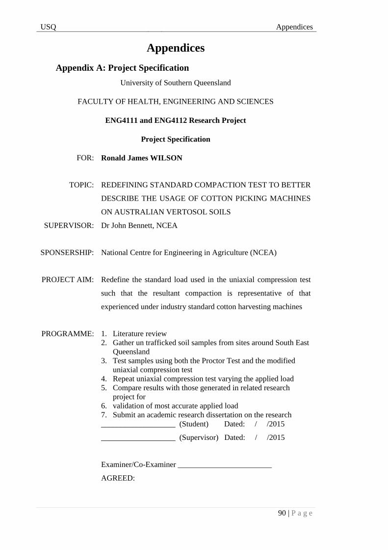
USQ Appendices
90 | P a g e
Appendices
Appendix A: Project Specification
University of Southern Queensland
FACULTY OF HEALTH, ENGINEERING AND SCIENCES
ENG4111 and ENG4112 Research Project
Project Specification
FOR:
TOPIC:
SUPERVISOR:
SPONSERSHIP:
PROJECT AIM:
PROGRAMME:
Ronald James WILSON
REDEFINING STANDARD COMPACTION TEST TO BETTER
DESCRIBE THE USAGE OF COTTON PICKING MACHINES
ON AUSTRALIAN VERTOSOL SOILS
Dr John Bennett, NCEA
National Centre for Engineering in Agriculture (NCEA)
Redefine the standard load used in the uniaxial compression test
such that the resultant compaction is representative of that
experienced under industry standard cotton harvesting machines
1. Literature review
2. Gather un trafficked soil samples from sites around South East
Queensland
3. Test samples using both the Proctor Test and the modified
uniaxial compression test
4. Repeat uniaxial compression test varying the applied load
5. Compare results with those generated in related research
project for
6. validation of most accurate applied load
7. Submit an academic research dissertation on the research
___________________ (Student) Dated: / /2015
___________________ (Supervisor) Dated: / /2015
Examiner/Co-Examiner ________________________
AGREED:

USQ Appendices
91 | P a g e
Appendix B: SoilFlex Flow Chart
Reproduced from Keller et. al. (2007) pp. 395

USQ Appendices
92 | P a g e
Appendix C: SoilFlex Contact Stress Distribution Options
Reproduced from Keller et. al. (2007) pp. 396

USQ Appendices
93 | P a g e
Appendix D: SoilFlex Output
Rear Wheel: Contact Stress
Y
-13
-12 -11 -10 -9 -8 -7 -6 -5 -4 -3 -2 -1 0 1 2 3 4 5 6 7 8 9 10 11 12 13 X
13 22 42 54 42 22
12 41 98 140 169 186 196 186 169 140 98 41
11 28 110 174 223 259 284 298 307 298 284 259 223 174 110 28
10 61 152 224 279 321 351 372 383 391 383 372 351 321 279 224 152 61
9 69 170 251 313 360 396 421 437 447 453 447 437 421 396 360 313 251 170 69
8 51 166 257 327 381 422 451 472 485 493 497 493 485 472 451 422 381 327 257 166 51
7 7 139 244 325 387 433 467 491 508 518 524 528 524 518 508 491 467 433 387 325 244 139 7
6 88 209 304 377 431 471 499 519 532 540 545 548 545 540 532 519 499 471 431 377 304 209 88
5 7 151 264 350 416 464 498 522 538 548 554 558 559 558 554 548 538 522 498 464 416 350 264 151 7
4 63 199 305 385 444 487 517 538 550 558 563 565 566 565 563 558 550 538 517 487 444 385 305 199 63
3 105 235 335 410 465 504 530 547 558 564 567 568 569 568 567 564 558 547 530 504 465 410 335 235 105
2 134 259 355 426 478 514 538 553 562 567 569 570 570 570 569 567 562 553 538 514 478 426 355 259 134
1 151 273 367 436 486 520 543 557 564 568 570 570 570 570 570 568 564 557 543 520 486 436 367 273 151
0 0 156 278 371 439 488 522 544 558 565 568 570 570 570 570 570 568 565 558 544 522 488 439 371 278 156 0
-1 151 273 367 436 486 520 543 557 564 568 570 570 570 570 570 568 564 557 543 520 486 436 367 273 151
-2 134 259 355 426 478 514 538 553 562 567 569 570 570 570 569 567 562 553 538 514 478 426 355 259 134
-3 105 235 335 410 465 504 530 547 558 564 567 568 569 568 567 564 558 547 530 504 465 410 335 235 105
-4 63 199 305 385 444 487 517 538 550 558 563 565 566 565 563 558 550 538 517 487 444 385 305 199 63
-5 7 151 264 350 416 464 498 522 538 548 554 558 559 558 554 548 538 522 498 464 416 350 264 151 7
-6 88 209 304 377 431 471 499 519 532 540 545 548 545 540 532 519 499 471 431 377 304 209 88
-7 7 139 244 325 387 433 467 491 508 518 524 528 524 518 508 491 467 433 387 325 244 139 7
-8 51 166 257 327 381 422 451 472 485 493 497 493 485 472 451 422 381 327 257 166 51
-9 69 170 251 313 360 396 421 437 447 453 447 437 421 396 360 313 251 170 69
-10 61 152 224 279 321 351 372 383 391 383 372 351 321 279 224 152 61
-11 28 110 174 223 259 284 298 307 298 284 259 223 174 110 28
-12 41 98 140 169 186 196 186 169 140 98 41
-13 22 42 54 42 22

USQ Appendices
94 | P a g e
Rear Wheel: Distribution of Stress with Depth

USQ Appendices
95 | P a g e
Rear Wheel: Distribution of Bulk Density with Depth

USQ Appendices
96 | P a g e
Front Wheel: Contact Stress

USQ Appendices
97 | P a g e
Front Wheel: Distribution of Stress with Depth

USQ Appendices
98 | P a g e
Front Wheel: Distribution of Bulk Density with Depth

USQ Appendices
99 | P a g e
Appendix E: Proctor Static Equivalence Table
Number of Blows
(Standard)
Equivalent Static
Load (kPa)
Number of Blows
(Standard)
Equivalent Static
Load (kPa)
1 88.8 31 751.8
2 110.9 32 773.9
3 133 33 796
4 155.1 34 818.1
5 177.2 35 840.2
6 199.3 36 862.3
7 221.4 37 884.4
8 243.5 38 906.5
9 265.6 39 928.6
10 287.7 40 950.7
11 309.8 41 972.8
12 331.9 42 994.9
13 354 43 1017
14 376.1 44 1039.1
15 398.2 45 1061.2
16 420.3 46 1083.3
17 442.4 47 1105.4
18 464.5 48 1127.5
19 486.6 49 1149.6
20 508.7 50 1171.7
21 530.8 51 1193.8
22 552.9 52 1215.9
23 575 53 1238
24 597.1 54 1260.1
25 619.2 55 1282.2
26 641.3 56 1304.3
27 663.4 57 1326.4
28 685.5 58 1348.5
29 707.6 59 1370.6
30 729.7 60 1392.7

USQ Appendices
100 | P a g e
Appendix F: Photos of Testing
Proctor Tests
Figure 41: Image showing the proctor mould filled with uncompacted soil
Figure 42: Image showing the application of the proctor hammer to the soil (before first blow)

USQ Appendices
101 | P a g e
Figure 43: Surface of the soil after proctor compaction has occurred and the sample has been cut at the level of the
mould
Figure 44: Photo from testing showing the clay sticking to the proctor hammer; reducing the compactive effort per
blow

USQ Appendices
102 | P a g e
Uniaxial Test
Figure 45: Picture showing the uniaxial compression test

USQ Appendices
103 | P a g e
Appendix G: USQ Safety Form
Step 1 - Identify the hazards (use this table to help identify hazards then list all hazards in the risk table)
General Work Environment
Sun exposure Water (creek, river, beach, dam) Sound / Noise
Animals / Insects Storms / Weather/Wind/Lightning Temperature (heat, cold)
Air Quality Lighting Uneven Walking Surface
Trip Hazards Confined Spaces Restricted access/egress
Pressure (Diving/Altitude) Smoke
Other/Details:
Machinery, Plant and Equipment
Machinery (fixed plant) Machinery (portable) Hand tools
Laser (Class 2 or above) Elevated work platforms Traffic Control
Non-powered equipment Pressure Vessel Electrical
Vibration Moving Parts Acoustic/Noise
Vehicles Trailers Hand tools
Other/Details:
Manual Tasks / Ergonomics
Manual tasks (repetitive, heavy) Working at heights Restricted space
Vibration Lifting Carrying Pushing/pulling
Reaching/Overstretching Repetitive Movement Bending
Eye strain Machinery (portable) Hand tools
Other/Details:
Biological (e.g. hygiene, disease, infection)
Human tissue/fluids Virus / Disease Food handling
Microbiological Animal tissue/fluids Allergenic
Other/Details:
Chemicals Note: Refer to the label and Safety Data Sheet (SDS) for the classification and management of all chemicals.

USQ Appendices
104 | P a g e
Non-hazardous chemical(s) ‘Hazardous’ chemical (Refer to a completed hazardous chemical risk assessment)
Engineered nanoparticles Explosives Gas Cylinders
Name of chemical(s) / Details:
Critical Incident – resulting in:
Lockdown Evacuation Disruption
Public Image/Adverse Media Issue Violence Environmental Issue
Other/Details:
Radiation
Ionising radiation Ultraviolet (UV) radiation Radio frequency/microwave
infrared (IR) radiation Laser (class 2 or above)
Other/Details:
Energy Systems – incident / issues involving:
Electricity (incl. Mains and Solar) LPG Gas Gas / Pressurised containers
Other/Details:
Facilities / Built Environment
Buildings and fixtures Driveway / Paths Workshops / Work rooms
Playground equipment Furniture Swimming pool
Other/Details:
People issues
Students Staff Visitors / Others
Physical Psychological / Stress Contractors
Fatigue Workload Organisational Change
Workplace Violence/Bullying Inexperienced/new personnel

USQ Appendices
105 | P a g e
Risk register and Analysis
Step 1
(cont)
Step 2 Step 2a Step 3 Step 4
Hazards:
From step 1 or
more if identified
The Risk:
What can happen if exposed to the
hazard with existing controls in place?
Existing Controls:
What are the existing controls that are already in
place?
Risk Assessment:
(use the Risk Matrix on p3)
Consequence x Probability = Risk
Level
Additional controls:
Enter additional controls if required to reduce the
risk level
Risk assessment with
additional controls:
(use the Risk Matrix on p3 – has the
consequence or probability
changed?)
Controls
Implemented?
Yes/No
Consequence Probability Risk
Level
Consequence Probabilit
y
Risk Level
Example
Working in
temperatures over
350 C
Heat stress/heat stroke/exhaustion leading to
serious personal injury/death
Regular breaks, chilled water available, loose clothing,
fatigue management policy.
catastrophic possible high temporary shade shelters, essential tasks only, close
supervision, buddy system
catastrophic unlikely mod Yes
Select a
consequence
Select a
probability
Select a
Risk
Level
Select a
consequence
Select a
probability
Select a
Risk Level
Yes or No
Movement
of dried dirt
resulting in
airbourne
dust
particals
Inhalation of dust
particles causing
respiritory problems
Workplace set up with open
windows and doors etc. to allow
cross breezes to carry away the
dus particles
Moderate Rare Low Conduct pouring of dirt outdoors if cross breeze is
unavailable or where a respiritory if required
Minor Rare Low No

USQ Appendices
106 | P a g e
Step 1
(cont)
Step 2 Step 2a Step 3 Step 4
Hazards:
From step 1 or
more if identified
The Risk:
What can happen if exposed to the
hazard with existing controls in place?
Existing Controls:
What are the existing controls that are already in
place?
Risk Assessment:
(use the Risk Matrix on p3)
Consequence x Probability = Risk
Level
Additional controls:
Enter additional controls if required to reduce the
risk level
Risk assessment with
additional controls:
(use the Risk Matrix on p3 – has the
consequence or probability
changed?)
Controls
Implemented?
Yes/No
Consequence Probability Risk
Level
Consequence Probabilit
y
Risk Level
Example
Working in
temperatures over
350 C
Heat stress/heat stroke/exhaustion leading to
serious personal injury/death
Regular breaks, chilled water available, loose clothing,
fatigue management policy.
catastrophic possible high temporary shade shelters, essential tasks only, close
supervision, buddy system
catastrophic unlikely mod Yes
Shop Press:
Pressure
vessel
Jack on shop press bursts Construction quaity of jack and
safety glasses (hydraulic fluid)
Major Rare Low None Major Rare Low No
Shop Press:
Moving
Parts
Fingers caught inbetween
shop press and sample
Slow movement of moving parts
and operator discretion
Moderate Rare Low None Moderate Rare Low No
Shop Press:
Sample slip
Sample and mould slip
due to high pressures
Restrained sample and distance
between operator and machine
Major Possible Moderate Physical seperation of operator from the shop press Insignificant Rare Low Yes
Shop Press:
Failure
Frame of shop press fails
in spectacular fasion
See above and operator
discresion
Minor Rare Low See above Insignificant Rare Low Yes

USQ Appendices
107 | P a g e
Step 1
(cont)
Step 2 Step 2a Step 3 Step 4
Hazards:
From step 1 or
more if identified
The Risk:
What can happen if exposed to the
hazard with existing controls in place?
Existing Controls:
What are the existing controls that are already in
place?
Risk Assessment:
(use the Risk Matrix on p3)
Consequence x Probability = Risk
Level
Additional controls:
Enter additional controls if required to reduce the
risk level
Risk assessment with
additional controls:
(use the Risk Matrix on p3 – has the
consequence or probability
changed?)
Controls
Implemented?
Yes/No
Consequence Probability Risk
Level
Consequence Probabilit
y
Risk Level
Example
Working in
temperatures over
350 C
Heat stress/heat stroke/exhaustion leading to
serious personal injury/death
Regular breaks, chilled water available, loose clothing,
fatigue management policy.
catastrophic possible high temporary shade shelters, essential tasks only, close
supervision, buddy system
catastrophic unlikely mod Yes
Proctor
Hammer:
Moving
parts
Catch fingers in falling
hammer
Operator discretion and design of
hammer
Minor Rare Low None Minor Rare Low No
Hand Tools Cutting or stabbing of
operator whilst using
tools
Operator discresion Insignificant Unlikely Low None Insignificant Unlikely Low No
Manual
Tasks
Strain or overstreaching
as a result of incorrect
lifting of movement
techniques
Operator has undergone various
lifting techinique safety
presentations and practical
exercises
Minor Unlikely Low None Minor Unlikely Low No

USQ Appendices
108 | P a g e
Step 1
(cont)
Step 2 Step 2a Step 3 Step 4
Hazards:
From step 1 or
more if identified
The Risk:
What can happen if exposed to the
hazard with existing controls in place?
Existing Controls:
What are the existing controls that are already in
place?
Risk Assessment:
(use the Risk Matrix on p3)
Consequence x Probability = Risk
Level
Additional controls:
Enter additional controls if required to reduce the
risk level
Risk assessment with
additional controls:
(use the Risk Matrix on p3 – has the
consequence or probability
changed?)
Controls
Implemented?
Yes/No
Consequence Probability Risk
Level
Consequence Probabilit
y
Risk Level
Example
Working in
temperatures over
350 C
Heat stress/heat stroke/exhaustion leading to
serious personal injury/death
Regular breaks, chilled water available, loose clothing,
fatigue management policy.
catastrophic possible high temporary shade shelters, essential tasks only, close
supervision, buddy system
catastrophic unlikely mod Yes
Repetative
Movements
Proctor test repetative
movements in lifting the
hammer
See above Insignificant Rare Low None Insignificant Rare Low No

USQ Appendices
109 | P a g e
Appendix H: Proctor Test Result Tables
Standard Proctor Tests
Table 13: Raw data from the standard proctor test for Sample A
Standard Proctor Test - 25 Blows - Altering Moisture Content
Sample A - Toobeah, QLD
Required Moisture Content
Moisture Content
(%)
Density (wet)
(kg/m3)
Density Dry
(kg/m3)
Density Dry
(g/cm3)
8% 8.47% 1600 1464 1.46
12% 12.44% 1660 1454 1.45
15% 15.43% 1730 1463 1.46
20% 20.38% 1900 1513 1.51
23% 23.35% 2060 1579 1.58
24% 24.30% 1800 1363 1.36
Table 14: Raw data from the standard proctor test for Sample B
Standard Proctor Test - 25 Blows - Altering Moisture Content
Sample B - Goondiwindi, QLD
Required Moisture Content
Moisture Content
(%)
Density (wet)
(kg/m3)
Density Dry
(kg/m3)
Density Dry (g/cm3)
12% 12.03% 1600 1408 1.41
15% 15.01% 1864 1584 1.58
20% 20.02% 1850 1480 1.48
25% 25.00% 1610 1207 1.21
Table 15: Raw data from the standard proctor test for Sample C
Standard Proctor Test - 25 Blows - Altering Moisture Content
Sample C - Yelarbon, QLD
Required Moisture Content
Moisture Content
(%)
Density (wet)
(kg/m3)
Density Dry
(kg/m3)
Density Dry (g/cm3)
8% 9.51% 1510 1366 1.37
12% 12.01% 1670 1469 1.47
15% 14.98% 1750 1488 1.49
18% 17.97% 1770 1452 1.45
21% 21.00% 1840 1454 1.45
24% 24.01% 1690 1284 1.28
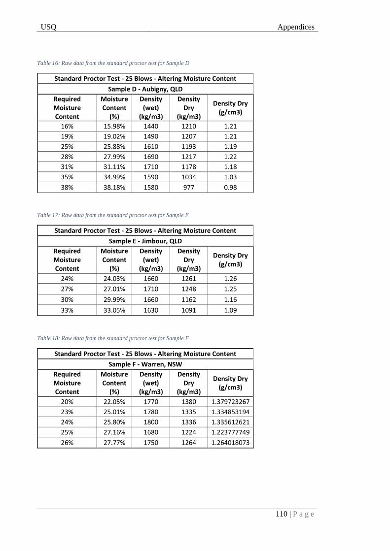
USQ Appendices
110 | P a g e
Table 16: Raw data from the standard proctor test for Sample D
Standard Proctor Test - 25 Blows - Altering Moisture Content
Sample D - Aubigny, QLD
Required Moisture Content
Moisture Content
(%)
Density (wet)
(kg/m3)
Density Dry
(kg/m3)
Density Dry (g/cm3)
16% 15.98% 1440 1210 1.21
19% 19.02% 1490 1207 1.21
25% 25.88% 1610 1193 1.19
28% 27.99% 1690 1217 1.22
31% 31.11% 1710 1178 1.18
35% 34.99% 1590 1034 1.03
38% 38.18% 1580 977 0.98
Table 17: Raw data from the standard proctor test for Sample E
Standard Proctor Test - 25 Blows - Altering Moisture Content
Sample E - Jimbour, QLD
Required Moisture Content
Moisture Content
(%)
Density (wet)
(kg/m3)
Density Dry
(kg/m3)
Density Dry (g/cm3)
24% 24.03% 1660 1261 1.26
27% 27.01% 1710 1248 1.25
30% 29.99% 1660 1162 1.16
33% 33.05% 1630 1091 1.09
Table 18: Raw data from the standard proctor test for Sample F
Standard Proctor Test - 25 Blows - Altering Moisture Content
Sample F - Warren, NSW
Required Moisture Content
Moisture Content
(%)
Density (wet)
(kg/m3)
Density Dry
(kg/m3)
Density Dry (g/cm3)
20% 22.05% 1770 1380 1.379723267
23% 25.01% 1780 1335 1.334853194
24% 25.80% 1800 1336 1.335612621
25% 27.16% 1680 1224 1.223777749
26% 27.77% 1750 1264 1.264018073

USQ Appendices
111 | P a g e
Modified Proctor Tests
Table 19: Raw data from the modified proctor test for Sample B
Proctor Test - Constant Moisture Content - Altering Compactive Effort
Sample B - Goondiwindi, QLD
Number of
Blows
Equivalent Static
Loading (kPa)
Moisture Content (%)
Density (wet)
(kg/m3)
Density Dry (kg/m3)
Density Dry (g/cm3)
6 200 17.02% 1640 1361 1.36
6 200 17.02% 1580 1311 1.31
6 200 17.02% 1540 1278 1.28
15 400 17.02% 1790 1485 1.49
15 400 17.02% 1820 1510 1.51
15 400 17.02% 1800 1494 1.49
25 600 17.02% Calculated 1564 1.56
33 800 17.02% 1890 1568 1.57
33 800 17.02% 1930 1602 1.60
33 800 17.02% 1950 1618 1.62
69 1600 17.02% 1940 1610 1.61
69 1600 17.02% 1970 1635 1.63
69 1600 17.02% 1980 1643 1.64
Table 20: Raw data from the modified proctor test for Sample C
Proctor Test - Constant Moisture Content - Altering Compactive Effort
Sample C - Yelarbon, QLD
Number of
Blows
Equivalent Static
Loading (kPa)
Moisture Content (%)
Density (wet)
(kg/m3)
Density Dry (kg/m3)
Density Dry (g/cm3)
6 200 18.66% 1700 1383 1.38
6 200 18.66% 1530 1244 1.24
15 400 18.66% 1800 1464 1.46
15 400 18.66% 1760 1432 1.43
25 600 18.66% Calculated 1472 1.47
33 800 18.66% 1910 1554 1.55
33 800 18.66% 1950 1586 1.59
33 800 18.66% 1920 1562 1.56
69 1600 18.66% 1970 1602 1.60
69 1600 18.66% 1760 1432 1.43
69 1600 18.66% 2010 1635 1.63

USQ Appendices
112 | P a g e
Table 21: Raw data from the modified proctor test for Sample D
Proctor Test - Constant Moisture Content - Altering Compactive Effort
Sample D - Aubigny, QLD
Number of
Blows
Equivalent Static
Loading (kPa)
Moisture Content (%)
Density (wet)
(kg/m3)
Density Dry (kg/m3)
Density Dry (g/cm3)
6 200 31.17% 1450 1445.49 1.00
6 200 31.17% 1450 1445.49 1.00
15 400 31.17% 1630 1624.93 1.12
15 400 31.17% 1590 1585.06 1.09
15 400 31.17% 1630 1624.93 1.12
25 600 31.17% Calculated 1705.35 1.18
33 800 31.17% 1650 1644.87 1.14
33 800 31.17% 1650 1644.87 1.14
69 1600 31.17% 1620 1614.97 1.11
69 1600 31.17% 1620 1614.97 1.11
69 1600 31.17% 1610 1605.00 1.11
Table 22: Raw data from the modified proctor test for Sample E
Proctor Test - Constant Moisture Content - Altering Compactive Effort
Sample E - Jimbour, QLD
Number of
Blows
Equivalent Static
Loading (kPa)
Moisture Content (%)
Density (wet)
(kg/m3)
Density Dry (kg/m3)
Density Dry (g/cm3)
6 200 28.02% 1450 1445.95 1.04
6 200 28.02% 1450 1445.95 1.04
6 200 28.02% 1430 1426.00 1.03
15 400 28.02% 1590 1585.56 1.14
15 400 28.02% 1590 1585.56 1.14
15 400 28.02% 1560 1555.64 1.12
25 600 28.02% Calculated 1686.62 1.22
33 800 28.02% 1610 1605.50 1.16
33 800 28.02% 1720 1715.19 1.24
33 800 28.02% 1660 1655.36 1.19
69 1600 28.02% 1640 1635.42 1.18
69 1600 28.02% 1670 1665.33 1.20
69 1600 28.02% 1700 1695.25 1.22

USQ Appendices
113 | P a g e
Appendix I: Uniaxial Test Result Tables
Table 23: Raw data from the uniaxial test for Sample B
Uniaxial Compression Test - Constant Moisture Content - Altered Load
Sample B - Goondiwindi, QLD
Load (kPa)
Final Moisture
Content (%)
Density (wet)
(kg/m2)
Density Dry (kg/m2)
Density Dry (g/cm3)
200 16.42% 1354 1351 1.13
200 16.42% 1167 1165 0.98
200 16.31% 1142 1140 0.96
400 16.42% 1461 1458 1.22
400 16.42% 1506 1504 1.26
400 16.31% 1290 1288 1.08
600 16.31% 1348 1345 1.13
600 16.31% 1416 1414 1.19
600 16.31% 1499 1496 1.25
800 16.31% 1440 1438 1.21
800 16.31% 1549 1547 1.30
800 16.31% 1678 1675 1.40
1600 16.31% 1687 1685 1.41
1600 16.31% 1852 1849 1.55
1600 16.31% 1902 1899 1.59 Table 24: Raw data from the uniaxial test for Sample C
Uniaxial Compression Test - Constant Moisture Content - Altered Load
Sample C - Yelarbon, QLD
Load (kPa)
Final Moisture
Content (%)
Density (wet)
(kg/m2)
Density Dry (kg/m2)
Density Dry (g/cm3)
200 18.39% 1101 1099 0.90
200 18.39% 1096 1094 0.89
200 18.39% 1177 1174 0.96
400 18.39% 1111 1108 0.91
400 18.39% 1178 1175 0.96
400 18.39% 1279 1276 1.04
600 18.39% 1217 1214 0.99
600 18.39% 1326 1323 1.08
600 18.39% 1108 1106 0.90
800 18.39% 1242 1239 1.01
800 18.39% 1201 1199 0.98
800 18.39% 1336 1333 1.09
1600 18.39% 1223 1221 1.00
1600 18.39% 1256 1254 1.03
1600 18.39% 1283 1281 1.05

USQ Appendices
114 | P a g e
Table 25: Raw data from the uniaxial test for Sample D
Uniaxial Compression Test - Constant Moisture Content - Altered Load
Sample D - Aubigny, QLD
Load (kPa)
Final Moisture
Content (%)
Density (wet)
(kg/m2)
Density Dry (kg/m2)
Density Dry (g/cm3)
400 30.45% 1095 1092 0.76
400 30.45% 1028 1024 0.71
400 30.45% 1062 1058 0.74
600 30.45% 1202 1198 0.84
600 30.45% 1059 1056 0.74
600 30.45% 1053 1049 0.73
800 30.45% 1064 1061 0.74
800 30.45% 1187 1183 0.83
800 30.45% 1189 1186 0.83
1600 30.45% 1218 1214 0.85
1600 30.45% 1286 1282 0.89
1600 30.45% 1225 1221 0.85
Table 26: Raw data from the uniaxial test for Sample E
Uniaxial Compression Test - Constant Moisture Content - Altered Load
Sample E - Jimbour, QLD
Load (kPa)
Final Moisture
Content (%)
Density (wet)
(kg/m2)
Density Dry (kg/m2)
Density Dry (g/cm3)
200 27.53% 1091 1088 0.79
200 27.53% 1063 1060 0.77
200 27.53% 1062 1059 0.77
400 27.53% 1073 1070 0.78
400 27.53% 1143 1140 0.83
400 27.53% 1164 1161 0.84
600 27.53% 1112 1109 0.81
600 27.53% 1151 1148 0.83
600 27.53% 1203 1200 0.87
800 27.53% 1218 1215 0.88
800 27.53% 1225 1221 0.89
800 27.53% 1109 1106 0.80
1600 27.53% 1089 1086 0.79
1600 27.53% 1209 1206 0.88
1600 27.53% 1186 1183 0.86