Title: Compelling Evidence for a Large ExomoonOrbiting Kepler-1625b

Authors: Alex Teachey,1∗ David M. Kipping1

Affiliations: 1Department of Astronomy, Columbia University in the City of New York

∗E-mail: ateachey@astro.columbia.edu.

One Sentence Summary: HST finds evidence for a large exomoon.

Abstract: Exomoons are the natural satellites of planets orbiting stars outside

our Solar System. We present new observations of a candidate exomoon in the

Kepler-1625b system using the Hubble Space Telescope, carried out on 28-29

October 2017 to validate or refute the moon’s presence. We find compelling

evidence in favor of the moon hypothesis, based on timing deviations and a

reduced flux from the star consistent with a large transiting exomoon. Self-

consistent photodynamical modeling suggests that the planet is likely several

times the mass of Jupiter, while the exomoon has a mass and radius akin to

that of Neptune. If confirmed this represents the first unambiguous detection

of a moon beyond our Solar System.

1

Main Text: The search for exomoons remains in its infancy. To date, there are no confirmed

exomoons in the literature, although an array of techniques have been proposed to detect their

existence, such as microlensing (1–3), direct imaging (4,5), cyclotron radio emission (6), pulsar

timing (7) and transits (8–10). The transit method is particularly attractive however since many

small planets down to lunar radius have already been detected (11), and transits afford repeated

observing opportunities to further study candidate signals.

Previous searches for transiting moons have established that Galilean-sized moons are un-

common at semi-major axes of 0.1 to 1 AU (12). This result is consistent with theoretical work

which has shown that the shrinking Hill sphere (13) and potential capture into evection res-

onances (14) during a planet’s inward migration could efficiently remove primordial moons.

Nevertheless, amongst a sample of 284 transiting planets recently surveyed for moons, one

planet did show some evidence for a large satellite, Kepler-1625b (12). The planet is a Jupiter-

sized validated world (15) orbiting a Solar-mass star (16) close to 1 AU in a likely circular

path (12), making it a prime a priori candidate for moons. Based on this, and the hints seen in

the three transits observed by Kepler, we requested and were awarded time on the Hubble Space

Telescope (HST) to observe a fourth transit expected on 28-29 October 2017. In this work, we

report on these new observations and their impact on the exomoon hypothesis for Kepler-1625b.

Our original analysis was the product of a multi-year survey and thus utilized an earlier

version of the processed photometry released by the Kepler Science Operations Center (SOC).

In that study (12), we used the Simple Aperture Photometry (SAP) from SOC pipeline version

9.0 (17), but the most recent and final data release uses version 9.3. In this work we have

re-analyzed the Kepler data using the revised photometry, which includes updated aperture

contamination factors that also affect our analysis. During this process, we also investigated the

effect of varying the model used to remove long-term trend present in the Kepler data.

We detrended the revised Kepler photometry using five independent methods. The first

2

method is the CoFiAM algorithm (18) which was the approach used in the original study, since

it was specifically designed with exomoon detection in mind. In addition, we considered four

other popular approaches: a polynomial fit, a local line fit, a median filter, and a Gaussian

process (see the Supplementary Materials for a detailed description of each). The detrended

photometry is stable across the different methods (see Figure 1), with a maximum standard

deviation between any two SAP time series of 250 ppm, far below the median formal uncertainty

of ∼ 590 ppm. Although we verified the Presearch Data Conditioning (PDC) version of the

photometry (19, 20) produces similar results (as evident in Figure 1), we ultimately only use

the five SAP reductions in what follows. We produce a “method marginalized” final time series

by taking the median of the ith datum across the five methods and propagating the variance

between them into a revised uncertainty estimate (see the Supplementary Materials for details).

In this way, we produce a robust correction of the Kepler data accounting for differences in

model assumptions.

We fit photodynamical models (21) to the revised Kepler data, using the updated contami-

nation factors from SOC v9.3, prior to introducing the new HST data. Bayesian model selection

reveals only a modest preference for the moon model, with the Bayes factor (K), going from

2 logK = 20.4 in our original study down to just 1.0 now. Detailed investigation reveals that

this is not due to our new detrending approach, as we applied our method marginalized de-

trending to the original v9.0 data and recovered a similar result to our original analysis (see the

Supplementary Materials for details). Instead, it appears that the reduced evidence is largely

caused by the changes in the SAP photometry going from v9.0 to v9.3, and to a lesser degree

by the new contamination factors. This can be seen in Figure 1, where the third transit in par-

ticular experiences a pronounced change between the two versions, and it was this epoch which

displayed the greatest evidence for a moon-like signature in the original analysis.

With a much larger aperture than Kepler, HST is expected to provide several times more pre-

3

cise photometry. Accordingly, the question as to whether Kepler-1625b hosts a large moon or

not should incorporate this new information and in what follows we describe how we processed

the HST data and then combined it with the revised Kepler photometry.

HST monitored the transit of Kepler-1625b occurring on 28-29 October, 2017 with Wide

Field Camera 3 (WFC3). A total of 26 orbits, amounting to some 40 hours, were devoted to

observing the event. The observations consisted of one direct image and 232 exposures using

the G141 grism, a slitless spectroscopy instrument that projects the star’s spectrum across the

CCD. This provides spectral information on the target in the near-infrared from approximately

1.1 to 1.7 microns. Of these 232 exposures, only three were unusable, as they coincided with the

spacecraft’s passage through the South Atlantic Anomaly, at which time HST is forced to use its

less-accurate gyroscopic guidance system. Each exposure lasted roughly 5 minutes, resulting

in about 45 minutes on target per orbit. Images are extracted using standard tools made avail-

able by the Science Telescope Space Institute (STScI) and are described in the Supplementary

Materials.

Native HST time stamps, recorded in the Modified Julian Date (MJDUTC) system, were

converted to Barycentric Julian Date (BJDUTC) for consistency with the Kepler time stamps.

The BJDUTC system accounts for light travel time based on the position of the target and the

observer with respect to the Solar System barycenter at the time of observation. As the position

of HST is constantly changing we set the position of the observer to be the center of the Earth at

the time of observation, for which a small discrepancy of ±23 milliseconds is introduced. This

discrepancy can be safely ignored for our purposes.

While the telescope performed nominally throughout the observation, three well-documented

sources of systematic error are present in our data that require removal. First, thermal fluc-

tuations due to the spacecraft’s orbit lead to clear brightness changes across the entire CCD

(sometimes referred to as “breathing”), which are corrected for by subtracting image-median

4

fluxes (see the Supplementary Materials for details). After computing an optimal aperture for

the target, we observe a strong intra-orbit ramping effect (also known as the “hook”) in the

white light curve (see Figure 2), which has been previously attributed to charge trapping in

the CCD (22, 23). We initially tried a standard parametric approach for correcting these ramps

using an exponential function, but found the result to be sub-optimal. Instead, we devised a

new non-parametric approach described in the Supplementary Materials which substantially

out-performs the previous approach.

We achieve a final mean intra-orbit precision of 375.5 ppm (versus 440.1 ppm using expo-

nential functions), which is approximately 3.8 times more precise than Kepler when correcting

for exposure time. The transit of Kepler-1625b is clearly observed even before the hook cor-

rection. After removal of the hooks, an apparent second decrease in brightness appears towards

the end of the observations, which is evident even in the noisier exponential ramp corrected

data (see Figure 2). Repeating our analysis for the only other bright star fully on the CCD,

KIC4760469, reveals no peculiar behavior at this time indicating that the dip is not due to an

instrumental common mode. Similarly, the centroids of both the target and the comparison star

show no anomalous change around this time (see figure in the Supplementary Materials). (

By correlating the observed centroid variations with flux for both the target and the com-

parison star, we estimate that the small centroid changes in the second visit should induce (via

residual pixel sensitivity variations) a flux change of ∼20 ppm, and certainly < 100 ppm (see

figure in the Supplementary Materials). Since the moon-like dip is∼500 ppm, it appears highly

improbable that this could explain the apparent dip. In conclusion, although we cannot abso-

lutely claim the moon-like dip is not due to an instrumental effect, we have shown that neither an

instrumental common mode nor a residual pixel sensitivity effect can explain the dip and thus

we proceed under the assumption it is astrophysical in what follows (see the Supplementary

Materials for more details on these tests).

5

Upon inspection of the HST images we identified a previously uncatalogued point source

within 2 arcseconds of our target. The star resides at position angle 8.5 degrees East of North,

with a derived Kepler magnitude of 22.65. Its faintness means that it produces negligible con-

tamination to our target spectrum. We attribute its new identification to the fact that it is both

exceptionally faint and so close to the target that it was always lost in the glare in other images.

Utilizing a Gaia-derived distance to the target we find that, were this point source to be at the

same distance, it would be within 4500 AU of Kepler-1625. It is not known if the two sources

are physically associated, however. We estimate that the source contributes less than 1 part in

3000 to our final WFC3 white light curve and thus can be safely ignored.

In addition to the breathing and the hooks, a third well-known source of WFC3 system-

atic error we see is a visit-long trend (apparent in Figure 2). These trends have not yet been

correlated to any physical parameter related to the WFC3 observations (24), and thus the con-

ventional approach is a linear slope (e.g. (25–27)) although a quadratic model has been used

in some instances (e.g. (28, 29)). The timescale of the variations are comparable to the transit

itself and thus cannot be removed in isolation, rather any detrending model is expected to be

covariant with the transit model. For this reason, it was necessary to perform the detrending

regression simultaneous to the actual transits fits. We considered three possible trend models;

linear, quadratic and exponential. All models include an extra parameter describing a flux offset

between the 14th and 15th orbits. This is motivated by the fact that the spacecraft performed a

full guide star acquisition at the beginning of the 15th orbit (a new “visit”), and ends up plac-

ing the spectrum ∼0.1 pixels away from where it appeared during the first 14 orbits. Although

the white light curve shows no obvious flux change at this time, the reddest channels display

substantial shifts motivating this offset term.

Finally, we extract light curves in nine wavelength bins across the spectrum in an attempt to

perform transmission spectroscopy. As a planet transits its host star, the atmosphere may absorb

6

different amounts of light depending on the constituent molecules and their abundances (30).

This makes the planet’s transit depth wavelength-dependent. An accurate measurement of these

transit depths not only provides the potential to characterize the atmosphere’s composition; it

is also potentially useful in providing an independent measurement of the planet’s mass (31).

While a low surface gravity planet will show very pronounced molecular features and a steep

slope at short wavelengths due to Rayleigh scattering, a high surface gravity world will yield a

substantially flatter transmission spectrum.

With the HST WFC3 data prepared, we are ready to combine it with the revised Kepler data

in order to regress candidate models and compare between them. We considered four different

transit models, which when combined with three different visit-long trend models, leads to a

total of 12 models to evaluate. The four transit models here were designated as P, for the planet-

only model; T, for a model that fits the observed transit timing variations (TTVs) in the system

agnostically; Z, for a zero-radius moon model, which may produce all the gravitational effects

of an exomoon without the flux reductions of a moon transit; and M, which is the full planet plus

moon model. Models are generated using the LUNA photodynamical software package (21) and

regression is performed via the multimodal nested sampling algorithm MULTINEST (32, 33).

For each model, we not only derive the joint a posteriori parameter samples, but also a Bayesian

evidence (also known as the marginal likelihood) enabling direct calculation of the Bayes factor

between models.

One clear result from our analysis is that the HST transit of Kepler-1625b occurred '72

minutes earlier than expected, indicating transit timing variations in the system. Bayes factors

between models P and T support this for any choice of detrending model (see Table 1), with the

T fits returning a χ2 decreased by 17 to 19 (for 1048 data points). Further, if we fit the Kepler

data in isolation and make predictions for the HST transit time, the observed time is > 3σ

discrepant (see figure in the Supplementary Materials). Identifying TTVs was among the first

7

methods proposed to discover exomoons (8), but certainly perturbations from an unseen planet

could also be responsible. We find that the '25 minute amplitude TTV can be explained by an

external perturbing planet (see the Supplementary Materials), though with only four transits on

hand it is not possible to constrain the mass or location of such a planet, and no other planet has

been observed so far in the system.

We also found that model Z consistently out-performs model T, though the improvement to

the fits is smaller at ∆χ2 ' 2-5 (see Table 1). This suggests that the evidence for the moon based

on timing effects alone goes beyond the TTVs, providing modest evidence in favor of additional

dynamical effects such as duration changes (9) and/or impact parameter variation (10), both

expected consequences of a moon present in the system. This by itself would not constitute a

strong enough case for a moon detection claim, but we consider it to be an important additional

check that a real exomoon would be expected to pass.

The most compelling piece of evidence for an exomoon would be an exomoon transit, in

addition to the observed TTV. If Kepler-1625b’s early transit were indeed due to an exomoon,

then we should expect the moon to transit late on the opposite side of the barycenter. The

previously mentioned existence of an apparent flux decrease towards the end of our observations

is therefore where we would expect it to be under this hypothesis. Although we have established

that this dip is most likely astrophysical, as yet we have not discussed its significance, nor its

compatibility with a self-consistent moon model.

We find that our self-consistent planet+moon models (M) always out-perform all other tran-

sit models in terms of maximum likelihood and Bayesian evidences (see Table 1). The presence

of a TTV and an apparent decrease in flux at the correct phase position together make for a

compelling case for an exomoon at this point. However, as is apparent from Figure 3, the am-

plitude and shape of the putative exomoon transit varies somewhat between the trend models,

leading to both distinct model evidences and associated system parameters.

8

Although the overall preference of the moon model is arguably best framed by comparison

to model P, the significance of the moon-like transit alone is best framed by comparing M and Z

alone. Such a comparison reveals a strong dependency on the implied significance to the trend

model used. In the worst case, we have the quadratic model with 2 logK ' 4, corresponding to

“positive evidence” (34) - although we note the absolute evidence ZM is the worst amongst the

three. The linear model is far more optimistic yielding 2 logK ' 18, corresponding to “very

strong evidence” (34), whereas the exponential sits between these extremes. The question then

arises, which of our trend models is the correct one?

Because the linear model is a nested version of the quadratic model, and both models are

linear with respect to time, it is more straight-forward to compare these two. The quadratic

model essentially recovers the linear model, apparent from Figure 3, with a curvature within

1.5σ of zero, and yields almost the same best χ2 score to within 1.2. This lack of meaningful

improvement causes the log evidence to drop by 2.8, since evidences penalize wasted prior

volume. The exponential model appears more competitive with a log evidence 1.72 lower, but a

direct comparison of two different classes of models, such as these, is muddied by the fact that

such analyses are sensitive to the choice of priors. The most useful comparison here is simply

to state that the maximum likelihoods are within ∆χ2 = 0.68 of one another and thus are likely

equally justified from data-driven perspective.

Another approach we considered is to weigh the trend models uses the posterior samples.

Given a planet or moon’s mass, there is probabilistic range of expected radii based on empir-

ical mass-radius relations (35). Although we exclude extreme densities in our fits, parameters

from model M can certainly lead to improbable solutions with regards to the photodynamically

inferred (36) masses and radii.

To investigate this, we inferred the planetary mass using two methods for each model and

evaluated their self-consistency. The first method combines the photodynamically-inferred

9

planet-to-star mass ratio (36) with a prediction for the mass based on the well-constrained ra-

dius using forecaster; an empirical probabilistic mass-radius relation (35). The second

method approaches the problem from the other side, taking the moon’s radius and predicting

its mass with forecaster then calculating the planetary mass via the photodynamically-

inferred moon-to-planet mass ratio. Our analysis (discussed in more detail in the Supplemen-

tary Materials) reveals that all three models have physically plausible solutions and generally

converge at ∼103M⊕ for the planetary mass, with the exception of the quadratic model had

broader support extending down to Saturn-mass. We ultimately combined the two mass esti-

mates to provide a final best-estimate for each model in Table 2.

As a consistency check, we used our derived transmission spectrum to constrain the al-

lowed range of planetary masses for a cloudless atmosphere (31). Using an MCMC with

Exo-Transmit (38), we find masses in the range of > 0.4 Jupiter masses (to 95% confi-

dence) are consistent with the nearly flat spectrum observed, assuming a cloudless atmosphere

(see the Supplementary Materials for details).

In conclusion, the linear and exponential models appear to be the most justified by the data

and also lead to slightly improved physical self-consistency, although we certainly cannot ex-

clude the quadratic model at this time. For this reason, we elected to present the associated

system parameters resulting from all three models in Table 2. The maximum a posteriori solu-

tions from each, using model M, are presented in Figure 4 for reference.

We briefly comment on some of the inferred physical parameters for this system. First, we

have assumed a circular moon orbit throughout due to the likely rapid effects of tidal circular-

ization. However, we did allow the moon to explore three-dimensional orbits and find some

evidence for non-coplanarity. Our solution favors a moon orbit tilted by about 45 degrees to

the planet’s orbital plane, with both pro- and retrograde solutions being compatible. The only

comparable known large moon with such an inclined orbit is Triton around Neptune, which is

10

generally thought to be a captured Kuiper Belt object (39). However, we caution that the con-

straints here are weak, reflected by the posterior’s broad shape, and thus it would be unsurprising

if the true answer is in fact coplanar.

One jarring aspect of the system is the sheer scale of it. The exomoon has a radius of

'4R⊕, making it very similar to Neptune or Uranus in size. The measured mass, including

the forecaster constraints, comes in at log(MS/M⊕) = (1.2 ± 0.3)M⊕, which is again

compatible with Neptune or Uranus (although note that this solution is in part informed by

an empirical mass-radius relation). This Neptune-like moon orbits a planet with a size fully

compatible with that of Jupiter at (11.4 ± 1.5)R⊕, but most likely a few times more massive.

Finally, although the moon’s period is highly degenerate and multimodal, we find the semi-

major axis is relatively wide at '40 planetary radii. With a Hill radius of (200± 50) planetary

radii, this is well within the Hill sphere and expected region of stability.

The blackbody equilibrium temperature of the planet and moon, assuming zero albedo, is

∼350 K. Adopting a more realistic albedo can drop this down to∼ 300 K. Of course, as a likely

gaseous pair of objects there is not much prospect of habitability here, although it appears that

the moon can indeed be in the temperature zone for optimistic definitions of the habitable zone.

What is particularly interesting about the star is that it appears to be a Solar mass star evolv-

ing off the main sequence. This inference is supported a recent analysis of the Gaia DR2 par-

allax by (40), as well as our own isochrone fits (see the Supplementary Materials). We find that

the star is certainly older than than Sun, at '10 Gyr in age, and that insolation at the location

of the system was thus lower in the past. The luminosity was likely close to Solar for most of

the star’s life, making the equilibrium temperature drop down to ∼250 K for Jovian albedos for

most of its existence. The old age of the system also implies plenty of time for tidal evolution,

which could explain why we find the moon at a fairly wide orbital separation.

The origins of such a system can only be speculated upon at this time. A mass ratio of 1.5%

11

is certainly not unphysical from in-situ formation using gas-starved disk models, but it does

represent the very upper end of what numerical simulations form (37). In such a scenario, a

separate explanation for the tilt would be required. Impacts between gaseous planets leading

to captured moons is not well-studied but could be worth further investigation. A binary ex-

change mechanism would be challenged by the requirement for a Neptune to be in an initial

binary with comparably mass object, such as a Super-Earth (39). Formation of an initial binary

planet, perhaps through tidal capture, seems improbable due to the tight orbits simulation work

tends to produce from such events (41). If confirmed, Kepler-1625b-i will certainly provide an

interesting puzzle for theorists to solve.

Taken together, a detailed investigation of a suite of models tested in this work suggest that

the exomoon hypothesis is the best explanation to the presently available observations. The

two main pieces of information driving this result are i) a strong case for TTVs, in particular a

72 minute early transit observed during our HST observations and ii) a moon-like transit signa-

ture apparent even in the pre-detrended data. We also note that we find a modestly improved

evidence when including additional dynamical effects induced by moons aside from TTVs.

The exomoon hypothesis is further strengthened by our analysis which demonstrates that a)

the moon-like transit is not due to an instrumental common mode nor residual pixel sensitivity

variations; b) the moon-like transit occurs at the correct phase position to also explain the ob-

served TTV; and c) simultaneous detrending and photodynamical modeling retrieves a solution

which is not only favored by the data, but is also physically self-consistent.

Put together, these points make for a compelling case for an exomoon around Kepler-1625b.

It also represents the simplest hypothesis to explain both the TTV and the post-transit flux

decrease, since other solutions would require two separate and unconnected explanations for

these two observations.

There remains some aspects of our present interpretation of the data that give us pause.

12

First, the moon’s Neptunian size and inclined orbit are peculiar, though it is difficult to assess

how likely this is a priori since no previously known exomoons exist. Second, the moon’s

transit occurs towards the end of the observations and more out-of-transit data could have more

cleanly resolved this signal. Nevertheless, we highlight that no centroid shifts nor flux changes

in our comparison star are found around this time, and thus the dip appears astrophysical in

nature. Third, the moon’s inferred properties are sensitive to the model used for correcting

HST’s visit-long trend and thus some uncertainty remains regarding the true system properties.

However, the solution we deem most likely, a linear visit-long trend, also represents the most

widely agreed upon solution for the visit-long trend in the literature.

Finally, it is somewhat ironic that the case for observing Kepler-1625b with HST was con-

tingent on a previous data release of the Kepler photometry which indicated a moon (12), while

the most recent data release only modestly favors that hypothesis when treated in isolation. De-

spite this, we would argue that planets like Kepler-1625b were always ideal targets for exomoon

follow-up, being a Jupiter-sized planet on a wide, circular orbit around a Solar-mass star. There

are certainly hints of the moon present even in the revised Kepler data, but it is the HST data

- with a precision four times superior to Kepler- which is critical to the driving the moon as

the favored model. These points suggest that it would be worthwhile to pursue similar Kepler

planets for exomoons with HST or other facilities, even if the Kepler data alone do not show

large moon-like signatures. Furthermore, our work demonstrates how impactful the changes to

Kepler photometry were, at least in this case, as it suggests other results over the course of the

Kepler mission may be similarly impacted, particularly for small signals.

All in all, it is difficult to assign a precise probability to the reality of Kepler-1625b-i. For-

mally, the preference for the moon model over the planet-only model is very high, with a Bayes

factor exceeding 400,000. On the other hand, this is a complicated and involved analysis where

a minor effect unaccounted for, or anomalous artefact, could potentially change our interpreta-

13

tion. In short, it is the unknown unknowns that we cannot quantify. These reservations exist

because this would be a first of its kind detection - the first exomoon. Historically, the first exo-

planet claims faced great skepticism because there was simply no precedence for them. If many

more exomoons are detected in the coming years with similar properties to Kepler-1625b-i, it

would hardly be a controversial claim to add one more. Ultimately, Kepler-1625b-i cannot be

considered confirmed until it has survived the long scrutiny of many years, observations and

community skepticism, as well as perhaps the detection of similar such objects. Despite this,

it is an exciting reminder of how little we really know about distant planetary systems and the

great spirit of discovery exoplanetary science embodies.

14

References and Notes

1. Han, C., Han, W. 2002. On the Feasibility of Detecting Satellites of Extrasolar Planets via

Microlensing. The Astrophysical Journal 580, 490.

2. Han, C. 2008. Microlensing Detections of Moons of Exoplanets. The Astrophysical Journal

684, 684.

3. Liebig, C. 2010. Detectability of Extrasolar Moons as Gravitational Microlenses. Astron-

omy & Astrophysics 520, 68.

4. Cabrera, J., Schneider, J. 2007. Detecting companions to extrasolar planets using mutual

events. Astronomy and Astrophysics 464, 1133.

5. Agol, E., Jansen, T., Lacy, B., Robinson, T. D., Meadows, V. 2015. The Center of Light:

Spectroastrometric Detection of Exomoons. The Astrophysical Journal 812, 5.

6. Noyola, J. P., Satyal, S., Musielak, Z. E. 2014. Detection of Exomoons through Observation

of Radio Emissions. The Astrophysical Journal 791, 25.

7. Lewis, K. M., Sackett, P. D., Mardling, R. A. 2008. Possibility of Detecting Moons of

Pulsar Planets through Time-of-Arrival Analysis. The Astrophysical Journal 685, L153.

8. Sartoretti, P., Schneider, J. 1999. On the detection of satellites of extrasolar planets with the

method of transits. Astronomy and Astrophysics Supplement Series 134, 553.

9. Kipping, D. M. 2009. Transit timing effects due to an exomoon. Monthly Notices of the

Royal Astronomical Society 392, 181.

10. Kipping, D. M. 2009. Transit timing effects due to an exomoon - II. Monthly Notices of the

Royal Astronomical Society 396, 1797.

15

11. Barclay, T., and 57 colleagues 2013. A sub-Mercury-sized exoplanet. Nature 494, 452.

12. Teachey, A., Kipping, D. M., Schmitt, A. R. 2018. HEK. VI. On the Dearth of Galilean

Analogs in Kepler, and the Exomoon Candidate Kepler-1625b I. The Astronomical Journal

155, 36.

13. Namouni, F. 2010. The Fate of Moons of Close-in Giant Exoplanets. The Astrophysical

Journal 719, L145.

14. Spalding, C., Batygin, K., Adams, F. C. 2016. Resonant Removal of Exomoons during

Planetary Migration. The Astrophysical Journal 817, 18.

15. Morton, T. D., and 7 colleagues 2016. False Positive Probabilities for all Kepler Objects of

Interest: 1284 Newly Validated Planets and 428 Likely False Positives. The Astrophysical

Journal 822, 86.

16. Mathur, S., and 16 colleagues 2017. Revised Stellar Properties of Kepler Targets for the

Q1-17 (DR25) Transit Detection Run. The Astrophysical Journal Supplement Series 229,

30.

17. Jenkins, J. M., and 29 colleagues 2010. Overview of the Kepler Science Processing

Pipeline. The Astrophysical Journal 713, L87.

18. Kipping, D. M., Hartman, J., Buchhave, L. A., Schmitt, A. R., Bakos, G. A., Nesvorny, D.

2013. The Hunt for Exomoons with Kepler (HEK). II. Analysis of Seven Viable Satellite-

hosting Planet Candidates. The Astrophysical Journal 770, 101.

19. Stumpe, M. C., and 10 colleagues 2012. Kepler Presearch Data Conditioning

I—Architecture and Algorithms for Error Correction in Kepler Light Curves. Publications

of the Astronomical Society of the Pacific 124, 985.

16

20. Smith, J. C., and 10 colleagues 2012. Kepler Presearch Data Conditioning II - A Bayesian

Approach to Systematic Error Correction. Publications of the Astronomical Society of the

Pacific 124, 1000.

21. Kipping, D. M. 2011. LUNA: an algorithm for generating dynamic planet-moon transits.

Monthly Notices of the Royal Astronomical Society 416, 689.

22. Agol, E., and 6 colleagues 2010. The Climate of HD 189733b from Fourteen Transits and

Eclipses Measured by Spitzer. The Astrophysical Journal 721, 1861.

23. Berta, Z. K., and 9 colleagues 2012. The Flat Transmission Spectrum of the Super-Earth

GJ1214b from Wide Field Camera 3 on the Hubble Space Telescope. The Astrophysical

Journal 747, 35.

24. Wakeford, H. R., Sing, D. K., Evans, T., Deming, D., Mandell, A. 2016. Marginalizing

Instrument Systematics in HST WFC3 Transit Light Curves. The Astrophysical Journal

819, 10.

25. Huitson, C. M., and 16 colleagues 2013. An HST optical-to-near-IR transmission spectrum

of the hot Jupiter WASP-19b: detection of atmospheric water and likely absence of TiO.

Monthly Notices of the Royal Astronomical Society 434, 3252.

26. Ranjan, S., and 6 colleagues 2014. Atmospheric Characterization of Five Hot Jupiters with

the Wide Field Camera 3 on the Hubble Space Telescope. The Astrophysical Journal 785,

148.

27. Knutson, H. A., and 9 colleagues 2014. Hubble Space Telescope Near-IR Transmission

Spectroscopy of the Super-Earth HD 97658b. The Astrophysical Journal 794, 155.

17

28. Stevenson, K. B., and 7 colleagues 2014. Transmission Spectroscopy of the Hot Jupiter

WASP-12b from 0.7 to 5 µm. The Astronomical Journal 147, 161.

29. Stevenson, K. B., Bean, J. L., Fabrycky, D., Kreidberg, L. 2014. A Hubble Space Telescope

Search for a Sub-Earth-sized Exoplanet in the GJ 436 System. The Astrophysical Journal

796, 32.

30. Seager, S., Sasselov, D. D. 2000. Theoretical Transmission Spectra during Extrasolar Giant

Planet Transits. The Astrophysical Journal 537, 916.

31. de Wit, J., Seager, S. 2013. Constraining Exoplanet Mass from Transmission Spectroscopy.

Science 342, 1473.

32. Feroz, F., Hobson, M. P. 2008. Multimodal nested sampling: an efficient and robust al-

ternative to Markov Chain Monte Carlo methods for astronomical data analyses. Monthly

Notices of the Royal Astronomical Society 384, 449.

33. Feroz, F., Hobson, M. P., Bridges, M. 2009. MULTINEST: an efficient and robust Bayesian

inference tool for cosmology and particle physics. Monthly Notices of the Royal Astro-

nomical Society 398, 1601.

34. Kass, R. E. & Raftery, A. E. 1995. Bayes Factors. Journal of the American Statistical

Association, 90, 773.

35. Chen, J., Kipping, D. 2017. Probabilistic Forecasting of the Masses and Radii of Other

Worlds. The Astrophysical Journal 834, 17.

36. Kipping, D. M. 2010. How to weigh a star using a moon. Monthly Notices of the Royal

Astronomical Society 409, L119.

18

37. Cilibrasi, M., Szulagyi, J., Mayer, L., Drazkowska, J., Miguel, Y., Inderbitzi, P. 2018.

Satellites Form Fast & Late: a Population Synthesis for the Galilean Moons. ArXiv e-prints

arXiv:1801.06094.

38. Kempton, E. M.-R., Lupu, R., Owusu-Asare, A., Slough, P., Cale, B. 2017. Exo-Transmit:

An Open-Source Code for Calculating Transmission Spectra for Exoplanet Atmospheres of

Varied Composition. Publications of the Astronomical Society of the Pacific 129, 44402.

39. Agnor, C. B., Hamilton, D. P. 2006. Neptune’s capture of its moon Triton in a binary-planet

gravitational encounter. Nature 441, 192.

40. Berger, T. A., Huber, D., Gaidos, E., van Saders, J. L. 2018. Revised Radii of Kepler Stars

and Planets using Gaia Data Release 2. ArXiv e-prints arXiv:1805.00231.

41. Ochiai, H., Nagasawa, M., Ida, S. 2014. Extrasolar Binary Planets. I. Formation by Tidal

Capture during Planet-Planet Scattering. The Astrophysical Journal 790, 92.

42. Dalba, P. A., Muirhead, P. S., Croll, B., Kempton, E. M.-R. 2017. Kepler Transit Depths

Contaminated By a Phantom Star. The Astronomical Journal 153, 59.

43. Bryson, S. T., and 10 colleagues 2010. The Kepler Pixel Response Function. The Astro-

physical Journal 713, L97.

44. Schlafly, E. F., Finkbeiner, D. P. 2011. Measuring Reddening with Sloan Digital Sky Survey

Stellar Spectra and Recalibrating SFD. The Astrophysical Journal 737, 103.

45. Kummel, M., Walsh, J. R., Pirzkal, N., Kuntschner, H., Pasquali, A. 2009. The Slitless

Spectroscopy Data Extraction Software aXe. Publications of the Astronomical Society of

the Pacific 121, 59.

19

46. Bertin, E., Arnouts, S. 2010. SExtractor: Source Extractor. Astrophysics Source Code Li-

brary ascl:1010.064.

47. Kummel, M., Kuntschner, H., Walsh, J. R., Bushouse, H. 2011. Master sky images for the

WFC3 G102 and G141 grisms.Space Telescope WFC Instrument Science Report.

48. Jones, E., Oliphant, T., Peterson, P., et al. 2001, http://www.scipy.org

49. Deming, D., and 20 colleagues 2013. Infrared Transmission Spectroscopy of the Exoplanets

HD 209458b and XO-1b Using the Wide Field Camera-3 on the Hubble Space Telescope.

The Astrophysical Journal 774, 95.

50. Deming, D., Harrington, J., Seager, S., Richardson, L. J. 2006. Strong Infrared Emission

from the Extrasolar Planet HD 189733b. The Astrophysical Journal 644, 560.

51. Knutson, H. A., and 8 colleagues 2007. A map of the day-night contrast of the extrasolar

planet HD 189733b. Nature 447, 183.

52. Charbonneau, D., and 7 colleagues 2008. The Broadband Infrared Emission Spectrum of

the Exoplanet HD 189733b. The Astrophysical Journal 686, 1341.

53. Freedman, R. S., Marley, M. S., Lodders, K. 2008. Line and Mean Opacities for Ultracool

Dwarfs and Extrasolar Planets. The Astrophysical Journal Supplement Series 174, 504.

54. Freedman, R. S., Lustig-Yaeger, J., Fortney, J. J., Lupu, R. E., Marley, M. S., Lodders, K.

2014. Gaseous Mean Opacities for Giant Planet and Ultracool Dwarf Atmospheres over

a Range of Metallicities and Temperatures. The Astrophysical Journal Supplement Series

214, 25.

55. Lupu, R. E., and 8 colleagues 2014. The Atmospheres of Earthlike Planets after Giant

Impact Events. The Astrophysical Journal 784, 27.

20

56. Luri, X., Brown, A. G. A., Sarro, L. M., et al. 2018, “Gaia Data Release 2: using Gaia

parallaxes”, arXiv e-print:1804.09376

57. Morton, T. 2015, isochrones: Stellar model grid package, Astrophysics Source Code Li-

brary.

58. Foreman-Mackey, D., Hogg, D. W., Lang, D., Goodman, J. 2013, “emcee: The MCMC

Hammer”, PASP, 125, 306.

59. Huber, D., Bryson, S. T., Haas, M. R., et al. 2016, “The K2 Ecliptic Plane Input Catalog

(EPIC) and Stellar Classifications of 138,600 Targets in Campaigns 1-8”, ApJS, 224, 2.

60. Kipping, D. M., Bakos, G. A., Buchhave, L., Nesvorny, D., Schmitt, A. 2012. The Hunt

for Exomoons with Kepler (HEK). I. Description of a New Observational project. The

Astrophysical Journal 750, 115.

61). Skilling, J. 2004. Nested Sampling. American Institute of Physics Conference Series 395.

62. Kipping, D. M. 2013. Efficient, uninformative sampling of limb darkening coefficients for

two-parameter laws. Monthly Notices of the Royal Astronomical Society 435, 2152.

63. Kipping, D. M., and 7 colleagues 2015. The Hunt for Exomoons with Kepler (HEK): V. A

Survey of 41 Planetary Candidates for Exomoons. The Astrophysical Journal 813, 14.

64. Agol, E., Deck, K. 2016. TTVFaster: First order eccentricity transit timing variations

(TTVs). Astrophysics Source Code Library ascl:1604.012.

65. Carter, J. A., Yee, J. C., Eastman, J., Gaudi, B. S., Winn, J. N. 2008. Analytic Approxima-

tions for Transit Light-Curve Observables, Uncertainties, and Covariances. The Astrophys-

ical Journal 689, 499.

21

66. Nesvorny, D., Kipping, D., Terrell, D., Hartman, J., Bakos, G. A., Buchhave, L. A. 2013.

KOI-142, The King of Transit Variations, is a Pair of Planets near the 2:1 Resonance. The

Astrophysical Journal 777, 3.

67. Szabo, G. M., Pal, A., Derekas, A., Simon, A. E., Szalai, T., Kiss, L. L. 2012. Spin-orbit

resonance, transit duration variation and possible secular perturbations in KOI-13. Monthly

Notices of the Royal Astronomical Society 421, L122.

68. Kipping, D. M. 2014. Characterizing distant worlds with asterodensity profiling. Monthly

Notices of the Royal Astronomical Society 440, 2164.

69. Agnor, C. B., Hamilton, D. P. 2006. Neptune’s capture of its moon Triton in a binary-planet

gravitational encounter. Nature 441, 192.

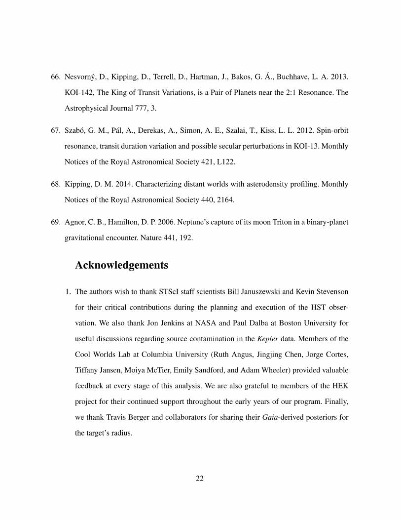
Acknowledgements

1. The authors wish to thank STScI staff scientists Bill Januszewski and Kevin Stevenson

for their critical contributions during the planning and execution of the HST obser-

vation. We also thank Jon Jenkins at NASA and Paul Dalba at Boston University for

useful discussions regarding source contamination in the Kepler data. Members of the

Cool Worlds Lab at Columbia University (Ruth Angus, Jingjing Chen, Jorge Cortes,

Tiffany Jansen, Moiya McTier, Emily Sandford, and Adam Wheeler) provided valuable

feedback at every stage of this analysis. We are also grateful to members of the HEK

project for their continued support throughout the early years of our program. Finally,

we thank Travis Berger and collaborators for sharing their Gaia-derived posteriors for

the target’s radius.

22

1. Funding and Support: Analysis was carried out in part on the NASA Supercomputer

PLEIADES (Grant #HEC-SMD-17-1386). AT is supported through the NSF Graduate

Research Fellowship (DGE 16-44869). DK is supported by the Alfed P. Sloan Founda-

tion Fellowship. This work is based in part on observations made with the NASA/ESA

Hubble Space Telescope, obtained at the Space Telescope Science Institute, which is op-

erated by the Association of Universities for Research in Astronomy, Inc., under NASA

contract NAS 5-26555. These observations are associated with program #GO-15149.

Support for program #GO-15149 was provided by NASA through a grant from the

Space Telescope Science Institute, which is operated by the Association of Universi-

ties for Research in Astronomy, Inc., under NASA contract NAS 5-26555. This paper

includes data collected by the Kepler Mission. Funding for the Kepler Mission is pro-

vided by the NASA Science Mission directorate. This research has made use of the

Exoplanet Follow-up Observation Program website, which is operated by the Califor-

nia Institute of Technology, under contract with the National Aeronautics and Space

Administration under the Exoplanet Exploration Program.

1. Software This work made use of Numpy, Scipy, Pandas, Matplotlib, Astropy,

TTVfaster, Exo-Transmit, forecaster, LUNA and MULTINEST.

List of Supplementary Materials

1. Materials and Methods

2. Tables S1-S4

3. Figures S1-S12

4. References (42-69)

23

Table 1: Bayesian evidences (Z) and maximum likelihoods (L) from our combined fits usingKepler and new HST data. Kepler+HST fits. The subscripts are P for planet model, T for plan-etary TTV model, Z for a zero-radius moon model and M for moon model. The three columnsare for each trend model attempted.

linear quadratic exponentiallogZP 6302.79± 0.11 6306.68± 0.11 6308.41± 0.11logZT 6304.86± 0.11 6308.81± 0.12 6305.11± 0.11logZZ 6306.84± 0.11 6311.12± 0.12 6310.82± 0.12logZM 6315.73± 0.12 6312.92± 0.12 6314.01± 0.12

2 logK(Z ′M/Z ′P) 1.00± 0.222 log(ZM/ZP) 25.88± 0.32 12.47± 0.33 11.19± 0.322 log(ZM/ZT) 21.72± 0.33 8.21± 0.34 17.81± 0.332 log(ZM/ZZ) 17.77± 0.33 3.61± 0.33 6.38± 0.34

∆χ′2PM = 2 log(L′M/L′P) 18.66

∆χ2PM = 2 log(LM/LP) 54.93 41.04 41.57

∆χ2TM = 2 log(LM/LT) 35.69 23.97 38.71

∆χ2ZM = 2 log(LM/LZ) 33.68 19.59 19.22

24

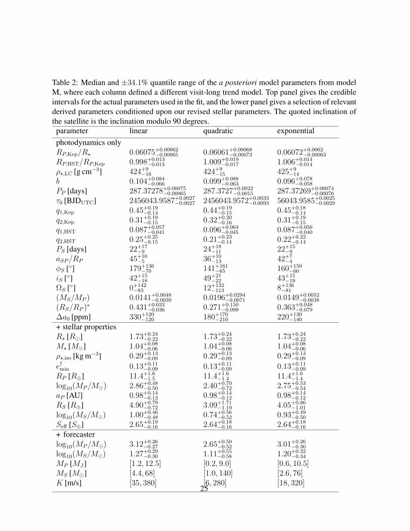
Table 2: Median and ±34.1% quantile range of the a posteriori model parameters from modelM, where each column defined a different visit-long trend model. Top panel gives the credibleintervals for the actual parameters used in the fit, and the lower panel gives a selection of relevantderived parameters conditioned upon our revised stellar parameters. The quoted inclination ofthe satellite is the inclination modulo 90 degrees.

parameter linear quadratic exponentialphotodynamics onlyRP,Kep/R? 0.06075+0.00062

−0.00065 0.06061+0.00068−0.00073 0.06072+0.0062

−0.00063

RP,HST/RP,Kep 0.998+0.013−0.013 1.009+0.019

−0.017 1.006+0.014−0.014

ρ?,LC [g cm−3] 424+9−16 424+9

−15 425+9−14

b 0.104+0.084−0.066 0.099+0.088

−0.063 0.096+0.078−0.058

PP [days] 287.37278+0.00075−0.00065 287.3727+0.0022

−0.0015 287.37269+0.00074−0.00076

τ0 [BJDUTC] 2456043.9587+0.0027−0.0027 2456043.9572+0.0033

−0.0093 56043.9585+0.0025−0.0029

q1,Kep 0.45+0.19−0.14 0.44+0.19

−0.15 0.45+0.18−0.14

q2,Kep 0.31+0.19−0.15 0.32+0.20

−0.16 0.31+0.19−0.15

q1,HST 0.087+0.057−0.041 0.096+0.064

−0.045 0.087+0.056−0.040

q2,HST 0.25+0.25−0.15 0.21+0.23

−0.14 0.22+0.22−0.14

PS [days] 22+17−9 24+18

−11 22+15−9

aSP/RP 45+10−5 36+10

−13 42+7−4

φS [] 179+136−70 141+161

−65 160+150−60

iS [] 42+15−18 49+21

−22 43+15−19

ΩS [] 0+142−83 12+132

−113 8+136−81

(MS/MP ) 0.0141+0.0048−0.0039 0.0196+0.0294

−0.0071 0.0149+0.0052−0.0038

(RS/RP )∗ 0.431+0.033−0.036 0.271+0.150

−0.099 0.363+0.048−0.079

∆a0 [ppm] 330+120−120 180+170

−210 220+130−140

+ stellar propertiesR? [R] 1.73+0.24

−0.22 1.73+0.24−0.22 1.73+0.24

−0.22

M? [M] 1.04+0.08−0.06 1.04+0.08

−0.06 1.04+0.08−0.06

ρ?,iso [kg m−3] 0.29+0.13−0.09 0.29+0.13

−0.09 0.29+0.13−0.09

e†min 0.13+0.11−0.09 0.13+0.11

−0.09 0.13+0.11−0.09

RP [R⊕] 11.4+1.6−1.5 11.4+1.6

−1.4 11.4+1.6−1.4

log10(MP/M) 2.86+0.48−0.50 2.40+0.70

−0.72 2.75+0.53−0.54

aP [AU] 0.98+0.14−0.13 0.98+0.14

−0.12 0.98+0.14−0.12

RS [R⊕] 4.90+0.79−0.72 3.09+1.71

−1.19 4.05+0.86−1.01

log10(MS/M) 1.00+0.46−0.48 0.74+0.56

−0.52 0.93+0.49−0.50

Seff [S⊕] 2.65+0.19−0.16 2.64+0.18

−0.16 2.64+0.18−0.16

+ forecasterlog10(MP/M) 3.12+0.26

−0.27 2.65+0.50−0.52 3.01+0.26

−0.30

log10(MS/M) 1.27+0.29−0.30 1.11+0.55

−0.58 1.20+0.32−0.34

MP [MJ ] [1.2, 12.5] [0.2, 9.0] [0.6, 10.5]MS [M] [4.4, 68] [1.0, 140] [2.6, 76]K [m/s] [35, 380] [6, 280] [18, 320]

25

Figure 1: Comparison of five different methods used for detrending the SAP Kepler data. Base-lines shown represent the full training set used, except for the local method which is trainedon only data immediately surrounding the transits of interest.

26

[ - ]

18300

18250

18200

18150

[ - ]

[ - ]

18300

18250

18200

18150

[ - ]

[ - ]

18300

18250

18200

[ - ]

18150

intra-orbit RMS = 544.8 ppm

intra-orbit RMS = 477.3 ppm

KIC 4760469KIC 4760478

uncorrecteduncorrected

exponential ramp model exponential ramp model

non-parametric correction non-parametric correction

intra-orbit RMS =440.1 ppm

intra-orbit RMS = 375.5 ppm

countscounts

counts

Figure 2: Top row shows the optimal aperture photometry of our target (left) and the bestcomparison star (right), where the hooks and visit-long trends are clearly present. Points arecolored by their exposure number within each HST orbit (triangles represent outliers). Middlerow shows a hook-correction using the common exponential ramp model on both stars. Bottomrow shows the result from an alternative and novel hook-correction approach introduced in thiswork.

27

2logKMZ = 6.38logKM = 6314.01

2logKMZ = 17.77 logKM = 6315.73

2logKMZ = 3.61 logKM = 6312.92

linear

quadratic

exponential

Figure 3: The HST observations with three proposed trends fit to the data (left) and with thetrends removed (right). Bottom-right numbers in each row give the Bayes factor between aplanet+moon model (model M) and a planet+moon model where the moon radius equals zero(model Z), which tracks the significance of the moon-like dip in isolation.

28

3055.0 3055.5 3056.0 3056.5-6

-5

-4

-4

-2

-1

0

+1

BJD-2,455,400

relativeintensity[ppt]

3055.0 3055.5 3056.0 3056.5-6

-5

-4

-4

-2

-1

0

+1

BJD-2,455,400

relativeintensity[ppt]

-7

-6

-5

-4

-4

-2

-1

0

+1

+2

+31330.0 1330.5 1331.0 1331.5 1332.0 1332.5

relativeintensity[ppt]

BJD-2,455,400

-7

-6

-5

-4

-4

-2

-1

0

+1

+2

+31042.5 1043.0 1043.5 1044.0 1044.5 1045.0 1045.5

relativeintensity[ppt]

BJD-2,455,400

-7

-6

-5

-4

-4

-2

-1

0

+1

+2

+3468.0 468.5 469.0 469.5 470.0 470.5

relativeintensity[ppt]

BJD-2,455,400

3055.0 3055.5 3056.0 3056.5-6

-5

-4

-4

-2

-1

0

+1

BJD-2,455,400

relativeintensity[ppt]

linear quadratic exponential

epoch -2 (Kepler) epoch 0 (Kepler) epoch +1 (Kepler)

epoch +7 (HST) epoch +7 (HST) epoch +7 (HST)

BJD - 2,455,400

Figure 4: The three transits in Kepler (top) and the October 2017 transit observed with HST(bottom) for three three trend model solutions. The three colored lines show the three corre-sponding trend model solutions for model M, our favored transit model. The shape of the HSTtransit differs from the Kepler transits due to limb darkening differences between the band-passes.

29