arX

iv:a

stro

-ph/

0703

429v

1 1

6 M

ar 2

007

The Cosmic Coincidence as a Temporal Selection Effect Produced

by the Age Distribution of Terrestrial Planets in the Universe

Charles H. Lineweaver1 & Chas A. Egan1,2

1 Planetary Science Institute, Research School of Astronomy and Astrophysics &

Research School of Earth Sciences, Australian National University, Canberra, ACT,

Australia

2 Department of Astrophysics, School of Physics, University of New South Wales,

Sydney, NSW 2052, Australia

charley@mso.anu.edu.au

ABSTRACT

The energy densities of matter and the vacuum are currently observed to be

of the same order of magnitude: (Ωmo≈ 0.3) ∼ (ΩΛo

≈ 0.7). The cosmological

window of time during which this occurs is relatively narrow. Thus, we are

presented with the cosmological coincidence problem: Why, just now, do these

energy densities happen to be of the same order? Here we show that this apparent

coincidence can be explained as a temporal selection effect produced by the age

distribution of terrestrial planets in the Universe. We find a large ( ∼ 68%)

probability that observations made from terrestrial planets will result in finding

Ωm at least as close to ΩΛ as we observe today. Hence, we, and any observers in

the Universe who have evolved on terrestrial planets, should not be surprised to

find Ωmo∼ ΩΛo

. This result is relatively robust if the time it takes an observer

to evolve on a terrestrial planet is less than ∼ 10 Gyr.

Subject headings: Terrestrial Planets, Cosmology, Planets, Cosmic Coincidence

1. Is the Cosmic Coincidence Remarkable or Insignificant?

1.1. Dicke’s argument

Dirac (1937) pointed out the near equality of several large fundamental dimensionless

numbers of the order 1040. One of these large numbers varied with time since it depended on

the age of the Universe. Thus there was a limited time during which this near equality would

hold. Under the assumption that observers could exist at any time during the history of the

– 2 –

Universe, this large number coincidence could not be explained in the standard cosmology.

This problem motivated Dirac (1938) and Jordan (1955) to construct an ad hoc new cosmol-

ogy. Alternatively, Dicke (1961) proposed that our observations of the Universe could only

be made during a time interval after carbon had been produced in the Universe and before

the last stars stop shining. Dicke concluded that this temporal observational selection effect

– even one so loosely delimited – could explain Dirac’s large number coincidence without

invoking a new cosmology.

Here, we construct a similar argument to address the cosmic coincidence: Why just now

do we find ourselves in the relatively brief interval during which Ωm ∼ ΩΛ. The temporal

constraints on observers that we present are more empirical and specific than those used

in Dicke’s analysis, but the reasoning is similar. Our conclusion is also similar: a temporal

observational selection effect can explain the apparent cosmic coincidence. That is, given the

evolution of ΩΛ and Ωm in our Universe, most observers in our Universe who have emerged

on terrestrial planets will find ΩΛ ∼ Ωm. Rather than being an unusual coincidence, it is

what one should expect.

There are two distinct problems associated with the cosmological constant (Weinberg

2000; Garriga and Vilenkin 2001; Steinhardt 2003). One is the coincidence problem that

we address here. The other is the smallness problem and has to do with the observed en-

ergy density of the vacuum, ρΛ. Why is ρΛ so small compared to the ∼ 10120 times larger

value predicted by particle physics? Anthropic solutions to this problem invoke a multi-

verse and argue that galaxies would not form and there would be no life in a Universe,

if ρΛ were larger than ∼ 100 times its observed value (Weinberg 1987; Martel et al. 1998;

Garriga and Vilenkin 2001; Pogosian and Vilenkin 2007). Such explanations for the small-

ness of ρΛ do not explain the temporal coincidence between the time of our observation and

the time of the near-equality of Ωm and ΩΛ. Here we address this temporal coincidence in

our Universe, not the smallness problem in a multiverse.

1.2. Evolution of the Energy Densities

Given the currently observed values for Ho and the energy densities Ωro, Ωmo

and ΩΛo

in the Universe (Spergel et al. 2006; Seljak et al. 2006), the Friedmann equation tells us the

evolution of the scale factor a, and the evolution of these energy densities. These are plotted

in Fig. 1. The history of the Universe can be divided chronologically into four distinct periods

each dominated by a different form of energy: initially the false vacuum energy of inflation

dominates, then radiation, then matter, and finally vacuum energy. Currently the Universe

is making the transition from matter domination to vacuum energy domination. In an ex-

– 3 –

Fig. 1.— The time dependence of the densities of the major components of the Universe.

Given the observed Hubble constant, Ho and energy densities in the Universe today, Ωro,

Ωmo, ΩΛo

(radiation, matter and cosmological constant), we use the Friedmann equation

to plot the temporal evolution of the components of the Universe in g/cm3 (top panel), or

normalized to the time-dependent critical density ρcrit = 3H(t)2

8πG(bottom panel). We assume

an epoch of inflation at ∼ 10−35 seconds after the big bang and a false vacuum energy density

ρΛinfbetween the Planck scale and tGUT . See Table 1 and Appendix A for details.

– 4 –

panding Universe, with an initial condition Ωm > ΩΛ > 0, there will be some epoch in which

Ωm ∼ ΩΛ, since ρm is decreasing as ∝ 1/a3 while ρΛ is a constant (see top panel of Fig. 1 and

Appendix A). Figure 1 also shows that the transition from matter domination to vacuum

energy domination is occurring now. When we view this transition in the context of the time

evolution of the Universe (Fig. 2) we are presented with the cosmic coincidence problem:

Why just now do we find ourselves at the relatively brief interval during which this transition

happens? Carroll (2001b,a) and Dodelson et al. (2000) find this coincidence to be a remark-

able result that is crucial to understand. The cosmic coincidence problem is often regarded

as an important unsolved problem whose solution may help unravel the nature of dark energy

(Turner 2001; Carroll 2001a). The coincidence problem is one of the main motivations for

the tracker potentials of quintessence models (Caldwell et al. 1998; Steinhardt et al. 1999;

Zlatev et al. 1999; Wang et al. 2000; Dodelson et al. 2000; Armendariz-Picon et al. 2000;

Guo and Zhang 2005). In these models the cosmological constant is replaced by a more

generic form of dark energy in which Ωm and ΩΛ are in near-equality for extended peri-

ods of time. It is not clear that these models successfully explain the coincidence without

fine-tuning (see Weinberg 2000; Bludman 2004).

The interpretation of the observation Ωmo∼ ΩΛo

as a remarkable coincidence in need

of explanation depends on some assumptions that we quantify to determine how surprising

this apparent coincidence is. We begin this quantification by introducing a time-dependent

proximity parameter,

r = min

[

ΩΛ

Ωm

,Ωm

ΩΛ

]

(1)

which is equal to one when Ωm = ΩΛ and is close to zero when Ωm >> ΩΛ or Ωm << ΩΛ.

The current value is ro ≈ 0.4. In Figure 2 we plot r as a function of log(scale factor) in

the upper panel and as a function of log(time) in the lower panel. These logarithmic axes

allow a large dynamic range that makes our existence at a time when r ∼ 1, appear to be

an unlikely coincidence. This appearance depends on the implicit assumption that we could

make cosmological observations at any time with equal likelihood. More specifically, the

implicit assumption is that the a priori probability distribution Pobs, of the times we could

have made our observations, is uniform in log t, or log a, over the interval shown.

Our ability to quantify the significance of the coincidence depends on whether we assume

that Pobs is uniform in time, log(time), scale factor or log(scale factor). That is, our result de-

pends on whether we assume: Pobs(t) = constant, Pobs(log t) = constant, Pobs(a) = constant

or Pobs(log a) = constant. These are the most common possibilities, but there are others.

For a discussion of the relative merits of log and linear time scales and implicit uniform

priors see Section 3.3 and Jaynes (1968).

In Fig. 3 we plot r(t) on an axis linear in time where the implicit assumption is that the

– 5 –

a priori probability distribution of our existence is uniform in t over the intervals [0, 100] Gyr

(top panel) and [0, 13.8] Gyr (bottom panel). The bottom panel shows that the observation

r > 0.4 could have been made anytime during the past 7.8 Gyr. Thus, our current observation

that ro ≈ 0.4, does not appear to be a remarkable coincidence. Whether this most recent

7.8 Gyr period is seen as “brief” (in which case there is an unlikely coincidence in need of

explanation) or “long” (in which case there is no coincidence to explain) depends on whether

we view the issue in log time (Fig. 2) or linear time (Fig. 3).

A large dynamic range is necessary to present the fundamental changes that occurred

in the very early Universe, e.g., the transitions at the Planck time, inflation, baryogenesis,

nucleosynthesis, recombination and the formation of the first stars. Thus a logarithmic

time axis is often preferred by early Universe cosmologists because it seems obvious, from

the point of view of fundamental physics, that the cosmological clock ticks logarithmically.

This defensible view and the associated logarithmic axis gives the impression that there is

a coincidence in need of an explanation. The linear time axis gives a somewhat different

impression. Evidently, deciding whether a coincidence is of some significance or only an

accident is not easy (Peebles 1999). We conclude that although the importance of the

cosmic coincidence problem is subjective, it is important enough to merit the analysis we

perform here.

The interpretation of the observation Ωmo∼ ΩΛo

as a coincidence in need of explanation

depends on the a priori (not necessarily uniform) probability distribution of our existence.

That is, it depends on when cosmological observers can exist. We propose that the cosmic

coincidence problem can be more constructively evaluated by replacing these uninformed

uniform priors with the more realistic assumption that observers capable of measuring cos-

mological parameters are dependent on the emergence of high density regions of the Universe

called terrestrial planets, which require non-trivial amounts of time to form – and that once

these planets are in place, the observers themselves require non-trivial amounts of time to

evolve.

In this paper we use the age distribution of terrestrial planets estimated by Lineweaver

(2001) to constrain when in the history of the Universe, observers on terrestrial planets can

exist. In Section 2, we briefly describe this age distribution (Fig. 4) and show how it limits

the existence of such observers to an interval in which Ωm ∼ ΩΛ (Fig. 5). Using this age

distribution as a temporal selection function, we compute the probability of an observer

on a terrestrial planet observing r ≥ ro (Fig. 6). In Section 3 we discuss the robustness

of our result and find (Fig. 7) that this result is relatively robust if the time it takes an

observer to evolve on a terrestrial planet is less than ∼ 10 Gyr. In Section 4 we discuss and

summarize our results, and compare it to previous work to resolve the cosmic coincidence

– 6 –

Fig. 2.— Plot of the proximity factor r (see Eq. 1). When the matter and vacuum energy

densities of the Universe are the same, Ωm = ΩΛ, we have r = 1. We currently observe

Ωmo∼ ΩΛo

and thus, r ∼ 1. Our existence now when r ∼ 1 appears to be an unlikely cosmic

coincidence when the x axis is logarithmic in the scale factor (top panel) or logarithmic in

time (bottom panel). In the top panel, following Carroll (2001b), we have chosen a range

of scale factors with “Now” midway between the scale factor at the Planck time and the

scale factor at the inverse Planck time [aP lanck < a < a−1P lanck]. The brief epoch shown

in grey between the thin vertical lines is the epoch during which r > ro (where ro ≈ 0.4

is the currently observed value). In the bottom panel the range shown on the x axis is

[tP lanck < t < 1022] seconds. The Planck time and Planck scale provide reasonably objective

lower time limits. The upper limits are somewhat arbitrary but contribute to the impression

that r ≈ 0.4 ∼ 1 is an unlikely coincidence.

– 7 –

Fig. 3.— Plot of the proximity factor r, as in the previous figure, but plotted here with

a linear rather than a logarithmic time axis. The condition r > ro ≈ 0.4 does not seem as

unlikely as in the previous figure. The range of time plotted also affects this appearance;

with the [0, 100] Gyr range of the top panel, the time interval highlighted in grey where

r > ro, appears narrow and relatively unlikely. In contrast, the [0, 13.8] Gyr range of the

bottom panel seems to remove the appearance of r > ro being an unlikely coincidence in

need of explanation; for the first ∼ 6 Gyrs we have r < ro while in the subsequent 7.8 Gyr

we have r > ro. How can r > ro be an unlikely coincidence when it has been true for most

of the history of the Universe?

– 8 –

problem (Garriga et al. 2000; Bludman and Roos 2001).

2. How We Compute the Probability of Observing Ωm ∼ ΩΛ

2.1. The Age Distribution of Terrestrial Planets and New Observers

The mass histogram of detected extrasolar planets peaks at low masses: dN/dM ∝

M−1.7, suggesting that low mass planets are abundant (Lineweaver and Grether 2003). Ter-

restrial planet formation may be a common feature of star formation (Wetherill 1996; Chyba

1999; Ida and Lin 2005). Whether terrestrial planets are common or rare, they will have an

age distribution proportional to the star formation rate – modified by the fact that in the

first ∼ 2 billion years of star formation, metallicities are so low that the material for terres-

trial planet formation will not be readily available. Using these considerations, Lineweaver

(2001) estimated the age distribution of terrestrial planets – how many Earths are produced

by the Universe per year, per Mpc3 (Figure 4). If life emerges rapidly on terrestrial planets

(Lineweaver and Davis 2002) then this age distribution is the age distribution of biogenesis

in the Universe. However, we are not just interested in any life; we would like to know the

distribution in time of when independent observers first emerge and are able to measure Ωm

and ΩΛ, as we are able to do now. If life originates and evolves preferentially on terrestrial

planets, then the Lineweaver (2001) estimate of the age distribution of terrestrial planets is

an a priori input which can guide our expectations of when we (as members of a hypothet-

ical group of terrestrial-planet-bound observers) could have been present in the Universe.

It takes time (if it happens at all) for life to emerge on a new terrestrial planet and evolve

into cosmologists who can observe Ωm and ΩΛ. Therefore, to obtain the age distribution

of new independent observers able to measure the composition of the Universe for the first

time, we need to shift the age distribution of terrestrial planets by some characteristic time,

∆tobs required for observers to evolve. On Earth, it took ∆tobs ∼ 4 Gyr for this to happen.

Whether this is characteristic of life elsewhere in the Universe is uncertain (Carter 1983;

Lineweaver and Davis 2003). For our initial analysis we use ∆tobs = 4 Gyr as a nominal

time to evolve observers. In Section 3.1 we allow ∆tobs to vary from 0-12 Gyr to see how

sensitive our result is to these variations. Fig. 4 shows the age distribution of terrestrial

planet formation in the Universe shifted by ∆tobs = 4 Gyr. This curve, labeled “Pobs” is a

crude prior for the temporal selection effect of when independent observers can first measure

r. Thus, if the evolution of biological equipment capable of doing cosmology takes about

∆tobs ∼ 4 Gyr, the “Pobs” in Fig. 4 shows the age distribution of the first cosmologists on

terrestrial planets able to look at the Universe and determine the overall energy budget, just

as we have recently been able to do.

– 9 –

Fig. 4.— The terrestrial planet formation rate PFR(t), derived in Lineweaver (2001) is an

estimate of the age distribution of terrestrial planets in the Universe and is shown here as

a thin solid line. Estimated uncertainty is given by the thin dashed lines. To allow time

for the evolution of observers on terrestrial planets, we shift this distribution by ∆tobs to

obtain an estimate of the age distribution of observers: Pobs(t) = PFR(t − ∆tobs) (thick

solid line). The grey band represents the error estimate on Pobs(t) which is the shifted error

estimates on PFR(t). In the case shown here ∆tobs = 4 Gyr, which is how long it took life

on Earth to emerge, evolve and be able to measure the composition of the Universe. To

obtain the numerical values on the y axis, we have followed Lineweaver (2001) and assumed

that one out of one hundred stars is orbited by a terrestrial planet. We have smoothly

extrapolated the PFR(t) of Lineweaver (2001) into the future. This time dependence and

our subsequent analysis does not depend on whether the probability for terrestrial planets

to produce observers is high or low.

– 10 –

Fig. 5.— Zoom-in of the portion of Fig. 1 between 1 and 100 billion years after the big

bang, containing the relatively narrow window of time in which Ωm ∼ ΩΛ. The 99 Gyr time

interval displayed here is indicated in Fig. 1 by the small grey rectangle above the “Now”

label. The proximity parameter r(t) (Eq. 1, Figs. 2 & 3) is superimposed. The thin solid

line shows the age distribution of terrestrial planets in the Universe while the thick solid line

is the lateral displacement of this distribution by ∆tobs = 4 Gyr. These distributions were

presented in Fig. 4, but here the time axis is logarithmic. We interpret Pobs as the frequency

distribution of new observers able to measure Ωm and ΩΛ for the first time. Since r(t) peaks

at about the same time as Pobs(t), large values of r will be observed more often than small

values.

– 11 –

2.2. The Probability of Observing Ωm ∼ ΩΛ.

In Fig. 5 we zoom into the portion of Fig. 1 containing the relatively narrow window

of time in which Ωm ∼ ΩΛ. We plot r(t) to show where r ∼ 1 and we also plot the age

distribution of planets and the age distribution of recently emerged cosmologists from Fig.

4. The white area under the thick Pobs(t) curve provides an estimate of the time distribution

of new observers in the Universe. We interpret Pobs(t) as the probability distribution of the

times at which new, independent observers are able to measure r for the first time.

Lineweaver (2001) estimated that the Earth is relatively young compared to other ter-

restrial planets in the Universe. It follows under the simple assumptions of our analysis that

most terrestrial-planet-bound observers will emerge earlier than we have. We compute the

fraction f of observers who have emerged earlier than we have,

f =

∫ to

0Pobs(t) dt

∫

∞

0Pobs(t) dt

≈ 68% (2)

and find that 68% emerge earlier while 32% emerge later. These numbers are indicated in

Fig. 5.

2.3. Converting Pobs(t) to Pobs(r)

We have an estimate of the distribution in time of observers, Pobs(t), and we have the

proximity parameter r(t). We can then convert these to a probability Pobs(r), of observed

values of r. That is, we change variables and convert the t−dependent probability to an

r−dependent probability: Pobs(t) → Pobs(r). We want the probability distribution of the r

values first observed by new observers in the Universe. Let the probability of observing r in

the interval dr be Pobs(r)dr. This is equal to the probability of observing t in the interval

dt, which is Pobs(t)dt

Thus,

Pobs(r) dr = Pobs(t) dt (3)

or equivalently

Pobs(r) =Pobs(t)

dr/dt(4)

where Pobs(t) = PFR(t − ∆tobs) is the temporally shifted age distribution of terrestrial

planets and dr/dt is the slope of r(t). Both are shown in Fig. 5. The distribution Pobs(r)

is shown in Fig. 6 along with the upper and lower confidence limits on Pobs(r) obtained by

– 12 –

inserting the upper and lower confidence limits of Pobs(t) (denoted “P+” and “P−” in Fig.

4), into Eq. 4 in place of Pobs(t).

The probability of observing r > ro is,

P (r > ro) =

∫ 1

ro

Pobs(r) dr =

∫ to

t′Pobs(t) dt ≈ 68% (5)

where t′ is the time in the past when r was equal to its present value, i.e., r(t′) = r(to) =

ro ≈ 0.4. We have t′ = 6 Gyr and to = 13.8 Gyr (see bottom panel of Fig. 3). This

integral is shown graphically in Fig. 6 as the hatched area underneath the “Pobs(r)” curve,

between r = ro and r = 1. We interpret this as follows: of all observers that have emerged

on terrestrial planets, 68% will emerge when r > ro and thus will find r > ro. The 68% from

Eq. 2 is only the same as the 68% from Eq. 5 because all observers who emerge earlier than

we did, did so more recently than 7.8 billion years ago and thus, observe r > ro (Fig. 5).

Fig. 6.— Probability of new observers on terrestrial planets observing a given r (Eq. 4).

Given our estimate of the age distribution of new cosmologists in the Universe Pobs(t), the

probability of observing Ωm and ΩΛ as close together as they are, or closer, is the integral

given in Eq. (5), shown here as the hashed area labeled 68%. The dashed lines labeled P+

and P− are from replacing Pobs(t) in Eq. 4 with the curves labeled P+ and P− in Fig. 4.

We obtain estimates of the uncertainty on this 68% estimate by computing analogous

– 13 –

integrals underneath the curves labeled P+ and P− in Fig. 6. These yield 82% and 59%

respectively. Thus, under the assumptions made here, 68+14−10% of the observers in the Universe

will find ΩΛ and Ωm even closer to each other than we do. This suggests that a temporal

selection effect due to the constraints on the emergence of observers on terrestrial planets

provides a plausible solution to the cosmic coincidence problem. If observers in our Universe

evolve predominantly on Earth-like planets (see the “principle of mediocrity” in Vilenkin

(1995b)), we should not be surprised to find ourselves on an Earth-like planet and we should

not be surprised to find ΩΛo∼ Ωmo

.

3. How Robust is this 68% Result?

3.1. Dependence on the timescale for the evolution of observers

A necessary delay, required for the biological evolution of observing equipment – e.g.

brains, eyes, telescopes, makes the observation of recent biogenesis unobservable (Lineweaver and Davis

2002, 2003). That is, no observer in the Universe can wake up to observerhood and find that

their planet is only a few hours old. Thus, the timescale for the evolution of observers,

∆tobs > 0.

Our 68+14−10% result was calculated under the assumption that evolution from a new

terrestrial planet to an observer takes ∆tobs ∼ 4 Gyr. To determine how robust our result

is to variations in ∆tobs, we perform the analysis of Sec. 2 for 0 < ∆tobs < 12 Gyr. The

results are shown in Fig. 7. Our 68+14−10% result is the data point plotted at ∆tobs = 4

Gyr. If life takes ∼ 0 Gyr to evolve to observerhood, once a terrestrial planet is in place,

Pobs(t) ≈ PFR(t) and 55% of new cosmologists would observe an r value larger than the

ro ≈ 0.4 that we actually observe today. If observers typically take twice as long as we did

to evolve (∆tobs ∼ 8 Gyr), there is still a large chance (∼ 30%) of observing r > ro. If

∆tobs > 11 Gyr, Pobs(t) in Fig. 5 peaks substantially after r(t) peaks, and the percentage

of cosmologists who see r > ro, is close to zero (Eq. 5). Thus, if the characteristic time it

takes for life to emerge and evolve into cosmologists is ∆tobs<∼ 10 Gyr, our analysis provides

a plausible solution to the cosmic coincidence problem.

The Sun is more massive than 94% of all stars. Therefore 94% of stars live longer than

the t⊙ ≈ 10 Gyr main sequence lifetime of the Sun. This is mildly anomalous and it is

plausible that the Sun’s mass has been anthropically selected. For example, perhaps stars

as massive as the Sun are needed to provide the UV photons to jump start and energize the

molecular evolution that leads to life. If so, then ∼ 10 Gyr is a rough upper limit to the

amount of time a terrestrial planet with simple life has to produce observers. Even if the

– 14 –

characteristic time for life to evolve into observers is much longer than 10 Gyr, as concluded

by Carter (1983), this UV requirement that life-hosting stars have main sequence lifetimes<∼ 10 Gyr would lead to the extinction of most extraterrestrial life before it can evolve into

observers. This would lead to observers waking to observerhood to find the age of their

planet to be a large fraction of the main sequence lifetime of their star; the time they took

to evolve would satisfy ∆tobs<∼ 10 Gyr, and they would observe that r ∼ 1 and that other

observers are very rare. Such is our situation.

If we assume that we are typical observers (Vilenkin 1995a,b, 1996a,b) and that the

coincidence problem must be resolved by an observer selection effect (Bostrom 2002), then

we can conclude that the typical time it takes observers to evolve on terrestrial planets is

less than 10 Gyr (∆tobs < 10 Gyr).

3.2. Dependence on the age distribution of terrestrial planets

The Pobs(t) used here (Fig. 5) is based on the star formation rate (SFR) computed

in Lineweaver (2001). There is general agreement that the SFR has been declining since

redshifts z ∼ 2. Current debate centers around whether that decline has only been since z ∼

2 or whether the SFR has been declining from a much higher redshift (Lanzetta et al. 2002;

Hopkins and Beacom 2006; Nagamine et al. 2006; Thompson et al. 2006). Since Lineweaver

(2001) assumed a relatively high value for the SFR at redshifts above 2, this led to a relatively

high estimate of the metallicity of the Universe at z ∼ 2, which corresponds to a relatively

short delay (∼ 2 Gyr) between the big bang and the first terrestrial planets. For the purposes

of this analysis, the early-SFR-dependent uncertainty in the ∼ 2 Gyr delay is degenerate

with, but much smaller than, the uncertainty of ∆tobs. Thus the variations of ∆tobs discussed

above subsume the SFR-dependent uncertainty in Pobs(t).

3.3. Dependence on Measure

In Figs. 2 & 3 we illustrated how the importance of the cosmic coincidence depends

on the range over which one assumes that the observation of r could have occurred. This

involved choosing the range ∆x shown on the x axis in Figs. 2 & 3. We also showed how

the apparent significance of the coincidence depended on how one expressed that range, i.e.,

logarithmic in Fig. 2 and linear in Fig. 3. The coincidence seems most compelling when ∆x

is the largest and the problem is presented on a logarithmic x axis. This dependence is a

specific example of a “measure” problem (Aguirre and Tegmark 2005; Aguirre et al. 2006).

– 15 –

Fig. 7.— Percentage of cosmologists who see r > ro as a function of the time ∆tobs, it takes

observers to evolve on a terrestrial planet. Since we have only vague notions about how long

it takes observers to evolve on a planet, we vary ∆tobs between 0 and 12 billion years and

show how the probability P (r > ro) of observing r > ro (Eq. 5) varies as a function of ∆tobs.

The 68+14−10% point plotted is the result from Fig. 6 where ∆tobs = 4 Gyr. If ∆tobs = 0, we

use the thin solid line in Fig. 5 as Pobs(t) rather than the thick solid line and we obtain 55%.

– 16 –

The measure problem is illustrated in Fig. 8, where we plot four different uniform

distributions of observers on a linear time axis. In Panel a) Pobs(t) = constant. That is, we

assume that observers could find themselves anywhere between trec = 380, 000 yr and 100

Gyr after the big bang, with uniform probability (dark grey). In b), we make the different

assumption that observers are distributed uniformly in log(t) over the same range in time.

This means for example that the probability of finding yourself between 0.1 and 1 Gyr is the

same as between 1 and 10 Gyr. We plot this as a function of linear time and find that the

distribution of observers (dark grey) is highest towards earlier times.

To quantify and explore these dependencies further, in Table 2, we take the duration

when r > ro (call this interval ∆xr) and divide it by various larger ranges ∆x (a range of

Fig. 8.— The expected observed value of r depends strongly on the assumed distribution of

observers over time t. This figure demonstrates a variety of uniform observer distributions

Pobs which, if used, result in the cosmic coincidence problem that the observed value of r is

unexpectedly high. The Pobs that are functions of log(a) or log(t) have been normalized to

the interval trec to 100 Gyr. Panel a) is the same as the top panel of Fig. 3. The probabilities

that an observer would fall within the vertical light grey band (r > ro) in Panels a,b,c and

d are 8%, 7%, 0.2% and 6% respectively, and are given in the first row of Table 2.

– 17 –

time or scale factor). Thus, when the probability P (r > ro) = ∆xr

∆xis << 1, there is a low

probability that one would find oneself in the interval ∆xr and the cosmic coincidence is

compelling. However, when P (r > ro) ∼ 1 the coincidence is not significant.

In the four panels a,b,c and d of Fig. 8 the probability of us observing r ≥ ro (finding

ourselves in the light grey area) is respectively 8%, 7%, 0.2% and 6%. These values are given

in the first row of Table 2 along with analogous values when 11 other ranges for ∆x are

considered. Probabilities corresponding to the four panels of Figs. 2 & 3 are shown in bold

in Table 2. Our conclusion is that this simple ratio method of measuring the significance of a

coincidence yields results that can vary by many orders of magnitude depending on the range

(∆x) and measure (e.g. linear or logarithmic) chosen. The use of the non-uniform Pobs(t)

shown in Fig. 4 is not subject to these ambiguities in the choice of range and measure.

4. Discussion & Summary

Anthropic arguments to resolve the coincidence problem include Garriga et al. (2000)

and Bludman and Roos (2001). Both use a semi-analytical formalism (Gunn and Gott 1972;

Press and Schechter 1974; Martel et al. 1998) to compute the number density of objects that

collapse into large galaxies. This is then used as a measure of the number density of intelligent

observers. Our work complements these semi-analytic models by using observations of the

star formation rate to constrain the possible times of observation. Our work also extends

this previous work by including the effect of ∆tobs, the time it takes observers to evolve

on terrestrial planets. This inclusion puts an important limit on the validity of anthropic

solutions to the coincidence problem.

Garriga et al. (2000) is probably the work most similar to ours. They take ρΛ as a

random variable in a multiverse model with a prior probability distribution. For a wide

range of ρΛ (prescribed by a prior based on inflation theory) they find approximate equality

between the time of galaxy formation tG, the time when Λ starts to dominate the energy

density of the Universe tΛ and now to. That is, they find that, within one order of magnitude,

tG ∼ tΛ ∼ to. Their analysis is more generic but approximate in that it addresses the

coincidence for a variety of values of ρΛ to an order of magnitude precision. Our analysis

is more specific and empirical in that we condition on our Universe and use the Lineweaver

(2001) star-formation-rate-based estimate of the age distribution of terrestrial planets to

reach our main result (68%).

To compare our result to that of Garriga et al. (2000), we limit their analysis to the ρΛ

observed in our Universe (ρΛ = 6.7×10−30g/cm3) and differentiate their cumulative number

– 18 –

of galaxies which have assembled up to a given time (their Eq. 9). We find a broad time-

dependent distribution for galaxy formation which is the analog of our more empirical and

narrower (by a factor of 2 or 3) Pobs(t).

We have made the most specific anthropic explanation of the cosmic coincidence using

the age distribution of terrestrial planets in our Universe and found this explanation fairly

robust to the largely uncertain time it takes observers to evolve. Our main result is an

understanding of the cosmic coincidence as a temporal selection effect if observers emerge

preferentially on terrestrial planets in a characteristic time ∆tobs < 10 Gyr. Under these

plausible conditions, we, and any observers in the Universe who have evolved on terrestrial

planets, should not be surprised to find Ωmo∼ ΩΛo

.

Acknowledgements We would like to thank Paul Francis and Charles Jenkins for

helpful discussions. CE acknowledges a UNSW School of Physics post graduate fellowship.

– 19 –

Appendix A: Evolution of Densities

Recent cosmological observations have led to the new standard ΛCDM model in which

the density parameters of radiation, matter and vacuum energy are currently observed to be

Ωro≈ 4.9 ± 0.5 × 10−5, Ωmo

≈ 0.26 ± 0.03 and ΩΛo≈ 0.74 ± 0.03 respectively and Hubble’s

constant is Ho = 71 ± 3 kms−1Mpc−1 (Spergel et al. 2006; Seljak et al. 2006).

The energy densities in relativistic particles (“radiation” i.e., photons, neutrinos, hot

dark matter), non-relativistic particles (“matter” i.e., baryons,cold dark matter) and in vac-

uum energy scale differently (Peacock 1999),

ρi ∝ a−3(wi+1). (6)

Where the different equations of state are, ρi = wi p where wradiation = 1/3, wmatter = 0

and wΛ = −1 (Linder 1997). That is, as the Universe expands, these different forms of

energy density dilute at different rates.

ρr ∝ a−4 (7)

ρm ∝ a−3 (8)

ρΛ ∝ a0 (9)

Given the currently observed values for Ωr, Ωm and ΩΛ, the Friedmann equation for a

standard flat cosmology tells us the evolution of the scale factor of the Universe, and the

history of the energy densities:

(

a

a

)2

=8πG

3(ρr + ρm + ρΛ) (10)

=8πG

3(ρro

a−4 + ρmoa−3 + ρΛa0) (11)

= (Ωroa−4 + Ωmo

a−3 + ΩΛoa0) (12)

where we have ρcrit = 3H(t)2

8πGand Ωi = ρi

ρcrit. The upper panel of Fig. 1 illustrates these

different dependencies on scale factor and time in terms of densities while the lower panel

shows the corresponding normalized density parameters. A false vacuum energy ρΛinfis

assumed between the Planck scale and the GUT scale. In constructing this density plot and

setting a value for ΩΛinfwe have used the constraint that at the GUT scale, all the energy

densities add up to ρΛinfwhich remains constant at earlier times.

– 20 –

Appendix B: Tables

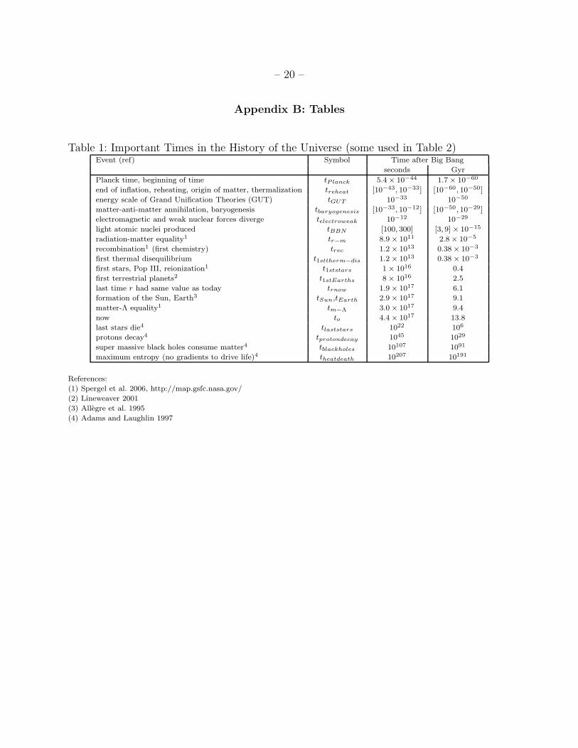
Table 1: Important Times in the History of the Universe (some used in Table 2)Event (ref) Symbol Time after Big Bang

seconds Gyr

Planck time, beginning of time tPlanck 5.4 × 10−44 1.7 × 10−60

end of inflation, reheating, origin of matter, thermalization treheat [10−43, 10−33] [10−60, 10−50]

energy scale of Grand Unification Theories (GUT) tGUT 10−33 10−50

matter-anti-matter annihilation, baryogenesis tbaryogenesis [10−33, 10−12] [10−50, 10−29]

electromagnetic and weak nuclear forces diverge telectroweak 10−12 10−29

light atomic nuclei produced tBBN [100, 300] [3, 9] × 10−15

radiation-matter equality1 tr−m 8.9 × 1011 2.8 × 10−5

recombination1 (first chemistry) trec 1.2 × 1013 0.38 × 10−3

first thermal disequilibrium t1sttherm−dis 1.2 × 1013 0.38 × 10−3

first stars, Pop III, reionization1 t1ststars 1 × 1016 0.4

first terrestrial planets2 t1stEarths 8 × 1016 2.5

last time r had same value as today trnow 1.9 × 1017 6.1

formation of the Sun, Earth3 tSun,tEarth 2.9 × 1017 9.1

matter-Λ equality1 tm−Λ 3.0 × 1017 9.4

now to 4.4 × 1017 13.8

last stars die4 tlaststars 1022 106

protons decay4 tprotondecay 1045 1029

super massive black holes consume matter4 tblackholes 10107 1091

maximum entropy (no gradients to drive life)4 theatdeath 10207 10191

References:

(1) Spergel et al. 2006, http://map.gsfc.nasa.gov/

(2) Lineweaver 2001

(3) Allegre et al. 1995

(4) Adams and Laughlin 1997

– 21 –

Table 2. The probability P (r > ro) of observing r > ro

assuming a uniform distribution of observers Pobs in linear

time, log(time), scale factor and log(scale factor) within the

range ∆x listed.

Range ∆x a P (r > ro) [%]

xmin xmax t log(t) a log(a)

trec 100 Gyr b 8 c 7 0.2 6

tP lanck tlaststars 8 × 10−4 0.6 d 10−104

10−3

tP lanck to 60 c 0.6 50 1

tP lanck t−1P lanck 30 0.3 30 0.5 d

tP lanck theatdeath 10−188 0.1 10−10189

10−188

trec tprotondecay 10−26 1 10−1027

10−26

trec tblackholes 10−88 0.4 10−1089

10−88

trec theatdeath 10−188 0.2 10−10189

10−188

t1ststars tlaststars 8 × 10−4 6 10−104

10−3

t1ststars tprotondecay 10−26 1 10−1027

10−26

t1ststars tblackholes 10−88 0.4 10−1089

10−88

t1ststars theatdeath 10−188 0.2 10−10189

10−188

a See Table 1 for the times corresponding to columns 1 and 2.b The four values in the top row correspond to Fig. 8.

c The two values shown in bold in the t column correspond to the two panels of Fig. 3.d These values correspond to the two panels of Fig.2.

– 22 –

REFERENCES

Adams, F. C. and Laughlin, G. (1997), ‘A dying universe: the long-term fate and evolutionof

astrophysical objects’, Reviews of Modern Physics 69, 337–372.

Aguirre, A., Gratton, S. and Johnson, M. C. (2006), ‘Hurdles for Recent Measures in Eternal

Inflation’, ArXiv hep-th/0611221 .

Aguirre, A. and Tegmark, M. (2005), ‘Multiple universes, cosmic coincidences, and other

dark matters’, Journal of Cosmology and Astro-Particle Physics 1, 3–19.

Allegre, C. J., Manhes, G. and Gopel, C. (1995), ‘The age of the Earth’, Geochim. Cos-

mochim. Acta 59, 1445–1456.

Armendariz-Picon, C., Mukhanov, V. and Steinhardt, P. J. (2000), ‘Dynamical Solution to

the Problem of a Small Cosmological Constant and Late-Time Cosmic Acceleration’,

Physical Review Letters 85, 4438–4441.

Bludman, S. (2004), ‘Tracking quintessence would require two cosmic coincidences’,

Phys. Rev. D 69(12), 122002.

Bludman, S. A. and Roos, M. (2001), ‘Smooth Energy: Cosmological Constant or

Quintessence?’, ApJ 547, 77–81.

Bostrom, N. (2002), Anthropic Bias: Observation Selection Effects in Science and Philoso-

phy, Routledge, London.

Caldwell, R. R., Dave, R. and Steinhardt, P. J. (1998), ‘Cosmological Imprint of an Energy

Component with General Equation of State’, Physical Review Letters 80, 1582–1585.

Carroll, S. M. (2001a), ‘Dark Energy and the Preposterous Universe’, SNAP (SuperNova

Acceleration Probe) Yellow Book astro-ph/0107571 .

Carroll, S. M. (2001b), ‘The Cosmological Constant’, Living Reviews in Relativity 4, 1.

Carter, B. (1983), ‘The anthropic principle and its implications for biological evolution’,

Philosophical Transactions of the Royal Society A 310, 347–363.

Chyba, C. F. (1999), ‘Free Energy for Life on Europa’, AAS/Division for Planetary Sciences

Meeting Abstracts 31, 66.09.

Dicke, R. H. (1961), ‘Dirac’s Cosmology and Mach’s Principle’, Nature 192, 440.

Dirac, P. A. M. (1937), ‘The cosmological constants’, Nature 139, 323.

– 23 –

Dirac, P. A. M. (1938), ‘A New Basis for Cosmology’, Royal Society of London Proceedings

Series A 165, 199–208.

Dodelson, S., Kaplinghat, M. and Stewart, E. (2000), ‘Solving the Coincidence Problem:

Tracking Oscillating Energy’, Physical Review Letters 85, 5276–5279.

Garriga, J., Livio, M. and Vilenkin, A. (2000), ‘Cosmological constant and the time of its

dominance’, Phys. Rev. D 61(2), 023503.

Garriga, J. and Vilenkin, A. (2001), ‘Solutions to the cosmological constant problems’,

Phys. Rev. D 64(2), 023517.

Gunn, J. E. and Gott, J. R. I. (1972), ‘On the Infall of Matter Into Clusters of Galaxies and

Some Effects on Their Evolution’, ApJ 176, 1.

Guo, Z.-K. and Zhang, Y.-Z. (2005), ‘Interacting phantom energy’, Phys. Rev. D

71(2), 023501.

Hopkins, A. M. and Beacom, J. F. (2006), ‘On the Normalization of the Cosmic Star For-

mation History’, ApJ 651, 142–154.

Ida, S. and Lin, D. N. C. (2005), ‘Toward a Deterministic Model of Planetary Formation.

III. Mass Distribution of Short-Period Planets around Stars of Various Masses’, ApJ

626, 1045–1060.

Jaynes, E. T. (1968), ‘Prior Probabilities (p16)’, IEEE Transactions on System Science and

Cybernetics SSC-4, 227–241.

Jordan, P. (1955), Schwerkraft und Weltall, Braunschweig, Braunschweig, Germany.

Lanzetta, K. M., Yahata, N., Pascarelle, S., Chen, H.-W. and Fernandez-Soto, A. (2002),

‘The Star Formation Rate Intensity Distribution Function: Implications for the Cos-

mic Star Formation Rate History of the Universe’, ApJ 570, 492–501.

Linder, E. (1997), First Principles of Cosmology, First Principles of Cosmology, by E.V.

Linder. Addison-Wesley, Harlow, England, 1997.

Lineweaver, C. H. (2001), ‘An Estimate of the Age Distribution of Terrestrial Planets in the

Universe: Quantifying Metallicity as a Selection Effect’, Icarus 151, 307–313.

Lineweaver, C. H. and Davis, T. M. (2002), ‘Does the Rapid Appearance of Life on Earth

Suggest that Life Is Common in the Universe?’, Astrobiology 2, 293–304.

– 24 –

Lineweaver, C. H. and Davis, T. M. (2003), ‘On the Nonobservability of Recent Biogenesis’,

Astrobiology 3, 241–243.

Lineweaver, C. H. and Grether, D. (2003), ‘What Fraction of Sun-like Stars Have Planets?’,

ApJ 598, 1350–1360.

Martel, H., Shapiro, P. R. and Weinberg, S. (1998), ‘Likely Values of the Cosmological

Constant’, ApJ 492, 29.

Nagamine, K., Ostriker, J. P., Fukugita, M. and Cen, R. (2006), ‘The History of Cosmolog-

ical Star Formation: Three Independent Approaches and a Critical Test Using the

Extragalactic Background Light’, ApJ 653, 881–893.

Peacock, J. A. (1999), Cosmological Physics, Cosmological Physics, by John A. Peacock,

pp. 704. ISBN 052141072X. Cambridge, UK: Cambridge University Press, January

1999.

Peebles, P. J. E. (1999), ‘Cosmology: Evolution of the cosmological constant’, Nature

398, 25.

Pogosian, L. and Vilenkin, A. (2007), ‘Anthropic predictions for vacuum energy and neutrino

masses in the light of WMAP-3’, Journal of Cosmology and Astro-Particle Physics

1, 25–+.

Press, W. H. and Schechter, P. (1974), ‘Formation of Galaxies and Clusters of Galaxies by

Self-Similar Gravitational Condensation’, ApJ 187, 425–438.

Seljak, U., Slosar, A. and McDonald, P. (2006), ‘Cosmological parameters from combining

the Lyman-alpha forest with CMB, galaxy clustering and SN constraints’, ArXiv

Astrophysics e-prints .

Spergel, D. N., Bean, R., Dore’, O., Nolta, M. R., Bennett, C. L., Hinshaw, G., Jarosik,

N., Komatsu, E., Page, L., Peiris, H. V., Verde, L., Barnes, C., Halpern, M.,

Hill, R. S., Kogut, A., Limon, M., Meyer, S. S., Odegard, N., Tucker, G. S., Wei-

land, J. L., Wollack, E. and Wright, E. L. (2006), ‘Wilkinson Microwave Anisotropy

Probe (WMAP) Three Year Results: Implications for Cosmology’, astro-ph/0603449

http://lambda.gsfc.nasa.gov/product/map/dr2/params/lcdm-all.cfm .

Steinhardt, P. J. (2003), ‘A quintessential introduction to dark energy’, Royal Society of

London Philosophical Transactions Series A 361, 2497–2513.

Steinhardt, P. J., Wang, L. and Zlatev, I. (1999), ‘Cosmological tracking solutions’,

Phys. Rev. D 59(12), 123504.

– 25 –

Thompson, R. I., Eisenstein, D., Fan, X., Dickinson, M., Illingworth, G. and Kennicutt, Jr.,

R. C. (2006), ‘Star Formation History of the Hubble Ultra Deep Field: Comparison

with the Hubble Deep Field-North’, ApJ 647, 787–798.

Turner, M. S. (2001), ‘Dark Energy’, Nuclear Physics B Proceedings Supplements 91, 405–

409.

Vilenkin, A. (1995a), ‘Making predictions in an eternally inflating universe’, Phys. Rev. D

52, 3365–3374.

Vilenkin, A. (1995b), ‘Predictions from Quantum Cosmology’, Physical Review Letters

74, 846–849.

Vilenkin, A. (1996a), Predictions from Quantum Cosmology, in N. Sanchez and A. Zichichi,

eds, ‘String gravity and physics at the Planck energy scale. Proceedings of the NATO

Advanced Study Institute, Erice, Italy, 8-19 September 1995. Edited by Norma

Sanchez and Antonio Zichichi. Dordrecht: Kluwer Academic Publishers, NATO Ad-

vanced Study Institutes Series. Volume C476’, p. 345.

Vilenkin, A. (1996b), Quantum Cosmology and the Constants of Nature, in K. Sato, T. Sug-

inohara and N. Sugiyama, eds, ‘Cosmological Constant and the Evolution of the

Universe’, p. 161.

Wang, L., Caldwell, R. R., Ostriker, J. P. and Steinhardt, P. J. (2000), ‘Cosmic Concordance

and Quintessence’, ApJ 530, 17–35.

Weinberg, S. (1987), ‘Anthropic bound on the cosmological constant’, Physical Review Let-

ters 59, 2607–2610.

Weinberg, S. (2000), ‘A priori probability distribution of the cosmological constant’,

Phys. Rev. D 61(10), 103505.

Wetherill, G. W. (1996), The Formation Of Habitable Planetary Systems, in L. R. Doyle,

ed., ‘Circumstellar Habitable Zones’, p. 193.

Zlatev, I., Wang, L. and Steinhardt, P. J. (1999), ‘Quintessence, Cosmic Coincidence, and

the Cosmological Constant’, Physical Review Letters 82, 896–899.

This preprint was prepared with the AAS LATEX macros v5.2.