Automated Terrestrial EMI Emitter Detection, Classification ...

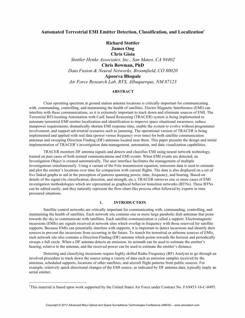
Automated Terrestrial EMI Emitter Detection, Classification, and Localization1

Richard Stottler James Ong Chris Gioia

Stottler Henke Associates, Inc., San Mateo, CA 94402 Chris Bowman, PhD

Data Fusion & Neural Networks, Broomfield, CO 80020 Apoorva Bhopale

Air Force Research Lab, RVS, Albuquerque, NM 87123

ABSTRACT

Clear operating spectrum at ground station antenna locations is critically important for communicating with, commanding, controlling, and maintaining the health of satellites. Electro Magnetic Interference (EMI) can interfere with these communications, so it is extremely important to track down and eliminate sources of EMI. The Terrestrial RFI-locating Automation with CasE based Reasoning (TRACER) system is being implemented to automate terrestrial EMI emitter localization and identification to improve space situational awareness, reduce manpower requirements, dramatically shorten EMI response time, enable the system to evolve without programmer involvement, and support adversarial scenarios such as jamming. The operational version of TRACER is being implemented and applied with real data (power versus frequency over time) for both satellite communication antennas and sweeping Direction Finding (DF) antennas located near them. This paper presents the design and initial implementation of TRACER’s investigation data management, automation, and data visualization capabilities.

TRACER monitors DF antenna signals and detects and classifies EMI using neural network technology, trained on past cases of both normal communications and EMI events. When EMI events are detected, an Investigation Object is created automatically. The user interface facilitates the management of multiple investigations simultaneously. Using a variant of the Friis transmission equation, emissions data is used to estimate and plot the emitter’s locations over time for comparison with current flights. The data is also displayed on a set of five linked graphs to aid in the perception of patterns spanning power, time, frequency, and bearing. Based on details of the signal (its classification, direction, and strength, etc.), TRACER retrieves one or more cases of EMI investigation methodologies which are represented as graphical behavior transition networks (BTNs). These BTNs can be edited easily, and they naturally represent the flow-chart-like process often followed by experts in time pressured situations.

1. INTRODUCTION

Satellite control networks are critically important for communicating with, commanding, controlling, and maintaining the health of satellites. Each network site contains one or more large parabolic dish antennas that point towards the sky to communicate with satellites. Each satellite communication is called a support. Electromagnetic incursions (EMIs) are signals received at network sites which overlap in frequency with those reserved for satellite supports. Because EMIs can potentially interfere with supports, it is important to detect incursions and identify their sources to prevent the incursions from occurring in the future. To search for terrestrial or airborne sources of EMIs, each network site also contains a Direction-Finding (DF) antenna which points towards the horizon and periodically sweeps a full circle. When a DF antenna detects an emission, its azimuth can be used to estimate the emitter’s bearing, relative to the antenna, and the received power can be used to estimate the emitter’s distance.

Detecting and classifying incursions require highly skilled Radio Frequency (RF) Analysts to go through an involved procedure to track down the source using a variety of data such as emission samples received by the antennas, scheduled supports, locations of other satellites, and aircraft flight patterns from public sources. For example, relatively quick directional changes of the EMI source, as indicated by DF antenna data, typically imply an aerial emitter.

1This material is based upon work supported by the United States Air Force under Contract No. FA9453-16-C-0495.

Copyright © 2017 Advanced Maui Optical and Space Surveillance Technologies Conference (AMOS) – www.amostech.com

During normal operations, investigating EMI is labor-intensive. During a conflict, it is especially important to reduce both the labor and elapsed time needed to investigate EMIs. TRACER provides EMI investigation management, automation, and data visualization capabilities to reduce the time and effort needed to detect and classify EMIs.

2. INVESTIGATION DATA MANAGEMENT

For each suspected incursion, TRACER creates an investigation data object which stores the relevant emissions data, other data which supports classification of the incursion, the results of data analyses, and the status and history of the investigation. For example, during real-time monitoring of emissions data, TRACER creates each investigation object when an incursion is first suspected. As TRACER collects and analyzes data, it adds the acquired data and analysis results to the investigation object, providing analysts with rapid access to the data and results related to the investigation of each incursion. Investigation objects can also be used to store data and analyses of historical incursions to enable rapid comparison of new events with incursions which were seen and resolved in the past. Each investigation object contains sub-objects which store emission samples, evidence from various sources, analysis results, actions performed by analysts, and the results of those actions.

Investigation data is stored persistently in a SQL database. Analysts can select a subset of the stored investigations to load into memory for review and updating. The Investigation Viewer, a redacted version of which is shown in Figure 1, is a user interface component which enables the analyst to review and update investigations loaded into memory. The table at the top of this display summarizes the investigation objects that have been loaded into memory, and the lower panes display the details of the investigation selected by the analyst, highlighted in blue.

3. AUTOMATED EMI DETECTION AND CLASSIFICATION

TRACER interfaces with a neural network system called ABNET which analyzes emission samples to detect and classify possible incursions. ABNET is composed of two neural networks. The abnormality detection neural network is trained with examples of normal emission samples in which no incursion is present. This neural network identifies abnormal emission samples which deviate significantly from the normal samples seen during

Figure 1. The TRACER Investigation Viewer displays investigation objects loaded into memory


training. The second neural network is trained with emission samples which have been labelled (classified) by a human expert to indicate various types of emitters. This second network associates a new sample with an emitter type if the sample is similar to training samples previously labelled with that type.

During real-time operations, TRACER retrieves emission samples from each DF antenna and forwards batches of samples to ABNet for analysis. Each abnormal emission sample is added to an existing investigation object, if an appropriate one already exists. If none yet exists, a new investigation is created and initialized with the abnormal sample. Normal samples are also added to existing investigation objects if the investigation contains a recent abnormal sample. These normal samples provide contextual data that can assist the analysis of the abnormal samples.

Currently, TRACER uses the ABNet neural network system developed earlier for the TRACER prototype, as reported in [2]. That version of ABNet detected abnormal emission samples with 97% accuracy and classified samples with 90% accuracy. We plan to develop an improved version of ABNet that uses updated algorithms and training data sets.

4. INVESTIGATION AUTOMATION AND WORKFLOW MANAGEMENT

TRACER automates some of the gathering and analysis of data. For example, TRACER automatically queries flight databases to retrieve the paths of flights in the estimated vicinity of the suspected emitter.

TRACER also creates investigation sub-objects which specify actions that the human analyst must perform to gather or analyze data. Analysts use the Human Action Viewer to read and follow the instructions specified by each action, such as asking for information from an organization or querying an online database. Analysts enter text or select from menus to save the results of each action which are then stored in the investigation object.

The Investigator is implemented using the open source SimBionic intelligent agent toolkit. SimBionic enables users to define control logic as one or more Behavior Transition Networks (BTNs) running in parallel. Each BTN is like a flow chart or finite state machine, augmented with features which enhance its power. These features include the ability to set/get local and global variables and call JavaScript functions and Java methods. These BTNs call Java methods provided by other TRACER components to: • Query and update investigation objects and sub-objects, • Query external data sources and check their results, • Carry out analyses, and • Add actions to the queue of human actions and continue investigation based on their results.

TRACER’s use of SimBionic to automate investigation tasks and manage workflow is further described in [2].

5. DATA VISUALIZATION

TRACER provides two data visualization components. The Emission Data Display is an integrated collection of graphical data displays which helps analysts see multivariate patterns in emission sample data. The Map Display shows emitter locations estimated from DF antenna emission samples and other geolocated data.

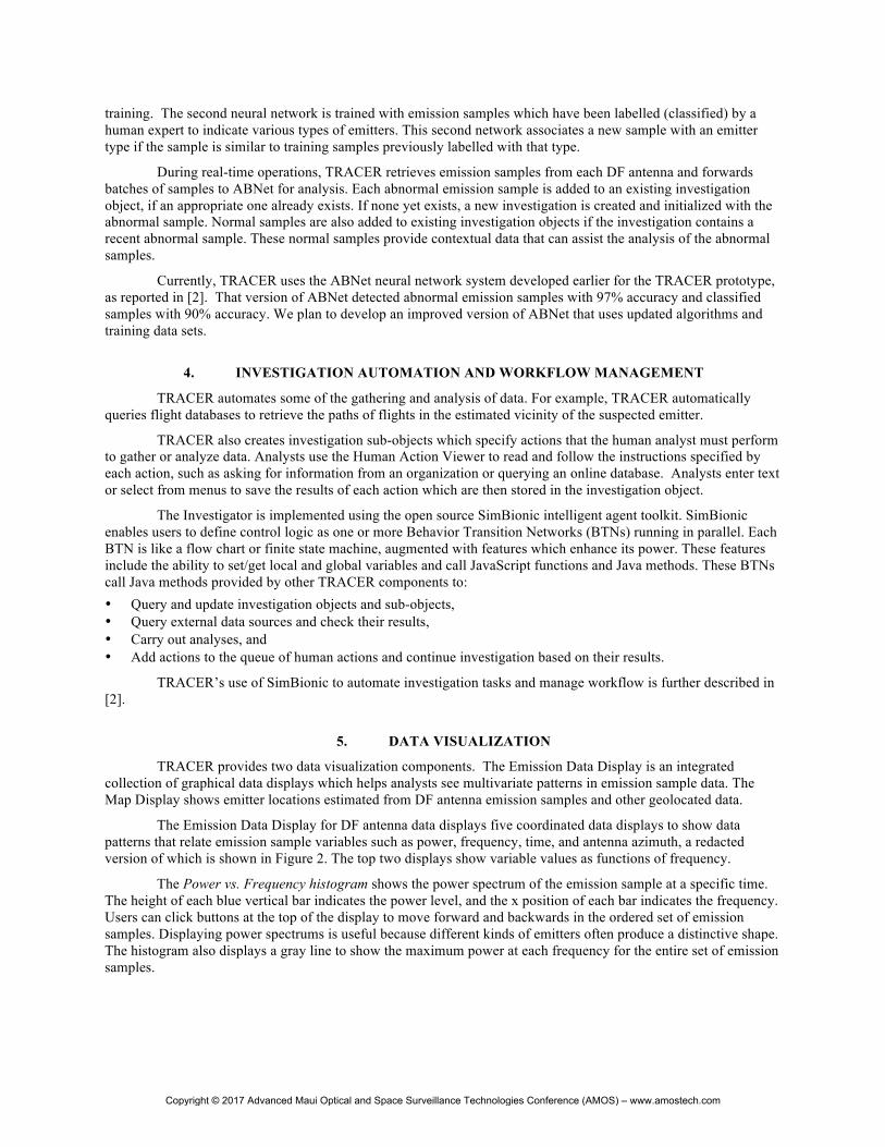
The Emission Data Display for DF antenna data displays five coordinated data displays to show data patterns that relate emission sample variables such as power, frequency, time, and antenna azimuth, a redacted version of which is shown in Figure 2. The top two displays show variable values as functions of frequency.

The Power vs. Frequency histogram shows the power spectrum of the emission sample at a specific time. The height of each blue vertical bar indicates the power level, and the x position of each bar indicates the frequency. Users can click buttons at the top of the display to move forward and backwards in the ordered set of emission samples. Displaying power spectrums is useful because different kinds of emitters often produce a distinctive shape. The histogram also displays a gray line to show the maximum power at each frequency for the entire set of emission samples.


In the Power vs. Azimuth and Frequency scatterplot, each blue circle represents an emission sample. The x position of each circle indicates the frequency at which power is highest, and the y position indicates the DF antenna azimuth. Brighter circles indicate emission samples with higher power. This graph is useful because data points representing samples from the same emitter often have similar frequencies and azimuths, so clusters of data points often suggest multiple samples from the same emitter.

The bottom three displays show variable values as functions of time. In the Max Power vs. Time bar graph, each vertical bar represents an emission sample. The height of each bar shows the maximum signal level across all frequencies in each sample, and the x position indicates the sample’s time. This graph is useful for summarizing how emission sample power levels vary over time.

Figure 2. The Emission Data Display uses linked displays to show complex patterns in emission sample data.


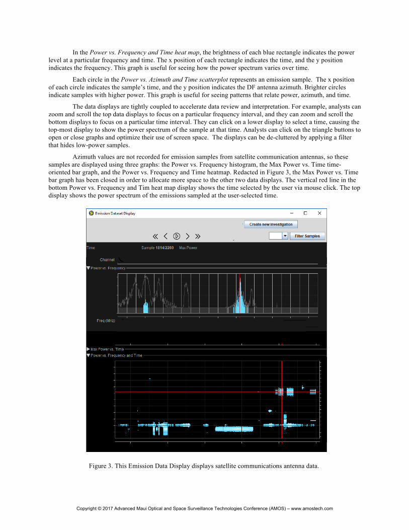
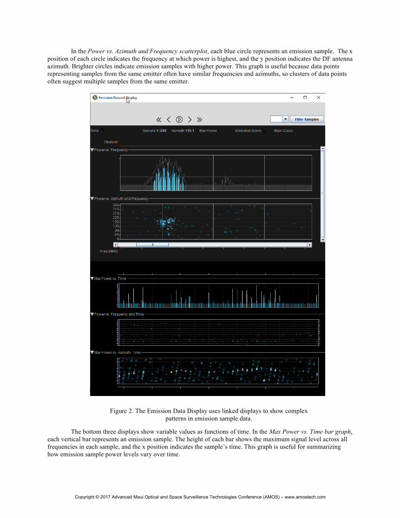
In the Power vs. Frequency and Time heat map, the brightness of each blue rectangle indicates the power level at a particular frequency and time. The x position of each rectangle indicates the time, and the y position indicates the frequency. This graph is useful for seeing how the power spectrum varies over time.

Each circle in the Power vs. Azimuth and Time scatterplot represents an emission sample. The x position of each circle indicates the sample’s time, and the y position indicates the DF antenna azimuth. Brighter circles indicate samples with higher power. This graph is useful for seeing patterns that relate power, azimuth, and time.

The data displays are tightly coupled to accelerate data review and interpretation. For example, analysts can zoom and scroll the top data displays to focus on a particular frequency interval, and they can zoom and scroll the bottom displays to focus on a particular time interval. They can click on a lower display to select a time, causing the top-most display to show the power spectrum of the sample at that time. Analysts can click on the triangle buttons to open or close graphs and optimize their use of screen space. The displays can be de-cluttered by applying a filter that hides low-power samples.

Azimuth values are not recorded for emission samples from satellite communication antennas, so these samples are displayed using three graphs: the Power vs. Frequency histogram, the Max Power vs. Time time-oriented bar graph, and the Power vs. Frequency and Time heatmap. Redacted in Figure 3, the Max Power vs. Time bar graph has been closed in order to allocate more space to the other two data displays. The vertical red line in the bottom Power vs. Frequency and Tim heat map display shows the time selected by the user via mouse click. The top display shows the power spectrum of the emissions sampled at the user-selected time.

Figure 3. This Emission Data Display displays satellite communications antenna data.


It can be difficult to see significant patterns that relate many variables such as time, power, frequency, and DF antenna azimuth. To help analysts see patterns in high-dimensional data, we added a brushing capability that enables users to see patterns spanning multiple linked graphs in the Emission Data Display. For example, users can click and drag the mouse in the Azimuth vs. Frequency scatterplot to select a rectangular area containing samples within an azimuth range and maximum power frequency range, as shown, redacted, in Figure 4. The bottom Azimuth vs. Time graph then highlights data points that represent the selected emission samples by drawing green circles around them. The brushing is bi-directional: users can also select a rectangle of data points in the Azimuth vs. Time graph to highlight the data points in the Azimuth vs. Frequency scatterplot that represent the same emission samples.

Figure 4. The Emission Data Display uses brushing to highlight user-selected samples in multiple displays.


TRACER uses a clustering algorithm to group emission samples that might be detecting the same emitter. The algorithm computes the similarity between each pair of samples, based on their power spectrums, azimuths, and relative timing. To compare power spectrums, TRACER models each spectrum as a vector, one dimension per frequency, and computes their normalized dot product similarity. Analysts can select menu items to highlight the emission samples in each cluster. Figure 5 shows a redacted example in which some emission samples have been grouped into the same cluster and are highlighted in violet in two scatterplots.

TRACER uses a variant of the Friis equation to estimate the distance between the emitter and the DF

antenna at the time of each sample. The bearing of the emitter, relative to the DF antenna, is assumed to equal the antenna’s azimuth when the emission was sampled. If consecutive samples have similar power spectrums, we assume that the samples are detecting the same emitter so that the emitter bearing equals the azimuth of the sample with the highest power. This rule assumes that the received emissions are strongest when the DF antenna points

Figure 5. The Emission Data Display highlights in violet the emission samples in the same cluster which are likely to be emitted by the same source.


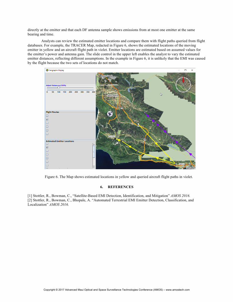
directly at the emitter and that each DF antenna sample shows emissions from at most one emitter at the same bearing and time.

Analysts can review the estimated emitter locations and compare them with flight paths queried from flight databases. For example, the TRACER Map, redacted in Figure 6, shows the estimated locations of the moving emitter in yellow and an aircraft flight path in violet. Emitter locations are estimated based on assumed values for the emitter’s power and antenna gain. The slide control in the upper left enables the analyst to vary the estimated emitter distances, reflecting different assumptions. In the example in Figure 6, it is unlikely that the EMI was caused by the flight because the two sets of locations do not match.

6. REFERENCES [1] Stottler, R., Bowman, C., “Satellite-Based EMI Detection, Identification, and Mitigation” AMOS 2016. [2] Stottler, R., Bowman, C., Bhopale, A. “Automated Terrestrial EMI Emitter Detection, Classification, and Localization” AMOS 2016.

Figure 6. The Map shows estimated locations in yellow and queried aircraft flight paths in violet.


Automated Terrestrial EMI Emitter Detection, Classification ...

Documents

Transcript of Automated Terrestrial EMI Emitter Detection, Classification ...