A&A 508, 1509–1516 (2009)DOI: 10.1051/0004-6361/200912378c© ESO 2009

Astronomy&

Astrophysics

Transit detections of extrasolar planets aroundmain-sequence stars

I. Sky maps for hot Jupiters�

R. Heller1, D. Mislis1, and J. Antoniadis2

1 Hamburger Sternwarte (Universität Hamburg), Gojenbergsweg 112, 21029 Hamburg, Germanye-mail: [rheller;dmislis]@hs.uni-hamburg.de

2 Aristotle University of Thessaloniki, Dept. of Physics, Section of Astrophysics, Astronomy and Mechanics,541 24 Thessaloniki, Greecee-mail: iantonia@physics.auth.gr

Received 23 April 2009 / Accepted 3 October 2009

ABSTRACT

Context. The findings of more than 350 extrasolar planets, most of them nontransiting Hot Jupiters, have revealed correlations betweenthe metallicity of the main-sequence (MS) host stars and planetary incidence. This connection can be used to calculate the planetformation probability around other stars, not yet known to have planetary companions. Numerous wide-field surveys have recentlybeen initiated, aiming at the transit detection of extrasolar planets in front of their host stars. Depending on instrumental propertiesand the planetary distribution probability, the promising transit locations on the celestial plane will differ among these surveys.Aims. We want to locate the promising spots for transit surveys on the celestial plane and strive for absolute values of the expectednumber of transits in general. Our study will also clarify the impact of instrumental properties such as pixel size, field of view (FOV),and magnitude range on the detection probability.Methods. We used data of the Tycho catalog for ≈1 million objects to locate all the stars with 0m � mV � 11.5m on the celestial plane.We took several empirical relations between the parameters listed in the Tycho catalog, such as distance to Earth, mV, and (B−V), andthose parameters needed to account for the probability of a star to host an observable, transiting exoplanet. The empirical relationsbetween stellar metallicity and planet occurrence combined with geometrical considerations were used to yield transit probabilitiesfor the MS stars in the Tycho catalog. Magnitude variations in the FOV were simulated to test whether this fluctuations would bedetected by BEST, XO, SuperWASP and HATNet.Results. We present a sky map of the expected number of Hot Jupiter transit events on the basis of the Tycho catalog. Conditioned bythe accumulation of stars towards the galactic plane, the zone of the highest number of transits follows the same trace, interrupted byspots of very low and high expectation values. The comparison between the considered transit surveys yields significantly differingmaps of the expected transit detections. While BEST provides an unpromising map, those for XO, SuperWASP, and HATNet showFsOV with up to 10 and more expected detections. The sky-integrated magnitude distribution predicts 20 Hot Jupiter transits withorbital periods between 1.5 d and 50 d and mV < 8m, of which two are currently known. In total, we expect 3412 Hot Jupiter transitsto occur in front of MS stars within the given magnitude range. The most promising observing site on Earth is at latitude = −1.

Key words. planetary systems – occultations – solar neighborhood – Galaxy: abundances – instrumentation: miscellaneous –methods: observational

1. Introduction

A short essay by Otto Struve (Struve 1952) provided the firstpublished proposal of transit events as a means of exoplane-tary detection and exploration. Calculations for transit detec-tion probabilities (Rosenblatt 1971; Borucki & Summers 1984;Pepper & Gaudi 2006) and for the expected properties of thediscovered planets have been done subsequently by many others(Gillon et al. 2005; Fressin et al. 2007; Beatty & Gaudi 2008).Until the end of the 1990s, when the sample of known exoplan-ets had grown to more than two dozen (Castellano et al. 2000),the family of so-called “Hot Jupiters”, with 51 Pegasi as theirprototype, was unknown and previous considerations had been

� Sky maps (Figs. 1 and 3) can be downloaded in electronic form atthe CDS via anonymous ftp tocdsarc.u-strasbg.fr (130.79.128.5) or viahttp://cdsweb.u-strasbg.fr/cgi-bin/qcat?J/A+A/508/1509

based on systems similar to the solar system. Using geometricalconsiderations, Rosenblatt (1971)1 found that the main contri-bution to the transit probability of a solar system planet wouldcome from the inner rocky planets. However, the transits of theserelatively tiny objects remain undetectable around other stars asyet.

The first transit of an exoplanet was finally detectedaround the sun-like star HD209458 (Charbonneau et al. 2000;Queloz et al. 2000). Thanks to the increasing number of ex-oplanet search programs, such as the ground-based OpticalGravitational Lensing Experiment (OGLE) (Udalski et al. 1992),the Hungarian Automated Telescope (HAT) (Bakos et al. 2002,2004), the Super Wide Angle Search for Planets (SuperWASP)(Street et al. 2003), the Berlin Exoplanet Search Telescope(BEST) (Rauer et al. 2004), XO (McCullough et al. 2005), the

1 A correction to his Eq. (2) is given in Borucki & Summers (1984).

Article published by EDP Sciences

1510 R. Heller et al.: Transit detections of extra-solar planets. I.

Transatlantic Exoplanet Survey (TrES) (Alonso et al. 2007), andthe Tautenburg Exoplanet Search Telescope (TEST) (Eigmüller& Eislöffel 2009) and the space-based missions “Convection,Rotation & Planetary Transits” (CoRoT) (Baglin et al. 2002)and Kepler (Christensen-Dalsgaard et al. 2007), the number ofexoplanet transits has grown to 62 until September 1st 20092

and will grow drastically within the next years. These transit-ing planets have very short periods, typically <10 d, and verysmall semimajor axes of usually <0.1 AU, which is a selectioneffect based on geometry and Kepler’s third law (Kepler et al.1619). Transiting planets with longer periods present more ofa challenge, since their occultations are less likely in terms ofgeometrical considerations and they occur less frequently.

Usually, authors of studies on the expected yield of tran-sit surveys generate a fictive stellar distribution based on stel-lar population models. Fressin et al. (2007) use a Monte-Carloprocedure to synthesize a fictive stellar field for OGLE basedon star counts from Gould et al. (2006), a stellar metallicity dis-tribution from Nordström et al. (2004), and a synthetic struc-ture and evolution model of Robin et al. (2003). The metallicitycorrelation, however, turned out to underestimate the true stellarmetallicity by about 0.1 dex, as found by Santos et al. (2004)and Fischer & Valenti (2005). In their latest study, Fressin et al.(2009) first generate a stellar population based on the Besançoncatalog from Robin et al. (2003) and statistics for multiple sys-tems from Duquennoy & Mayor (1991) to apply then the metal-licity distribution from Santos et al. (2004) and issues of de-tectability (Pont et al. 2006). Beatty & Gaudi (2008) rely on aGalactic structure model by Bahcall & Soneira (1980), a massfunction as suggested by Reid et al. (2002) based on Hipparcosdata, and a model for interstellar extinction to estimate the over-all output of the current transit surveys TrES, XO, and Kepler.In their paper on the number of expected planetary transits to bedetected by the upcoming Pan-STARRS survey (Kaiser 2004),Koppenhoefer et al. (2009) also used a Besançon model as pre-sented in Robin et al. (2003) to derive a brightness distribution ofstars in the target field and performed Monte-Carlo simulationsto simulate the occurrence and detections of transits. These stud-ies include detailed observational constraints such as observingschedule, weather conditions, and exposure time and issues ofdata reduction, e.g. red noise and the impact of the instrument’spoint spread function.

In our study, we rely on the extensive data reservoir of theTycho catalog instead of assuming a stellar distribution or aGalactic model. We first estimate the number of expected ex-oplanet transit events as a projection on the complete celestialplane. We refer to recent results of transit surveys such as sta-tistical, empirical relationships between stellar properties andplanetary formation rates. We then use basic characteristics ofcurrent low-budget but high-efficiency transit programs (BEST,XO, SuperWASP, and HATNet), regardless of observational con-straints mentioned above, and a simple model to test putativetransits with the given instruments. With this procedure, we yieldsky maps, which display the number of expected exoplanet tran-sit detections for the given surveys, i.e. the transit sky as it isseen through the eyeglasses of the surveys.

The Tycho catalog comprises observations of roughly 1 mil-lion stars taken with the Hipparcos satellite between 1989 and1993 (ESA 1997; Hoeg 1997). During the survey, roughly100 observations were taken per object. From the derivedastrometric and photometric parameters, we use the right

2 Extrasolar Planets Encyclopedia (EPE): www.exoplanet.eu. Fourof these 62 announced transiting planets have no published position.

ascension (α), declination (δ), the color index (B − V), the ap-parent visible magnitude mV, and the stellar distance d that havebeen calculated from the measured parallax. The catalog is al-most complete for the magnitude limit mV � 11.5m, but wealso find some fainter stars in the list.

2. Data analysis

The basis of our analysis is a segmentation of the celestial planeinto a mosaic made up of multiple virtual fields of view (FsOV).In a first approach, we subdivide the celestial plane into a setof 181 × 361 = 65 341 fields. Most of the current surveys donot use telescopes, which typically have small FsOV, but lenseswith FsOV of typically 8◦ × 8◦. Thus, we apply this extension of8◦ × 8◦ and a stepsize of Δδ = 1◦ = Δα, with an overlap of 7◦between adjacent fields, for our automatic scanning in order tocover the complete sky. We chose the smallest possible step sizein order to yield the highest possible resolution and the finestscreening, despite the high redundancy due to the large overlap.A smaller step size than 1◦ was not convenient due to limitationsof computational time. An Aitoff projection is used to fold thecelestial sphere onto a 2D sheet.

2.1. Derivation of the stellar parameters

One key parameter for all of the further steps is the effectivetemperature Teff of the stars in our sample. This parameter is notgiven in the Tycho catalog but we may use the stellar color index(B − V) to deduce Teff by

Teff = 10[14.551−(B−V)]/3.684 K, (1)

which is valid for main-sequence (MS) stars with Teff � 9100 Kas late as type M8 (Reed 1998). Although we apply this equa-tion to each object in the catalog, of which a significant frac-tion might exceed Teff = 9100 K, this will not yield a seriouschallenge since we will dismiss these spurious candidates below.From the object’s distance to Earth d and the visible magnitudemV, we derive the absolute visible magnitude MV via

MV = mV − 5m log

(d

10 pc

), (2)

where we neglected effects of stellar extinction. In the next step,we compute the stellar radius R� in solar units via

R�R�=

⎡⎢⎢⎢⎢⎢⎣(

5770 KTeff

)4

10(4.83−MV)/2.5

⎤⎥⎥⎥⎥⎥⎦1/2

(3)

and the stellar mass M� by

M� =(4πR2

�σSBT 4eff

)1/β, (4)

where σSB is the Stefan-Boltzmann constant. The coefficient βin the relation L ∝ Mβ depends on the stellar mass. We use thevalues and mass regimes that were empirically found by Cesteret al. (1983), which are listed in Table 1 (see also Smith 1983).

We deduce the stellar metallicity [Fe/H]� from the star’s ef-fective temperature Teff and its color index (B − V) by

[Fe/H]�=1

411

(Teff

K−8423+4736(B− V)−1106 (B−V)2

), (5)

as given in Santos et al. (2004). This relation, however, is onlyvalid for stars with 0.51 < (B − V) < 1.33, 4495 K < Teff <6339 K, −0.7 < [Fe/H]� < 0.43, and log(g) > 4. We reject

R. Heller et al.: Transit detections of extra-solar planets. I. 1511

Table 1. Empirical values for β in the mass-luminosity relation Eq. (4)as given in Cester et al. (1983).

β Stellar mass regime

3.05 ± 0.14 M� � 0.5 M�4.76 ± 0.01 0.6 M� � M� � 1.5 M�3.68 ± 0.05 1.5 M� � M�

those stars from the sample that do not comply with all theseboundary conditions. On the one hand we cleanse our sampleof non-MS stars, on the other hand the sample is reduced seri-ously. While our original reservoir, our “master sample”, con-sists of 1 031 992 stars from the Tycho catalog, all the restric-tions mentioned above diminish our sample to 392 000 objects,corresponding to roughly 38%.

3. Transit occurrence and transit detection

3.1. Transit occurrence

Now that we derived the fundamental stellar parameters, we mayturn towards the statistical aspects of planetary occurrence, ge-ometric transit probability and transit detection. We start withthe probability for a certain star of the Tycho catalog, say theith star, to host an exoplanet. For F, G, and K dwarfs with−0.5 < [Fe/H]i < 0.5, Fischer & Valenti (2005) found the em-pirical relationship

℘∃ planet,i = 0.03 · 102·[Fe/H]i (6)

for a set of 850 stars with an analysis of Doppler measurementssufficient to detect exoplanets with radial velocity (RV) semi-amplitudes K > 30 ms−1 and orbital periods shorter than 4 yr(see Marcy et al. 2005; Wyatt et al. 2007, for a discussion ofthe origin of this formula and its implications for planet forma-tion). These periods are no boundary conditions for our simu-lations since we are only interested in surveys with observingperiods of ≤50 d. The additional constraint on the metallicitydoes not reduce our diminished sample of 392 000 stars sincethere is no star with −0.7 < [Fe/H]i < −0.5 in the Tycho cat-alog. Similar to the correlation we use, Udry & Santos (2007)found a metallicity distribution of exoplanet host stars equiva-lent to ℘∃ planet,i = 0.044 × 102.04·[Fe/H]i . However, this fit was re-stricted to stars with [Fe/H]� > 0 since they suspect two regimesof planet formation. Sozzetti et al. (2009) extended the uniformsample of Fischer & Valenti (2005) and found the power-law℘∃ planet,i = 1.3×102·[Fe/H]i +C, C ∈ {0, 0.5}, to yield the best datafit. These recent studies also suggest that there exists a previ-ously unrecognized tail in the planet-metallicity distribution for[Fe/H]� < 0. Taking Eq. (6) we thus rather underestimate thetrue occurrence of exoplanets around the stars from the Tychocatalog. The metallicity bias of surveys using the RV method forthe detection of exoplanets is supposed to cancel out the bias oftransit surveys (Gould et al. 2006; Beatty & Gaudi 2008).

In the next step, we analyze the probability of the putativeexoplanet to actually show a transit. Considering arbitrary incli-nations of the orbital plane with respect to the observer’s lineof sight and including Kepler’s third law, Gilliland et al. (2000)found the geometric transit probability to be

℘geo,i = 23.8

(Mi

M�

)−1/3 (Ri

R�

) (Pd

)−2/3

, (7)

where P is the orbital period. A more elaborate expression –including eccentricity, planetary radius, the argument of perias-tron and the semi-major axis instead of the orbital period – isgiven by Seagroves et al. (2003). Note that ℘geo,i in Eq. (7) doesnot explicitly but implicitly depend on the semi-major axis a viaP = P(a)! The probability for an exoplanetary transit to occuraround the ith star is then given by

℘occ,i = ℘∃ planet,i · ℘geo,i, (8)

where P is the remaining free parameter, all the other parametersare inferred from the Tycho data. Since we are heading for theexpectation value, i.e. the number of expected transits in a cer-tain field of view (FOV), we need a probability density for thedistribution of the orbital periods of extrasolar planets. On thebasis of the 233 exoplanets listed in the EPE on July 6th 2007,Jiang et al. (2007) used a power-law fit δ(P) = C(k) · (P/d)−k,with C(k) as the normalization function, and the boundary con-dition for the probability density

∫ ∞0

dPδ(P) = 1 to get

δ(P) =1 − k

B1−k − A1−k

(Pd

)−k

(9)

with A = 1.211909 d and B = 4517.4 d as the lower and upperlimits for the period distribution and k = 0.9277. This functionis subject to severe selection effects and bases on data obtainedfrom a variety of surveys and instruments. It overestimates short-period planets since Jiang et al. (2007) included transiting plan-ets and the associated selection effects. While the function pre-sumably does not mirror the true distribution of orbital periodsof exoplanets, it is correlated to the period distribution to whichcurrent instruments are sensitive, in addition to geometric selec-tion effects as given by Eq. (7).

We now segment the celestial plane into a mosaic made up ofmultiple virtual FsOV, as described at the beginning of Sect. 2, tocalculate the number of expected transits in that field. In Sect. 3.2we will attribute the FOV of the respective instrument to that mo-saic and we will also consider the CCD resolution. The numberof stars comprised by a certain FOV is n. The number of ex-pected transits around the ith star in that field, Ni, with periodsbetween P1 and P2 is then given by

Ni =

∫ P2

P1

dP δ(P) ℘occ,i (10)

= ℘∃ planet,i · 23.8

(Mi

M�

)−1/3 (Ri

R�

)1 − k

B1−k − A1−k

× 11/3 − k

(P1/3−k

2 − P1/3−k1

)d2/3 | A<P1<P2<B ,

and the number of expected transits in the whole FOV is

N =n∑

i=1

Ni . (11)

We emphasize that this is not yet the number of expected transitdetections within a certain FOV (see Sect. 4) but the number ofexpected transits to occur within it.

A graphical interpretation of this analysis is presented inFig. 1, where we show a sky map of the expected number ofexoplanet transits around MS stars with mV � 11.5m for orbitalperiods between P1 = 1.5 d and P2 = 50 d. This map bases onseveral empirical relationships and on substantial observationalbias towards close-in Jupiter-like planets, but nevertheless it rep-resents the transit distribution to which current instrumentation

1512 R. Heller et al.: Transit detections of extra-solar planets. I.

Fig. 1. Sky map of the expected number of exoplanet transit events, N,with orbital periods between P1 = 1.5 d and P2 = 50 d on the basis of392 000 objects from the Tycho catalog. The published positions of 58transiting planets from the EPE as of September 1st 2009 are indicatedwith symbols: 6 detections from the space-based CoRoT mission arelabeled with triangles, 52 ground-based detections marked with squares.The axes only refer to the celestial equator and meridian.

has access to. The pronounced bright regions at the upper leftand the lower right are the anti-center and the center of the MilkyWay, respectively. The absolute values of 0.5 � N � 5 for themost of the sky are very well in line with the experiences fromwide-field surveys using a 6◦ × 6◦ field. Mandushev et al. (2005)stated 5 to 20 or more exoplanet transit candidates, dependingon Galactic latitude, and a ratio of ≈25:1 between candidatesand confirmed planets, which is equivalent to 0.2 � N � 1. Ourvalues are a little higher, probably due to the slightly larger FOVof 8◦ × 8◦ used in Fig. 1 and due to the effect of blends andunresolved binaries (see discussion in Sect. 5).

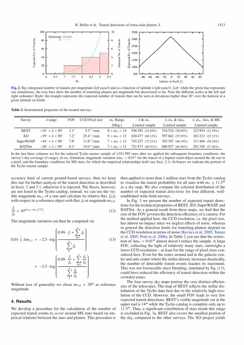
In the left panel of Fig. 2, we show the distribution of ex-pected transits from our simulation as a function of the hoststars’ magnitudes compared to the distribution of the observedtransiting exoplanets. The scales for both distributions differabout an order of magnitude, which is reasonable since only afraction of actual transits is observed as yet. For mV < 8m, onlyHD209458b and HD189733b are currently know to show tran-sits whereas we predict 20 of such transits with periods between1.5 d and 50 d to occur in total. We also find that the numberof detected transiting planets does not follow the shape of thesimulated distribution for mV > 9m. This is certainly induced bya lack of instruments with sufficient sensitivity towards higherapparent magnitudes, the much larger reservoir of fainter starsthat has not yet been subject to continuous monitoring, and thehigher demands on transit detection pipelines.

Our transit map allows us to constrain convenient locationsfor future ground-based surveys. A criterion for such a loca-tion is the number of transit events that can be observed froma given spot at latitude l on Earth. To yield an estimate, we inte-grate N over that part of the celestial plane that is accessablefrom a telescope situated at l. We restrict this observable fanto l − 60◦ < δ < l + 60◦, implying that stars with elevations>30◦ above the horizon are observable. The number of the tran-sit events with mV � 11.5m that is observable at a certain latitudeon Earth is shown in the right panel of Fig. 2. This distribu-tion resembles a triangle with its maximum almost exactly at theequator. Its smoothness is caused by the wide angle of 120◦ thatflattens all the fine structures that can be seen in Fig. 1.

3.2. Transit detection

So far, we have computed the sky and magnitude distributionsof expected exoplanet transits with orbital periods between 1.5 dand 50 d, based on the stellar parameters from the Tycho dataand empirical relations. In order to estimate if a possible tran-sit can actually be observed, one also has to consider technicalissues of a certain telescope as well as the efficiency and the se-lection effects of the data reduction pipelines. The treatment ofthe pipeline will not be subject of our further analysis. The rel-evant aspects for our concern are the pixel size of the CCD, itsFOV, the mV range of the CCD-telescope combination, and thedeclination fan that is covered by the telescope.

To detect a transit, one must be able to distinguish the pe-riodic transit pattern within a light curve from the noise in thedata. Since the depth of the transit curve is proportional tothe ratio AP/A�, where AP and A� are the sky-projected areas ofthe planet and the star, respectively, and RP/R� =

√AP/A�, with

RP as the planetary radius, the detection probability for a cer-tain instrument is also restricted to a certain regime of planetaryradii. Assuming that the transit depth is about 1%, the planetaryradius would have to be larger than ≈R�/10. We do not includean elaborate treatment of signal-to-noise in our considerations(see Aigrain & Pont 2007). Since our focus is on MS stars andour assumptions for planetary occurrence are based on those ofHot Jupiters, our argumentation automatically leads to planetarytransits of exoplanets close to ≈R�/10.

We also do not consider observational aspects, such as inte-gration time and an observer on a rotating Earth with observationwindows and a finite amount of observing time (see Fleminget al. 2008, for a review of these and other observational as-pects). Instead, we focus on the technical characteristics of fourwell-established transit surveys and calculate the celestial distri-bution of expected exoplanet transit detections in principle byusing one of these instruments. The impact of limited observ-ing time is degraded to insignificance because the span of orbitalperiods we consider in Eq. (10) reaches only up to P2 = 50 d.After repeated observations of the same field, such a transitingcompanion would be detected after �3 yr, which is the typicalduty cycle of current surveys.

Our computations are compared for four surveys: BEST,XO, SuperWASP, and HATNet. This sample comprises the threemost fruitful surveys in terms of first planet detections and BEST– a search program that used a telescope instead of lenses.While observations with BEST have been ceased without anyconfirmed transit detection, XO has announced detections andSuperWASP and HATNet belong the most fruitful surveys todate. An overview of the relevant observational and technicalproperties of these surveys is given in Table 2. For each sur-vey, we first restrict the Tycho master sample to the respectivemagnitude range, yielding an mV-restricted sample. In the nextstep, we virtually observe the subsample with the fixed FOV ofthe survey telescope, successively grazing the whole sky withsteps of 1◦ between adjacent fields. The FOV is composed ofa number of CCD pixels and each of these pixels contains acertain number of stars, whose combined photon fluxes mergeinto a count rate. Efficient transit finding has been proven tobe possible from the ground in crowded fields, where target ob-jects are not resolved from neighbor stars. To decide whether ahypothetical transit around the ith star in the pixel would be de-tected, we simulate the effect of a transiting object that reducesthe light flux contribution li of the ith star on the combined flux∑n

k lk of the stars within a pixel. If the ith magnitude variationon the pixel-combined light is ΔmV,i ≥ 0.01m, which is a typical

R. Heller et al.: Transit detections of extra-solar planets. I. 1513

Fig. 2. Sky-integrated number of transits per magnitude (left panel) and as a function of latitude (right panel). Left: while the green line representsour simulations, the rosy bars show the number of transiting planets per magnitude bin discovered so far. Note the different scales at the left andright ordinates! Right: the triangle represents the expected number of transits that can be seen at elevations higher than 30◦ over the horizon at agiven latitude on Earth.

Table 2. Instrumental properties of the treated surveys.

Survey δ range FOV CCD Pixel size mV Range δ & mV δ, mV & ΔmV δ, mV, ΔmV & MS

[Mag.] Limited sample Limited sample Limited sample

BEST −16◦ < δ < 90◦ 3.1◦ 5.5 ′′/mm 8 < mV < 14 546 382 (52.94%) 516 524 (50.05%) 222 854 (21.59%)

XO −39◦ < δ < 90◦ 7.2◦ 25.4 ′′/mm 9 < mV < 12 620 477 (60.12%) 597 842 (57.93%) 263 213 (25.51%)

SuperWASP −44◦ < δ < 90◦ 7.8◦ 13.8 ′′/mm 7 < mV < 12 745 227 (72.21%) 703 707 (68.19%) 311 404 (30.18%)

HATNet −28◦ < δ < 90◦ 8.3◦ 14.0 ′′/mm 7 < mV < 12 721 473 (69.91%) 686 927 (66.56%) 283 350 (27.46%)

In the last three columns we list the reduced Tycho master sample of 1 031 992 stars after we applied the subsequent boundary conditions: thesurvey’s sky-coverage (δ range), its mV limitation, magnitude variation ΔmV > 0.01m for the transit of a Jupiter-sized object around the ith star ina pixel, and the boundary conditions for MS stars, for which the empirical relationships hold (see Sect. 2.1). In braces we indicate the portion ofthe Tycho master sample.

accuracy limit of current ground-based surveys, then we keepthis star for further analysis of the transit detection as describedin Sects. 2 and 3.1, otherwise it is rejected. The fluxes, however,are not listed in the Tycho catalog; instead, we can use the vis-ible magnitude mV,i of a star and calculate its relative flux fi/ f0with respect to a reference object with flux f0 at magnitude mV,0:

fif0= 10(mV,0−mV,i)/2.5. (12)

The magnitude variation can then be computed via

0.01!≤ ΔmV,i = −2.5 · log

⎛⎜⎜⎜⎜⎜⎜⎜⎜⎜⎜⎜⎜⎜⎜⎜⎜⎜⎜⎝

0.99 · fi +n∑

k�i

fk

n∑k

fk

⎞⎟⎟⎟⎟⎟⎟⎟⎟⎟⎟⎟⎟⎟⎟⎟⎟⎟⎟⎠(13)

= −2.5 · log

⎛⎜⎜⎜⎜⎜⎜⎜⎜⎜⎜⎜⎜⎜⎜⎜⎜⎜⎜⎝

0.99 · fif0+

n∑k�i

fkf0

n∑k

fkf0

⎞⎟⎟⎟⎟⎟⎟⎟⎟⎟⎟⎟⎟⎟⎟⎟⎟⎟⎟⎠·

Without loss of generality we chose mV,0 = 30m as referencemagnitude.

4. Results

We develop a procedure for the calculation of the number ofexpected transit events to occur around MS stars based on em-pirical relations between the stars and planets. This procedure is

then applied to more than 1 million stars from the Tycho catalogto visualize the transit probability for all stars with mV � 11.5m

as a sky map. We also compute the celestial distribution of thenumber of expected transit detections for four different, well-established wide-field surveys.

In Fig. 3 we present the number of expected transit detec-tions for the technical properties of BEST, XO, SuperWASP, andHATNet. As a general result from these maps, we find that thesize of the FOV governs the detection efficiency of a camera. Forthe method applied here, the CCD resolution, i.e. the pixel size,has almost no impact since we neglect effects of noise, whereasin general the detection limits for transiting planets depend onthe CCD resolution in terms of noise (Kovács et al. 2005; Tamuzet al. 2005; Pont et al. 2006). In Table 2 you see that the restric-tion of ΔmV > 0.01m almost doesn’t reduce the sample. A largeFOV, collecting the light of relatively many stars, outweighs alower CCD resolution – at least for the range of pixel sizes con-sidered here. Even for the zones around and in the galactic cen-ter and anti-center where the stellar density increases drastically,the number of detectable transit events reaches its maximum.This was not foreseeable since blending, simulated by Eq. (13),could have reduced the efficiency of transit detection within thecrowded zones.

The four survey sky maps portray the very distinct efficien-cies of the telescopes. The map of BEST reflects the stellar dis-tribution of the Tycho data best due to the relatively high reso-lution of the CCD. However, the small FOV leads to very fewexpected transit detections. BEST’s visible magnitude cut at theupper end is 14m while the Tycho catalog is complete only up to11.5m. Thus, a significant contribution of stars inside this rangeis excluded in Fig. 3a. BEST also covers the smallest portion ofthe sky, compared to the other surveys. The XO project yields

1514 R. Heller et al.: Transit detections of extra-solar planets. I.

Fig. 3. Sky maps with expected number of transit detections for BEST a), XO b), SuperWASP c), and HATNet d). Note the different scales of thecolor code! The published detections of the surveys, taken from the EPE as of September 1st 2009, are indicated with symbols.

a much more promising sky map, owed to the larger FOV ofthe lenses. But due to the relatively large pixel size and an ad-verse magnitude cut of 9 < mV, XO achieves lower densitiesof expected detections than SuperWASP and HATNet. As forSuperWASP and HATNet, the difference in the magnitude cutswith respect to the Tycho catalog is negligible for XO but tendsto result in an underestimation of the expected detections. Thatpart of the SuperWASP map that is also masked by HATNetlooks very similar to the map of the latter one. While HATNetreaches slightly higher values for the expected number of detec-tions at most locations, the covered area of SuperWASP is sig-nificantly larger, which enhances its efficiency on the southernhemisphere.

The total of expected transiting planets in the whole sky is3412 (see Fig. 1). By summing up all these candidates withinan observational fan of 30◦ elevation above the horizon, we lo-calize the most convenient site on Earth to mount a telescopefor transit observations (see right panel in Fig. 2): it is situatedat geographical latitude l = −1◦. Given that the rotation of theEarth allows a ground-based observer at the equator, where bothhemispheres can be seen, to cover a larger celestial area thanat the poles, where only one hemisphere is visible, this resultcould have been anticipated. Due to the non-symmetric distri-bution of stars, however, the shape of the sky-integrated num-ber of expected transits as a function of latitude is not obvi-ous. Figure 2 shows that the function is almost symmetric with

respect to the equator, with slightly more expected transits at thenorthern hemisphere. Furthermore, the number of expected tran-sits to be observable at the equator is not twice its value at thepoles, which is due to the inhomogeneous stellar distribution. Infact, an observer at the equator triples its number of expectedtransits with respect to a spot at the poles and can survey almostall of the 3412 transiting objects.

Based on the analysis of the magnitude distribution (leftpanel in Fig. 2), we predict 20 planets with mV < 8 to showtransits with orbital periods between 1.5 d and 50 d, whiletwo are currently known (HD209458b and HD189733b). Theseobjects have proven to be very fruitful for follow-up studiessuch as transmission spectroscopy (Charbonneau et al. 2002;Vidal-Madjar et al. 2004; Knutson et al. 2007; Sing et al.2008; Grillmair et al. 2008; Pont et al. 2008) and measurementsof the Rossiter-McLaughlin effect (Holt 1893; Rossiter 1924;McLaughlin 1924; Winn et al. 2006, 2007; Wolf et al. 2007;Narita et al. 2007; Cochran et al. 2008; Winn et al. 2009). Ouranalysis suggests that a significant number of bright transitingplanets is waiting to be discovered. We localize the most promis-ing spots for such detections.

5. Discussion

Our values for the XO project are much higher than thoseprovided by Beatty & Gaudi (2008), who also simulated the

R. Heller et al.: Transit detections of extra-solar planets. I. 1515

expected exoplanet transit detections of XO. This is due to theirmuch more elaborate inclusion of observational constraints suchas observational cadence, i.e. hours of observing per night, me-teorologic conditions, exposure time, and their approach of mak-ing assumptions about stellar densities and the Galactic structureinstead of using catalog-based data as we did. Given these differ-ences between their approach and ours, the results are not one-to-one comparable. While the study of Beatty & Gaudi (2008)definitely yields more realistic values for the expected numberof transit detections considering all possible given conditions,we provide estimates for the celestial distribution of these detec-tions, neglecting observational aspects.

In addition to the crucial respects that make up the effi-ciency of the projects, as presented in Table 2, SuperWASP andHATNet benefit from the combination of two observation sitesand several cameras, while XO also takes advantage of twinlenses but a single location. Each survey uses a single cameratype and both types have similar properties, as far as our study isconcerned. The transit detection maps in Fig. 3 refer to a sin-gle camera of the respective survey. The alliance of multiplecameras and the diverse observing strategies among the surveys(McCullough et al. 2005; Cameron et al. 2009) bias the speedand efficiency of the mapping procedure. This contributes to thedominance of SuperWASP (18 detections, 14 of which have pub-lished positions)3 over HATNet (13 detections, all of which havepublished positions)3, XO (5 detections, all of which have pub-lished positions)3, and BEST (no detection)3.

It is inevitable that a significant fraction of unresolved bi-nary stars within the Tycho data blurs our results. The impact ofunresolved binaries without physical interaction, which merelyhappen to be aligned along the line of sight, is significant onlyin the case of extreme crowding. As shown by Gillon & Magain(2007), the fraction of planets not detected because of blends istypically lower than 10%. The influence of unresolved physicalbinaries will be higher. Based on the empirical period distribu-tion for binary stars from Duquennoy & Mayor (1991), Beatty& Gaudi (2008) estimate the fraction of transiting planets thatwould be detected despite the presence of binary systems to be≈70%. Both the contribution of binary stars aligned by chanceand physically interacting binaries result in an overestimationof our computations of ≈40%, which is of the same order asuncertainties arising from the empirical relationships we use.Moreover, as Willems et al. (2006) have shown, the density ofeclipsing stellar binary systems increases dramatically towardsthe Galactic center. To control the fraction of false alarms, ef-ficient data reduction pipelines, and in particular data analysisalgorithms, are necessary (Schwarzenberg-Czerny & Beaulieu2006).

Recent evidence for the existence of ultra-short period plan-ets around low-mass stars (Sahu et al. 2009), with orbital periods<1 d, suggests that we underestimated the number of expectedtransits to occur, as presented in Sect. 3.1. The possible underes-timation of exoplanets occurring at [Fe/H]� < 0 also contributesto a higher number of transits and detections than we computedhere. Together with the fact that the Tycho catalog is only com-plete to mV � 11.5m, whereas the surveys considered here aresensitive to slightly fainter stars (see Table 2), these trends to-wards higher numbers of expected transit detections might out-weigh the opposite effect of unresolved binary stars.

A radical refinement of both our maps for transits occurrenceand detections will be available within the next few years, oncethe “Panoramic Survey Telescope and Rapid Response System”

3 EPE as of September 1st 2009.

(Pan-STARRS) (Kaiser et al. 2002) will run to its full extent.Imaging roughly 6000 square degrees every night with a sensi-tivity down to mV ≈ 24, this survey will not only drastically in-crease the number of cataloged stars – thus enhance our knowl-edge of the localization of putative exoplanetary transits – butcould potentially detect transits itself (Dupuy & Liu 2009). ThePan-STARRS catalog will provide the ideal sky map, on top ofwhich an analysis presented in this paper can be repeated forany ground-based survey with the aim of localizing the most ap-propriate transit spots on the celestial plane. The bottleneck forthe verification of transiting planets, however, is not the local-ization of the most promising spots but the selection of follow-up targets accessible with spectroscopic instruments. The ad-vance to fainter and fainter objects thus won’t necessarily leadto more transit confirmations. Upcoming spectrographs, such asthe ESPRESSO@VLT and the CODEX@E-ELT (Pepe & Lovis2008), can be used to confirm transits around fainter objects.These next-generation spectrographs that will reveal Dopplerfluctuations on the order of cm s−1 will also enhance our knowl-edge about Hot Neptunes and Super-Earths, which the recentlydiscovered transits of GJ 436 b (Butler et al. 2004), HAT-P-11 b(Bakos et al. 2009), and CoRoT-7b (Leger et al. 2009) and re-sults from Lovis et al. (2009) predict to be numerous.

Further improvement of our strategy will emerge from thefindings of more exoplanets around MS stars and from the us-age of public data reservoirs like the NASA Star and ExoplanetDatabase4, making assumptions about the metallicity distribu-tion of planet host stars and the orbital period distribution ofexoplanets more robust.

Acknowledgements. R. Heller and D. Mislis are supported by a PhD scholar-ship of the DFG Graduiertenkolleg 1351 “Extrasolar Planets and their HostStars”. We thank J. Schmitt, G. Wiedemann and M. Esposito for their adviceon the structure and readability of the paper. The referee deserves our honestgratitude for his comments on the manuscript which substantially improved thescientific quality of this study. This work has made use of Jean Schneiders exo-planet database www.exoplanet.eu and of NASA’s Astrophysics Data SystemBibliographic Services.

ReferencesAigrain, S., & Pont, F. 2007, MNRAS, 378, 741Alonso, R., Brown, T. M., Charbonneau, D., et al. 2007, in Transiting Extrapolar

Planets Workshop, ed. C. Afonso, D. Weldrake, & T. Henning, ASP Conf.Ser., 366, 13

Baglin, A., Auvergne, M., Barge, P., et al. 2002, in Stellar Structure andHabitable Planet Finding, ed. B. Battrick, F. Favata, I. W. Roxburgh, &D. Galadi, ESA SP, 485, 17

Bahcall, J. N., & Soneira, R. M. 1980, ApJS, 44, 73Bakos, G. Á., Lázár, J., Papp, I., Sári, P., & Green, E. M. 2002, PASP, 114, 974Bakos, G., Noyes, R. W., Kovács, G., et al. 2004, PASP, 116, 266Bakos, G. Á., Torres, G., Pál, A., et al. 2009, ApJ, submitted

[arXiv:0901.0282]Beatty, T. G., & Gaudi, B. S. 2008, ApJ, 686, 1302Borucki, W. J., & Summers, A. L. 1984, Icarus, 58, 121Butler, R. P., Vogt, S. S., Marcy, G. W., et al. 2004, ApJ, 617, 580Cameron, A. C., Pollacco, D., Hellier, C., et al. the WASP Consortium, & the

SOPHIE & CORALIE Planet-Search Teams 2009, in IAU Symp., 253, 29Castellano, T., Jenkins, J., Trilling, D. E., Doyle, L., & Koch, D. 2000, ApJ, 532,

L51Cester, B., Ferluga, S., & Boehm, C. 1983, Ap&SS, 96, 125Charbonneau, D., Brown, T. M., Latham, D. W., et al. 2000, ApJ, 529, L45Charbonneau, D., Brown, T. M., Noyes, R. W., et al. 2002, ApJ, 568, 377Christensen-Dalsgaard, J., Arentoft, T., Brown, T. M., et al. 2007, Commun.

Asteroseismol., 150, 350Cochran, W. D., Redfield, S., Endl, M., et al. 2008, ApJ, 683, L59Dupuy, T. J., & Liu, M. C. 2009, ApJ, 704, 1519Duquennoy, A., & Mayor, M. 1991, A&A, 248, 485Eigmüller, P., & Eislöffel, J. 2009, in IAU Symp., 253, 340

4 http://nsted.ipac.caltech.edu

1516 R. Heller et al.: Transit detections of extra-solar planets. I.

ESA 1997, VizieR Online Data Catalog, 1239, 0Fischer, D. A., & Valenti, J. 2005, ApJ, 622, 1102Fleming, S. W., Kane, S. R., McCullough, P. R., et al. 2008, MNRAS, 386, 1503Fressin, F., Guillot, T., Morello, V., et al. 2007, A&A, 475, 729Fressin, F., Guillot, T., & Nesta, L. 2009, A&A, 504, 605Gilliland, R. L., Brown, T. M., Guhathakurta, P., et al. 2000, ApJ, 545, L47Gillon, M., & Magain, P. 2007, in Transiting Extrapolar Planets Workshop, ed.

C. Afonso, D. Weldrake, & T. Henning, ASP Conf. Ser., 366, 283Gillon, M., Courbin, F., Magain, P., et al. 2005, A&A, 442, 731Gould, A., Dorsher, S., Gaudi, B. S., et al. 2006, Acta Astron., 56, 1Grillmair, C. J., Burrows, A., Charbonneau, D., et al. 2008, Nature, 456, 767Hoeg, E. 1997, in ESA SP, 402, Hipparcos – Venice ′97, 25Holt, J. R. 1893, A&A, 12, 646Jiang, I.-G., Yeh, L.-C., Chang, Y.-C., et al. 2007, AJ, 134, 2061Kaiser, N., Aussel, H., Burke, B. E., et al. 2002, in SPIE Conf. Ser. 4836, ed.

J. A. Tyson, & S. Wolff, 154Kaiser, N. 2004, in SPIE Conf. Ser. 5489, ed. J. M. Oschmann, Jr., 11Kepler, J., Ptolemaeus, C., & Fludd, R. 1619, Harmonices mvndi libri v. qvorvm

primus geometricvs, de figurarum regularium, quae proportiones harmonicasconstituunt, ortu & demonstrationibus, secundus architectonicvs, SEU EX ge-ometria figvrata, de figurarum regularium congruentia in plano vel solido: ter-tius proprie harmonicvs, de proportionum harmonicarum ortu EX figuris, ed.J. Kepler, C. Ptolemaeus, & R. Fludd

Knutson, H. A., Charbonneau, D., Allen, L. E., et al. 2007, Nature, 447, 183Koppenhoefer, J., Afonso, C., Saglia, R. P., et al. 2009, A&A, 494, 707Kovács, G., Bakos, G., & Noyes, R. W. 2005, MNRAS, 356, 557Leger, A., Rouan, D., Schneider, J., et al. 2009, A&A, 506, 287Lovis, C., Mayor, M., Bouchy, F., et al. 2009, in IAU Symp., 253, 502Mandushev, G., Torres, G., Latham, D. W., et al. 2005, ApJ, 621, 1061Marcy, G., Butler, R. P., Fischer, D., et al. 2005, Progr. Theor. Phys. Suppl., 158,

24McCullough, P. R., Stys, J. E., Valenti, J. A., et al. 2005, PASP, 117, 783McLaughlin, D. B. 1924, ApJ, 60, 22Narita, N., Enya, K., Sato, B., et al. 2007, PASJ, 59, 763Nordström, B., Mayor, M., Andersen, J., et al. 2004, A&A, 418, 989Pepe, F. A., & Lovis, C. 2008, Phys. Scrip. Vol. T, 130, 014007

Pepper, J., & Gaudi, B. S. 2006, Acta Astron., 56, 183Pont, F., Zucker, S., & Queloz, D. 2006, MNRAS, 373, 231Pont, F., Knutson, H., Gilliland, R. L., Moutou, C., & Charbonneau, D. 2008,

MNRAS, 385, 109Queloz, D., Eggenberger, A., Mayor, M., et al. 2000, A&A, 359, L13Rauer, H., Eislöffel, J., Erikson, A., et al. 2004, PASP, 116, 38Reed, B. C. 1998, JRASC, 92, 36Reid, I. N., Gizis, J. E., & Hawley, S. L. 2002, AJ, 124, 2721Robin, A. C., Reylé, C., Derrière, S., et al. 2003, A&A, 409, 523Rosenblatt, F. 1971, Icarus, 14, 71Rossiter, R. A. 1924, ApJ, 60, 15Sahu, K. C., Casertano, S., Valenti, J., et al. 2009, in IAU Symp., 253, 45Santos, N. C., Israelian, G., & Mayor, M. 2004, A&A, 415, 1153Schwarzenberg-Czerny, A., & Beaulieu, J.-P. 2006, MNRAS, 365, 165Seagroves, S., Harker, J., Laughlin, G., et al. 2003, PASP, 115, 1355Sing, D. K., Vidal-Madjar, A., Désert, J.-M., Lecavelier des Etangs, A., &

Ballester, G. 2008, ApJ, 686, 658Smith, R. C. 1983, The Observatory, 103, 29Sozzetti, A., Torres, G., Latham, D. W., et al. 2009, ApJ, 697, 544Street, R. A., Pollaco, D. L., Fitzsimmons, A., et al. 2003, in Scientific Frontiers

in Research on Extrasolar Planets, ed. D. Deming, & S. Seager, ASP Conf.Ser., 294, 405

Struve, O. 1952, The Observatory, 72, 199Tamuz, O., Mazeh, T., & Zucker, S. 2005, MNRAS, 356, 1466Udalski, A., Szymanski, M., Kaluzny, J., Kubiak, M., & Mateo, M. 1992, Acta

Astron., 42, 253Udry, S., & Santos, N. C. 2007, ARA&A, 45, 397Vidal-Madjar, A., Désert, J.-M., Lecavelier des Etangs, A., et al. 2004, ApJ, 604,

L69Willems, B., Kolb, U., & Justham, S. 2006, MNRAS, 367, 1103Winn, J. N., Johnson, J. A., Marcy, G. W., et al. 2006, ApJ, 653, L69Winn, J. N., Johnson, J. A., Peek, K. M. G., et al. 2007, ApJ, 665, L167Winn, J. N., Johnson, J. A., Fabrycky, D., et al. 2009, ApJ, 700, 302Wolf, A. S., Laughlin, G., Henry, G. W., et al. 2007, ApJ, 667, 549Wyatt, M. C., Clarke, C. J., & Greaves, J. S. 2007, MNRAS, 380, 1737