Method for Plausible Radar Detections in Datasets - SciTePress

Radar Artifact Labeling Framework (RALF): Method for PlausibleRadar Detections in Datasets

Simon T. Isele1,3,*, Marcel P. Schilling1,2,*, Fabian E. Klein1,*, Sascha Saralajew4

and J. Marius Zoellner3,5

1Dr. Ing. h.c. F. Porsche AG, Weissach, Germany2Institute for Automation and Applied Informatics, Karlsruhe Institute of Technology, Eggenstein-Leopoldshafen, Germany3Institute of Applied Informatics and Formal Description Methods, Karlsruhe Institute of Technology, Karlsruhe, Germany

4Bosch Center for Artificial Intelligence, Renningen, Germany5FZI Research Center for Information Technology, Karlsruhe, Germany

Keywords: Radar Point Cloud, Radar De-noising, Automated Labeling, Dataset Generation.

Abstract: Research on localization and perception for Autonomous Driving is mainly focused on camera and LiDARdatasets, rarely on radar data. Manually labeling sparse radar point clouds is challenging. For a dataset gen-eration, we propose the cross sensor Radar Artifact Labeling Framework (RALF). Automatically generatedlabels for automotive radar data help to cure radar shortcomings like artifacts for the application of artificialintelligence. RALF provides plausibility labels for radar raw detections, distinguishing between artifacts andtargets. The optical evaluation backbone consists of a generalized monocular depth image estimation of sur-round view cameras plus LiDAR scans. Modern car sensor sets of cameras and LiDAR allow to calibrateimage-based relative depth information in overlapping sensing areas. K-Nearest Neighbors matching relatesthe optical perception point cloud with raw radar detections. In parallel, a temporal tracking evaluation partconsiders the radar detections’ transient behavior. Based on the distance between matches, respecting bothsensor and model uncertainties, we propose a plausibility rating of every radar detection. We validate theresults by evaluating error metrics on semi-manually labeled ground truth dataset of 3.28 ·106 points. Besidesgenerating plausible radar detections, the framework enables further labeled low-level radar signal datasets forapplications of perception and Autonomous Driving learning tasks.

1 INTRODUCTION

Environmental perception is a key challenge in theresearch field of Autonomous Driving (AD) andmobile robots. Therefore, we aim to boost theperception potential of radar sensors. Radar sensorsare simple to integrate and reliable also in adverseweather conditions (Yurtsever et al., 2020). Postprocessing of reflected radar signals in the frequencydomain, they provide 3D coordinates with additionalinformation e.g. signal power or relative velocity.Such reflection points are called detections. Butdrawbacks such as sparsity (Feng et al., 2020) orcharacteristic artifacts (Holder et al., 2019b) callfor discrimination of noise, clutter, and multi-pathreflections from relevant detections. Radar sensorsare classically applied for Adaptive Cruise Control

∗Authors contributed equally.

(ACC) (Eriksson and As, 1997) and state-of-the-artobject detection (Feng et al., 2020). But to theauthors best knowledge, radar raw signals are rarelyused directly for AD or Advanced Driver AssistanceSystems (ADAS).

Publicly available datasets comparable toKITTI (Geiger et al., 2013) or Waymo Open (Sunet al., 2020) lack radar raw detections, and recentlypublished datasets of nuScenes (Caesar et al., 2020)or Astyx (Meyer and Kuschk, 2019) are the only twoavailable datasets containing both radar detectionsand objects respectively. However, transferabilitysuffers from undisclosed preprocessing of radarsignals e. g. (Caesar et al., 2020) or only front facingviews (Meyer and Kuschk, 2019). Investigationsfor example on de-noising of radars by means ofneural networks in supervised learning or other radarapplications for perception in AD, currently require

22Isele, S., Schilling, M., Klein, F., Saralajew, S. and Zoellner, J.Radar Artifact Labeling Framework (RALF): Method for Plausible Radar Detections in Datasets.DOI: 10.5220/0010395100220033In Proceedings of the 7th International Conference on Vehicle Technology and Intelligent Transport Systems (VEHITS 2021), pages 22-33ISBN: 978-989-758-513-5Copyright c© 2021 by SCITEPRESS – Science and Technology Publications, Lda. All rights reserved

Figure 1: Scene comparison of four exemplary sequences with (a) raw radar detections (red) with underlying LiDAR (grey)and (b) manually corrected ground truth labels (blue) with plausible detections (y(pr,i,t) = 1).

expensive and non-scaleable manually labeleddatasets.

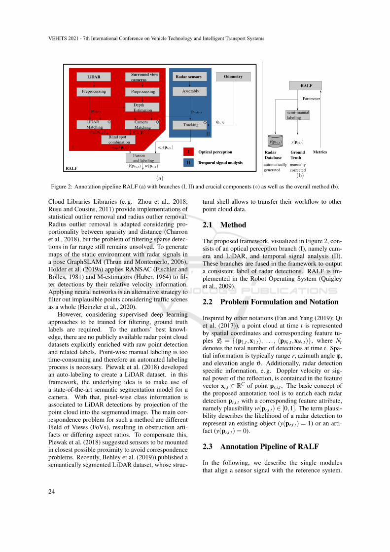
In contrast, we propose a generic method to au-tomatically label radar detections based on on-boardsensors denoted as Radar Sensor Artifact LabelingFramework (RALF). RALF enables a competitive,unbiased, and efficient data-enrichment pipeline asan automated process to generate consistent radardatasets including knowledge covering plausibility ofradar raw detections, see Figure 1. Inspired by Piewaket al. (2018), RALF applies the benefits of cross-modal sensors and is a composition of two parallelsignal processing pipelines as illustrated in Figure 2:Optical perception (I), namely camera and LiDAR aswell as temporal signal analysis (II) of radar detec-tions. Initially, false labeled predictions of RALFcan be manually corrected, so one obtains herebya ground truth dataset. This enables evaluation ofRALF, optimization of its parameters, and finally un-supervised label predictions on radar raw detections.

Our key contributions are the following:

1. An evaluation method to rate radar detectionsbased on their existence plausibility using LiDARand a monocular surround view camera system.

2. A strategy to take the transient signal course intoaccount with respect to the detection plausibility.

3. An automated annotation framework (RALF) togenerate binary labels for each element of radarpoint cloud data describing its plausibility of ex-istence, see Figure 1.

4. A simple semi-manual annotation procedure us-ing predictions of RALF to evaluate the labeling

results, optimize the annotation pipeline, and gen-erate a reviewed radar dataset.

2 RELATED WORK

To deploy radar signals more easily in AD and ADASapplications, raw signal de-noising1 is compulsory.Radar de-noising can be done on different abstrac-tion levels, at lowest on received reflections in thetime or frequency domain (e. g. Rock et al. (2019)).At a higher signal processing level of detections in3D space, point cloud operations offer rich oppor-tunities. For instance, point cloud representationsprofit from the importance of LiDAR sensors and theavailability of many famous public LiDAR datasets(Sun et al. (2020); Caesar et al. (2020); Geiger et al.(2013)) in company with many powerful point cloudprocessing libraries such as pcl (Rusu and Cousins,2011) or open3D (Zhou et al., 2018). Transferredto sparse LiDAR point cloud applications, Charronet al. (2018) discussed shortcomings of standard fil-ter methods (e. g. image filtering approaches to failat sparse point cloud de-noising). DBSCAN (Esteret al., 1996) is an adequate measure to cope withsparse noisy point clouds (Kellner et al., 2012). Point

1We use the term de-noising to distinguish between plausi-ble radar detections and artifacts, denoting no limitationonly to noise in the classical sense. Our understandingof radar artifacts is based on the work of Holder et al.(2019b). To name an example, an artifact could be a mir-ror reflection, a target could be a typical object like a car,building or poles.

Radar Artifact Labeling Framework (RALF): Method for Plausible Radar Detections in Datasets

23

Preprocessing

LiDAR Surround viewcameras

Preprocessing

LiDARMatching

Fusionand labeling

Assembly

Tracking

Radar sensors

Optical perception

Temporal signal analysis

Odometry

RALF

Parameter

manuallycorrected

automaticallygenerated

RadarDatabase

GroundTruth

Metrics

RALF

Blind spotcombination

CameraMatching

DepthEstimation semi-manual

labelingψt ,vt

pradar,tplidar,t

wlm(pr,i,t ) wcm(pr,i,t )

wopt (pr,i,t ) wtr(pr,i,t )

y(pr,i,t ) w(pr,i,t )

y(pr,i,t ) y(pr,i,t )

Temporal signal analysis

Figure 2: Annotation pipeline RALF (a) with branches (I, II) and crucial components (�) as well as the overall method (b).

Cloud Libraries Libraries (e. g. Zhou et al., 2018;Rusu and Cousins, 2011) provide implementations ofstatistical outlier removal and radius outlier removal.Radius outlier removal is adapted considering pro-portionality between sparsity and distance (Charronet al., 2018), but the problem of filtering sparse detec-tions in far range still remains unsolved. To generatemaps of the static environment with radar signals ina pose GraphSLAM (Thrun and Montemerlo, 2006),Holder et al. (2019a) applies RANSAC (Fischler andBolles, 1981) and M-estimators (Huber, 1964) to fil-ter detections by their relative velocity information.Applying neural networks is an alternative strategy tofilter out implausible points considering traffic scenesas a whole (Heinzler et al., 2020).

However, considering supervised deep learningapproaches to be trained for filtering, ground truthlabels are required. To the authors’ best knowl-edge, there are no publicly available radar point clouddatasets explicitly enriched with raw point detectionand related labels. Point-wise manual labeling is tootime-consuming and therefore an automated labelingprocess is necessary. Piewak et al. (2018) developedan auto-labeling to create a LiDAR dataset. in thisframework, the underlying idea is to make use ofa state-of-the-art semantic segmentation model for acamera. With that, pixel-wise class information isassociated to LiDAR detections by projection of thepoint cloud into the segmented image. The main cor-respondence problem for such a method are differentField of Views (FoVs), resulting in obstruction arti-facts or differing aspect ratios. To compensate this,Piewak et al. (2018) suggested sensors to be mountedin closest possible proximity to avoid correspondenceproblems. Recently, Behley et al. (2019)) published asemantically segmented LiDAR dataset, whose struc-

tural shell allows to transfer their workflow to otherpoint cloud data.

2.1 Method

The proposed framework, visualized in Figure 2, con-sists of an optical perception branch (I), namely cam-era and LiDAR, and temporal signal analysis (II).These branches are fused in the framework to outputa consistent label of radar detections. RALF is im-plemented in the Robot Operating System (Quigleyet al., 2009).

2.2 Problem Formulation and Notation

Inspired by other notations (Fan and Yang (2019); Qiet al. (2017)), a point cloud at time t is representedby spatial coordinates and corresponding feature tu-ples Pt = {(p1,t ,x1,t), . . . , (pNt ,t ,xNt ,t)}, where Ntdenotes the total number of detections at time t. Spa-tial information is typically range r, azimuth angle ϕ,and elevation angle ϑ. Additionally, radar detectionspecific information, e. g. Doppler velocity or sig-nal power of the reflection, is contained in the featurevector xi,t ∈ RC of point pr,i,t . The basic concept ofthe proposed annotation tool is to enrich each radardetection pr,i,t with a corresponding feature attribute,namely plausibility w(pr,i,t) ∈ [0,1]. The term plausi-bility describes the likelihood of a radar detection torepresent an existing object (y(pr,i,t) = 1) or an arti-fact (y(pr,i,t) = 0).

2.3 Annotation Pipeline of RALF

In the following, we describe the single modulesthat align a sensor signal with the reference system.

VEHITS 2021 - 7th International Conference on Vehicle Technology and Intelligent Transport Systems

24

Algorithm 1: LiDAR matching.

Require: Pradar,t ,Plidar,tEnsure: wlm(pr,i,t)

for it = 1, . . .Nradar,t doq← K-NN(Plidar,t , pi,t , K)d← 0for l = 1, . . .K do

px,l,t , py,l,t , pz,l,t ← Plidar,t .get point(q [l])rl,t ,ϕl,t ,ϑl,t ← Plidar,t .get features(q [l])σd,i,l← MODEL(rr,i,t ,ϕr,i,t ,ϑr,i,t ,rl,t ,ϕl,t ,ϑl,t )

d← d +

√∆p2

x,t+∆p2y,t+∆p2

z,t

σ2d,i,l+ε

end forwlm(pr,i,t)← exp(−βlm

dK )

end for

To enable comparison of multi-modal sensors, timesynchronization (Faust and Pradeep, 2020) and co-ordinate transformation (Dillmann and Huck, 2013)into a common reference coordinate system (see Sec-tion 3.1) are necessary.

LiDAR Matching. This module aligns radar detec-tions with raw LiDAR reflections as described in Al-gorithm 1. The LiDAR reflections are assumed tobe reliable and unbiased. Based on a flexible dis-tance measure, plausibility of radar detections is de-termined. The hypothesis of matching reliable radardetections with LiDAR signals in a single point inspace does not hold in general. LiDAR signals are re-flected on object shells, while radar waves might alsopenetrate objects. Thus, some assumptions and relax-ations are necessary in Algorithm 1. We assume forthe assessment no negative weather impact on LiDARsignals and comparable reflection modalities. Fur-thermore, since radar floor detections are mostly im-plausible, we estimate the LiDAR point cloud groundplane parameters via RANSAC (Fischler and Bolles,1981) and filter out corresponding radar points. Ap-plying a k-Nearest Neighbor (k-NN) clustering (Zhouet al. (2018); Rusu and Cousins (2011)) in Algo-rithm 1, each radar detection pr,i,t of the radar pointcloud Pradar,t , is associated with its K nearest neigh-bors of the LiDAR scan Plidar,t . Notice that values ofK greater than one improve the robustness due to lesssparsity in LiDAR scans. Measurement equations

hx = rr,i cosϑr,i cosϕr,i +vxradar

−(rl cosϑl cosϕl +vxlidar), (1)

hy = rr,i cosϑr,i sinϕr,i +vyradar

−(rl cosϑl sinϕl +vylidar), (2)

hz = rr,i sinϑr,i +vzradar− (rl sinϑl +

vzlidar) (3)

are introduced as components of L2 norm d inCartesian coordinates. Radar (rr,i,ϕr,i,ϑr,i) and Li-DAR detections (rl ,ϕl ,ϑl) are initially measuredin the local sphere coordinate system. Con-stant translation offsets (vxradar,

vyradar,vzradar) and

(vxlidar,vylidar,

vzlidar) relate the local sensor originsto the vehicle coordinate system. Assuming indepen-dence between uncertainties of radar coordinate mea-surements (σr,radar,σϕ,radar,σϕ,radar) as well as Time-of-Flight LiDAR uncertainty (σr,lidar), error propaga-tion in Cartesian space can be obtained by

σ2d,i,l =

(∂d

∂rr,i

)2

σ2r,radar +

(∂d

∂ϕr,i

)2

σ2ϕ,radar

+

(∂d

∂ϑr,i

)2

σ2ϑ,radar +

(∂d∂rl

)2

σ2r,lidar

(4)

denoted as MODEL in Algorithm 1. Rescaling the mis-match in each coordinate dimension enables the re-quired flexibility in the LiDAR matching module. Toensure wlm(pr,i,t) ∈ [0,1] and also increase resolutionin small mismatches d, an exponential decay functionwith a tuning parameter βlm ∈ R+ is applied subse-quently.

Camera Matching. Holding for general mount-ings, we undistort the raw images and apply a per-spective transformation to obtain a straight view, Fig-ures 3 and 4. We derive the modified intrinsic cameramatrix A ∈ R3×3 for the undistorted image (Scara-muzza et al., 2006). To match 3D radar point cloudswith camera perception, a dense optical representa-tion is necessary.

Structure-from-Motion (SfM) (Mur-Artal et al.,2015) on monocular images reconstructs sparsely.Reconstruction is often incomparable to radar, due tofew salient features in poorly structured parking sce-narios e. g. plain walls in close proximity. Moreover,initialization issues in low-speed situations naturallydegrades SfM to be reliable for parking.

Hence, we apply a pre-trained version of Di-verseDepth (Yin et al., 2020) on pre-processed imagesto obtain relative depth image estimations. Thanksto the diverse training set and the resulting general-ization, it outperforms other estimators trained onlyfor front cameras on datasets such as KITTI (Geigeret al., 2013). Thus, it is applicable to generic viewsand cameras. To match the depth image estima-tions to a metric scale, LiDAR detections in the over-lapping FoV are projected into each camera frameconsidering intrinsic and extrinsic camera parameters(world2cam). The projected LiDAR reflections serveas sparse sampling points from which the depth im-age pixels are metrically rescaled. Local scaling fac-


25

Figure 3: Camera matching pipeline.

Figure 4: Preprocessed surround view camera in examplescene.

Figure 5: Blind spot LiDAR.

tors outperform single scaling factors from robust pa-rameter estimation (Fischler and Bolles (1981); Hu-ber (1964)) at metric rescaling. Equidistant sam-ples of depth image pixels are point-wisely calibratedwith corresponding LiDAR points via KNN. Figure 3shows how the calibrated depth is projected back toworld coordinates by the (cam2world) function. Af-terwards, the association to radar detections analo-gously follows Algorithm 1, but considers the uncer-tainty of the depth estimation and its propagation inCartesian coordinates.

Though, being aware of camera failure modes,potential model failures requests for manual reviewof automated RALF results. Measuring inconsisten-cies between camera depth estimation and extrapo-lated LiDAR detections or LiDAR depth in overlap-ping FoVs, indicate potential failures.

Blind Spot Combination. In the experimentalsetup, described in Section 3.1, optical perception uti-lizing a single, centrally mounted LiDAR sensor lacksto cover the whole radar FoV as illustrated in Figure 5.The set

Vbs,l =

{pi = (pr,x,i, pr,y,i, pr,z,i)

> ∈ R3 | pr,z,i

∈ [0,zl]∧√

(pr,x,i− xl)2 + p2r,y,i ≤

zl− pr,z,i

tanαl

} (5)

describes the LiDAR blindspot resulting fromschematic mounting parameters (yl = 0,zl > 0) andopening angle αl greater than zero. Considering thedifferent FoVs,

wopt(pr,i,t) =

{wcm(pr,i,t) pr,i,t ∈Vbs,l

wlm(pr,i,t) otherwise(6)

summarizes the plausibility of the optical perceptionbranch (I). Far range detection relies only on LiDARsensing, while only cameras sense the nearfield. Atoverlapping intermediate sensing ranges, both rank-ings from camera and LiDAR scan are availableinstead of being mutually exclusive. Experimentsyielded more accurate results for this region by pre-ferring LiDAR over camera instead of a compromiseof both sensor impressions.

Tracking. Assuming Poisson noise (Buhren andYang, 2007) on radar detections, it is probable thatreal existing objects in space form hot spots over con-secutive radar measurement frames, whereas clutterand noise is almost randomly distributed. Since la-beling is not necessarily a real-time capable onlineprocess, one radar point cloud Pradar,tk at tk forms thereference to evaluate spatial reoccurence of detectionsin radar scan sequences. Therefore, a batch of nb ∈ Nearlier and subsequent radar point clouds are bufferedaround the reference radar scan at time tk. Consider-ing low speed planar driving maneuvers, applying akinematic single-track model based on wheel odome-try is valid (Werling, 2017). Based on the measuredyaw rate ψ, the longitudinal vehicle velocity v, andthe known time difference ∆t between radar scan k+1


26

Figure 6: Reliabilty scaling.

and k, the vehicle state is approximated by(xv,yv,zv,ψ

)>k+1 =

(xv,yv,zv,ψ

)>k

+∆t ·(v cosψ,v sinψ,0, ψ

)>k .

(7)

Considering Equation (7) and rotation matrix Rz,ψ,containing yaw angle ψ, allows ego-motion compen-sation for each point i of the buffered radar pointclouds Pradar,tk+ j for j ∈ {−nb, . . . ,−1, 1, . . . ,nb} tothe reference cloud Pradar,tk . Each point

pr,i,tk+ j = R−1z,ψk

((xv,yv,zv

)>k+ j−

(xv,yv,zv

)>k

)+ Rz,ψk+ j−ψk pr,i,tk+ j

(8)

represents the spatial representation of a consecutiveradar scan after ego-motion compensation to the ref-erence radar scan at time step tk. Enabling tempo-ral tracking and consistency checks on the scans, nbshould be chosen regarding the sensing cycle time.Assuming to analyze mainly static objects, Equa-tion (8) is valid. To describe dynamic objects, Equa-tion (8) has to be extended considering Doppler veloc-ity and local spherical coordinates of each detection.By taking error propagation in the resulting measure-ment equations into account, different uncertainty di-mensions are applicable. We apply spatial uncertaintyas in Equation (4). The analysis of nb scans resultin a batch of distance measures d j. Simple averag-ing fails due to corner-case situations in which po-tentially promising detections remain undetected inshort sequences. Hence, sorting d j in ascending or-der and summing the sorted distances, weighted by adecreasing coefficient with increasing position, yieldspromising results.

Fusion and Final Labeling. The outputs of opticalperception and tracking are combined with a setup-specific sensor a-priori information γs(ϕ)∈ [1,∞), seeFigure 6. Since radar sensors are often covered be-hind bumpers, inhomogenous measurement accura-cies γs(ϕr,i,t) arise over the azimuth range ϕ, see Fig-ure 6. The a-priori known sensor specifics are mod-eled by the denominator in Equation (9).

The tuning parameter α ∈ [0,1] prioritizes be-tween the tracking and optical perception module,formalized as first term w(pr,i,t) of the Heaviside

Figure 7: Parameter selection in RALF for branch weightsα and plausibility threshold w0.

function H : R → {0,1} argument in Equation (9).The final binary labels to discriminate artifacts (y= 0)from promising detections (y = 1) are obtained by

y(pr,i,t) = H(w(pr,i,t)−w0

)= H

(α wopt(pr,i,t)+(1−α) wtr(pr,i,t)

γs(ϕr,i,t)−w0

),

(9)

where w0 ∈ [0,1] ia a threshold on the prioritizedoptical perception and tracking results.

2.4 Use-case Specific Labeling Policy

Motives for labeling a dataset might vary with the de-sired application purpose, along with conflicting pa-rameter selection for some use cases. Our frame-work parameters allow to tune the automated label-ing. High α = 1 suppresses radar detections withoutLiDAR detections or camera detections in their neigh-borhood, while low α= 0 emphasizes temporal track-ing over the visual alignment, see Figure 7.

Low α = 0 settings include plausible detections tooccur behind LiDAR reflections, e. g. reflecting frominside a building. But, plausible radar detections arerequired to be locally consistent over several scans.On the upper bound α = 1, the temporal tracking con-sistency constraint vanishes its influence on the plau-sible detections, resulting in an optical filtering. Forinstance, plausibility is rated high around LiDAR andcamera perception. Examples for the relevance oftemporal tracking might be the localization on radar.To recognize a known passage, the scene signatureand temporal sequence of radar scans might be muchmore important than a de-noised representation of ascene. The other extreme might be the use-case of se-mantic segmentation on radar point clouds where oneis interested in the nearest and shell describing radarreflections, omitting reflections from the inside of ob-jects. Parameter w0 acts as threshold margin on theplausibility.

RALF parameters α,βlm,βcm,βtr,nb and K can betuned by manual inspection and according to the de-sired use-case. The error metrics in Equation (10)-(14), introduced in the Appendix, help to finetune theparametrization as visualized in Figure 2(b).

Optimizing RALF subsequentially leads to moreaccurate predictions and decaying manual label cor-rections. However, proper initial parameters and hav-


27

Figure 8: Sensor setup.

Table 1: Sensor setup details.

Name Details

Camera 4 x Monocular surround view camera(series equipment)

LiDAR Rotating Time-of-Flight LiDAR(centrally roof-mounted, 40 channel)

Radar 77 GHz FMCW Radar(FoV: 160 degree h. , ±10 degree v.)

ing a manageable parameter space is essential. Af-ter this fine-tuning step, no further manual parameterinspection of RALF is necessary. The automaticallypredicted radar labels can be directly used to annotatethe dataset.

We tune the desired performance to achieve anoverestimating function. Manual correction benefitsof coarser estimates that can be tailored to groundtruth labels, whereas extension of bounds requires se-vere interference with clutter classifications. Hence,in Table 3, we aim for high Recall values while al-lowing lower Accuracy.

2.5 Error Evaluation

An error measure expressing the quality of the au-tomated labeling is essential in two aspects, namelyto check if the annotation pipeline is appropriate ingeneral and to optimize its parameters. Since thispaper proposes a method to generate plausibility ofradar detections, it is challenging to describe a generalmeasure that evaluates the results. Without groundtruth labels, only indirect metrics are possible. Forinstance distinctiveness, expressed as difference be-tween means of weights per class in combination withbalance of class members. However, several cases canbe constructed in which this indirect metric misleads.Therefore, we semi-manually labeled a set of M = 11different scans assisted by RALF to correctly evaluatethe results, see Section 3.2 and Table 3.

3 EXPERIMENTS

In the first section, we describe the hardware sensorsetup for the real world tests. After that, we discuss

how the labeling policy depends on the use-case, andfinally evaluate the results of the real world test.

3.1 Sensor Setup and ExperimentalDesign

The vehicle test setup is depicted in Figure 8 andsensor set details are found in Table 1. We evalu-ate the radar perception for a radar-mapping park-ing functionality. Eleven reference test tracks (e. g.urban area, small village, parking lot and industrialpark) were considered and are depicted in the Ap-pendix. To ensure a balanced, heterogeneous dataset,they contain parking cars, vegetation, building struc-tures as well as a combination of car parks (open airand roofed). Vehicle velocity v below 10kph duringthe perception of the test track environment ensureslarge overlapping areas in consecutive radar scans.

3.2 Semi-manual Labeling usingPredictions of RALF

We use the predictions of RALF as a first labelingguess for which humans are responsible to correctfalse positives and false negatives. To ensure accu-rate corrections of RALF predictions, we visualizeboth radar and LiDAR clouds in a common referenceframe and consider all parallel cameras to achieveground truth data semi-manually.

Table 2: Test set class balance over N = 2704 radar scans.

ΣN ∅N(y=1)∅N

∅N(y=0)∅N

3 288 803 21.55 % 78.45 %

We base the evaluation on a dataset of eleven inde-pendent test tracks for which we compare the RALFlabels versus the manually corrected results. Con-taining two classes, the overall class balance of thedataset is 78.45% clutter (2 580 066 radar points)against 21.55% plausible detections (708 737 radarpoints). Details can be found in Table 3. Additionalimagery info and dataset statistics are found in the ap-pendix. Please note, following our manual correc-tion policy, radar reflections of buildings are reducedto their facade reflections. Intra-building reflectionsare re-labeled as clutter although the detections mightcorrectly result from inner structures. This resultsin heavily distorted average IoU values of plausibledetections ranging from 36.7% to 60.9%, Table 3.This assumption is essential for re-labeling and man-ual evaluation of plausible detections. Intra-structuralreflections are hard to rate in terms of plausibility. Be-


28

Table 3: Test dataset of M = 11 sequences.

ID ∅N ∅Acc ∅Precision ∅Recall F1 plausible ∅IoU IoU plausible IoU artifact

Σ 2704 0.873 0.826 0.779 0.675 0.682 0.510 0.854

00 245 0.848 0.833 0.793 0.722 0.687 0.565 0.81001 290 0.883 0.796 0.781 0.646 0.673 0.477 0.86902 101 0.878 0.839 0.822 0.740 0.720 0.588 0.85203 400 0.885 0.706 0.761 0.622 0.662 0.451 0.87304 334 0.927 0.863 0.859 0.765 0.768 0.620 0.91705 163 0.910 0.869 0.845 0.757 0.752 0.609 0.89506 170 0.776 0.771 0.678 0.537 0.554 0.367 0.74207 422 0.860 0.808 0.739 0.616 0.644 0.445 0.82408 265 0.850 0.759 0.771 0.622 0.640 0.451 0.82909 82 0.845 0.813 0.776 0.684 0.667 0.520 0.81410 232 0.874 0.844 0.798 0.715 0.703 0.556 0.850

sides, in a transportation application, the sensory hulldetection of objects needs to be reliable.

Using the data format of SemanticKitti dataset forLiDAR point clouds (Behley et al., 2019), the eval-uation of reliable radar detections orientates on thefollowing clusters: human, vehicle, construction,vegetation, poles. Our proposed consolidation oforiginal SemanticKITTI classes to a reduced numberof clusters is found in the Appendix, see Table 5. Es-pecially the vegetation class imposes labeling con-sistency. E. g. grass surfaces can be treated as relevantif the discrimination of insignificant reflections fromground seems possible. On the other hand, grass andother vegetation are source of cluttered, temporallyand often also spatially unpredictable reflections.

Different labeling philosophies impose the neces-sity of a consistent labeling policy. In the discusseddataset of this work, we emphasize on grass surfacesas plausible radar reflections in order to discriminategreen space from road surface. Stuctural reflectionsare labeled based on facade reflections, while intra-vehicle detections are permitted as relevant. Pleasenote, road surface reflections are labeled as clutter.Table 2 shows the class distribution of the labeledreference test of M = 11 sequences with in average∅N = 1216 radar detections for evaluation in Sec-tion 3.3. Inspecting Table 2, please note, that thedataset has imbalanced classes, so a detection is morelikely to be an artifact.

3.3 Results

The following section discusses the results on realworld data and includes an evaluation.

Monocular Depth Estimation. Figure 9 illustratesthat the pre-trained depth estimation network providesfair results on pre-processed surround view cameras.

Figure 9: Input image (a) for depth estimation (b) with high-lighted objects; depth encoded by increasing brightness (b).

Figure 10: Birds-eye-view on example a scene with coloredOpenStreetMap data (OpenStreetMap Contributors, 2017).Comparison accumulated radar scans (black points): (a) alldetections (b) plausible RALF detections (y(pi,t) = 1) with-out relabeling.

Key contribution to achieve reasonable results on fish-eye images without retraining are a perspective trans-formation and undistortion. However, in very similarscenes as shown in Figure 9, it is challenging to esti-mate the true relative depth. By using local LiDARscales as we propose, this issue can be solved ele-gantly and thus an overlap of LiDAR and camera FoVis a helpful benefit. Moreover, the results in Figure 3and Figure 9 show that the depth estimation networkgeneralizes to other views and scenes.

Qualitative Comparison Raw vs. Labeled Data.Figure 10 illustrates an example scene. The results ofRALF in this scene compared to unlabeled raw dataare shown in Figures 4 and 10. Scene understandingis considerably facilitated.

Quantitative Evaluation. We use the prefacedmanually labeled test set to evaluate the proposed


29

Table 4: Confusion matrix on dataset with ΣN detections.

y = 1 y = 0

y = 1 2 432 440 268 869y = 0 157 076 430 418

pipeline. The confusion matrix of the dataset arefound in Table 4. By achieving a mean error L =12.95 %= (1-Accuracy) on the dataset, we demonstrate the ca-pability of the proposed pipeline to generate mean-ingful labels on real world test tracks. Please notethe beneficial property of overestimation. Comparingan average Recall of 77.9 % to an average Precision82.6 % in Table 3, there is no preferred error in the la-beling pipeline of RALF. Since RALF can be param-eterized, increasing Recall and decreasing Precisionor vice versa is possible by tuning the introduced pa-rameters w0 and α. Inspecting the differences of theperformance per sequence, sequence 06 is exemplaryfor the lower performance, while sequence 04 per-forms best. Interestingly, these two sequences over-lap partly. Sequence 06, including an exit of a narrowgarage, poses difficulties in the close surrounding ofthe car, which explains the performance decrease.

Robustness. Errors can be provoked by camera ex-ceptions (lens flare, darkness, etc.) and assumptionviolations. Near-field reconstruction results sufferin cases when ground and floor-standing objects inlow height can not distinguished accurately, yieldingvague near-field labels. Furthermore, in non-planarenvironments containing e. g. ascents, the planar Li-DAR floor extraction misleads. This causes RALF tomislabel radar floor detections. Moreover, the track-ing module suffers at violated kinematic single-trackmodel assumptions.

4 CONCLUSION

We propose RALF, a method to rate radar detectionsconcerning their plausibility by using optical percep-tion and analyzing transient radar signal course. Bya combination of LiDAR, surround view cameras,and DiverseDepth, we generate a 360 degree per-ception in near- and far-field. DiverseDepth yieldsa dense depth estimation, outperforming SfM ap-proaches. Monitored via LiDAR, failure modes canbe detected. Since considering model and sensor un-certainties respectively, a flexible comparison usingdifferent sensors is possible. From the optical per-ception branch, radar detections can be enriched byLiDAR or camera information as a side effect. Such

a feature is useful for developing applications usingannotated radar datasets. To evaluate RALF and fine-tune its parameters, RALF predictions can be semi-manually corrected to ground truth labels. Recordedvehicle measurements on real-world test tracks yieldan average Accuracy of 87.3% at average Precision of82.6% of the proposed labeling method, though satis-fying de-noising capabilities. The evaluation revealspositive effects of an overestimating labeling perfor-mance. Time and effort for labeling are reduced sig-nificantly. As side notice, the labeling policy is cou-pled with the desired use-case and evaluation metricswhich may differentiate. We plan to extend the workon the framework towards semantic labeling.

ACKNOWLEDGEMENTS

We thank Marc Muntzinger form Car.Software Org,Marc Runft from IAV, and Michael Frey from Insti-tute of Vehicle System Technology (Karlsruhe Insti-tute of Technology) for their valuable input and thediscussions. Furthermore, we would like to thank thewhole team at the Innovation Campus from PorscheAG. Moreover, we thank all reviewers whose com-ments have greatly improved this contribution.

REFERENCES

Behley, J., Garbade, M., Milioto, A., Quenzel, J., Behnke,S., Stachniss, C., and Gall, J. (2019). Semantickitti:A dataset for semantic scene understanding of lidarsequences. In 2019 IEEE/CVF International Confer-ence on Computer Vision, ICCV 2019, Seoul, Korea(South), October 27 – November 2, 2019, pages 9296–9306. IEEE.

Buhren, M. and Yang, B. (2007). Simulation of automotiveradar target lists considering clutter and limited reso-lution. In Proc. of International Radar Symposium,pages 195–200.

Caesar, H., Bankiti, V., Lang, A. H., Vora, S., Liong, V. E.,Xu, Q., Krishnan, A., Pan, Y., Baldan, G., and Bei-jbom, O. (2020). nuscenes: A multimodal dataset forautonomous driving. In 2020 IEEE/CVF Conferenceon Computer Vision and Pattern Recognition, CVPR2020, Seattle, WA, USA, June 13-19, 2020, pages11618–11628. IEEE.

Charron, N., Phillips, S., and Waslander, S. L. (2018). De-noising of lidar point clouds corrupted by snowfall. In15th Conference on Computer and Robot Vision, CRV2018, Toronto, ON, Canada, May 8-10, 2018, pages254–261. IEEE Computer Society.

Dillmann, R. and Huck, M. (2013). Informationsverar-beitung in der Robotik, page 270. Springer-Lehrbuch.Springer Berlin Heidelberg.


30

Eriksson, L. H. and As, B. (1997). Automotiveradar for adaptive cruise control and collision warn-ing/avoidance. In Radar 97 (Conf. Publ. No. 449),pages 16–20.

Ester, M., Kriegel, H., Sander, J., and Xu, X. (1996). Adensity-based algorithm for discovering clusters inlarge spatial databases with noise. In Simoudis, E.,Han, J., and Fayyad, U. M., editors, Proceedings of theSecond International Conference on Knowledge Dis-covery and Data Mining (KDD-96), Portland, Ore-gon, USA, pages 226–231. AAAI Press.

Everingham, M., Eslami, S. M. A., Gool, L. V., Williams,C. K. I., Winn, J. M., and Zisserman, A. (2015). Thepascal visual object classes challenge: A retrospec-tive. Int. J. Comput. Vis., 111(1):98–136.

Fan, H. and Yang, Y. (2019). PointRNN: Point recurrentneural network for moving point cloud processing.pre-print, arXiv:1910.08287.

Faust, J. and Pradeep, V. (2020). Message filter: Ap-proximate time. http://wiki.ros.org/message filters/ApproximateTime. Accessed: 2020-04-30.

Feng, D., Haase-Schutz, C., Rosenbaum, L., Hertlein,H., Glaser, C., Timm, F., Wiesbeck, W., and Diet-mayer, K. (2020). Deep multi-modal object detectionand semantic segmentation for autonomous driving:Datasets, methods, and challenges. IEEE Transac-tions on Intelligent Transportation Systems, PP:1–20.

Fischler, M. A. and Bolles, R. C. (1981). Random sampleconsensus: A paradigm for model fitting with appli-cations to image analysis and automated cartography.Commun. ACM, 24(6):381–395.

Geiger, A., Lenz, P., Stiller, C., and Urtasun, R. (2013).Vision meets robotics: The KITTI dataset. Int. J.Robotics Res., 32(11):1231–1237.

Heinzler, R., Piewak, F., Schindler, P., and Stork, W. (2020).CNN-based LiDAR point cloud de-noising in adverseweather. IEEE Robotics Autom. Lett., 5(2):2514–2521.

Holder, M., Hellwig, S., and Winner, H. (2019a). Real-timepose graph SLAM based on radar. In 2019 IEEE In-telligent Vehicles Symposium, IV 2019, Paris, France,June 9–12, 2019, pages 1145–1151. IEEE.

Holder, M., Linnhoff, C., Rosenberger, P., Popp, C., andWinner, H. (2019b). Modeling and simulation of radarsensor artifacts for virtual testing of autonomous driv-ing. In 9. Tagung Automatisiertes Fahren.

Huber, P. J. (1964). Robust estimation of a location param-eter. Ann. Math. Statist., 35(1):73–101.

Kellner, D., Klappstein, J., and Dietmayer, K. (2012). Grid-based DBSCAN for clustering extended objects inradar data. In 2012 IEEE Intelligent Vehicles Sympo-sium, IV 2012, Alcal de Henares, Madrid, Spain, June3–7, 2012, pages 365–370. IEEE.

Meyer, M. and Kuschk, G. (2019). Automotive radardataset for deep learning based 3d object detection.In 2019 16th European Radar Conference (EuRAD),pages 129–132.

Mur-Artal, R., Montiel, J. M. M., and Tardos, J. D. (2015).ORB-SLAM: A versatile and accurate monocular

SLAM system. IEEE Trans. Robotics, 31(5):1147–1163.

OpenStreetMap Contributors (2017). Planet dump re-trieved from https://planet.osm.org. https://www.openstreetmap.org.

Piewak, F., Pinggera, P., Schafer, M., Peter, D., Schwarz,B., Schneider, N., Enzweiler, M., Pfeiffer, D., andZollner, J. M. (2018). Boosting LiDAR-based seman-tic labeling by cross-modal training data generation.In Leal-Taixe, L. and Roth, S., editors, Computer Vi-sion - ECCV 2018 Workshops - Munich, Germany,September 8-14, 2018, Proceedings, Part VI, volume11134 of Lecture Notes in Computer Science, pages497–513. Springer.

Qi, C. R., Yi, L., Su, H., and Guibas, L. J. (2017). Point-net++: Deep hierarchical feature learning on point setsin a metric space. In Guyon, I., von Luxburg, U., Ben-gio, S., Wallach, H. M., Fergus, R., Vishwanathan, S.V. N., and Garnett, R., editors, Advances in Neural In-formation Processing Systems 30: Annual Conferenceon Neural Information Processing Systems 2017, 4-9December 2017, Long Beach, CA, USA, pages 5099–5108.

Quigley, M., Conley, K., Gerkey, B., Faust, J., Foote, T.,Leibs, J., Wheeler, R., and Ng, A. (2009). ROS: Anopen-source robot operating system. volume 3.

Rock, J., Toth, M., Messner, E., Meissner, P., and Pernkopf,F. (2019). Complex signal denoising and interferencemitigation for automotive radar using convolutionalneural networks. In 22th International Conferenceon Information Fusion, FUSION 2019, Ottawa, ON,Canada, July 2-5, 2019, pages 1–8. IEEE.

Rusu, R. B. and Cousins, S. (2011). 3d is here: Pointcloud library (PCL). In IEEE International Confer-ence on Robotics and Automation, ICRA 2011, Shang-hai, China, 9-13 May 2011. IEEE.

Scaramuzza, D., Martinelli, A., and Siegwart, R. (2006).A toolbox for easily calibrating omnidirectional cam-eras. In 2006 IEEE/RSJ International Conference onIntelligent Robots and Systems, IROS 2006, October9-15, 2006, Beijing, China, pages 5695–5701. IEEE.

Sun, P., Kretzschmar, H., Dotiwalla, X., Chouard, A., Pat-naik, V., Tsui, P., Guo, J., Zhou, Y., Chai, Y., Caine,B., Vasudevan, V., Han, W., Ngiam, J., Zhao, H., Tim-ofeev, A., Ettinger, S., Krivokon, M., Gao, A., Joshi,A., Zhang, Y., Shlens, J., Chen, Z., and Anguelov,D. (2020). Scalability in perception for autonomousdriving: Waymo open dataset. In 2020 IEEE/CVFConference on Computer Vision and Pattern Recogni-tion, CVPR 2020, Seattle, WA, USA, June 13-19, 2020,pages 2443–2451. IEEE.

Thrun, S. and Montemerlo, M. (2006). The graph SLAMalgorithm with applications to large-scale mapping ofurban structures. Int. J. Robotics Res., 25(5–6):403–429.

Werling, M. (2017). Optimale aktive Fahreingriffe:Fur Sicherheits- und Komfortsysteme in Fahrzeugen,pages 89–90. De Gruyter Oldenbourg.

Yin, W., Wang, X., Shen, C., Liu, Y., Tian, Z., Xu, S., Sun,C., and Renyin, D. (2020). DiverseDepth: Affine-


31

invariant depth prediction using diverse data. pre-print, arXiv:2002.00569.

Yurtsever, E., Lambert, J., Carballo, A., and Takeda, K.(2020). A survey of autonomous driving: Commonpractices and emerging technologies. IEEE Access,8:58443–58469.

Zhou, Q., Park, J., and Koltun, V. (2018). Open3d: Amodern library for 3d data processing. pre-print,arXiv:1801.09847.

APPENDIX

Class Consolidation

The authors of SemanticKITTI (Behley et al., 2019)introduce a class structure in their work. To transferthis approach to radar detections, we propose a con-solidation of classes as found in Table 5.

Table 5: Proposed clustering of SemanticKITTIclasses (Behley et al., 2019) to determine radar arti-facts.

Cluster SemanticKITTI Classes

Vehicle car, bicycle, motorcycle, truck, other-vehicle, busHuman person, bicyclist, motorcyclistContruction building, fenceVegetation vegetation, trunk, terrainPoles pole, traffic sign, traffic lightArtifacts sky, road, parking, sidewalk, other-ground

Metrics

The applied metrics in Table 3 are formulated basedon the state-of-the art binary classification metricsTrue Positive (TP), False Positives (FP), True Neg-atives (TN), and False Negatives (FN).

Accuracy =T P+T N

T P+T N +FP+FN(10)

Precision =T P

T P+FP(11)

Recall =T P

T P+FN(12)

F1 =2 ·T P

2 ·T P+FP+FN(13)

The metric mean Intersection-over-Union (∅IoU) isbased on the mean Jaccard Index (Everingham et al.,2015) which is normalized over the classes C. TheIoU expresses the labeling performance class-wise.

∅IoU =1C

C

∑c=1

T Pc

T Pc +FPc +FNc(14)

Sequence Description

The set of sequences are shortly introduced for visualinspection and scene understanding.

Sequence 00. Urban crossing scene with build-ings, parked cars and vegetation in form of singulartrees along the road; see Figure 1.

Sequence 01. Scene on open space along parkedvehicles. Green area beside street and buildings inbackground; not displayed due to space limitation.

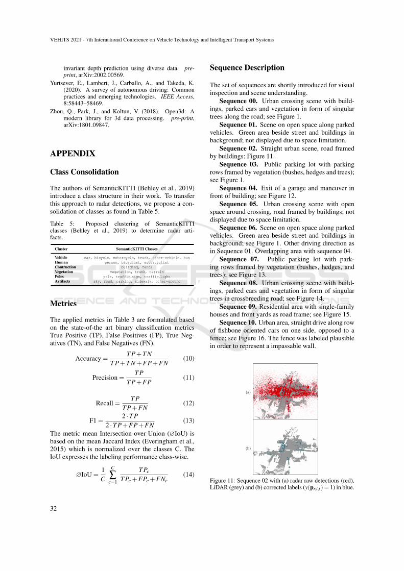
Sequence 02. Straight urban scene, road framedby buildings; Figure 11.

Sequence 03. Public parking lot with parkingrows framed by vegetation (bushes, hedges and trees);see Figure 1.

Sequence 04. Exit of a garage and maneuver infront of building; see Figure 12.

Sequence 05. Urban crossing scene with openspace around crossing, road framed by buildings; notdisplayed due to space limitation.

Sequence 06. Scene on open space along parkedvehicles. Green area beside street and buildings inbackground; see Figure 1. Other driving direction asin Sequence 01. Overlapping area with sequence 04.

Sequence 07. Public parking lot with park-ing rows framed by vegetation (bushes, hedges, andtrees); see Figure 13.

Sequence 08. Urban crossing scene with build-ings, parked cars and vegetation in form of singulartrees in crossbreeding road; see Figure 14.

Sequence 09. Residential area with single-familyhouses and front yards as road frame; see Figure 15.

Sequence 10. Urban area, straight drive along rowof fishbone oriented cars on one side, opposed to afence; see Figure 16. The fence was labeled plausiblein order to represent a impassable wall.

Figure 11: Sequence 02 with (a) radar raw detections (red),LiDAR (grey) and (b) corrected labels (y(pr,i,t) = 1) in blue.


32

Figure 12: Sequence 04; figure description is equal to Fig-ure 11.






33

Method for Plausible Radar Detections in Datasets - SciTePress

Documents

Transcript of Method for Plausible Radar Detections in Datasets - SciTePress