arX

iv:a

stro

-ph/

0010

197v

1 1

0 O

ct 2

000

Parent Stars of Extrasolar Planets VI: Abundance Analyses of 20

New Systems

Guillermo Gonzalez1, Chris Laws1, Sudhi Tyagi1, and B. E. Reddy2

Received ; accepted

Submitted to the Astronomical Journal

1University of Washington, Astronomy Department, Box 351580, Seattle, WA 98195

gonzalez@astro.washington.edu, laws@astro.washington.edu, styagi@u.washington.edu

2Department of Astronomy, University of Texas, Austin, TX 78713-1083

ereddy@shaka.as.utexas.edu

– 2 –

ABSTRACT

The results of new spectroscopic analyses of 20 recently reported extrasolar

planet parent stars are presented. The companion of one of these stars,

HD 10697, has recently been shown to have a mass in the brown dwarf regime;

we find [Fe/H] = +0.16 for it. For the remaining sample, we derive [Fe/H]

estimates ranging from −0.41 to +0.37, with an average value of +0.18 ± 0.19.

If we add the 13 stars included in the previous papers of this series and 6 other

stars with companions below the 11 MJup limit from the recent studies of Santos

et al., we derive 〈[Fe/H]〉 = +0.17 ± 0.20.

Among the youngest stars with planets with F or G0 spectral types, [Fe/H] is

systematically larger than young field stars of the same Galactocentric distance

by 0.15 to 0.20 dex. This confirms the recent finding of Laughlin that the most

massive stars with planets are systematically more metal rich than field stars

of the same mass. We interpret these trends as supporting a scenario in which

these stars accreted high-Z material after their convective envelopes shrunk to

near their present masses. Correcting these young star metallicities by 0.15 dex

still does not fully account for the difference in mean metallicity between the

field stars and the full parent stars sample.

The stars with planets appear to have smaller [Na/Fe], [Mg/Fe], and [Al/Fe]

values than field dwarfs of the same [Fe/H]. They do not appear to have

significantly different values of [O/Fe], [Si/Fe], [Ca/Fe], or [Ti/Fe], though. The

claim made in Paper V that stars with planets have low [C/Fe/] is found to be

spurious, due to unrecognized systematic differences among published studies.

When corrected for these differences, they instead display slightly enhanced

[C/Fe] (but not significantly so). If these abundance anomalies are due to the

accretion of high-Z matter, it must have a composition different from that of

– 3 –

the Earth.

Subject headings: planetary systems - stars: individual (HR 810, HD 1237, HD

10697, HD 12661, HD 16141, HD 37124, HD 38529, HD 46375, HD 52265, HD

75332, HD 89744, HD 92788, HD 130322, HD 134987, HD 168443, HD 177830,

HD 192263, HD 209458, HD 217014, HD 217107, HD 222582, BD -10 3166)

– 4 –

1. INTRODUCTION

In our continuing series on stars-with-planets (hereafter, SWPs), we have reported on

the results of our spectroscopic analyses of these stars (Gonzalez 1997, Paper I; Gonzalez

1998, Paper II; Gonzalez & Vanture 1998, Paper III; and Gonzalez et al. 1999, Paper IV;

Gonzalez & Laws 2000, Paper V). Other similar studies include Fuhrmann et al. (1997,

1998) and Santos et al. (2000b,c). The most significant finding so far has been the high

mean metallicity of SWPs, as a group, compared to the metallicity distribution of nearby

solar-type stars (Gonzalez 2000; Santos et al. 2000b,c).

Additional extrasolar planet candidates continue to be announced by planet hunting

groups using the Doppler method. We follow-up these annoucements with high resolution

spectroscopic observations as time and resources permit. Herein, we report on the results of

our abundance analyses of 20 new candidate SWPs. We compare our findings with those of

other recent similar studies, look for trends in the data suggested in previous studies, and

evaluate proposed mechanisms in light of the new dataset.

2. SAMPLE AND OBSERVATIONS

High-resolution, high S/N ratio spectra of 14 stars were obtained with the 2dcoude

echelle spectrograph at the McDonald observatory 2.7 m telescope using the same setup

as described in Paper V. Two stars difficult or impossible to observe from the northern

hemisphere, HR 810 and HD 1237, were observed on three nights with the CTIO 1.5 m with

the fiber fed echelle spectrograph. Observing them on multiple nights permits us to test for

possible variations in their temperatures over one stellar rotation period, given their youth.

Additional details of the spectra obtained at CTIO and McDonald, including a list of the

discovery papers, are presented in Table 1. Although it does not have a known planet,

– 5 –

we include HD 75332 in the program, since its physical parameters are similar to those of

the hotter SWPs. HD 75332 is also included in the field star abundance survey of Chen

et al. (2000), which we will be comparing to our results in Section 4.2.7. We also include

HD 217014 (51 Peg), even though it was already analyzed in Paper II, because: 1) the

new spectra are of much higher quality, and 2) it was included in the field star abundance

surveys of Edvardsson et al. (1993) and Tomkin et al. (1997).

High resolution spectra of nine stars (HD 12661, HD 16141, HD37124, HD 38529,

HD 46375, HD 52265, HD 92788, HD 177830, and BD -10 3166) 3 obtained with the HIRES

spectrograph on the Keck I were supplied to us by Geoff Marcy (see Paper IV for more

details on the instrument). The Keck spectra have the advantage of higher resolving power

and much weaker water vapor telluric lines, due to the altitude of the site. However, the

much smaller wavelength coverage of the Keck spectra results in a much shorter linelist for

us to work with.

The data reduction methods are the same as those employed in Paper V. Spectra of

hot stars with a high v sin i values were also obtained in order to divide out telluric lines in

the McDonald and CTIO spectra.

3. ANALYSIS

3.1. Spectroscopic Analysis

The present method of analysis is the same as that employed in Paper V, and therefore,

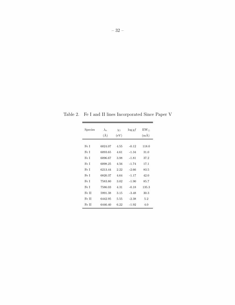
will not be described herein. We have added more Fe I, II lines to our linelist (Table 2).

3The discovery papers corresponding to these stars are: Butler et al. 2000; Fischer et al.

2000; Marcy et al. 2000; Sivan et al. 2000; Vogt et al. 2000.

– 6 –

Their gf -values were calculated from an inverted solar analysis using the Kurucz et al.

(1984) Solar Flux Atlas or our spectrum of Vesta (obtained with the McDonald 2.7 m). We

also added a new synthesized region: 9250 - 9270 A. This region contains one Mg I, two Fe I,

and three O I lines; only one of the O I triplet, 9266 A, is unblended in all our stars, but the

other two are usable in the warmer stars. The addition of a second Mg line to our linelist

helps greatly, because the 5711 line was the only one we had employed until now, and it is

not measurable in the cooler stars. We also added the O I triplet near 7770 A. Since these

lines are known to suffer from non-LTE effects, we have corrected the O abundances derived

from these lines using Takeda’s (1994) calculations. We list the individual EW values in

Tables 3 - 6 and present the adopted atmosphere parameters in Table 7. We list the [X/H]

values in Tables 8 - 12. We list in Table 13 Mg and O abundances (derived from the 9250

A region) for several stars studied in previous papers in our series.

Since we have not previously used the CTIO 1.5 m telescope for spectroscopic studies

of SWPs, we need an independent check on the zero point of the derived abundances for

HR810 and HD 1237. To accomplish this, we also obtained a spectrum of α Cen A with

this instrument. We derive the following values for Teff , log g, ξt, and [Fe/H]: 5774 ± 61 K,

4.22 ± 0.08, 0.90 ± 0.10, and +0.35 ± 0.05. This value of [Fe/H] is 0.10 dex larger than the

value derived by Neuforge-Verheecke & Magain (1997).

3.2. Derived Parameters

We have determined the masses and ages in the same way as in Paper V. Using the

Hipparcos parallaxes (ESA 1997) and the stellar evolutionary isochrones of Schaller et al.

(1992) and Schaerer et al. (1993), along with our spectroscopic Teff estimates, we have

– 7 –

derived masses, ages, and theoretical log g values (Table 14).4 BD-10 3166 is too distant for

a reliable parallax determination, so it is not included in the table.

Two stars, HD 37124 and HD 46375, give inconsistent results: they are located in a

region of the HR diagram where no ordinary stars are expected (they are too luminous

and/or too cool relative to even the oldest isochrones). One possible solution is to invoke an

unresolved companion of comparable luminosity. It is highly unlikely that the companion

is responsible for the observed radial velocity variations in each star, as that would require

them to be viewed very nearly pole-on, which is extremely improbable (Geoff Marcy, private

communication). It is more likely that the companions are sufficiently separated such that

they do not significantly affect the Doppler measurements on short timescales. Therefore,

we encourage that these two systems be searched for close stellar companions.

Several other stars, HD 1237, HD 130322, and HD 192263, are of too low a luminosity

to derive reliable ages, due to the convergence of the stellar evolutionary tracks at low

luminosities (see Figure 1). However, it is still possible to derive useful mass and log g

estimates for them. For those stars with theoretical log g estimates in Table 14, there is

generally good agreement with the spectroscopic values listed in Table 7.

4. DISCUSSION

4.1. Comparison with Other Studies

Several stars in the present study have been included in other recent spectroscopic

studies. Santos et al. (2000b,c) analyzed a total of 13 SWPs using a method patterned

4Note, the theoretical log g values are derived from theoretical stellar evolutionary

isochrones at the age which agrees with the observed Teff , Mv, and [Fe/H] values.

– 8 –

after that of Paper V. Two of their stars, HD 1237 and HD 52265, overlap with our present

sample (and one other, HD 75289, from Paper V). Their results for HD 75289 are nearly

identical to ours. Our McDonald spectrum of HD 52265 yields similar results to those of

Santos et al. (2000b), but our Keck spectrum yields a Teff value 100 K larger than theirs.

Our Teff estimates for HD 1237 are very similar to theirs, and the other parameters agree

less well but are still consistent with our results.5 Their [Fe/H] estimate for HD 1237 is

0.06 dex smaller than ours. Combining this with the results of our analysis of α Cen, we

tentatively suggest that our abundance determinations for HR810 and HD 1237 (as listed

in Tables 10 and 11) be reduced by 0.05 dex.

When comparing our results to those of Santos et al. (2000b,c), it should be noted

that our quoted uncertainties are smaller than theirs. This cannot be due to differences in

the way we calculate uncertainties, since they adopt the same method we employ. Also,

our EW measurements for HD 52265 and HD HD75289 are essentially the same within 1-2

mA. We suggest that a contributing factor is the small number of low excitation Fe I lines

employed by them. Clean Fe I lines with χl values near 1 eV are far less numerous than

the high excitation Fe I lines. Adding even 2 or 3 more Fe I lines with small χl values

significantly increases the leverage one has in constraining Teff .

Another issue of possible concern with the Santos et al. (2000b,c) studies is the

systematically large values of log g that they derive. Several of their estimates are near 4.8.

This is 0.2 to 0.3 dex larger than is expected from theoretical stellar isochrones.

Abudance ratios, as [X/Fe], have also been derived by Santos et al. (2000b,c).

Comparing [Si/Fe], [Ca/Fe], and [Ti/Fe] values for the three stars in common between

Santos et al. (2000b) and the present work, we find the results to be consistent and well

5Note, the youth and activity level of HD 1237 make it likely that this star is variable.

– 9 –

within the quoted uncertainties.

Feltzing & Gustafsson (1998) derived [Fe/H] = +0.36 for HD 134987, only 0.04 dex

greater than our estimate. Randich et al. (1999) derived [Fe/H] = +0.30 and Sadakane

et al. (1999) derived [Fe/H] = +0.31 for HD 217107, both consistent with our estimate of

[Fe/H] = +0.36. Fuhrmann (1998) derived [Fe/H] = +0.02 for HD 16141, smaller than our

estimate of [Fe/H] = +0.15. Edvardsson et al. (1993) derived [Fe/H] = +0.18 for HD 89744,

smaller than our estimate of [Fe/H] = +0.30. Mazeh et al. (2000) derived [Fe/H] = 0.00

for HD 209458, very close to our estimate of [Fe/H] = +0.04. Castro et al. (1997), using a

spectrum with a S/N ratio of 75, derived [Fe/H] = +0.50 for BD-10 3166, 0.17 larger than

our estimate; given the relatively low quality of their spectrum compared to ours, we are

inclined to consider our estimate as more reliable for this star.

Gimenez (2000) derived Teff and [Fe/H] values for 25 SWPs from Stromgren

photometry. Nine stars are in common between the two studies, the results being in

substantial agreement.6 In summary, then, our results are consistent with those of other

recent studies.

4.2. Looking for Trends

The present total sample of SWPs with spectroscopic analyses is more than twice as

large as that available in Paper V. Therefore, we will make a more concerted effort than in

our previous papers to search for trends among the various parameters of SWPs. The first

step is the preparation of the SWPs sample.

6For HD 168443 Gimenez lists Teff = 6490 K. This is a typo; it should have been listed

as 5490 K in his paper (Alvaro Gimenez, private communication).

– 10 –

We will restrict our focus to extrasolar planets with minimum masses less than 11

MJ. This excludes HD 10697 (see Zucker & Mazeh 2000) and HD 114762. We must also

exclude BD-10 3166, as it was added to Doppler search programs (Butler et al. 2000) as a

result of our suggestion (in Paper IV), based on its similarity to 14Her and ρ1 Cnc. The

planet around HD 89744 was also predicted prior to its announcement in January 2000 (see

Gonzalez 2000), but it was already being monitored for radial velocity variations (Robert

Noyes, private communication), so we will retain it in the sample. The remaining stars

are drawn from the previous papers in our series as well as the studies of Santos et al.

(2000b,c), which are patterned after Paper V. The total number of SWPs in the sample is

38.

We will compare the parameters of SWPs to those of field stars without known giant

planets. Of course, the comparison is not perfect given: 1) the possible presence of giant

planets not yet discovered in the field star sample, 2) possible systematic differences between

our results and those of the field star surveys, and 3) the possibility that some stars without

known planets have lost them through dynamical interactions with other stars in its birth

cluster (Laughlin & Adams 1998).

4.2.1. Young SWPs

The observed metallicity distribution among nearby dwarfs is due to a combination of

several factors: 1) the spread in age (combined with the disk age-metallicity relation), 2)

radial mixing of stars born at different locations in the disk (combined with the Galactic disk

radial metallicity gradient), and 3) intrinsic (or “cosmic”) scatter in the initial metallicity.

These have the effect of blurring any additional metallicity trends that we may be interested

in studying. The effects of the first two factors can be greatly mitigated if we restrict our

attention to young stars (i.e., age less than ∼ 2 Gyrs), since they have approximately the

– 11 –

same age and their orbits in the Milky Way have not changed very much.

Gonzalez (2000) presented a preliminary analysis of this kind. There he compares

the [Fe/H] values of four young stars, HR810, τ Boo, HD 75289, and HD 192263, to that

of a field young star sample and finds that all four are metal-rich relative to the mean

trend in the field. We repeat the comparison here with HR810, HD 1237, HD 13445,

HD 52265, HD 75289, HD 82943, HD 89744, HD 108147, HD 121504, HD 130322, HD 169830,

HD 192263, and τ Boo (Figure 2); HD 13445, HD 82943, and HD 169830 are from Santos

et al. (2000b), and HD 108147 and HD 121504 are from Santos et al. (2000c). The age

estimates for HD 82943 and HD 169830 quoted by Santos et al. (2000b), 5 and 4 Gyrs,

respectively, are based on the Ca II emission measure, which is not as reliable for F stars

as ages derived from stellar isochrones. Ng & Bertelli (1998) derive an age and mass

of 2.1 ± 0.2 Gyrs and 1.39 ± 0.01 M⊙, respectively, for HD 169830; we estimate an age

of 2.4 ± 0.3 Gyrs, based on the Teff and [Fe/H] estimates of Santos et al. (2000b). For

HD 82943 we derive age and mass estimates of 2± 1 Gyrs and 1.16± 0.02 M⊙, respectively,

from Santos et al.’s (2000b) results. Therefore, the age of HD 169830 is sufficiently close to

our 2 Gyr cutoff to justify its inclusion it in the young star subsample. Our age and mass

estimates for HD 108147 and HD 121504 are, respectively: 1 ± 1 Gyr, 1.23 ± 0.02 M⊙ and

2 ± 1 Gyr, 1.18 ± 0.02 M⊙.

These results support the trend of higher mean [Fe/H] for young stars reported

previously, except HD 13445 and, with a lesser deviation, HD121504; both have a mean

Galactocentric distance inside the Sun’s orbit. One possible solution to this discrepancy

may be that the age of HD 13445 has been underestimated. If independent evidence of a

greater age is found for HD 13445, then it should be removed from the young star sample.

– 12 –

4.2.2. Metallicity and Stellar Mass

The detection of a correlation between metallicity and stellar mass has been suggested

as a possible confirmation of the “self-pollution” scenario (Papers I, II). This is due to the

dependence of stellar convective envelope mass on stellar mass for luminosity class V stars.

Hence, the accretion of a given mass of high-Z material by an F dwarf will have a greater

effect on the surface abundances than the accretion of the same amount of material by a G

dwarf. Laughlin (2000), using [Me/H] and mass estimates of 34 SWPs, finds a significantly

greater correlation between [Me/H] and stellar mass among the SWPs compared to a field

star control sample.

Santos et al. (2000b,c) also address this question. Their analysis differs from Laughlin’s

in that they compare [Fe/H], corrected for stellar age, to the convective envelope mass at

two ages, 107 and 108 years (note, Laughlin’s comparison to a control sample eliminates

the need to correct for stellar age). Santos et al. (2000b,c) find a correlation that supports

our findings, but they are not convinced it is significant. They are concerned with an

observational bias that reduces detection efficiency among F dwarfs relative to G dwarfs,

due to the higher average rotation velocities among F dwarfs. However, such a bias should

only affect the relative number of detected F dwarfs with planets, not the mean [Fe/H] of

the selected F dwarfs.

Among the young star subsample discussed in the previous section, there is a weak

correlation between stellar mass and excess [Fe/H] (Figure 2b), which we define as the offset

in [Fe/H] for a given star from the mean trend line in Figure 2a. The nine young SWPs

with mass > 1.0 M⊙ are, on average, 0.15 dex more metal-rich than the three low mass

stars (excluding HD 13445). A least-squares fit to the full sample of young SWPs results

in a slope of +0.63 ± 0.26 dex M−1⊙ , R of 0.60, and RMS scatter of 0.20 dex; leaving out

HD 13445, we find a slope of +0.32± 0.15 dex M−1⊙ , R of 0.56, and RMS scatter of 0.11 dex.

– 13 –

Laughlin finds a slope of 0.548 dex M−1⊙ from his dataset.

4.2.3. Metallicity and Stellar Temperature

The two most metal-rich SWPs, ρ1 Cnc and 14Her, have similar temperatures, ∼5250

K. Is it just a coincidence that two similar stars with the highest known [Fe/H] values in

the solar neighborhood have planets? Another interesting pair is 51Peg and HD 187123,

which not only have similar atmospheric parameters but also similar planets. On the other

hand, HD 52265 and HD 75289 are virtually identical, but their planets have very different

properties. At the present time such comparisons are not very useful given the small sample

size, but they will eventually help in isolating environmental factors not directly related

to the stellar parameters. For example, to account for the different parameter values of

the planets orbiting HD 52265 and HD 75289, one could invoke stochastic planet formation

mechanisms, dynamical interactions among giant planets, or perturbations by other stars

in the birth cluster.

4.2.4. Metallicity Distribution

Gonzalez (2000) and Santos et al. (2000b,c) have shown that the [Fe/H] distribution

of SWPs peaks at higher [Fe/H] than that of field dwarfs. In Figure 3a we show the

[Fe/H] distribution of the present sample of 38 SWPs with spectroscopic [Fe/H] values and

compare it to the field star spectroscopic survey of Favata et al. (1997).7 The mean [Fe/H]

7Note, we retain 62 single G dwarfs (with Teff > 5250 K) not known to have planets from

Favata et al.’s original sample of 91 G dwarfs. Only one star is in common between our

studies, HD 210277, for which the [Fe/H] estimates differ by only 0.02 dex.

– 14 –

of the SWPs sample is +0.17± 0.20, while the mean of our subsample from Favata et al. is

−0.12 ± 0.25.

Can the difference in mean [Fe/H] between the field and SWP samples be accounted

for entirely by the anomalously high [Fe/H] values of the more massive SWPs? To attempt

an answer to this question, we can correct the [Fe/H] values of the SWPs for the apparent

correlation with stellar mass noted above. We have applied the following correction: 0.15

dex is subtracted from [Fe/H] for SWPs with mass > 1 M⊙. We present a histogram with

the corrected [Fe/H] values in Figure 3b. The mean for the corrected sample is 0.07 ± 0.19.

Apart from the differences in their mean [Fe/H] values, the field star and SWPs samples

differ in their shapes (see Figure 3a). The uncorrected SWPs sample is strongly asymmetric

with a peak at very high [Fe/H]. The corrected distribution, however, looks much more

symmetric (Figure 3b). Even after the correction is applied, however, there remains a small

peak at extremely high [Fe/H].

We show the corresponding cumulative distributions in Figure 4. A Kolmogorov-

Smirnov test applied to the distributions in Figure 4a indicates a probability less than

2.8x10−6 that they are drawn from the same population. The same test applied to

Figure 4b indicates a probability less than 4.9x10−4. Therefore, assuming there are no

significant selection biases or systematic differences, both SWP distributions are drawn

from significantly more metal-rich populations than the field stars.

4.2.5. Lithium Abundances

In Paper V we presented a simple comparison of Li abundances among SWPs to field

stars and suggested a possible correlation in the sense that the SWPs have less Li, all else

being equal. Ryan (2000) presents a more careful comparison of Li abundances in SWPs

– 15 –

and field stars, and concludes that the two groups are indistinguishable in this regard. The

present results do not change this conclusion.

4.2.6. Carbon and Oxygen Abundances

In Paper V we presented preliminary evidence for a systematic difference in the [C/Fe]

values for SWPs relative to the Gustafsson et al. (1999) plus Tomkin et al. (1997) field

star samples. Most SWPs appeared to have [C/Fe] values less than field stars of the same

[Fe/H]. The particularly low value of [C/Fe] for τ Boo, a metal-rich F dwarf, lead us to

select HD 89744 as a possible SWP that should be monitored for Doppler variations based

on its low [C/Fe].8

In Paper V we did not consider possible systematic offsets among the various C

abundance studies. To properly compare our results to other studies, it is essential to

determine the relative offsets. Gustafsson et al. noted a systematic difference between their

C abundances and those of Tomkin et al. (1995). Comparing the [C/Fe] estimates of the 28

stars in common between these two studies, we find a signficant systematic trend with Teff ;

the two sets of [C/Fe] values are equal at Teff = 5826 K, and the slope is 0.00041 dex K−1

(in the sense that the Gustafsson et al. values are larger than those of Tomkin et al. 1995).

There are 9 stars in common between Tomkin et al. (1995) and Tomkin et al. (1997), with

the former study having [C/Fe] values 0.05 dex larger on average. We only have one star

in common with Tomkin et al. (1997), HD 217014, where our [C/Fe] estimate is smaller

by 0.11 dex; we assume half this difference is due to random error, and, hence, adopt a

systematic offset of 0.05 dex. We have applied all these offsets to the various sources of

8For additional details concerning this prediction and the annoucement of a planet

orbiting HD 89744, see Gonzalez (2000).

– 16 –

[C/Fe] estimates and placed them on the zero-point scale of our results. We present the

results in Figure 5a. Left out of the plot are Gustafsson et al. stars with Teff > 6400K,

since: 1) all the SWPs in our sample are cooler than this limit, and 2) the hottest stars in

the Gustafsson et al. study display the largest deviations relative to those of Tomkin et al.

(1995). Given the large systematic offset between Gustafsson et al. and the other studies,

we decided not to apply a correction for location in the Milky Way, as we did in Paper V.

We cannot determine from our present analysis alone what is the source of the

systematic trend in the Gustafsson et al. data relative to other studies. However, given

that they employed a single weak [C I] line and their results are in agreement with others

for stars of solar Teff implies that a weak unrecognized high excitation line is blending with

it. This is always the danger when basing the abundance for a given element on only one

weak line.

Our new comparison of [C/Fe] values between SWPs and field stars does not confirm

the claim we made in Paper V. Instead, the SWPs appear to have slightly larger values

of [C/Fe], but not significantly so. The four SWPs with the largest [C/Fe] values are

HD 13445, HD 37124, HD 168746, HD 192263.

This new result for the [C/Fe] values of SWPs relative to field stars compels us to

revisit our successful prediction of the planet orbiting HD89744. That prediction was based

on: 1) its high [Fe/H], and 2) its low [C/Fe]. With the elimination of the second criterion,

we are left with only one reason for its selection. However, HD 89744 is also a young F

dwarf, and as shown in Section 4.2.1, it is much more metal-rich than the trend among

young field stars. Therefore, our original success for this star was accidental, but in light of

the results presented in this work, we can look back and understand why we were successful.

In Figure 5b we present [O/Fe] values for field stars from Edvardsson et al. (1993) and

Tomkin et al. (1997) and for the present sample of SWPs (using our average O abundances

– 17 –

from Tables 8 - 11, 13). As we did in Paper V for C, we corrected the observed [O/Fe]

values for a weak trend with Galactocentric distance (amounting to −0.032 dex kpc−1).

Apart from one star (HD 192263, for which we did not measure the O I triplet near 9250

A), it appears that the SWPs follow the same trend as the field stars. The smaller scatter

among the [O/Fe] values for field stars compared to [C/Fe] may be indicative of the more

varied sources of C in the Milky Way.

In Figure 6 we present the [C/O] values for the same stars plotted in Figures 4a,b. The

field stars display a positive trend with [Fe/H]. The SWPs appear to follow the same trend.

4.2.7. Other Light Element Abundances

Several other light elements have well-determined abundances in solar type stars: Na,

Mg, Al, Si, Ca, and Ti. Three recent spectroscopic surveys of nearby solar type stars have

produced high quality abundance datasets for these elements: Edvardsson et al. (1993) and

Tomkin et al. (1997), Feltzing & Gustafsson (1998), and Chen et al. (2000).9 They are all

differential fine abundance studies which use the Sun as the standard for the gf−values.

We will use the results of these studies, with some modifications noted below, to search for

possible deviations among SWPs from trends in the field star population.

For the ED93 sample we are: 1) retaining only the higher quality ESO results (and

excluding their McDonald-based spectra), 2) retaining only single stars, 3) excluding known

SWPs, and 4) including the results of Tomkin et al. (1997). Note that although Tomkin et

al. (1997) only reanalyzed nine stars from Edvardsson et al., all of them are metal-rich;

therefore, inclusion of their results greatly helps the present comparison. For the other

two surveys we are also retaining only single stars and excluding known SWPs. We are

9These will be referred to as ED93, FG98, and CH00, respectively.

– 18 –

also excluding K dwarfs from the FG98 sample. Our final adopted three samples, ED93,

FG98, and CH00, contain 62, 37, and 89 stars, respectively. Not every star in these samples

contains a full set of light element abundance determinations, so the actual number of stars

available for comparison of abundances of a given element will be less than these totals. In

order to reduce systematic errors, we only employ abundances derived from neutral lines in

forming [X/Fe] values; in the following, [Ti/Fe] is shorthand for [Ti I/Fe I].

Although [X/Fe] values from different studies are less likely to suffer from systematic

differences than are [Fe/H] values (due, for instance, to cancellation of systematic errors

in EW measurement), we must confirm that these various studies are consistent with each

other. We can do this by comparing stars in common among them. We discuss each element

in turn below:

Na – In all the studies considered here, abundances are based on the Na I pair near

6160 A. With ED93 we share 47UMa, ρCrB, and 51Peg. Our [Na/Fe] estimates are larger

by 0.1 dex for 47UMa, ρCrB and 0.1 dex smaller for 51Peg.10 FG98 derive a [Na/Fe] value

for HD 134987 0.17 dex larger than our estimate. CH00 have in common with us 47UMa

and HD 75332 for which their [Na/Fe] estimates are 0.13 and 0.00 dex smaller than ours,

respectively. We compare all the datasets in Figure 7 (note, the CH00 and ED93 samples

are plotted on separate diagrams for clarity). Both ED93 and FG98 show an upturn in

[Na/Fe] above solar [Fe/H]. The data from CH00 do not include metal-rich stars, but are

similar to ED93 for smaller [Fe/H]. The SWPs sample deviates towards smaller [Na/Fe] by

about 0.2 dex relative to ED93 and FG98 at high [Fe/H]. This difference appears to be real,

but additional study of the field metal rich stars would be very helpful. The star with the

most deviant negative [Na/Fe] is HD 192263.

10We are comparing the abundance results from Tomkin et al. (1997) for 51Peg, not

Edvardsson et al., who had employed spectra of lesser quality for this star.

– 19 –

Mg – This is a more difficult element to measure, given the relatively small number of

clean weak lines available. Also, the neutral lines employed by different studies are very

heterogeneous. The large scatter evident among the FG98 sample in Figure 8 is perhaps

evidence of the difficulty in deriving accurate values of [Mg/Fe] for metal-rich stars. For the

stars in common, our [Mg/Fe] values are consistently smaller by about 0.08 dex, on average.

The difference between the SWPs and the metal-rich field stars in the figure is about twice

this value. Thus, we conclude that there is evidence for a real difference in [Mg/Fe], but it

is tentative.

Al – There is considerable overlap in the lines employed by different studies, but no

two adopt exactly the same linelist. Determinations of [Al/Fe] should be about as reliable

as those of [Na/Fe]. Our [Al/Fe] estimates are smaller by about 0.04 dex than ED93, about

the same as FG98, and 0.23 dex smaller than CH00. As can be seen in Figure 9, the SWPs

are not as cleanly separated from the field stars as they are for [Na/Fe] or [Mg/Fe], but

there is a clump of SWPs with [Al/Fe] values significantly smaller than the field stars.

Si – Abundances of Si should be considered highly reliable. It is represented by several

high quality neutral lines, and they display weak sensitivity to uncertainties in Teff and

log g. Our [Si/Fe] estimates are about the same as ED93 and FG98, and 0.05 dex smaller

than CH00. The FG98 sample displays a very large scatter in [Si/Fe] values compared with

the other studies. Otherwise, the SWPs sample appears as a continuation of the field star

trends to higher [Fe/H] (Figure 10).

Ca – The Ca abundances should also be considered reliable. Most studies employ at

least 3 or 4 neutral Ca lines, with one or two of them in common. Our [Ca/Fe] estimates

are about the same as ED93, and 0.06 dex smaller than CH00. We find no evidence of a

significant difference between the SWPs and the field stars (Figure 11).

Ti – Like Si and Ca, the Ti abundances should be reliable. Most studies employ at

– 20 –

least three neutral lines, some many more. The overlap is usually only one line, though.

The scatter among the FG98 stars is larger than the other samples. Our [Ti/Fe] estimates

are larger by about 0.04 dex than ED93, smaller by 0.04 dex than FG98, and larger by 0.04

dex than CH00. We find no evidence of a significant difference between the SWPs and the

field stars (Figure 12).

In summary, there is some evidence of a real difference in [Na/Fe], [Mg/Fe], and

[Al/Fe] between SWPs and the general field dwarf star population. There do not appear

to be differnces in [Si/Fe], [Ca/Fe], and [Ti/Fe]. Among the F type SWPs included in

the present study, the [Na/Fe], [Mg/Fe], and [Al/Fe] values are near −0.05, 0.00, and

−0.13, respectively. Additional high quality abundance analyses of metal rich field stars are

required to test these findings.

4.3. Sources of Trends

In Papers I and II, we proposed two hypotheses to account for the correlation between

metallicity and the presence of giant planets: 1) accretion of high Z material after the

outer convection zone of the host star has thinned to a certain minimum mass elevates the

apparent metallicity above its primordial value, and/or 2) higher primordial metallicity in

its birth cloud makes it more likely that a star will be accompanied by planets. Laughlin

presents evidence for the first hypothesis in the form of a weak positive correlation

between [Me/H] and stellar mass, while Santos et al. (2000b,c) finds a similar, though less

convincing, trend with stellar envelope mass.

Our finding of a trend between [Fe/H] and stellar mass among the young SWPs also

supports the first hypothesis. The mean difference in [Fe/H] between the high mass young

SWPs and those of low mass is 0.15 to 0.20 dex. The low mass young SWPs have a mean

– 21 –

[Fe/H] similar to that of the general field young star population, implying that self-pollution

leads to less than a ∼ 0.05 dex increase for these stars. However, given the very small

sample size of young G dwarfs with planets, this statement is not yet conclusive. Laws &

Gonzalez (2000) find a difference in [Fe/H] of 0.025 ± 0.009 dex between the solar analogs

16 Cyg A and B (16 Cyg A having the larger [Fe/H]). This small difference is consistent

with our lack of a detection of a metallicity anomaly for the low mass young solar analogs

(though the number statistics are still small).

Subgiants allow us another way of distinguishing the two hypotheses. After a solar

type star leaves the main sequence and enters the subgiant branch on the HR diagram, the

depth of its outer convection zone increases. Sackmann et al. (1993) find that the Sun’s

outer convection zone increases by about 0.4 M⊙ as it traverses horizontally across the HR

diagram along the subgiant branch (see their Figure 2 and Table 2). Therefore, a star that

has experienced significant pollution of its outer convection zone will undergo a 20 fold

dilution of its surface metallicity. In this regard, HD 38529 and HD 177830 are particularly

interesting. Both stars are extremely metal rich, with [Fe/H] ∼ 0.37. They tend to argue

against the first hypothesis. However, the great age of HD 177830 makes its high [Fe/H]

value difficult to understand within either hypothesis.

As shown in the previous section, the F type SWPs appear to be deficient in Na and

Al. The lack of significant deviations in the C, O, Si, Ti, and Ca abundances among the F

type SWPs is a useful clue as to the composition of the material possibly accreted by their

host stars. We can compare all the abundance anomalies to the composition of various

candidate bodies. One such candidate is the Earth, for which the abundances of many

elements are relatively well known. Using the bulk abundance estimates for the Earth of

Kargel & Lewis (1993), we have prepared a list of logarithmic number abundances relative

to Fe and relative to the corresponding solar photospheric ratios (Table 15). According to

– 22 –

these estimates, C is only a trace element, O is moderately depleted, followed by Na, and

the other light elements are present in roughly solar proportions. These numbers are not

consistent with anomalous abundance ratios we found among the F type SWPs.

Our finding of normal C/O ratios among the SWPs is inconsistent with the suggestion

of Gaidos (2000) that a low C/O ratio is required to build giant planets. Perhaps the

mechanisms Gaidos discusses operate at a level undetectable with the present level of

measurement precision.

If the anomalous F dwarfs are removed from the SWPs sample, there is still a significant

difference relative to the field stars. The stars HD 12661, HD 83443, HD 134987, HD 177830,

HD 217107, BD-10 3166, ρ1Cnc, and 14Her have [Fe/H] values greater than 0.30 dex and

Teff values less than 6000 K. Therefore, their high [Fe/H] values are more easily explained

by the second hypothesis. The most anomalous stars are still ρ1Cnc, and 14Her, which do

not fit easily within either hypothesis.

4.4. Implications of Findings

Assuming that a significant amount of self-pollution has indeed occurred in the

atmospheres of the more massive SWPs, what are the implications? There are several.

First, as noted in Paper II, a star with a metal-enriched envelope relative to its interior

cannot be compared to stellar isochrones based on homogeneous models. Ford et al.

(1999) find that decreasing the interior metallicity from the observed surface value leads

to a decrease in the derived mass but to increases in the derived age and the size of the

convective envelope. For 51Peg, Ford et al. find a decrease of 0.11 M⊙ in mass and an

increase in age of 3.2 Gyr, if they assume an interior metallicity 0.2 dex less than its

observed surface metallicity. We encourage additional research like that of Ford et al.,

– 23 –

applied specifically to the F type SWPs discussed in the present work.

A possibly fruitful direction of research involves comparing the ages of the SWPs

derived from stellar evolutionary isochrones to those obtained by other methods (e.g.,

Ca II emission measures, cluster membership, kinematics). If the F type SWPs do have

metal-poor interiors, then it might be possible to determine the systematic errors in the age

estimates using such observations.

It may also be possible to learn something of the composition of the accreted material

by comparing the deviations of the abundances of the SWPs from the field star population.

As was argued in the previous section, the present results are not consistent with accretion

of material with the same composition as the Earth.

In Papers I and II we suggest that if the self-pollution mechanism is operating in

SWPs, then we will have to adjust Galactic chemical evolution models accordingly, since

the observed surface abundances of these stars are not reliable indicators of the composition

of the ISM from which they formed. However, the effect is likely very small since it appears

that only F dwarfs are affected, while most Galactic chemical evolution studies employ

abundance data from G dwarf samples.

4.5. Brown Dwarfs

So far only four stars have been studied spectroscopically with companions in the

bwown dwarf mass range, 11 MJ < Mass < 80 MJ. These are HD 10697 (present study),

HD 114762 (Paper II), HD 162020 (Santos et al. 2000c), and HD 202206 (Santos et al.

2000b) with [Fe/H] values of +0.16, −0.60, +0.01, and +0.36, respectively. This is a

large range, and, given the very small sample size, it is too early to make a meaningful

comparison with the field stars. Nevertheless, it is notable that two of these stars are quite

– 24 –

metal-rich. HD 202206 is particularly interesting with its exceptionally high [Fe/H].

5. CONCLUSIONS

Employing a sample of 38 SWPs with high quality spectroscopic abundance analyses,

we find the following anomalies:

• The present results confirm the high average [Fe/H] of SWPs compared to nearby

field stars. The average [Fe/H] of the 38 SWPs with high quality spectroscopic [Fe/H]

estimates is +0.17 ± 0.20.

• Among the youngest SWPs, which presumably have suffered the least amount of

migration in the Milky Way’s disk, most have [Fe/H] values about 0.15 dex larger

than young field stars at the same mean Galactocentric distance. Young SWPs more

massive than ∼1 M⊙, in particular, have the largest positive “excess [Fe/H]” relative

to the field star trend.

• There does not appear to be significant differences in the [C/Fe] and [O/Fe] values

between SWPs and field stars, though [C/Fe] may be somewhat high among the

SWPs.

• We found evidence for smaller values of [Na/Fe], [Mg/Fe], and [Al/Fe] among SWP’s

compared to field stars of the same [Fe/H]. They do not appear to differ in [Si/Fe],

[Ca/Fe], or [Ti/Fe].

We have suggested the “self-pollution” scenario as an explanation for the anomalous

trends among the F type SWPs. However, it is not likely that this mechanism can account

for the extremely high [Fe/H] values of 14Her and ρ1 Cnc or of the highly evolved subgiant,

HD 177830.

– 25 –

Given the trends uncovered in the present work and by Laughlin, one is virtually

guaranteed of discovering a giant planet orbiting a young F dwarf with a [Fe/H] value

∼0.25 dex greater than that of field stars at the same Galactocentric distance. In this

regard, we expect that a planet will be found orbiting HD 75332.11 The following four super

metal rich F or G0 dwarfs from Feltzing & Gustafsson (1998) also should be searched for

planets: HD 71479, HD 87646, HD 110010, and HD 130087. Given the trends uncovered in

the present work, we believe the chances are high that these stars harbor giant planets. It

would be even more interesting if any of these stars do not have planets!

We are grateful to David Lambert for obtaining spectra of HD 12661 and HD 75332,

George Wallerstein for obtaining spectra of HR810 and HD 1237, and Geoff Marcy for

sharing with us his Keck template spectra. We thank Eric Gaidos for bringing to our

attention the systematic offsets among the various C abundances studies. Greg Laughlin

and the anonymous referee also provided helpful comments. This research has made use

of the Simbad database, operated at CDS, Strasbourg, France, as well as Jean Schneider’s

and Geoff Marcy’s extrasolar planets web pages. This research has been supported by the

Kennilworth Fund of the New York Community Trust. Sudhi Tyagi was supported by the

Space Grant Program at the University of Washington.

11Unfortunately, this star displays Doppler variations with an amplitude near 50 m s−1,

which appear to be due to chromospheric activity (Geoff Marcy, private communication). A

high level of chromospheric activity for this star is consistent with our age estimate for it.

– 26 –

REFERENCES

Butler, R. P., Vogt, S. S., Marcy, G. W., Fischer, D. A., Henry, G. W., & Apps, K. 2000,

ApJ, in press

Castro, S., Rich, R. M., Grenon, M., Barbuy, B., & McCarthy, J. K. 2000, AJ, 114, 376

Chen, Y. Q., Nissen, P. E., Zhao, G., Zhang, H. W., & Benoti, T. 2000, A&AS, 141, 491

Donahue, R. A. 2000, Ph.D. thesis, New Mexico State Univ.

Edvardsson, B., Andersen, J., Gustafsson, B., Lambert, D. L., & Nissen, P. E. et al. 1993,

A&A, 275, 101

ESA 1997, The Hipparcos and Tycho Catalogue, ESA SP-1200

Favata, F., Micela, G., & Sciortino, S. 1997, A&A, 322, 131

Feltzing, S. & Gustafsson, B. 1998, A&AS, 129, 237

Fischer, D. A., Marcy, G. W., Butler, R. P., Vogt, S. S., & Apps, K. 1999, PASP, 111, 50

Fischer, D. A., Marcy, G. W., Butler, R. P., Vogt, S. S., Frink, S., & Apps, K. 2000, ApJ,

in press

Ford, E. B., Rasio, F. A., & Sills, A. 1999, ApJ, 514, 411

Fuhrmann, K. 1998, A&A, 338, 161

Fuhrmann, K., Pfeiffer, M. J., & Bernkopf, J. 1997, A&A, 326, 1081

Fuhrmann, K., Pfeiffer, M. J., & Bernkopf, J. 1998, A&A, 336, 942

Gaidos, E. 2000, Icarus, 145, 637

Gonzalez, G. 1997, MNRAS, 285, 403 (Paper I)

Gonzalez, G. 1998, A&A, 334, 221 (Paper II)

Gonzalez, G. 1999, MNRAS, 308, 447

Gonzalez, G. 2000, Disks, Planetesimals, and Planets, ed. F. Garzon, C. Eiroo, D. de

Winter, & T. J. Mahoney, ASP Conf. Ser (San Francisco: ASP), in press

– 27 –

Gonzalez, G. & Laws, C. 2000, AJ, 119, 390 (Paper V)

Gonzalez, G. & Vanture, A. D. 1998, A&A, 339, L29 (Paper III)

Gonzalez, G., Wallerstein, G, & Saar, S. H. 1999, ApJ, 511, L111 (Paper IV)

Grevesse, N. & Sauval, A. J. 1998, Space Science Reviews, 85, 161

Gustafsson, B., Harlsson, T., Olsson, E., Edvardsson, B., & Ryde, N. 1999, A&A, 342, 426

Henry, T. J., Soderblom, D. R., Donahue, R. A., & Baliunas, S. L. 1996, AJ, 111, 439

Henry, G. W., Butler, R. P., & Vogt, S. S. 2000, ApJ, 529, L41

Kargel, J. S. & Lewis, J. S. 1993, Icarus, 105, 1

Korzennik, S. G., Brown, T. M., Fischer, D. A., Nisenson, P., Noyes, R. W. 2000, ApJ, 533,

L147

Kurster et al. 2000, A&A, 53, L33

Kurucz, R. L., Furenlid, I., Brault, J., Testerman, L. 1984, Solar Flux Atlas from 296 to

1300 nm, National Solar Observatory

Laughlin, G. 2000, ApJ, in press

Laughlin, G. & Adams, F. C. 2000, ApJ, 508, L171

Laws, C. & Gonzalez, G. 2000, ApJL, submitted

Marcy, G., Butler, R. P., Vogt, S. S., Fischer, D., & Liu, M. C. 1999, ApJ, 520, 239

Marcy, G. W., Butler, R. P., & Vogt, S. S. 2000, ApJ, 536, L43

Mayor, M. & Queloz, D. 1995, Nature, 378, 355

Mazeh, T., Naef, D., Torres, G., Latham, D. W., Mayor, M. et al. 2000, ApJ, 532, L55

Naef, D., Mayor, M., Pepe, F., Queloz, D., Udry, S., & Burnet, M. 2000a, Disks,

Planetesimals, and Planets, ed. F. Garzon, C. Eiroo, D. de Winter, & T. J. Mahoney,

ASP Conf. Ser (San Francisco: ASP), in press

Naef, D. et al. 2000b, A&A, submitted

Neuforge-Verheecke, C. & Magain, P. 1997, A&A, 328, 261

– 28 –

Randich, S., Gratton, R., Pallavicini, R., Pasquini, L., & Carretta, E. 1999, A&A, 348, 487

Ryan, S. G. 2000, MNRAS, 316, L35

Saar, S. H., & Brandenburg, A. 1999, ApJ, 524, 295

Sackmann, I.-J., Boothroyd, A. I., & Kraemer, K. E. 1993, ApJ, 418, 457

Sadakane K., Honda, S., Kawanomoto, S., Takeda, Y., & Takada-Hidai, M. 1999, PASJ, 51,

505

Santos, N. C., Mayor, M., Naef, D., Pepe, F., Queloz, D., et al. 2000a, A&A, 356, 599

Santos, N. C., Israelian, G., & Mayor, M. 2000b, A&A, in press

Santos, N. C., Israelian, G., & Mayor, M. 2000c, poster presented at IAU Symposium 202

Schaerer, D., Charbonnel, C., Meynet, G., Maeder, A., & Schaller, G. 1993, A&AS, 102,

339

Schaller, G., Schaerer, D., Meynet, G., & Maeder, A. 1992, A&AS, 96, 269

Sivan, J. P. et al. 2000, IAU Symposium 202, in press

Smith, M. A. & Giampapa, M. S. 1987, in Cool Stars, Stellar Systems, and the Sun, eds. J.

Linsky & R. Stencel (Berlin: Springer), 477

Takeda, Y. 1994, PASJ, 46, 53

Tomkin, J., Edvardsson, B., Lambert, D. L., & Gustafsson, B. 1997, A&A, 327, 587

Tomkin, J., Woolf, V. M., Lambert, D. L., & Lemke, M. 1995, AJ, 109, 2204

Udry, S., Mayor, M., Naef, D., Pepe, F., Queloz, D., Santos, N. C. et al. 2000, A&A, 356,

590

Vogt, S. S., Marcy, G. W., Butler, R. P., & Apps, K. 2000, ApJ, 536, 902

Zucker, S. & Mazeh, T. 2000, ApJ, 531, L67

This manuscript was prepared with the AAS LATEX macros v4.0.

– 29 –

FIGURE CAPTIONS

Fig. 1.— Locations on the HR diagram of the SWPs in the present study (x’s); HD 75332

is also shown (open triangle). BD-10 3166 is not included in the diagram. Also shown are

isochrones from Schaerer et al. (1993) for [Fe/H] = +0.30.

Fig. 2.— Diagram a shows [Fe/H] versus mean Galactocentric distance, Rm, relative to the

Sun’s present position, R0, for SWPs less than about ∼2 Gyrs old (x’s); HD 75332 is also

shown (open triangle). Also shown (dots) are field dwarfs fitting the same age constraint

(from Gonzalez 1999). The dotted line is a least-squares fit to the field stars. Not shown in

the diagram is HD 13445, which has an Rm value 3.4 kpc inside the Sun’s present position.

The large and small error bars correspond to the typical uncertainties for the field stars and

the SWPs [Fe/H] values, respectively. Diagram b shows excess [Fe/H] plotted against stellar

mass for the young SWPs from a. The datum with the large negative excess corresponds to

HD 13445.

Fig. 3.— Histogram of [Fe/H] values for field stars from Favata et al. (1997) is shown

in diagrams a and b (shaded). Histogram of 38 SWPs is shown in bold outline in both

diagrams. Diagram a is a comparison between the two raw distributions. In diagram b the

[Fe/H] values of the SWPs more massive than 1.0 M⊙ have been reduced by 0.15 dex.

Fig. 4.— Cumulative distributions of field stars (dotted curve) and SWP raw [Fe/H] values

(solid curve) are compared in diagram a. The corresponding distribution for the corrected

SWP sample is shown in diagram b.

Fig. 5.— Diagram a shows [C/Fe] values for field stars from Gustafsson et al. (filled circles),

Tomkin et al. (1997; filled squares), SWPs from previous studies (plus signs), SWPs from

the present study (x’s), Santos et al. (open diamonds), and HD 75332 (open triangle). [O/Fe]

values for field stars from Edvardsson et al. are shown in diagram b. Also shown are typical

– 30 –

error bars for results from the present study.

Fig. 6.— [C/O] values using the data from Figure 5.

Fig. 7.— Shown in diagrams a and b are [Na/Fe] values for single field stars in the ED93

(dots for Edvardsson et al. and squares for Tomkin et al. 1997), FG98 (open circles), and

CH00 (plus signs) samples. Also shown are the SWPs (x’s) and HD 75332 (open triangle).

The error bars for the typical SWP is shown in the upper right of each diagram. These

comments apply also to the following five figures.

Fig. 8.— [Mg/Fe] values for the samples listed in caption to Figure 7.

Fig. 9.— [Al/Fe] values for the samples listed in caption to Figure 7.

Fig. 10.— [Si/Fe] values for the samples listed in caption to Figure 7.

Fig. 11.— [Ca/Fe] values for the samples listed in caption to Figure 7.

Fig. 12.— [Ti/Fe] values for the samples listed in caption to Figure 7.

– 31 –

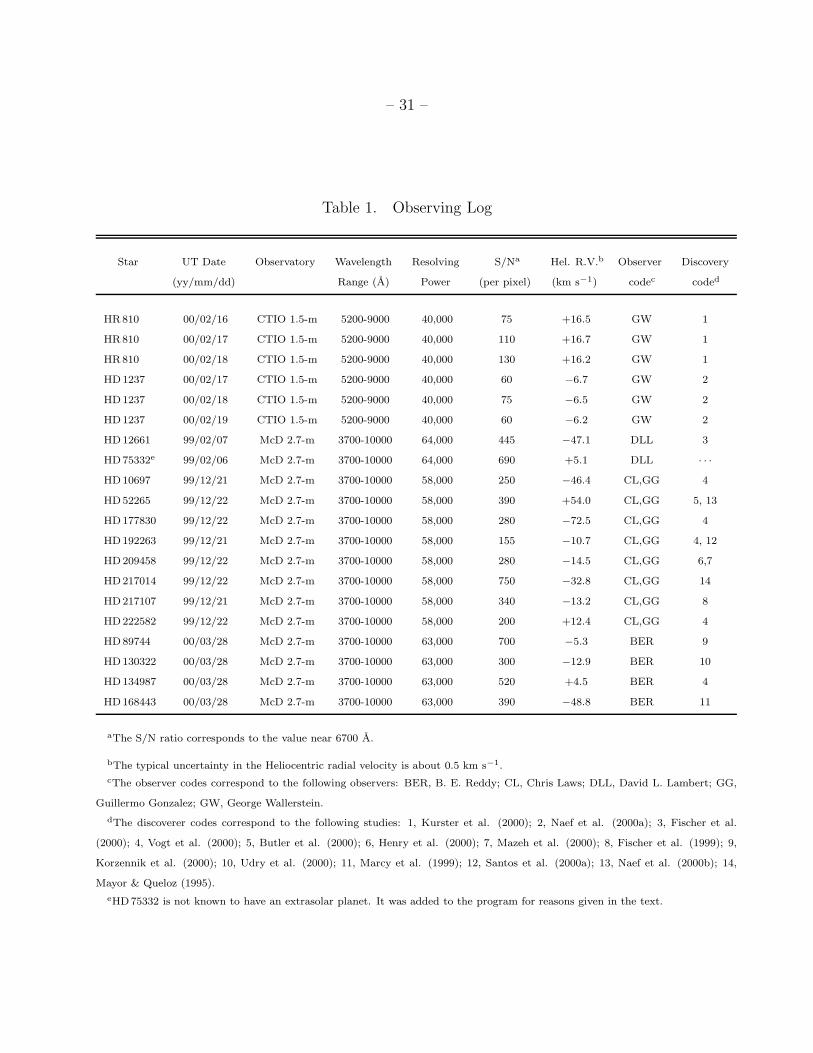
Table 1. Observing Log

Star UT Date Observatory Wavelength Resolving S/Na Hel. R.V.b Observer Discovery

(yy/mm/dd) Range (A) Power (per pixel) (km s−1) codec coded

HR810 00/02/16 CTIO 1.5-m 5200-9000 40,000 75 +16.5 GW 1

HR810 00/02/17 CTIO 1.5-m 5200-9000 40,000 110 +16.7 GW 1

HR810 00/02/18 CTIO 1.5-m 5200-9000 40,000 130 +16.2 GW 1

HD1237 00/02/17 CTIO 1.5-m 5200-9000 40,000 60 −6.7 GW 2

HD1237 00/02/18 CTIO 1.5-m 5200-9000 40,000 75 −6.5 GW 2

HD1237 00/02/19 CTIO 1.5-m 5200-9000 40,000 60 −6.2 GW 2

HD12661 99/02/07 McD 2.7-m 3700-10000 64,000 445 −47.1 DLL 3

HD75332e 99/02/06 McD 2.7-m 3700-10000 64,000 690 +5.1 DLL · · ·

HD10697 99/12/21 McD 2.7-m 3700-10000 58,000 250 −46.4 CL,GG 4

HD52265 99/12/22 McD 2.7-m 3700-10000 58,000 390 +54.0 CL,GG 5, 13

HD177830 99/12/22 McD 2.7-m 3700-10000 58,000 280 −72.5 CL,GG 4

HD192263 99/12/21 McD 2.7-m 3700-10000 58,000 155 −10.7 CL,GG 4, 12

HD209458 99/12/22 McD 2.7-m 3700-10000 58,000 280 −14.5 CL,GG 6,7

HD217014 99/12/22 McD 2.7-m 3700-10000 58,000 750 −32.8 CL,GG 14

HD217107 99/12/21 McD 2.7-m 3700-10000 58,000 340 −13.2 CL,GG 8

HD222582 99/12/22 McD 2.7-m 3700-10000 58,000 200 +12.4 CL,GG 4

HD89744 00/03/28 McD 2.7-m 3700-10000 63,000 700 −5.3 BER 9

HD130322 00/03/28 McD 2.7-m 3700-10000 63,000 300 −12.9 BER 10

HD134987 00/03/28 McD 2.7-m 3700-10000 63,000 520 +4.5 BER 4

HD168443 00/03/28 McD 2.7-m 3700-10000 63,000 390 −48.8 BER 11

aThe S/N ratio corresponds to the value near 6700 A.

bThe typical uncertainty in the Heliocentric radial velocity is about 0.5 km s−1.

cThe observer codes correspond to the following observers: BER, B. E. Reddy; CL, Chris Laws; DLL, David L. Lambert; GG,

Guillermo Gonzalez; GW, George Wallerstein.

dThe discoverer codes correspond to the following studies: 1, Kurster et al. (2000); 2, Naef et al. (2000a); 3, Fischer et al.

(2000); 4, Vogt et al. (2000); 5, Butler et al. (2000); 6, Henry et al. (2000); 7, Mazeh et al. (2000); 8, Fischer et al. (1999); 9,

Korzennik et al. (2000); 10, Udry et al. (2000); 11, Marcy et al. (1999); 12, Santos et al. (2000a); 13, Naef et al. (2000b); 14,

Mayor & Queloz (1995).

eHD75332 is not known to have an extrasolar planet. It was added to the program for reasons given in the text.

– 32 –

Table 2. Fe I and II lines Incorporated Since Paper V

Species λo χ1 log gf EW⊙

(A) (eV) (mA)

Fe I 6024.07 4.55 -0.12 118.0

Fe I 6093.65 4.61 -1.34 31.0

Fe I 6096.67 3.98 -1.81 37.2

Fe I 6098.25 4.56 -1.74 17.1

Fe I 6213.44 2.22 -2.66 83.5

Fe I 6820.37 4.64 -1.17 42.0

Fe I 7583.80 3.02 -1.90 85.7

Fe I 7586.03 4.31 -0.18 135.3

Fe II 5991.38 3.15 -3.48 30.3

Fe II 6442.95 5.55 -2.38 5.2

Fe II 6446.40 6.22 -1.92 4.0

– 33 –

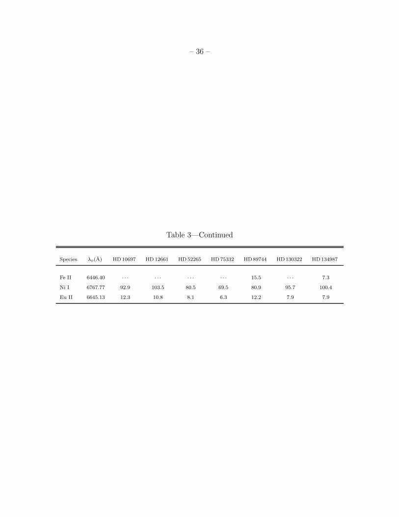
Table 3. Equivalent Widths for HD 10697, HD 12661, HD 52265, HD 89744, HD 130322,

and HD 134987

Species λo(A) HD 10697 HD 12661 HD 52265 HD 75332 HD89744 HD130322 HD134987

C I 5380.32 24.9 33.4 39.2 35.9 49.3 14.6 34.8

C I 6587.62 18.3 22.3 30.8 29.5 42.6 7.9 25.4

C I 7108.94 15.6 · · · · · · · · · · · · · · · · · ·

C I 7115.19 37.3 · · · 40.6 · · · 50.8 · · · · · ·

C I 7116.99 25.4 · · · 35.4 · · · 45.7 11.5 30.1

N I 7468.31 6.0 9.5 9.9 9.4 13.3 · · · 10.6

O I 7771.95 76.9 78.4 112.1 · · · 144.3 43.3 86.9

O I 7774.17 67.3 72.9 100.1 111.3 129.3 39.0 81.6

O I 7775.39 54.9 57.8 82.9 90.4 105.2 30.2 64.9

Na I 6154.23 49.7 73.0 43.9 32.5 40.1 55.2 68.9

Na I 6160.75 75.4 93.0 62.1 48.5 55.1 70.8 86.1

Mg I 5711.10 115.7 133.5 103.4 96.1 102.9 135.0 129.0

Al I 7835.32 54.9 90.5 52.6 39.5 50.0 58.4 67.6

Al I 7836.13 73.0 123.2 67.2 51.8 66.1 79.2 95.7

Si I 5793.08 55.4 · · · 54.6 · · · · · · 44.3 63.4

Si I 6125.03 42.5 54.6 43.7 37.0 42.3 31.7 52.2

Si I 6145.02 49.6 61.1 49.1 42.2 49.1 39.9 59.5

Si I 6721.84 55.8 77.5 57.2 47.6 57.2 49.8 65.1

S I 6046.11 27.3 30.0 30.2 24.5 33.6 17.4 32.1

S I 6052.68 17.8 22.9 22.0 23.0 · · · 9.0 23.7

S I 7686.13 6.5 · · · 4.6 · · · 11.9 · · · 8.3

Ca I 5867.57 32.1 40.2 23.4 21.1 24.3 37.7 38.1

Ca I 6166.44 81.0 91.1 69.5 65.4 70.4 91.6 87.9

Sc II 5526.79 93.3 95.9 92.6 86.1 108.4 73.2 95.2

Sc II 6604.60 51.7 54.9 47.7 38.0 56.1 38.6 53.3

Ti I 5965.83 39.0 50.3 28.2 24.5 25.0 49.1 51.3

Ti I 6126.22 33.9 41.3 19.7 13.7 15.0 44.8 37.4

Ti I 6261.10 65.9 75.7 43.6 35.8 40.5 77.6 69.8

Ti II 5336.77 86.4 87.3 87.9 · · · 101.3 69.5 85.9

Ti II 5418.75 64.8 63.8 62.7 · · · 74.7 48.6 60.7

Cr I 5787.97 56.6 65.9 49.3 · · · 44.2 · · · 62.2

Fe I 5044.21 · · · 91.3 71.6 · · · · · · 93.2 91.0

Fe I 5247.05 · · · 85.2 64.4 51.8 · · · 86.2 80.3

Fe I 5322.04 · · · · · · 60.1 52.8 · · · 76.3 77.7

Fe I 5651.47 · · · · · · · · · 17.1 · · · · · · · · ·

– 34 –

Table 3—Continued

Species λo(A) HD 10697 HD 12661 HD 52265 HD 75332 HD89744 HD130322 HD134987

Fe I 5652.32 · · · · · · · · · 23.4 · · · · · · · · ·

Fe I 5775.09 · · · · · · · · · 57.5 · · · · · · · · ·

Fe I 5806.73 64.3 77.1 59.2 54.0 59.3 67.5 75.0

Fe I 5814.80 · · · · · · · · · 19.4 · · · · · · · · ·

Fe I 5827.89 · · · · · · · · · 9.5 · · · · · · · · ·

Fe I 5852.19 54.0 60.5 44.9 38.0 41.4 53.1 58.0

Fe I 5853.18 15.7 16.9 · · · · · · · · · 19.1 19.8

Fe I 5855.13 34.4 39.5 25.4 20.2 22.9 31.3 38.0

Fe I 5856.08 44.3 51.5 36.6 30.8 34.8 44.0 49.0

Fe I 5956.70 68.3 · · · 43.9 33.3 38.4 70.1 65.5

Fe I 6024.07 · · · · · · 114.8 · · · · · · · · · · · ·

Fe I 6027.06 75.6 83.0 69.9 61.4 70.0 75.3 80.5

Fe I 6034.04 13.2 19.2 10.1 9.6 10.4 14.9 18.0

Fe I 6054.10 17.2 23.4 9.6 · · · · · · 16.8 21.0

Fe I 6055.99 · · · · · · · · · · · · · · · 88.3 91.0

Fe I 6079.02 · · · 69.0 · · · 45.0 · · · · · · · · ·

Fe I 6120.25 10.8 11.9 4.4 · · · · · · 11.8 11.0

Fe I 6151.62 63.8 69.6 47.6 36.8 42.9 66.1 66.0

Fe I 6157.73 · · · 80.1 67.2 61.1 67.9 74.5 86.6

Fe I 6159.41 20.2 25.3 13.4 12.7 14.3 19.5 22.5

Fe I 6165.37 57.1 64.2 49.8 40.8 44.7 55.2 61.9

Fe I 6180.22 · · · · · · · · · · · · · · · · · · 82.4

Fe I 6188.04 · · · 70.1 · · · · · · · · · 62.7 · · ·

Fe I 6226.77 42.3 48.8 31.6 25.6 30.2 41.1 43.7

Fe I 6229.23 52.6 63.5 43.0 31.7 39.4 54.4 61.5

Fe I 6240.66 65.2 69.5 47.0 37.5 45.9 64.9 67.9

Fe I 6265.13 · · · · · · · · · · · · · · · · · · 106.5

Fe I 6270.24 67.1 71.6 53.2 44.8 50.8 66.9 68.8

Fe I 6303.46 · · · 10.2 · · · · · · · · · · · · · · ·

Fe I 6380.75 65.1 74.9 57.3 50.3 56.0 64.1 68.8

Fe I 6385.74 17.5 22.6 12.9 · · · · · · 17.4 19.8

Fe I 6392.55 29.2 33.7 14.4 9.7 11.1 32.2 29.9

Fe I 6498.95 63.5 74.5 43.7 30.0 35.9 67.7 64.0

Fe I 6581.22 · · · 40.0 19.7 · · · 14.5 35.6 46.0

Fe I 6591.32 14.6 20.4 14.2 10.6 10.9 16.2 18.3

– 35 –

Table 3—Continued

Species λo(A) HD 10697 HD 12661 HD 52265 HD 75332 HD89744 HD130322 HD134987

Fe I 6608.03 30.8 35.3 14.3 12.9 12.8 32.9 33.8

Fe I 6627.56 38.6 48.6 32.2 24.4 30.3 39.2 49.2

Fe I 6646.98 20.9 23.6 10.0 · · · · · · 21.1 22.2

Fe I 6653.88 15.4 21.2 13.6 10.8 10.2 16.6 22.2

Fe I 6703.57 51.5 · · · 35.9 27.4 34.0 53.3 54.0

Fe I 6710.31 27.7 34.0 13.8 10.2 9.3 32.6 28.4

Fe I 6725.39 27.8 33.9 20.2 15.8 17.5 27.4 30.5

Fe I 6726.67 58.2 68.0 52.5 44.6 49.4 61.0 64.1

Fe I 6733.16 37.8 45.8 28.6 23.4 28.3 37.0 43.8

Fe I 6739.54 21.1 24.7 11.8 · · · 6.6 23.9 23.2

Fe I 6745.11 · · · 19.2 · · · · · · · · · 12.9 · · ·

Fe I 6745.96 · · · 16.6 7.8 · · · · · · 12.2 · · ·

Fe I 6746.96 · · · 10.1 3.9 · · · · · · 8.8 8.5

Fe I 6750.15 91.1 97.3 77.2 65.0 73.9 93.6 94.4

Fe I 6752.72 50.8 54.9 39.4 34.2 38.1 43.5 54.9

Fe I 6786.88 · · · 44.2 · · · · · · · · · · · · 41.6

Fe I 6820.43 · · · · · · 45.8 · · · · · · · · · · · ·

Fe I 6839.83 · · · · · · · · · · · · · · · · · · 46.5

Fe I 6855.74 · · · 38.1 23.2 · · · · · · 26.3 31.5

Fe I 6861.93 · · · 39.7 19.5 · · · · · · 34.1 34.2

Fe I 6862.48 43.0 51.2 32.8 · · · · · · 40.9 47.4

Fe I 6864.31 · · · 14.0 · · · · · · · · · 10.0 12.2

Fe I 7498.56 30.1 35.5 21.7 · · · 18.7 25.9 32.0

Fe I 7507.27 74.6 90.0 64.1 · · · 61.4 80.1 83.1

Fe I 7583.80 · · · · · · 85.5 · · · 83.7 · · · · · ·

Fe I 7586.03 · · · · · · 128.2 · · · 129.3 · · · · · ·

Fe II 5234.62 · · · 96.5 · · · · · · · · · 74.2 97.0

Fe II 5425.25 · · · · · · · · · 58.2 · · · · · · · · ·

Fe II 5991.37 · · · · · · 48.6 · · · 59.7 · · · 48.9

Fe II 6084.10 · · · 33.0 · · · 31.7 · · · 17.4 · · ·

Fe II 6149.25 47.3 47.1 56.6 54.3 68.0 29.3 48.3

Fe II 6247.55 65.4 63.7 74.5 · · · 90.3 42.1 65.4

Fe II 6369.46 28.5 29.6 35.0 27.3 42.5 15.6 30.3

Fe II 6416.92 · · · 54.1 · · · · · · · · · 38.6 · · ·

Fe II 6442.95 · · · · · · · · · · · · 14.8 · · · 8.3

– 36 –

Table 3—Continued

Species λo(A) HD 10697 HD 12661 HD 52265 HD 75332 HD89744 HD130322 HD134987

Fe II 6446.40 · · · · · · · · · · · · 15.5 · · · 7.3

Ni I 6767.77 92.9 103.5 80.5 69.5 80.9 95.7 100.4

Eu II 6645.13 12.3 10.8 8.1 6.3 12.2 7.9 7.9

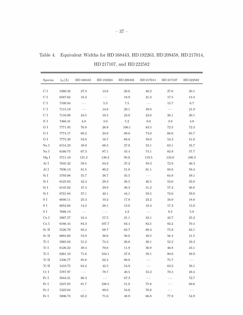
– 37 –

Table 4. Equivalent Widths for HD 168443, HD 192263, HD 209458, HD 217014,

HD 217107, and HD 222582

Species λo(A) HD168443 HD 192263 HD 209458 HD217014 HD 217107 HD222582

C I 5380.32 27.3 13.6 29.6 30.2 27.6 20.1

C I 6587.62 18.2 · · · 18.9 21.2 17.5 13.3

C I 7108.94 · · · 5.3 7.5 · · · 15.7 6.7

C I 7115.19 · · · 14.6 29.1 39.0 · · · 21.9

C I 7116.99 24.5 10.5 23.0 24.6 28.1 20.1

N I 7468.31 4.8 3.0 5.2 9.0 3.9 4.9

O I 7771.95 76.9 26.8 100.1 83.5 72.5 72.3

O I 7774.17 69.2 23.6 89.0 74.0 66.0 65.7

O I 7775.39 53.9 16.7 68.8 59.0 52.3 51.0

Na I 6154.23 49.9 68.5 27.0 52.1 63.1 35.7

Na I 6160.75 67.3 87.1 45.4 74.1 82.8 57.7

Mg I 5711.10 121.2 138.2 95.0 119.5 133.0 106.3

Al I 7835.32 59.5 64.9 37.2 59.3 72.9 46.3

Al I 7836.13 81.5 80.2 51.8 81.1 93.8 59.4

Si I 5793.08 55.7 38.7 45.5 · · · 64.8 49.1

Si I 6125.03 42.4 29.3 28.5 46.5 52.6 33.8

Si I 6145.02 47.4 29.9 38.3 51.2 57.2 40.8

Si I 6721.84 57.1 40.1 44.1 59.5 72.6 59.0

S I 6046.11 25.3 10.2 17.8 23.2 34.0 18.0

S I 6052.68 14.3 28.1 15.0 18.4 17.3 15.0

S I 7686.13 · · · · · · 4.3 · · · 9.2 5.8

Ca I 5867.57 34.4 57.5 31.1 33.1 42.7 25.3

Ca I 6166.44 83.3 107.7 63.4 82.5 92.2 70.4

Sc II 5526.79 93.4 68.7 82.7 89.4 75.9 82.1

Sc II 6604.60 53.9 36.6 38.6 49.5 56.4 41.5

Ti I 5965.83 51.2 74.2 20.6 38.1 52.2 33.3

Ti I 6126.22 39.4 70.6 11.9 30.9 46.8 23.1

Ti I 6261.10 71.6 104.1 37.9 59.1 80.6 49.9

Ti II 5336.77 85.6 62.2 80.0 · · · 75.7 · · ·

Ti II 5418.75 64.2 42.5 54.9 · · · 63.3 56.1

Cr I 5787.97 · · · 78.7 40.5 55.2 70.5 49.4

Fe I 5044.21 86.3 · · · 67.3 · · · · · · 72.7

Fe I 5247.05 81.7 108.5 51.0 75.8 · · · 69.6

Fe I 5322.04 · · · 89.0 54.6 70.8 · · · · · ·

Fe I 5806.73 65.2 71.6 48.9 66.8 77.8 54.9

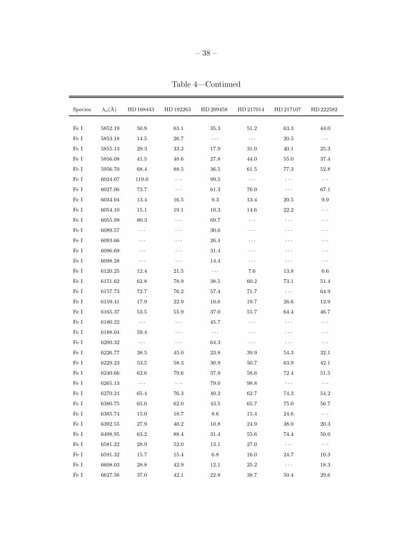
– 38 –

Table 4—Continued

Species λo(A) HD168443 HD 192263 HD 209458 HD217014 HD 217107 HD222582

Fe I 5852.19 50.9 63.1 35.3 51.2 63.3 44.0

Fe I 5853.18 14.5 26.7 · · · · · · 20.5 · · ·

Fe I 5855.13 29.3 33.2 17.9 31.0 40.1 25.3

Fe I 5856.08 41.5 48.6 27.8 44.0 55.0 37.4

Fe I 5956.70 68.4 88.5 36.5 61.5 77.3 52.8

Fe I 6024.07 119.0 · · · 99.5 · · · · · · · · ·

Fe I 6027.06 73.7 · · · 61.3 76.0 · · · 67.1

Fe I 6034.04 13.4 16.5 9.3 13.4 20.5 9.9

Fe I 6054.10 15.1 19.1 10.3 14.6 22.2 · · ·

Fe I 6055.99 80.3 · · · 69.7 · · · · · · · · ·

Fe I 6089.57 · · · · · · 30.6 · · · · · · · · ·

Fe I 6093.66 · · · · · · 26.4 · · · · · · · · ·

Fe I 6096.69 · · · · · · 31.4 · · · · · · · · ·

Fe I 6098.28 · · · · · · 14.4 · · · · · · · · ·

Fe I 6120.25 12.4 21.5 · · · 7.6 13.8 6.6

Fe I 6151.62 62.8 78.9 38.5 60.2 73.1 51.4

Fe I 6157.73 72.7 76.2 57.4 71.7 · · · 64.9

Fe I 6159.41 17.9 22.9 10.6 19.7 26.6 12.9

Fe I 6165.37 53.5 55.9 37.0 55.7 64.4 46.7

Fe I 6180.22 · · · · · · 45.7 · · · · · · · · ·

Fe I 6188.04 59.4 · · · · · · · · · · · · · · ·

Fe I 6200.32 · · · · · · 64.3 · · · · · · · · ·

Fe I 6226.77 38.5 45.0 23.8 39.9 54.3 32.1

Fe I 6229.23 53.5 58.3 30.9 50.7 63.9 42.1

Fe I 6240.66 62.6 79.6 37.9 58.6 72.4 51.5

Fe I 6265.13 · · · · · · 79.0 98.8 · · · · · ·

Fe I 6270.24 65.4 76.3 40.2 62.7 74.3 54.2

Fe I 6380.75 65.0 62.0 43.5 65.7 75.0 56.7

Fe I 6385.74 15.0 18.7 8.6 15.4 24.6 · · ·

Fe I 6392.55 27.9 40.2 10.8 24.9 38.0 20.3

Fe I 6498.95 63.2 88.4 31.4 55.6 74.4 50.0

Fe I 6581.22 28.9 52.0 13.1 27.0 · · · · · ·

Fe I 6591.32 15.7 15.4 6.8 16.0 24.7 10.3

Fe I 6608.03 28.8 42.9 12.1 25.2 · · · 18.3

Fe I 6627.56 37.0 42.1 22.8 38.7 50.4 29.6

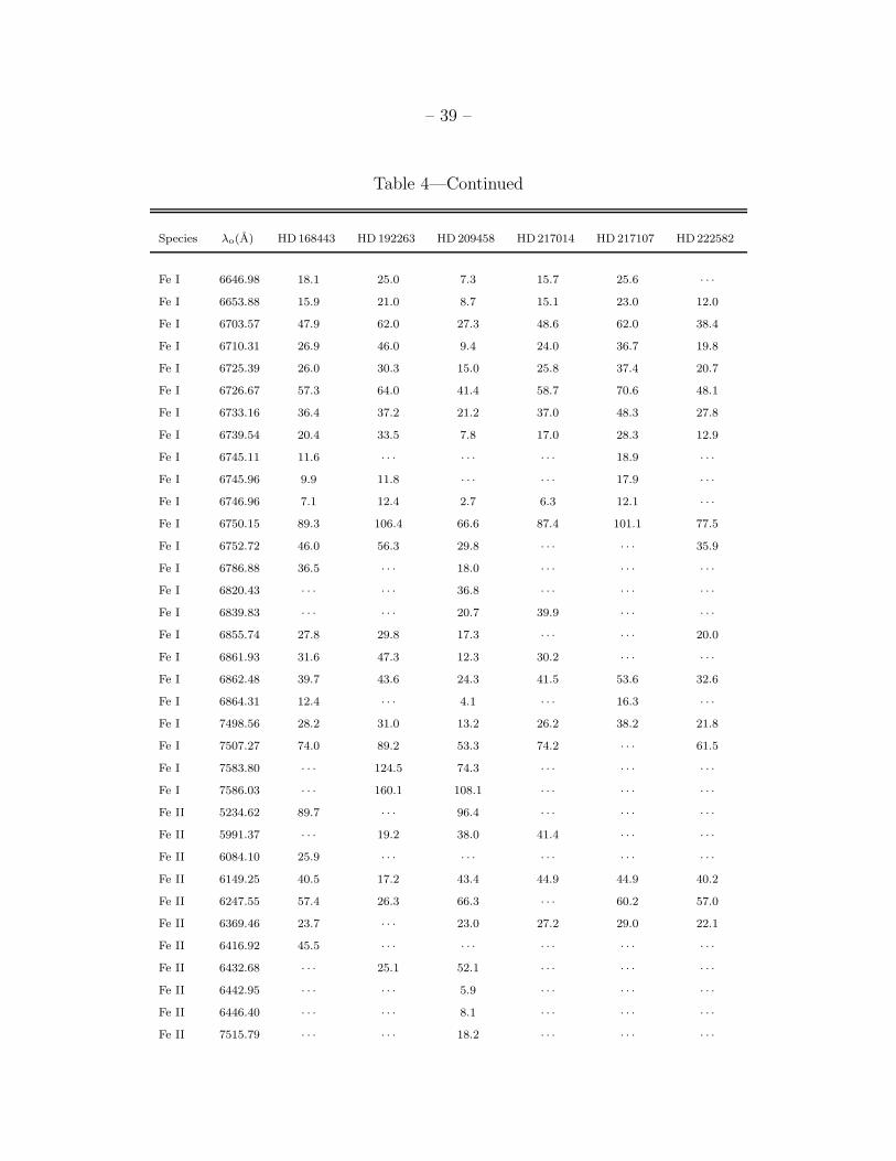
– 39 –

Table 4—Continued

Species λo(A) HD168443 HD 192263 HD 209458 HD217014 HD 217107 HD222582

Fe I 6646.98 18.1 25.0 7.3 15.7 25.6 · · ·

Fe I 6653.88 15.9 21.0 8.7 15.1 23.0 12.0

Fe I 6703.57 47.9 62.0 27.3 48.6 62.0 38.4

Fe I 6710.31 26.9 46.0 9.4 24.0 36.7 19.8

Fe I 6725.39 26.0 30.3 15.0 25.8 37.4 20.7

Fe I 6726.67 57.3 64.0 41.4 58.7 70.6 48.1

Fe I 6733.16 36.4 37.2 21.2 37.0 48.3 27.8

Fe I 6739.54 20.4 33.5 7.8 17.0 28.3 12.9

Fe I 6745.11 11.6 · · · · · · · · · 18.9 · · ·

Fe I 6745.96 9.9 11.8 · · · · · · 17.9 · · ·

Fe I 6746.96 7.1 12.4 2.7 6.3 12.1 · · ·

Fe I 6750.15 89.3 106.4 66.6 87.4 101.1 77.5

Fe I 6752.72 46.0 56.3 29.8 · · · · · · 35.9

Fe I 6786.88 36.5 · · · 18.0 · · · · · · · · ·

Fe I 6820.43 · · · · · · 36.8 · · · · · · · · ·

Fe I 6839.83 · · · · · · 20.7 39.9 · · · · · ·

Fe I 6855.74 27.8 29.8 17.3 · · · · · · 20.0

Fe I 6861.93 31.6 47.3 12.3 30.2 · · · · · ·

Fe I 6862.48 39.7 43.6 24.3 41.5 53.6 32.6

Fe I 6864.31 12.4 · · · 4.1 · · · 16.3 · · ·

Fe I 7498.56 28.2 31.0 13.2 26.2 38.2 21.8

Fe I 7507.27 74.0 89.2 53.3 74.2 · · · 61.5

Fe I 7583.80 · · · 124.5 74.3 · · · · · · · · ·

Fe I 7586.03 · · · 160.1 108.1 · · · · · · · · ·

Fe II 5234.62 89.7 · · · 96.4 · · · · · · · · ·

Fe II 5991.37 · · · 19.2 38.0 41.4 · · · · · ·

Fe II 6084.10 25.9 · · · · · · · · · · · · · · ·

Fe II 6149.25 40.5 17.2 43.4 44.9 44.9 40.2

Fe II 6247.55 57.4 26.3 66.3 · · · 60.2 57.0

Fe II 6369.46 23.7 · · · 23.0 27.2 29.0 22.1

Fe II 6416.92 45.5 · · · · · · · · · · · · · · ·

Fe II 6432.68 · · · 25.1 52.1 · · · · · · · · ·

Fe II 6442.95 · · · · · · 5.9 · · · · · · · · ·

Fe II 6446.40 · · · · · · 8.1 · · · · · · · · ·

Fe II 7515.79 · · · · · · 18.2 · · · · · · · · ·

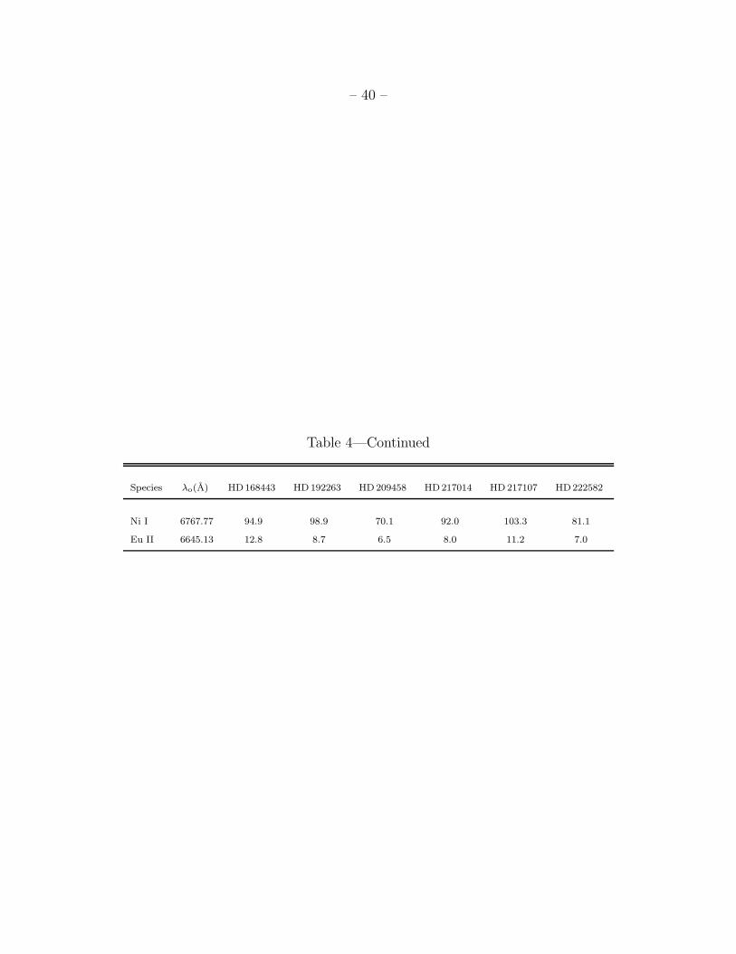
– 40 –

Table 4—Continued

Species λo(A) HD168443 HD 192263 HD 209458 HD217014 HD 217107 HD222582

Ni I 6767.77 94.9 98.9 70.1 92.0 103.3 81.1

Eu II 6645.13 12.8 8.7 6.5 8.0 11.2 7.0

– 41 –

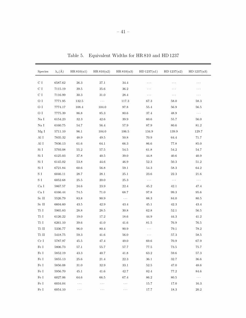
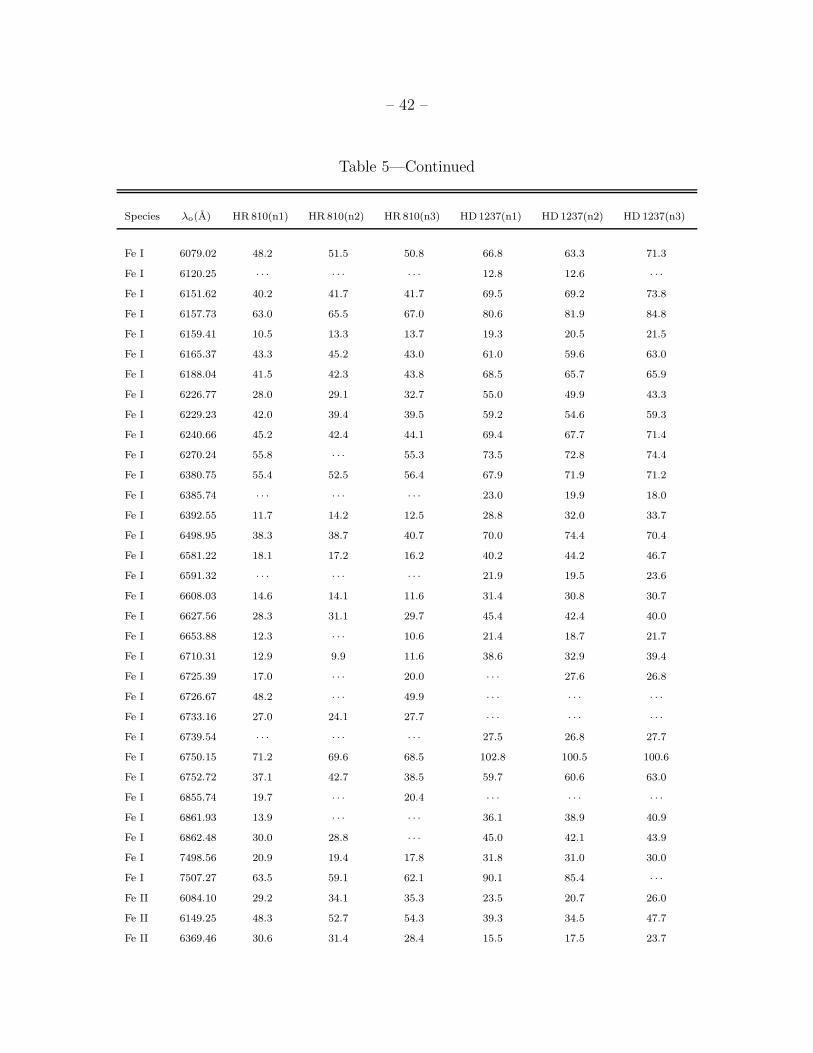
Table 5. Equivalent Widths for HR810 and HD 1237

Species λo(A) HR 810(n1) HR 810(n2) HR 810(n3) HD1237(n1) HD 1237(n2) HD 1237(n3)

C I 6587.62 26.3 27.1 34.4 · · · · · · · · ·

C I 7115.19 39.5 35.6 36.2 · · · · · · · · ·

C I 7116.99 30.3 31.0 28.4 · · · · · · · · ·

O I 7771.95 132.5 · · · 117.3 67.3 58.0 58.3

O I 7774.17 108.4 104.0 97.8 55.4 56.9 56.5

O I 7775.39 86.8 85.3 80.6 37.4 48.9 · · ·

Na I 6154.23 32.3 42.6 39.9 60.6 55.7 56.0

Na I 6160.75 54.7 56.4 57.9 87.9 80.6 81.2

Mg I 5711.10 96.1 104.0 106.5 134.9 139.9 129.7

Al I 7835.32 48.9 49.5 50.8 70.9 64.4 71.7

Al I 7836.13 61.6 64.1 66.3 86.6 77.8 85.0

Si I 5793.08 55.2 57.5 54.5 61.8 54.2 54.7

Si I 6125.03 37.8 40.5 39.0 44.8 40.6 40.9

Si I 6145.02 53.8 44.6 46.9 52.3 50.3 51.2

Si I 6721.84 60.6 56.8 59.1 54.3 58.3 64.2

S I 6046.11 28.7 28.1 25.1 23.6 22.3 21.6

S I 6052.68 25.5 20.0 25.3 · · · · · · · · ·

Ca I 5867.57 24.6 23.9 22.4 45.2 42.1 47.4

Ca I 6166.44 74.5 71.0 68.7 97.8 99.3 95.6

Sc II 5526.79 83.8 90.9 · · · 88.3 84.0 80.5

Sc II 6604.60 43.5 42.9 43.4 45.1 42.3 43.4

Ti I 5965.83 28.8 28.5 30.8 62.8 52.1 56.5

Ti I 6126.22 19.0 17.2 18.6 44.9 44.3 41.2

Ti I 6261.10 39.6 41.0 41.6 81.5 76.9 76.5

Ti II 5336.77 96.0 80.4 90.9 · · · 79.1 78.2

Ti II 5418.75 59.3 41.6 56.0 · · · 57.3 58.5

Cr I 5787.97 45.5 47.4 49.0 69.6 70.9 67.9

Fe I 5806.73 57.1 55.7 57.7 77.5 73.5 75.7

Fe I 5852.19 43.3 40.7 41.8 63.2 59.6 57.3

Fe I 5855.13 25.6 21.4 22.3 36.1 32.7 36.6

Fe I 5856.08 31.0 32.9 33.1 52.5 47.0 48.6

Fe I 5956.70 45.1 41.6 42.7 82.4 77.2 84.6

Fe I 6027.06 64.6 66.5 67.4 86.2 80.5 · · ·

Fe I 6034.04 · · · · · · · · · 15.7 17.0 16.3

Fe I 6054.10 · · · · · · · · · 17.7 18.3 20.2

– 42 –

Table 5—Continued

Species λo(A) HR 810(n1) HR 810(n2) HR 810(n3) HD1237(n1) HD 1237(n2) HD 1237(n3)

Fe I 6079.02 48.2 51.5 50.8 66.8 63.3 71.3

Fe I 6120.25 · · · · · · · · · 12.8 12.6 · · ·

Fe I 6151.62 40.2 41.7 41.7 69.5 69.2 73.8

Fe I 6157.73 63.0 65.5 67.0 80.6 81.9 84.8

Fe I 6159.41 10.5 13.3 13.7 19.3 20.5 21.5

Fe I 6165.37 43.3 45.2 43.0 61.0 59.6 63.0

Fe I 6188.04 41.5 42.3 43.8 68.5 65.7 65.9

Fe I 6226.77 28.0 29.1 32.7 55.0 49.9 43.3

Fe I 6229.23 42.0 39.4 39.5 59.2 54.6 59.3

Fe I 6240.66 45.2 42.4 44.1 69.4 67.7 71.4

Fe I 6270.24 55.8 · · · 55.3 73.5 72.8 74.4

Fe I 6380.75 55.4 52.5 56.4 67.9 71.9 71.2

Fe I 6385.74 · · · · · · · · · 23.0 19.9 18.0

Fe I 6392.55 11.7 14.2 12.5 28.8 32.0 33.7

Fe I 6498.95 38.3 38.7 40.7 70.0 74.4 70.4

Fe I 6581.22 18.1 17.2 16.2 40.2 44.2 46.7

Fe I 6591.32 · · · · · · · · · 21.9 19.5 23.6

Fe I 6608.03 14.6 14.1 11.6 31.4 30.8 30.7

Fe I 6627.56 28.3 31.1 29.7 45.4 42.4 40.0

Fe I 6653.88 12.3 · · · 10.6 21.4 18.7 21.7

Fe I 6710.31 12.9 9.9 11.6 38.6 32.9 39.4

Fe I 6725.39 17.0 · · · 20.0 · · · 27.6 26.8

Fe I 6726.67 48.2 · · · 49.9 · · · · · · · · ·

Fe I 6733.16 27.0 24.1 27.7 · · · · · · · · ·

Fe I 6739.54 · · · · · · · · · 27.5 26.8 27.7

Fe I 6750.15 71.2 69.6 68.5 102.8 100.5 100.6

Fe I 6752.72 37.1 42.7 38.5 59.7 60.6 63.0

Fe I 6855.74 19.7 · · · 20.4 · · · · · · · · ·

Fe I 6861.93 13.9 · · · · · · 36.1 38.9 40.9

Fe I 6862.48 30.0 28.8 · · · 45.0 42.1 43.9

Fe I 7498.56 20.9 19.4 17.8 31.8 31.0 30.0

Fe I 7507.27 63.5 59.1 62.1 90.1 85.4 · · ·

Fe II 6084.10 29.2 34.1 35.3 23.5 20.7 26.0

Fe II 6149.25 48.3 52.7 54.3 39.3 34.5 47.7

Fe II 6369.46 30.6 31.4 28.4 15.5 17.5 23.7

– 43 –

Table 5—Continued

Species λo(A) HR 810(n1) HR 810(n2) HR 810(n3) HD1237(n1) HD 1237(n2) HD 1237(n3)

Fe II 6416.92 53.2 50.8 52.1 49.5 43.4 46.2

Ni I 6767.77 79.6 75.1 75.4 110.7 103.6 98.0

Eu II 6645.13 8.9 · · · 11.8 · · · · · · · · ·

– 44 –

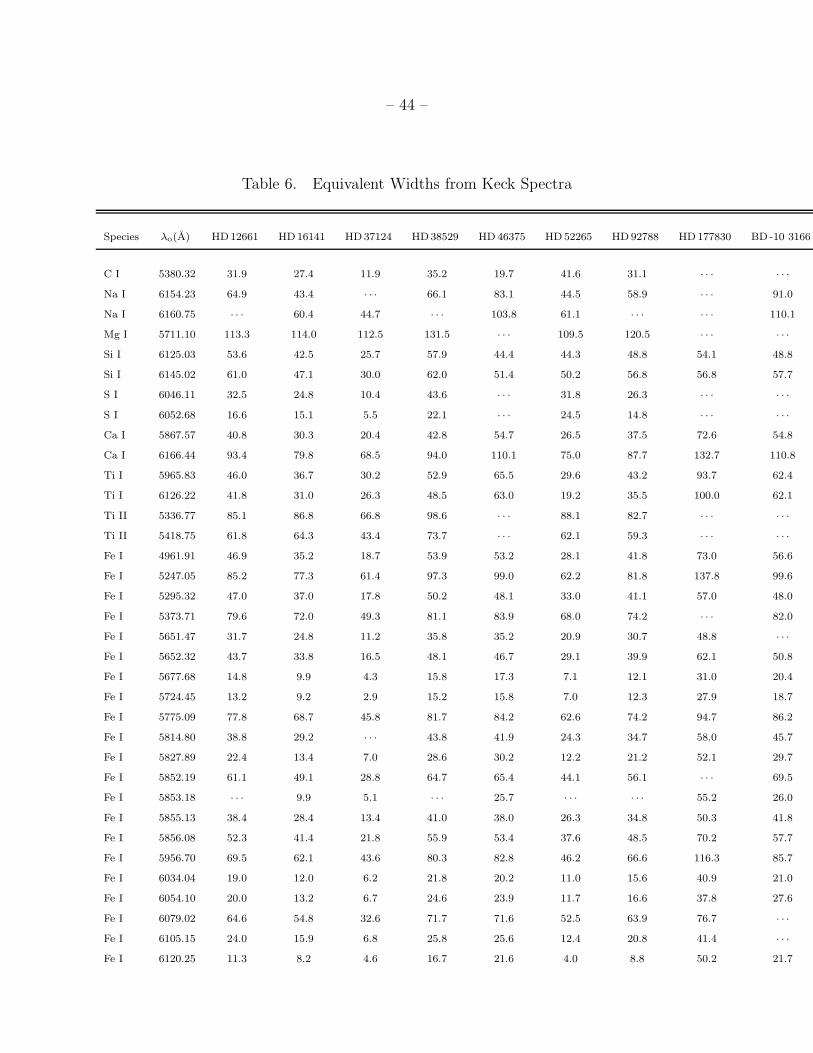
Table 6. Equivalent Widths from Keck Spectra

Species λo(A) HD12661 HD16141 HD37124 HD38529 HD 46375 HD 52265 HD 92788 HD 177830 BD -10 3166

C I 5380.32 31.9 27.4 11.9 35.2 19.7 41.6 31.1 · · · · · ·

Na I 6154.23 64.9 43.4 · · · 66.1 83.1 44.5 58.9 · · · 91.0

Na I 6160.75 · · · 60.4 44.7 · · · 103.8 61.1 · · · · · · 110.1

Mg I 5711.10 113.3 114.0 112.5 131.5 · · · 109.5 120.5 · · · · · ·

Si I 6125.03 53.6 42.5 25.7 57.9 44.4 44.3 48.8 54.1 48.8

Si I 6145.02 61.0 47.1 30.0 62.0 51.4 50.2 56.8 56.8 57.7

S I 6046.11 32.5 24.8 10.4 43.6 · · · 31.8 26.3 · · · · · ·

S I 6052.68 16.6 15.1 5.5 22.1 · · · 24.5 14.8 · · · · · ·

Ca I 5867.57 40.8 30.3 20.4 42.8 54.7 26.5 37.5 72.6 54.8

Ca I 6166.44 93.4 79.8 68.5 94.0 110.1 75.0 87.7 132.7 110.8

Ti I 5965.83 46.0 36.7 30.2 52.9 65.5 29.6 43.2 93.7 62.4

Ti I 6126.22 41.8 31.0 26.3 48.5 63.0 19.2 35.5 100.0 62.1

Ti II 5336.77 85.1 86.8 66.8 98.6 · · · 88.1 82.7 · · · · · ·

Ti II 5418.75 61.8 64.3 43.4 73.7 · · · 62.1 59.3 · · · · · ·

Fe I 4961.91 46.9 35.2 18.7 53.9 53.2 28.1 41.8 73.0 56.6

Fe I 5247.05 85.2 77.3 61.4 97.3 99.0 62.2 81.8 137.8 99.6

Fe I 5295.32 47.0 37.0 17.8 50.2 48.1 33.0 41.1 57.0 48.0

Fe I 5373.71 79.6 72.0 49.3 81.1 83.9 68.0 74.2 · · · 82.0

Fe I 5651.47 31.7 24.8 11.2 35.8 35.2 20.9 30.7 48.8 · · ·

Fe I 5652.32 43.7 33.8 16.5 48.1 46.7 29.1 39.9 62.1 50.8

Fe I 5677.68 14.8 9.9 4.3 15.8 17.3 7.1 12.1 31.0 20.4

Fe I 5724.45 13.2 9.2 2.9 15.2 15.8 7.0 12.3 27.9 18.7

Fe I 5775.09 77.8 68.7 45.8 81.7 84.2 62.6 74.2 94.7 86.2

Fe I 5814.80 38.8 29.2 · · · 43.8 41.9 24.3 34.7 58.0 45.7

Fe I 5827.89 22.4 13.4 7.0 28.6 30.2 12.2 21.2 52.1 29.7

Fe I 5852.19 61.1 49.1 28.8 64.7 65.4 44.1 56.1 · · · 69.5

Fe I 5853.18 · · · 9.9 5.1 · · · 25.7 · · · · · · 55.2 26.0

Fe I 5855.13 38.4 28.4 13.4 41.0 38.0 26.3 34.8 50.3 41.8

Fe I 5856.08 52.3 41.4 21.8 55.9 53.4 37.6 48.5 70.2 57.7

Fe I 5956.70 69.5 62.1 43.6 80.3 82.8 46.2 66.6 116.3 85.7

Fe I 6034.04 19.0 12.0 6.2 21.8 20.2 11.0 15.6 40.9 21.0

Fe I 6054.10 20.0 13.2 6.7 24.6 23.9 11.7 16.6 37.8 27.6

Fe I 6079.02 64.6 54.8 32.6 71.7 71.6 52.5 63.9 76.7 · · ·

Fe I 6105.15 24.0 15.9 6.8 25.8 25.6 12.4 20.8 41.4 · · ·

Fe I 6120.25 11.3 8.2 4.6 16.7 21.6 4.0 8.8 50.2 21.7

– 45 –

Table 6—Continued

Species λo(A) HD12661 HD16141 HD37124 HD38529 HD 46375 HD 52265 HD 92788 HD 177830 BD -10 3166

Fe I 6151.62 69.0 59.2 41.5 78.1 77.1 49.3 65.1 104.1 79.2

Fe I 6157.73 79.7 72.4 50.0 88.8 81.9 67.0 76.1 105.0 81.4

Fe I 6159.41 26.3 17.4 6.8 28.7 29.8 14.6 22.5 48.8 34.1

Fe I 6165.37 64.7 55.3 32.6 69.4 66.9 48.9 60.5 76.3 69.3

Fe II 5325.56 51.0 54.6 25.3 · · · 33.9 61.7 50.8 · · · · · ·

Fe II 5414.05 38.7 38.2 14.6 52.3 24.3 44.2 37.4 34.5 27.2

Fe II 5425.25 53.0 53.5 25.1 64.9 39.3 57.8 51.4 49.5 · · ·

Fe II 6149.25 47.1 47.9 20.9 57.3 30.0 58.6 46.9 41.3 33.6

Cr I 5787.97 65.3 53.2 33.5 70.3 76.9 · · · 63.3 · · · 85.0

– 46 –

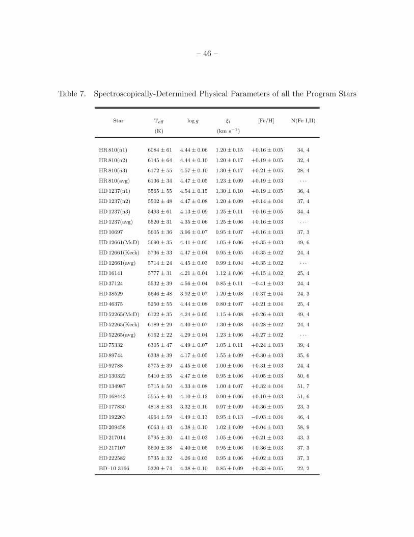
Table 7. Spectroscopically-Determined Physical Parameters of all the Program Stars

Star Teff log g ξt [Fe/H] N(Fe I,II)

(K) (km s−1)

HR 810(n1) 6084 ± 61 4.44 ± 0.06 1.20 ± 0.15 +0.16 ± 0.05 34, 4

HR 810(n2) 6145 ± 64 4.44 ± 0.10 1.20 ± 0.17 +0.19 ± 0.05 32, 4

HR 810(n3) 6172 ± 55 4.57 ± 0.10 1.30 ± 0.17 +0.21 ± 0.05 28, 4

HR 810(avg) 6136 ± 34 4.47 ± 0.05 1.23 ± 0.09 +0.19 ± 0.03 · · ·

HD 1237(n1) 5565 ± 55 4.54 ± 0.15 1.30 ± 0.10 +0.19 ± 0.05 36, 4

HD 1237(n2) 5502 ± 48 4.47 ± 0.08 1.20 ± 0.09 +0.14 ± 0.04 37, 4

HD 1237(n3) 5493 ± 61 4.13 ± 0.09 1.25 ± 0.11 +0.16 ± 0.05 34, 4

HD 1237(avg) 5520 ± 31 4.35 ± 0.06 1.25 ± 0.06 +0.16 ± 0.03 · · ·

HD 10697 5605 ± 36 3.96 ± 0.07 0.95 ± 0.07 +0.16 ± 0.03 37, 3

HD 12661(McD) 5690 ± 35 4.41 ± 0.05 1.05 ± 0.06 +0.35 ± 0.03 49, 6

HD 12661(Keck) 5736 ± 33 4.47 ± 0.04 0.95 ± 0.05 +0.35 ± 0.02 24, 4

HD 12661(avg) 5714 ± 24 4.45 ± 0.03 0.99 ± 0.04 +0.35 ± 0.02 · · ·

HD 16141 5777 ± 31 4.21 ± 0.04 1.12 ± 0.06 +0.15 ± 0.02 25, 4

HD 37124 5532 ± 39 4.56 ± 0.04 0.85 ± 0.11 −0.41 ± 0.03 24, 4

HD 38529 5646 ± 48 3.92 ± 0.07 1.20 ± 0.08 +0.37 ± 0.04 24, 3

HD 46375 5250 ± 55 4.44 ± 0.08 0.80 ± 0.07 +0.21 ± 0.04 25, 4

HD 52265(McD) 6122 ± 35 4.24 ± 0.05 1.15 ± 0.08 +0.26 ± 0.03 49, 4

HD 52265(Keck) 6189 ± 29 4.40 ± 0.07 1.30 ± 0.08 +0.28 ± 0.02 24, 4

HD 52265(avg) 6162 ± 22 4.29 ± 0.04 1.23 ± 0.06 +0.27 ± 0.02 · · ·

HD 75332 6305 ± 47 4.49 ± 0.07 1.05 ± 0.11 +0.24 ± 0.03 39, 4

HD 89744 6338 ± 39 4.17 ± 0.05 1.55 ± 0.09 +0.30 ± 0.03 35, 6

HD 92788 5775 ± 39 4.45 ± 0.05 1.00 ± 0.06 +0.31 ± 0.03 24, 4

HD 130322 5410 ± 35 4.47 ± 0.08 0.95 ± 0.06 +0.05 ± 0.03 50, 6

HD 134987 5715 ± 50 4.33 ± 0.08 1.00 ± 0.07 +0.32 ± 0.04 51, 7

HD 168443 5555 ± 40 4.10 ± 0.12 0.90 ± 0.06 +0.10 ± 0.03 51, 6

HD 177830 4818 ± 83 3.32 ± 0.16 0.97 ± 0.09 +0.36 ± 0.05 23, 3

HD 192263 4964 ± 59 4.49 ± 0.13 0.95 ± 0.13 −0.03 ± 0.04 46, 4

HD 209458 6063 ± 43 4.38 ± 0.10 1.02 ± 0.09 +0.04 ± 0.03 58, 9

HD 217014 5795 ± 30 4.41 ± 0.03 1.05 ± 0.06 +0.21 ± 0.03 43, 3

HD 217107 5600 ± 38 4.40 ± 0.05 0.95 ± 0.06 +0.36 ± 0.03 37, 3

HD 222582 5735 ± 32 4.26 ± 0.03 0.95 ± 0.06 +0.02 ± 0.03 37, 3

BD -10 3166 5320 ± 74 4.38 ± 0.10 0.85 ± 0.09 +0.33 ± 0.05 22, 2

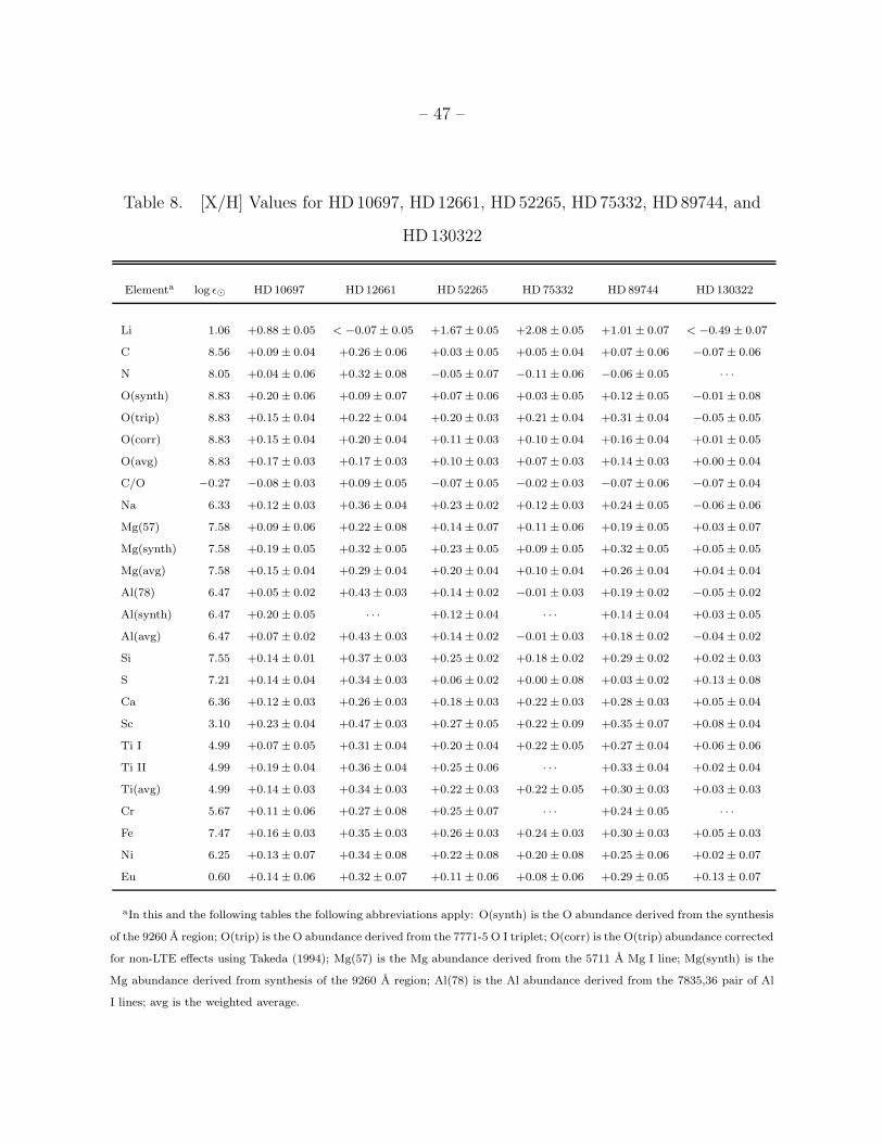
– 47 –

Table 8. [X/H] Values for HD 10697, HD 12661, HD 52265, HD 75332, HD 89744, and

HD 130322

Elementa log ǫ⊙ HD10697 HD12661 HD52265 HD 75332 HD 89744 HD 130322

Li 1.06 +0.88 ± 0.05 < −0.07 ± 0.05 +1.67 ± 0.05 +2.08 ± 0.05 +1.01 ± 0.07 < −0.49 ± 0.07

C 8.56 +0.09 ± 0.04 +0.26 ± 0.06 +0.03 ± 0.05 +0.05 ± 0.04 +0.07 ± 0.06 −0.07 ± 0.06

N 8.05 +0.04 ± 0.06 +0.32 ± 0.08 −0.05 ± 0.07 −0.11 ± 0.06 −0.06 ± 0.05 · · ·

O(synth) 8.83 +0.20 ± 0.06 +0.09 ± 0.07 +0.07 ± 0.06 +0.03 ± 0.05 +0.12 ± 0.05 −0.01 ± 0.08

O(trip) 8.83 +0.15 ± 0.04 +0.22 ± 0.04 +0.20 ± 0.03 +0.21 ± 0.04 +0.31 ± 0.04 −0.05 ± 0.05

O(corr) 8.83 +0.15 ± 0.04 +0.20 ± 0.04 +0.11 ± 0.03 +0.10 ± 0.04 +0.16 ± 0.04 +0.01 ± 0.05

O(avg) 8.83 +0.17 ± 0.03 +0.17 ± 0.03 +0.10 ± 0.03 +0.07 ± 0.03 +0.14 ± 0.03 +0.00 ± 0.04

C/O −0.27 −0.08 ± 0.03 +0.09 ± 0.05 −0.07 ± 0.05 −0.02 ± 0.03 −0.07 ± 0.06 −0.07 ± 0.04

Na 6.33 +0.12 ± 0.03 +0.36 ± 0.04 +0.23 ± 0.02 +0.12 ± 0.03 +0.24 ± 0.05 −0.06 ± 0.06

Mg(57) 7.58 +0.09 ± 0.06 +0.22 ± 0.08 +0.14 ± 0.07 +0.11 ± 0.06 +0.19 ± 0.05 +0.03 ± 0.07

Mg(synth) 7.58 +0.19 ± 0.05 +0.32 ± 0.05 +0.23 ± 0.05 +0.09 ± 0.05 +0.32 ± 0.05 +0.05 ± 0.05

Mg(avg) 7.58 +0.15 ± 0.04 +0.29 ± 0.04 +0.20 ± 0.04 +0.10 ± 0.04 +0.26 ± 0.04 +0.04 ± 0.04

Al(78) 6.47 +0.05 ± 0.02 +0.43 ± 0.03 +0.14 ± 0.02 −0.01 ± 0.03 +0.19 ± 0.02 −0.05 ± 0.02

Al(synth) 6.47 +0.20 ± 0.05 · · · +0.12 ± 0.04 · · · +0.14 ± 0.04 +0.03 ± 0.05

Al(avg) 6.47 +0.07 ± 0.02 +0.43 ± 0.03 +0.14 ± 0.02 −0.01 ± 0.03 +0.18 ± 0.02 −0.04 ± 0.02

Si 7.55 +0.14 ± 0.01 +0.37 ± 0.03 +0.25 ± 0.02 +0.18 ± 0.02 +0.29 ± 0.02 +0.02 ± 0.03

S 7.21 +0.14 ± 0.04 +0.34 ± 0.03 +0.06 ± 0.02 +0.00 ± 0.08 +0.03 ± 0.02 +0.13 ± 0.08

Ca 6.36 +0.12 ± 0.03 +0.26 ± 0.03 +0.18 ± 0.03 +0.22 ± 0.03 +0.28 ± 0.03 +0.05 ± 0.04

Sc 3.10 +0.23 ± 0.04 +0.47 ± 0.03 +0.27 ± 0.05 +0.22 ± 0.09 +0.35 ± 0.07 +0.08 ± 0.04

Ti I 4.99 +0.07 ± 0.05 +0.31 ± 0.04 +0.20 ± 0.04 +0.22 ± 0.05 +0.27 ± 0.04 +0.06 ± 0.06

Ti II 4.99 +0.19 ± 0.04 +0.36 ± 0.04 +0.25 ± 0.06 · · · +0.33 ± 0.04 +0.02 ± 0.04

Ti(avg) 4.99 +0.14 ± 0.03 +0.34 ± 0.03 +0.22 ± 0.03 +0.22 ± 0.05 +0.30 ± 0.03 +0.03 ± 0.03

Cr 5.67 +0.11 ± 0.06 +0.27 ± 0.08 +0.25 ± 0.07 · · · +0.24 ± 0.05 · · ·

Fe 7.47 +0.16 ± 0.03 +0.35 ± 0.03 +0.26 ± 0.03 +0.24 ± 0.03 +0.30 ± 0.03 +0.05 ± 0.03

Ni 6.25 +0.13 ± 0.07 +0.34 ± 0.08 +0.22 ± 0.08 +0.20 ± 0.08 +0.25 ± 0.06 +0.02 ± 0.07

Eu 0.60 +0.14 ± 0.06 +0.32 ± 0.07 +0.11 ± 0.06 +0.08 ± 0.06 +0.29 ± 0.05 +0.13 ± 0.07

aIn this and the following tables the following abbreviations apply: O(synth) is the O abundance derived from the synthesis

of the 9260 A region; O(trip) is the O abundance derived from the 7771-5 O I triplet; O(corr) is the O(trip) abundance corrected

for non-LTE effects using Takeda (1994); Mg(57) is the Mg abundance derived from the 5711 A Mg I line; Mg(synth) is the

Mg abundance derived from synthesis of the 9260 A region; Al(78) is the Al abundance derived from the 7835,36 pair of Al

I lines; avg is the weighted average.

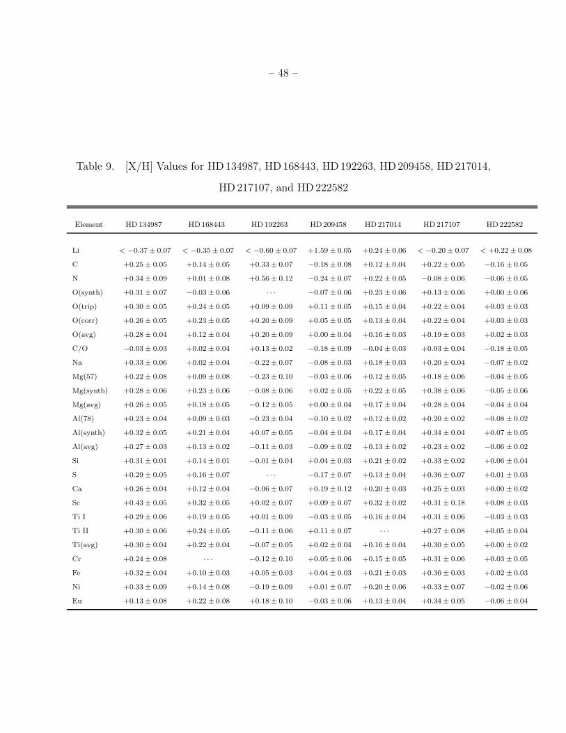
– 48 –

Table 9. [X/H] Values for HD 134987, HD 168443, HD 192263, HD 209458, HD 217014,

HD 217107, and HD 222582

Element HD134987 HD168443 HD192263 HD209458 HD217014 HD 217107 HD222582

Li < −0.37 ± 0.07 < −0.35 ± 0.07 < −0.60 ± 0.07 +1.59 ± 0.05 +0.24 ± 0.06 < −0.20 ± 0.07 < +0.22 ± 0.08

C +0.25 ± 0.05 +0.14 ± 0.05 +0.33 ± 0.07 −0.18 ± 0.08 +0.12 ± 0.04 +0.22 ± 0.05 −0.16 ± 0.05

N +0.34 ± 0.09 +0.01 ± 0.08 +0.56 ± 0.12 −0.24 ± 0.07 +0.22 ± 0.05 −0.08 ± 0.06 −0.06 ± 0.05

O(synth) +0.31 ± 0.07 −0.03 ± 0.06 · · · −0.07 ± 0.06 +0.23 ± 0.06 +0.13 ± 0.06 +0.00 ± 0.06

O(trip) +0.30 ± 0.05 +0.24 ± 0.05 +0.09 ± 0.09 +0.11 ± 0.05 +0.15 ± 0.04 +0.22 ± 0.04 +0.03 ± 0.03

O(corr) +0.26 ± 0.05 +0.23 ± 0.05 +0.20 ± 0.09 +0.05 ± 0.05 +0.13 ± 0.04 +0.22 ± 0.04 +0.03 ± 0.03

O(avg) +0.28 ± 0.04 +0.12 ± 0.04 +0.20 ± 0.09 +0.00 ± 0.04 +0.16 ± 0.03 +0.19 ± 0.03 +0.02 ± 0.03

C/O −0.03 ± 0.03 +0.02 ± 0.04 +0.13 ± 0.02 −0.18 ± 0.09 −0.04 ± 0.03 +0.03 ± 0.04 −0.18 ± 0.05

Na +0.33 ± 0.06 +0.02 ± 0.04 −0.22 ± 0.07 −0.08 ± 0.03 +0.18 ± 0.03 +0.20 ± 0.04 −0.07 ± 0.02

Mg(57) +0.22 ± 0.08 +0.09 ± 0.08 −0.23 ± 0.10 −0.03 ± 0.06 +0.12 ± 0.05 +0.18 ± 0.06 −0.04 ± 0.05

Mg(synth) +0.28 ± 0.06 +0.23 ± 0.06 −0.08 ± 0.06 +0.02 ± 0.05 +0.22 ± 0.05 +0.38 ± 0.06 −0.05 ± 0.06

Mg(avg) +0.26 ± 0.05 +0.18 ± 0.05 −0.12 ± 0.05 +0.00 ± 0.04 +0.17 ± 0.04 +0.28 ± 0.04 −0.04 ± 0.04

Al(78) +0.23 ± 0.04 +0.09 ± 0.03 −0.23 ± 0.04 −0.10 ± 0.02 +0.12 ± 0.02 +0.20 ± 0.02 −0.08 ± 0.02

Al(synth) +0.32 ± 0.05 +0.21 ± 0.04 +0.07 ± 0.05 −0.04 ± 0.04 +0.17 ± 0.04 +0.34 ± 0.04 +0.07 ± 0.05

Al(avg) +0.27 ± 0.03 +0.13 ± 0.02 −0.11 ± 0.03 −0.09 ± 0.02 +0.13 ± 0.02 +0.23 ± 0.02 −0.06 ± 0.02

Si +0.31 ± 0.01 +0.14 ± 0.01 −0.01 ± 0.04 +0.04 ± 0.03 +0.21 ± 0.02 +0.33 ± 0.02 +0.06 ± 0.04

S +0.29 ± 0.05 +0.16 ± 0.07 · · · −0.17 ± 0.07 +0.13 ± 0.04 +0.36 ± 0.07 +0.01 ± 0.03

Ca +0.26 ± 0.04 +0.12 ± 0.04 −0.06 ± 0.07 +0.19 ± 0.12 +0.20 ± 0.03 +0.25 ± 0.03 +0.00 ± 0.02

Sc +0.43 ± 0.05 +0.32 ± 0.05 +0.02 ± 0.07 +0.09 ± 0.07 +0.32 ± 0.02 +0.31 ± 0.18 +0.08 ± 0.03

Ti I +0.29 ± 0.06 +0.19 ± 0.05 +0.01 ± 0.09 −0.03 ± 0.05 +0.16 ± 0.04 +0.31 ± 0.06 −0.03 ± 0.03

Ti II +0.30 ± 0.06 +0.24 ± 0.05 −0.11 ± 0.06 +0.11 ± 0.07 · · · +0.27 ± 0.08 +0.05 ± 0.04

Ti(avg) +0.30 ± 0.04 +0.22 ± 0.04 −0.07 ± 0.05 +0.02 ± 0.04 +0.16 ± 0.04 +0.30 ± 0.05 +0.00 ± 0.02

Cr +0.24 ± 0.08 · · · −0.12 ± 0.10 +0.05 ± 0.06 +0.15 ± 0.05 +0.31 ± 0.06 +0.03 ± 0.05

Fe +0.32 ± 0.04 +0.10 ± 0.03 +0.05 ± 0.03 +0.04 ± 0.03 +0.21 ± 0.03 +0.36 ± 0.03 +0.02 ± 0.03

Ni +0.33 ± 0.09 +0.14 ± 0.08 −0.19 ± 0.09 +0.01 ± 0.07 +0.20 ± 0.06 +0.33 ± 0.07 −0.02 ± 0.06

Eu +0.13 ± 0.08 +0.22 ± 0.08 +0.18 ± 0.10 −0.03 ± 0.06 +0.13 ± 0.04 +0.34 ± 0.05 −0.06 ± 0.04

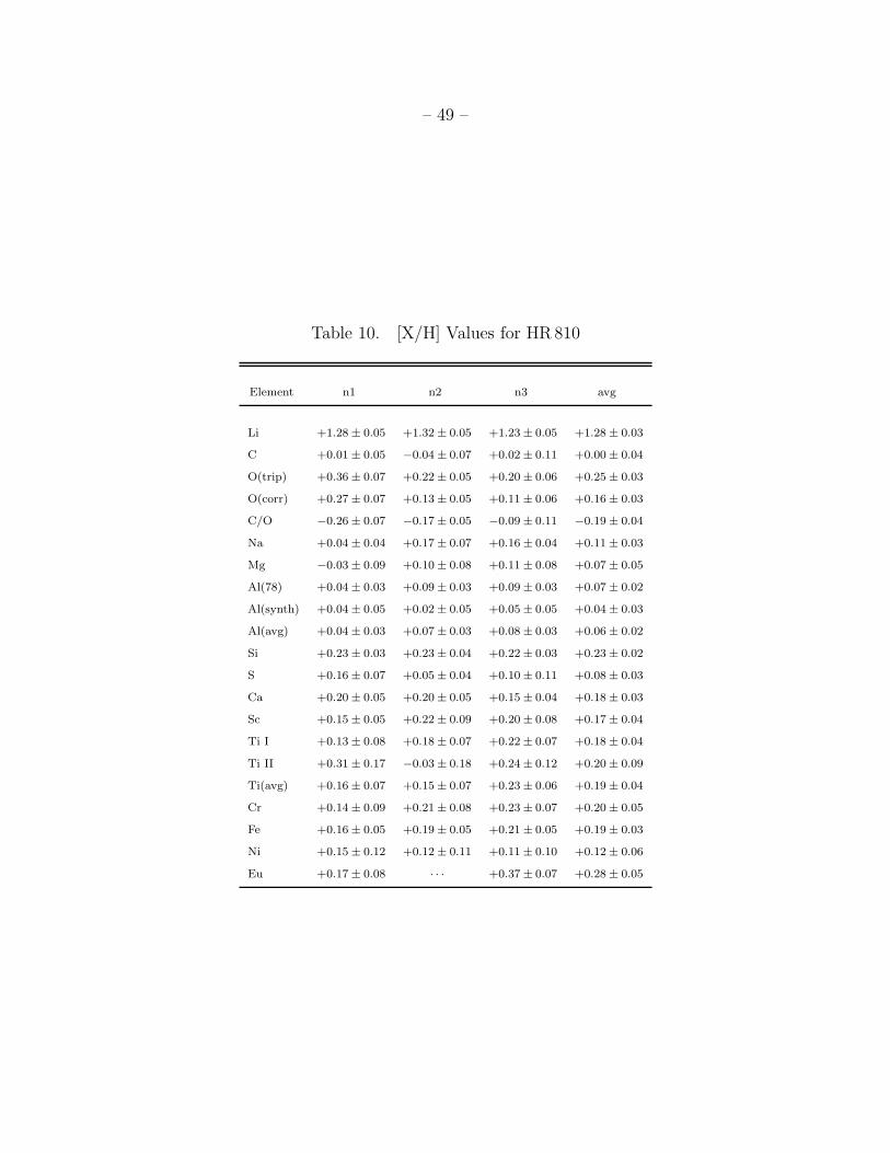
– 49 –

Table 10. [X/H] Values for HR810

Element n1 n2 n3 avg

Li +1.28 ± 0.05 +1.32 ± 0.05 +1.23 ± 0.05 +1.28 ± 0.03

C +0.01 ± 0.05 −0.04 ± 0.07 +0.02 ± 0.11 +0.00 ± 0.04

O(trip) +0.36 ± 0.07 +0.22 ± 0.05 +0.20 ± 0.06 +0.25 ± 0.03

O(corr) +0.27 ± 0.07 +0.13 ± 0.05 +0.11 ± 0.06 +0.16 ± 0.03

C/O −0.26 ± 0.07 −0.17 ± 0.05 −0.09 ± 0.11 −0.19 ± 0.04

Na +0.04 ± 0.04 +0.17 ± 0.07 +0.16 ± 0.04 +0.11 ± 0.03

Mg −0.03 ± 0.09 +0.10 ± 0.08 +0.11 ± 0.08 +0.07 ± 0.05

Al(78) +0.04 ± 0.03 +0.09 ± 0.03 +0.09 ± 0.03 +0.07 ± 0.02

Al(synth) +0.04 ± 0.05 +0.02 ± 0.05 +0.05 ± 0.05 +0.04 ± 0.03

Al(avg) +0.04 ± 0.03 +0.07 ± 0.03 +0.08 ± 0.03 +0.06 ± 0.02

Si +0.23 ± 0.03 +0.23 ± 0.04 +0.22 ± 0.03 +0.23 ± 0.02

S +0.16 ± 0.07 +0.05 ± 0.04 +0.10 ± 0.11 +0.08 ± 0.03

Ca +0.20 ± 0.05 +0.20 ± 0.05 +0.15 ± 0.04 +0.18 ± 0.03

Sc +0.15 ± 0.05 +0.22 ± 0.09 +0.20 ± 0.08 +0.17 ± 0.04

Ti I +0.13 ± 0.08 +0.18 ± 0.07 +0.22 ± 0.07 +0.18 ± 0.04

Ti II +0.31 ± 0.17 −0.03 ± 0.18 +0.24 ± 0.12 +0.20 ± 0.09

Ti(avg) +0.16 ± 0.07 +0.15 ± 0.07 +0.23 ± 0.06 +0.19 ± 0.04

Cr +0.14 ± 0.09 +0.21 ± 0.08 +0.23 ± 0.07 +0.20 ± 0.05

Fe +0.16 ± 0.05 +0.19 ± 0.05 +0.21 ± 0.05 +0.19 ± 0.03

Ni +0.15 ± 0.12 +0.12 ± 0.11 +0.11 ± 0.10 +0.12 ± 0.06

Eu +0.17 ± 0.08 · · · +0.37 ± 0.07 +0.28 ± 0.05

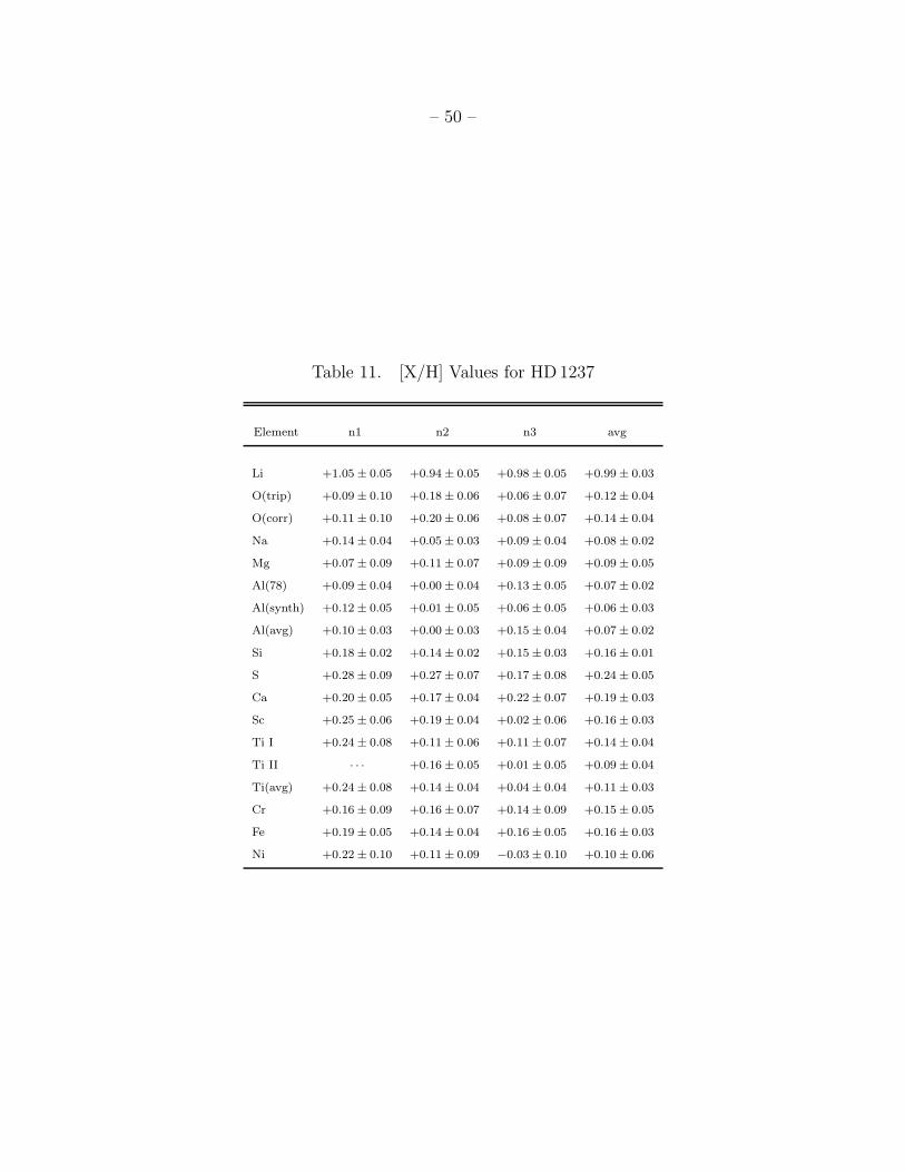
– 50 –

Table 11. [X/H] Values for HD 1237

Element n1 n2 n3 avg

Li +1.05 ± 0.05 +0.94 ± 0.05 +0.98 ± 0.05 +0.99 ± 0.03

O(trip) +0.09 ± 0.10 +0.18 ± 0.06 +0.06 ± 0.07 +0.12 ± 0.04

O(corr) +0.11 ± 0.10 +0.20 ± 0.06 +0.08 ± 0.07 +0.14 ± 0.04

Na +0.14 ± 0.04 +0.05 ± 0.03 +0.09 ± 0.04 +0.08 ± 0.02

Mg +0.07 ± 0.09 +0.11 ± 0.07 +0.09 ± 0.09 +0.09 ± 0.05

Al(78) +0.09 ± 0.04 +0.00 ± 0.04 +0.13 ± 0.05 +0.07 ± 0.02

Al(synth) +0.12 ± 0.05 +0.01 ± 0.05 +0.06 ± 0.05 +0.06 ± 0.03

Al(avg) +0.10 ± 0.03 +0.00 ± 0.03 +0.15 ± 0.04 +0.07 ± 0.02

Si +0.18 ± 0.02 +0.14 ± 0.02 +0.15 ± 0.03 +0.16 ± 0.01

S +0.28 ± 0.09 +0.27 ± 0.07 +0.17 ± 0.08 +0.24 ± 0.05

Ca +0.20 ± 0.05 +0.17 ± 0.04 +0.22 ± 0.07 +0.19 ± 0.03

Sc +0.25 ± 0.06 +0.19 ± 0.04 +0.02 ± 0.06 +0.16 ± 0.03

Ti I +0.24 ± 0.08 +0.11 ± 0.06 +0.11 ± 0.07 +0.14 ± 0.04

Ti II · · · +0.16 ± 0.05 +0.01 ± 0.05 +0.09 ± 0.04

Ti(avg) +0.24 ± 0.08 +0.14 ± 0.04 +0.04 ± 0.04 +0.11 ± 0.03

Cr +0.16 ± 0.09 +0.16 ± 0.07 +0.14 ± 0.09 +0.15 ± 0.05

Fe +0.19 ± 0.05 +0.14 ± 0.04 +0.16 ± 0.05 +0.16 ± 0.03

Ni +0.22 ± 0.10 +0.11 ± 0.09 −0.03 ± 0.10 +0.10 ± 0.06

– 51 –

Table 12. [X/H] Values from Keck Spectra

Element HD12661 HD 16141 HD37124 HD38529 HD 46375 HD52265 HD92788 HD177830 BD -10

C +0.29 ± 0.05 +0.08 ± 0.05 −0.10 ± 0.05 +0.24 ± 0.06 +0.31 ± 0.07 +0.20 ± 0.04 +0.24 ± 0.05 · · ·

Na +0.33 ± 0.04 +0.03 ± 0.04 −0.39 ± 0.05 +0.34 ± 0.06 +0.20 ± 0.06 +0.24 ± 0.04 +0.28 ± 0.05 · · · +0.37

Mg +0.02 ± 0.04 +0.07 ± 0.05 −0.25 ± 0.05 +0.28 ± 0.07 · · · +0.20 ± 0.04 +0.13 ± 0.05 · · ·

Si +0.34 ± 0.01 +0.13 ± 0.03 −0.22 ± 0.02 +0.35 ± 0.03 +0.24 ± 0.01 +0.27 ± 0.02 +0.28 ± 0.01 +0.40 ± 0.06 +0.36

S +0.26 ± 0.10 +0.06 ± 0.05 −0.16 ± 0.06 +0.38 ± 0.15 · · · +0.11 ± 0.03 +0.13 ± 0.08 · · ·

Ca +0.33 ± 0.03 +0.14 ± 0.02 −0.24 ± 0.03 +0.31 ± 0.04 +0.23 ± 0.05 +0.27 ± 0.02 +0.27 ± 0.03 +0.38 ± 0.09 +0.32

Ti I +0.31 ± 0.05 +0.14 ± 0.05 −0.20 ± 0.06 +0.32 ± 0.07 +0.22 ± 0.07 +0.28 ± 0.03 +0.25 ± 0.04 +0.34 ± 0.13 +0.24

Ti II +0.37 ± 0.04 +0.20 ± 0.03 −0.20 ± 0.04 +0.35 ± 0.06 · · · +0.25 ± 0.05 +0.29 ± 0.04 · · ·

Ti(avg) +0.35 ± 0.03 +0.18 ± 0.03 −0.20 ± 0.03 +0.34 ± 0.05 +0.22 ± 0.07 +0.27 ± 0.03 +0.27 ± 0.03 +0.34 ± 0.13 +0.24

Cr +0.30 ± 0.04 +0.10 ± 0.06 −0.44 ± 0.05 +0.34 ± 0.07 +0.17 ± 0.08 · · · +0.29 ± 0.05 · · · +0.39

Fe +0.35 ± 0.02 +0.15 ± 0.02 −0.41 ± 0.03 +0.37 ± 0.04 +0.21 ± 0.04 +0.28 ± 0.02 +0.31 ± 0.03 +0.36 ± 0.05 +0.33

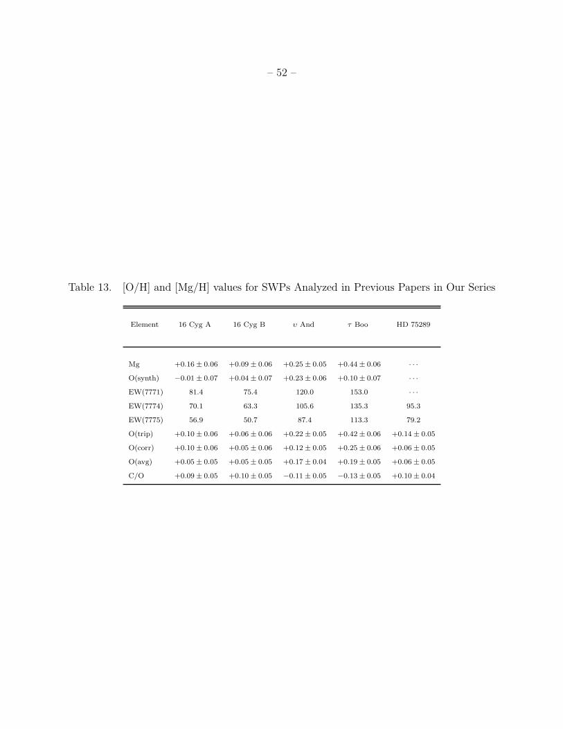
– 52 –

Table 13. [O/H] and [Mg/H] values for SWPs Analyzed in Previous Papers in Our Series

Element 16 Cyg A 16 Cyg B υ And τ Boo HD 75289

Mg +0.16 ± 0.06 +0.09 ± 0.06 +0.25 ± 0.05 +0.44 ± 0.06 · · ·

O(synth) −0.01 ± 0.07 +0.04 ± 0.07 +0.23 ± 0.06 +0.10 ± 0.07 · · ·

EW(7771) 81.4 75.4 120.0 153.0 · · ·

EW(7774) 70.1 63.3 105.6 135.3 95.3

EW(7775) 56.9 50.7 87.4 113.3 79.2

O(trip) +0.10 ± 0.06 +0.06 ± 0.06 +0.22 ± 0.05 +0.42 ± 0.06 +0.14 ± 0.05

O(corr) +0.10 ± 0.06 +0.05 ± 0.06 +0.12 ± 0.05 +0.25 ± 0.06 +0.06 ± 0.05

O(avg) +0.05 ± 0.05 +0.05 ± 0.05 +0.17 ± 0.04 +0.19 ± 0.05 +0.06 ± 0.05

C/O +0.09 ± 0.05 +0.10 ± 0.05 −0.11 ± 0.05 −0.13 ± 0.05 +0.10 ± 0.04

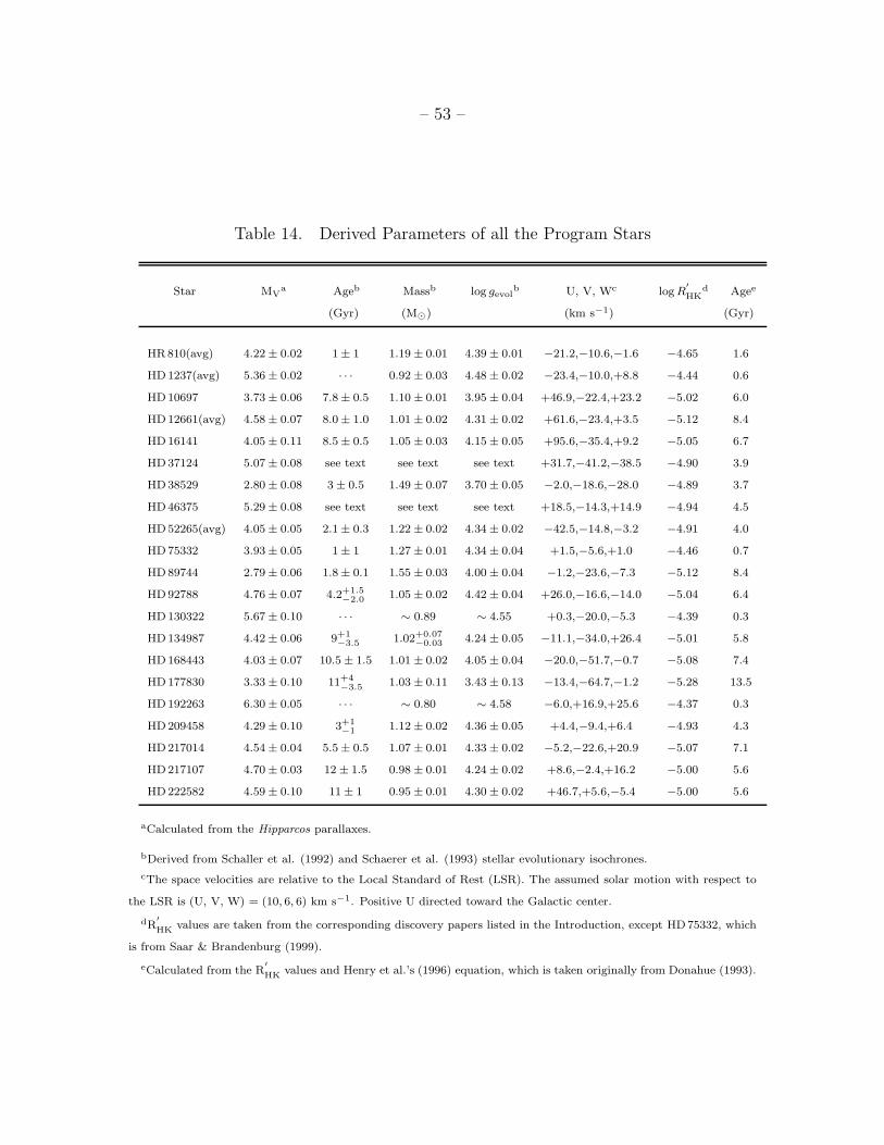
– 53 –

Table 14. Derived Parameters of all the Program Stars

Star MVa Ageb Massb log gevol

b U, V, Wc log R′

HKd Agee

(Gyr) (M⊙) (km s−1) (Gyr)

HR810(avg) 4.22 ± 0.02 1 ± 1 1.19 ± 0.01 4.39 ± 0.01 −21.2,−10.6,−1.6 −4.65 1.6

HD1237(avg) 5.36 ± 0.02 · · · 0.92 ± 0.03 4.48 ± 0.02 −23.4,−10.0,+8.8 −4.44 0.6

HD10697 3.73 ± 0.06 7.8 ± 0.5 1.10 ± 0.01 3.95 ± 0.04 +46.9,−22.4,+23.2 −5.02 6.0

HD12661(avg) 4.58 ± 0.07 8.0 ± 1.0 1.01 ± 0.02 4.31 ± 0.02 +61.6,−23.4,+3.5 −5.12 8.4

HD16141 4.05 ± 0.11 8.5 ± 0.5 1.05 ± 0.03 4.15 ± 0.05 +95.6,−35.4,+9.2 −5.05 6.7

HD37124 5.07 ± 0.08 see text see text see text +31.7,−41.2,−38.5 −4.90 3.9

HD38529 2.80 ± 0.08 3 ± 0.5 1.49 ± 0.07 3.70 ± 0.05 −2.0,−18.6,−28.0 −4.89 3.7

HD46375 5.29 ± 0.08 see text see text see text +18.5,−14.3,+14.9 −4.94 4.5

HD52265(avg) 4.05 ± 0.05 2.1 ± 0.3 1.22 ± 0.02 4.34 ± 0.02 −42.5,−14.8,−3.2 −4.91 4.0

HD75332 3.93 ± 0.05 1 ± 1 1.27 ± 0.01 4.34 ± 0.04 +1.5,−5.6,+1.0 −4.46 0.7

HD89744 2.79 ± 0.06 1.8 ± 0.1 1.55 ± 0.03 4.00 ± 0.04 −1.2,−23.6,−7.3 −5.12 8.4

HD92788 4.76 ± 0.07 4.2+1.5−2.0

1.05 ± 0.02 4.42 ± 0.04 +26.0,−16.6,−14.0 −5.04 6.4

HD130322 5.67 ± 0.10 · · · ∼ 0.89 ∼ 4.55 +0.3,−20.0,−5.3 −4.39 0.3

HD134987 4.42 ± 0.06 9+1−3.5

1.02+0.07−0.03

4.24 ± 0.05 −11.1,−34.0,+26.4 −5.01 5.8

HD168443 4.03 ± 0.07 10.5 ± 1.5 1.01 ± 0.02 4.05 ± 0.04 −20.0,−51.7,−0.7 −5.08 7.4

HD177830 3.33 ± 0.10 11+4

−3.51.03 ± 0.11 3.43 ± 0.13 −13.4,−64.7,−1.2 −5.28 13.5

HD192263 6.30 ± 0.05 · · · ∼ 0.80 ∼ 4.58 −6.0,+16.9,+25.6 −4.37 0.3

HD209458 4.29 ± 0.10 3+1−1

1.12 ± 0.02 4.36 ± 0.05 +4.4,−9.4,+6.4 −4.93 4.3

HD217014 4.54 ± 0.04 5.5 ± 0.5 1.07 ± 0.01 4.33 ± 0.02 −5.2,−22.6,+20.9 −5.07 7.1

HD217107 4.70 ± 0.03 12 ± 1.5 0.98 ± 0.01 4.24 ± 0.02 +8.6,−2.4,+16.2 −5.00 5.6

HD222582 4.59 ± 0.10 11 ± 1 0.95 ± 0.01 4.30 ± 0.02 +46.7,+5.6,−5.4 −5.00 5.6

aCalculated from the Hipparcos parallaxes.

bDerived from Schaller et al. (1992) and Schaerer et al. (1993) stellar evolutionary isochrones.

cThe space velocities are relative to the Local Standard of Rest (LSR). The assumed solar motion with respect to

the LSR is (U, V, W) = (10, 6, 6) km s−1. Positive U directed toward the Galactic center.

dR′

HKvalues are taken from the corresponding discovery papers listed in the Introduction, except HD75332, which

is from Saar & Brandenburg (1999).

eCalculated from the R′

HKvalues and Henry et al.’s (1996) equation, which is taken originally from Donahue (1993).

– 54 –

Table 15. Composition of Earth Relative to Solar Photospherea

Element Ratio [X/Fe]⊕

C/Fe −4.21

O/Fe −0.79

Na/Fe −0.56

Mg/Fe −0.05

Al/Fe +0.00

Si/Fe −0.09

Ca/Fe +0.00

Ti/Fe −0.05

aFor the purposes

of calculating the numbers in

this table, we adopted the solar

phospheric abundances listed

by Grevesse & Sauval (1998).

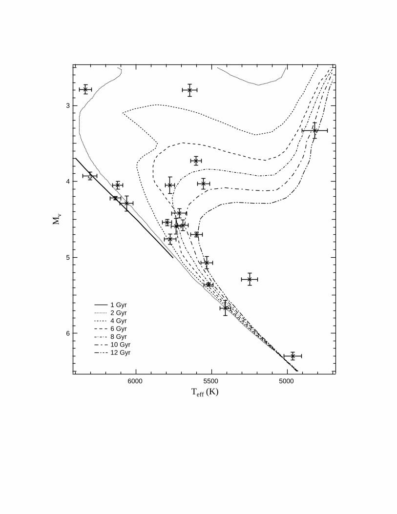
6

5

4

3

Mv

6000 5500 5000

Teff (K)

1 Gyr 2 Gyr 4 Gyr 6 Gyr 8 Gyr 10 Gyr 12 Gyr

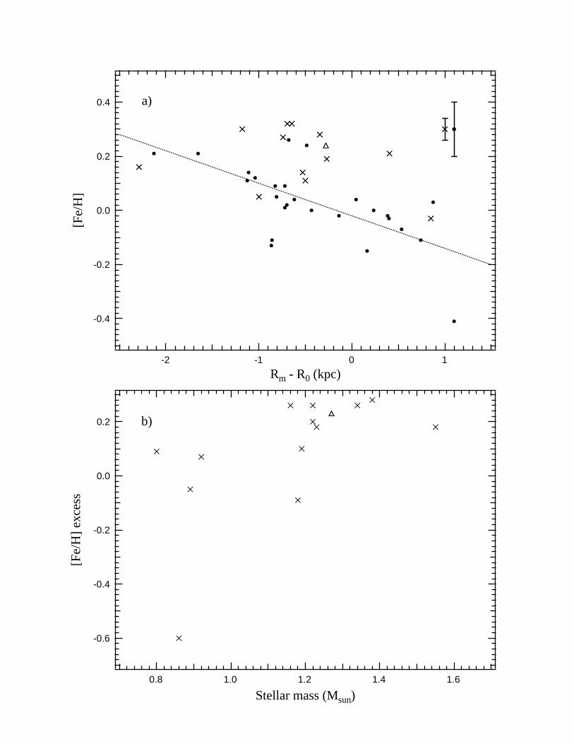
-0.4

-0.2

0.0

0.2

0.4

[Fe/

H]

-2 -1 0 1

Rm - R0 (kpc)

a)

-0.6

-0.4

-0.2

0.0

0.2

[Fe/

H]

exce

ss

1.61.41.21.00.8

Stellar mass (Msun)

b)

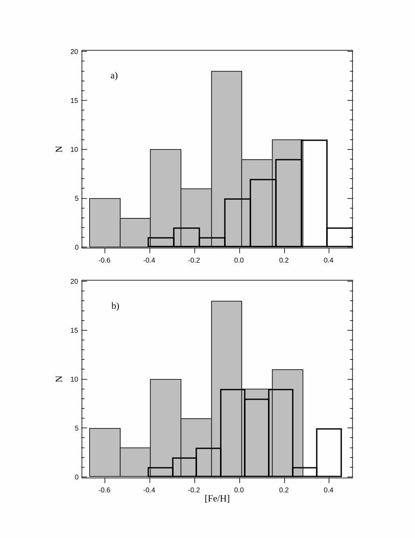
20

15

10

5

0

N

-0.6 -0.4 -0.2 0.0 0.2 0.4

a)

20

15

10

5

0

N

-0.6 -0.4 -0.2 0.0 0.2 0.4[Fe/H]

b)

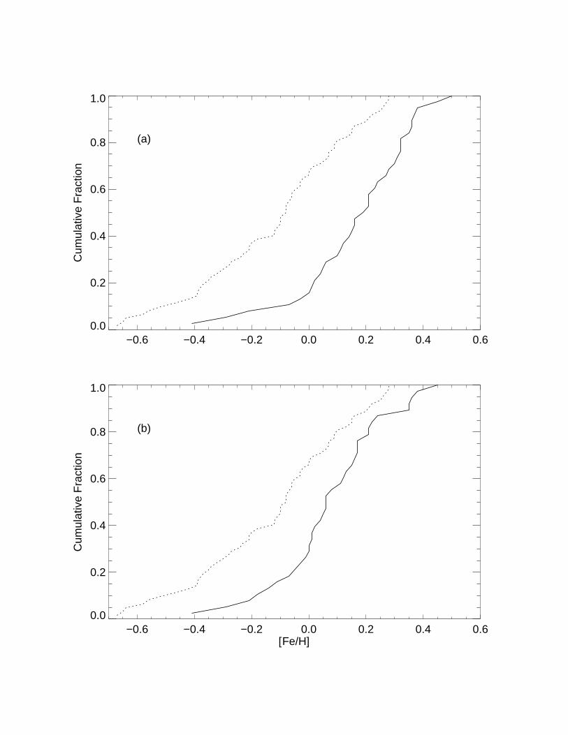
−0.6 −0.4 −0.2 0.0 0.2 0.4 0.60.0

0.2

0.4

0.6

0.8

1.0

Cum

ulat

ive

Fra

ctio

n

(a)

−0.6 −0.4 −0.2 0.0 0.2 0.4 0.6[Fe/H]

0.0

0.2

0.4

0.6

0.8

1.0

Cum

ulat

ive

Fra

ctio

n

(b)

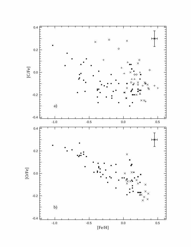
-0.4

-0.2

0.0

0.2

0.4[C

/Fe]

-1.0 -0.5 0.0 0.5

a)

-0.4

-0.2

0.0

0.2

0.4

[O/F

e]

-1.0 -0.5 0.0 0.5

[Fe/H]

b)

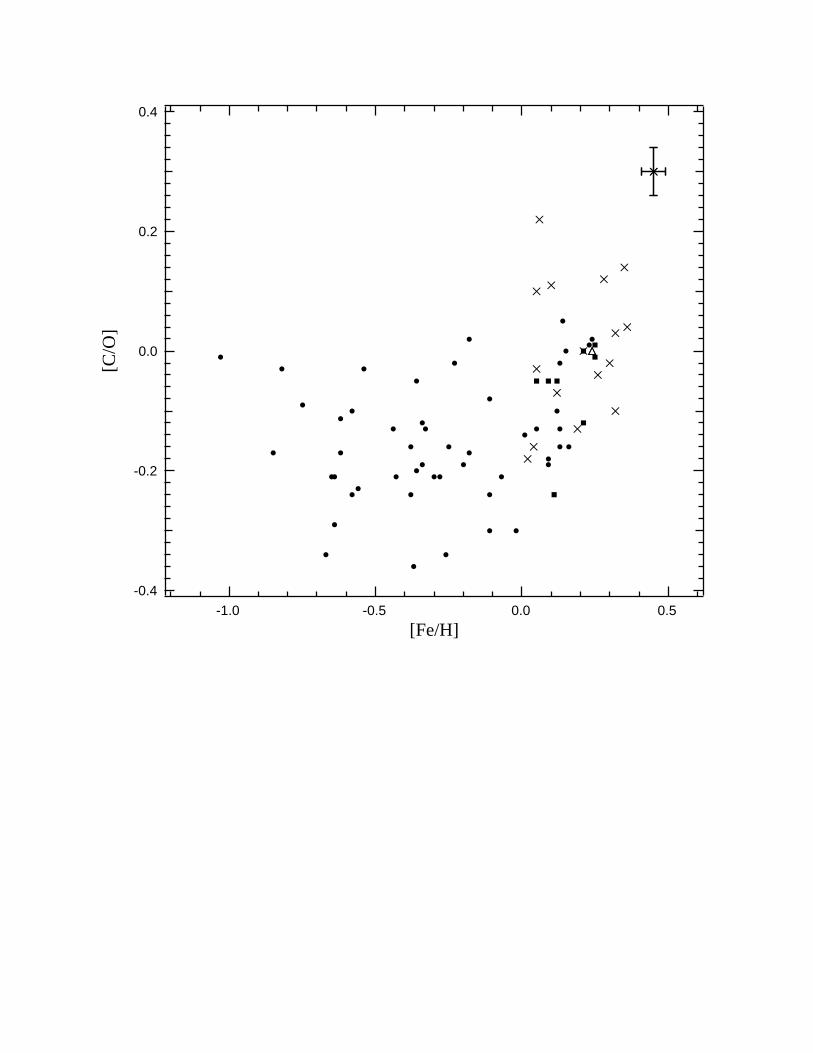
-0.4

-0.2

0.0

0.2

0.4[C

/O]

-1.0 -0.5 0.0 0.5

[Fe/H]

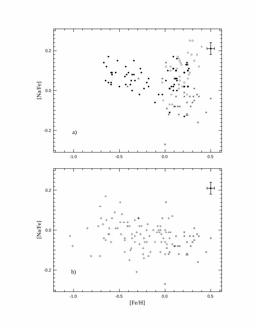
-0.2

0.0

0.2

[Na/

Fe]

-1.0 -0.5 0.0 0.5

[Fe/H]

b)

-0.2

0.0

0.2

[Na/

Fe]

-1.0 -0.5 0.0 0.5

a)

0.4

0.2

0.0

-0.2

[Mg/

Fe]

-1.0 -0.5 0.0 0.5

[Fe/H]

b)

0.4

0.2

0.0

-0.2

[Mg/

Fe]

-1.0 -0.5 0.0 0.5

a)

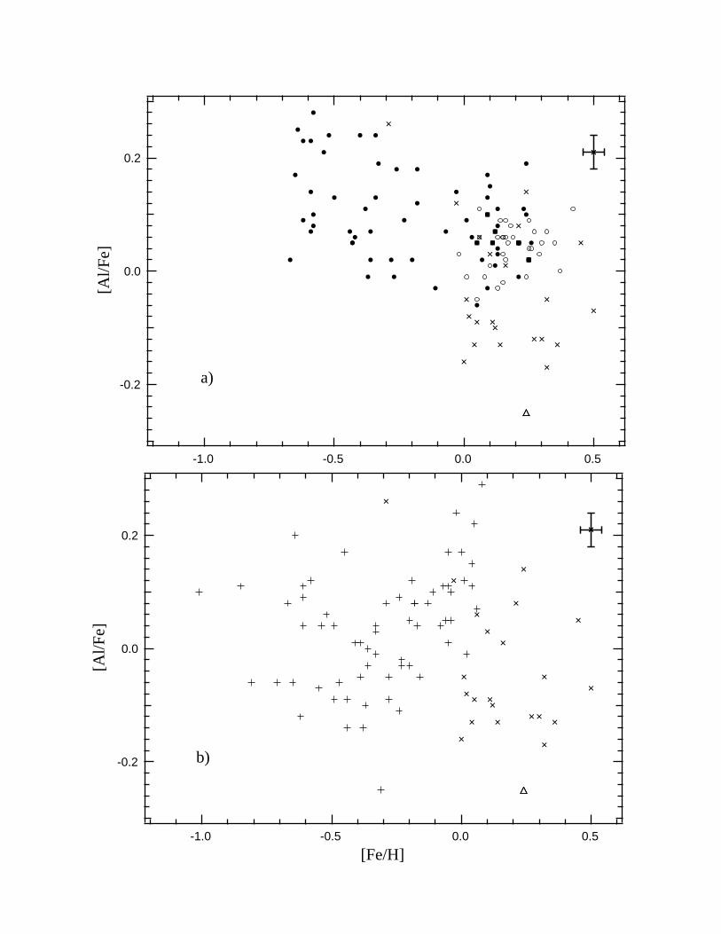
-0.2

0.0

0.2

[Al/F

e]

-1.0 -0.5 0.0 0.5

a)

-0.2

0.0

0.2

[Al/F

e]

-1.0 -0.5 0.0 0.5

[Fe/H]

b)

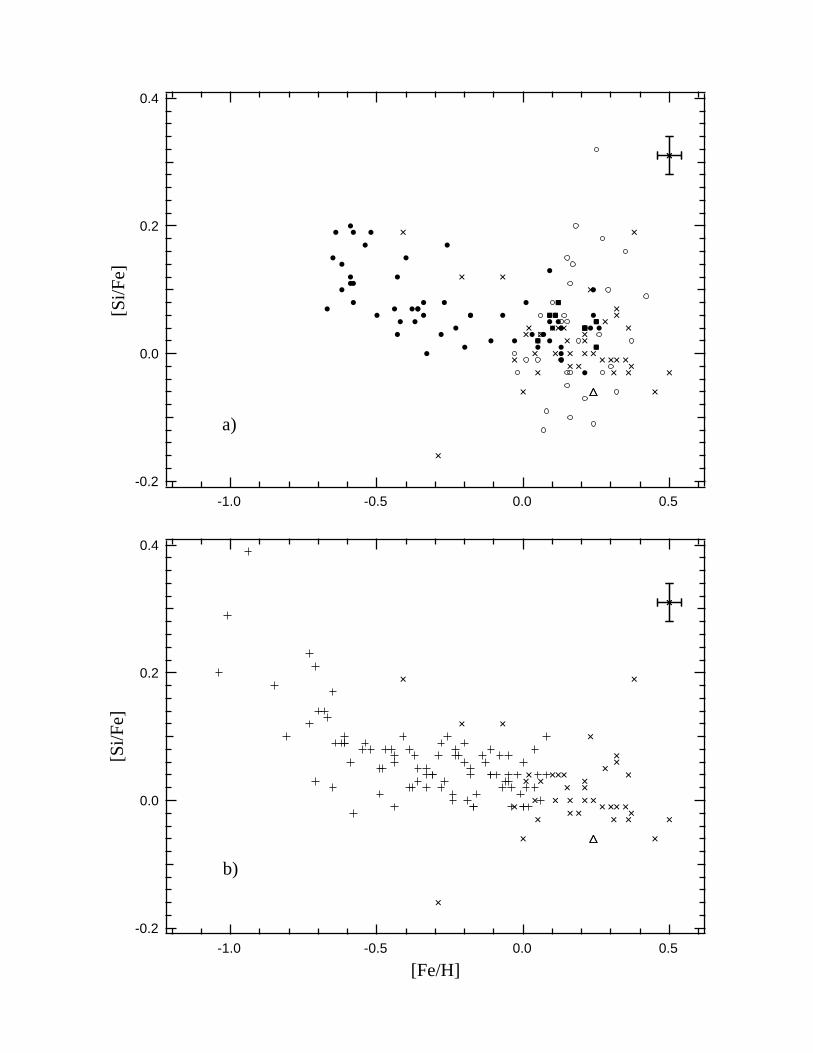
0.4

0.2

0.0

-0.2

[Si/F

e]

-1.0 -0.5 0.0 0.5

[Fe/H]

b)

0.4

0.2

0.0

-0.2

[Si/F

e]

-1.0 -0.5 0.0 0.5

a)

0.4

0.2

0.0

-0.2

[Ca/

Fe]

-1.0 -0.5 0.0 0.5

a)

0.4

0.2

0.0

-0.2

[Ca/

Fe]

-1.0 -0.5 0.0 0.5

[Fe/H]

b)

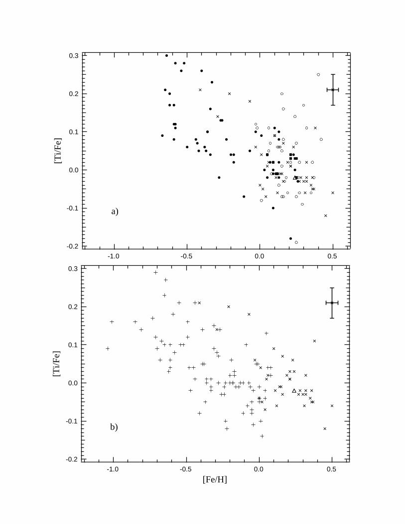
0.3

0.2

0.1

0.0

-0.1

-0.2

[Ti/F

e]

-1.0 -0.5 0.0 0.5

a)

0.3

0.2

0.1

0.0

-0.1

-0.2

[Ti/F

e]

-1.0 -0.5 0.0 0.5

[Fe/H]

b)