HAL Id: hal-00457392https://hal.archives-ouvertes.fr/hal-00457392

Submitted on 15 Oct 2021

HAL is a multi-disciplinary open accessarchive for the deposit and dissemination of sci-entific research documents, whether they are pub-lished or not. The documents may come fromteaching and research institutions in France orabroad, or from public or private research centers.

L’archive ouverte pluridisciplinaire HAL, estdestinée au dépôt et à la diffusion de documentsscientifiques de niveau recherche, publiés ou non,émanant des établissements d’enseignement et derecherche français ou étrangers, des laboratoirespublics ou privés.

Distributed under a Creative Commons Attribution| 4.0 International License

Interpreting the yield of transit surveys: are theregroups in the known transiting planets population?

F. Fressin, T. Guillot, Lionel Nesta

To cite this version:F. Fressin, T. Guillot, Lionel Nesta. Interpreting the yield of transit surveys: are there groups in theknown transiting planets population?. Astronomy and Astrophysics - A&A, EDP Sciences, 2009, 504,pp.605-615. �10.1051/0004-6361/200810097�. �hal-00457392�

A&A 504, 605–615 (2009)DOI: 10.1051/0004-6361/200810097c© ESO 2009

Astronomy&

Astrophysics

Interpreting the yield of transit surveys:are there groups in the known transiting planets population?�

F. Fressin1, T. Guillot1, and L. Nesta2

1 Observatoire de la Côte d’Azur, Laboratoire Cassiopée, CNRS UMR 6202, BP 4229, 06304 Nice cedex 4, Francee-mail: ffressin@cfa.harvard.edu

2 Observatoire Français des Conjonctures Économiques (OFCE), 250 rue Albert Einstein, 06560 Valbonne, France

Received 30 April 2008 / Accepted 24 December 2008

ABSTRACT

Context. Each transiting planet discovered is characterized by 7 measurable quantities, that may or may not be linked. This includesthose relative to the planet (mass, radius, orbital period, and equilibrium temperature) and those relative to the star (mass, radius,effective temperature, and metallicity). Correlations between planet mass and period, surface gravity and period, planet radius andstar temperature have been previously observed among the 31 known transiting giant planets. Two classes of planets have beenpreviously identified based on their Safronov number.Aims. We use the CoRoTlux transit surveys to compare simulated events to the sample of discovered planets and test the statisticalsignificance of these correlations. Using a model proved to be able to match the yield of OGLE transit survey, we generate a largesample of simulated detections, in which we can statistically test the different trends observed in the small sample of known transitingplanets.Methods. We first generate a stellar field with planetary companions based on radial velocity discoveries, use a planetary evolutionmodel assuming a variable fraction of heavy elements to compute the characteristics of transit events, then apply a detection criterionthat includes both statistical and red noise sources. We compare the yield of our simulated survey with the ensemble of 31 well-characterized giant transiting planets, using different statistical tools, including a multivariate logistic analysis to assess whether thesimulated distribution matches the known transiting planets.Results. Our results satisfactorily match the distribution of known transiting planet characteristics. Our multivariate analysis showsthat our simulated sample and observations are consistent to 76%. The mass vs. period correlation for giant planets first observed withradial velocity holds with transiting planets. The correlation between surface gravity and period can be explained as the combinedeffect of the mass vs. period lower limit and by the decreasing transit probability and detection efficiency for longer periods and highersurface gravity. Our model also naturally explains other trends, like the correlation between planetary radius and stellar effectivetemperature. Finally, we are also able to reproduce the previously observed apparent bimodal distribution of planetary Safronovnumbers in 10% of our simulated cases, although our model predicts a continuous distribution. This shows that the evidence for theexistence of two groups of planets with different intrinsic properties is not statistically significant.

Key words. methods: statistical – techniques: photometric – planets and satellites: formation – planetary systems –planetary systems: formation

1. Introduction

The number of giant transiting exoplanets discovered is increas-ing rapidly and amounts to 32 at the date of this writing. Theability to measure the masses and radii of these objects providesus with a unique possibility to determine their composition andto test planet formation models. Although uncertainties on stel-lar and planetary characteristics do not allow the determinationof the precise composition of planets individually, much can belearned from a global, statistical approach.

A particularly intriguing observation made by Hansen &Barman (2007) from an examination of the 18 first transitingplanets is the apparent grouping of objects in two categoriesbased on their Safronov number.

The Safronov number θ is defined as:

θ =12

[Vesc

Vorb

]2=

aRp

Mp

M�, (1)

� Appendix is only available in electronic form athttp://www.aanda.org

where Vesc is the escape velocity from the surface of the planetand Vorb is the orbital velocity of the planet around its host star,a is the semi-major axis, Mp and M� are the respective mass ofthe planet and its host star, and Rp is the radius of the planet. Itis indicative of the efficiency with which a planet scatters otherbodies, and could play an important role in understanding pro-cesses that affected planet formation.

If real, this division into two groups would probably implythe existence of different formation or accretion mechanisms, oralternatively require revised evolution models.

Other puzzling observations include the possible trends be-tween planet mass and orbital period (Mazeh et al. 2005; Gaudiet al. 2005) and between gravity and orbital period (Southworthet al. 2007, first mentioned by Noyes in 2006).

The importance of transit detections biases has been pointedout by Gaudi (2005) and Pont et al. (2006) ; they have detailedthe relation between the detection criterion, the characteristicsof the astrophysical targets and the observational characteristicsof surveys. In a previous article (Fressin et al. 2007, hereafterPaper I), we presented CoRoTlux, a tool to statistically model a

Article published by EDP Sciences

606 F. Fressin et al.: Groups within transiting exoplanets?

population of stars and planets and compare it to the ensemble ofdetected transiting planets. We showed the results to be in verygood agreement with the 14 planets known at that time.

In the present article, we examine whether these trends andgroups can be explained in the framework of our model orwhether they imply the existence of more complex physicalmechanisms for the formation or evolution of planets that arenot included in present models. We first describe our modeland an updated global statistical analysis of the results includ-ing 17 newly discovered planets (Sect. 2). We then examine thetrends between mass, gravity and orbital period (Sect. 3), thegrouping in terms of planetary radius and stellar effective tem-perature (Sect. 4), and the grouping in terms of Safronov number(Sect. 5).

2. Method and result update

2.1. Principle of the simulations

As described in more detail in Paper I, the generation of a pop-ulation of transiting planets with CoRoTlux involves the follow-ing steps:

1. we generate a population of stars from the Besançon catalog(Robin et al. 2003);

2. Stellar companions (doubles, triples) are added using fre-quencies of occurrence and period distributions based onDuquennoy & Mayor (1991);

3. planetary companions with random orbital inclinations aregenerated with a frequency of occurrence that depends onthe host star metallicity with the relation derived by Santoset al. (2004). The parameters of the planets (period, mass, ec-centricity) are derived by cloning the known radial-velocity(hereafter RV) list of planets 1. We consider only planetsabove 0.3 times the mass of Jupiter, which yields a list of229 objects. This mass cut-off is chosen from radial veloc-ity analysis (Fischer & Valenti 2005), as their planetary oc-currence relation is considered unbiased down to this limit.Because of a strong bias of transit surveys towards extremelyshort orbital periods P (less than 2 days), we add to the listclones drawn from the short-orbit planets found from tran-siting surveys. The probabilities are adjusted so that on av-erage ∼3 transit-planet clones with P ≤ 2 days are added tothe RV list of 229 giant planets. This number is obtained bymaximum likelihood on the basis of the OGLE survey to re-produce both the planet populations at very short periods thatare not constrained by RV measurements and the ones withlonger periods that are discovered by both types of surveys(see Paper I);

4. we compute planetary radii using a structure and evolutionmodel that is adjusted to fit the radius distribution of knowntransiting planets: the planetary core mass is assumed to bea function of the stellar metallicity, and the evolution is cal-culated by including an extra heat source term equal to 1%of the incoming stellar heat flux (Guillot et al. 2006; Guillot2008)2;

5. we determine which transiting planets are detectable, givenan observational duty cycle and a level of white and red noiseestimated a posteriori (Pont et al. 2006). We also use a cut-off in stellar effective temperature Teff,cut above which weconsider that it will be too difficult for RV techniques to

1 we use Schneider’s planet encyclopaedia: www.exoplanets.eu2 An electronic version of the table of simulated planets used to extrap-olate radii is available at www.obs-nice.fr/guillot/pegasids/

confirm an event. We choose Teff,cut = 7200 K as a fiducialvalue. This value is an estimate of the limit for Teff used bythe OGLE follow-up group (Pont, pers. communication); inpractice it has little consequences on the results.

In order to analyze the complete yield of transit discoveries prop-erly, we should simulate each successful survey (OGLE: e.g.see Udalski 2003; HATnet: e.g. see Bakos et al. 2006; TrES:e.g. see Alonso et al. 2004; SWASP: e.g. see Collier Cameronet al. 2006; XO: e.g. see McCullough et al. 2006) one by one.However, we take advantage of the fact that these differentground-based surveys have similar observation biases and simi-lar noise levels (e.g. the red noise level for SWASP (Smith et al.2006) is close to the one of OGLE (Pont et al. 2006), althoughtheir instruments and target magnitude range are different). Asa consequence, one can notice that in terms of transit depth andperiod distribution of detected transiting planets, these surveysachieve very similar performances. Therefore, as in Paper I, webase our model parameters (stellar fields, duty cycle, red noiselevel) on OGLE parameters (Udalski 2003; Bouchy et al. 2004;Pont et al. 2005).

2.2. The known transiting giant planets

Our results will be systematically compared to the sampleof 31 transiting giant planets that are known at the date of thiswriting. These include in particular:

– 22 planets for which the refined parameters based on the uni-form analysis of transit light curves and the observable prop-erties of the host stars have been updated by Torres et al.(2008). We exclude the sub-giant Hot Neptune GJ-436 b thatdoes not fit our mass criterion and is undetectable by currentground-based surveys.

– 9 planets recently discovered and not included in Torreset al. (2008). The characteristics of these planets have notbeen refined and are to be considered with more caution.Among these planets, we added the first two discoveriesof the CoRoT satellite. Although CoRoT has significantlyhigher photometric precision and is better suited to findlonger period planets than ground based surveys, we in-cluded both CoRoT-Exo-1b (Barge et al. 2008) and CoRoT-Exo-2b (Alonso et al. 2008) in our analysis, as they are thetwo deepest planet candidates of the initial run of the satelliteand have similar periods and transit depths to planets discov-ered from ground-based surveys.

The characteristics of the transiting planets are shown in Tables 1and 2 for their host stars. These tables are used to test our model.Where the stellar metallicity is unknown, we arbitrarily used so-lar metallicity (see below and the appendix for a discussion).

2.3. A new metallicity distribution for stars hosting planets

In Paper I, we had concluded that the metallicity distributionof stars with Pegasids (planets with masses between 0.3 and15 MJup and periods P < 10 days) was significantly differentfrom those of stars with planets having longer orbital periods.This was based on three facts:

– the list of radial-velocity planets known showed a lack ofgiant planets with short orbital periods around metal-poorstars. Among 25 Pegasids, none were orbiting stars with[Fe/H] < −0.07, contrary to planets on longer orbits foundalso around metal-poor stars;

F. Fressin et al.: Groups within transiting exoplanets? 607

Table 1. Characteristics of transiting planets included in this study.

Name Mp Rp P T i a Reference[MJup] [RJup] [days] [JD − 2 450 000] [◦] [AU]

HD17156b 3.13 ± 0.21 1.21 ± 0.12 21.21691 ± _71 4374.8338 ± _20 86.5+1.1−0.7 0.15 [Barbieri07]Fischer07/Irwin08

HD147506b�� 8.04 ± 0.40 0.98 ± 0.04 5.63341 ± _13 4212.8561 ± _6 >86.8 0.0685 [Bakos07]Winn07*HD149026b 0.36 ± 0.03 0.71 ± 0.05 2.8758882 ± _61 4272.7301 ± _13 90 ± 3.1 0.0432 [Sato05]Winn07*HD189733b 1.15 ± 0.04 1.154 ± 0.017 2.218581 ± _2 3931.12048 ± _2 85.68 ± 0.04 0.031 [Bouchy05]Pont07*HD209458b 0.657 ± 0.006 1.320 ± 0.025 3.52474859 ± _38 2826.628521 ± _87 86.929 ± 0.010 0.047 [Charbonneau00]Winn05/Knutson06*TrES − 1 0.76 ± 0.05 1.081 ± 0.029 3.0300737 ± _26 3186.80603 ± _28 >88.4 0.0393 [Alonso04]Sozzetti04/Winn07*TrES − 2 1.198 ± 0.053 1.220+.045

−.042 2.47063 ± _1 3957.6358 ± _10 83.90 ± 0.22 0.0367 [ODonovan06] Sozzetti07*TrES − 3 1.92 ± 0.23 1.295 ± 0.081 1.30619 ± _1 4185.9101 ± _3 82.15 ± 0.21 0.0226 [ODonovan07]*TrES − 4 0.84 ± 0.20 1.674 ± 0.094 3.553945 ± _75 4230.9053 ± _5 82.81 ± 0.33 0.0488 [Mandushev07]*XO − 1b 0.90 ± 0.07 1.184+.028

−.018 3.941534 ± _27 3887.74679 ± _15 89.36+.46−.53 0.0488 [McCullough06]Holman06*

XO − 2b 0.57 ± 0.06 0.973+.03−.008 2.615838 ± _8 4147.74902 ± _20 >88.35 0.037 [Burke07]*

XO − 3b 13.25 ± 0.64 1.1−2.1 3.19154 ± 14 4025.3967 ± _38 79.32 ± 1.36 0.0476 [Johns-Krull08]HAT − P − 1b 0.53 ± 0.04 1.203 ± 0.051 4.46529 ± _9 3997.79258 ± _24 86.22 ± 0.24 0.0551 [Bakos07]Winn07*HAT − P − 3b 0.599 ± 0.026 0.890 ± 0.046 2.899703 ± 54 4218.7594 ± _29 87.24 ± 0.69 0.0389 [Torres07]*HAT − P − 4b 0.68 ± 0.04 1.27 ± 0.05 3.056536 ± _57 4245.8154 ± _3 89.9+0.1

−2.2 0.0446 [Kovacs07]*HAT − P − 5b 1.06 ± 0.11 1.26 ± 0.05 2.788491 ± _25 4241.77663 ± _22 86.75 ± 0.44 0.0407 [Bakos07]*HAT − P − 6b 1.057 ± 0.119 1.330 ± 0.061 3.852985 ± _5 4035.67575 ± _28 85.51 ± 0.35 0.0523 [Noyes07]*WASP − 1b 0.867 ± 0.073 1.443 ± 0.039 2.519961 ± _18 4013.31269 ± _47 >86.1 0.0382 [Cameron06]Shporer06/Charbonneau06*WASP − 2b 0.81 − 0.95 1.038 ± 0.050 2.152226 ± _4 4008.73205 ± 28 84.74 ± 0.39 0.0307 [Cameron06]Charbonneau06*WASP − 3b 1.76 ± 0.11 1.31+.07

−.14 1.846834 ± _2 4143.8503 ± _4 84.4+2.1−0.8 0.0317 [Pollacco07]

WASP − 4b 1.27 ± 0.09 1.45+.04−.08 1.338228 ± _3 4365.91475 ± _25 87.54+2.3

−.04 0.023 [Wilson08]WASP − 5b 1.58 ± 0.11 1.090+.094

−.058 1.6284296 ± _42 4375.62466 ± _26 >85.0 0.0268 [Anderson08]COROT − Exo − 1b 1.03 ± 0.12 1.49 ± 0.08 1.5089557 ± _64 4159.4532 ± _1 85.1 ± 0.5 0.025 [Barge08]COROT − Exo − 2b 3.31 ± 0.16 1.465 ± 0.029 1.7429964 ± _17 4237.53562 ± _14 87.84 ± 0.10 0.028 [Alonso08]OGLE − TR − 10b 0.61 ± 0.13 1.122+0.12

−0.07 3.101278 ± _4 3890.678 ± _1 87.2−90 0.0416 [Konacki05]Pont07/Holman07*OGLE − TR − 56b 1.29 ± 0.12 1.30 ± 0.05 1.211909 ± _1 3936.598 ± _1 81.0 ± 2.2 0.0225 [Konacki03]Torres04/Pont07*OGLE − TR − 111b 0.52 ± 0.13 1.01 ± 0.04 4.0144479 ± _41 3799.7516 ± _2 88.1 ± 0.5 0.0467 [Pont04]Santos06/Winn06/Minniti07*OGLE − TR − 113b 1.32 ± 0.19 1.09 ± 0.03 1.4324757 ± _13 3464.61665 ± _10 88.8−90 0.0229 [Bouchy04]Bouchy04/Gillon06*OGLE − TR − 132 1.14 ± 0.12 1.18 ± 0.07 1.689868 ± _3 3142.5912 ± _3 81.5 ± 1.6 0.0299 [Bouchy04]Gillon07*OGLE − TR − 182b 1.01 ± 0.15 1.13+.24

−.08 3.97910 ± _1 4270.572 ± _2 85.7 ± 0.3 0.051 [Pont08]OGLE − TR − 211b 1.03 ± 0.20 1.36+.18

−.09 3.67724 ± _3 3428.334 ± _3 >82.7 0.051 [Udalski07]

Underscores indicate uncertainties on last printed digits. Bracket = announcement paper. No bracket = reference from which most parameters have been chosen from. *=also in Torres et al.(2008).MJup = 1.8986112 × 1030 g is the mass of Jupiter. RJup = 71, 492 km is Jupiter’s equatorial radius.

References: Charbonneau et al. (2000); Konacki et al. (2003); Bouchy et al. (2004); Pont et al. (2004); Torres et al. (2004); Alonso et al. (2004); Sozzetti et al. (2004); Sato et al. (2005);Bouchy et al. (2005); Winn et al. (2005); O’Donovan et al. (2006); Collier Cameron et al. (2006); Knutson et al. (2007); Gillon et al. (2006); Charbonneau et al. (2006); Holman et al.(2006); Shporer et al. (2007); Winn et al. (2007b,c); Bakos et al. (2007); Burke et al. (2007); O’Donovan et al. (2007); Mandushev et al. (2007); Torres et al. (2007); Pont et al. (2008);Gillon et al. (2007); Minniti et al. (2007); Winn et al. (2007a); Kovács et al. (2007).The table is derived from Frederic Pont’s web site: http://www.inscience.ch/transits/.�� HD147056 is also called HAT-P-2.

– the list of transiting planets also showed a lack of planetsaround metal-poor stars, with stellar metallicities rangingfrom −0.03 to 0.37 ([−0.08, 0.44] with error bars);

– the population of transiting planets generated withCoRoTlux was found to systematically underpredictstellar metallicities compared to the sample of observedtransiting planet. The period vs. metallicity diagram thusformed was found to be 2.9σ away from the maximumlikelihood of the simulated planet position in the diagram(see Paper I)3.On the other hand, a similar calculation done by splittingthe RV list in a low-metallicity part ([Fe/H] < −0.07) and ahigh-metallicity part (with two different period distributionsfor simulated planets as a function of their host star metal-licity) would end in a period vs. metallicity diagram in good

3 Paper I shows how we estimate the deviation of real planets from themaximimum likelihood of the model: in each 2-parameter space, we binour data on a 20 × 20 grid as a compromise between resolution of themodels and characteristic variations of the parameters. The probabilityof an event in each bin is considered equal to the normalized numberof draws in that bin in our large model sample. The likelihood of a31-planet draw is the sum of the logarithms of the individual probabli-ties of its events. We estimate the standard deviation of 1000 random31-event draws among the model detection sample, and calculate thedeviation from maximum likelihood of the known planets as a functionof this standard deviation.

agreement with the observations (0.4σ from the maximumlikelihood).

On the basis of an additional 51 RV giant planets and 17 tran-siting planets discovered since Paper I, we must now reexam-ine this conclusion. Indeed, the average metallicity of stars har-boring transiting planets has evolved. The OGLE survey wascharacterized by a surprisingly high value ([Fe/H] = 0.24).The planets discovered since have significantly lower metallic-ities (an average of [Fe/H] = 0.07). Finally, TrES-2, TrES-3,XO-3, HAT-P-6 and CoRoT-Exo-1 all appear to have metallici-ties lower than −0.07.

In Paper I, the metallicity distribution of simulated starswas based on that extracted from the photometric observationof the solar neighborhood of the Geneva-Copenhagen survey(Nordström et al. 2004). This metallicity distribution is in factcentred one dex lower (−0.14 instead of −0.04) than the oneobserved using spectrometry by RV surveys (Fischer & Valenti2005; Santos et al. 2004). Since the latter two works are usedto derive the frequency of stars bearing planets, we now chooseto also use these for the metallicity distribution of stars in ourfields. More specifically, our metallicity distribution law and theplanet occurrence rate are obtained by combining the Santoset al. (2004) and the Fischer & Valenti (2005) surveys. Figure 1shows the metallicity distribution and planet occurrence that re-sult directly from these hypotheses.

As a consequence, we find that with this improved distri-bution of stellar metallicities with the new sample of observed

608 F. Fressin et al.: Groups within transiting exoplanets?

Table 2. Characteristics of stars hosting the transiting planets included in this study

Name Vmag M� R� Teff [Fe/H] Reference[M�] [R�] [K]

HD17156 8.2 1.2 ± 0.1 1.47 ± 0.08 6079 ± 56 0.24 ± 0.03 Fischer07/Irwin08HD147506 8.7 1.32 ± 0.08 1.48 ± 0.05 6290 ± 110 0.12 ± 0.08 Bakos07/Winn07*HD149026 8.2 1.3 ± 0.06 1.45 ± 0.1 6147 ± 50 0.36 ± 0.05 Sato05/Winn07*HD189733 7.7 0.82 ± 0.03 0.755 ± 0.011 5050 ± 50 −0.03 ± 0.04 Bouchy05/Pont07*HD209458 7.7 1.101 ± 0.064 1.125 ± 0.022 6117 ± 26 0.02 ± 0.03 Sozzetti04/Knutson06*TrES − 1 11.8 0.89 ± 0.035 0.811 ± 0.020 5250 ± 75 −0.02 ± 0.06 Sozzetti04,06/Winn07*TrES − 2 11.4 0.98 ± 0.062 1.000+.036

−.033 5850 ± 50 −0.15 ± 0.10 Sozzetti07*TrES − 3 12.4 0.90 ± 0.15 0.802 ± 0.046 5720 ± 150 O Donovan07*TrES − 4 11.6 1.22 ± 0.17 1.738 ± 0.092 6100 ± 150 Mandushev07*XO − 1 11.5 1.0 ± 0.03 0.928 ± 0.015 5750 ± 13 0.015 ± 0.03 MCCullough06/Holman06*XO − 2 11.2 0.98 ± 0.02 0.964+.02

−.009 5340 ± 32 0.45 ± 0.02 Burke07*XO − 3 9.8 1.41 ± 0.08 1.377 ± 0.083 6429 ± 50 −0.18 ± 0.03 Johns-Krull07HAT − P − 1 10.4 1.12 ± 0.09 1.115 ± 0.043 5975 ± 45 0.13 ± 0.02 Bakos07/Winn07*HAT − P − 3 11.9 0.936+.036

−.062 0.824+.043−.035 5185 ± 46 0.27 ± 0.04 Torres07*

HAT − P − 4 11.2 1.26+.06−.14 1.59 ± 0.07 5860 ± 80 0.24 ± 0.08 Kovacs07*

HAT − P − 5 12.0 1.160 ± 0.062 1.167 ± 0.049 5960 ± 100 0.24 ± 0.15 Bakos07*HAT − P − 6 10.4 1.29 ± 0.06 1.46 ± 0.06 6570 ± 80 −0.13 ± 0.08 Noyes07*WASP − 1 11.8 1.15+.24

−.09 1.453 ± 0.032 6110 ± 45 0.23 ± 0.08 Cameron06 Charbonneau06/Stempels07*WASP − 2 12.0 0.79+.15

−.04 0.813 ± 0.032 5200 ± 200 Cameron06/Charbonneau06*WASP − 3 10.5 1.24+.06

−.11 1.31+.05−.12 6400 ± 100 0.0 ± 0.2 Pollacco07

WASP − 4 12.5 0.90 ± 0.08 0.95+.05−.03 5500 ± 150 0.0 ± 0.2 Wilson08

WASP − 5 12.3 0.97 ± 0.09 1.026+.073−.044 5700 ± 150 0.0 ± 0.2 Anderson08

COROT − Exo − 1 13.6 0.95 ± 0.15 1.11 ± 0.05 5950 ± 150 −0.3 ± 0.25 Barge08COROT − Exo − 2 12.57 0.97 ± 0.06 0.902 ± 0.018 5625 ± 120 ∼ 0 Alonso08/Bouchy08OGLE − TR − 10 15.8 1.10 ± 0.05 1.14+0.11

−0.6 6075 ± 86 0.28 ± 0.10 Santos06/Pont07*OGLE − TR − 56 16.6 1.17 ± 0.04 1.32 ± 0.06 6119 ± 62 0.19 ± 0.07 Santos06/Pont07*OGLE − TR − 111 17.0 0.81 ± 0.02 0.83 ± 0.03 5044 ± 83 0.19 ± 0.07 Santos06/Winn06*OGLE − TR − 113 16.1 0.78 ± 0.02 0.77 ± 0.02 4804 ± 106 0.15 ± 0.10 Santos06/Gillon06*OGLE − TR − 132 16.9 1.26 ± 0.03 1.34 ± 0.08 6210 ± 59 0.37 ± 0.07 Gillon07*OGLE − TR − 182 17 1.14 ± 0.05 1.14+.23

−.06 5924 ± 64 0.37 ± 0.08 Pont08OGLE − TR − 211 15.5 1.33 ± 0.05 1.64+.21

−.05 6325 ± 91 0.11 ± 0.10 Udalski07

Underscores indicate uncertainties on last printed digits. *=also in Torres et al. (2008).References: Charbonneau et al. (2000); Konacki et al. (2003); Bouchy et al. (2004); Pont et al. (2004); Torres et al. (2004); Alonso et al. (2004); Sozzetti et al. (2004); Sato et al. (2005);Bouchy et al. (2005); Winn et al. (2005); O’Donovan et al. (2006); Collier Cameron et al. (2006); Knutson et al. (2007); Gillon et al. (2006); Charbonneau et al. (2006); Holman et al.(2006); Shporer et al. (2007); Winn et al. (2007b,c); Bakos et al. (2007); Burke et al. (2007); O’Donovan et al. (2007); Mandushev et al. (2007); Torres et al. (2007); Pont et al. (2008);Gillon et al. (2007); Minniti et al. (2007); Winn et al. (2007a); Kovács et al. (2007); Bouchy et al. (2008); The discovery Papers are in brackets. The table is taken from Pont’s site: http://www.inscience.ch/transits/.

Fig. 1. Distribution of stars as a function of their metallicity [Fe/H].Upper panel: fraction of stars with planets as a function of their metal-licity, as obtained from radial velocity surveys (Santos et al. 2004;Fischer & Valenti 2005). Bottom panel: normalized distribution of stel-lar metallicities assumed in Paper I (blue) and in this work (black). Theresulting [Fe/H] distribution of planet-hosting stars is also shown in red.

planets alleviates the need to advocate a distinction in metallici-ties between stars harboring short-period giant planets and starsthat harbor planets on longer periods. Quantitatively, our newmetallicity vs. period diagram is at 1.09σ of the maximum like-lihood. We therefore conclude that, contrary to Paper I, thereis no statistically significant bias between the planet periodicityand the stellar metallicity in the observed exoplanet sample.

2.4. Statistical evaluation of the performances of the model

As shown in detail in the appendix (see online version), themodel is evaluated using univariate, two-dimensional and multi-variate statistical tests. Specifically, we show that the parametersfor the simulated and observed planets globally have the samemean and standard deviation and that both Student-t tests andKolmogorov-Smirnov tests indicate that the two populations arestatistically indistinguishable. However, while these univariatetests provide preliminary tests of the quality of the data, theyare not sufficient because of the multiple correlations betweenparameters of the problem.

Table 3 presents the Pearson correlation coefficients betweeneach variable. It shows that the problem indeed possesses multi-ple, complex correlations. In this table, the variable Y character-izes the “reality” of the planet considered (it is equal to 1 if theplanet of the list is an observed one, and to 0 if it is a simulatedplanet). We see that Y is very weakly correlated with parametersof the problem. This indicates that the model is well-behaved,but does not constitute a complete validity test in itself.

Table 4 presents the results of a multivariate test using a so-called logistic regression (see the appendix for more details).This method allows us to include simultaneously all planet char-acteristics as predictors of the probability of being a known tran-siting planet (hereafter named “real” planets as opposed to sim-ulated ones), thereby controlling for the correlations between allvariables at once. Based on the maximum likelihood estimationmethod, it provides information on whether a given characteriticis positively (resp. negatively) and significantly (resp. non sig-nificantly) related to the fact of being a real planet. Moreover,

F. Fressin et al.: Groups within transiting exoplanets? 609

Table 3. Pearson correlations between planetary and stellar characteristics. Significant correlations (≥0.5) are boldfaced.

Y� θ [Fe/H] Teff R� M� Teq P Rp Mp

θ −0.0046[Fe/H] 0.0048 0.0560

Teff −0.0013 −0.1300 −0.0227R� 0.0006 0.1240 −0.0283 0.8103M� 0.0003 −0.1301 −0.0237 0.9359 0.8761Teq 0.0006 −0.1411 −0.0013 0.7338 0.7605 0.7380P −0.0029 0.4184 0.0068 −0.0304 −0.0280 −0.0303 −0.3990Rp 0.0015 −0.3038 −0.5129 0.4833 0.5203 0.5030 0.5191 −0.1931Mp −0.0046 0.6560 0.0676 −0.0317 −0.0318 −0.0324 −0.0476 −0.3250 −0.1457

�: Variable Y has value 1 if the planet is observed, 0 if it is simulated.

Table 4. Logistic maximum likelihood estimates.

Variable β̂ t-stat. PM� 0.467 0.63 0.528

[Fe/H] 0.415 1.39 0.164Teff –0.517 –0.81 0.417R� 0.059 0.12 0.901P –0.235 –0.32 0.746

Mp 0.329 0.35 0.726Rp 0.305 0.90 0.370Teq –0.296 –0.46 0.648θ –0.904 –0.58 0.563

Maximum likelihood estimations.Probability Pχ2 = 0.756.β̂ is indicative of a correlation with Y ; “t-stat” is the the distance instandard deviations from no correlation, and P represents the probabil-ity that the model and observations are not significantly different.

it computes the probability Pχ2 as a general assessment of thequality of the fit. In our case, a large Pχ2 implies no significantdifference between the simulated and real planets. Globally, thegeneral fit of the model shows that simulated planets are not sig-nificantly distinct from real planets (Pχ2 = 0.765). This can becompared to a model in which model radii are artificially in-creased by 10%, for which Pχ2 ∼ 10−4 (see appendix).

Table 4 also presents for each seven independent variablesof the problem plus the planet equilibrium temperature Teq andSafronov number θ how a given variable is correlated with thefact that a planet is “real” (as opposed to being one of the simu-lated planets in the list). The different statistical parameters pre-sented in this table are defined in the appendix. We only providehere a short description: β̂ is indicative of a correlation between agiven variable and the Y (reality) variable. “t-stat” represent thedistance from the mean in terms of standard deviations (student-ttest). P represents the probability that the correlation is signif-icant. The two last parameters are evaluated using a bootstrapmethod.

The fact that the parameters β̂ in Table 4 are non-zero indi-cate that there is a correlation between each parameter and thevariable Y. However, the t-student test indicates that in everycase but one (for [Fe/H]), the values obtained for β̂ are consis-tent with 0 to within one standard deviation: the agreement be-tween model and observations is good. This is further shown bythe high P values (indicative of consistency between model andobservations): The lowest P value is associated with the stellarmetallicty [Fe/H], but it is high enough not to show a statisti-cally significant difference between our modeled sample and real

observations. However, this characteristic is the one with thelargest error bars, and the only one with missing data (for TrES-3, TrES-4, WASP-2 and CoRoT-Exo-2). We included [Fe/H], asit is an important feature of our model, in our multivariate anal-ysis, but the comparison with real planets for this characteristicis to be considered carefully. The quality of the agreement be-tween observed planet characteristics and our model improvesto 88.4% if we remove [Fe/H] from our logistic maximum like-lihood estimates (see the appendix for details and further tests).

2.5. Updated mass-radius diagram

Throughout this paper, we will use density maps of the simu-lated detections and compare them to the observations. Thesedensity maps use a resolution disk template to obtain smoothplots. The size of the resolution template is a function of thenumber of events present in the diagram. The color levels fol-low a linear density rule for most diagrams we show. In the caseof specific diagrams showing rare long period discoveries (morethan 5 days) and large surface gravity or Safronov number, wechoose to use a logarithmic color range for density maps to em-phasize these rare events. A probability map is established us-ing the model detection sample (50 000 detections obtained bysimulating the number of observations from the OGLE survey)multiple times. Again, we stress that we limited our model toplanets below 0.3 MJup, both because the question of the compo-sition becomes more important and complex for small planets,and because RV detection biases are also more significant ; theirdistribution is only partially known from RV surveys.

Figure 2 shows the mass-radius diagram density map simu-lated with CoRoTlux and compared to the known planets. Gapsin the diagram at ∼3 MJup and ∼6−7 MJup are due to the smallsample of close-in RV planets in these ranges and the fact thatour mass distribution is obtained by cloning these observed plan-ets rather than relying on a smooth distribution (see Paper I fora discussion). These gaps should disappear with more discover-ies of close-in planets by RV. Otherwise, the model distributionand the known planets are in fairly good agreement, as indicatedby the 1.7 ∼ 1.8σ distance to the maximum likelihood for thisdiagram (Table 9). However, the agreement is not as good asone would expect, probably because of two planets with espe-cially large radii, CoRoT-Exo-2b and TrES-4b. The existence ofthese planets is a problem for evolution models in general thatgoes beyond the present statistical tests that we propose in thisarticle.

610 F. Fressin et al.: Groups within transiting exoplanets?

Fig. 2. Mass – radius relation for the transiting Pegasids discovered todate (filled circles for planets with low Safronov number θ < 0.05, opencircles for planets with higher θ values). The joint probability densitymap obtained from our simulation is shown as grey contours (or colorcontours in the electronic version of the article). The resolution disksize used for the contour plot appears in the bottom left part of the pic-ture. At a given (x, y) location the normalized joint probability densityis defined as the number of detected planets in the resolution disk cen-tered on (x, y) divided by the maximum number of detected planets in aresolution disk anywhere on the figure.

Fig. 3. Mass-period distribution of known short-period exoplanets.Crosses correspond to non-transiting planets discovered by radial-velocity surveys. Open and filled circles correspond to transiting planets(with Safronov numbers below and over 0.05, respectively).

3. Trends between mass, surface gravity and orbitalperiod

3.1. A correlation between mass and orbital periodof Pegasids

Figure 3 compares the known radial-velocity planets to the onesdetected in transit. The figure highlights the fact that transit sur-veys are clearly biased towards detecting short-period planets.However, as shown in Paper I and furthermore reinforced in thepresent study, the two populations are perfectly compatible pro-vided a limited proportion of very small planets (P < 2 days) isadded.

Mazeh et al. (2005) had pointed out the possibility of an in-triguing correlation between the masses and periods of the sixfirst known transiting exoplanets. Figure 3 shows that the trendis confirmed with the present sample of planets. This correlationmay be due to a migration rate that is inherently dependant upon

Fig. 4. Planetary surface gravity versus orbital period of transiting giantplanets discovered to date (circles) compared to a simulated joint prob-ability density map (contours). Symbols and density plot are the sameas in Fig. 2.

planetary mass or to other formation mechanisms. It is not thepurpose of this paper to analyze this correlation. However, be-cause we use clones of the radial-velocity planets in our model,it is important to stress that this absence of small-mass planetswith very short orbital distances can subtend some of the resultsthat will be discussed hereafter.

3.2. A correlation between surface gravity and orbital periodof Pegasids?

The existence of a possible anti-correlation between planetarysurface gravity g = GMp/R2

p and the orbital period of thenine first transiting planets has been considered for some time(Southworth et al. 2007). This correlation still holds (Fig. 4) forthe Pegasids with periods below 5 days and with jovian massesdiscovered to date. At the same time, it is important to stress thatmassive objects (XO-3b, HAT-P-2b and HD17156b) are clearoutliers (see Fig. 5): Their much larger surface gravity probablyimplies that they are in a different regime.

Our model agrees well with the observations (in this P − gdiagram real planets are at 0.51σ from maximum likelihood ofthe simulated results). We can explain the apparent correlationin Fig. 4 as stemming from the existence of two zones with fewdetectable transiting giant planets:

1. the bottom left part of the diagram where planets are rare,because of a lack of light planets (with low surface gravity)with short periods, as discussed in Sect. 3.1;

2. the upper right part of the diagram (high surface gravity, lowplanetary radius) where transiting planets are less likely totransit and more difficult to detect.

Figure 5 shows the same probability density map as in Fig. 4 butat a larger scale in period and gravity. The three outliers to the“correlation” appear. These are the large mass planets XO-3b,HAT-P-2b and HD17156b. Given the method chosen to draw theplanet population with CoRoTlux, the probability density func-tion that we derive is small, but non-zero around these objects,and also elsewhere in the diagram due to the presence of non-transiting giant planets with appropriate characteristics. Seen atthis larger scale, it is clear that the planetary-gravity vs. periodrelation is much more complex than a simple linear relation.

Globally, Figs. 4 and 5 indicate that the relation betweenplanet surface gravity and orbital period is not a consequence

F. Fressin et al.: Groups within transiting exoplanets? 611

Fig. 5. Same figure as Fig. 4 with extended surface gravity and periodranges. Note that the scale of the color levels is logarithmic, in order toemphasize the presence of outliers.

Table 5. Mean planet radius for cool versus hot stars.

Cool stars Hot starsTeff < 5400 K Teff ≥ 5400 K

“Real” planets 1.072 RJup 1.267 RJup

All simulated planets 1.058 RJup 1.202 RJup

Detectable simulated planets 1.074 RJup 1.251 RJup

of a link between the planet composition and its orbital period.Rather, we see it as a consequence of the correlation betweenplanetary mass and orbital period for short period giant planets,which is, as discussed in the previous section, probably linked tomass-dependent migration mechanisms.

4. A correlation between stellar effectivetemperature and planet radius ?

The range of radius of Pegasids is surprisingly large, especiallywhen one considers the difference in compositions (masses ofheavy elements varying from almost 0 to ∼100 M⊕) that arerequired to explain known transiting planets within the samemodel (Guillot et al. 2006; Guillot 2008). Our underlying planetcomposition/evolution model is based on the assumption of acorrelation of the stellar metallicity with the heavy element con-tent in the planet. We checked that no other variable is responsi-ble for a correlation that would affect this conclusion.

We present the results obtained in the Teff − Rp diagram asthey are the most interesting: the two variables indeed are pos-itively correlated. Furthermore, given that errors in the stellarparameters are the main sources of uncertainty in the planetaryradius determinations, one could suppose that a systematic errorin the stellar radius measurement as a function of its effectivetemperature could be the cause of the variation in the estimatedplanetary radii. If true, this may alleviate the need for extremevariations in composition. It would cast doubts on the stellarmetallicity vs. planetary heavy element content correlation.

As shown in Table 5, the mean radius of planets orbitingcool stars (Teff < 5400 K) is 1.072 RJup and it is 1.267 RJup forplanets orbiting hot stars (Teff ≥ 5400 K). Slightly smaller valuesare obtained in our simulation when considering all transitingplanets. However, the values obtained when considering only thedetectable transiting planets are in extremely good agreementwith the observations.

Fig. 6. Stellar effective temperature versus planetary radius of transitinggiant planets discovered to date (circles) compared to a simulated jointprobability density map (contours). The black line is the sliding aver-age of radii in the [−250K,+250K] effective temperature interval for allsimulated transiting planets (both below and over the detection thresh-old). The white line is the same average for the detectable planets in thesimulation. The symbols and density map are the same as in Fig. 2.

Figure 6 shows in more detail how stellar effective tempera-ture and planetary radius are linked. We interpret the correlationbetween the two as the combined effect of irradiation (visiblewith the plotted average radius of all planets with at least onetransit event in simulated light curves) and detection bias (visiblewith the plotted average radius of simulated planets detected):

1. the planets orbiting bright stars are more irradiated. Themean radius of a planet orbiting a warmer star is thus higherat a given period. This effect is taken into account in ourplanetary evolution model (see Guillot & Showman 2002;Guillot et al. 2006);

2. the detection of a planet of a given radius is easier for coolerstars since for main sequence stars effective temperature andstellar radius are positively correlated.

We therefore conclude that the effective temperature-planetaryradius correlation is a consequence of the physics of the problemrather than the cause of the spread in planetary radii. This impliesthat another explanation – an important variation in the planetarycomposition – is needed to account for the observed radii.

As in the mass-radius diagram (Fig. 2), there is an outlier atthe bottom of Fig. 6, HD149026b. As discussed previously, thisobject lies at the boundary of what we could simulate, both interms of masses and amounts of heavy elements, so that we donot consider this as significant. It is also presently not detectablefrom a transit survey. Clearly, with more sensitive transit sur-veys, the presence of low-mass planets with a large fraction ofheavy elements compared to hydrogen and helium will populatethe bottom part of this diagram.

A last secondary outcome of the study of this diagram con-cerns the possible existence of two groups of planets roughlyseparated by a Teff = 5400 K line. We find that the existence oftwo such groups separated by ∼200 K or more appears serendip-itously in our model in 10% of the cases and is therefore notstatistically significant.

612 F. Fressin et al.: Groups within transiting exoplanets?

5. Two classes of Hot Jupiters, based on theirSafronov numbers?

According to Hansen & Barman (2007), the 16 planets discov-ered at the time of their study show a bimodal distribution inSafronov numbers, half of the sample having Safronov numbersθ ∼ 0.07 (“class I”) while the other half is such that θ ∼ 0.04(“class II”). They also point out that the equilibrium tempera-tures of the two classes of planets differ, the class II planets be-ing on average hotter. This is potentially of great interest becausethe Safronov number is indicative of the efficiency with which aplanet scatters other bodies and therefore this division in twoclasses, if real, may tell us something about the processes thatshaped planetary systems.

5.1. No significant gap between two classes

Figure 7 shows how the situation has evolved with the new tran-siting giant planets discovered thus far: Although a few planetshave narrowed the gap between the two ensemble of planets, itis still present and located at a Safronov number θ ∼ 0.05. Thetwo classes also have mean equilibrium temperatures that differ.

On the other hand, our model naturally predicts a continu-ous distribution of Safronov numbers. A trend is found in whichplanets with high equilibrium temperatures tend to have lowerSafronov numbers, which is naturally explained by the fact thatequilibrium temperature and orbital distance are directly linked(remember that θ = (a/Rp) (Mp/M�)).

We find that our θ − Teq joint probability density functionis representative of the observed population, being at 0.68σfrom the maximum likelihood (see appendix). A K-S test on theSafronov number yields a distance between the observed andsimulated distributions of 0.163 and a corresponding probabil-ity for a good match of 0.38, a value that should be improved infuture models, but that shows that the two ensembles are statis-tically indistinguishable.

Figure 8 compares the histogram of the distribution ofSafronov number for simulated detections with the histogramof real events. Interestingly, although distributions seem differ-ent from the 0.05-scale histogram, with a gap appearing in the0.05−0.055 slots, they fit each other when using the 0.1-scalehistogram, more appropriate for this low-number statistics anal-ysis (7 intervals for 31 events).

Figure 9 shows the probability of obtaining a gap of a givensize between the Safronov numbers of two potential groups ofa random draw. 26 of the known transiting Pegasids have theirSafronov number between 0 and 0.1. Setting a minimum numberof 5 planets in each of two classes, we look for the largest gapbetween Safronov numbers of a random draw of 26 simulatedPegasids. For each one of the 10 000 Monte-Carlo draws amongthe model detections sample, we calculate how large the mostimportant difference is between successive Safronov numbers ofthe 26 random draws. We find that a gap of 0.0102 between twopotential groups is an uncommon event (10% of the cases, as 4%of the cases have gaps of this size, and a total of 6% of the caseshave larger gaps), yet it is not exceptionally rare. Consideringthe 7 planet/star characteristics and their many possible combi-nations, this level of “rarity” is not statistically significant.

It is also interesting to consider the few high-Safronov-number planets discovered as in Fig. 10. The different gaps inthe diagram are due to our mass vs. period reproductions ofRV planets that do not uniformly cover the space of parame-ters. The unpopulated part in the right edge of the density mapis due to the absence of massive planets in the [3, 15] MJup range

Fig. 7. Safronov number versus equilibrium temperature of transitinggiant planets discovered to date (circles) compared to a simulated jointprobability density map (contours). Open (resp. filled) circles corre-spond to class I (resp. class II) planets. The symbols and density mapare the same as in Fig. 2.

Fig. 8. Comparison of the distribution of Safronov number betweensimulated detections (Red) and real events (Black). Top: histogram with6 0.1-scale columns, Bottom: histogram with 12 0.05-scale columns.

at close orbit in the RV planets. The simulated detections at bothhigh Safronov number and equilibrium temperature correspondto simulated clones of the planet HD41004b, with its large massof 18 MJup and its very close-in period of 1.33 days.

5.2. No bimodal distribution visible in other diagrams.

When plotted as a function of different stellar (effective temper-ature, mass, radius) and planetary characteristics (mass, radius,period, equilibrium temperature), the two potential Safronovclasses do not differ in a significant way. When plotting oursimulated detections as a function of their Safronov number indifferent diagrams, the two groups formed by restricting ourmodel detection sample with a Safronov number cut-off setat 0.05 partly overlap each other in most diagrams. Here, wechoose to present the planetary mass vs. equilibrium tempera-ture diagram used to provide a clear separation between the twopopulations (Hansen & Barman 2007; Torres et al. 2008). Wepresent in Fig. 11 this diagram as an example of the partial over-lap of the class I and class II detected planets and probabilitydensity maps. Contrary to indications based on a smaller sam-ple of observations, there is no longer a clear separation in thisdiagram between class I and class II planets.

F. Fressin et al.: Groups within transiting exoplanets? 613

Fig. 9. Occurrence of the largest observed separation of Safronovnumbers between two “groups” selected from random draws amongthe model detections sample. The vertical line shows the separation(0.0102) between the two classes of planets as inferred from the ob-servational sample.

Fig. 10. Same as Fig. 7 but for a larger range of Safronov numbers. Notethat the scale of the color levels is logarithmic, in order to emphasizethe presence of outliers.

5.3. No correlation between metallicity and Safronovnumber/class.

Torres et al. (2008) showed that a significant difference couldbe observed between the metallicity distributions of the twoSafronov classes. The high-Safronov number class (class I, θ >0.05) had its host star metallicity centered on 0.0, and the low-Safronov number class (class II) was centered on 0.2. Theypointed out that the Safronov numbers for Class I planets showa decreasing trend with metallicity.

The two recent discoveries of CoRoT-Exo-1-b ([Fe/H] =−0.4 and θ = 0.038) and OGLE TR182-b ([Fe/H] = 0.37 andθ = 0.08) tend to contradict this argument. Considering the 31known giant planets, the mean metallicity of stars hosting class Iplanets is now [Fe/H] = 0.6, and it is 1.6 for class II plan-ets. Figure 12 shows that although the metallicity vs. Safronovnumber distribution of detections we simulate is a likely result(0.63σ from maximum likelihood), the potential anticorrelationbetween θ and host star [Fe/H] (pointed out by Torres et al.(2008)) for class I planets is not present in our simulation, whichshows a continouous density map.

Fig. 11. Planetary mass versus equilibrium temperature of transiting gi-ant planets discovered to date (circles) compared to a simulated jointprobability density map (contours). Top panel: the density map accountsonly for simulated planets with a Safronov number θ > 0.05 (class Iplanets). Bottom panel: the density map corresponds only to planetswith θ < 0.05 (class II planets). The symbols and density maps are thesame as in Fig. 2.

5.4. No significant gap between two Safronov numberclasses.

Our study has shown us that a separation between two groups ofplanets linked to their Safronov number is unlikely for at leasttwo reasons:

1. the separation between the two groups is marginal. It onlyappears in the Safronov number histogram if the resolutionof the histogram is high in comparison to the number ofevents sampled. The separation of ∼0.01 between two pos-sible Safronov classes has a non-negligible 10% probabil-ity of occurring serendipitously in our distribution, which isotherwise continuous. Considering the relatively numerousparameters (4 for the star, 3 linked to the planet) and theircombinations, such a division to two groups appears quitelikely to occur fortuitously for one such parameter;

2. the separation between the two classes is not present in anyfigures other than the ones involving the Safronov numberitself. This includes also the separation in metallicity vs. θwhich is not statistically significant, especially given recentdiscoveries of CoRoT-Exo-1b and OGLE-TR-182b.

On the other hand, we cannot formally rule out the existenceof these two groups of planets. We hence eagerly await otherobservations of transiting planets for further tests.

614 F. Fressin et al.: Groups within transiting exoplanets?

Fig. 12. Safronov number of transiting planets as a function of theirhost star metallicity. The density map with linear contours comes fromthe model detection sample. Open and filled circles are respectivelyclass I planets (with Safronov number over 0.05) and class II planets(with Safronov number below 0.05) Symbols and density plot are thesame as in Fig. 2.

6. Conclusions

We have presented a coherent model of a population of stars andplanets that matches within statistical errors the observations oftransiting planets performed thus far. Thanks to new observa-tions, we have improved on our previous model (Paper I). Inparticular, we now show that with slightly improved assump-tions about the metallicity of stars in the solar neighborhood, themetallicity of stars with transiting giant planets can be explainedwithout assuming any bias in period vs. metallicity.

In order to validate our model, we have used a series of uni-variate, bivariate and multivariate statistical tests. As the sampleof radial-velocimetry planets and of transiting planets grows, weenvision that with these tools we will be able to much better char-acterize the planet population in our Galaxy and its dependenceon the star population, and also test models of planet formationand evolution.

With the current sample of transiting planets, our modelprovides a very good match to the observations, both when con-sidering planetary and stellar parameters one by one or glob-ally. Our analysis has revealed that the parameters for the mod-eled planets are presently statistically indistinguishable from theobservations, although there may be room for improvement ofthe model. It should be noted that our underlying assumptionsfor the composition and evolution of planets and stellar popula-tions are relatively simple. With a larger statistical sample, testsof these assumptions will be possible and will place importantconstraints on the planet-star distribution in our galactic neigh-borhood. The CoRoT mission is expected to be very importantin that respect, especially given the careful determination of thecharacteristics of the stellar population that is being monitored.

Using this method, we have been able to analyze and ex-plain the different correlations observed between transiting plan-ets characteristics:

1. Mass vs. period: one of the first correlations observed amongthe planet/star characteristics was the mass vs. period rela-tion of close-in RV planets (Mazeh et al. 2005). Althoughour model does not explain it, we confirm with a sample thatis now 4 times larger than at the time of the publication re-porting a lack of low-mass planets (Mp < 1MJup) with veryshort periods (P < 2 days).

2. Surface gravity vs. period: there is an inverse correlation be-tween the surface gravity and period of transiting planets. Weshow that this correlation is caused by the above mass vs. pe-riod effect, and by a lower detection probability for planetswith longer periods and higher surface gravities.

3. Radius vs. stellar effective temperature: planets around starswith higher effective temperatures tend to have larger sizes.This is naturally explained by a combination of slower con-traction due to the larger irradiation and by the increased dif-ficulty in finding planets around hotter, larger stars.

4. Safronov number: Hansen & Barman (2007); Torres et al.(2008) have identified a separation between two classes ofplanets, based on their Safrononov number, and visible indifferent diagrams (θ vs. Teq and vs. [Fe/H], Mp vs. Teq).With recent discoveries, this separation is still present in theSafronov number distribution, but no longer in other dia-grams. On the other hand, our simulation predicts distribu-tions that are continuous, in particular in terms of Safronovnumber. With this continuous distribution, we show that arandom draw of 30 simulated planets produces two spuriousgroups separated in Safronov number by a distance equal toor larger than the observations in 30% of the cases. The sep-aration is not visible and significant between the two classesin any other diagram we plotted. Therefore, we conclude thatthe separation to two classes is not statistically significant butis to be checked again with a larger sample of observed plan-ets. Interestingly, if on the contrary two classes of Safronovnumbers were found to exist we would have to revise ourmodel for the composition of planets.

In the next few years, precise analyses of surveys with well-defined stellar fields and high yields (like CoRoT and Kepler)will allow us to precisely test different formation theories andto link planetary and stellar characteristics. It should also al-low us to better define the laws behind the occurrence of plan-ets and their orbital and physical parameters. Up to now, wehave focused on giant planets, but with larger statistical sam-ples, we hope to be able to extend these kinds of studies toplanets of smaller masses which will be intrinsically more com-plex because of a greater variety in their composition (rocks,ices, gases). This stresses the need for a continuation of radial-velocity and photometric surveys for, and follow-up observa-tions of, new transiting planets to greatly increase the sampleof known planets and obtain accurate stellar and planetary pa-rameters. The goal is of importance: to better understand whatour galactic neighborhood is made of.

Acknowledgements. The code used for this work, CoRoTlux, was developedas part of the CoRoT science program by the authors with major contributionsby Aurélien Garnier, Maxime Marmier, Vincent Morello, Martin Vannier, andhelp from Suzanne Aigrain, Claire Moutou, Stéphane Lagarde, Antoine Llebaria,Didier Queloz, and François Bouchy. We thank F. Pont for many fruitful dis-cussions on the subject, and the anonymous referee for a detailed review thathelped improve the manuscript. F.F. was funded by a grant from the FrenchAgence Nationale pour la Recherche. This work used Jean Schneider’s exoplanetdatabase www.exoplanet.eu, Frédéric Pont’s table of transiting planets charac-teristics http://www.inscience.ch/transits/ and the Besançon model ofthe Galaxy at physique.obs-besancon.fr/modele/ extensively. The plane-tary evolution models used for this work can be downloaded at www.obs-nice.fr/guillot/pegasids/.

ReferencesAbramowitz, M., & Stegun, I. A. 1964, Handbook of Mathematical Functions,

ninth dover printing, tenth gpo printing edn. (New York: Dover)Aldrich, J., & Nelson, F. 1984, Linear Probability, Logit, and Probit Models

(Sage Series on Quantitative Analysis)

F. Fressin et al.: Groups within transiting exoplanets? 615

Alonso, R., Brown, T. M., Torres, G., et al. 2004, ApJ, 613, L153Alonso, R., Auvergne, M., Baglin, A., et al. 2008, A&A, 482, L21Bakos, G., Noyes, R. W., Latham, D. W., et al. 2006, in Tenth Anniversary

of 51 Peg-b: Status of and prospects for hot Jupiter studies, ed. L. Arnold,F. Bouchy, & C. Moutou, 184

Bakos, G. Á., Shporer, A., Pál, A., et al. 2007, ApJ, 671, L173Barge, P., Baglin, A., Auvergne, M., et al. 2008, A&A, 482, L17Bouchy, F., Pont, F., Santos, N. C., et al. 2004, A&A, 421, L13Bouchy, F., Pont, F., Melo, C., et al. 2005, A&A, 431, 1105Bouchy, F., Queloz, D., Deleuil, M., et al. 2008, A&A, 482, L25Burke, C. J., McCullough, P. R., Valenti, J. A., et al. 2007, ApJ, 671, 2115Charbonneau, D., Brown, T. M., Latham, D. W., & Mayor, M. 2000, ApJ, 529,

L45Charbonneau, D., Winn, J. N., Latham, D. W., et al. 2006, ApJ, 636, 445Collier Cameron, A., Bouchy, F., Hebrard, G., et al. 2006, ArXiv Astrophys.

e-printsDuquennoy, A., & Mayor, M. 1991, A&A, 248, 485Fischer, D. A., & Valenti, J. 2005, ApJ, 622, 1102Fressin, F., Guillot, T., Morello, V., & Pont, F. 2007, A&A, 475, 729Gaudi, B. S. 2005, ApJ, 628, L73Gaudi, B. S., Seager, S., & Mallen-Ornelas, G. 2005, ApJ, 623, 472Gillon, M., Pont, F., Moutou, C., et al. 2006, A&A, 459, 249Gillon, M., Pont, F., Moutou, C., et al. 2007, A&A, 466, 743Greene, W. H. 2000, Econometric Analysis, fourth edition edn. (Prentice Hall

International, International Edition)Guillot, T. 2008, Phys. Scr. T, 130, 014023Guillot, T., & Showman, A. P. 2002, A&A, 385, 156Guillot, T., Santos, N. C., Pont, F., et al. 2006, A&A, 453, L21Hansen, B. M. S., & Barman, T. 2007, ApJ, 671, 861Holman, M. J., Winn, J. N., Latham, D. W., et al. 2006, ApJ, 652, 1715Knutson, H. A., Charbonneau, D., Noyes, R. W., Brown, T. M., & Gilliland, R. L.

2007, ApJ, 655, 564

Konacki, M., Sasselov, D. D., Torres, G., Jha, S., & Kulkarni, S. R. 2003, inBAAS, 1416

Kovács, G., Bakos, G. Á., Torres, G., et al. 2007, ApJ, 670, L41Mandushev, G., O’Donovan, F. T., Charbonneau, D., et al. 2007, ApJ, 667,

L195Mazeh, T., Zucker, S., & Pont, F. 2005, MNRAS, 356, 955McCullough, P. R., Stys, J. E., Valenti, J. A., et al. 2006, ApJ, 648, 1228Minniti, D., Fernández, J. M., Díaz, R. F., et al. 2007, ApJ, 660, 858Nordström, B., Mayor, M., Andersen, J., et al. 2004, A&A, 418, 989O’Donovan, F. T., Charbonneau, D., Mandushev, G., et al. 2006, ApJ, 651,

L61O’Donovan, F. T., Charbonneau, D., Bakos, G. Á., et al. 2007, ApJ, 663, L37Pont, F., Bouchy, F., Queloz, D., et al. 2004, A&A, 426, L15Pont, F., Bouchy, F., Melo, C., et al. 2005, A&A, 438, 1123Pont, F., Zucker, S., & Queloz, D. 2006, MNRAS, 373, 231Pont, F., Tamuz, O., Udalski, A., et al. 2008, A&A, 487, 749Robin, A. C., Reylé, C., Derrière, S., & Picaud, S. 2003, A&A, 409, 523Santos, N. C., Israelian, G., & Mayor, M. 2004, A&A, 415, 1153Sato, B., Fischer, D. A., Henry, G. W., et al. 2005, ApJ, 633, 465Shporer, A., Tamuz, O., Zucker, S., & Mazeh, T. 2007, MNRAS, 136Smith, A. M. S., Collier Cameron, A., Christian, D. J., et al. 2006, MNRAS, 373,

1151Southworth, J., Wheatley, P. J., & Sams, G. 2007, MNRAS, 379, L11Sozzetti, A., Yong, D., Torres, G., et al. 2004, ApJ, 616, L167Torres, G., Konacki, M., Sasselov, D. D., & Jha, S. 2004, ApJ, 609, 1071Torres, G., Bakos, G. Á., Kovács, G., et al. 2007, ApJ, 666, L121Torres, G., Winn, J. N., & Holman, M. J. 2008, ApJ, 677, 1324Udalski, A. 2003, Acta Astron., 53, 291Winn, J. N., Noyes, R. W., Holman, M. J., et al. 2005, ApJ, 631, 1215Winn, J. N., Holman, M. J., Bakos, G. Á., et al. 2007a, AJ, 134, 1707Winn, J. N., Holman, M. J., & Fuentes, C. I. 2007b, AJ, 133, 11Winn, J. N., Holman, M. J., Henry, G. W., et al. 2007c, AJ, 133, 1828

F. Fressin et al.: Groups within transiting exoplanets?, Online Material p 1

Appendix A: Statistical evaluation of the model

A.1. Univariate tests on individual planet characteristics

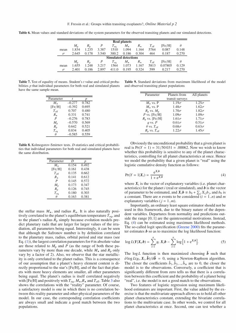
In this section, we detail the statistical method and tests that havebeen used to validate the model. We first perform basic tests ofour model with simulations repeating multiple timesthe numberof observations of the OGLE survey in order to get 50 000 de-tections. This number was chosen as a compromise between sta-tistical significance and computation time. Table 6 compares themean values and standard variations in the observations and inthe simulations. The closeness of the values obtained for the twopopulations is an indication that our approach provides a reason-ably good fit to the real stellar and planetary populations, and tothe real planet compositions and evolution.

However, we do require more advanced statistical tests. First,we use the so-called Student’s t-test to formally compare themean values of all characteristics for both types of planets. Theintuition is that, should the model yield simulated planets of at-tributes similar to real planets, the average values of these at-tributes should not be significantly different from one another.In other words, the so-called null hypothesis H0 is that the dif-ference of their mean is zero. Posing H0: μr − μs = 0 wheresuperscripts r and s denote real and simulated planets respec-tively, and the alternative hypothesis Ha being the complementHa: μr − μs � 0, we compute the t statistics using the first andsecond moments of the distribution of each planet characteristicsas follows:

t =

(μr

x − μsx)

sp√nr+ns

, (2)

where x is each of the planet characteristics, n is the size of eachsample, and sp is the square root of the pooled variance account-ing for the sizes of the two population samples4 The statisticsfollows a t distribution, from which one can easily derive thetwo-tailed critical probability that the two samples come fromone unique population of planets, i.e. H0 cannot be rejected. Theresults are displayed in Table 7 (Note that θ is the Safronov num-ber; other parameters have their usual meaning). In all cases, theprobabilities are greater than 40%, implying that there is no sig-nificant difference in the mean characteristics of both types ofplanets. In other words, the two samples exhibit similar centraltendencies.

Next, we perform the Kolmogorov-Smirnov test to allow fora more global assessment of the compatibility of the two popula-tions. This test has the advantage of being non-parametric, mak-ing no assumption about the distribution of data. This is partic-ularly important since the number of real planets remains small,which may alter the normality of the distribution. Moreover,the Kolmogorov-Smirnov comparison tests the stochastic dom-inance of the entire distribution of real planets over simulatedplanets. To do so, it computes the largest absolute deviations Dbetween Fr(x), the empirical cumulative distribution function ofcharacteristics x for real planets, and Fs(x) the cumulative dis-tribution function of characteristics x for simulated planets, overthe range of values of x: D = max

x{|Freal (x) − Fsim (x)|}. If the

4 The pooled variance is computed as the sum of each sample variancedivided by the overall degree of freedom:

s2p =

∑i,r(xi − μr

x

)2+∑

j,s

(xj − μs

x

)2(nr − 1) + (ns − 1)

(3)

.

calculated D-statistic is greater than the critical D∗-statistic (pro-vided by the Kolmogorov-Smirnov table: for 31 observationsD∗ = 0.19 for a 80% confidence level and D∗ = 0.24 for a 95%confidence level), then one must reject the null hypothesis thatthe two distributions are similar, H0 : |Fr(x) − Fs(x)| < D∗, andaccept Ha : |Fr(x) − Fs(x)| ≥ D∗. Table 8 shows the result of thetest. The first column provides the D-Statistics, and the secondcolumn gives the probability that the two samples have the samedistribution.

Again, we find a good match between the model and ob-served samples: the parameters that have the least satisfactoryfits are the planet’s equilibrium temperature and the planet mass.These values are interpreted as being due to imperfections inthe assumed star and planet populations. It is important to stressthat although the extrasolar planets’ main characteristics (pe-riod, mass) are well-defined by radial-velocity surveys, the sub-set of transiting planets is highly biased towards short periodsand corresponds to a relatively small sample of the known radial-velocity planet population. This explains why the probabilitythat the planetary mass is drawn from the same distribution inthe model and in the observations is relatively low, which mayotherwise seem surprising given that the planet mass distributionwould be expected to be relatively well defined by the radial-velocity measurements.

A.2. Tests in two dimensions

Tests of the adequation of observations and models in twodimensions, i.e. when considering one parameter compared toanother one can be performed using the method of maximumlikelihood as described in Paper I. Table 9 provides values ofthe standard deviations from maximum likelihood for importantcombinations of parameters. The second column is a compari-son using all planets discovered by transit surveys, and the thirdcolumn using all known transiting planets (including those dis-covered by radial velocity).

The results are generally good, with deviations not exceed-ing 1.82σ. They are also very similar when considering all plan-ets or only the subset discovered by photometric surveys. Thisshows that the radial-velocity and photometric planet character-istics are quite similar. The mass vs. radius relation shows thehighest deviation, as a few planets are outliers of our planetaryevolution model.

A.3. Multivariate assessment of the performance of the model

A.3.1. Principle

Tests such as the Student-t statistics and the Kolmogorov-Smirnov test are important to determine the adequacy of givenparameters, but they do not provide a multivariate assessment ofthe model. In order to globally assess the viability of our modelwe proceed as follows: We generate a list including 50 000 “sim-ulated” planets and the 31 “observed” giant planets from Table 1.This number is necessary for an accurate multi-variate analysis(see Sect. A.3.2).A dummy variable Y is generated with value 1if the planet is observed, 0 if the planet is simulated.

In order to test dependencies between parameters, we havepresented in Table 3 (Sect. 2.4) the Pearson correlation coeffi-cients between each variable including Y. A first look at the tableshows that the method correctly retrieves the important physi-cal correlations without any a priori information concerning thelinks that exist between the different parameters. For example,the stellar effective temperature Teff is positively correlated to

F. Fressin et al.: Groups within transiting exoplanets?, Online Material p 2

Table 6. Mean values and standard deviations of the system parameters for the observed transiting planets and our simulated detections.

Real planetsMp Rp P Teq M� R� Teff [Fe/H] θ

mean 1.834 1.235 3.387 1510 1.094 1.164 5764 0.087 0.148σ 2.645 0.178 3.540 300.2 0.186 0.304 464 0.187 0.270

Simulated detectionsMp Rp P Teq M� R� Teff [Fe/H] θ

mean 1.655 1.248 3.217 1564 1.073 1.167 5813 0.07805 0.129σ 2.401 0.186 2.897 411.0 0.195 0.324 599 0.217 0.270

Table 7. Test of equality of means. Student’s t value and critical proba-bilities p that individual parameters for both real and simulated planetshave the same sample mean.

Parameter t pM� –0.277 0.782

[Fe/H] –0.392 0.695Teff 0.707 0.480R� 0.331 0.741P –0.276 0.783

Mp –0.570 0.569Rp 0.642 0.521Teq 0.834 0.405θ –0.585 0.559

Table 8. Kolmogorov-Smirnov tests. D-statistics and critical probabili-ties that individual parameters for both real and simulated planets havethe same distribution.

Parameter D pM� 0.154 0.492

[Fe/H] 0.161 0.438Teff 0.135 0.662R� 0.141 0.612P 0.145 0.572

Mp 0.173 0.347Rp 0.126 0.745Teq 0.180 0.303θ 0.163 0.381

the stellar mass M�, and radius R�. It is also naturally posi-tively correlated to the planet’s equilibrium temperature Teq, andto the planet’s radius Rp simply because evolution models pre-dict planetary radii that are larger for larger values of the irra-diation, all parameters being equal. Interestingly, it can be seenthat although the Safronov number is by definition correlatedto the planetary mass, radius, orbital period and star mass (seeEq. (1)), the largest correlation parameters for θ in absolute valueare those related to Mp and P (as the range of both these pa-rameters vary by more than one decade, while M� and Rp onlyvary by a factor of 2). Also, we observe that the star metallic-ity is only correlated to the planet radius. This is a consequenceof our assumption that a planet’s heavy element content is di-rectly proportional to the star’s [Fe/H], and of the fact that plan-ets with more heavy elements are smaller, all other parametersbeing equal. The planet’s radius is itself correlated negativelywith [Fe/H] and positively with Teq, M�,R� and Teff. Table 3 alsoshows the correlations with the “reality” parameter. Of course,a satisfactory model is one in which there is no correlation be-tween this reality parameter and other physical parameters of themodel. In our case, the corresponding correlation coefficientsare always small and indicate a good match between the twopopulations.

Table 9. Standard deviations from maximum likelihood of the modeland observed transiting planet populations

Parameter Planets from All planetstransit surveys

M� vs. P 1.19σ 1.25σM� vs. P 1.48σ 1.62σRp vs. Mp 1.70σ 1.82σ

P vs. [Fe/H] 1.09σ 1.09σRp vs. [Fe/H] 1.61σ 1.71σg vs. P 0.61σ 0.51σθ vs. Teff 0.68σ 0.63σ

Rp vs. Teff 1.22σ 1.45σ

Obviously the unconditional probability that a given planet isreal is Pr(Y = 1) = 31/50 031 � .00062. Now we wish to knowwhether this probability is sensitive to any of the planet charac-teristics, controlling for all planet characteristics at once. Hencewe model the probability that a given planet is “real” using thelogistic cumulative density function as follows:

Pr(Y = 1|Xi) =eXi b

1 + eXi b(4)

where Xi is the vector of explanatory variables (i.e. planet char-acteristics) for the planet i (real or simulated), and b is the vectorof parameter to be estimated, and Xi b ≡ b0 +

∑j Xi jb j, and b0 is

a constant. There are n events to be considered (i = 1..n) and mexplanatory variables ( j = 1..m).

Importantly, an ordinary least square estimator should not beused in this framework, due to the binary nature of the depen-dent variables. Departures from normality and predictions out-side the range [0; 1] are the quintessential motivations. Instead,Eq. (4) can be estimated using maximum likelihood methods.The so-called logit specification (Greene 2000) fits the parame-ter estimates b so as to maximize the log likelihood function:

log L(Y|X, b) =n∑

i=1

yi Xib −n∑

i=1

log[1 + eXi b

]. (5)

The log L function is then maximized choosing b̂ such that∂ log L(yi, Xi, b̂)/∂b̂ = 0, using a Newton-Raphson algorithm.The closer the coefficients b̂1, b̂2, .., b̂m are to 0, the closer themodel is to the observations. Conversely, a coefficient that issignificantly different from zero tells us that there is a correla-tion between this coefficient and the probability of a planet being“real”, i.e. the model is not a good match to the observations.

Two features of logistic regression using maximum likeli-hood estimators are important. First, the value added by the ex-ercise is that the multivariate approach allows us to hold all otherplanet characteristics constant, extending the bivariate correla-tions to the multivariate case. In other words, we control for allplanet characteristics at once. Second, one can test whether a

F. Fressin et al.: Groups within transiting exoplanets?, Online Material p 3

given parameter estimate is equal to 0 with the usual null hypoth-esis H0: b = 0 versus Ha: b � 0. The variance of the estimator5 isused to derive the standard error of the parameter estimate. UsingEq. (6), dividing each variable b̂ j by the standard error s.e.(b̂ j)yields the t-statistics and allows us to test H0. We note P j theprobability that a higher value of t would occur by chance. Thisprobability is evaluated for each explanatory variable j. Shouldour model perform well, we would expect the t value of each pa-rameter estimate to be null, and the corresponding probabilityP jto be close to one. This would imply no significant associationbetween a single planet characteristics and the event of being a“real” planet.

The global probability that the model and observations arecompatible can be estimated. To do so, we compute the log like-lihood obtained when b j = 0 for j = 1..m, where m is the numberof variables. Following Eq. (6):

log L(Y|1, b0) =n∑

i=1

yib0 −n∑

i=1

log[1 + eb0

]. (6)

The maximum of this quantity is log L0 = n0 log(n0/n) +n1 log(n1/n), where n0 is the number of cases in which y = 0and n1 is the number of observations with y = 1. L0 is thus themaximum likelihood obtained for a model which is in perfectagreement with the observations (no explanatory variable is cor-related to the probability of being real). Now, it can be shownthat the likelihood statistic ratio

cLL = 2(log L1 − log L0) (7)

follows a χ2 distribution for a number of degrees of freedomm when the null hypothesis is true (Aldrich & Nelson 1984).The probability that a sum of m normally distributed randomvariables with mean 0 and variance 1 is larger than a value cLL is:

Pχ2 = P(m/2, cLL/2), (8)

where P(k, z) is the regularized Gamma function (e.g.Abramowitz & Stegun (1964)). Pχ2 is thus the probability thatthe model planets and the observed planets are drawn from thesame distribution.

A.3.2. Determination of the number of model planets required

A problem that arose in the course of the present work was toevaluate the number of model planets that were needed for thelogit evaluation. It is often estimated that about 10 times moremodel points than observations are sufficient for a good tests. Wefound that this relatively small number of points indeed leads to avalid identification of the explanatory variables that are problem-atic, i.e. those for which the b̂ coefficient is significantly differentfrom 0 (if any). However, the evaluation of the global χ2 proba-bility was then found to show considerable statistical variability,probably given the relatively large number of explanatory vari-ables used for the study.

In order to test how the probability Pχ2 depends on the sizen of the sample to be analyzed, we first generated a very largelist of N0 simulated planets with CoRoTlux. We generated withMonte-Carlo simulations a smaller subset of n0 ≤ N0 simulatedplanets that was augmented by the n1 = 31 observed planetsand computed Pχ2 using the logit procedure. This exercise wasperformed 1000 times, and the results are shown in Fig. 13. The

5 The variance of the estimator is provided by the Hessian∂2 log L(yi|Xi, b)/∂b∂b′.

.5.6

.7.8

.9P

rob

> C

hi−

Squ

are

0 10000 20000 30000 40000 50000Sample Size

Fig. 13. Values of the χ2 probability, Pχ2 (see text) obtained after a logitanalysis as a function of the size of the sample of model planets n0.

resulting Pχ2 is found to be very variable for a sample smallerthan ∼20 000 planets. As a consequence, we chose to presenttests performed for n0 = 50 000 model planets.

A.3.3. Analysis of two CoRoTlux samples

Table 4 (see Sect. 2.4) reports the parameter estimates for eachof the planet/star characteristics. We start by assessing the gen-eral quality of the logistic regression by performing the chi-square test. If the vector of planet characteristics brings no orlittle information as to which type of planets a given observa-tion belongs, we would expect the logistic regression to performbadly. In technical terms, we would expect the conditional prob-ability Pr(Y = 1|X) to be equal to the unconditional probabilityPr(Y = 1). The χ2 test described above is used to evaluate thesignificance of the model.

We performed several tests: the first column of results inTable 10 shows the result of a logit analysis with the whole seriesof 9 explanatory variables. Globally, the model behaves well,with a likelihood statistic ratio cLL = 5.8 and a χ2 distributionfor 9 degrees of freedom yielding a probability Pχ2 = 0.758.When examining individual variables, we find that the low-est probability derived from the Student test is that of [Fe/H]:P[Fe/H] = 0.164, implying that the stellar metallicity is not wellreproduced. As discussed previously, this is due to the fact thatseveral planets of the observed list have no or very poorly con-strained determinations of the stellar [Fe/H], and so a defaultvalue of 0 was then used.

The other columns in Table 10 show the result of the logitanalysis when removing one variable (i.e. with only 8 explana-tory variables). In agreement with the above analysis, the high-est global probability Pχ2 is obtained for the model without the[Fe/H] variable. When removing other variables, the results arevery homogeneous, indicating that although the model can cer-tainly be improved, there is no readily identified problem exceptthat for [Fe/H]. We hope that future observations will allow forbetter constraints on these stars’ metallicities.

In order to further test the method, we show in Table 11 theresults of an analysis in which the model radii where artificiallyaugmented by 10%. The corresponding probabilities are signifi-cantly lower: we find that the model can explain the observationsby chance only in less than 1/10 000. The probabilities for eachvariable are affected as well so that it is impossible to identifythe culprit for the bad fit with the 9 variables. However, whenremoving Rp from the analysis sample, the fit becomes signif-icantly better. Note that the results for that column are slightlydifferent of those for the same column in Table 10 because of thedependance of θ on Rp.

F. Fressin et al.: Groups within transiting exoplanets?, Online Material p 4

Table 10. Results of the logit analysis for the fiducial model with 50 000 model planets and 31 observations.

All variables Missing variable[Fe/H] Teff R� M� P Rp Mp θ Teq

[Fe/H] b̂[Fe/H] 0.415 0.435 0.413 0.430 0.421 0.229 0.385 0.371 0.369P[Fe/H] [0.164] [0.148] [0.164] [0.150] [0.157] [0.242] [0.177] [0.196] [0.182]

Teff b̂Teff –0.517 –0.579 –0.541 –0.191 –0.569 –0.563 –0.541 –0.537 –0.618PTeff [0.417] [0.366] [0.372] [0.601] [0.355] [0.378] [0.391] [0.395] [0.298]

R� b̂R� 0.059 0.046 0.190 0.212 –0.009 0.061 0.027 0.023 –0.063PR� [0.901] [0.924] [0.681] [0.609] [0.984] [0.898] [0.953] [0.961] [0.871]

M� b̂M� 0.467 0.541 –0.001 0.511 0.472 0.524 0.483 0.486 0.497PM� [0.528] [0.468] [0.998] [0.433] [0.523] [0.481] [0.512] [0.508] [0.499]

P b̂P –0.236 –0.288 –0.425 –0.199 –0.250 –0.281 –0.269 –0.356 –0.070PP [0.746] [0.698] [0.605] [0.754] [0.737] [0.706] [0.708] [0.618] [0.883]

Rp b̂Rp 0.305 –0.069 0.331 0.305 0.328 0.316 0.261 0.246 0.241PRp [0.370] [0.778] [0.332] [0.370] [0.336] [0.352] [0.416] [0.456] [0.443]

Mp b̂Mp 0.329 –0.032 0.432 0.306 0.379 0.386 0.055 –0.229 0.118PMp [0.726] [0.968] [0.656] [0.737] [0.693] [0.674] [0.947] [0.474] [0.876]

θ b̂θ –0.904 –0.496 –1.005 –0.879 –0.971 –1.049 –0.625 –0.422 –0.653Pθ [0.563] [0.706] [0.540] [0.567] [0.548] [0.497] [0.658] [0.410] [0.620]

Teq b̂Teq –0.296 –0.023 –0.520 –0.250 –0.339 –0.169 –0.089 –0.186 –0.150PTeq [0.648] [0.970] [0.414] [0.635] [0.605] [0.744] [0.882] [0.742] [0.801]

overall assessment of the fitLog likelihood –257.059 –258.123 –257.410 –257.066 –257.275 –257.129 –257.439 –257.126 –257.316 –257.171

cLL 5.821 3.692 5.119 5.805 5.389 5.681 5.060 5.687 5.307 5.597Pχ2 0.758 0.884 0.745 0.669 0.715 0.683 0.751 0.682 0.724 0.692

Table 11. Results of the logit analysis for the altered model (Rp increased by 10%) with 50 000 model planets and 31 observations.

All variables Missing variable[Fe/H] Teff R� M� P Rp Mp θ Teq

[Fe/H] b̂[Fe/H] –0.738 –0.740 –0.737 –0.737 –0.733 0.224 –0.607 –0.728 –0.664P[Fe/H] [0.002] [0.002] [0.002] [0.002] [0.002] [0.251] [0.009] [0.002] [0.005]

Teff b̂Teff –0.729 –0.713 –0.742 –0.255 –0.819 –0.573 –0.545 –0.739 –0.308PTeff [0.260] [0.268] [0.231] [0.483] [0.192] [0.366] [0.404] [0.256] [0.618]

R� b̂R� 0.032 0.013 0.197 0.247 –0.091 0.032 0.237 0.018 0.558PR� [0.945] [0.978] [0.661] [0.540] [0.828] [0.945] [0.620] [0.970] [0.149]

M� b̂M� 0.677 0.650 0.017 0.702 0.684 0.532 0.557 0.667 0.598PM� [0.370] [0.388] [0.966] [0.291] [0.363] [0.472] [0.461] [0.377] [0.430]

P b̂P –0.417 –0.356 –0.664 –0.395 –0.432 –0.366 –0.393 –0.249 –1.706PP [0.585] [0.618] [0.421] [0.565] [0.575] [0.622] [0.641] [0.716] [0.037]

Rp b̂Rp –1.986 –1.264 –1.974 –1.986 –1.985 –1.995 –1.763 –1.973 –1.796PRp [0.000] [0.000] [0.000] [0.000] [0.000] [0.000] [0.000] [0.000] [0.000]

Mp b̂Mp –1.359 –0.894 –1.350 –1.359 –1.354 –1.305 –0.328 –1.150 –1.045PMp [0.001] [0.019] [0.002] [0.001] [0.001] [0.001] [0.558] [0.001] [0.052]

θ b̂θ 0.384 0.271 0.461 0.376 0.387 0.193 0.021 –1.714 0.338Pθ [0.359] [0.541] [0.327] [0.347] [0.372] [0.494] [0.976] [0.009] [0.633]

Teq b̂Teq 1.189 0.797 0.940 1.212 1.165 1.439 –0.009 0.603 1.202PTeq [0.045] [0.162] [0.100] [0.014] [0.051] [0.001] [0.987] [0.334] [0.054]

overall assessment of the fitLog likelihood –243.645 –247.922 –244.341 –243.648 –244.098 –243.872 –257.580 –246.194 –243.872 –245.271

cLL 32.647 24.094 31.256 32.643 31.743 32.194 4.778 27.551 32.194 29.395Pχ2 0.000 0.002 0.000 0.000 0.000 0.000 0.781 0.001 0.000 0.000