Tidal stream device reliability comparison models Tidal stream device reliability comparison models
Upload
khangminh22Category
view
3download
0
TIDAL INTERACTIONS OF SHORT-PERIOD
EXTRASOLAR TRANSIT PLANETS WITH THEIR HOST
STARS: CONSTRAINING THE ELUSIVE STELLAR
TIDAL DISSIPATION FACTOR
Inaugural-Dissertation
zur
Erlangung des Doktorgrades
der Mathematisch-Naturwissenschaftlichen Fakultat
der Universitat zu Koln
vorgelegt von
Ludmila Carone
aus Bukarest

Berichterstatter: PD. Dr. M. Patzold
Prof. Dr. L. Labadie
Prof. Dr. H. Rauer
Tag der mundlichen Prufung: 22.5.2012

Abstract
The orbital and stellar rotation evolution of CoRoT planetary systems due to tides
raised by the planet on the star (stellar tidal friction) and by tides raised by the
star on the planet (planetary tidal friction, for e > 0) is investigated. The evolution
time scale depends on the stellar tidal dissipation factor over stellar Love number
Q∗/k2,∗ which is not very well constrained. Tidal energy dissipation models yield
Q∗/k2,∗ = 105 − 109.
Many CoRoT planets may migrate towards their star because the stellar rotation
rate Ω∗ is smaller than the planetary mean revolution rate n. To guarantee long-term
stability of the CoRoT-planets, Q∗k2,∗
≥ 107−108 is derived as a common stability limit.
As the planet migrates towards the star, the stellar rotation is spun-up efficiently. For
most CoRoT stars no sign of tidal spin up is found, therefore Q∗k2,∗
> 106 is derived by
requiring tidal friction to be weaker than magnetic braking. CoRoT-17 apparently is
experiencing moderate tidal spin-up which requires 4× 10⁷ ≤ Q∗k2,∗
< 109.
For planets with e ≥ 0.5, like CoRoT-10b and CoRoT-20b, planetary and stellar
tidal friction may act on similar timescales. This may lead to a positive feedback
effect, decreasing the semi major axis/increasing the stellar rotation rapidly. To
avoid this, Q∗k2,∗
> 106 is required.
The CoRoT-3 and CoRoT-15 system may be tidal equilibrium states, where Ω∗ =
n. To achieve this state and to maintain it in the presence of magnetic brakingQ∗k2,∗
≤ 107 − 108 is required. Even then, the double synchronous orbit may decay
because magnetic braking removes angular momentum from the system. Therefore,
only F stars are capable to maintain a double synchronous state with a massive
companion, because these stars are not strongly affected by magnetic braking.
The Q∗k2,∗
values required for double synchronous rotation are comparatively low
although Q∗k2,∗
is expected to grow as Ω∗ → n. This discrepancy is explained by the
on-set of dynamical tides as stellar eigenfrequencies are exited, leading to a more
efficient tidal energy dissipation and reducing Q∗k2,∗
. The other CoRoT-systems are
assumed not to excite dynamical tides.
i

Kurzzusammenfassung
Die Entwicklung des Orbits und der Sternrotation von CoRoT Planetensyste-
men aufgrund von stellarer Gezeitenreibung und planetarer Gezeitenreibung wird
untersucht. Die Entwicklungszeitraume hangen vom stellaren Gezeitendissipations-
factor uber stellare Love-Zahl Q∗/k2,∗ ab, deren Grosse nicht genau bekannt ist. Aus
Gezeitenenergie-Dissipations-Modelle ergeben sich: Q∗/k2,∗ = 105 − 109.
Viele CoRoT-Planeten konnten zum Stern wandern, da Ω∗ < n. Um das Uberleben
der CoRoT-Planeten zu garantieren, ergibt sich Q∗k2,∗
≥ 107 − 108 als Stabilitatslimit.
Wenn der Planet zum Stern wandert, wird die Sternrotation stark beschleunigt.
Die meisten CoRoT-Sterne zeigen kein Zeichen einer Gezeitenbeschleunigung, daher
ergibt sich Q∗k2,∗
> 106, wenn angenommen wird, dass Gezeitenreibung schwacher ist
als ’magnetic braking’. Die Rotation von CoRoT-17 scheint moderat durch Gezeit-
enreibung beschleunigt zu werden, woraus sich 4× 10⁷ ≤ Q∗k2,∗
< 109 ergibt.
Planeten mit e ≥ 0.5, wie CoRoT-10b und CoRoT-20b, sind gleichzeitig planetarer
und stellarer Gezeitenreibung unterworfen. Das fuhrt zu einer positiven Ruckkopplung,
wobei sich die große Halbachse stark verringert bzw. die Sternrotation stark beschle-
unigt. Um dies zu verhindern, ist Q∗k2,∗
> 106 erforderlich.
Das CoRoT-3 and CoRoT-15-System konnte in einem Gleichgewichtszustand sein,
so dass Ω∗ = n. Um diesen Zustand trotz ’magnetic braking’ aufrechtzuerhalten,
ist Q∗k2,∗
≤ 107 − 108 erforderlich. Selbst dann konnte der doppelt-synchrone Orbit
aufgrund von ’magnetic braking’ zerfallen. Daher konnen nur F-Sterne einen doppelt-
synchronen Zustand mit einem schweren Begleiter aufrechterhalten, weil diese Sterne
reduziertem ’magnetic braking’ unterworfen sind.
Die Q∗k2,∗
-Werte fur den doppelt-synchronen Zustand sind verhaltnismassig klein,
obwohl erwartet wird, dass Q∗k2,∗
wachst, wenn Ω∗ → n. Das kann durch dynamische
Gezeiten erklart werden, wenn stellare Eigenfrequenzen angeregt werden. Das fuhrt
zu einer effizienten Gezeitenenergie-Dissipation und einem kleineren Q∗k2,∗
. Es wird
angenommen, dass die anderen CoRoT-Systeme keine dynamischen Gezeiten anregen.
ii

Table of Contents
Table of Contents iii
List of Tables vii
List of Figures ix
Variables and constants 1
Introduction 4
1 Extrasolar planets and Brown Dwarfs 10
1.1 Definition of extrasolar planets
and brown dwarfs . . . . . . . . . . . . . . . . . . . . . . . . . . . . . 10
1.2 History of extrasolar planet detection . . . . . . . . . . . . . . . . . . 13
1.3 Extrasolar planets detection methods . . . . . . . . . . . . . . . . . . 15
1.3.1 Indirect detection methods . . . . . . . . . . . . . . . . . . . . 15
1.3.2 Direct detection methods . . . . . . . . . . . . . . . . . . . . . 24
1.4 CoRoT . . . . . . . . . . . . . . . . . . . . . . . . . . . . . . . . . . . 31
1.5 Overview of exoplanet properties . . . . . . . . . . . . . . . . . . . . 37
2 Theory of tidal interaction 41
2.1 The gravitational potential . . . . . . . . . . . . . . . . . . . . . . . . 42
2.1.1 The outer gravitational potential . . . . . . . . . . . . . . . . 42
2.1.2 Inner gravity potential . . . . . . . . . . . . . . . . . . . . . . 45
2.2 The role of Legendre polynomials in axial symmetric gravity potentials 46
2.2.1 Potential theory . . . . . . . . . . . . . . . . . . . . . . . . . . 48
2.3 Tidal force and potential . . . . . . . . . . . . . . . . . . . . . . . . . 51
2.4 Deformation of celestial bodies . . . . . . . . . . . . . . . . . . . . . . 57
2.4.1 Tidal deformation . . . . . . . . . . . . . . . . . . . . . . . . . 57
iii

2.4.2 Rotational Deformation . . . . . . . . . . . . . . . . . . . . . 64
2.5 Tidal waves in the forced damped oscillator framework . . . . . . . . 70
2.6 Tidal torques . . . . . . . . . . . . . . . . . . . . . . . . . . . . . . . 73
2.7 Tidal evolution of eccentric orbits . . . . . . . . . . . . . . . . . . . . 80
2.8 The tidal dissipation factor and the Love number . . . . . . . . . . . 89
2.8.1 Q/k2 in the Solar System . . . . . . . . . . . . . . . . . . . . 90
2.8.2 Q/k2 in extrasolar planet systems . . . . . . . . . . . . . . . . 94
2.9 Stability of tidal equilibrium . . . . . . . . . . . . . . . . . . . . . . . 98
2.10 Evolution of the rotation of main sequence stars . . . . . . . . . . . . 105
2.11 Moment of Inertia . . . . . . . . . . . . . . . . . . . . . . . . . . . . . 113
2.12 The Roche limit . . . . . . . . . . . . . . . . . . . . . . . . . . . . . . 115
3 Critical examination of assumptions and approximations 119
3.1 The constant Q∗-assumption . . . . . . . . . . . . . . . . . . . . . . . 119
3.1.1 Can Q∗ be regarded as constant even though the system may
meet resonant states? . . . . . . . . . . . . . . . . . . . . . . . 120
3.1.2 Can Q∗ be regarded as constant although it is defined as fre-
quency dependent? . . . . . . . . . . . . . . . . . . . . . . . . 121
3.1.3 What happens with Q∗ when the system approaches double
synchronicity? . . . . . . . . . . . . . . . . . . . . . . . . . . . 122
3.1.4 Switching from the constant Q- to the constant τ -formalism. . 124
3.2 Is the planetary rotation tidally locked? . . . . . . . . . . . . . . . . . 126
3.3 Energy and angular momentum in close-in extrasolar planetary systems131
3.3.1 Possible pitfalls in the calculation of the Roche zone . . . . . . 133
4 Close-in extrasolar planets as playground for tidal friction models 136
4.1 The tidal stability maps for planets around main sequence stars . . . 136
4.1.1 CoRoT systems most strongly affected by tidal friction . . . . 144
5 Constraining Q∗k2,∗
by requiring orbital stability of close-in planets
around slowly rotating stars 149
5.1 Tidal evolution of the semi major axis of CoRoT-Planets on circular
orbits . . . . . . . . . . . . . . . . . . . . . . . . . . . . . . . . . . . . 150
5.1.1 Tidal evolution of the semi major axis of CoRoT-Planets on
circular orbits around low mass stars . . . . . . . . . . . . . . 151
5.1.2 Tidal evolution of the semi major axis of planets on circular
orbits around F stars and subgiants . . . . . . . . . . . . . . . 156
5.2 Tidal evolution of the semi major axis and eccentricity of planets on
eccentric orbits . . . . . . . . . . . . . . . . . . . . . . . . . . . . . . 158
iv
5.2.1 How does the semi major axis and eccentricity evolution change
with larger QPl
k2,P l. . . . . . . . . . . . . . . . . . . . . . . . . . 167
5.2.2 Positive feedback effect for planets on orbits with
e > 0.5 . . . . . . . . . . . . . . . . . . . . . . . . . . . . . . . 174
5.2.3 Orbital stability for planets on eccentric orbits . . . . . . . . . 175
5.3 Limits of stability on potentially unstable systems . . . . . . . . . . . 177
6 Constraining Q∗k2,∗
by stellar rotation evolution of slowly rotating stars178
6.1 Tidal rotation evolution of the host stars of CoRoT-Planets on circular
orbits . . . . . . . . . . . . . . . . . . . . . . . . . . . . . . . . . . . . 179
6.1.1 Tidal rotation evolution of low mass host stars of CoRoT-Planets
on circular orbits . . . . . . . . . . . . . . . . . . . . . . . . . 180
6.1.2 Tidal rotation evolution of F-spectral type host stars of CoRoT-
Planets on circular orbits . . . . . . . . . . . . . . . . . . . . . 183
6.2 Tidal rotation evolution of host stars of CoRoT-Planets on eccentric
orbits . . . . . . . . . . . . . . . . . . . . . . . . . . . . . . . . . . . . 190
6.2.1 How does the stellar rotation evolution change with larger QPl
k2,P l194
6.2.2 Positive feedback effect for planets on orbits with
e > 0.5 . . . . . . . . . . . . . . . . . . . . . . . . . . . . . . . 194
6.3 Using stellar rotation as a ’smoking gun’ for the influence of tidal friction198
6.4 Evaluating evidence for tidal spin up . . . . . . . . . . . . . . . . . . 203
6.5 A word regarding the evolution of the tidal frequencies . . . . . . . . 204
7 Tidal evolution of close-in exoplanets around fast rotating stars 205
7.1 The tidal evolution of the CoRoT-6 system . . . . . . . . . . . . . . . 210
7.2 The tidal evolution of the CoRoT-11 system . . . . . . . . . . . . . . 212
7.3 Orbital stability . . . . . . . . . . . . . . . . . . . . . . . . . . . . . . 216
7.4 Results of the stellar rotation evolution . . . . . . . . . . . . . . . . . 216
8 Double synchronous states 219
8.1 The stability of the double synchronous CoRoT systems . . . . . . . 219
8.2 Constraints on Q∗k2,∗
to achieve a double synchronous state in the pres-
ence of magnetic braking . . . . . . . . . . . . . . . . . . . . . . . . . 224
8.3 Long-term stability of double synchronous orbits in the presence of
magnetic braking . . . . . . . . . . . . . . . . . . . . . . . . . . . . . 233
8.3.1 The possible decay of the double synchronous orbit due to mag-
netic braking . . . . . . . . . . . . . . . . . . . . . . . . . . . 236
8.4 Tidal evolution of the CoRoT-3 and CoRoT-15 system . . . . . . . . 240
v

8.4.1 Why will CoRoT-20 not be able to maintain a stable double
synchronous state? . . . . . . . . . . . . . . . . . . . . . . . . 249
8.4.2 Limits on Q∗k2,∗
to currently maintain a double synchronous ro-
tation state . . . . . . . . . . . . . . . . . . . . . . . . . . . . 259
9 Summary and Discussion 263
Appendix 273
A CoRoT planet references 274
B Tidal evolution of CoRoT-4 and CoRoT-9 276
C |Ω∗ − n| evolution for close-in CoRoT-planets 279
D Evolution of the rotation of CoRoT planets on eccentric orbits 289
E Integration method 293
F Model sensitivity analysis 299
F.1 The CoRoT-12 system . . . . . . . . . . . . . . . . . . . . . . . . . . 300
F.2 The CoRoT-16 system . . . . . . . . . . . . . . . . . . . . . . . . . . 302
F.3 The CoRoT-20 system . . . . . . . . . . . . . . . . . . . . . . . . . . 304
F.4 The CoRoT-11 system . . . . . . . . . . . . . . . . . . . . . . . . . . 308
F.5 The CoRoT-15 system . . . . . . . . . . . . . . . . . . . . . . . . . . 308
G Proof that the double synchronous orbit is always forced into cor-
rotation if Lorb > Lorb,crit 313
H Centrifugal versus gravitational force 315
Acknowledgements 339
Erklarung 340
Lebenslauf 341
vi

List of Tables
1.1 Planet types discovered by the CoRoT space mission. . . . . . . . . . 32
1.2 Stellar parameters of CoRoT-1 to -21. . . . . . . . . . . . . . . . . . . 34
1.3 Planetary parameters of CoRoT-1b to -21b. . . . . . . . . . . . . . . 35
1.4 Stellar rotation period of CoRoT-1 to -21 and planetary revolution of
CoRoT-1b to -21b. . . . . . . . . . . . . . . . . . . . . . . . . . . . . 36
2.1 Normalized moment of inertia for some ideal bodies . . . . . . . . . . 114
2.2 Normalized moment of inertia for some solar system bodies . . . . . . 114
3.1 Synchronization time scale τsynchr for the CoRoT-planets. A slow ro-
tator is a planet with an initial rotation period PPl = 10 days, a fast
rotator is a planet with an initial rotation period of PPl = 10 hours. . 128
3.2 Comparison of Roche limit approximations . . . . . . . . . . . . . . . 135
4.1 The parameters of the central stars used for the calculation of the tidal
stability maps. Real stars were selected as representatives of K-, G-
and F-spectral type stars, respectively. . . . . . . . . . . . . . . . . . 138
4.2 The parameters of the exoplanets placed around each star (Table 4.1)
for the calculation of the tidal stability map. A real planet was selected
as a representative for each exoplanet category. . . . . . . . . . . . . 139
5.1 Required Q∗k2,∗ stable
for the planet’s orbit to stay outside the Roche limit
within the minimum, average, and maximum remaining lifetime of the
star. . . . . . . . . . . . . . . . . . . . . . . . . . . . . . . . . . . . . 155
vii

5.2 Required Q∗k2,∗ stable
(eq. 5.1.2) for the planet’s orbit to stay outside the
Roche limit within the remaining lifetime of the star. . . . . . . . . . 157
5.3 Equivalent semi major axis aequiv (equation 5.2.8) of the CoRoT-planets
on eccentric orbits. . . . . . . . . . . . . . . . . . . . . . . . . . . . . 173
5.4 Required Q∗k2,∗ stable
for the planet’s orbit to stay outside the Roche limit
within the minimum, average and maximum remaining lifetime of the
star. . . . . . . . . . . . . . . . . . . . . . . . . . . . . . . . . . . . . 176
6.1 Required Q∗k2,∗
for tidal friction to compensate magnetic braking at the
planet’s current position. . . . . . . . . . . . . . . . . . . . . . . . . . 199
6.2 Required Q∗k2,∗
for tidal friction to compensate magnetic braking for
planets on eccentric orbits at the current position. . . . . . . . . . . . 202
7.1 Required Q∗k2,∗ stable
for the planet’s orbit to stay outside the Roche limit
within the remaining lifetime of the star. . . . . . . . . . . . . . . . . 217
8.1 Required Q∗k2,∗
for tidal friction to compensate magnetic braking at the
planet’s current position. . . . . . . . . . . . . . . . . . . . . . . . . . 259
8.2 Required Q∗k2,∗
for tidal friction to allow for minimal migration in the past.261
A.1 References for the parameters of the CoRoT planetary systems. . . . 275
viii

List of Figures
1.1 Histogram of the masses of all detected exoplanets. The data were
taken from the exoplanet catalogue: http://www.exoplanet.eu/catalog-
all.php as of 14th October 2011. . . . . . . . . . . . . . . . . . . . . 12
1.2 The motion of a star and a planet with masses M∗ and MPl and semi
major axes a∗ and aPl, respectively, around their common center of
mass (CM). . . . . . . . . . . . . . . . . . . . . . . . . . . . . . . . . 16
1.3 The orbital plane of a planetary system which is inclined by the angle
i with respect to the line-of-sight. The system consists of a star and
a planet with masses M∗ and MPl, revolving with semi major axes a∗
and aPl, respectively, around their common center of mass. . . . . . . 17
1.4 As the star moves around the barycenter, emitted light is Doppler
shifted (Credit: ESO). . . . . . . . . . . . . . . . . . . . . . . . . . . 19
1.5 Radial velocity curve of 51 Pegasi b. The planet induces a radial
velocity modulation of about 50 m/s (Mayor and Queloz, 1995). . . . 21
1.6 Left panel: Schema of the microlensing effect (Credit: OGLE).
Right panel: Photometric curve with best-fitting double-lens models
of OGLE 2003-BLG-235/MOA 2003-BLG-53 b (Bond et al., 2004). . 25
1.7 Composite image of the brown dwarf 2M1207 and its gas giant com-
panion in the infrared (Chauvin et al., 2004). . . . . . . . . . . . . . . 27
1.8 As the planet passes in front of its star, the apparent brightness of the
star decreases by ∆F (Credit: Hans Deeg, ESA). . . . . . . . . . . . 28
1.9 Probability to observe a transit from Earth. . . . . . . . . . . . . . . 29
ix

1.10 Artistic view of the satellite CoRoT in polar orbit around Earth (CNES,
D.Ducros). . . . . . . . . . . . . . . . . . . . . . . . . . . . . . . . . . 31
1.11 The CoRoT ’eyes’ in the night sky (diameter:10). The ’red’ circle is
observed in summer and contains the Aquila constellation. The ’blue’
circle is observed in winter and lies in the Monoceros constellation
(CNES). . . . . . . . . . . . . . . . . . . . . . . . . . . . . . . . . . . 32
1.12 Histogram of the masses of all detected exoplanets in logarithmic scale. 37
1.13 Left panel: Histogram of the semi major axis of all detected exoplanets.
Right panel: Histogram of the semi major axis of exoplanets in close
proximity to their star in units of solar radii. . . . . . . . . . . . . . . 38
1.14 Left panel: Histogram of the masses of all detected transiting exoplan-
ets. Right panel: Histogram of the masses of all detected transiting
exoplanets in logarithmic scale. . . . . . . . . . . . . . . . . . . . . . 39
1.15 Left panel: Histogram of the semi major axis of all detected transiting
exoplanets. Right panel: Histogram of the semi major axis of transiting
exoplanets in units of solar radii. . . . . . . . . . . . . . . . . . . . . 40
2.1 The parameters of the mass element dm in polar coordinates. . . . . 43
2.2 The distance ∆ between P , the position of the mass element dm, and
the reference point P ′ in polar coordinates . . . . . . . . . . . . . . . 44
2.3 The potential of mass element at Pi as seen from an outer reference
point P ′ in a spherical coordinate system. . . . . . . . . . . . . . . . 47
2.4 The location of two points P and P ′ on a unit sphere. . . . . . . . . . 50
2.5 The relationships between the radius of the primary, RP , the radius of
the orbit of the secondary, a, and the distance ∆ from a point P on
the surface of the primary to the center of mass of the secondary. . . 52
2.6 Centrifugal versus gravitational force at different points within the pri-
mary. . . . . . . . . . . . . . . . . . . . . . . . . . . . . . . . . . . . . 54
x

2.7 The particles in a primary move on circles of identical radii aP , which is
the distance from the primary’s center of mass to the common center of
gravity CM . This is illustrated by the movement of P ′ about the point
CM ′ and the center of the primary CP about CM . In this picture the
rotation of the primary about its polar axis is neglected. . . . . . . . 55
2.8 The deformation of a homogenous sphere due to the tidal potential. . 58
2.9 The tidal deformation of a two-component model planet of radius
Rmean and density ρo and a core of radius RCore and density ρc. . . . 61
2.10 Centrifugal force in a primary rotating about its polar axis with the
rotation rate Ω in a coordinate system where the angle θ is measured
from the rotation axis. . . . . . . . . . . . . . . . . . . . . . . . . . . 65
2.11 Left: Symmetry axis with respect to the tidal deformation.
Right: Symmetry axis with respect to the rotation of the body. . . . 69
2.12 Upper panel: If the primary’s rotation is faster than the secondary’s
revolution (ΩP > n), the tidal bulge is carried ahead the line con-
necting the two center of masses. The tidal torques decrease ΩP and
increase n.
Middle panel: If the primary’s rotation is slower than the secondary’s
revolution (ΩP < n), the tidal bulge is lagging behind the line con-
necting the two center of masses. The tidal torques increase ΩP and
decrease n.
Lower panel: If the system is in retrograde revolution, the tidal torques
decrease ΩP and n. . . . . . . . . . . . . . . . . . . . . . . . . . . . 77
2.13 The barycentric orbit configuration of a binary system including its
relevant parameters. L is the total angular momentum Ltot and h is
the orbital angular momentum Lorb (Hut, 1980). . . . . . . . . . . . . 99
xi

2.14 Total angular momentum of a binary system in double synchronous
rotation Ltot,doub versus orbital revolution rate n (Hut, 1980). For n >
ncrit, two double synchronous states exist. Arrows show the direction
of decreasing total energy. The stability of a given double synchronous
state is determined by the total energy: Stability is only ensured if the
total energy is minimal as well. For n = ncrit only one solution with
Ltot,doub = Lcrit exists. For Ltot,doub < Lcrit, no double synchronous
state can be achieved. . . . . . . . . . . . . . . . . . . . . . . . . . . 104
2.15 Evolution of the stellar radius, radius of gyration I (=moment of inertia
C∗ in the notation used in this work) for 0.5, 0.8 and 1MSun stars
(Bouvier et al., 1997). . . . . . . . . . . . . . . . . . . . . . . . . . . 106
2.16 Ca+ emission luminosity, rotation velocity and lithium abundance with
age. Shown as an example are the properties of stars in the Pleidaes
(0.04 Gyrs), Ursa Major (0.15 Gyrs), the Hyades Cluster (0.4 Gyrs)
and the Sun (4.5 Gyrs). In 1972 the age estimate of the Hyades Cluster
was controversial. Other age estimates would have resulted in a shift
of the Pleiades data points along the x-axis as indicated by the arrows
(Skumanich, 1972). . . . . . . . . . . . . . . . . . . . . . . . . . . . . 109
2.17 Color-period diagrams (B−V versus rotation period, on a linear scale)
for a series of open clusters and Mount Wilson stars with different ages.
Note the change in scale for the old Mount Wilson stars. The higher
B−V , the redder the star, the less hot the stellar surface and the lower
the mass of the star. On the other hand, the smaller B − V , the bluer
the star, the hotter the stellar surface, the higher the mass of the star
(Barnes, 2003). . . . . . . . . . . . . . . . . . . . . . . . . . . . . . . 112
2.18 The solar seismic model taken from Dziembowski et al. (1994). r is the
radius from the center of the Sun, u is the square of isothermal speed
of sound at radius r, ρ is the density at radius r, P is the pressure and
M(r) is the integrated mass up to r. . . . . . . . . . . . . . . . . . . 115
xii

3.1 Left panel: Planetary revolution period versus semi major axis of a
close-in extrasolar Jupiter analogue around a Sun-like star.
Right panel: Planetary revolution rate versus semi major axis of a
close-in extrasolar Jupiter analogue around a Sun-like star. . . . . . . 121
3.2 Synchronization time scales τsynchr and the age of the CoRoT planets
versus their semi major axes. The black solid lines represent τsynchr
calculated for a slow (10 days) and a fast (10 hours) primordial plan-
etary rotation. The grey lines represent the system ages within the
limit of uncertainties. The age of CoRoT-9b, a planet orbiting its star
beyond 0.4 AU, is represented by a dotted grey line. In this case, the
system age and the possible synchronization time scale overlap each
other. . . . . . . . . . . . . . . . . . . . . . . . . . . . . . . . . . . . 129
3.3 Relative brightness in the infrared estimated for 12 longitudinal strips
on the surface of the planet HD 189733. Data are shown as a colour
map (a) and in graphical form (b) (Knutson et al., 2007). . . . . . . . 130
3.4 Density of transiting exoplanets versus their mass. . . . . . . . . . . . 134
4.1 Tidal stability maps for different exoplanets around a K-star. From
top to bottom, from left to right: A high mass brown dwarf, a low
mass brown dwarf, a hot Jupiter, a Neptune, a Super-Earth, an Earth
and a Mercury planet. The grey color gives the time scale τRoche in
log(109 years). The total lifetime of the star is indicated as a white
dashed line. The black lines are the isochrones of τRoche. The horizontal
and vertical dashed white lines indicate the stability limit athreshold for
every Q∗k2,∗
. . . . . . . . . . . . . . . . . . . . . . . . . . . . . . . . . . 141
4.2 Tidal stability maps for different exoplanets around a G-star. See also
Figure 4.1. . . . . . . . . . . . . . . . . . . . . . . . . . . . . . . . . . 142
4.3 Tidal stability maps for different exoplanets around an F-star. See also
Figure 4.1. . . . . . . . . . . . . . . . . . . . . . . . . . . . . . . . . . 143
xiii

4.4 Doodson constants for tides raised on the star by CoRoT-1 to CoRoT-
21b and several Solar System bodies. M marks the Doodson constant
for tides raised by the Earth on the Moon, E denotes the Doodson
constant for lunar tides raised on Earth, J denotes tides raised by
Jupiter on the Sun and Me denotes the Doodson constant for tides
raised by Mercury on the Sun. . . . . . . . . . . . . . . . . . . . . . . 145
4.5 The tidal property factor for tides raised by the planets CoRoT-1b to
CoRoT-21b on their stars. . . . . . . . . . . . . . . . . . . . . . . . . 146
5.1 The tidal evolution of the semi major axis of the planets CoRoT-1b,
-2b, -7b, -8b, -12b, -13b, -17b and -18b for the next 1.5×10¹⁰ years and
for Q∗k2,∗
= 105 − 109. The horizontal lines mark Roche limits (from top
to bottom: aRoche,hydro, aRoche,inter, aRoche,rigid) which span the Roche
zone (Section 2.12). At the distance a = 1R∗, another horizontal line
marks the stellar surface. The vertical grey lines show the remaining
lifetime of the system. The solid vertical line is the total lifetime of
the star computed by 4.1.2 minus the age of the system. The dotted
vertical lines are the minimum and maximum remaining lifetime of the
system (lifetime − age ± ∆age). For CoRoT-1, no age is known. A
black vertical line marks the total lifetime. CoRoT-17 has reached the
end of its lifetime, this is indicated by a black vertical line at the start
point of the evolution. . . . . . . . . . . . . . . . . . . . . . . . . . . 152
5.2 The tidal evolution of the semi major axis of the planets CoRoT-5b,
14b, 19b, and -21b for the next 1.5×10¹⁰ years and for Q∗k2,∗
= 105−109.
The horizontal lines span the Roche zone. The horizontal line at a =
1R∗ marks the stellar surface. The vertical lines show the remaining
lifetime of the system. See Figure 5.1 for a more detailed description. 156
xiv
5.3 The tidal evolution of the semi major axis of the planets CoRoT-
10b, -16b, and CoRoT-20b for the next 1.5 × 10¹⁰ years, for Q∗k2,∗
=
105, 106, 107, 108, 109 and QPl
k2,P l= 104. The horizontal lines span the
Roche zone. The horizontal line at a = 1R∗ marks the stellar sur-
face. The vertical lines show the remaining lifetime of the system. See
Figure 5.1 for a more detailed description. . . . . . . . . . . . . . . . 162
5.4 The tidal evolution of the orbit eccentricity of CoRoT-10b, -16b, and
CoRoT-20b for the next 1.5 × 10¹⁰ years, for Q∗k2,∗
= 105 − 109 (solid
lines) and QPl
k2,P l= 104. The vertical lines show the remaining lifetime
of the system. . . . . . . . . . . . . . . . . . . . . . . . . . . . . . . . 164
5.5 Close-up of the orbit eccentricity evolution of CoRoT-10b and -16b due
to tides for Q∗k2,∗
= 105 − 109 and QPl
k2,P l= 104. . . . . . . . . . . . . . . 165
5.6 The tidal evolution of the semi major axis of the planets CoRoT-10b
for the next 1.5 × 10¹⁰ years in more detail, for Q∗k2,∗
= 105 − 109 andQPl
k2,P l= 104. The vertical lines show the remaining lifetime of the system.166
5.7 The tidal evolution of the semi major axis of CoRoT-10b, -16b, and
CoRoT-20b for the next 1.5 × 10¹⁰ years, for Q∗k2,∗
= 105 − 109 andQPl
k2,P l= 105. The horizontal lines span the Roche zone. The horizontal
line at a = 1R∗ marks the stellar surface. The vertical lines show the
remaining lifetime of the system. See Figure 5.1 for a more detailed
description. . . . . . . . . . . . . . . . . . . . . . . . . . . . . . . . . 168
5.8 The tidal evolution of the orbit eccentricity of CoRoT-10b, -16b, and
CoRoT-20b for the next 1.5 × 10¹⁰ years, for Q∗k2,∗
= 105 − 109 (solid
lines) and QPl
k2,P l= 105. The vertical lines show the remaining lifetime
of the system. . . . . . . . . . . . . . . . . . . . . . . . . . . . . . . . 169
xv

5.9 The tidal evolution of the semi major axis of CoRoT-10b, -16b, and
CoRoT-20b for the next 1.5 × 10¹⁰ years, for Q∗k2,∗
= 105 − 109 andQPl
k2,P l= 106. The horizontal lines span the Roche zone. The horizontal
line at a = 1R∗ marks the stellar surface. The vertical lines show the
remaining lifetime of the system. See Figure 5.1 for a more detailed
description. . . . . . . . . . . . . . . . . . . . . . . . . . . . . . . . . 170
5.10 The tidal evolution of the orbit eccentricity of CoRoT-10b, -16b, and
CoRoT-20b for the next 1.5 × 10¹⁰ years, for Q∗k2,∗
= 105 − 109 (solid
lines) and QPl
k2,P l= 106. The vertical lines show the remaining lifetime
of the system. . . . . . . . . . . . . . . . . . . . . . . . . . . . . . . . 171
6.1 The tidal evolution of the stellar rotation of CoRoT-1, -2, -7, -8, -12, -
13, -17 and -18 for the next 1.5×10¹⁰ years and for Q∗k2,∗
= 105−109 (solid
lines). The dashed-dotted lines show the evolution of the orbital period
of the corresponding close-in planet for comparison. The vertical lines
show again (like in Figure 5.1) the remaining lifetime of the system. . 181
6.2 The tidal evolution of the stellar rotation of CoRoT-5, -14, 19, and -21
for the next 1.5 × 10¹⁰ years and for Q∗k2,∗
= 105 − 109 (solid lines) in
the presence of full magnetic braking. The dashed-dotted lines show
the evolution of the orbital period of the corresponding close-in planet
for comparison. The vertical lines show the remaining lifetime of the
system. . . . . . . . . . . . . . . . . . . . . . . . . . . . . . . . . . . . 185
6.3 The tidal evolution of the stellar rotation of CoRoT-5, 14, 19, and -21
for the next 1.5×10¹⁰ years and for Q∗k2,∗
= 105−109 (solid lines) in the
presence of reduced magnetic braking. . . . . . . . . . . . . . . . . . 186
6.4 The tidal evolution of the stellar rotation of CoRoT-5, 14, 19, and -
21 for the next 1.5 × 10¹⁰ years and for Q∗k2,∗
= 105 − 109 (solid lines)
without magnetic braking. . . . . . . . . . . . . . . . . . . . . . . . . 187
xvi

6.5 The tidal evolution of the stellar rotation of CoRoT-9,-10, -16, and
CoRoT-20 for the next 1.5 × 10¹⁰ years, for Q∗k2,∗
= 105 − 109 (solid
lines) and QPl
k2,P l= 104. The dashed-dotted lines show the evolution of
the orbital period of the corresponding close-in planet for comparison.
The vertical lines show the remaining lifetime of the system. . . . . . 192
6.6 The tidal evolution of the stellar rotation of CoRoT-9,-10, -16, and
CoRoT-20 for the next 1.5 × 10¹⁰ years, for Q∗k2,∗
= 105 − 109 (solid
lines) and QPl
k2,P l= 105. The dashed-dotted lines show the evolution of
the orbital period of the corresponding close-in planet for comparison.
The vertical lines show the remaining lifetime of the system. . . . . . 195
6.7 The tidal evolution of the stellar rotation of CoRoT-9,-10, -16, and
CoRoT-20 for the next 1.5 × 10¹⁰ years, for Q∗k2,∗
= 105 − 109 (solid
lines) and QPl
k2,P l= 106. The dashed-dotted lines show the evolution of
the orbital period of the corresponding close-in planet for comparison.
The vertical lines show the remaining lifetime of the system. . . . . . 196
6.8 The stellar rotation periods of the CoRoT-stars of spectral type K and
G versus age including the limits of uncertainties. The stellar rotation
of CoRoT-17 stands out because it is faster than expected for such an
old star. . . . . . . . . . . . . . . . . . . . . . . . . . . . . . . . . . . 200
6.9 The stellar rotation periods of the spectral type F CoRoT-stars versus
age including the limits of uncertainties. The blue crosses are the
rotation periods and the age of CoRoT-3 and CoRoT-15. . . . . . . . 201
7.1 The tidal evolution of the semi major axis of the planets CoRoT-6b,
and -11b for the next 1.5 × 10¹⁰ years and for Q∗k2,∗
= 105 − 109. The
horizontal lines span the Roche zone. The horizontal line at a = 1R∗
marks the stellar surface. The vertical lines show the remaining lifetime
of the system. See Figure 5.1 for a more detailed description). . . . . 208
xvii

7.2 The tidal evolution of the stellar rotation of CoRoT-6, and -11 for the
next 1.5 × 10¹⁰ years and for Q∗k2,∗
= 105 − 109 (solid lines) with full,
reduced and without magnetic braking. The dashed-dotted lines show
the evolution of the orbital period of the corresponding close-in planet
for comparison. The vertical lines show the remaining lifetime of the
system. . . . . . . . . . . . . . . . . . . . . . . . . . . . . . . . . . . . 209
7.3 The tidal evolution of the semi major axis of the planets CoRoT-6b
for the next 1.5×10¹⁰ years and for Q∗k2,∗
= 105−109. The y-axis is this
time set to linear scale and spans from 0.04 to 0.1 AU. . . . . . . . . 210
7.4 The tidal evolution of the stellar rotation of CoRoT-11 with reduced
magnetic braking for the next three billion years and for Q∗k2,∗
= 105 and
106. . . . . . . . . . . . . . . . . . . . . . . . . . . . . . . . . . . . . . 214
8.1 Comparison of the total angular momentum, Ltot, of the CoRoT plan-
ets with the critical angular momentum, Ltot,crit, and comparison of the
orbital angular momentum of the CoRoT systems, Lorb, with the crit-
ical orbital angular momentum Lorb. Top: The ratio Ltot over Ltot,crit
for each CoRoT system. Bottom: The ratio of Lorb and Lorb,crit for
each CoRoT system. . . . . . . . . . . . . . . . . . . . . . . . . . . . 221
8.2 The orbit of a planet around a star with respect to the double syn-
chronous orbit (n = Ω∗, solid line). If n < Ω∗, the orbit lies outside
the double synchronous orbit (dashed line). If n > Ω∗, the orbit lies
inside the double synchronous orbit (dotted line) . . . . . . . . . . . . 227
8.3 Evolution of the subsynchronous orbit n0 > Ω∗,0 represented by the
dotted blue circle with respect to the double synchronous orbit repre-
sented by the solid blue circle into a double synchronous orbit n1 = Ω∗,1
represented by the red solid circle. . . . . . . . . . . . . . . . . . . . . 229
xviii

8.4 Evolution of a subsynchronous orbit n0 > Ω∗,0 represented by the dot-
ted blue circle with respect to the double synchronous orbit represented
by the solid blue circle if magnetic braking is more efficient than tidal
friction. In the next time step, the planet’s orbit would shrink (dot-
ted red circle) but the stellar rotation would decrease and lead to a
double synchronous orbit with even larger radius, where n1 = Ω∗,1,
represented by the red solid circle. . . . . . . . . . . . . . . . . . . . . 231
8.5 Evolution of double synchronous orbit n1 = Ω∗,1 represented by the
solid blue circle in the presence of magnetic braking. The stellar rota-
tion becomes slower and as a consequence the radius of the new double
synchronous orbit is larger than the radius of the previous one (solid
red circle), while the planet’s orbit (dotted red circle) remains at its
position. This is the same situation than depicted in Figure 8.3. . . . 234
8.6 The decay of a double synchronous orbit (red circles) in the presence
of magnetic braking starting with a subsynchronous planetary orbit
(the blue dotted circle is the planet’s orbit, the blue solid line is the
’fictive’ double synchronous orbit that lies outside the planet’s orbit).
In the first step, the planetary and double synchronous orbit converge
to a new double synchronous orbit with smaller radius(red). In the
next step, the stellar rotation decreases and for this state the ’fictive’
double synchronous orbit (blue) would lie outside the ’old’ double syn-
chronous state where the planet is still orbiting the star. In the next
step, the planet’s and double synchronous orbit converge into a new
double synchronous orbit with even smaller radius etc. In consequence,
the planetary orbit continually shrinks. The double synchronous orbit
alternatively shrinks and expands, as indicated by the black arrows. . 237
xix

8.7 The tidal evolution of the semi major axis of the brown dwarfs CoRoT-
3b, and -15b for the next 1.5×10¹⁰ years and for Q∗k2,∗
= 105−109. The
horizontal lines span the Roche zone. The horizontal line at a = 1R∗
marks the stellar surface. The vertical lines show the remaining lifetime
of the system. . . . . . . . . . . . . . . . . . . . . . . . . . . . . . . . 241
8.8 The tidal evolution of the stellar rotation of CoRoT-3, and -15 for the
next 1.5 × 10¹⁰ years and for Q∗k2,∗
= 105 − 109 (solid lines) with full,
reduced and without magnetic braking. The dashed-dotted lines show
the evolution of the orbital period of the corresponding close-in planet
for comparison. The vertical lines show the remaining lifetime of the
system. . . . . . . . . . . . . . . . . . . . . . . . . . . . . . . . . . . . 242
8.9 Close-up of the tidal evolution of the semi major axis of the Brown
Dwarfs CoRoT-3b, and -15b for the next one billion years and forQ∗k2,∗
= 105 − 109. . . . . . . . . . . . . . . . . . . . . . . . . . . . . . . 243
8.10 Close-up of the tidal evolution of the stellar rotation of CoRoT-3, and
-15 for the next one billion years and for Q∗k2,∗
= 105 − 109 (solid lines)
with full, reduced and without magnetic braking. The dashed-dotted
lines show the evolution of the orbital period of the corresponding
close-in planet for comparison. . . . . . . . . . . . . . . . . . . . . . 244
8.11 Close-up of the tidal evolution of the semi major axis of the Brown
Dwarfs CoRoT-3b for the next 15 billion years and Q∗k2,∗
= 105 − 109.
Vertical lines denote the minimum, average and maximum remaining
lifetime. . . . . . . . . . . . . . . . . . . . . . . . . . . . . . . . . . . 247
8.12 The evolution of the ratio of total angular momentum Ltot over critical
total angular momentum Ltot,crit for the CoRoT-20 system under tidal
friction and magnetic braking with QPl
k2,P l= 105 and Q∗
k2,∗= 106. The
horizontal dashed line marks Lcrit,tot. . . . . . . . . . . . . . . . . . . 252
xx

8.13 Tidal evolution of the CoRoT-20 system with P∗ = 8.9 days as initial
condition of the stellar rotation. The panels show the evolution of the
semi major axis, the eccentricity, the stellar rotation (solid lines) and
planetary orbital revolution period (dashed lines), and of |Ω∗ − n| forQ∗k2,∗
= 105 − 109 and QPl
k2,P l= 104. The vertical lines show the remaining
stellar lifetime with limits of uncertainty. . . . . . . . . . . . . . . . . 253
8.14 Tidal evolution of the CoRoT-20 system with P∗ = 8.9 days as initial
condition of the stellar rotation. The panels show the evolution of the
semi major axis, the eccentricity, the stellar rotation (solid lines) and
planetary orbital revolution period (dashed lines), and of |Ω∗ − n| forQ∗k2,∗
= 105 − 109 and QPl
k2,P l= 105. The vertical lines show the remaining
stellar lifetime with limits of uncertainty. . . . . . . . . . . . . . . . . 254
8.15 Tidal evolution of the CoRoT-20 system with P∗ = 8.9 days as initial
condition of the stellar rotation. The panels show the evolution of the
semi major axis, the eccentricity, the stellar rotation (solid lines) and
planetary orbital revolution period (dashed lines), and of |Ω∗ − n| forQ∗k2,∗
= 105 − 109 and QPl
k2,P l= 106. The vertical lines show the remaining
stellar lifetime with limits of uncertainty. . . . . . . . . . . . . . . . . 255
8.16 Tidal evolution of the CoRoT-20 system with P∗ = 8.9 days as initial
condition of the stellar rotation focusing on the first one billion years
evolution time. The panels show the evolution of the semi major axis,
the eccentricity, the stellar rotation (solid lines) and planetary orbital
revolution period (dashed lines), and of |Ω∗ − n| for Q∗k2,∗
= 105 − 109
and QPl
k2,P l= 105. . . . . . . . . . . . . . . . . . . . . . . . . . . . . . . 257
B.1 Tidal evolution of the of the CoRoT-4 system for for Q∗k2,∗
= 105 − 109,QPl
k2,P l= 105, and full, reduced and without magnetic braking. The
vertical lines show the remaining stellar lifetime with limits of uncertainty.277
xxi

B.2 Tidal evolution of the of the CoRoT-9 system for for Q∗k2,∗
= 105 − 109,QPl
k2,P l= 105 and full magnetic braking. The vertical lines show the
remaining stellar lifetime with limits of uncertainty. . . . . . . . . . . 278
C.1 The evolution of |Ω∗ − n| for the planetary systems CoRoT-1,-2,-7,-8,-
12,-13,-17,-18 for the next 1.5× 10¹⁰ years, Q∗k2,∗
= 105 − 109. . . . . . 280
C.2 The evolution of |Ω∗ − n| for the planetary systems CoRoT-5,-14,-19
and full magnetic braking for the next 1.5× 10¹⁰ years, Q∗k2,∗
= 105 − 109.281
C.3 The evolution of |Ω∗ − n| for the planetary systems CoRoT-5,-14,-19
and reduced magnetic braking for the next 1.5 × 10¹⁰ years, Q∗k2,∗
=
105 − 109. . . . . . . . . . . . . . . . . . . . . . . . . . . . . . . . . . 282
C.4 The evolution of |Ω∗ − n| for the planetary systems CoRoT-5,-14,-19
and without magnetic braking for the next 1.5 × 10¹⁰ years, Q∗k2,∗
=
105 − 109. . . . . . . . . . . . . . . . . . . . . . . . . . . . . . . . . . 283
C.5 The evolution of |Ω∗ − n| for the planetary systems CoRoT-10,-16,-20
for the next 1.5× 10¹⁰ years, Q∗k2,∗
= 105 − 109 and QP
k2,P= 104. . . . . . 284
C.6 The evolution of |Ω∗ − n| for the planetary systems CoRoT-10,-16,-20
for the next 1.5× 10¹⁰ years, Q∗k2,∗
= 105 − 109 and QP
k2,P= 105. . . . . . 285
C.7 The evolution of |Ω∗ − n| for the planetary systems CoRoT-10,-16,-20
for the next 1.5× 10¹⁰ years, Q∗k2,∗
= 105 − 109 and QP
k2,P= 106. . . . . . 286
C.8 The evolution of |Ω∗ − n| for the planetary systems CoRoT-6, and
CoRoT-11 for the next 1.5× 10¹⁰ years, Q∗k2,∗
= 105 − 109. . . . . . . . 287
C.9 The evolution of |Ω∗ − n| for the planetary systems CoRoT-3, and
CoRoT-15 for the next 1.5× 10¹⁰ years, Q∗k2,∗
= 105 − 109. . . . . . . . 288
xxii

D.1 The tidal evolution of the rotation period of the planets CoRoT-9b,-
10b, -16b, and CoRoT-20b for the next 1.5 × 10¹⁰ years, for Q∗k2,∗
=
105.5, 106, 107, 108, 109 (solid lines) and QPl
k2,P l= 104. The vertical lines
show the remaining lifetime of the system. The dashed-dotted lines
show the evolution of the mean orbital revolution period for compari-
son. npseudo is depicted by a dotted line which is for CoRoT-10b, -16b,
20b hidden by the planetary rotation evolution because – apart from
a very brief initial phase – ΩPl = npseudo. . . . . . . . . . . . . . . . . 290
D.2 The tidal evolution of the rotation period of the planets CoRoT-9b,-
10b, -16b, and CoRoT-20b for the next 1.5 × 10¹⁰ years, for Q∗k2,∗
=
105.5, 106, 107, 108, 109 (solid lines) and QPl
k2,P l= 105. The vertical lines
show the remaining lifetime of the system. The dashed-dotted lines
show the evolution of the mean orbital revolution period for compari-
son. npseudo is depicted by a dotted line which is for CoRoT-10b, -16b,
20b hidden by the planetary rotation evolution because – apart from
a very brief initial phase – ΩPl = npseudo . . . . . . . . . . . . . . . . 291
D.3 The tidal evolution of the rotation period of the planets CoRoT-9b,-
10b, -16b, and CoRoT-20b for the next 1.5 × 10¹⁰ years, for Q∗k2,∗
=
105.5, 106, 107, 108, 109 (solid lines) and QPl
k2,P l= 106. The vertical lines
show the remaining lifetime of the system. The dashed-dotted lines
show the evolution of the mean orbital revolution period for compari-
son. npseudo is depicted by a dotted line which is for CoRoT-10b, -16b,
20b hidden by the planetary rotation evolution because – apart from
a very brief initial phase – ΩPl = npseudo . . . . . . . . . . . . . . . . 292
xxiii

E.1 The evolution of the total angular momentum Ltot, the orbital angular
momentum Lorb, the stellar rotational angular momentum Lrot,∗, and
the planetary angular momentum Lrot,P l during the tidal evolution of
the CoRoT-21 system for Q∗k2,∗
= 105. The rotation of the planet was
initialized with a rotation period Prot,P l = 10 hours which is rapidly
synchronized with the revolution period Porb = 2.72 days. . . . . . . . 296
E.2 The evolution of the total angular momentum Ltot, the orbital angular
momentum Lorb, the stellar rotational angular momentum Lrot,∗, and
the planetary angular momentum Lrot,P l during the tidal evolution of
the CoRoT-21 system for Q∗k2,∗
= 109. The rotation of the planet was
initialized with a rotation period Prot,P l = 10 hours which is rapidly
synchronized with the revolution period Porb = 2.72 days. . . . . . . . 297
F.1 Tidal evolution of the semi major axis of CoRoT-12b for randomly
chosen initial conditions a, P∗ within limits of uncertainty for Q∗k2,∗
=
105−109 and QPl
k2,P l= 105. The vertical lines show the remaining stellar
lifetime with limits of uncertainty. . . . . . . . . . . . . . . . . . . . . 300
F.2 Tidal evolution of the stellar rotation of CoRoT-12 for randomly chosen
initial conditions a and P∗ within limits of uncertainty for Q∗k2,∗
= 105−109 and QPl
k2,P l= 105. The vertical lines show the remaining stellar
lifetime with limits of uncertainty. . . . . . . . . . . . . . . . . . . . . 301
F.3 Tidal evolution of the semi major axis of CoRoT-16b for randomly
chosen initial conditions a and P∗ within limits of uncertainty for Q∗k2,∗
=
105−109 and QPl
k2,P l= 105. The vertical lines show the remaining stellar
lifetime with limits of uncertainty. . . . . . . . . . . . . . . . . . . . . 302
F.4 Tidal evolution of the stellar rotation of CoRoT-16 for randomly chosen
initial conditions a and P∗ within limits of uncertainty for Q∗k2,∗
= 105−109 and QPl
k2,P l= 105. The vertical lines show the remaining stellar
lifetime with limits of uncertainty. . . . . . . . . . . . . . . . . . . . . 303
xxiv

F.5 Tidal evolution of the orbital eccentricity of CoRoT-16b for randomly
chosen initial conditions a and P∗ within limits of uncertainty for Q∗k2,∗
=
105 − 109 and QPl
k2,P l= 105. The eccentricity evolution does not depend
on Q∗k2,∗
. The vertical lines show the remaining stellar lifetime with
limits of uncertainty. . . . . . . . . . . . . . . . . . . . . . . . . . . . 304
F.6 Tidal evolution of the semi major axis of CoRoT-20b for randomly
chosen initial conditions a and P∗ within limits of uncertainty for Q∗k2,∗
=
105−109 and QPl
k2,P l= 105. The vertical lines show the remaining stellar
lifetime with limits of uncertainty. . . . . . . . . . . . . . . . . . . . . 305
F.7 Tidal evolution of the stellar rotation of CoRoT-20 for randomly chosen
initial conditions a and P∗ within limits of uncertainty for Q∗k2,∗
= 105−109 and QPl
k2,P l= 105. The vertical lines show the remaining stellar
lifetime with limits of uncertainty. . . . . . . . . . . . . . . . . . . . . 306
F.8 Tidal evolution of the orbital eccentricity of CoRoT-20b for randomly
chosen initial conditions a and P∗ within limits of uncertainty for Q∗k2,∗
=
105−109 and QPl
k2,P l= 105. The vertical lines show the remaining stellar
lifetime with limits of uncertainty. . . . . . . . . . . . . . . . . . . . . 307
F.9 Tidal evolution of the semi major axis of CoRoT-11b for randomly
chosen initial conditions a and P∗ within limits of uncertainty for Q∗k2,∗
=
105−109, QPl
k2,P l= 105, and reduced magnetic braking. The vertical lines
show the remaining stellar lifetime with limits of uncertainty. . . . . . 309
F.10 Tidal evolution of the stellar rotation of CoRoT-11 for randomly chosen
initial conditions a and P∗ within limits of uncertainty for Q∗k2,∗
= 105−109, QPl
k2,P l= 105, and reduced magnetic braking. The vertical lines show
the remaining stellar lifetime with limits of uncertainty. . . . . . . . . 310
F.11 Tidal evolution of the semi major axis of CoRoT-11b for randomly
chosen initial conditions a and P∗ within limits of uncertainty for Q∗k2,∗
=
105 and Q∗k2,∗
= 109, QPl
k2,P l= 105, and reduced magnetic braking. The
vertical lines show the remaining stellar lifetime with limits of uncertainty.311
xxv

F.12 Tidal evolution of the stellar rotation of CoRoT-11 for randomly chosen
initial conditions a and P∗ within limits of uncertainty for Q∗k2,∗
= 105−109, QPl
k2,P l= 105, and reduced magnetic braking. The vertical lines show
the remaining stellar lifetime with limits of uncertainty. . . . . . . . . 312
xxvi

Variables and constants
Constants description
G = 6.673× 10⁻¹¹m3kg−1s−2 gravitational constant
AU = 1.496× 10¹¹ m astronomical unit
c = 2.9979× 10⁸ms−1 velocity of light (vacuum)
MJup = 1.8986× 1027 kg Jovian mass
RJup = 69.911× 10⁶ m volumetric mean radius of Jupiter
MSun = 1.989× 1030 kg Solar mass
RSun = 6.96× 10⁸ m Solar radius
REarth = 6.378× 10⁶ m Earth radius
MEarth = 5.973× 1024 kg Earth mass
Variables description
QP primary dissipation factor
QS secondary dissipation factor
k2,P primary Love number
k2,S secondary Love number
Q∗ stellar dissipation factor
Qpl planetary dissipation factor
k2,∗ stellar Love number
k2,P l planetary Love number
MP primary mass
MS secondary mass
RP primary radius
1

2
RS secondary radius
ΩP primary rotation rate
ΩS secondary rotation rate
ω tidal frequency
a semi major axis of an orbit
e orbital eccentricity
aequiv equivalent semi major axis of the correspond-
ing circular orbit
ρ bulk density
gP gravitational acceleration at the surface of a
primary
µ effective rigidity
ζP amplitude of the equilibrium tide on a pri-
mary
τP tidal lag time on the primary
τd damping time scale
TP tidal time scale
n orbital revolution rate
M∗ stellar mass
MPl planetary mass
Ω∗ stellar rotation rate
ΩPl planetary rotation rate
P∗ stellar rotation period
CP moment of inertia of the primary
IP normalized moment of inertia of the primary
Porb orbital period
PPl planetary rotation period
L angular momentum
Ltot total angular momentum

3
Lorb orbital angular momentum
Lrot,∗ stellar rotation angular momentum
Lrot,P l planetary rotation angular momentum
E energy
Eorb orbital energy
I∗ stellar normalized moment of inertia
IPl planetary normalized moment of inertia
C∗ stellar moment of inertia
τsynchr synchronization time scale
τRoche time scale to reach Roche limit
Do planetary Doodson constant
PF tidal property factor

Introduction
While I’m still confused and uncertain, it’s on a much higher plane, d’you
see, and at least I know I’m bewildered about the really fundamental and
important facts of the universe.
Terry Pratchett, humorist & writer (Equal Rites)
In 1995, something was discovered that took many planetary scientists by surprise:
Michel Mayor and Didier Queloz found a 0.46 Jupiter mass object that orbits the
main sequence star 51 Pegasi every 4.2 days (Mayor and Queloz, 1995). This period
corresponds to an orbit with a semi major axis of 0.05 astronomical units (AU).
For comparison, Mercury, the innermost planet in our Solar System, has an orbit
with a semi major axis of 0.39 AU. 51 Pegasi b, as the planet is called now, is the
first extrasolar planet found around a Sun-like star and it is a strange planet when
compared to the planets in our Solar System.
Not only is the very close orbit a surprise, but also the fact that such a short-
period orbit is occupied by a gas giant and not by a terrestrial planet. Before the
discovery of 51 Pegasi b, it was regarded as self-evident that the innermost region
of planetary systems can only harbor planets of terrestrial composition and that gas
giants can only form beyond the ’snow line. The ’snow line’ marks the distance from
a star where volatile materials like helium and hydrogen, the building blocks of gas
4

5
giants, can exist in a primordial gas-dust disc without being dispersed by stellar wind
and irradiation (Hayashi, 1981; Sasselov and Lecar, 2000). This idea was challenged
by 51 Pegasi b’s very existence.
Today, more than 600 extrasolar planets1 have been discovered and, yet, it re-
mains controversial if the formation theory of planetary systems requires ’just’ small
corrections by allowing gas giants to migrate towards their stars (Lin et al., 1996;
Weidenschilling and Marzari, 1996) or if the formation theory itself needs to be mod-
ified to allow for in-situ formation in close proximity to the star (Wuchterl, 1999;
Broeg and Wuchterl, 2007). In any case, extrasolar planets continue to challenge and
broaden our conceptions of how planetary systems form and evolve over time.
This work focuses on another aspect of extrasolar planetary system evolution:
Tidal interactions between a close-in planet and its star. More specifically, tidal
friction is investigated where torques due to the tidal bulge on the star and on the
planet lead to changes in the planet’s orbit and the rotation rates of the star and
planet; this is a research field that holds surprises as well.
Tidal friction raised by a massive close-in planet on the star may have an influence
on the stellar rotation evolution. It is one of the rare examples of direct star-planet
interactions. Furthermore, tidal friction may destabilize the orbit of a planet and
spin up the stellar rotation. The timescale on which these effects take place depends
on how much energy is dissipated within the star as the tidal bulge plows over the
stellar surface. These dissipation processes depend on the inner structure of the star.
Therefore, tidal friction between close-in extrasolar planets and their star may allow
to ’probe’ the stellar interior or, at least, the stellar outer layer. In the case of main
1As listed in the exoplanet catalogue: http://www.exoplanet.eu/catalog-all.php as of 14th Octo-ber 2011.

6
sequence stars, which are investigated in this work, the outer layer is the convective
envelope; a turbulent plasma environment.
Compared to the Solar System, this is an unparalleled situation. The Solar System
planets are too far away and the innermost planets not very massive. Consequently,
the resulting planetary tidal forces are too small to produce an observable effect
(Goldreich and Soter, 1966).
The goal of this work is to investigate the evolution of planets discovered by
the CoRoT mission (Baglin, 2003) due to the influence of tidal torques. From the
evolution scenarios, the timescale on which tidal friction acts on the planetary systems
can be constrained. This in turn sheds light upon the stellar energy dissipation
mechanisms, currently not very well constrained.
The CoRoT planets are selected because they provide a variety of interesting
scenarios:
• Planets on circular orbits around slowly rotating low-mass stars.
• Planets on circular orbits around slowly rotating F-stars.
• Planets on eccentric orbits.
• Planets around fast-rotating stars.
• Possible double synchronous systems.
In addition, the stellar and planetary parameters of the CoRoT systems are very well
determined (See Tables 1.3, 1.2, and Appendix A).
In Chapter 1, extrasolar planets and brown dwarfs are defined, a brief detection
history is given and extrasolar planet detection methods are discussed. The CoRoT

7
space mission is presented because the planets found by CoRoT provide the basis of
this work. Furthermore, a quick overview over the properties of the planetary systems
discovered so far is given.
Subsequently (Chapter 2), the theoretical foundations of this work is laid out.
Tidal potentials, tidal forces and tidal torques are developed. The influence of tidal
torques on planetary systems with circular and eccentric orbits is calculated. The
tidal dissipation factor Q, describing the amount of tidal energy dissipated within
a body, and the Love number k2, from which the tidal deformation can be derived,
are introduced. Several Q/k2 values derived for Solar System and extrasolar objects
are discussed. The angular momentum and energy criteria for the stability of double
synchronous states are presented. Furthermore, the magnetic braking effect in main
sequence stars is discussed. Several moments of inertia are calculated for ideal bodies,
Solar System planets and the Sun. The solar moment of inertia is derived from a Solar
model. Finally, the Roche zone is presented where a planet may be tidally disrupted
as it approaches its star.
In Chapter 3, the constant Q assumption is critically investigated, which is the
basis of the tidal friction model used in this work. It will be shown that the majority
of the CoRoT planets are tidally locked. Furthermore, the angular momenta and
energies of a typical planetary system consisting of a ’hot Jupiter’ and a Sun-like star
are calculated, showing that the majority of the angular momentum is stored in the
planet’s orbit. Furthermore, it will be shown that the Roche zone may be under-or
overestimated if the planetary density is not known.
In Chapter 4, the CoRoT planets are identified that may reach the Roche zone
for Q∗k2,∗
= 105 − 109 within the stellar lifetime, and that exert strong tidal forces on

8
the star. It will be shown that the majority of the CoRoT planets are potentially
unstable due to tidal friction.
In Chapter 5, the tidal evolution of planets around slowly rotating stars is in-
vestigated and an orbital stability limit for Q∗k2,∗
is derived. Chapter 6 presents the
stellar rotation evolution of their host stars and shows that tidal friction may lead to
an acceleration of the stellar rotation. From this a spin-up limit for Q∗k2,∗
is derived.
In both Chapters, it will be shown that for planets on orbits with large eccentrici-
ties (e ≥ 0.5), planetary and stellar tidal friction may lead to an accelerated tidal
evolution.
Chapter 7 presents the tidal evolution for fast rotating stars of spectral type F for
different magnetic braking scenarios. It will be investigated which magnetic braking
and tidal friction scenario is compatible with the observed stellar rotation periods of
CoRoT spectral type F stars. Furthermore, an orbital stability limit for Q∗k2,∗
is derived
again.
In Chapter 8, it will be investigated which CoRoT systems may be ’true’ double
synchronous states. A spin-up limit for Q∗k2,∗
is derived required to force the star into
corotation with the planet’s revolution. An evolution limit for Q∗k2,∗
is derived, if it is
assumed that the planet migrated towards the double synchronous state. It will be
investigated how the double synchronous orbit evolves in the presence of magnetic
braking and how this can be described mathematically. It will be investigated for
which magnetic braking scenarios, the CoRoT-3 and CoRoT-15 system may still be
stable within the systems’ lifetime. It will be shown why the evolution of the CoRoT-
20 system depends on the initial stellar rotation period and why the system may be
forced into a double synchronous state for certain conditions but can not maintain it

9
in the presence of magnetic braking.
Finally, the results are summarized, compared and discussed in Chapter 9.

Chapter 1
Extrasolar planets and BrownDwarfs
Since their discovery in 1995, extrasolar planets have become an important branch
of modern astronomy. In this chapter, an overview of extrasolar planets and the
methods used so far to detect them is given. Sometimes, it is not easy to ascertain
the true nature of a stellar companion. Therefore, first of all, a consistent definition
is needed to distinguish planets from other objects.
1.1 Definition of extrasolar planets
and brown dwarfs
In 2003, the Working Group on Extrasolar Planets (WGESP) of the International
Astronomical Union (IAU) developed the following working definitions commonly
used by astronomers today:
1: Objects with true masses below the limiting mass for thermonuclear fusion of
deuterium (currently calculated to be 13 Jupiter masses for objects of solar metallicity)
that orbit stars or stellar remnants are ”planets” (no matter how they formed). The
10

11
minimum mass/size required for an extrasolar object to be considered a planet should
be the same as that used in our Solar System.1
2: Substellar objects with true masses above the limiting mass for thermonuclear
fusion of deuterium are ”brown dwarfs”, no matter how they formed nor where they
are located.
3: Free-floating objects in young star clusters with masses below the limiting mass
for thermonuclear fusion of deuterium are not ”planets”, but are ”sub-brown dwarfs”
(or whatever name is most appropriate).2
Planets and stars not only differ by mass, which would be a quantitative difference
only, they also differ qualitatively and hierarchically according to the standard theory
of planetary formation: Stars form by cloud-collapse, whereas planets form around
a star by matter accretion. It has to be emphasized that planets always require a
central star, whereas a star does by no mean require a planet. That is the reason why
free floating objects in young star clusters - although similar in mass to planets - are
not regarded as ’true’ planets.
Brown dwarfs with masses3 between 13 and 80 MJupiter appear to represent a
transitional stage between Jupiter-like gas giants and bona-fide stars. On the one
hand, they are not massive enough to reach the stage of hydrogen burning in thermal
equilibrium. On the other hand, they are massive enough to ignite deuterium fusion
processes which are, however, inefficient nuclear reactions that are not capable to
compensate the radiative heat loss. Therefore, unlike stars, brown dwarfs gradually
1Resolution B5, the IAU’s definition of a planet in the Solar System can be found at:http://www.iau.org/public/pluto/.
2http://www.dtm.ciw.edu/boss/definition.html3This mass range is valid for substellar objects with solar metallically and may be corrected for
individual cases. As a rough estimate, however, it is sufficient.

12
Figure 1.1: Histogram of the masses of all detected exoplanets. The data were takenfrom the exoplanet catalogue: http://www.exoplanet.eu/catalog-all.php as of 14thOctober 2011.
cool down with time (see for example Unsoeld and Baschek (2001)).
To date, it is controversial if brown dwarfs form either by cloud collapse or matter
accretion. There may even be two classes of brown dwarfs: light brown dwarfs that
are more or less overweight planets formed by matter accretion, and very massive
brown dwarfs that may be regarded as failed stars and have formed by cloud collapse
(Deleuil et al. (2008) among others).
That there are maybe two classes of brown dwarfs, light ones at the higher end of
the exoplanet’s mass regime and heavy ones at the low end of the stellar mass regime,
may explain the mysterious ’brown dwarf desert’ (Marcy and Butler, 2000; Halbwachs
et al., 2000): There is a deficiency in numbers of objects between masses of 13-80
Jupiter masses which can not be explained by an observation bias (Figure 1.1)4. As
will be shown in Section 1.3, the more massive an object is, the easier it is to discover.
Not only are brown dwarfs that orbit main sequence stars rare objects, free floating
4The data were taken from the exoplanet catalogue: http://www.exoplanet.eu/catalog-all.phpas of 14th October 2011.

13
brown dwarfs are found far more often although they are more difficult to detect
(Marcy and Butler, 2000)5. Some of these rare brown dwarfs around main sequence
stars, CoRoT-3b (Deleuil et al., 2008) and CoRoT-15b (Bouchy et al., 2011), will play
an important role in subsequent chapters.
This work focuses on tidal interactions of companions around main sequence stars
where the formation of the system is completed. In the context of tidal interaction,
it is only important that the mass of the stellar companion is orders of magnitude
smaller than the mass of the star. Therefore, brown dwarfs and their less massive
counterparts are regarded as ’planetary objects’, regardless of their formation history.
1.2 History of extrasolar planet detection
In the following, a short - but on no account exhaustive - summary of historical events
in the course of extrasolar planet detection is given.
• In 1989, using the radial velocity method (Section 1.3.1), a substellar object
was discovered around the Sun-like star HD 114762, which was identified as a
Brown Dwarf with 11 Jupiter masses (Latham et al., 1989).
• In 1992, the existence of two planets with masses of at least 2.8 MEarth and
3.4 MEarth around the pulsar PSR1257 + 12 was inferred using the pulsar
timing method (Section 1.3.1, Wolszczan and Frail (1992)). This was confirmed
in 1994 (Wolszczan, 1994).
5The latter can only be observed directly by their faint infrared radiation, whereas the existenceof the former can be inferred more easily by their influence on the host star.

14
• In 1995, the first Jupiter-mass companion around a solar type star was discov-
ered using radial velocity measurements (Mayor and Queloz, 1995). The gas
giant 51 Pegasi b with a minimum mass of 0.5 MJup orbits its host star at only
0.05 AU.
• In 2002, a free floating planetary mass object of mass 3+5−1MJup in the σOrionis
cluster was reported. It was discovered by direct imaging (section 1.3.2) during
a near-infrared survey (Zapatero Osorio et al., 2002).
• In December 2006, the European space mission CoRoT was launched. It is
the first space mission dedicated to the search of extrasolar planets. To date,
CoRoT discovered more than 20 planets. Chapters 5, 6, 7 and 8 will investigate
the tidal evolution of 21 CoRoT planets in more detail.
• In 2009, CoRoT announced the discovery of CoRoT-7b, the first definitely
terrestrial extrasolar planet (Leger et al., 2009). Objects with a few Earth
masses have been discovered previously, but CoRoT-7b is the first planet for
which both, its mass (4.8 ± 0.8MEarth) and radius (1.68 ± 0.09REarth), could
be determined (Queloz et al., 2009). A bulk density consistent with that of a
terrestrial planet was derived: ρ = 5.6±1.3g/cm3. Recently, Hatzes et al. (2011)
revised the mass of CoRoT-7b (7.42± 1.21MEarth) which yields with improved
stellar parameters of CoRoT-7 (Bruntt et al., 2010) and therefore improved
radius of CoRoT-7b (1.58± 0.10REarth) a density of ρ = 10.4± 1.8g/cm3, still
consistent with a terrestrial planet.
• In March 2009, the NASA space telescope Kepler was launched. It is the second
space mission dedicated to the search of extrasolar planets. To date, Kepler

15
confirmed 35 planetary systems.
• In 2010, Holman et al. (2010) announced the discovery of the first multiple
transiting planetary system consisting of two Saturn-size planets by Kepler.
• In 2011, Batalha et al. (2011) announced the discovery of Kepler’s first rocky
planet, Kepler-10b, which – apart from its greater age – is a CoRoT-7b analogue
(4.56+1.17−1.29MEarth, 1.416
+0.033−0.036REarth, and ρ = 8.8+2.1
−2.9g/cm3).
To date, 759 extrasolar planets in 609 planetary systems have been discovered 6.
1.3 Extrasolar planets detection methods
Various detection methods are used to discover extrasolar planets. A brief overview
of the different methods is given, discussing advantages and disadvantages of each
technique with special emphasis put on requirements for the investigation of tidal
interactions between stars and planets.
1.3.1 Indirect detection methods
Some detection methods monitor the motion of the star which may be influenced
gravitationally by an otherwise invisible companion. Both, the companion and the
star, revolve around a common point: the common center of gravity or barycenter
(Figure 1.2). The center of gravity of a star-planet system is defined:
a∗aPl
=MPl
M∗, (1.3.1)
where a∗ and aP are the semi major axis of the star’s and the planet’s orbit around
the barycenter and M∗, MP are the stellar and planetary mass, respectively.
6As listed by the Exoplanet catalog http://www.exoplanet.eu/catalog.php maintained by JeanSchneider from the Observatoire de Paris by 11th February 2012

16
Figure 1.2: The motion of a star and a planet with masses M∗ and MPl and semimajor axes a∗ and aPl, respectively, around their common center of mass (CM).
The stellar as well as the planetary orbit obey Kepler’s third law, therefore:
(a∗ + aP )3
P 2orb
=G(M∗ +MP )
4π2, (1.3.2)
where Porb is the orbital period.
If M∗ ≫MPl and a∗ ≪ aPl, aPl, equation (1.3.2) can be approximated by:
a3Pl ≈GM∗P
2orb
4π2. (1.3.3)
The indirect exoplanet detection methods observe the revolution of the star around
the common center of mass which yields Porb and a∗. The stellar mass M∗ is deter-
mined by spectral classification. Therefore, aPl can be derived from equation 1.3.3,
and MPl can be derived from equation (1.3.1).
This is, however, only valid if the orbital plane is parallel to the line-of-sight. If
the orbital plane is inclined, indirect methods yield the projection of a∗ onto the

17
Figure 1.3: The orbital plane of a planetary system which is inclined by the anglei with respect to the line-of-sight. The system consists of a star and a planet withmasses M∗ and MPl, revolving with semi major axes a∗ and aPl, respectively, aroundtheir common center of mass.
observation plane. Therefore, the orbital inclination i has to be taken into account as
well when determining planetary parameters. The orbital inclination of exoplanets
is defined as the angle between a vector perpendicular to the orbital plane and the
line-of-sight (Figure 1.3).
Pulsar timing method
In 1992, planetary objects were discovered around pulsars. A pulsar is a neutron star
formed out of the remnants of a massive star after a supernova explosion. It emits
regular radio pulses, hence its name. The arrival time ta of such a pulse is:
ta =D
c, (1.3.4)

18
where D is the distance between the star and observer and c the velocity of light.
If a pulsar is orbited by a planet, the motion around the barycenter yields periodic
variations in the distance between the observer on Earth and the star. If the system
is seen ’edge on’, D oscillates between d + a∗ and d − a∗, where d is the distance
between the planetary system’s barycenter and the Earth and a∗ is the semi major
axis of the Keplerian orbit of the star.
The maximum delay time δt from the expected arrival time ta is:
δt =a∗c
(1.3.5)
Inserting equation (1.3.1) yields the following relation:
δt =aPlMPl
M∗c. (1.3.6)
If the orbital plane is inclined with respect to the line-of-sight, then δt is:
δt =sin i · aPlMPl
M∗c, (1.3.7)
where i is the orbital inclination. The pulsar timing method is sensitive to planets
with large semi major axes. Planetary systems that are seen ’face on’ (i = 0) are
’invisible’ to this method.
Because the pulsar intervals can be measured to great precision, even terrestrial
planets can be detected by this method. The extrasolar planets discovered in 1992,
for example, have only about 2.8 and 3.4 Earth masses (Wolszczan and Frail, 1992).
Pulsars are rare objects and planets around pulsars are thought to be even rarer.
Indeed, only eight extrasolar planet systems with twelve planets around pulsar stars
have been discovered to date 7.
7As listed by the Exoplanet catalog http://www.exoplanet.eu/catalog.php maintained by JeanSchneider from the Observatoire de Paris by 17th October 2011

19
Figure 1.4: As the star moves around the barycenter, emitted light is Doppler shifted(Credit: ESO).
Radial velocity method
The first extrasolar planet around a sun-like host star, 51 Pegasi b, was discovered
by radial velocity measurements (Mayor and Queloz, 1995). This method also makes
use of the Keplerian motion of the star around the system’s barycenter. This motion
results in a Doppler shift of the emitted light alternatively toward the bluer (shorter)
wavelengths, when the star is moving toward the observer, and toward the redder
(longer) wavelengths, when the star is moving away (Figure 1.4).
During one orbital period Porb, the star completes one revolution; therefore, the
following relation holds for the stellar velocity v∗:
Porbv∗ = 2πa∗, (1.3.8)
where a∗ is the semi major axis of the stellar orbit.

20
Inserting equation (1.3.1), the planet’s mass can be determined:
MPl =M∗
aPl
· v∗2π
· Porb, (1.3.9)
where aPl is the semi major axis of the planet’s orbit and M∗ is the stellar mass.
From the Earth, however, only the Doppler shift due to the velocity component
vr along the line-of-sight can be observed:
∆λ ≈ vrλ/c, (1.3.10)
where ∆λ is the Doppler shift, c is the velocity of light, λ is the wavelength of the
emitted stellar light, and vr is:
vr = v∗ sin i. (1.3.11)
i is again the orbital inclination.
The planetary mass can be determined from the observed Doppler shift by:
MPl sin i =M∗
aPl
· c ·∆λλ2π
· Porb. (1.3.12)
The amplitude of the oscillating stellar radial velocity, caused by the star’s motion
around the barycenter of the planetary system, is in general very small. Jupiter, for
example, induces a solar radial velocity modulation with an amplitude of 12 m/s,
Saturn with an amplitude of 2.7 m/s and Earth induces only a solar radial velocity
modulation of amplitude 0.04 m/s. 51 Pegasi b, on the other hand, induces a stellar
radial velocity modulation with an amplitude of ≈ 50 m/s (Figure 1.5, Mayor and
Queloz (1995)), which is comparatively large because 51 Pegasi b’s semi major axis
(a = 0.05 AU) is very small compared to the semi major axes of Jupiter, Saturn and
Earth (5.2 AU, 9.5 AU, and 1 AU, respectively). For comparison, the Super-Earth
CoRoT-7b causes a radial velocity modulation with 3.3 m/s amplitude (Queloz et al.,

21
Figure 1.5: Radial velocity curve of 51 Pegasi b. The planet induces a radial velocitymodulation of about 50 m/s (Mayor and Queloz, 1995).
2009). The radial velocity method is sensitive to massive planets in close proximity
to their star. Such planets are ideal for the investigation of tidal interactions between
the planet and its star.
A great disadvantage of this method is, especially in terms of tidal interaction
investigation, that ’only’ the minimum planetary massMP ·sin i can be determined. If
i = 0, when the system is seen ’face on’, the planet is even ’invisible’ to this detection
method. To obtain the true mass, the measurements have to be complemented by
another method that also yields the orbital inclination i: The transit method (see
Section 1.3.2).
Another disadvantage of the radial velocity method is, that such measurements
are time-consuming and can only be applied to individual stars. The method becomes

22
even more time consuming, the less massive the companion is. For example, more
than 70 hours of observations had been gathered to determine the mass of CoRoT-7b
(Queloz et al., 2009).
Still, it is the best detection method to constrain the mass of a substellar com-
panion which is crucial in determining its nature (Bonfils et al., 2011; Delfosse et al.,
2012).
To date, 643 planetary systems have been discovered or confirmed by radial ve-
locity measurements8.
Astrometry method
The astrometry method makes use of the Keplerian stellar motion. This very motion
itself may be observed directly by monitoring the proper motion of the star in the
night sky.
If the system is seen ’face on’ (i = 0), the apparent parallax of the star δa∗ is
δa∗ =a∗D, (1.3.13)
where a∗ is the star’s semi major axis and D is the distance between the observer on
Earth and the planetary system.
Inserting equation (1.3.1) yields:
δa∗ =aPl
D· MPl
M∗, (1.3.14)
aPl is the planet’s semi major axis, M∗ and MPl are the star’s and planet’s mass,
respectively.
8As listed by the Exoplanet catalog http://www.exoplanet.eu/catalog.php maintained by JeanSchneider from the Observatoire de Paris by 17th October 2011

23
The astrometry method requires accurate star position measurements which are
hard to achieve. Although astrometry is the oldest method to search for extrasolar
planets, so far no planet has undoubtedly been discovered by astrometry - despite
decades of meticulous observations and claims to the contrary.
• In 1943, Kaj Strand claimed that he found a planet orbiting the widely separated
binary star 61 Cygni via astrometric measurements (Strand, 1943). Although
the announcement was greeted with enthusiasm at that time, the claim remained
unsupported. In 1978, the astrometric measurements were reexamined by W.D.
Heintz who concluded that ”there is no evidence for any companion of substellar
mass” (Heintz, 1978).
• In 1960, Sarah Lippincott claimed that the star Lalande 21185 is orbited by a
planet of approximately ten Jupiter masses (Lippincott, 1960).
• In 1963, Peter Van de Kamp claimed the discovery of a 1.6 Jupiter mass planet
orbiting Barnard’s Star at 4.4 AU (van de Kamp, 1963). That detection was
discounted in 1973 by Gatewood and Eichhorn (Gatewood and Eichhorn, 1973).
The ’apparent’ wobble of the star in the night sky turned out to be a false
detection due to systematic effects (Hershey, 1973).
• In 2009, Pravdo and Shaklan (2009) claimed the discovery of a 6.4 Jupiter mass
companion to VB 10 which promptly was rejected by Bean et al. (2010).
Maybe astrometry space missions like GAIA, foreseen to launch in 2013, will
probably overcome the limitations in accuracy that trouble ground based astrometry
measurements (Perryman, 2002).

24
Astrometry method is foreseen to be complementary to other detection methods
because it is sensitive to planetary systems with orbital inclination i ≈ 0, which are
all but invisible to most other detection methods.
Although the astrometry method failed so far to yield extrasolar planet detections,
it was used in some cases to constrain the orbital inclination and, therefore, the mass
of planets discovered by the radial velocity method (Reffert and Quirrenbach, 2011).
For tidal interaction investigations, however, the planets found by astrometry will
probably be of limited use because this method is sensitive to planets with large semi
major axes.
1.3.2 Direct detection methods
In the following, some detection methods are presented that infer the existence of an
extrasolar planet by more direct means.9
Microlensing method
The microlensing method is a practical application of general relativity. When a star
harboring a planet moves through the line of sight between Earth and a background
light source (usually another star located further away), the gravitational field of the
star and its planet can act as a gravitational binary lens to amplify the luminosity of
the source star.
Consequently, the photometric light curve of a star whose light is subjected to
microlensing by a star-planet system shows a characteristic double peak (Figure 1.6),
where the highest peak is the lensing event due the star and the second smaller peak
is the lensing event due to the planet.
9From now on aPl ≈ a is used.

25
Figure 1.6: Left panel: Schema of the microlensing effect (Credit: OGLE).Right panel: Photometric curve with best-fitting double-lens models of OGLE 2003-BLG-235/MOA 2003-BLG-53 b (Bond et al., 2004).
The mass of a gravitational lens M can be deduced by determining the Einstein
radius RE of the ring image obtained when the source, lens and observer are collinear.
The relation between Einstein radius and mass of a lensing object is:
RE = 2
√GMD
c2, (1.3.15)
where D is the reduced distance defined by 1/D = 1/Dol+1/Dls. Dol and Dls are the
distances from the observer to the lens and from the lens to the source, respectively,
and c is the speed of light.
This method is sensitive to planets on very wide orbits because a wide separation
between star and planet is needed to resolve the lensing effect of each individual
object (Cassan et al., 2012). It is even possible to find planets of a few Earth masses
(Bennett et al., 2008).
One major drawback of this method is, that a planet is only observable during the
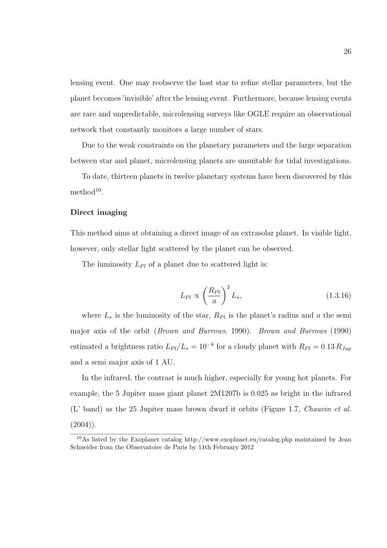
26
lensing event. One may reobserve the host star to refine stellar parameters, but the
planet becomes ’invisible’ after the lensing event. Furthermore, because lensing events
are rare and unpredictable, microlensing surveys like OGLE require an observational
network that constantly monitors a large number of stars.
Due to the weak constraints on the planetary parameters and the large separation
between star and planet, microlensing planets are unsuitable for tidal investigations.
To date, thirteen planets in twelve planetary systems have been discovered by this
method10.
Direct imaging
This method aims at obtaining a direct image of an extrasolar planet. In visible light,
however, only stellar light scattered by the planet can be observed.
The luminosity LPl of a planet due to scattered light is:
LPl ∝(RPl
a
)2
L∗, (1.3.16)
where L∗ is the luminosity of the star, RPl is the planet’s radius and a the semi
major axis of the orbit (Brown and Burrows, 1990). Brown and Burrows (1990)
estimated a brightness ratio LPl/L∗ = 10−8 for a cloudy planet with RPl = 0.13RJup
and a semi major axis of 1 AU.
In the infrared, the contrast is much higher, especially for young hot planets. For
example, the 5 Jupiter mass giant planet 2M1207b is 0.025 as bright in the infrared
(L’ band) as the 25 Jupiter mass brown dwarf it orbits (Figure 1.7, Chauvin et al.
(2004)).
10As listed by the Exoplanet catalog http://www.exoplanet.eu/catalog.php maintained by JeanSchneider from the Observatoire de Paris by 11th February 2012

27
Figure 1.7: Composite image of the brown dwarf 2M1207 and its gas giant companionin the infrared (Chauvin et al., 2004).
This detection method is sensitive to young hot planets (a few tens of million
years old) around faint stellar or substellar objects. This work, however, focuses
on older systems whose stars have settled on the main sequence. Furthermore, the
planets found by direct imaging are so far away from their star that tidal interactions
between them are negligible.
To date, 31 planets in 27 planetary systems have been discovered by direct imag-
ing11.
Transit method
The transit method aims for the detection of the shallow dip in a photometric
lightcurve of a star caused by the transit of a planet (Figure 1.8). The depth of
11As listed by the Exoplanet catalog http://www.exoplanet.eu/catalog.php maintained by Jean

28
Figure 1.8: As the planet passes in front of its star, the apparent brightness of thestar decreases by ∆F (Credit: Hans Deeg, ESA).
a transit DTransit is determined by the following ratio:
DTransit =∆F
F=
(RPl
R∗
)2
, (1.3.17)
where F is the observed mean flux before and after the transit, ∆F is the flux differ-
ence during transit and RPl and R∗ are the planet’s and star’s radius, respectively.
When the spectral type of the star is known, the planet’s radius can be inferred
immediately. This is the only method that yields the radius of a planet so far.
The transit detection requires accurate star flux monitoring, as can be shown by
calculating the transit depth DTransit for Solar System planets: The Jupiter transit
leads to a ≈ 1% reduction of the solar flux, the Neptune transit reduces the solar flux
by 0.13% and the Earth transit by 0.0084%.
A transit, however, is only visible if the line-of-sight is parallel or nearly parallel
to the orbital plane of the planet (i ≈ 90 ) (Figure 1.9). Let γ be the angle between
two rays from the top of the star and the bottom of the star of radius R∗ that meet
the planet at semi major axis aPl. The same rays span a sphere segment S at distance
aPl + y between star and observer on Earth.
Schneider from the Observatoire de Paris by 11th February 2012

29
Figure 1.9: Probability to observe a transit from Earth.
The probability PTransit to observe a transit is the ratio of the small segment
2π(y+aPl)S, within which the transit is visible, over the whole sphere surface 4π(y+
aPl)2. Because y ≫ aPl and with the relations S = γy and 2R∗ = γaPl, the following
equation is derived for PTransit:
PTransit =R∗
aPl
. (1.3.18)
The Earth has a 0.42% probability to be observed by a transit by a distant observer,
for Jupiter the probability is even less: PTransit ≈ 0.1%. For planets like 51 Pegasi
b with aPl ≈ 0.05 AU and a host star of radius R∗ ≈ RSun, the probability is about
10%. Therefore, the transit method predominantly finds large planets in close orbits.
These represent 10% of the total planet population, assuming that planetary orbits
can assume any inclination with respect to the line-of-sight.

30
The probability to observe a transit event is relatively small. Therefore, observa-
tion programs that use the transit method, like the CoRoT and Kepler space missions,
monitor a large number of stars to maximize their yields of transiting planets. CoRoT,
for example, observes ≈ 10 000 stars per star field every six months (Carone et al.
(2011) among others).
Every transit detection has to be confirmed by radial velocity measurements (Sec-
tion 1.3.1), because the mass of the planet can not be determined by the transit
method. A combination of both methods yields the full parameter set of the system:
true planetary massMPl, planetary radius RPl, semi major axis a, eccentricity e, and
even the density of a planet which is important to determine its composition.
The full set of planetary parameters and a good knowledge of stellar parameters
like the age of the system and the stellar rotation period are very important for the
investigations of tidal interactions between extrasolar planets and their host stars
discussed in this work. The parameters of planetary systems detected by the transit
method, especially those found by the space mission CoRoT, are very well determined
and therefore this work focuses on these planets. The space mission Kepler also
provided several exoplanets suitable for tidal interaction investigations, but at the
time of the writing, the parameters of many Kepler.planets and their host stars were
still under investigation. CoRoT-planets benefit from the fact that the CoRoT mission
was launched several years earlier.
To date, 230 transiting planets have been found in 196 planetary systems12.
12As listed by the Exoplanet catalog http://www.exoplanet.eu/catalog.php maintained by JeanSchneider from the Observatoire de Paris by 11th February 2012
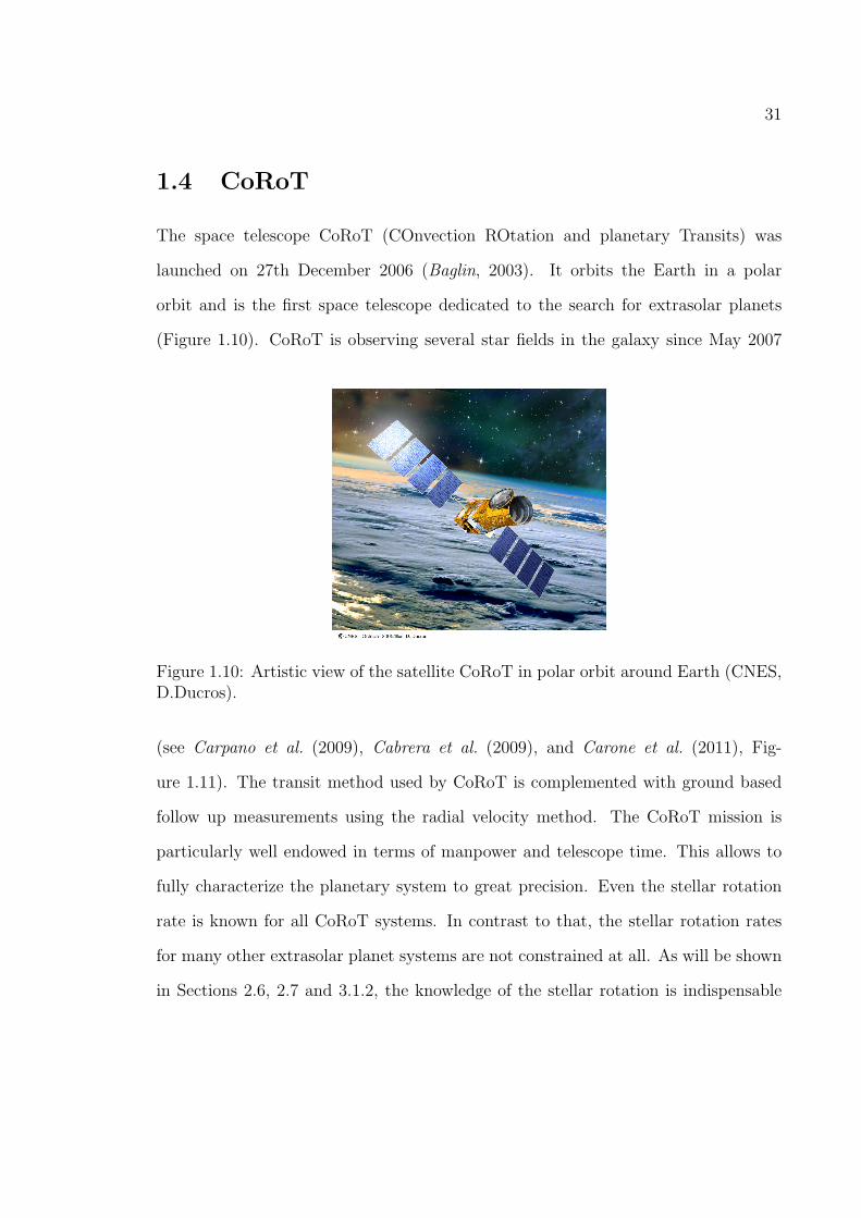
31
1.4 CoRoT
The space telescope CoRoT (COnvection ROtation and planetary Transits) was
launched on 27th December 2006 (Baglin, 2003). It orbits the Earth in a polar
orbit and is the first space telescope dedicated to the search for extrasolar planets
(Figure 1.10). CoRoT is observing several star fields in the galaxy since May 2007
Figure 1.10: Artistic view of the satellite CoRoT in polar orbit around Earth (CNES,D.Ducros).
(see Carpano et al. (2009), Cabrera et al. (2009), and Carone et al. (2011), Fig-
ure 1.11). The transit method used by CoRoT is complemented with ground based
follow up measurements using the radial velocity method. The CoRoT mission is
particularly well endowed in terms of manpower and telescope time. This allows to
fully characterize the planetary system to great precision. Even the stellar rotation
rate is known for all CoRoT systems. In contrast to that, the stellar rotation rates
for many other extrasolar planet systems are not constrained at all. As will be shown
in Sections 2.6, 2.7 and 3.1.2, the knowledge of the stellar rotation is indispensable

32
Figure 1.11: The CoRoT ’eyes’ in the night sky (diameter:10). The ’red’ circleis observed in summer and contains the Aquila constellation. The ’blue’ circle isobserved in winter and lies in the Monoceros constellation (CNES).
Planet type CoRoT planetGas Giant CoRoT-1b, CoRoT-2b, CoRoT-4b, CoRoT-5b, CoRoT-
6b, CoRoT-8b, CoRoT-9b, CoRoT-10b, CoRoT-11b,CoRoT-12b, CoRoT-13b, CoRoT-14b, CoRoT-16b,CoRoT-17b, CoRoT-18b, CoRoT-19b, CoRoT-20b,CoRoT-21b
Brown Dwarf CoRoT-3b, CoRoT-15bSuper Earth CoRoT-7b
Table 1.1: Planet types discovered by the CoRoT space mission.
for the investigation of tidal interactions. At the time of writing, the full parameter
set of twenty-one CoRoT planetary systems is known. Table 1.1 lists the gas giant
planets, brown dwarfs and terrestrial planets found by the CoRoT space mission. The
stellar and planetary parameters are given in Tables 1.2 and 1.3, respectively. The
stellar rotation period and planetary revolution period are listed in Table 1.4. The
references for each system are listed in the Appendix (Table A.1).
As can be seen from Table 1.1, many CoRoT planets are massive companions like
gas giants and brown dwarfs with small semi major axes. Even one Super Earth,

33
CoRoT-7b, with an extremely close orbit was discovered. Therefore, the CoRoT
planets provide an interesting test field for the investigation of tidal interactions with
very well determined parameters.
Furthermore, the author’s working group is directly involved in the CoRoT mission
and therefore the author had access to data in the proprietary phase (see Grziwa et al.
(2012) for a description of the analysis of CoRoT data). The data for the CoRoT
planets CoRoT-19b-21b were, for example, not public at the time of writing. In
addition, the CoRoT planets present several interesting tidal interaction scenarios,
as will be shown in Chapter 4, that allow a consistent comparative analysis of tidal
interactions in planetary systems from a single data source.

34
Systems Spectraltype
Stellar Mass Stellar Radius Stellar Ro-tation Pe-riod
Stellar Age
[MSun] [RSun] [days] [Gyrs]CoRoT-1 G0V 0.95± 0.15 1.11± 0.05 10.8+2.6
−1.8 -CoRoT-2 G7V 0.97± 0.06 0.902± 0.018 3.85± 0.17 0.5+3.5
−0.3
CoRoT-3 F3V 1.37± 0.09 1.56± 0.09 3.85± 0.17 1.6− 2.8CoRoT-4 F8V 1.1± 0.03 1.15± 0.03 9.2+1.7
−1.3 0.7− 2CoRoT-5 F9V 1± 0.2 1.19± 0.04 > 30 5.5− 8.3CoRoT-6 F9V 1.05± 0.05 1.025± 0.026 7± 1 2.5− 4CoRoT-7 G9V 0.91± 0.03 0.82± 0.04 22+66
−9.4 1.2− 2.3CoRoT-8 K1V 0.88± 0.04 0.77± 0.02 19.5+19.5
−6.5 1.7+0.6−0.5
CoRoT-9 G3V 0.99± 0.04 0.94± 0.04 ≥ 13.6 0.15− 8CoRoT-10 K1V 0.89± 0.05 0.79± 0.05 20+6.6
−4 1− 3CoRoT-11 F6V 1.27± 0.05 1.37± 0.03 1.4± 0.3 1− 3CoRoT-12 G2V 1.08± 0.08 1.12± 0.1 57+∞
−28 3− 9CoRoT-13 G0V 1.09± 0.02 1.01± 0.03 12.8+4.3
−2.6 0.12− 3CoRoT-14 F9V 1.13± 0.09 1.21± 0.08 12.8+4.3
−2.6 0.4− 0.8CoRoT-15 F7V 1.32± 0.12 1.46+0.3
−0.14 3.9± 0.4 1− 3CoRoT-16 G5V 1.1± 0.08 1.19± 0.14 ≥ 60 6.7± 2.8CoRoT-17 G2V 1.04± 0.10 1.59± 0.07 18± 2 10.7± 1.0CoRoT-18 G9V 0.95± 0.15 1.03± 0.10 5.4± 0.4 0.6± 0.4CoRoT-19 F9V 1.21± 0.06 1.65± 0.04 14.0± 2.4 5± 1CoRoT-20 G2V 1.14± 0.08 1.02± 0.05 11.5± 2.6 0.1+0.8
−0.04
CoRoT-21 F8IV 1.29± 0.09 1.95± 0.21 9.0± 2.8 4.1± 0.5
Table 1.2: Stellar parameters of CoRoT-1 to -21.

35
Planet PlanetaryMass
Planetary Ra-dius
Semi Major Axis Orbit Ecc.
[MJ ] [RJ ] [AU ]CoRoT-1b 1.03± 0.12 1.49± 0.08 0.0254± 0.0004 0CoRoT-2b 3.31± 0.16 1.465± 0.029 0.0281± 0.0009 0CoRoT-3b 21.66± 1 1.01± 0.07 0.057± 0.003 0CoRoT-4b 0.72± 0.08 1.19± 0.06 0.090± 0.001 0− 0.1CoRoT-5b 0.467+0.047
−0.024 1.39± 0.05 0.0495± 0.0003 0CoRoT-6b 2.96± 0.34 1.166± 0.035 0.0855± 0.0015 < 0.1CoRoT-7b 0.024± 0.004 0.0172±2×10⁻⁴ 0.0172± 0.0002 0CoRoT-8b 0.22± 0.03 0.57± 0.02 0.063± 0.001 0CoRoT-9b 0.84± 0.07 1.05± 0.04 0.407± 0.005 0.11± 0.04CoRoT-10b 2.75± 0.16 0.97± 0.07 0.1055± 0.0021 0.53± 0.04CoRoT-11b 2.33± 0.34 1.43± 0.03 0.044± 0.005 0CoRoT-12b 0.92± 0.07 1.44± 0.13 0.04016± 0.0009 0.07+0.06
−0.04
CoRoT-13b 1.308± 0.066 0.885± 0.014 0.051± 0.003 0CoRoT-14b 7.6± 0.6 1.09± 0.07 0.027± 0.002 0CoRoT-15b 63.3± 4.1 1.12+0.3
−0.15 0.045± 0.01 0CoRoT-16b 0.535± 0.085 1.17± 0.16 0.0618± 0.0015 0.3± 0.1CoRoT-17b 2.45± 0.16 1.02± 0.07 0.0461± 0.0080 0CoRoT-18b 3.47± 0.38 1.31± 0.18 0.0295± 0.016 < 0.08CoRoT-19b 1.14± 0.05 1.45± 0.05 0.0518± 0.0008 0.047± 0.045CoRoT-20b 4.24± 0.23 0.84± 0.04 0.092± 0.021 0.562± 0.013CoRoT-21b 2.53± 0.37 1.30± 0.04 0.0417± 0.011 0
Table 1.3: Planetary parameters of CoRoT-1b to -21b.

36
System Stellar Rotation Period Planetary Revolution Period[days] [days]
CoRoT-1 10.8+2.6−1.8 1.5089557± 6.4 · ×10−6
CoRoT-2 3.85± 0.17 1.7429964± 1.7× 10⁻⁶
CoRoT-3 3.85± 0.17 4.2568± 5× 10⁻⁶
CoRoT-4 9.2+1.7−1.3 9.20205± 0.00037
CoRoT-5 60+∞−30 4.037896± 1× 10⁻⁶
CoRoT-6 7± 1 8.886593± 4× 10⁻⁶
CoRoT-7 22+66−9.4 0.85359± 0.00059
CoRoT-8 19.5+19.5−6.5 6.21229± 3× 10⁻⁵
CoRoT-9 ≥ 13.6 95.2738± 0.0014CoRoT-10 20+6.6
−4 13.2406± 0.0002CoRoT-11 1.4± 0.3 2.99433± 1× 10⁻⁵
CoRoT-12 57+∞−28 2.82805± 5× 10⁻⁴
CoRoT-13 12.8+4.3−2.6 4.03519± 3× 10⁻⁵
CoRoT-14 12.8+4.3−2.6 1.51214± 1.3× 10⁻⁴
CoRoT-15 3.9± 0.4 3.06036± 3× 10⁻⁵
CoRoT-16 ≥ 60 5.35227± 0.00020CoRoT-17 18± 2 3.76813± 0.00026CoRoT-18 5.4± 0.4 1.9± 2.8× 10⁻⁶
CoRoT-19 14.0± 2.4 3.89713± 1× 10⁻⁵
CoRoT-20 11.5± 2.6 9.244± 0.001CoRoT-21 9.0± 2.8 2.72474± 0.00014
Table 1.4: Stellar rotation period of CoRoT-1 to -21 and planetary revolution ofCoRoT-1b to -21b.

37
1.5 Overview of exoplanet properties
An overview of the extrasolar planet systems discovered so far and their properties
are presented. Special emphasis is put on the relevance of the systems’ properties for
tidal interactions between the planets and their host stars13.
Figure 1.1 shows the mass distribution of all known extrasolar planets. The ex-
istence of the brown dwarf desert is apparent: There is a deficiency of substellar
companions more massive than thirteen Jupiter masses although they are much eas-
ier to detect. There is no shortage, on the other hand, of Jupiter mass planets, which
are ideal candidates to test their influence on their host stars due to tidal forces.
Figure 1.12 contains the distribution of the exoplanets’ mass on logarithmic scale.
Figure 1.12: Histogram of the masses of all detected exoplanets in logarithmic scale.
13The parameters were taken once again from the Exoplanet cataloghttp://www.exoplanet.eu/catalog.php maintained by Jean Schneider from the Observatoirede Paris.
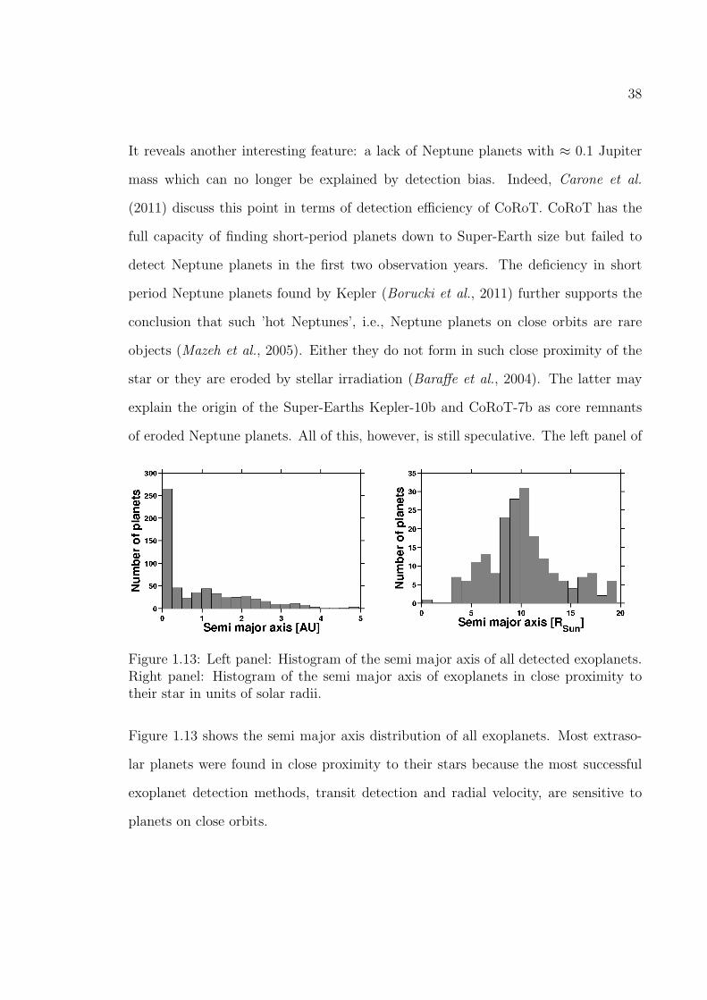
38
It reveals another interesting feature: a lack of Neptune planets with ≈ 0.1 Jupiter
mass which can no longer be explained by detection bias. Indeed, Carone et al.
(2011) discuss this point in terms of detection efficiency of CoRoT. CoRoT has the
full capacity of finding short-period planets down to Super-Earth size but failed to
detect Neptune planets in the first two observation years. The deficiency in short
period Neptune planets found by Kepler (Borucki et al., 2011) further supports the
conclusion that such ’hot Neptunes’, i.e., Neptune planets on close orbits are rare
objects (Mazeh et al., 2005). Either they do not form in such close proximity of the
star or they are eroded by stellar irradiation (Baraffe et al., 2004). The latter may
explain the origin of the Super-Earths Kepler-10b and CoRoT-7b as core remnants
of eroded Neptune planets. All of this, however, is still speculative. The left panel of
Figure 1.13: Left panel: Histogram of the semi major axis of all detected exoplanets.Right panel: Histogram of the semi major axis of exoplanets in close proximity totheir star in units of solar radii.
Figure 1.13 shows the semi major axis distribution of all exoplanets. Most extraso-
lar planets were found in close proximity to their stars because the most successful
exoplanet detection methods, transit detection and radial velocity, are sensitive to
planets on close orbits.

39
Figure 1.14: Left panel: Histogram of the masses of all detected transiting exoplan-ets. Right panel: Histogram of the masses of all detected transiting exoplanets inlogarithmic scale.
It will be shown in the next chapter that the smaller the semi major axis and the
greater the mass of the planet, the stronger the tidal forces acting on the planet and
on the star. The distribution of the semi major axes of the exoplanets in very close
proximity to their star (Figure 1.13, left panel) is not flat but peaks at 10 solar radii.
The slope between 1 and 10 solar radii may hint at an erosion of such very massive
extrasolar planets due to tidal forces.
This work focuses on transiting planets because for these the stellar and planetary
parameters, particularly the planet’s mass, are known to a better degree than for
planets discovered by other methods. Figure 1.14 shows their mass distribution and
Figure 1.15 shows their semi major axes distribution. Again, the majority of the
transit planets are Jupiter-like with a deficiency of Neptune planets. About two
hundred transiting planets orbit in very close proximity to their star, making them
an ideal target for the investigations of tidal interactions.
The fact that so many close-in extrasolar planets proves the relevance of the
investigation of orbital stability due to tidal interactions.

40
Figure 1.15: Left panel: Histogram of the semi major axis of all detected transitingexoplanets. Right panel: Histogram of the semi major axis of transiting exoplanetsin units of solar radii.

Chapter 2
Theory of tidal interaction
The theoretical framework necessary to describe tidal forces will be presented. Special
emphasis will be put on potential theory and the mathematical description of radial
symmetric potentials in polar coordinates. It will be shown that extended bodies
are deformed by tidal forces and that energy is dissipated within them. This leads
to tidal friction which may change a planet’s orbit and a star’s rotation in secular
time scales. The relevant equations will be derived for circular as well as for eccentric
orbits.
A quick overview will be given on the timescales on which tidal friction acts in the
Solar System and on the uncertainties of tidal friction timescales in exoplanet systems.
The special case of the equilibrium state under tidal friction will be presented and its
stability will be discussed. Furthermore, the angular momentum evolution of main
sequence stars and their moment of inertia will be presented, as both are needed to
model stellar rotation evolution. Finally, the Roche limit is discussed. This is the
distance at which a planet is tidally disrupted.
41

42
2.1 The gravitational potential
The gravitational potential for a point mass and an extended uniform sphere will be
calculated (according to Kertz (1969)) to prepare the calculation of an extended body
with an arbitrary mass distribution.
For a point mass M , the gravitational force at a distance r′ is described by New-
ton’s law of gravity:
FGravity(r) =GM
r′2r, (2.1.1)
where G = 6.673× 10⁻¹¹ m3
kgs2is the gravitational constant and r is the unit vector
of the position vector r′ of the reference point in a coordinate system with the point
mass as its origin.
The corresponding gravitational potential is:
Φ(r) = −GMr′
. (2.1.2)
For an extended body, a mass distribution∫
dm needs to be considered.
In the following, the coordinates of a potential reference point in polar coordinates
are r′, θ′, ϕ′, the coordinates of a mass element dm are r, θ, ϕ.
2.1.1 The outer gravitational potential
The easiest case to consider is that of the gravitational potential of a homogeneous
sphere of total massM with radius R and constant density ρ as seen from a reference
point P ′ at distance r′ ≥ R is (r′ is measured from the center of mass):
ΦGravity(r′) = −
∫M
G dm
∆, (2.1.3)

43
Figure 2.1: The parameters of the mass element dm in polar coordinates.
where dm is a mass element at distance r ≤ R from the center of mass and ∆ is the
distance between the mass element dm and the reference point.
For the mass element dm at position P the following holds in polar coordinates:
dm = ρdV = ρ · dr · r dθ · r sin θ dϕ, (2.1.4)
where r is the radial distance from the center of mass, θ is the colatitude measured
from the polar axis and ϕ is the longitude (Figure 2.1).

44
Figure 2.2: The distance ∆ between P , the position of the mass element dm, andthe reference point P ′ in polar coordinates
For the distance ∆ the following holds (Figure 2.2):
∆2 = r′2 + r2 − 2r′r cos θ. (2.1.5)
According to this, dθ can be substituted by d∆:
2∆d∆ = 2rr′sinθ dθ. (2.1.6)
The outer gravitational potential is now:
ΦGravity(r′) = −Gρ
∫ R
0
∫ π
0
∫ 2π
0
r2 sin θ
∆dr dθ dϕ (2.1.7)
= −G2πρ
r′
∫ R
0
r
(∫ r′+r
r′−r
d∆
)dr
= −Gρ4πR3
3r′,

45
which is equal to the potential of a point massM at the center of mass of the extended
body because ρ4πR3
3= ρ · VSphere =M .
2.1.2 Inner gravity potential
The inner potential of a homogeneous sphere of radius R, mass M and density ρ is
derived as seen from a reference point P ′ at distance r′ < R from the center of mass
(again according to Kertz (1969)). It is useful to decompose the inner potential by
considering the gravity potential of an inner homogeneous sphere of radius r and the
remaining gravity potential of a spherical shell of thickness R− r′.
For the potential ΦI(r′) of the inner sphere the result of (2.1.7) is used. Here,
the reference point lies on the surface of the inner sphere (RI = r′) and therefore the
potential is:
ΦI(r′) = −Gρ4πr
′2
3= −GMr′2
R3, (2.1.8)
where ρ was substituted by 3M4πR3 .
For the second part of the inner gravitational potential ΦR(r′), the potential of a
homogeneous spherical shell, the following holds:
ΦR(r′) = −Gρ
∫ R
r′
∫ π
0
∫ 2π
0
r2 sin θ
∆dr dθ dϕ (2.1.9)
= −G2πρ
r′
∫ R
r′r
(∫ r+r′
r−r′d∆
)dr
= −G2πρ(R2 − r′2
).
Consequently, the total internal gravitational potential of a homogeneous sphere is:
Φint(r) = ΦI(r′) + ΦR(r
′) = −2
3πρG(3R2 − r′2) (2.1.10)

46
The homogeneous spherical sphere is a very special case. It is, however, useful as a
first approximation.
2.2 The role of Legendre polynomials in axial sym-
metric gravity potentials
In general, the gravitational potential of an extended body of arbitrary shape with
inhomogeneous density distribution as seen from a point P ′ is the sum over the
potential of all point massesmi (the derivation was adapted fromMurray and Dermott
(1999)):
Φgravity,body(r′) = G
∑i
mi
∆(2.2.1)
or
Φgravity,body(r′) = G
∫V
ρ(Pi)
∆dVi, (2.2.2)
where ρ(Pi) is the density of the volume element dVi at a point Pi inside the body with
the coordinates (ri = ri, θi, ϕi). ∆ is the distance between the mass element dmi =
ρ(Pi) dVi and the point of reference P ′ with the coordinates (r′ = r′, θ′, ϕ′)(Figure
2.3). ∆ can be described in terms of ri and r′ as:
∆2 = r2i + r′2 − 2r′ri cos(χ), (2.2.3)
where χ is the angle between the vectors r and ri. The term 1/∆ can be expanded
binomially either with respect to r′ or with respect to ri:
1
∆=
1
r′
∞∑l=0
Pl(cosχ)(rir′
)lif ri ≤ r′
1
ri
∞∑l=0
Pl(cosχ)
(r′
ri
)l
if ri ≥ r′,
(2.2.4)
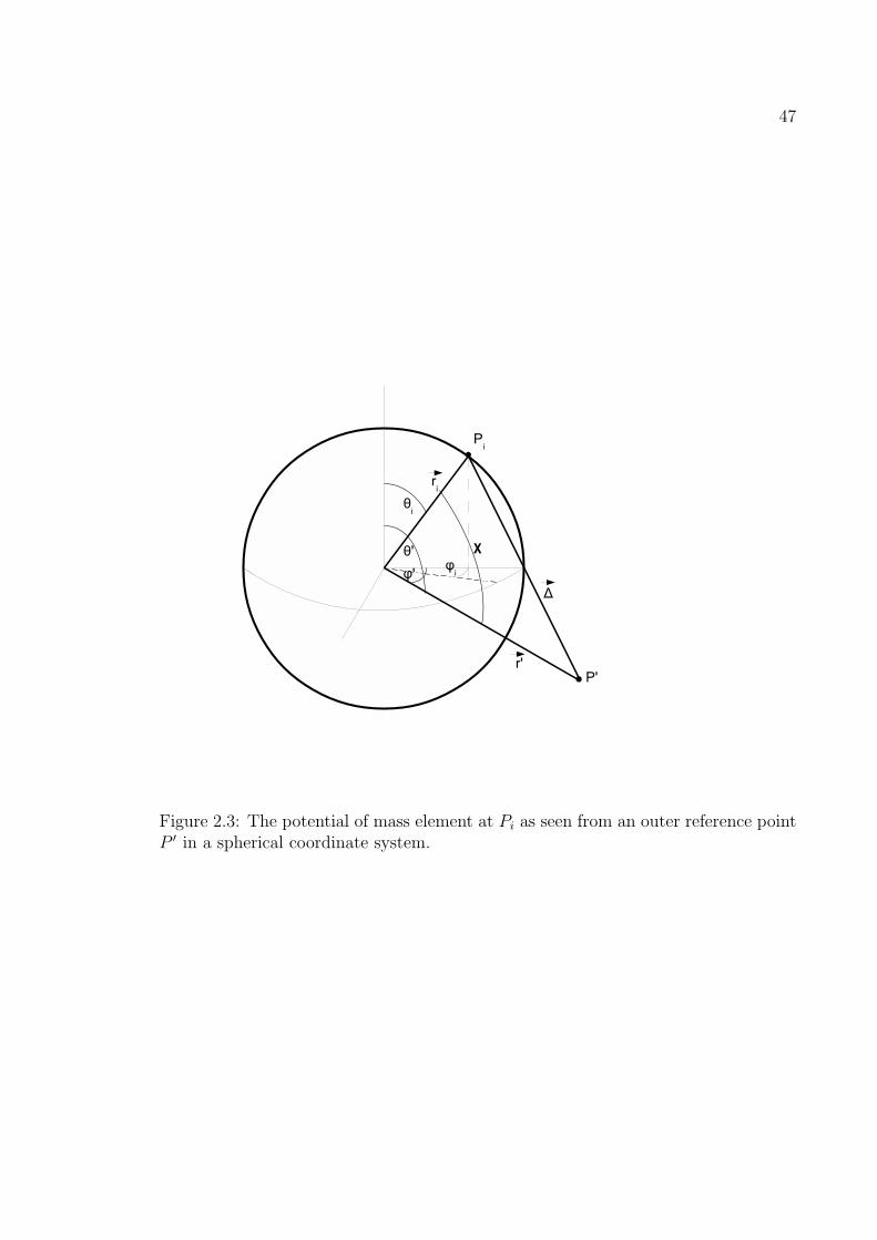
47
Figure 2.3: The potential of mass element at Pi as seen from an outer reference pointP ′ in a spherical coordinate system.

48
where Pl(cosχ) are the Legendre polynomials. They can be calculated using Ro-
drigues’ formula (see Murray and Dermott (1999) among others):
Pl(x) =1
2ll!
dl(x2 − l)l
dxl. (2.2.5)
The Legendre polynomials play an important role in the solution of potentials that
satisfy the Laplace equation. This will be explained in more detail in the following
section and follows the treatment given in Murray and Dermott (1999) and Kertz
(1969).
2.2.1 Potential theory
Laplace’s equation is:
∇2V = 0. (2.2.6)
Transformed into spherical coordinates (r, θ, ϕ), this becomes:
∂
∂r
(r2∂V
∂r
)+
∂
∂µ
((1− µ2)
∂V
∂µ
)+
1
1− µ2
∂2V
∂ϕ2= 0, (2.2.7)
where µ = cos θ.
Any function V that satisfies the equation above can be decomposed into three
functions, each of which depends only on either r, θ or ϕ, respectively. V is called
a spherical solid harmonic. The solution of Laplace’s equation can be derived by
setting V = rnSn(µ, ϕ), which contains two functions, one dependent only on r and
the other dependent only on µ and ϕ. In the end, Sn(µ, ϕ) has to factorize into two
separate functions each dependent on µ and θ, respectively, for V to be a spherical
solid harmonic.
Inserting V = rnSn(µ, ϕ) into Laplace’s equation yields:
∂
∂µ
((1− µ2)
∂Sn
∂µ
)+
1
1− µ2
∂2Sn
∂ϕ2+ n(n+ 1)Sn = 0. (2.2.8)

49
This is Legendre’s equation and the function Sn is called a spherical surface har-
monic of degree n. Legendre’s equation can also be derived from Laplace’s equa-
tion with the trial function V = r−(n+1)Sn(µ, ϕ). Therefore, the general solution of
Laplace’s equation (the spherical solid harmonic) is:
V =∞∑n=0
(Anr
n +Bnr−(n+1)
)Sn(µ, ϕ), (2.2.9)
where An and Bn are constants.
A more detailed treatment of the general solution can be found in Kertz (1969).
In this work, however, axial symmetry is assumed: The situations discussed in the fol-
lowing do not depend on ϕ and consequently (∂2Sn)/(∂ϕ2) = 0. Therefore, Legendre’s
equation reduces to:
(1− µ2)∂2Pn(µ)
∂µ2− 2µ
∂Pn(µ)
∂µ+ n(n+ 1)Pn(µ) = 0. (2.2.10)
The Legendre polynomials Pn(µ) satisfy Laplace’s equation under axial symmetry
and are called zonal surface harmonics.
Surface harmonics have the important property that they are orthonormal and
satisfy the following relation:∫ 2π
0
∫ +1
−1
Ym(µ, ϕ)Sn(µ, ϕ)dµϕ = 0 ifm = n, (2.2.11)
=4π
2n+ 1ifm = n,
where Ym(µ, ϕ) and Sn(µ, ϕ) are two spherical surface harmonics of degree m and
n, respectively. Here, the Schmidt or Gram-Schmidt orthonormalization over a unit
sphere is used. A very useful property of this normalization is described in the
following: Let P and P ′ be two points on a unit sphere with the angular coordinates

50
Figure 2.4: The location of two points P and P ′ on a unit sphere.
(θ, ϕ) and (θ′, ϕ′), respectively, and let χ be the angle between the vectors (r = 1, θ, ϕ)
and (r = 1, θ′, ϕ′) (Figure 2.4). Then:∫ 2π
0
∫ +1
−1
Sn(µ′, ϕ′)Pn(cosχ)dµ
′dϕ′ =4π
2n+ 1Sn(µ, ϕ), (2.2.12)
where µ′ = cos θ′ and µ = cos θ.
Applying this to the gravitational potential of an extended inhomogeneous body of
arbitrary form and choosing a coordinate system such that its origin coincides with the
center of mass, the gravitational potential at a reference point P (r, µ = cos θ, ϕ) can
be described as (see Kertz (1969) and Murray and Dermott (1999) for the derivation):
Φgravity,body(P ) = −GMr
[1−
∞∑n=2
n∑m=0
(R
r
)n
Pmn (cos θ)(Cm
n cos(mϕ) + Smn sin(mϕ))
],
(2.2.13)

51
where
Cmn = − 1
RnM
∫ R
0
dri
∫ 1
−1
dµi
∫ 2π
0
dϕi ρ(Pi)rn+2i Pm
n (µi) cos(mϕi) (2.2.14)
Smn = − 1
RnM
∫ R
0
dri
∫ 1
−1
dµi
∫ 2π
0
dϕi ρ(Pi)rn+2i Pm
n (µi) sin(mϕi), (2.2.15)
are integrated over a mass element dmi at a point Pi(ri, cos θi = µi, ϕi) with density
ρ(Pi) and reflect the mass distribution within an extended body. The associated
Legendre polynomials Pmn are derived from the ordinary Legendre polynomials by:
Pmn (µ) = (−1)m(1− µ2)
m2dmPn(µ)
dµm, (2.2.16)
with m = 0, 1, 2, ...n.
If the potential is axial symmetric with respect to ϕ, then m equals zero. In
this case, the associated Legendre polynomials are equal to the ordinary Legendre
polynomials (P 0n = Pn).
This is the theoretical framework - in terms of potential theory - that is needed
as a basis for describing the tidal interaction between two bodies.
2.3 Tidal force and potential
The following is derived from Murray and Dermott (1999) and Kertz (1969). A situ-
ation is considered where a celestial object experiences tides due to the gravitational
attraction of another body. The first object will be called from now on the primary
and its parameters are denoted by the subscript P . The second object will be referred
to as the secondary and its parameters are denoted by the subscript S. Furthermore,
the mass of the primary is assumed to be much greater than the mass of the sec-
ondary: MP ≫ MS. Both shall orbit a common center of mass that lies within the

52
Figure 2.5: The relationships between the radius of the primary, RP , the radius ofthe orbit of the secondary, a, and the distance ∆ from a point P on the surface ofthe primary to the center of mass of the secondary.
primary. The orbit shall be circular with a radius a. In addition, a is much greater
than the respective radii RP and RS of the primary and the secondary: a ≫ RP
and a ≫ RS. A coordinate system is chosen with its origin at the center of mass of
the primary and the latitude Ψ is measured from the axis that points towards the
secondary (Figure 2.5).
The gravitational field of the secondary at any position P ′ on the surface and
within the primary is indistinguishable from that of a point mass MS. The primary
on the other hand is considered as extended: Mass elements dm at position P ′ within
the primary have different distances ∆ to the origin of the gravitational force, the
center of mass of the secondary. Therefore, the gravitational field as seen from a
reference point P ′ at the surface of the primary with the coordinates (r′ = RP ,Ψ) is
described by:
Φgravity,S(P′) =
GMS
∆, (2.3.1)

53
where ∆ is:
∆ = R2P + a2 − 2R2
Pa cosΨ andRP ≪ a. (2.3.2)
∆ is expanded according to equation (2.2.4). Therefore, the gravity potential that is
felt at the surface of the primary can be described by:
Φgravity,S(P′) = −GMS
a
∞∑l=0
(RP
a
)l
Pl(cosΨ) (2.3.3)
= −GMS
a
[1 +
(RP
a
)cosΨ +
1
2
(RP
a
)2
(3 cos2Ψ− 1) + ...
]≈ V1 + V2 + V3.
Only the leading three terms of the gravitational field are further considered. The
corresponding force of this potential is derived by applying the gradient operator:
Fgravity,S
MP
= −∇Φgravity,S(P′) (2.3.4)
≈ −∇V1 −∇V2 −∇V3.
The gradient of the first term of the potential, −∇V1, is 0, because V1 contains only
constants 1. Only V2 and V3 remain.
At the same time, V2 = −GMS
a2RP cosΨ according to equation (2.3.3). Because
the coordinate system was selected such that one of the axes is pointing along a
(Figure 2.5), the gradient of the potential in the direction RP cosΨ is parallel to a,
pointing towards the secondary. This gradient applied to V2 yields:
− ∂V2∂RP cosΨ
=GMS
a2. (2.3.5)
1Note that this is the viewpoint as seen from a reference point P ′ at any point at the surfaceof the primary. When the position of the reference point changes, ∆ changes as well, but the semimajor axis a is constant in this context.

54
Figure 2.6: Centrifugal versus gravitational force at different points within the pri-mary.
Gravity, however, is not the only force that needs to be considered. Because the
primary and the secondary orbit around a common center of mass, a centrifugal force
due to this motion arises as well. The difference between the centrifugal and the
gravitational force is the tidal force (Figure 2.6).
The properties of the centrifugal force due to the motion of the primary on a grav-
itationally bound orbit is illustrated by Figure 2.7: All particles within the primary
move on congruent circles if rotation is neglected. The corresponding centrifugal
force is acting in the direction of the secondary parallel to a and is the same for every
point within the primary in magnitude and direction. The magnitude of the centrifu-
gal force is known for one point at least: For the center of mass it has to be equal
to GMPMS/a2, the gravitational force between the two point masses MS and MP .

55
Figure 2.7: The particles in a primary move on circles of identical radii aP , which isthe distance from the primary’s center of mass to the common center of gravity CM .This is illustrated by the movement of P ′ about the point CM ′ and the center of theprimary CP about CM . In this picture the rotation of the primary about its polaraxis is neglected.
56
Therefore the force arising due to the potential V2 is compensated by the centrifugal
force at any point within the primary.
When the centrifugal force is subtracted from (2.3.3) only the force arising from
the potential V3 remains. This is the tidal force and V3 is identical to the tidal
potential Vtide:
Vtide(P′) = Φgravity,S − Φcentrifugal (2.3.6)
≈ (V1 + V2 + V3)− Φcentrifugal
= ( V1︸︷︷︸∇V1=0
+ V2︸︷︷︸=Φcentrifugal
+V3)− Φcentrifugal
= V3
= −GMS
a
(ra
)2P2(cosΨ).
The tidal force acting on any mass m within the primary at a reference point P ′
with coordinates r′ = (r′,Ψ) is:
Ftide/m = −∇Vtide
= −∂Vtide∂r′
ˆr′ − 1
r′∂Vtide∂Ψ
ˆΨ
= 2GMS
a3r′P2(cosΨ)
ˆr′ − 2
GMS
a3r′3
4sin(2Ψ)
ˆΨ, (2.3.7)
whereˆr′ and
ˆΨ are the unit vectors in the direction of the r′ and Ψ-axis of the
coordinate system.
At the surface of the primary (r′ = RP ) the tidal potential is:
Vtide(RP ) = −GMSR2P
a3P2(cosΨ) = −ζPgPP2(cosΨ), (2.3.8)
where
1
2
(3 cos2 Ψ− 1
)(2.3.9)

57
is the Legendre Polynomial of degree n = 2 with respect to cosΨ′,
gP =GMP
R2P
(2.3.10)
is the gravitational acceleration on the surface of the primary, and the remaining
terms are combined in ζP :
ζP =MP
MS
(RP
a
)3
·Rp . (2.3.11)
ζPP2(cosΨ) is the amplitude of the equilibrium tide for any angle Ψ on the surface of
the primary. It reaches its maximum for Ψ = 0, π and its minimum for Ψ = π/2, 3π/2.
This explains why the tidal force produces two high tides and two low tides per
rotation cycle.
2.4 Deformation of celestial bodies
2.4.1 Tidal deformation
Up to now, the primary was considered as spherical throughout the whole evaluation
of the potential and forces. The shape of the primary, however, only assumes a
spherical form if homogenous density is assumed and if the primary is only subjected
to self-gravity. As was shown in the previous section, the mass elements of the primary
are not only subjected to the gravitational but also to the tidal potential Vtide. This
leads to a deformation of the primary, which will be elaborated in the following. The
derivation according Murray and Dermott (1999) is given.
The mass elements of the surface are assumed to change their position until all the
forces acting on them are in equilibrium. Therefore, the surface forms an equipotential
surface. In the literature and also in this work, these outermost mass elements are

58
Figure 2.8: The deformation of a homogenous sphere due to the tidal potential.
sometimes called an ’ocean’ because in this context they are assumed to behave like
a fluid.
The total potential at the surface (r′ = RP ) of the primary is:
Vtotal(RP ,Ψ) = −GMp
RP
− ζgP2(cosΨ) + gh(Ψ), (2.4.1)
where h(Ψ) is the height of the equipotential surface dependent on Ψ. It accounts for
the deformation of the primary due to tides. For the surface to be an equipotential
plane, Vtotal(RP ,Ψ) has to be constant and, consequently, h(ψ) ∝ P2(cosΨ) has to
cancel out the ψ-dependency. Therefore, the primary takes the form of a prolate
ellipsoid (like a rugby ball) with its elongated axis pointing towards the secondary
(Figure 2.8).
If the primary would be an inflexible sphere covered by a shallow, zero-density
fluid, then the surface would be equal to the equilibrium tide h(ψ) = ζP2(cosΨ). In

59
reality, however, the deformation h(ψ) is not the equilibrium tide but deviates from
this ideal form due to the self-gravity of the tidal bulge and the flexibility of the inner
structures of the primary.
In general, the shape of a tidally deformed body is described by:
R(Ψ) = RP [1 + ϵP2(cosΨ)] , (2.4.2)
where ϵ≪ 1 is a constant and ϵP2(cosΨ) is the true amplitude of the tidal bulge.
In addition, a flexible primary will change its mass distribution due to the tidal
deformation. Therefore, its gravitational potential at the surface can no longer be
described by Vgravity,undisturbed = GMP/RP .
To calculate the new gravitational potential as seen from point P (Figure 2.8)
with the coordinates (r, µ = cos θ, ϕ), the deviation from the sphere with radius
Rmean = RP (the ’old’ surface) is considered. The point P ′(r′, µ′ = cos θ′, ϕ′) on the
tidally deformed surface can lie beneath or above the surface of this sphere. The
colatitudes θ, θ′ are this time measured from the axis of symmetry of the tidal bulge
which points towards the secondary (Figure 2.8).
Let χ be the angle between the position vectors to P and P ′. The total gravi-
tational potential at point P can therefore be decomposed into several parts. First,
into the internal and external gravity potential of a spherical body of radius Rmean
(equations 2.1.7 and 2.1.10). Second, into the potential of the non-centric part of a
thin layer of matter between the surface of the deformed body and the mean sphere,
which needs to be added, when this layer lies above the mean radius, and which needs
to be subtracted, when the layer lies below the mean radius.
At P ′, the radial thickness of this thin layer is according to equation (2.4.2) dr′ =
ϵRmeanP2(µ′) and r′ = Rmean. The element of volume at this point is r′2 dr′ dµ′ dϕ′ =
60
ϵR3meanP2(µ
′) dµ′ dϕ′. The distance between the points P and P ′ is ∆ which again
can be expanded binomially (see equation 2.2.4).
Because the height of the tidal bulge can lie either beneath or above Rmean, two
cases are considered.
Case 1: Here, the internal potential of the non-central deformed mass distribution
is derived. Because r < Rmean holds, ∆ = PP ′ can expanded as:
1
∆=(R2
mean + r2 − 2Rmeanr cosχ)−1/2
(2.4.3)
=1
Rmean
∞∑n=0
(r
Rmean
)n
Pn(cosχ).
Therefore, the internal gravitational potential due to the tidal bulge is:
Vint ,bulge = −Gdm∆
(2.4.4)
= −GρR2meanϵ
∞∑n=0
(r
Rmean
)n ∫ ∫P2(µ
′)Pn(cosχ) dµ′ dϕ′
= −GρR2meanϵ
(r
Rmean
)24π
5P2(cos θ)
= −4π
5ρGr2ϵP2(cos θ).
The second last step in the calculations above follows from the special properties of
the spherical harmonics given by equations (2.2.11) and (2.2.12).
The total internal potential of a roughly spherical but tidally deformed body is:
Vint,total(r, θ) = Vint,bulge(r, θ) + Φint(r) (2.4.5)
= −4
3πR3
meanρG
[3R2
mean − r2
2R3mean
+3r2ϵP2(cos θ)
5R3mean
]Case 2: Equivalently, the outer potential is derived (r > Rmean). ∆ = PP ′ can
then be expanded as follows:
1
∆=
1
r
∞∑n=0
(Rmean
r
)n
Pn(cosχ), (2.4.6)

61
Figure 2.9: The tidal deformation of a two-component model planet of radius Rmean
and density ρo and a core of radius RCore and density ρc.
and the total external potential is:
Vext,total(r, θ) = −4
3πR3
meanρG
[1
r+
3R2mean
5r3ϵP2(cos θ)
]. (2.4.7)
From the internal and external gravitational potential of a tidally deformed body, the
true height h(ψ) of the equipotential plane can be derived for a two-component planet
of mean radius Rmean that consists of a homogenous, incompressible, fluid ocean of
density ρO, and a homogeneous core of radius RCore with density ρC . The core is
assumed to be a solid body (Figure 2.9). To form equipotential planes, the shape of
the core boundary and the ocean surface must have the following forms, where Ψ is
measured again from the axis pointing towards the secondary:
RCB(Ψ) = RCore [1 + S2P2(cosΨ)] (2.4.8)
ROS(Ψ) = Rmean [1 + T2P2(cosΨ)] , (2.4.9)

62
where S2 ≪ 1 and T2 ≪ 1 are constants. Furthermore, ζC is the amplitude of the
equilibrium tide at the core boundary:
ζC =MS
MC
(RCore
a
)3
RCore, (2.4.10)
where MC is the mass of the tidally deformed core of the primary. The gravity
acceleration gC at the core boundary is:
gC =GMC
R2Core
(2.4.11)
and µ, the effective rigidity, is a dimensionless constant defined as:
µ =19µ
2ρCgCRCore
, (2.4.12)
where µ is the modulus of rigidity which is defined as the ratio of shear stress to shear
strain. If µ ≪ 1, the core acts like a liquid, if µ ≫ 1 the core hardly deforms at all
under tidal deformation because elastic forces put up too much resistance.
The complete calculations of the tidal deformation of a two-component planet can
be found in Murray and Dermott (1999).
In this two component model, the amplitudes of the tides in the core and in an
outer ocean are:
RCoreS2 = F(5/2)ζC1 + µ
(2.4.13)
RmeanT2 = H5ζ
2, (2.4.14)
where F is a dimensionless number which quantifies the effect of the ocean on the
amplitude of the core tide. H is the effect of the internal structure (elastic forces,
gravitational forces) on the external shape of the whole body.

63
F and H are in general:
F =(1 + µ)(1− ρO/ρC)(1 +
3
2α)
1 + µ− ρO/ρC + (3ρO/2ρC)(1− ρO/ρC)− 94α(RCore/Rmean)5(1− ρO/ρC)2
(2.4.15)
H =2⟨ρ⟩5ρC
1 + µ+ 3
2
(RCore
Rmean
)2
Fδ
(1 + µ)(δ + 2ρO/5ρC)
, (2.4.16)
where < ρ >=MP/(4/3πR3mean) is the mean density,
α = 1+(5ρC)/(2ρO) (RCore/Rmean)3 (1− ρO/ρC)
3 and δ = (RCore/Rmean)3 (1− ρO/ρC)
(Murray and Dermott, 1999).
With this general relation, several special cases can be calculated. For example,
when the core and the shallow ocean have the same density (ρC = ρO) then F = 0
and H = 1. The ocean tide is maximal, 2.5 times the amplitude of the equilibrium
tide:
Rmean(T2 − S2) =5
2ζ, (2.4.17)
and the core is undeformed (S2 = 0).
If a primary has a large solid core and a shallow ocean (Rcore ≈ Rmean, ζc ≈ ζ),
then the following can derived from the two-component model.
The amplitude of the ocean tide is:
Rmean(T2 − S2) =µζ
1− ρOρC
+ µ(1− 3
5ρOρC
) . (2.4.18)
Furthermore, if µ → 0 then the amplitude of the ocean tide approaches zero as
well. The core is maximally deformed and the ocean just follows the form of the core.

64
The amplitude of the solid body tide, on the other hand, is RCoreS2. In the case
of a shallow ocean (Rcore ≈ Rmean), this is:
RmeanS2 =5
2ζ
1− ρOρC
1− ρOρC
+ µ(1− 3ρO
5ρC
) . (2.4.19)
If the planet is ocean-free, then ρO = 0 and the solid body tide is:
RmeanS2 =5
2
ζ
1 + µ, (2.4.20)
which agrees with the expression derived by Lord Kelvin (Thomson, 1863a,b).
2.4.2 Rotational Deformation
The mathematical framework for describing tidal deformation is also useful for de-
scribing rotational deformation. Here again the description in Murray and Dermott
(1999) is used. It is assumed that the tidal as well as the rotational deformations
are small, such that they can be calculated independently and added to each other
linearly (Dermott, 1979a).
At first, a spherical rigid body rotating with angular rotation rate Ω about the
polar axis is investigated (Figure 2.10). Again, axial symmetry with respect to ϕ is
assumed. Consequently, the centrifugal potential depends on r and θ only, where θ is
measured from the polar axis of rotation this time. Note that this coordinate system
differs from the one previously used where θ was measured from an axis pointing
towards the secondary.
The centrifugal potential Vcf (r, θ) at a point P (r, θ) is:
Vcf (r, θ) = −1
2Ω2r2 sin2 θ. (2.4.21)
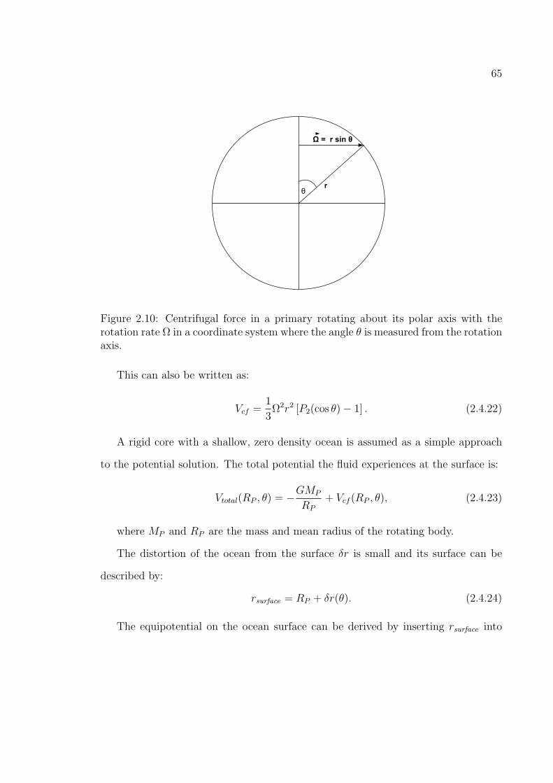
65
Figure 2.10: Centrifugal force in a primary rotating about its polar axis with therotation rate Ω in a coordinate system where the angle θ is measured from the rotationaxis.
This can also be written as:
Vcf =1
3Ω2r2 [P2(cos θ)− 1] . (2.4.22)
A rigid core with a shallow, zero density ocean is assumed as a simple approach
to the potential solution. The total potential the fluid experiences at the surface is:
Vtotal(RP , θ) = −GMP
RP
+ Vcf (RP , θ), (2.4.23)
where MP and RP are the mass and mean radius of the rotating body.
The distortion of the ocean from the surface δr is small and its surface can be
described by:
rsurface = RP + δr(θ). (2.4.24)
The equipotential on the ocean surface can be derived by inserting rsurface into

66
equation (2.4.23) and using a Taylor approximation for terms depending on RP + δr:
Vtotal(surface) ≈ −GMP
RP
+GMP
R2P
δr(θ)− 1
2Ω2R2
P sin2 θ − Ω2RP sin2 θδr(θ). (2.4.25)
If Ω2RP ≪ GMP/R2P , the last term can be neglected and the equation above solved
for δr yields:
δr ≈ const +Ω2R4
P
2GMP
sin2 θ. (2.4.26)
It is obvious that the rotation of a spherical body about its polar axis will deform it
to an oblate ellipsoid. The flattening of such an ellipsoid is defined as:
f =req − rpole
req, (2.4.27)
where the equatorial radius is
req ≈ RP + δr(θ = π/2, 3π/2) + const = RP +Ω2R4
P
2GMP
+ const (2.4.28)
and the polar radius is
rpole ≈ RP + δr(θ = 0, π) + const = RP + const. (2.4.29)
Therefore, the flattening is approximately:
f ≈ q/2 (2.4.30)
where
q =Ω2R3
P
GMP
(2.4.31)
is the dimensionless ratio of the centrifugal to the gravitational acceleration at the
equator. The upper limit of the rotation rate of a planet is derived when q → 1.
Then equation (2.4.31) yields:

67
ΩMax ≈(GMP
R3P
)1/2
≈ 2 · (G⟨ρ⟩)1/2, (2.4.32)
where < ρ > is the mean density of the planet.
Up to now, the gravitational potential at the surface of the rotating planet was
set equal to that of a rigid sphere. This approach neglects feedback effects on the
gravitational potential due to the rotational deformation. Now, an improved model
of the gravitational potential will be derived taking into account the oblate ellipsoidal
form.
The external gravitational potential of such an axially symmetric ellipsoid is (equa-
tion 2.2.13 with m = 0):
Φrot(r, θ) = −GMP
r
[1−
∞∑n=2
Jn
(RP
r
)n
Pn(cos θ)
](2.4.33)
where MP is the total mass, RP is the radius and Jn are dimensionless constants
that describe the mass distribution within the body. Pn(cos θ) is the Legendre poly-
nomial of degree n.
In general, values for Jn are calculated by:
Jn =1
RnPMP
∫ RP
0
∫ +1
−1
rnPn(µ = cos θ)ρ(r, µ)2πr2 dµ dr, (2.4.34)
where ρ(r, µ) describes the internal density distribution. For roughly spherical bodies
like stars and planets several simplifications can be made: If the northern and southern
hemispheres are symmetric, then J3 = 0, J5 = 0, J7 = 0.... J2 is the leading term of
the Jn-terms,. Indeed, if q is small, Jn ∝ qn/2 and higher order terms of Jn can be
neglected.
Also, for a planet of uniform density, J2 = q/2, and for a body of arbitrary density
68
according to MacCullaugh’s theorem (Mayor and Queloz, 1995):
J2 =C − 1/2(A+B)
MPR2P
≈ C − A
MPR2P
, (2.4.35)
where A,B,C are the three moments of inertia about the principal axes and A = B
under axial symmetry.
The total potential experienced by the ocean surface of a rotationally deformed
planet is:
Vtotal(r, θ) ≈ −GMP
r+
[GMPR
2
r3J2 +
1
3Ω2r2
]P2(µ). (2.4.36)
Inserting rsurface = RP + δr(θ) into equation (2.4.36) and taking into account that
δr/RP ≪ 1 yields:
δr = const−[J2 +
1
3q
]RPP2(µ). (2.4.37)
This can be inserted into equation (2.4.27) to derive the flattening of a rotating planet
with P2(µ) = 1 for θ = π/2 and P2(µ) = −1/2 for θ = 0:
f =3
2J2 +
q
2. (2.4.38)
This is a more accurate description of the flattening f than f ≈ q/2, as derived previ-
ously. Indeed, a good agreement is found when comparing observed versus calculated
f for Earth and Jupiter: fEarth,calculated = 0.003349 ≈ fEarth,observed = 0.003353 and
fJupiter ,calculated = 0.0667 ≈ fJupiter ,observed = 0.0649 (Murray and Dermott, 1999).
Now, the special case is considered of a secondary rotating with ΩS and revolving
around a primary of mass MP in a circular and equatorial orbit with semi major axis
a and mean revolution rate n. The rotation of the secondary shall by synchronized
with the revolution ΩS = n. The centrifugal potential within the secondary at a point
P (r, θ) according to equation (2.4.22) is:
Vcf (P ) =1
3Ω2
Sr2P2(cos θ), (2.4.39)

69
where θ is the angle between the radius vector and the vertical rotation axis.
The tidal potential acting acting on the secondary is according to (2.3.6):
Vtide(P ) = −GMP
a3r2P2(cosχ), (2.4.40)
where χ is the angle between the radius vector and the axis orientated along the line
joining the centers of the primary and the secondary. In general, the angles θ and χ
are completely independent of each other because the centrifugal and tidal potential
have different axes of symmetry (Figure 2.11).
Figure 2.11: Left: Symmetry axis with respect to the tidal deformation.Right: Symmetry axis with respect to the rotation of the body.
It is assumed now that the symmetry axes are perpendicular to each other: θ ≈
π/2 − χ. According to Kepler’s third law because ΩS = n: Ω2S = GMP/a
3. In that
case, the tidal potential is:
Vtide = −Ω2Sr
2P2(cosϕ). (2.4.41)

70
As can be seen when comparing Vtide in this special case with Eq. 2.4.22, the am-
plitudes of Vtide and Vcf only differ by a factor of 13. It will be shown in Section 3.2
that the rotation of short-period extrasolar planets is probably tidally locked with
their revolution period. Therefore, the rotational deformation is only one third of
the tidal deformation. Furthermore, because the revolution period is on the order
of several days, the rotational flattening of a close-in extrasolar planet is in any case
smaller than that of Jupiter which rotates relatively fast: fJupiter,observed = 0.0649
with a 10 hour rotation period. Consequently, the rotational flattening of the planets
is neglected throughout this work.
The main sequence stars investigated in this work usually rotate with rotation
periods in the order of ten days. Consequently, their rotational flattening is small
and can be neglected as well.
2.5 Tidal waves in the forced damped oscillator
framework
The following situation is considered: A tidal wave is raised on the primary by a
secondary in a circular, equatorial orbit with orbital mean motion n. The primary,
on the other hand, rotates with the angular speed ΩP . If ΩP = n, the tide moves
across the surface of the primary: It experiences tidal oscillations.
This corresponds to a situation of a forced damped harmonic oscillator whose
equation of motion is:
md2x
dt2= −kx− β
dx
dt+ F0 cos(ωt), (2.5.1)
where x is the displacement from equilibrium, m is the mass, β is the damping

71
coefficient, k is the stiffness parameter, kx is the restoring force, F0/m is the amplitude
of the external driving force, and ω the frequency of the driving force.
The equation of motion may also be written as:
d2x
dt2= −ω2
0x−1
τd
dx
dt+F0
mcos(ωt), (2.5.2)
where ω0 is the resonance frequency of the oscillator, and τd is the damping timescale.
When the oscillator is underdamped, after an initial transient phase, the steady-
state solution of the oscillation is:
x = A cos(ωt+ δ) (2.5.3)
with
A =F0
m
[(ω2
0 − ω2)2 + (ω/τd)2]−1/2
(2.5.4)
and
tan δ = − ω/τdω2 − ω2
0
. (2.5.5)
The phase shift δ of the forced oscillation with regard to the driving force F0/m
is always negative because the damping force opposes the driving force; more specific
−π < δ ≤ 0. In general, the phase shift δ depends on the frequency ω of the driving
force but not on the amplitude F0/m.
The phase shift δ can also be described via the specific dissipation function QP ,
defined by:
QP =2πE0
∆E, (2.5.6)
where ∆E is the energy dissipated per cycle and E0 is the peak energy stored during
once cycle. According to Efroimsky and Williams (2009) for tidal waves this is
QP =|ω2
0 − ω2|ω/τd
. (2.5.7)

72
Therefore δ and QP are related to each other via:
tan |δ| = 1
QP
. (2.5.8)
If ω20 ≫ ω2 ≫ (ω/τd)
2, that is, if the system is not close to resonance
Q−1P =
ω/τd
ω20|1−
ω2
ω20
|≈ ω/τd
ω20
. (2.5.9)
In this ’weak friction’ case, the tidal dissipation factor QP is inversely proportional
to the external driving frequency ω.
In the following, it is argued that a primary of massMP , on which tides are raised
by the secondary of massMS, behaves like a damped oscillator where the driving force
is the tidal force and the driving frequency ω is the tidal frequency 2|ΩP − n|. This
is twice the difference between the rotation rate of the primary and the revolution
rate of the secondary on a Keplerian orbit. In this damped oscillator scenario the
response of the oscillator to the external driving frequency, the formation of the tidal
bulge, takes some time.
If ΩP > n, the tidal bulge is carried ahead of the secondary. If ΩP < n, the
tidal bulge lags behind. In both cases, the angle ϵ between the symmetry axis of
the tidal bulge and the line connecting the primary and the secondary is very small
(Figure 2.12). This tidal lag corresponds to the phase shift in the forced oscillator
framework for small angles: 2ϵ = δ ≈ tan δ. Therefore the tidal lag angle is connected
by the following relation with the tidal dissipation factor:
2|ϵ| = Q−1P . (2.5.10)
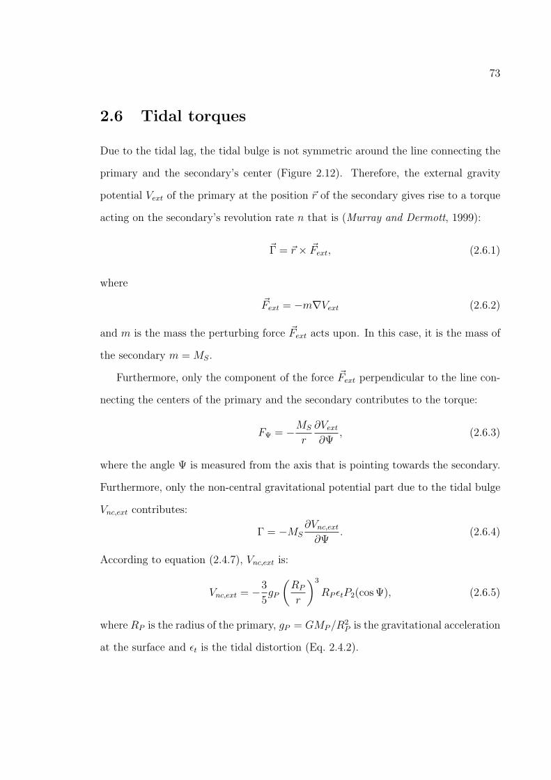
73
2.6 Tidal torques
Due to the tidal lag, the tidal bulge is not symmetric around the line connecting the
primary and the secondary’s center (Figure 2.12). Therefore, the external gravity
potential Vext of the primary at the position r of the secondary gives rise to a torque
acting on the secondary’s revolution rate n that is (Murray and Dermott, 1999):
Γ = r × Fext, (2.6.1)
where
Fext = −m∇Vext (2.6.2)
and m is the mass the perturbing force Fext acts upon. In this case, it is the mass of
the secondary m =MS.
Furthermore, only the component of the force Fext perpendicular to the line con-
necting the centers of the primary and the secondary contributes to the torque:
FΨ = −MS
r
∂Vext∂Ψ
, (2.6.3)
where the angle Ψ is measured from the axis that is pointing towards the secondary.
Furthermore, only the non-central gravitational potential part due to the tidal bulge
Vnc,ext contributes:
Γ = −MS∂Vnc,ext∂Ψ
. (2.6.4)
According to equation (2.4.7), Vnc,ext is:
Vnc,ext = −3
5gP
(RP
r
)3
RP ϵtP2(cosΨ), (2.6.5)
where RP is the radius of the primary, gP = GMP/R2P is the gravitational acceleration
at the surface and ϵt is the tidal distortion (Eq. 2.4.2).

74
In Section 2.4.1, it was shown that the tidal deformation depends on the inner
structure and that the tidal deformation can be described by:
RP ϵt = h2,P ζP , (2.6.6)
where h2,P is a structure constant and ζP = MS/MP (RP/a)3RP is the amplitude
of the equilibrium tide. Inserting into the non-central potential above and setting
k2,P = 3/5 · h2,P yields:
Vnc,ext = −k2,P ζg(RP
r
)3
P2(cosΨ). (2.6.7)
The coefficients k2,P and h2,P were first introduced by A.E.H. Love and are called
’Love numbers’. Murray and Dermott (1999) state that ’They are mostly used as
a convenient way to cloak our ignorance of a body’s internal structure’. If sufficient
information about the inner structure is available, the Love numbers can be calculated
or at least approximated.
If the outer surface of the tidally deformed primary is in hydrostatic equilibrium,
then the total potential is constant at the surface: It is an equipotential plane.
The total potential on the surface is the sum over the central gravity potential at
the deformed surface, the non-central gravity potential with r = RP and the already
known tidal potential at the surface:
−GMP
r− k2,P ζgP2(cosΨ)− ζgP2(cosΨ) = const. (2.6.8)
Substituting r with r = RP (1 + ϵt)P2 cosΨ, the radius of a tidally deformed body,
using a Taylor approximation and setting the sum over all P2(cosΨ)-dependent terms
equal zero to get a constant potential, yields:
k2,P =RP ϵtζ
− 1. (2.6.9)

75
For a two-component model as introduced by Murray and Dermott (1999) and
outlined in section 2.4.1, RP ϵt/ζ = 5/2H and k2,P = 5/2H − 1, where H can range
between 2/5 and 1 (eq. 2.4.14). For a homogenous solid body, on the other hand, are
h2,P = 5/2·1/(1+µ) and k2,P = 3/5h2 = 3/2·1/(1+µ), where µ, the effective rigidity,
is the ratio of gravitational forces over elastic forces determining the tidal deformation.
In any case, for the Love number k2,P the following is true: 0 ≤ k2,P ≤ 3/2.
From this, the torque Γ arising from the primary’s non-central gravity potential
at the position of the secondary (r = a) can be derived:
Γ = −MS∂Vnc,ext∂Ψ
= k2,PGM2
S
a6R5
P
∂P2(cosΨ)
∂Ψ
=3
2k2,P
GM2S
a6R5
P sin(2ϵ)
=3
2k2,P
GM2S
a6R5
P2ϵ (2.6.10)
In the last two steps, two facts are used: Firstly, the tidal bulge is displaced by the
angle ϵ with respect to the line between the centers of masses. Secondly, ϵ is small so
that sin(2ϵ) ≈ 2ϵ, which according to (2.5.10) equals Q−1P , where QP is the primary’s
tidal dissipation factor introduced in the forced damped oscillator framework.
This torque acts at a rate Γn on the secondary and an opposite torque acts at a
rate ΓΩP on the primary, where n is the revolution rate of the secondary and ΩP is
the rotation rate of the primary. This effect is called tidal friction and if ΩP = n,
angular momentum will be transferred between the orbit and the primary’s rotation.
At the same time, the total angular momentum L of the system is conserved i.e.

76
L = 0:
L =d
dt
(CPΩP +
MPMS
Mp +MS
a2n
)= 0, (2.6.11)
where CP = IPMPR2P is the moment of inertia of the rotating primary and the
normalized angular momentum IP reflects the inner mass distribution.
From conservation of angular momentum, the following relation is derived:
CP ΩP = − MPMS
2(MP +MS)naa. (2.6.12)
Therefore, a change in the primary’s rotation results in a change of semi major
axis and the following conclusions can be drawn (Figure 2.12):
• If the primary is rotating faster than the secondary revolves, ΩP > n, the torque
Γ decreases the rotation of the primary at a rate ΓΩP (ΩP < 0). An equal and
opposite torque increases the orbital revolution of the secondary at a rate Γn.
Therefore, the semi major axis a increases (a > 0). This is the case for the
Earth-Moon-system.
• If the primary is rotating slower than the secondary revolves, ΩP < n, the
torque Γ increases the rotation at a rate ΓΩP (ΩP > 0). An equal and opposite
torque decreases the orbital revolution at a rate Γn and the semi major axis
decreases(a < 0). This is the case for the Mars-Phobos-system.
• If the secondary is in a retrograde revolution, the tidal bulge is always lagging
behind the line joining the centers. Therefore, the torque Γ decreases the rota-
tion of the primary at a rate −ΓΩP , therefore ΩP < 0). An equal and opposite
torque decreases the orbital revolution at a rate −Γn, and a < 0. The semi
major axis of the orbit decreases. This is the case in the Neptune-Triton-system.
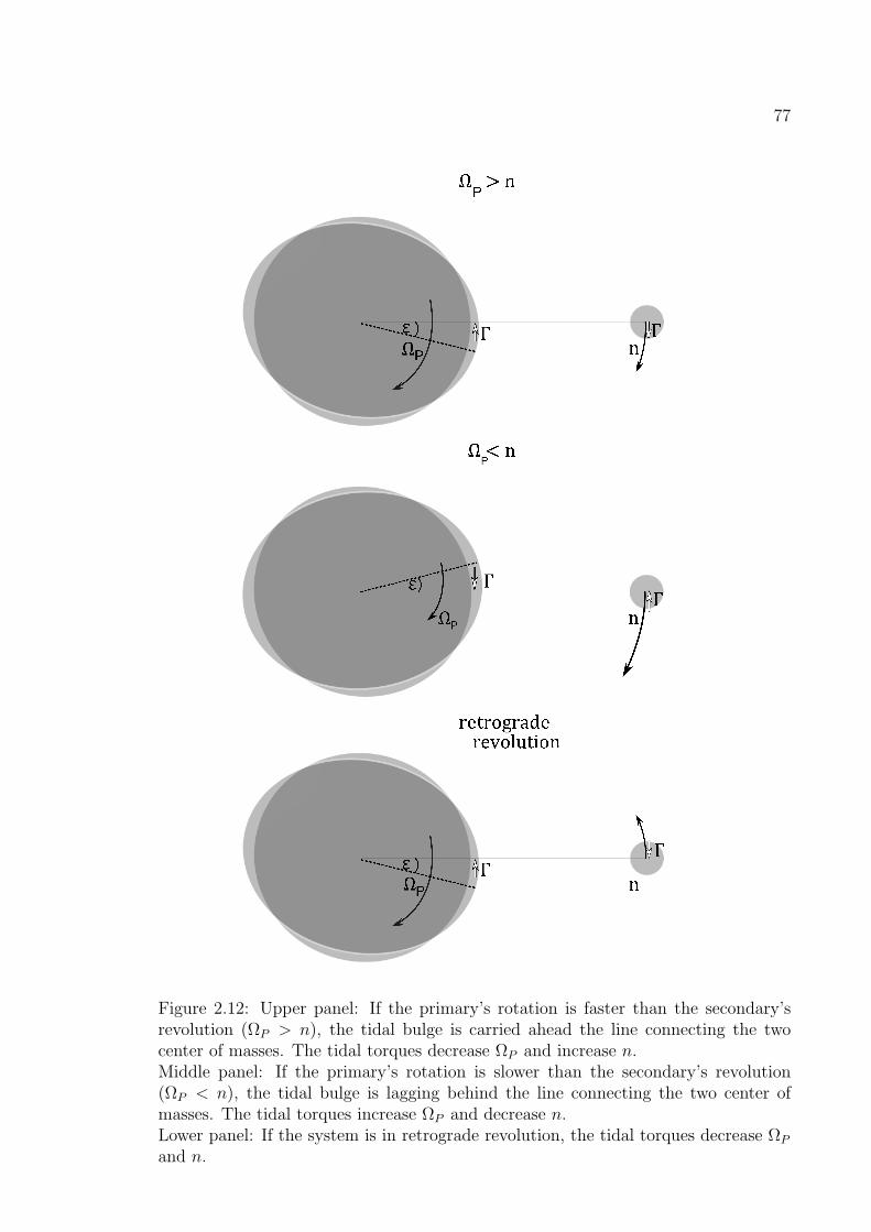
77
Figure 2.12: Upper panel: If the primary’s rotation is faster than the secondary’srevolution (ΩP > n), the tidal bulge is carried ahead the line connecting the twocenter of masses. The tidal torques decrease ΩP and increase n.Middle panel: If the primary’s rotation is slower than the secondary’s revolution(ΩP < n), the tidal bulge is lagging behind the line connecting the two center ofmasses. The tidal torques increase ΩP and decrease n.Lower panel: If the system is in retrograde revolution, the tidal torques decrease ΩP
and n.

78
While the total angular momentum is conserved, if ΩP = n, the total dynamical
energy of the system decreases at a rate:
E = −sign(ΩP − n)Γ(ΩP − n). (2.6.13)
This energy is dissipated within the primary as frictional heat. The rate of energy
dissipation depends on the structure and the energy dissipation mechanisms within.
Murray and Dermott (1999) point out that ’...it is the rate of energy dissipation
that determines the rate of orbital evolution’. Consequently, the orbital evolution is
intricately linked with the inner structure of the primary. It should be noted that the
model described in this Section, keeps the tidal dissipation factor QP constant with
time.
The total dynamical energy of the system affected by the tidal torques is the sum
of the rotational energy of the primary and the orbital energy of the system. The
rate of change of total energy is therefore:
E =d
dt
(1
2CPΩ
2P − GMPMS
2a
)= CPΩP ΩP +
GMPMS
2a2a. (2.6.14)
By inserting Kepler’s third law G(MP + MS) = n2a3, the equation above can be
expressed as:
E = CPΩP ΩP +MPMS
2(MP +MS)n2aa. (2.6.15)
Now equation (2.6.12) is inserted:
E = − MPMS
2(MP +MS)naa(ΩP − n). (2.6.16)
Combined with equations (2.5.10), (2.6.10), (2.6.13), (2.6.16), and Kepler’s third law,
the rate of change in the semi major axis a is derived:
a = sign(ΩP − n)3k2,PMS
QPMP
(RP
a
)5
na. (2.6.17)

79
Inserting equation (2.6.17) into equation (2.6.12) yields the rate of change of angular
velocity:
ΩP = −sign(ΩP − n)3k2,P2IPQP
M2S
MP (MP +MS)
(RP
a
)3
n2. (2.6.18)
Tidal torques due to tides raised by the secondary on the primary are not the
only torques affecting such a system. There are also tidal torques due to tides raised
by the primary on the secondary that need to be considered. These result in angular
momentum transfer between the secondary’s rotation and the orbit and in energy
dissipation within the secondary whose rate is scaled by QS.
The relevant equations describing the semi major axis and secondary’s rotation
evolution are:
aS = sign(ΩS − n)3k2,SMP
MS
(RS
a
)5
na (2.6.19)
ΩS = −sign(ΩS − n)3k2,S2ISQS
M2P
MS(MP +MS)
(RS
a
)3
n2. (2.6.20)
Therefore, the complete tidal evolution of the system due to the displacement of the
tidal bulges on the primary and the secondary from the line connecting the centers of
masses can be found by adding equations (2.6.19, 2.6.17) and combining them with
(2.6.20) and (2.6.18). In the next chapter, however, it will be found that for most
planetary systems discovered in this work, ΩS ≈ n is a good assumption. Therefore,
aS ≈ 0 and ΩS ≈ 0.
As a consequence, the long-term evolution of the semi major axis can be calculated
by integrating Eq. (2.6.17) at first order. This yields for evolution in the past:
2
13a13/20
[1−
(aia0
)13/2]= sign (ΩP − n)
3k2,PQP
(G
MP
)1/2
R5PMS∆tpast (2.6.21)

80
where ai is the initial, a0 is the current semi major axis and ∆tpast > 0 is the elapsed
time; assuming that the orbit was approximately circular during ∆tpast, that MS ≪
MP and that either ΩP > n or ΩP < n during the whole integration time.
For evolution in the future this yields:
2
13a13/20
[(aea0
)13/2
− 1
]= sign (ΩP − n)
3k2,PQP
(G
MP
)1/2
R5PMS∆tfuture, (2.6.22)
where a0 is the current, ae is the future semi major axis and ∆tfuture is the time
needed to achieve the future position. This relation is used in this work to estimate
tidal evolution time scales for circular orbits (Section 4.1 and Section 8.4.2).
2.7 Tidal evolution of eccentric orbits
Up to now, the orbit was assumed to be circular which is a good approximation for
many planets and moons in our Solar System. In the past years, extrasolar planets
on short-period orbits with large eccentricities were found. The orbit of CoRoT-10b,
for example, has e = 0.5. Therefore, the equations derived in the previous section
for circular orbits no longer hold. Hut (1981) calculates the force arising due to the
non-central gravity potential of the tidal bulge for a secondary on an eccentric orbit
using a different derivation than the one in the previous section following Murray and
Dermott (1999). Hut (1981) calculates the perturbed gravitational force between the
primary and the secondary due to two point masses at the surface of the primary
which represent the two tidal bulges. For e = 0, the tidal torques derived by Murray
and Dermott (1999) and Hut (1981) are the same. This will be shown by comparing
the Ψ-component of the force acting perpendicular to the line connecting the centers
of masses which is the only relevant force-component when the orbit is circular.
81
Hut (1981) derives:
FΨ = 3GM2
S
r2
(RP
r
)5
k2,P τP
(ΩP − Ψ
), (2.7.1)
where Ψ is the instantaneous revolution rate, Ψ is the true anomaly of the orbit, τP
is a small time lag for the tidal bulge to form on the primary. Furthermore, r is
the distance between the primary’s and secondary’s center of mass, which can vary
between a(1 ± e) for eccentric orbits, k2,P is the Love number2. FΨ creates a torque
Γ = rFΨ on the secondary.
Comparing this torque Γ with the torque calculated in the previous section shows
that the equations (2.6.10) and (2.7.1) are equal for e = 0, r = a, and Ψ = n. For a
circular orbit
τP (ΩP − n) = ϵ, (2.7.2)
where ϵ is again the tidal lag angle introduced in the forced oscillator framework,
2|ϵ| = Q−1P (see eq. (2.5.10)). If the system is not close to resonance and weakly
damped, i.e., if the damping time scale τd is large, then equation (2.5.7) holds:
Q−1P =
|ω|/τdω20
, (2.7.3)
where ω0 is the resonance frequency which is a constant property of the primary
and ω = 2|ΩP − n| is the frequency of the tidal waves. Consequently, the time lag
τP = 1/(τdω20) is indeed small and constant as required by Hut (1981). τP and QP
are connected for circular orbits via the following relation:
Q−1P = 2|ΩP − n|τP . (2.7.4)
2Hut (1981) calls k2,P the apsidal motion constant.

82
This relation describes one factor that causes much confusion when comparing liter-
ature on tidal interactions from the planetary science and the astronomy community.
Whereas the first group often uses the tidal dissipation QP to quantify the strength
of tidal friction and keeps this parameter constant over time, the latter group often
uses the time lag τP to quantify the strength of tidal friction and keeps this parameter
constant over time. As long as ΩP −n ≈ const, both approaches yield similar results.
Care has to be taken when ΩP − n is not constant over time. This will be discussed
in more detail in subsequent chapters when applying the relevant equations.
The effect of the force component FΨ on the orbital parameters for the general
case of eccentric orbits can be found by calculating the energy loss during one orbit
under conservation of angular momentum. The sum of orbital angular momentum
Lorb and rotational angular momentum of the primary Lrot,P needs to be conserved
under force FΨ, where the orbital angular momentum is:
Lorb =MPMS
MP +MS
na2√1− e2, (2.7.5)
and the rotational angular momentum is:
Lrot,P = IPMPR2PΩP . (2.7.6)
The rate of change in orbital angular momentum is:
Lorb =1
2
MPMS
MP +MS
naa√1− e2 − MPMS
MP +MS
na2ee√1− e2
. (2.7.7)
The orbital energy is
Eorb = −GMPMS
2a, (2.7.8)
and its rate of change is:
Eorb =d
dt
(−GMPMS
2a
)= G
MPMS
2a2a. (2.7.9)

83
The angular momentum of a barycentric orbit is connected to the position vector r
and the mean anomaly Ψ by
Lorb =MPMS
MP +MS
h, (2.7.10)
where the constant h is
h = r2Ψ, (2.7.11)
and the position vector r in polar coordinates is:
r = a1− e2
1 + e cosΨ. (2.7.12)
As was already stated, FΨ creates a torque Γ = rFΨ on the secondary by the tides
raised on the primary. The corresponding orbital energy loss is:
∆EΨ =
∫ 2π
0
ΓdΨ = 3GM2SR
5Pk2,P τP
∫ 2π
0
ΩP − Ψ
r6dΨ. (2.7.13)
Using the equations (2.7.5),(2.7.10), (2.7.12), integrating over Ψ, inserting the mean
motion n =√G(MP +MS)a
−3/2 and dividing by the orbital period Porb – which
according to Kepler’s third law is (Porb = 2πa3/2/√G(MP +MS)) – gives
EΨ = −3k2,PTP
G(MP +MS)M2
S
MP
(RP
a
)8(1− e2)−15/2
af2(e), (2.7.14)
where TP is the typical tidal time scale defined by Hut (1981) as TP =R3
P
GMP τPand
f2(e) is a function depending on e:
f2(e) =
(1 + 14e2 +
105
4e4 +
35
4e6 +
35
128e8)
(2.7.15)
− ΩP
n(1− e2)3/2
(1 +
15
2e2 +
45
8e4 +
5
16e6).
The corresponding change in semi major axis due to the loss of orbital energy is
derived by using (2.7.9) and solving for a:
a = −6k2,PTP
q(1 + q)
(RP
a
)8
a(1− e2)−15/2f2(e), (2.7.16)

84
where the mass ratio q =MS/MP is introduced.
The amount of orbital angular momentum transferred to the primary’s rotation
per orbit is calculated by:
∆Lorb =
∫orbit
Γdt =
∫ 2π
0
ΓdΨ
Ψ. (2.7.17)
It follows by integrating over Ψ and dividing by Porb:
dLorb
dt= −3
k2,PT
√G(MP +MS)
M2S
MP
R8Pa
−15/2(1− e2)−6f3(e) (2.7.18)
with
f3(e) =
(1 +
15
2e2 +
45
8e4 +
5
16e6)− ΩP
n(1− e2)3/2
(1 + 3e2 +
3
8e4). (2.7.19)
The change in eccentricity e is derived by using equation (2.7.7) and inserting a and
Lorb as determined above:
e = −3
2
k2,PTP
q(1 + q)
(RP
a
)8
(1− e2)−13/2ef4(e), (2.7.20)
with
f4(e) =
(15 +
225
4e2 +
225
8e4 +
75
64e6)
(2.7.21)
− ΩP
n(1− e2)3/2
(11 +
33
2e2 +
11
8e4).
Lorb is transferred to the primary. The angular momentum of the primary is IPMPR2PΩP .
IP is the normalized moment of inertia. Therefore, the angular momentum transfer
results in a change of the primary’s rotation rate ΩP which is derived by setting
(2.7.18) equal to
dLorb
dt= IPMPR
2P
dΩP
dt(2.7.22)

85
and solving for ΩP . This yields
ΩP = 3k2,PT
q2
IP
(RP
a
)6
(1− e2)−6nf3(e). (2.7.23)
In addition to FΨ, a radial force component arises due to the non-central gravity
potential when the orbit is eccentric. The distance r between the primary and the
secondary is not constant anymore.
As a reminder, the potential is (eq. 2.6.7):
Vnc,ext(r(t)) = −k2,P ζPgP(
RP
r(t− τP )
)3
P2(cosΨ), (2.7.24)
where k2,P is the Love number, gP and ζP are the surface gravity acceleration and the
amplitude of the equilibrium tide on the primary. The tidal potential of the secondary
acted at a time t−τP to form the tidal bulge, where τP is the tidal time lag, when the
secondary was at a distance r(t− τP ). At time t, when the displacement of the tidal
bulge gives rise to a force acting on the secondary, this secondary is at distance r(t).
The distance r(t− τP ) with respect to r(t) is r(t− τP ) ≈ r(t)− rτP = r(t)(1− rrτP ).
Inserting this into the potential and using Taylor approximation yields:
Vnc,ext(r) = −k2,P ζPgP(
RP
r(1− rrτP )
)3
P2(cosΨ)
≈ −k2ζPgP(RP
r
)3
(1 + 3r
rτP )P2(cosΨ). (2.7.25)
Note that ζP , the amplitude of the equilibrium tidal bulge at the time of the tidal
bulge formation due to the tidal potential of the secondary, is constant in this context.
It does not change when the tidal bulge is displaced with respect to the line connecting
the centers of masses. This is equivalent to stating that the height of the tidal bulge
does not change between t − τP and t. Therefore, the radial force component Fr

86
due to the displacement of the tidal bulge acting on the secondary at distance r(t) is
derived from:
Fr = −MS∂Vnc,ext(r)
∂r
≈ −3k2,PMSζPgP
(RP
r
)3 (1 + 3 rrτP )
r
= −3k2,PGM2
S
r2
(RP
r
)5
(1 + 3r
rτP ), (2.7.26)
where the boundary condition Ψ(t) = ϵ was used. P2(cos ϵ) ≈ 1 because the tidal lag
angle is small: ϵ ≪ 1. In the last step ζP = MS
MP
(RP
r
)3and gP = GMP
R2P
were inserted.
While ζP was constant during the tidal lag time τP , it is not constant over the whole
orbit when this orbit is eccentric. ζP varies over time because the tidal force of the
secondary, that forms the tidal bulge, varies over one orbit as the distance r between
the primary and secondary alternatively grows and shrinks.
The corresponding energy loss ∆E due to the radial force Fr is computed by:
∆Eradial =
∫orbit
Frdr =
∫ 2π
0
Frdr
dΨdΨ. (2.7.27)
The radial force does not change the orbital angular momentum and therefore Lorb =
0. (Note that for a circular orbit drdΨ
= 0 and ∆Eradial = 0.) Using the equations
(2.7.5), (2.7.10), (2.7.12) and integrating over Ψ yields:
∆Eradial = −9πG3/2(MP +MS)1/2M2
SR5Pk2,P τPa
−15/2(1− e2)−15/2f(e), (2.7.28)
where f(e) is:
f(e) = e2[1 +
15
4e2 +
15
8e4 +
5
64e6]. (2.7.29)
∆Eradial is negative as expected for a dissipative process. To derive the mean orbital
energy loss Eorb, ∆Eradial is divided by the orbital period P .

87
Consequently, Eradial is:
Eradial = −9
2G2(MP +MS)M
2SR
5Pk2,P τPa
−9(1− e2)−15/2f(e). (2.7.30)
The change in the semi major axis a as a consequence of Fr acting on the orbit is
derived by setting Eradial = Eorb (equation 2.7.9) and solving for a:
a = −9k2,PTP
q(1 + q)
(RP
a
)8
a(1− e2)−15/2f(e). (2.7.31)
The change in eccentricity e is derived by using the relation (2.7.5) and Lorb = 0
(2.7.7) and solving for e:
e = −9
2
k
Tq(1 + q)
(R
a
)8
(1− e2)−13/2f(e)
e. (2.7.32)
The total change in the semi major axis a and eccentricity e due to Fr and FΨ is
derived by adding (2.7.31) to (2.7.16) and adding (2.7.32) to (2.7.20).
This results in the following set of equations for the tidal evolution of the system
due to the lag of the tidal bulge on the primary:
aP = −6k2,PTP
q(1 + q)
(RP
a
)8
an−1(1− e2)−15/2[nf1(e)− (1− e2)3/2f2(e)ΩP
](2.7.33)
eP = −27k2,PTP
q(1 + q)
(RP
a
)8
en−1(1− e2)−13/2
[nf3(e)−
11
8(1− e2)3/2f4(e)ΩP
](2.7.34)
and
ΩP = −3k2,PTP
q2
IP
(RP
a
)6
(1− e2)−6[nf2(e)− (1− e2)−3/2f5ΩP
], (2.7.35)
88
where
f1(e) = 1 +31
2e2 +
225
8e4 +
185
16e6 +
25
64e8
f2(e) = 1 +15
2e2 +
45
8e4 +
5
16e6
f3(e) = 1 +15
4e2 +
15
8e4 +
5
64e6 (2.7.36)
f4(e) = 1 +3
2e2 +
1
8e4
f5(e) = 1 + 3e2 +3
8e4.
Up to now, tidal evolution due to tides raised by the secondary on the primary
was calculated. As was stated in the previous section, the tidal evolution due to
tides raised by the primary on the secondary needs to be taken into account as well.
This results in a set of equation similar to the ones above safe for the fact that the
subscripts P and S are exchanged and q =MS/MP needs to be replaced by 1/q. The
complete tidal friction evolution is described by adding aP and aS and eP and eS and
complementing them with the equations describing the evolution of the primary’s and
secondary’s rotation evolution ΩP and ΩS.
The equations used in this section use the typical tidal time scale TP which con-
tains the tidal lag time τP to determine the rate of change of the orbital elements.
This quantity is defined as:
TP =R3
P
GMP τP. (2.7.37)
This is connected to the tidal dissipation factor QP by:
τP =1
2QP |ΩP − n|. (2.7.38)
Therefore, inserting into the equations above
TP =2R3
PQP |ΩP − Ψ|GMP
(2.7.39)

89
yields equations dependent on QP which are used by other authors (see the next
Section).
The difference between a tidal friction model parameterized with QP
k2,Pand a model
parameterized with τP will be discussed in more detail in subsequent chapters.
2.8 The tidal dissipation factor and the Love num-
ber
In the previous sections, the importance of the tidal dissipation factor Q and the Love
number k2 for describing tidal friction became apparent. The quantity Q describes
the energy loss of a damped externally driven oscillator. Q is inversely proportional
to the amount of energy dissipated per cycle (see section 2.5, equation (2.5.6)). The
larger Q, the less energy is dissipated, the smaller Q the more energy is dissipated.
The Love number k2, on the other hand, describes the feedback effect on the tidal
deformation due to the self-gravity on the tidal bulge. If k2 = 0, there is no feedback
effect and the tidal deformation has the same amplitude as the tidal equilibrium tide
ζ. If k2 = 1.5, the feedback effect is maximal and the tidal deformation is 2.5 times
as large as ζ (see Section 2.4.1). Both quantities are dimensionless parameters that
contain the knowledge (or lack thereof) of the processes that are at work within a
celestial body that is deformed and excited by tides.
Furthermore, the parameter Q/k2 determines the secular change of the semi ma-
jor axis and rotation rates, so a good constraint on Q/k2 is critical for successful
predictions of the dynamical evolution of planetary systems. The argument can also
be reversed. If Q and k2 are constrained, this may help to improve our understanding
90
of inner processes of the tidally excited body.
Historically, Q/k2 was first investigated for the Earth-Moon system. With the
advent of the space age, attempts were made to constrain Q/k2 in the Solar System
and this was used to gain knowledge on the inner structure of bodies different from
the Earth and the Moon, even when in-situ measurements are not possible. Selected
publications will be discussed in the following to gain insight about the possible
magnitude of Q/k2 and the timescales on which dynamical evolution due to tidal
friction takes place.
Furthermore, it will be shown that for the stellar tidal dissipation factor Q∗k2,∗
, there
are large uncertainties that cover several orders of magnitude. Indeed, these uncer-
tainties provide one of the the main motivations for this work which puts constraints
on Q∗k2,∗
and explains why different approaches yield different Q∗k2,∗
-values.
It should be noted that in many works discussed in this section, Q/k2 is regarded
as approximately constant over time. This basic assumption and its limitations will
be discussed in more details in the next Chapter, in Section 3.1.
2.8.1 Q/k2 in the Solar System
Earth and Moon
Already Thomson (1863a) derived k2,Earth = 0.36 from measuring the solid body tide
of the Earth. From this and the Lunar Laser ranging (LLR) measurements, the tidal
dissipation factor Q of the Earth can be deduced. LLR measurements determined the
rate at which the Moon’s semi major axis increases to be: a = 3.74 cm/yr (Murray
and Dermott, 1999; Lambeck, 1977). Inserting a into equation (2.6.17), the current

91
ratio of tidal dissipation factor over Love number is derived:
QEarth, current
k2,Earth, current≈ 12.
For the tidal dissipation factor and Love number of the Moon, the following parame-
ters were derived based on measurements from the Apollo seismic network (Lambeck,
1977):
QMoon ≈ 300 for the central region,
QMoon ≈ 1000 for the upper 500− 600 km,
k2,Moon ≈ 0.02. (2.8.1)
Mars
Pollack (1977) estimates QM
k2,M≈ 100 based on the measured secular decrease of the
semi major axis of Phobos (Born and Duxbury, 1975; Shor, 1975) due to tidal friction
because of tides raised by Phobos on Mars. This work was revised by Lainey et al.
(2007) who derived:
QMars = 79.9± 0.7
k2,Mars = 0.152,
based on the measured decay rate of Phobos’ semi major axis (20 cm/yr) taken from
observations between 1877 and 2005 and spacecraft observations from Mars Express
and Mars Global Surveyor.
For the Mars moon Phobos, Lambeck (1979) derived:
QPhobos ≈1
5QMars
k2,Phobos = 10−4, (2.8.2)

92
assuming that Phobos was captured by Mars about four billion years ago and that
the initially high eccentricity that such captured asteroids usually show was damped
by tidal friction.
Jupiter, Saturn and Uranus
Starting in the 60s of the last century, several authors estimated QJupiter and QSaturn
based on the fact that many of the satellites of these gas giants are in orbit resonances.
Most notably, the mean motions of the Galilean moons Io, Europa and Ganymede (n1,
n2 and n3, respectively) obey the following relation: n1−3n2+2n3 = 0. Furthermore,
the saturnian satellites Enceladus and Dione as well as Mimas and Thethys each form
a pair with mean motion resonances. Assuming that the satellites have evolved into
this state due to tidal friction and are now stable, the time averaged Q was estimated
by Goldreich (1965) to be:
QJupiter ≈ (1− 2)× 105
QSaturn ≈ (6− 7)× 104.
k2, on the other hand, was assumed as
k2 =3
2
(1 +
19µ
2gρRP
)−1
≈ 1, (2.8.3)
where g, ρ, µ, and RP are the surface gravity, density, rigidity and radius of the gas
giants, respectively (See Section 2.4.1).
In 1977, Goldreich and Nicholson (1977) contradicted Goldreich (1965) by stating
that if turbulent viscosity in the atmosphere of Jupiter is the dominant mechanism
by which energy is dissipated then QJupiter ≈ 5×10¹³. This would mean that no tidal
evolution of the Galilean moons could have occurred and that the amount of energy

93
dissipated within Jupiter is negligible. Note the difference in Q by eight orders of
magnitude. Dermott (1979b) on the other hand states that energy dissipation in the
solid or quasi-solid core of gas giants is important (Qe ≈ 60 in the core). The total
averaged Q for Jupiter and Saturn can then be in the orders of 105 and allow for the
tidal evolution of the inner Jupiter and Saturn satellites; but only if it is assumed
that the dense cores of Jupiter and and Uranus have volumes twice as large as that
of the Earth. For Saturn, a dense core of eight times the Earth’s volume is required.
Today, it is still uncertain if Jupiter has a dense core and how large it is (Saumon
and Guillot, 2004). A dense core, however, is postulated for the core-instability or
core-accretion mechanism that explains the formation of gas giants (Pollack et al.,
1986; Wuchterl, 1993). Furthermore, a number of extrasolar gas giants have been
discovered that confirm this scenario. The planet HD 149026, for example, probably
has a 67 Earth mass core (Sato et al., 2005).
Later investigations derived tidal dissipation factors in the orders of 104 − 105 for
Solar System gas giants and not in the orders of 1013: In 1990, Tittemore and Wisdom
(1990) constrained Q for Uranus by investigating the tidal evolution of Miranda,
Umbriel and Ariel and derived 1.1× 10⁴ ≤ QUranus ≤ 3.9× 10⁴.
Only recently, Lainey et al. (2009) derived the following values for Jupiter and Io
from astrometric observations:
k2,IoQIo
= 0.015± 0.003
k2,JupQJup
= (1.102± 0.023)× 10−5.
Leconte et al. (2011) derived k2 based on numerical models and compared them with

94
observations. They give for Jupiter and Saturn planets:
k2,Jup ≈ 0.5 (2.8.4)
k2,Sat ≈ 0.3. (2.8.5)
A comparison of the different QP
k2,Pvalues within the Solar System allows to draw
the following conclusion: rocky planets and moons apparently have QP
k2,P≈ 10 − 100
and gas giants have QP
k2,P≈ 104 − 105. Therefore, rigid bodies are much more efficient
in dissipating tidal energy than gaseous bodies, as expected intuitively. Furthermore,
for very small rocky bodies like the Moon and Phobos the Love number is very small.
There is almost no feedback effect due to the self-gravity of the tidal bulge. In
contrast to that, the Earth, Jupiter and Saturn allow for moderate feedback effects.
k2,Jup ≈ 0.5 , for example, means that the tidal deformation is 1.5 times the amplitude
of the tidal equilibrium tide ζJup.
2.8.2 Q/k2 in extrasolar planet systems
Q/k2 for brown dwarfs
Heller et al. (2010) constrain QP for brown dwarfs by:
QP > 104.5 (2.8.6)
to allow the eclipsing brown dwarf binary 2MASSJ05352184-0546085 to become
synchronized. The Love number for brown dwarfs is assumed as k2 = 0.286. The
Love number and tidal dissipation factor found by Heller et al. (2010) agree with the
Love number and tidal dissipation factor found for gas giants. This would mean that

95
brown dwarfs dissipate tidal energy and are tidally deformed like gas giants and not
like main sequence stars.
Q∗k2,∗
for main sequence stars
Leconte et al. (2011) give the following simple equation to derive the Love number
k2,∗:
k2,∗ =3
2
(I∗5
2
)2 (1− n
5
), (2.8.7)
where I∗ is the normalized moment of inertia and n is the polytropic index used for
the modeling of the inner stellar density and pressure by the Lane-Emden equation
(for example Prialnik (2000)). It is beyond the scope of this work to describe stellar
models in detail. It shall be sufficient to state that for main sequence stars, n ≈ 3 is
used and the normalized moment inertia is assumed as I∗ = 0.074 (See Section 2.11).
From this, the stellar Love number is derived:
k2,∗ = 0.018. (2.8.8)
Hut (1981) gives k2,∗ ≈ 0.01 which agrees within order of magnitude.
Therefore, when comparing tidal interaction models in the literature one has to
check if Q∗k2,∗
or Q∗ is discussed, because both values may differ by a factor of 50 just
due to the Love number. Throughout this work, k2,∗ = 0.018 is assumed. This small
number indicates that almost no feedback occurs due to the self-gravity of the tidal
bulge in contrast to planets like Earth or Jupiter. The tidal deformation is almost
identical to the equilibrium tide indicating that main sequence stars behave in that
respect like a rigid sphere covered by a zero-density fluid (Section 2.4.1).
In the following, several Q∗k2,∗
values are discussed derived in the last two decades.
In 1996, shortly after the discovery of the first extrasolar planets, Rasio et al. (1996)

96
calculated wether jovian planets like 51 Pegasi b could be stable under tidal friction.
It was assumed that the star is a slowly rotating main-sequence star like our Sun
(PSun ≈ 27 days) and that the planet has a circular orbit with a short revolution
period of a few days. In such a case, the stellar rotation rate is smaller than the
revolution rate (Ω∗ < n) and consequently the application of (2.6.17) or (2.7.33) for
e = 0 yields a decrease of the planet’s semi major axis. (In the following, the star
is regarded as the primary whose parameters are denoted by subscript ∗, whereas
Pl denotes planetary parameters. The planet is the secondary in the tidal friction
context.).
The authors estimated the orbital decay rate τa assuming that the tidal energy is
entirely dissipated within the convective envelope by viscous dissipation:
1
τa=
|a|a
=f
τc
Menv
M∗
q
1 + q
(R∗
a
)8
, (2.8.9)
where M∗ and R∗ are the radius of the host star, a is the distance between the star
and the extrasolar planet, q is the ratio of planetary mass to stellar mass, Menv is the
mass of the convective outer layer in the main sequence star, τc is the eddy turnover
time scale and f is a numerical value found by integrating viscous dissipation of tidal
energy over the convective envelope. Comparing this equation with (2.7.33), it is
obvious that the equations are very similar and can be related to each other to derive
the corresponding tidal dissipation factor of the star Q∗k2,∗
.
f
τc
Menv
M∗=
6k2,∗T∗
Ω∗ − n
n
=3k2,∗GM∗
Q∗R3∗n
with n =√G(M∗ +MPl)/a3, where MPl is the mass of the exoplanet, and
T∗ = R3∗Q∗2(Ω∗ − n)/(GM∗). Rasio et al. (1996) further derived τa ≈ 4 × 10⁴ Gyrs

97
for a solar-like slowly rotating star (M∗ = MSun, R∗ = RSun, Menv/MSun = 0.028,
Ω∗ << n) and an extrasolar planet with mass MPl = 10−3MSun and semi major axis
a = 11, RSun = 0.511 AU. This corresponds to
Q∗
k2,∗≈ 4× 10⁸ (2.8.10)
or
Q∗ = 8× 10⁶. (2.8.11)
This is more than one order of magnitude higher than the QPl-values of the gas giants
in the Solar system. This would indicate that if stars dissipate energy by turbulent
viscosity in their convective envelope, they are even less efficient in dissipating tidal
energy than gas giants who also contain a turbulent atmosphere. This is compatible
with the discussion of QPl
k2,P lof gas giants in the 1970s, when it was found that turbulent
viscosity is not an efficient energy dissipation mechanism. Instead, additional energy
dissipation in dense cores had to be inferred to account for the observed QPl
k2,P lvalues.
On the other hand, such a large Q∗k2,∗
would mean that the planet is safe from orbital
decay within the lifetime of the star; which is about 10 Gyrs for a main sequence star
- much less than the decay time.
Recently, Penev and Sasselov (2011) derived Q∗k2,∗
values of
Q∗
k2,∗= 108 − 3× 10⁹, (2.8.12)
based on numerical simulation of tidal energy dissipation in externally-perturbed con-
vective volumes. Their work was stimulated by the fact ”(...)that a comprehensive
theoretical understanding of turbulent dissipation in stellar convection zones is lack-
ing.” These values agree nicely with the one given by Rasio et al. (1996) and also the

98
one derived by Carone and Patzold (2007): 3× 10⁷ ≤ Q∗k2,∗
≤ 2× 10⁹ and Patzold and
Rauer (2002): Q∗k2,∗
≥ 1.5× 10⁸.
These values are, however, much higher than those used by many other authors
(Jackson et al. (2008) Q∗k2,∗
= 105.5, Dobbs-Dixon et al. (2004) Q∗k2,∗
= 105 − 106, and
Lin et al. (1996), Q∗k2,∗
= 105). In summary, all given values cover the following range:
Q∗
k2,∗= 105 − 3× 10⁹, (2.8.13)
which would correspond to
Q∗ = 2× 10³ − 6× 10⁷, (2.8.14)
The lower values are derived from synchronization time scales of main sequence
stellar binaries (Meibom and Mathieu, 2005).
This work aims to constrain Q∗k2,∗
by applying tidal friction models to extrasolar
planets and discussing their dynamical evolution. Indeed, it will be shown that Penev
and Sasselov (2011)’s work will become particularly important when discussing the
Q∗k2,∗
-constraints derived in this work. In any case, the variety of possible Q∗k2,∗
-values
presented here shows how important it is to derive improved constraints on the stellar
dissipation factor. Otherwise, it is almost impossible to predict the orbital evolution
of a close-in extrasolar planet.
2.9 Stability of tidal equilibrium
If the orbit of a tide raising body is circular and ΩP = ΩS = n, then in principle no
tidal friction can occur and the orbital elements will remain unchanged as long as
no other mechanism removes angular momentum from the system. It will be proven
that such a configuration can be achieved only under certain constraints.

99
Hut (1980) investigates the stability of such a state for a system of two celestial
bodies which exchange significant tidal forces. The state of such a binary system is
considered from the viewpoint of the barycentric orbit. Although Hut (1980) devel-
opes this formalism for stellar binary systems, the same method can be applied to a
’binary systems’ composed of a star and a planetary companion. The binary system
is determined in the most general case by the semi major axis a of the orbit and its
eccentricity e, the angle i between the orbital angular momentum Lorb and the total
angular momentum Ltot and the rotation rates ΩP and ΩS of the primary and the
secondary (Figure 2.13) before it enters a double synchronous state.
Figure 2.13: The barycentric orbit configuration of a binary system including itsrelevant parameters. L is the total angular momentum Ltot and h is the orbitalangular momentum Lorb (Hut, 1980).
The total angular momentum Ltot is composed of the orbital angular momentum

100
and the rotation angular momenta:
Ltot =MPMS
MP +MS
na2√1− e2 + IPMPR
2P ΩP + ISMSR
2SΩS, (2.9.1)
where IP and IS are the normalized moments of inertia of the primary and secondary
with masses MP and MS and radii RP and RS, respectively, and n is the orbital
revolution rate or orbital mean motion.
The total energy Etot is composed of the orbital energy and the rotational energy
of each body:
Etot = −GMPMS
2a+
1
2IPMPR
2P
∣∣∣ΩP
∣∣∣2 + ISMSR2S
∣∣∣ΩS
∣∣∣2 . (2.9.2)
A system is considered stable if its energy is minimal. In addition, the angular
momentum needs to be conserved (dLtot
dt= 0). A good way to solve this problem is
the application of Lagrange multipliers, a mathematical method to find maxima and
minima of a function subject to additional constraints.
For this example, the application of the Lagrange multipliers yields:
0 =∂
∂xiE + λx
∂
∂xiLtot,x + λy
∂
∂xiLtot,y + λz
∂
∂xiLtot,z (2.9.3)
where xi are the nine free parameters that describe the system
a, e, i,ΩP,x,ΩP,y,ΩP,z,ΩS,x,ΩS,y, and ΩS,z and the Lagrange multiplicator λ is a con-
stant vector.
Hut (1980) expresses the equations above in units of length (IPMPR2P )
1/2M−1/2P ,
units of time G−1/2M−5/4P (IPMPR
2P )
3/4 and units of mass MP . In that case, MP ,
IPMPR2P , and G can be set to one. In addition, a coordinate system was chosen
where the z-axis is oriented along the vector Ltot = (0, 0, |Ltot|)) and where Lorb =
(|Lorb| sin i, 0, |Lorb| cos i) is in the (x, z)-plane.

101
The equations of total energy and total angular momentum reduce to:
Etot = − q
2a+
1
2
(Ω2
P,x + Ω2P,y + Ω2
P,z
)+
1
2γ(Ω2
S,x + Ω2S,y + Ω2
S,z
)(2.9.4)
and
Ltot,x = 0 = |Lorb| sin i+ ΩP,x + γΩS,x (2.9.5)
Ltot,y = 0 = ΩP,y + γΩS,y
Ltot,z = |Ltot| = |Lorb| cos i+ ΩP,z + γΩS,z,
where q is the ratio of the masses q = MS/MP and γ is the ratio of the moments of
inertia γ = ISMSR2S/IPMPR
2P . Equations (2.9.5) now yield:
0 =q
a+ λx|Lorb| sin i+ λz|Lorb| cos i (2.9.6)
0 =e
1− e2|Lorb| (λx sin i+ λz cos i)
0 =λx cos i− λz sin i
0 =ΩP,i + λi (i = x, y, z)
0 =ΩS,i + λi (i = x, y, z).

102
The conditions above are met when:
ΩP,z =n (2.9.7)
ΩS,z =n
e =0
i =0
ΩP,x =0
ΩP,y =0
ΩS,x =0
ΩS,y =0,
where n =√
1+qa3
is the orbital revolution rate.
Therefore, the system is in equilibrium when the orbit is circular, all rotation
vectors are parallel to each other and all rotation rates are equal (ΩP,z = ΩS,z = n).
This is called a double synchronous state state.
The total angular momentum Ltot,doub of a system in double synchronous state is
Ltot,doub =q
(1 + q)1/3n−1/3 + (1 + γ)n. (2.9.8)
Figure 2.14 shows the possible Ltot,doub-values with respect to n. A double syn-
chronous equilibrium state is only possible if Ltot,doub is greater than the critical an-
gular momentum Ltot,crit. Ltot,crit can be found with (2.9.8) by solvingdLtot,doub
dn= 0
for n. In modified units of time, mass and length this yields:
Ltot,crit = 4
[1
27(1 + γ)
q3
1 + q
]1/4(2.9.9)
or
Ltot,crit = 4
[G2
27
(IPMPR
2P + ISMSR
2S
) M3PM
3S
MP +MS
]1/4(2.9.10)

103
in SI-units.
For Ltot = Ltot,crit, the following holds for the individual components of the total
angular momentum:
Lorb,crit =3(1 + γ)ncrit (2.9.11)
Lrot,crit =ΩP + γΩS = (1 + γ)ncrit,
with ncrit:
ncrit =1
33/4
((1 + γ)3
√1 + q
q
)−3/4
. (2.9.12)
In other words, a stable double synchronous state only exists if the orbital angu-
lar momentum is at least three times larger than the sum of the angular momenta
contained in the rotation of the two individual bodies. Therefore, Lorb has to exceed
the following critical value to allow for a stable double synchronous rotation state:
Lorb > Lorb,crit = 3 (1 + γ)ncrit (2.9.13)
in modified units and
Lorb > Lorb,crit = 3(IPMPR
2P + ISMSR
2S
)ncrit (2.9.14)
in SI-units.
As can be seen in Figure 2.14, there exist two possible states where the rotation
rates can be synchronized if Ltot > Ltot,crit. But only the state with the wider orbit i.e.
the smaller n is stable, because here the total energy is minimal as well, whereas for
the orbit with the larger n, the total energy is maximal. For n = ncrit only one solution
exists with Ltot = Ltot,crit, which is unstable because in that case Lorb = Lorb,crit, as
well. And it was found previously that only orbits with Lorb > Lorb,crit can establish
a stable double synchronous state.
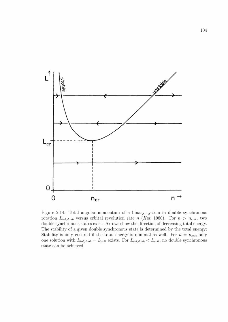
104
Figure 2.14: Total angular momentum of a binary system in double synchronousrotation Ltot,doub versus orbital revolution rate n (Hut, 1980). For n > ncrit, twodouble synchronous states exist. Arrows show the direction of decreasing total energy.The stability of a given double synchronous state is determined by the total energy:Stability is only ensured if the total energy is minimal as well. For n = ncrit onlyone solution with Ltot,doub = Lcrit exists. For Ltot,doub < Lcrit, no double synchronousstate can be achieved.

105
2.10 Evolution of the rotation of main sequence
stars
To investigate tidal interactions between close-in extrasolar planets and their host
stars, the evolution of the stellar rotation of main sequence stars needs to be included.
Indeed, Barnes (2001) found that rotation rates of the host stars of extrasolar planets
apparently are indistinguishable from a sample of near-by field stars. This observation
will later help to constrain the strength of tidal friction acting on the planet’s orbit
as well as the star’s rotation.
In general, the change in stellar angular momentum is:
dJ
dt
1
J=
dΩ∗
dt
1
Ω∗+
dC∗
dt
1
C∗, (2.10.1)
where J = C∗Ω∗ is the angular momentum. Ω∗ is the stellar rotation rate and C∗
is the moment of inertia of the star.
The second term on the right hand side of the equation, representing the change
in the moment of inertia, is important for a pre main sequence (PMS) star that is
still in process of formation and contraction. Figure 2.15 shows the evolution of the
stellar radius and moment of inertia in the pre-main sequence phase.

106
Figure 2.15: Evolution of the stellar radius, radius of gyration I (=moment of inertiaC∗ in the notation used in this work) for 0.5, 0.8 and 1MSun stars (Bouvier et al.,1997).

107
The star enters the main sequence as a Zero age main sequence (ZAMS) star
(Bouvier et al., 1997) at an age of about 60 − 100 million years. After that, the
internal structure is settled and dC∗/ dt ≃ 0 can be assumed. Only the first term on
the right-hand side of the equation remains. In this work, main sequence stars are
investigated therefore an age of 60 million years is selected as the starting point of
the simulations.
Older main sequence stars, including the Sun, rotate much slower than younger
stars that have just entered the main sequence. Therefore, although the stellar struc-
ture remains more or less the same over the course of billions of years and although
stellar mass loss is negligible, something else must act on the star to reduce angular
momentum.
In the 60s and 70s, remarkable progress was made to understand this phenomenon.
Weber and Davis (1967) explain the underlying mechanism: Ionized material, the
solar wind, is driven away from the Sun by thermal pressure. As the solar wind
travels outward, it is forced into corotation with the Sun by a torque arising due
to magnetic hydrodynamic (MHD) coupling of the solar wind with the roots of the
magnetic field lines on the rotating solar surface. Effective corotation is established
within the Alfven radius ra. The torque acting on the solar wind generates magnetic
stress which in turn results in an equal torque acting on the Sun and decelerates the
solar rotation. This process is called ’magnetic braking’. Weber and Davis (1967)
describe the angular momentum loss due to magnetic braking as:
dJSundt
=2
3ΩSunr
2a
dMSun
dt= −JSun
τ, (2.10.2)
where JSun is the angular momentum of the Sun, ΩSun is the solar rotation rate

108
and τ is the characteristic time, which is about τ = 7 × 10⁹ yrs for the Sun. The
Alfven radius ra describes the distance at which the stellar wind is no longer able to
magnetically couple to the stellar surface. This coupling is, however, a prerequisite
for angular momentum transfer from the star to the stellar wind. The Alfven radius
depends on the properties of the stellar wind and may lie between 15 to 50 solar radii
for the Sun according to Weber and Davis (1967).
Skumanich (1972) uses a phenomenological approach and derives a scaling law for
angular momentum loss of main sequence stars by comparing the rotation rates of
several stars at different ages (Figure 2.16):
Ω∗ ∝ t−0.5, (2.10.3)
where Ω∗ is the stellar rotation rate and t is the star’s age. Indeed, Figure 2.16
shows that not only the rotation rate represented by the rotation velocity
v∗ = Ω∗ · R∗ follows the t−0.5 scaling law, but also the lithium abundance and Ca+
emission luminosity. Interestingly, Figure 2.16 also shows that the Lithium abundance
of the Sun (age 4.5 Gyrs) is anomaly low.

109
Figure 2.16: Ca+ emission luminosity, rotation velocity and lithium abundance withage. Shown as an example are the properties of stars in the Pleidaes (0.04 Gyrs),Ursa Major (0.15 Gyrs), the Hyades Cluster (0.4 Gyrs) and the Sun (4.5 Gyrs). In1972 the age estimate of the Hyades Cluster was controversial. Other age estimateswould have resulted in a shift of the Pleiades data points along the x-axis as indicatedby the arrows (Skumanich, 1972).

110
In this work, a description of stellar angular momentum evolution due to magnetic
braking is used based on the work of Bouvier et al. (1997). This model is not only
applicable to the Sun, like the model of Weber and Davis (1967), but for any sun-
like star in the mass range 0.5MSun − 1.1MSun. Furthermore, it is much better
parameterized than the description of Skumanich (1972) which gives a rudimentary
power law connecting stellar rotation and age.
The angular momentum loss by magnetic braking alone is modeled by:
dJ
dt=−KΩ1+4N/3
∗
(R∗
RSun
)2−N (M∗
MSun
)−N/3
for Ω∗ < ωsat (2.10.4)
dJ
dt=−KΩ∗ω
2sat
(R∗
RSun
)0.5(M∗
MSun
)−0.5
for Ω∗ ≥ ωsat,
where K = 2.7× 1040Nms is a scaling factor, phenomenologically derived by Bouvier
et al. (1997) from the rotation rates of star clusters of different age, R∗ and M∗ are
the stellar radius and mass, RSun and MSun are the solar radius and mass, and ωsat
is a saturation rotation rate derived by Bouvier et al. (1997). ωsat equals 3, 8, and
14ΩSun for 0.5, 0.8, and 1.0MSun stars, respectively, where ΩSun = 2.9× 10⁻⁶ 1/s is
the current solar rotation rate. This magnetic saturation accounts for the observation
that the surface magnetic field of a star, which drives the angular momentum loss,
increases with the angular velocity Ω∗ but only up to Ω∗ ≈ 10ΩSun (Saar, 1996). N
is a magnetic parameter accounting for the geometry of the magnetic field. Bouvier
et al. (1997) choose N = 1.5 to represent a field that is more radial than dipolar. This
allows for a mixture of closed and open field lines, the latter allow the stellar angular
momentum to be removed from the system by the ionized stellar wind (Barnes, 2003).
Interestingly enough, the Bouvier et al. (1997) model is an improvement of the
relatively sketchy Skumanich (1972) relation. The dJdt
∝ Ω3∗-dependency is equivalent

111
to Ω∗(t) ∝√t as postulated by Skumanich (1972) (see Barnes (2003) for the proof).
It should be noted that for the model by Weber and Davis (1967) as well as for the
model by Bouvier et al. (1997), the star is assumed to be a solid-body rotator. Indeed,
this basic assumption is also used in this work for the modeling of the stellar rotation
evolution due to tidal friction. That Bouvier et al. (1997) require a solid-body rotation
can be interpreted physically in the following way: Although the angular momentum
loss is mainly driven by the coupling of the outer convective envelope with the stellar
winds, the rotation of the radiative core is slowed down as well. This requires strong
coupling of the radiation core with the convection zone. Barnes (2003) suggests the
magnetic field of the star as the origin of this coupling.
The efficiency of magnetic braking is, however, only firmly established for stars
with masses M∗ < 1.1MSun, for G, K and M main-sequence stars. In the past years,
many planets have been found around F main sequence stars with higher masses.
Indeed, this work will model the stellar evolution of several F-stars under tidal friction.
Barnes (2003) gives a good overview of the uncertainties in magnetic braking:
Whereas rotational spin down with increasing age is well established for G, K and M
stars, at least some high mass stars beyond late F spectral type stars (B − V < 0.5)
do not spin down at all with increasing age (Figure 2.17). Schatzman (1962) suggests
that only stars with deep convective envelops can loose angular momentum due to
magnetic braking. Indeed, the observational data gathered by Barnes (2003) show
that lower mass stars with very deep convection zones spin down faster than higher
mass stars with shallower convection zones.
F stars (B − V ≈ 0.5 − 1) seem to lie in a transition region. Their spin-down
rate is reduced compared to lower mass stars, but at least some F-stars lose angular

112
Figure 2.17: Color-period diagrams (B − V versus rotation period, on a linear scale)for a series of open clusters and Mount Wilson stars with different ages. Note thechange in scale for the old Mount Wilson stars. The higher B − V , the redder thestar, the less hot the stellar surface and the lower the mass of the star. On the otherhand, the smaller B− V , the bluer the star, the hotter the stellar surface, the higherthe mass of the star (Barnes, 2003).
momentum over the course of billion of years. According to Barnes (2003), this
’failure’ in magnetic braking can be explained by a different stellar magnetic field
configuration. These stars do not have global but small-scale magnetic fields that are
no longer able to couple the convection zone to the inner radiative core efficiently.
In addition, the magnetic coupling of the convective zone to the outer region and
therefore to the stellar wind is reduced as well. This outer coupling, however, is the
reason for the angular momentum loss, and, therefore, reduced coupling leads to a

113
reduced rate of angular momentum depletion.
In subsequent Chapters (6, 7 and 8), this uncertainty in angular momentum loss
and its effect on the long-term evolution of planetary systems due to tidal friction is
investigated in more detail. Indeed, these investigations may even shed some light on
the strength of angular momentum loss in F-stars.
2.11 Moment of Inertia
The evolution of stellar angular momentum due to magnetic braking was described
in terms of dJdt
in the previous section, where J = C∗Ω∗ is the angular momentum.
Therefore, to model the stellar rotation evolution, C∗ is needed.
In general the moment of inertia C is:
C =N∑i=1
mir2i (2.11.1)
for a body that consists of N mass elements mi at distance ri from the rotation axis.
In this work, the stellar rotation axis is assumed to be perpendicular to the orbital
plane.
In planetary science, it is common usage to divide C by MR2, where M is the
total mass and R is the mean radius of the planetary body. The quantity I = CMR2 is
the normalized moment of inertia. Note that many astronomers call the normalized
moment of inertia ’radius of gyration’.
Table 2.1 lists some normalized moments of inertia I = CMR2 for some ideal bodies
and Table 2.2 gives normalized moment of inertia for some Solar System objects
Weissman et al. (1999)3.
3Values not found there were taken from NASA’s planetary fact sheet:http://nssdc.gsfc.nasa.gov/planetary/factsheet/.

114
Isolid ring of radius R and mass M 1hollow sphere of radius R and mass M 2/3homogenous sphere of radius R and mass M 2/5point mass concentrated in center of mass 0
Table 2.1: Normalized moment of inertia for some ideal bodies
IMoon 0.393Mars 0.365Earth 0.3315Neptune 0.29Jupiter 0.26Uranus 0.23Saturn 0.20
Table 2.2: Normalized moment of inertia for some solar system bodies
As can be seen, by comparing the normalized moments of inertia I in Table 2.2
with the value for a homogenous sphere 0.4 and a point mass 0, the normalized
moment of inertia indicates how the mass elements are distributed with respect to
the rotation axis. Mars and Earth have I smaller than 0.4, which indicates that these
bodies have a core of dense material (iron and nickel) and are covered by lighter
silicates. The gas giants, Jupiter, Saturn, Uranus, and Neptune have even smaller
normalized moments of inertia. Their masses are even more concentrated in the
core whereas their deep atmosphere is composed of light materials like helium and
hydrogen.
The normalized moment of inertia of the Sun is derived by using the values M(r)
and r listed in Figure 2.184 provided by Dziembowski et al. (1994) and by applying
equation (2.11.1). This yields ISun = 0.074, consistent with the value used by other
4Available online at: http://gong.nso.edu/science/models/goode.html

115
authors. Rasio et al. (1996), for example, use I∗ = 0.08 for sun-like stars. In the
following, I∗ = 0.074 will be used for all stars investigated in this work (Patzold
et al., 2004).
Figure 2.18: The solar seismic model taken from Dziembowski et al. (1994). r is theradius from the center of the Sun, u is the square of isothermal speed of sound atradius r, ρ is the density at radius r, P is the pressure and M(r) is the integratedmass up to r.
2.12 The Roche limit
As was already suggested in Section 2.8, some extrasolar planets may migrate towards
their host star due to tidal friction. On their way they may meet the ’Roche limit’,
which is the distance between a small and a large body where the tidal force exerted
by the large body is greater than the cohesive forces of the small body. Ultimately,

116
it is torn apart.
As a first approximation, the Roche limit can be calculated by regarding a test
mass δm at the surface of a small body of mass MS and radius RS facing directly the
larger body of mass ML and radius RL at distance d, where d is measured between
the two centers of masses. The following gravitational force is attracting the mass
element δm:
FG =GδmMS
R2S
. (2.12.1)
The following tidal force is pulling δm toward the large body:
Ftide = G2MLδmRS
d3. (2.12.2)
Ftide is derived from (2.3.7) for the special case r = RS and Ψ = 0.
In addition, δm experiences a centrifugal force due to the rotation of the small
body. This force is directed away from the center of mass of the small body:
FC = δmΩ2RS. (2.12.3)
If the sum of Ftide + FC exceeds the gravitational force FG, δm breaks away from
the small body.
Consequently, the limit of stability is derived by calculating the distance at which
the following equation holds:
Ftide + FC = FG. (2.12.4)
In such a situation, where the small body is close to being tidally disrupted, its
spin-rate Ω is tidally locked with the revolution rate n (This will be shown in a latter
chapter 3.2). The revolution rate is connected with the sum of the masses ML +MS
and the distance d between the centers of masses via Kepler’s third law:
G(ML +MS)/a3Roche ≈ GML/a
3Roche = n2, (2.12.5)

117
that can be inserted into equation (2.12.3). Assuming Ω = n, inserting (2.12.1) into
(2.12.4), solving for d and setting d = aRoche yields the Roche limit:
d = aRoche = RS
(3ML
MS
)1/3
. (2.12.6)
Assuming that both bodies are homogenous spheres, the masses in the equation above
can be substituted with ML = 4πρL/R3L and MS = 4πρS/R
3S, where ρL and ρS are
the densities of the large and small body, respectively:
aRoche,spher . = RL
(3ρLρS
)1/3
. (2.12.7)
In the Solar System, the mean densities of Jupiter and the Sun are similar enough
that the following approximation may be useful if the true density of a gas giant
planet is not known:
aRoche,spher .,EGP = 31/3(ρ∗ρP
)1/3
R∗
≈ 1.44R∗, (2.12.8)
whereR∗ and ρ∗ are the stellar radius and density. The density of Jupiter is 1300kg/m3
which is 0.94 times the solar density (1408kg/m3). The third root of the ratio of the
solar over the jovian mean density is 1.02. The Roche limit aRoche,spher. is, of course,
only a rough estimate without considering any elastic forces and deformation due to
tides and rotation.
Chandrasekhar (1987) uses a more detailed approach by calculating the Roche
limit of a tidally locked prolate spheroid in hydrostatic equilibrium:
aRoche,hydro. ≈ 2.44R∗
(ρ∗ρP
)1/3
. (2.12.9)

118
Following the argumentation above, it may be assumed(
ρ∗ρP
)1/3≈ 1 for extrasolar
gas giant planets (EGP), and the following approximation may be used:
aRoche,hydro.,EGP ≈ 2.44R∗. (2.12.10)
The region between aRoche,hydro. and aRoche,spher . is called the ’Roche zone’. In the
Solar System, the planetary rings are found in the respective Roche zones of the main
body (Murray and Dermott, 1999). These are remnants of satellites that were tidally
disrupted.
Therefore, it may be safe to assume that an extrasolar planet entering this zone
will be destroyed. It will be shown in this work that the semi major axes of several
extrasolar planets may decrease so fast within the Roche zone that no qualitative
difference is found if the planet is assumed to be destroyed at aRoche,hydro or a little
later at aRoche,spher ..

Chapter 3
Critical examination ofassumptions and approximations
At this point, it is worthwhile to check several key assumptions that are the basis of
the tidal friction model of Murray and Dermott (1999) presented in Section 2.6 that
will predominantly be used in this work.
3.1 The constant Q∗-assumption
In Section 2.5, the quality factor Q was introduced and set into relation with the tidal
lag angle ϵ to be 2ϵ = Q−1 (Eq. 2.5.10). ϵ is the angle between (a) the line connecting
the centers of mass of the star and its planet, and (b) the line connecting the center of
mass of the star and the center of the tidal bulge on the star raised by the tidal force
of the planet. The tidal bulge is displaced by ϵ because the star does not instantly
change its form to accommodate the tidal potential and the subsequent change of the
internal gravity potential. The deformation takes a tidal lag time τ (Section 2.7). As
already shown (Eq. 2.7.2), the following relation connects ϵ and τ :
ϵ = (Ω∗ − n) · τ.
119
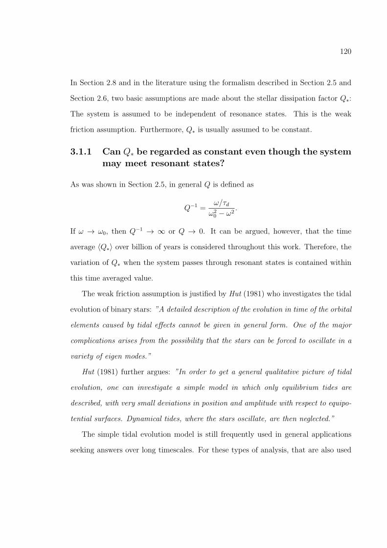
120
In Section 2.8 and in the literature using the formalism described in Section 2.5 and
Section 2.6, two basic assumptions are made about the stellar dissipation factor Q∗:
The system is assumed to be independent of resonance states. This is the weak
friction assumption. Furthermore, Q∗ is usually assumed to be constant.
3.1.1 Can Q∗ be regarded as constant even though the systemmay meet resonant states?
As was shown in Section 2.5, in general Q is defined as
Q−1 =ω/τd
ω20 − ω2
.
If ω → ω0, then Q−1 → ∞ or Q → 0. It can be argued, however, that the time
average ⟨Q∗⟩ over billion of years is considered throughout this work. Therefore, the
variation of Q∗ when the system passes through resonant states is contained within
this time averaged value.
The weak friction assumption is justified by Hut (1981) who investigates the tidal
evolution of binary stars: ”A detailed description of the evolution in time of the orbital
elements caused by tidal effects cannot be given in general form. One of the major
complications arises from the possibility that the stars can be forced to oscillate in a
variety of eigen modes.”
Hut (1981) further argues: ”In order to get a general qualitative picture of tidal
evolution, one can investigate a simple model in which only equilibrium tides are
described, with very small deviations in position and amplitude with respect to equipo-
tential surfaces. Dynamical tides, where the stars oscillate, are then neglected.”
The simple tidal evolution model is still frequently used in general applications
seeking answers over long timescales. For these types of analysis, that are also used

121
Figure 3.1: Left panel: Planetary revolution period versus semi major axis of a close-in extrasolar Jupiter analogue around a Sun-like star.Right panel: Planetary revolution rate versus semi major axis of a close-in extrasolarJupiter analogue around a Sun-like star.
in this work, simple models are parsimonious in providing sufficiently accurate pre-
dictions without the requirement to specify a high number of parameters.
Even if the model is found to be incorrect in some special cases, this failure in
itself would also be a valuable result. In such a case, the tidal evolution of the system
is strongly affected by dynamical tides (Zahn, 1977).
3.1.2 Can Q∗ be regarded as constant although it is definedas frequency dependent?
As a repetition, the definition of Q∗ for the weak friction assumption is given (Equa-
tion 2.5.7):
Q =|ω2
0 − ω2|ω/τd
(3.1.1)
where ω = 2(Ω∗ − n) is the tidal frequency and τd is the damping time scale.
With the equation given above, the assumption that Q∗ = const can be justified
for close-in extrasolar planets with semi major axes smaller than 0.05 AU by the
following arguments:

122
• For a < 0.05 AU, the planetary revolution rate n changes by one to two orders
of magnitude at most when the planet migrates toward the star (Figure 3.1).
• In many cases, the main sequence star in an extrasolar system rotates much
slower (typically with a rotation period between 10-100 days, see Section 2.10,
Figure 2.17) than the close-in planet revolves around the star (typically with a
revolution period of a few days, Figure 3.1). Therefore Ω∗ − n ≈ −n. In this
case, a < 0 (according to equation 2.6.17): The planet will migrate toward the
star.
• When comparing different possible values for the stellar dissipation factor Q∗
(Section 2.8), the possible values Q∗ given by different energy dissipation models
differ by several orders of magnitude. In the presence of such large uncertainties
in the mechanism of energy dissipation within the star, a possible variation of
Q∗, due to the underlying frequency dependency that is one to two orders of
magnitudes, can safely be neglected.
3.1.3 What happens with Q∗ when the system approachesdouble synchronicity?
For some exoplanetary systems discussed in this work, Ω∗ is similar to n. Later, in
Section 3.2, it will be shown that, in addition, the planetary rotation is probably
synchronized with the planet’s revolution, as well. Therefore, such systems may be
in a double synchronous state.
When the planetary system approaches this state, it follows from equation 2.5.7
that in the weak friction assumption, Q−1∗ → 0 or Q∗ → ∞. This strange result can
be explained by considering the problem in the reference system centered on the star

123
and rotating with it. The tidal wave on the star forms because mass elements inside
the star rearrange to accommodate the tidal potential of the planet and the subse-
quent change of the internal gravity potential of the star due to the tidal deformation.
Because the tidal bulge follows the planet as it revolves around the star, from the
viewpoint of the star, the tidal wave ’plows’ through the star with the effective fre-
quency ω = 2(Ω∗−n). This process generates friction, and energy is dissipated within
the star. More precisely, this can be envisioned at first order as a drag process within
a plasma environment. The force acting on a propagating wave is typically either
proportional to the velocity of the tidal wave v in the rotating frame or proportional
to the square of said velocity v2.
When ω = 0 and the orbit is circular, the tidal wave is stationary, no energy
is dissipated within the star (∆E over one cycle in the quotient of the definition of
Q (eq. 2.5.6) is zero), and no tidal friction takes place. Indeed, when looking at
equations (2.6.17) and (2.6.18), the terms are zero if Ω∗ = n. If the requirements
described in Section 2.9 are met, the system should remain in this equilibrium state
unless external forces disrupt the equilibrium state.
In this work, some possible double synchronous systems are investigated for which
Ω∗ − n is already very small. In this context, the constant Q∗ assumption may be
used again but for a different frequency regime than the non-synchronous cases for
which the tidal frequency is |ω| = 2|Ω∗ − n| ≈ |2n| ≈ 10−4 − 10−3s−1. In the double
synchronous state |ω| = 2|Ω∗ − n| ≈ 0.
Other systems will be investigated evolving from a state with Ω∗ > n to Ω∗ ≪
n, crossing the Ω∗ = n region. For these, the Q∗ = const assumption is at least
questionable. It will be shown, however, that the constant Q∗ may still be used in

124
this cases with some caveats.
It may be useful in the future to compare tidal friction models using a constant
stellar dissipation function Q∗ with tidal friction models using a constant tidal lag
time τ∗.
3.1.4 Switching from the constant Q- to the constant τ-formalism.
The derivation of the model described by Hut (1981) (Section 2.7) is identical to the
one described by Murray and Dermott (1999) (Section 2.6) if e = 0. The model by
Hut (1981) is, however, more general as it also describes tidal friction for bodies on
orbits with large eccentricities.
Apart from this, there is another major point where the formalisms deviate. As the
system evolves over time, the model of Hut (1981) keeps the tidal lag time τ∗ constant,
whereas the model described byMurray and Dermott (1999) regards the tidal lag angle
as ϵ or Q∗ constant. Both quantities are connected via 2ϵ = Q−1 = 2|Ω∗ − n|τ∗. As
long as the tidal frequency remains more or less constant during the whole evolution,
both models are equivalent.
Although the constant Q assumption is used in this work, one may easily switch
to constant τ -model by using well-known examples as ’calibration points’.
Switch from Q∗ to τ∗
The tidal dissipation factor Q∗k2,∗
is constrained for the OGLE-TR-56-system to be
Q∗k2,∗
≥ 2× 10⁷ (Carone and Patzold, 2007) and with k2,∗ = 0.018 this corresponds to
Q∗ ≥ 4 × 10⁵. The following parameters describe the OGLE-TR-56-system: M∗ =
1.17MSun, MPl = 1.3MJup, a = 0.0225 AU, and the stellar rotation period is P∗ =
19 days.

125
Consequently,
Ω∗ − n =2π
P∗−√G(M∗ +MPl)
a3(3.1.2)
=(3.8× 10⁻⁶ − 6.38× 10⁻⁵
)s−1
= −6× 10⁻⁵s−1.
From this, τ∗ can be calculated by:
τ∗ =1
2|Ω∗ − n|Q∗≈ 8333
Q∗s. (3.1.3)
Consequently, the lower limit of Q∗ = 4 × 10⁵ corresponds to a tidal lag time
τ∗ ≈ 2× 10⁻² s. In the following, the equation above will be used to switch from Q∗
to τ∗1.
Switch from QP to τP for jovian planets
The following ’calibration point’ can be used for the switch from the constant τPl to
a constant QPl formalism for jovian planets: The Jupiter-Io-example. Lainey et al.
(2009) derive QP
k2,P= 105 for Jupiter and, with k2,P l = 0.5, the tidal dissipation factor
is QPl = 5 × 10⁴. The rotation period of Jupiter is 9.925 hours, and the revolution
period of Io is 42.5 hours.
Consequently,
ΩPl − n =(1.8× 10⁻⁴ − 4× 10⁻⁵
)s−1 = 1.4× 10⁻⁴s−1. (3.1.4)
The tidal lag time τPl is:
τPl =1
QPl2|ΩPl − n|≈ 3600
QPl
s. (3.1.5)
1As a sidenote, the OGLE-TR-56 example illustrates that Ω∗ − n ≈ −n is indeed justified.

126
τPl and τ∗ differ only by a constant factor of about 2 because |Ω∗−n| and |ΩPl−n|
only differ by that factor. It follows that Jupiter, which experiences tides raised by Io,
as well as a main sequence star, which experiences tides raised by a close-in planet,
represent tidally oscillation systems with driving frequencies comparable in order.
Therefore, the Q-value derived in both cases and the underlying energy dissipation
mechanisms can be compared.
3.2 Is the planetary rotation tidally locked?
Throughout this work it is assumed that the planetary rotation is synchronized with
its revolution rate and that the planets therefore rotate relatively slow with rotation
periods of a few days. In other words, close-in extrasolar planets with semi major
axes a smaller than 0.1 AU are considered to be in the so-called tidally locked state.
This assumption can be tested by evaluating τsynchr, the time it takes for the
planetary rotation to become synchronized with its revolution. τsynchr is calculated
as (Murray and Dermott, 1999) for circular orbits (e = 0):
τsynchr =|n− ΩPl|
32
M∗MPl
(RPl
a
)3 GM∗a3
· IPlQPl
k2,P, (3.2.1)
where n is the planetary revolution rate, ΩPl is the primordial rotation rate of the
planet, IPl is the normalized moment of inertia of the planet, QPl is the planetary
dissipation constant and k2,P is the Love number of second order. Most of the stel-
lar and planetary parameters are determined by the combination of the transit and
radial velocity observations. Some planetary characteristics are unknown or poorly
constrained but can be estimated within reasonable ranges, as will be shown in the
following.
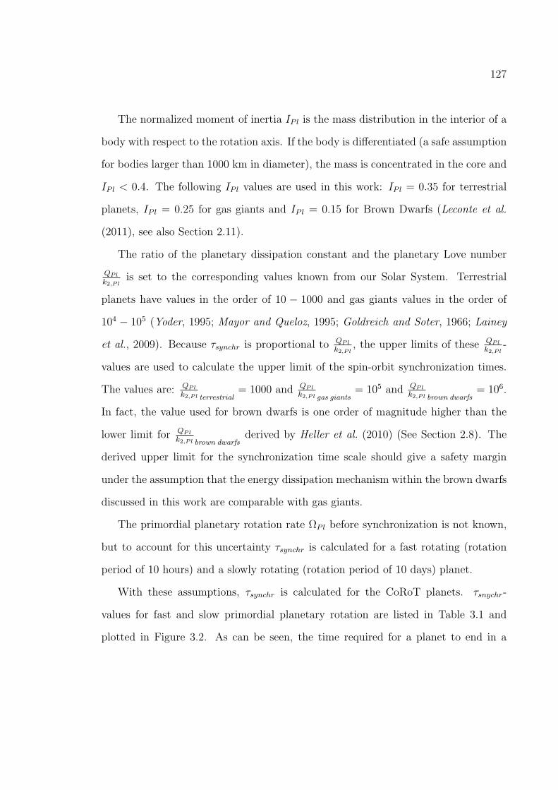
127
The normalized moment of inertia IPl is the mass distribution in the interior of a
body with respect to the rotation axis. If the body is differentiated (a safe assumption
for bodies larger than 1000 km in diameter), the mass is concentrated in the core and
IPl < 0.4. The following IPl values are used in this work: IPl = 0.35 for terrestrial
planets, IPl = 0.25 for gas giants and IPl = 0.15 for Brown Dwarfs (Leconte et al.
(2011), see also Section 2.11).
The ratio of the planetary dissipation constant and the planetary Love number
QPl
k2,P lis set to the corresponding values known from our Solar System. Terrestrial
planets have values in the order of 10 − 1000 and gas giants values in the order of
104 − 105 (Yoder, 1995; Mayor and Queloz, 1995; Goldreich and Soter, 1966; Lainey
et al., 2009). Because τsynchr is proportional to QPl
k2,P l, the upper limits of these QPl
k2,P l-
values are used to calculate the upper limit of the spin-orbit synchronization times.
The values are: QPl
k2,P l terrestrial= 1000 and QPl
k2,P l gas giants= 105 and QPl
k2,P l brown dwarfs= 106.
In fact, the value used for brown dwarfs is one order of magnitude higher than the
lower limit for QPl
k2,P l brown dwarfsderived by Heller et al. (2010) (See Section 2.8). The
derived upper limit for the synchronization time scale should give a safety margin
under the assumption that the energy dissipation mechanism within the brown dwarfs
discussed in this work are comparable with gas giants.
The primordial planetary rotation rate ΩPl before synchronization is not known,
but to account for this uncertainty τsynchr is calculated for a fast rotating (rotation
period of 10 hours) and a slowly rotating (rotation period of 10 days) planet.
With these assumptions, τsynchr is calculated for the CoRoT planets. τsnychr-
values for fast and slow primordial planetary rotation are listed in Table 3.1 and
plotted in Figure 3.2. As can be seen, the time required for a planet to end in a

128
tidally locked state is less than the systems age except for two cases: (a) CoRoT-9b,
the CoRoT-planet with the greatest semi major axis a = 0.407 AU and therefore the
CoRoT-planet that experiences the weakest stellar tidal forces, and (b) CoRoT-20b,
the youngest CoRoT-planet of an age of about 0.1 billion years that may not yet be
tidally locked.
Still this example shows that, unless the system is very young, planets with semi
major axes smaller than 0.1 AU can safely be assumed to be tidally locked. This
assumption is further supported by at least two observational evidences:
System τsynchr,slow rotator τsynchr,fast rotator IPlQPl
k2,P l
[106 years] [106 years]CoRoT-1 4× 10⁻⁴ 0.0013 0.2 105
CoRoT-2 0.02 0.0078 0.2 105
CoRoT-3 3 49 0.15 106
CoRoT-4 0.012 3 0.2 105
CoRoT-5 0.003 0.043 0.2 105
CoRoT-6 0.06 11.8 0.2 105
CoRoT-7 3× 10⁻⁵ 3.5× 10⁻⁵ 0.35 1000CoRoT-8 0.05 1.7 0.2 105
CoRoT-9 2.3× 10³ 6.3× 10⁴ 0.2 105
CoRoT-10 1 95 0.2 105
CoRoT-11 0.007 0.058 0.2 105
CoRoT-12 0.0022 0.018 0.2 105
CoRoT-13 0.032 0.47 0.2 105
CoRoT-14 0.008 0.024 0.2 105
CoRoT-15 2.9 26 0.15 106
CoRoT-16 0.01 0.27 0.2 105
CoRoT-17 0.029 0.34 0.2 105
CoRoT-18 0.0037 0.016 0.2 105
CoRoT-19 0.006 0.082 0.2 105
CoRoT-20 0.17 53 0.2 105
CoRoT-21 0.0075 0.058 0.2 105
Table 3.1: Synchronization time scale τsynchr for the CoRoT-planets. A slow rotatoris a planet with an initial rotation period PPl = 10 days, a fast rotator is a planetwith an initial rotation period of PPl = 10 hours.

129
Figure 3.2: Synchronization time scales τsynchr and the age of the CoRoT planetsversus their semi major axes. The black solid lines represent τsynchr calculated for aslow (10 days) and a fast (10 hours) primordial planetary rotation. The grey linesrepresent the system ages within the limit of uncertainties. The age of CoRoT-9b, aplanet orbiting its star beyond 0.4 AU, is represented by a dotted grey line. In thiscase, the system age and the possible synchronization time scale overlap each other.
The planetary emissions of υ Andromeda b (Harrington et al., 2006) and of
HD 189733 (Knutson et al., 2007) in the infrared show day/night variations con-
sistent with tidally locked planets. Figure (3.3) shows the substellar hot spot on the
planet. The day side is constantly heated by the star, the heating being strongest
at the substellar point. In contrast, the night side, which always points away from
the star, attains less heat via wind transfer from the day side. If the tidal locking
assumption would not be valid, the planet would show a more uniform heat emission
due to stellar irradiation over the whole surface.
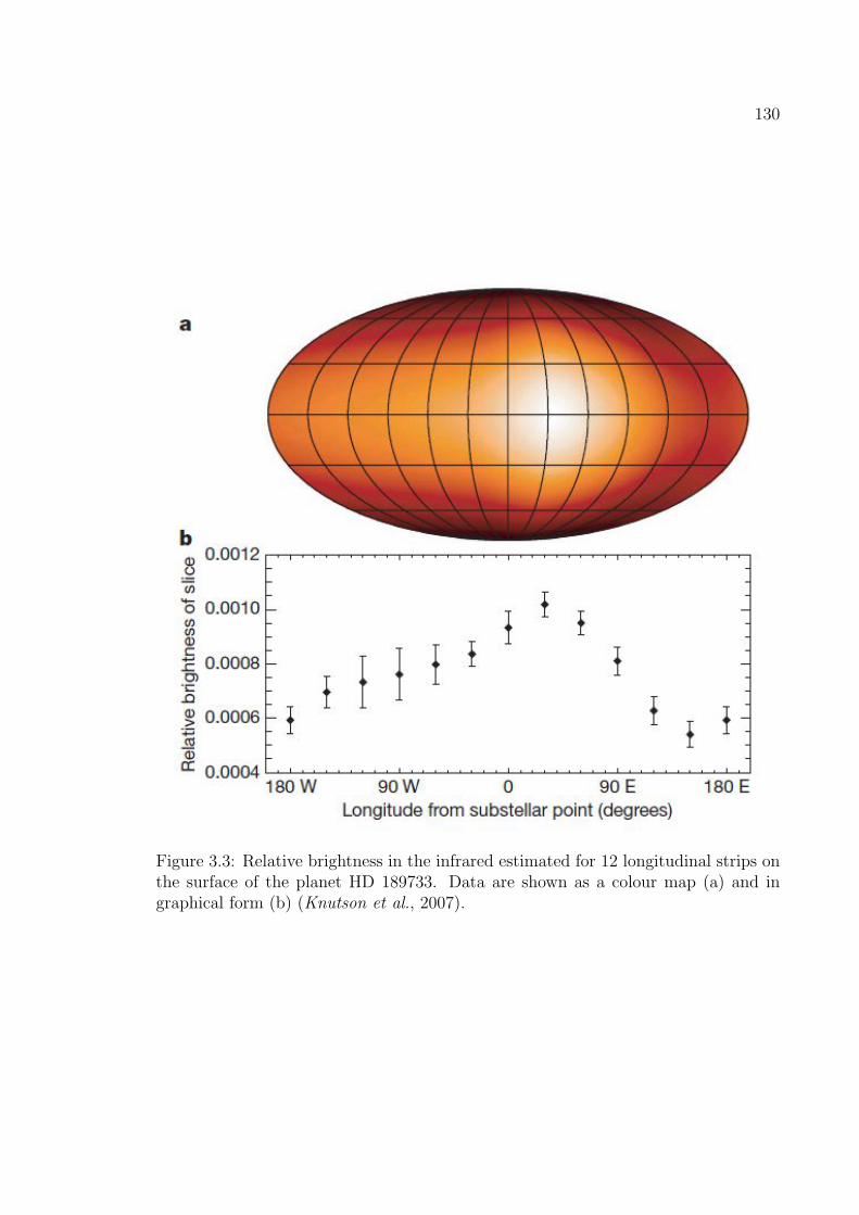
130
Figure 3.3: Relative brightness in the infrared estimated for 12 longitudinal strips onthe surface of the planet HD 189733. Data are shown as a colour map (a) and ingraphical form (b) (Knutson et al., 2007).

131
3.3 Energy and angular momentum in close-in ex-
trasolar planetary systems
It is useful to calculate the energies and angular momenta within a typical extraso-
lar system because these quantities ultimately determine the tidal evolution of the
system.
For this purpose, the following hypothetical test case is evaluated: An extrasolar
Jupiter analogue of mass MPl = 1MJup and radius RPl = 1RJup around a solar-like
star of mass and radiusM∗ = 1MSun, R∗ = 1RSun orbiting the star in a circular orbit
at semi major axis a = 0.02 AU is assumed.
The orbital energy is:
Eorbit = GMPlM∗
2a(3.3.1)
= 4.2× 1037J.
The stellar rotational energy is:
Erot,∗ =1
2I∗M∗R
2∗Ω
2∗ (3.3.2)
= 2.83× 1035J,
where Ω∗ is set to the rotation rate of the sun: Ω∗ = ΩSun = 2.9×10⁻⁶s−1 (Bouvier
et al., 1997) and the normalized moment of inertia is I∗ = 0.074 (see Section 2.11).
The planet’s rotational energy is:
Erot,P l =1
2IPlMPlR
2PlΩ
2Pl (3.3.3)
= 4.45× 1033J,
where the planet’s rotation rate is set to its revolution rate because spin-orbit synchro-
nization is expected: ΩPl = n =√G(M∗ +MPl)/a3 = 7× 10⁻⁵s−1. The normalized
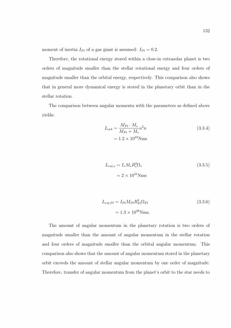
132
moment of inertia IPl of a gas giant is assumed: IPl = 0.2.
Therefore, the rotational energy stored within a close-in extrasolar planet is two
orders of magnitude smaller than the stellar rotational energy and four orders of
magnitude smaller than the orbital energy, respectively. This comparison also shows
that in general more dynamical energy is stored in the planetary orbit than in the
stellar rotation.
The comparison between angular momenta with the parameters as defined above
yields:
Lorb =MPl ·M∗
MPl +M∗a2n (3.3.4)
= 1.2× 1042Nms
Lrot,∗ = I∗M∗R2∗Ω∗ (3.3.5)
= 2× 1041Nms
Lrot,P l = IPlMPlR2PlΩPl (3.3.6)
= 1.3× 1038Nms.
The amount of angular momentum in the planetary rotation is two orders of
magnitude smaller than the amount of angular momentum in the stellar rotation
and four orders of magnitude smaller than the orbital angular momentum. This
comparison also shows that the amount of angular momentum stored in the planetary
orbit exceeds the amount of stellar angular momentum by one order of magnitude.
Therefore, transfer of angular momentum from the planet’s orbit to the star needs to

133
be treated with care. It cannot be readily neglected because it affects the evolution of
stellar rotation. Furthermore, it is justified to neglect the planet’s rotation about its
spin-axis when calculating the long-term dynamical evolution of the planetary system
due to tidal interactions between the planet and the star.
3.3.1 Possible pitfalls in the calculation of the Roche zone
The approximations (eq. 2.12.10) and (eq. 2.12.8) used in Section 2.12 to calculate
the Roche zone are used if the planet’s density is unknown. The equations, however,
are valid only if(
ρ∗ρPl
)1/3≈ 1 which is true for Solar System gas giants and the Sun.
The calculation of the Roche limits with the true density derived from transiting
exoplanets, however, may shed light onto the limitations of these approximations.
The Roche limits aRoche,spher . and aRoche,hydro. are computed for some CoRoT plan-
ets for which the stellar and planet’s density are known and listed in Table 3.2. Their
parameters are listed in Section 1.4. As can be seen, for some systems the assump-
tion 3√ρPl ≈ 3
√ρ∗ holds, but for many other systems it doesn’t. Figure 3.4 shows the
density of all transiting exoplanets in units of Jupiter density. For example, several
exoplanets have been found with average densities much smaller than the density of
Jupiter 2. Brown dwarfs (CoRoT-3b and CoRoT-15, for example), on the other hand,
don’t satisfy the 3√ρPl ≈ 3
√ρ∗-assumption because they are much denser than Jupiter
planets. These objects lie in the transition region between the mass regimes of gas
giants and the smallest stars (see Section 1.1). An object in the ’brown Dwarf desert’
is approximately the size of Jupiter although it may contain up to eighty Jupiter
masses.
2The mechanism responsible for the inflation of some short-period extrasolar gas giants is stilldisputed.

134
Figure 3.4: Density of transiting exoplanets versus their mass.
If the planet is inflated, the extent of the Roche zone is underestimated. If the
companion is a brown dwarf or a terrestrial planet like CoRoT-7b, the extent of the
Roche zone is overestimated. This needs to be considered when using (eq. 2.12.10)
and (eq. 2.12.8).
As a side remark, it is interesting to note that the ’true’ Roche zone of Brown
Dwarfs lies within the star; see the derived Roche limits of CoRoT-3b and CoRoT-
15b (Table 3.2). This would mean that brown dwarfs can approach their stars and
be engulfed by them without being tidally disrupted during their approach.

135
System aRoche,spher. aRoche,hydro ρ∗ ρPl (ρ∗/ρPl)1/3
[R∗] [R∗] [ρSun] [ρJup]CoRoT-1 1.86 3.19 0.70 0.32 1.27CoRoT-2 1.54 2.63 1.32 1.08 1.05CoRoT-3 0.37 0.63 0.36 21.65 0.25CoRoT-4 1.70 2.91 0.73 0.44 1.16CoRoT-5 2.15 3.67 0.59 0.18 1.46CoRoT-6 1.15 1.96 0.98 1.92 0.78CoRoT-7 0.90 1.54 1.65 6.73 0.61CoRoT-8 1.68 2.86 1.93 1.22 1.14CoRoT-9 1.68 2.88 1.19 0.75 1.15CoRoT-10 1.20 2.05 1.81 3.10 0.82CoRoT-11 1.22 2.08 0.49 0.82 0.83CoRoT-12 1.94 3.31 0.77 0.32 1.32CoRoT-13 1.18 2.01 1.06 1.94 0.80CoRoT-14 0.82 1.41 1.13 6.04 0.56CoRoT-15 0.30 0.51 0.42 46.40 0.21
Table 3.2: Comparison of Roche limit approximations

Chapter 4
Close-in extrasolar planets asplayground for tidal friction models
This work focuses on tidal friction due to tides raised by the planet on the star (stellar
tidal friction) and on the consequences for the exoplanet’s semi major axis and the
stellar rotation. As derived from Sections (2.6) and (2.7), massive exoplanets with
very short semi major axes are the most interesting in this context. It will be shown
that the planetary systems discovered by CoRoT provide an ideal playground for
investigating tidal evolution and to derive constraints on Q∗k2,∗
.
4.1 The tidal stability maps for planets around
main sequence stars
In most cases, an extrasolar planet with semi major axis less than 0.1 AU revolves
faster about the star than the star rotates (Ω∗ < n). Therefore, tidal friction as a
result of the delay of the tidal bulge on the star leads to a decrease in the planet’s
semi major axis and consequently to the spin-up of the star. The planet may even
reach the Roche zone and may be destroyed there (Section 2.12). It is worthwhile
investigating which Q∗k2,∗
is required for a planet to reach the Roche limit within the
136

137
planetary system’s lifetime and how many planets may be destroyed due to tidal
friction.
The time τRoche it takes for a planet on a circular orbit to reach the Roche zone
due to tidal friction can be calculated by (Patzold and Rauer, 2002):
τRoche =
113
[a13/2Present − a
13/2Roche
]3k2,∗MPl
2Q∗M∗R5
∗√GM∗
, (4.1.1)
where aPresent is the current semi major axis of the planet, aRoche is the Roche limit,
MPl is the planet’s mass, M∗ and R∗ are the stellar mass and radius, respectively, G
is the gravitational constant, Q∗ is the stellar tidal dissipation factor and k2,∗ is the
stellar Love number.
As was explained in Section 2.12, several estimates exist for the Roche limit. Here,
aRoche,hydro = 2.46R∗
(ρ∗ρPl
)1/3, which defines the outer boundary of the ’Roche zone’,
is used for the calculation of τRoche.
Of all the parameters needed to calculate τRoche, the ratio of the stellar tidal
dissipation factor over Love number Q∗k2,∗
is the least constrained. Indeed, estimates
of the stellar dissipation factor cover several orders of magnitude. In the following,
a Q∗k2,∗
between 105 and 109 is assumed to cover the whole range of estimates of the
amount of tidal energy dissipated within a main sequence star (See Section 2.8.2).
τRoche is calculated here under the constant Q∗ assumption. As outlined in Sec-
tion 3.1.2, the validity of this assumption requires the following: The star rotates
much slower than the planet revolves around it (Ω∗ ≪ n) to satisfy the approxi-
mation (Ω∗ − n) ≈ −n, where 2(Ω∗ − n) is the tidal frequency. Furthermore, the
revolution rate n should remain approximately constant throughout the calculation.

138
As was outlined in Section 3.1.2, n varies by one and a half order of magnitude be-
tween 0.02 and 0.15 AU which is acceptable given the large uncertainties of Q∗. The
time scale τRoche will now be investigated systematically for different ’model’ planets
placed in close proximity to the star.
At the center of these model planetary systems, a main sequence star of spectral
type K, G, and F is placed. For each spectral type, there exists a CoRoT exoplanet
host star (Table 1.2). One of these was selected as a representative of spectral type
K and F (Table 4.1). For spectral type G, the Sun was selected as a representative to
show that the investigation of tidal interactions in extrasolar planetary systems helps
to place our own Solar System in a greater context and to potentially learn something
about solar properties. If Q∗k2,∗
is constrained for a solar-like star, this result is also
applicable to energy dissipation processes within our Sun.
Spectraltype
name Teff mass radius reference
[K] [MSun] [RSun]K1V CoRoT-8 5080 0.88 0.77 Borde et al. (2010)G2V Sun 5780 1 1 Unsoeld and Baschek (2001)F7V CoRoT-15 6350 1.32 1.46 Bouchy et al. (2011)
Table 4.1: The parameters of the central stars used for the calculation of the tidalstability maps. Real stars were selected as representatives of K-, G- and F-spectraltype stars, respectively.
The following exoplanets are investigated exemplarily for each star: A high-
mass Brown Dwarf (HBD) like CoRoT-15b, a low-mass Brown Dwarf like CoRoT-3b
(LBD), a hot Jupiter (HJ) like CoRoT-1b, an extrasolar hot Neptune analogue planet
(HN), an extrasolar Super Earth like CoRoT-7b (SE), an extrasolar Earth analogue
planet (EE) and an extrasolar Mercury analogue planet (EM). See Table 4.2 for their
parameters.

139
Exoplanet type name mass radius reference[MJup] [RJup]
High massbrown dwarf
CoRoT-15b 63 1.12 Bouchy et al. (2011)
low mass browndwarf
CoRoT-3b 21.66 1.01 Deleuil et al. (2008)
hot Jupiter CoRoT-1b 1.03 1.49 Barge et al. (2008)hot Neptune Neptune 0.054 0.36 Unsoeld and Baschek
(2001)Super Earth CoRoT-7b 0.023 0.15 Hatzes et al. (2011),
Bruntt et al. (2010)Exo-Earth Earth 0.0032 0.092 Unsoeld and Baschek
(2001)Exo-Mercury Mercury 1.74× 10⁻⁴ 0.035 Unsoeld and Baschek
(2001)
Table 4.2: The parameters of the exoplanets placed around each star (Table 4.1) forthe calculation of the tidal stability map. A real planet was selected as a representativefor each exoplanet category.
Now τRoche is calculated for planets with semi major axis greater than aRoche,hydro
but within 0.15 AU and for Q∗k2,∗
= 105−109. τRoche is compared with the total lifetime
of the star, the time for which the star remains on the main sequence. It is reasonable
to investigate if a planet will survive during that time.
For main sequence stars, the stellar lifetime can be calculated approximately by
(Prialnik, 2000):
T0 = 1010(
M∗
MSun
)−2.8
years. (4.1.2)
With these assumptions, ’tidal stability maps’ can be calculated (Figures 4.1, 4.2,
and 4.3). They show unstable semi major axes for combinations of specific planets
and stars in dependence of Q∗k2,∗
. Instability herein means that the planet may reach
the Roche zone within the remaining lifetime. Furthermore, athreshold is given for each
Q∗k2,∗
= 105 − 109 that is the semi major axis where τRoche equals the total lifetime of
140
the central star.
Planets within athreshold are the most interesting ’test cases’ for different stellar
tidal dissipation models as these systems should be affected by tidal friction on as-
tronomical time scales. As can be seen (Figures 4.1, 4.2, and 4.3), the more massive
the planet and also the more massive the host star, the further outwards extends
the region of orbital instability. In addition, when comparing the parameters of the
CoRoT planetary systems (Tables 1.3 and 1.2) with the tidal stability maps, it will
become apparent that several CoRoT planets lie in unstable regions.

141
Figure 4.1: Tidal stability maps for different exoplanets around a K-star. From top tobottom, from left to right: A high mass brown dwarf, a low mass brown dwarf, a hotJupiter, a Neptune, a Super-Earth, an Earth and a Mercury planet. The grey colorgives the time scale τRoche in log(109 years). The total lifetime of the star is indicatedas a white dashed line. The black lines are the isochrones of τRoche. The horizontaland vertical dashed white lines indicate the stability limit athreshold for every Q∗
k2,∗.

142
Figure 4.2: Tidal stability maps for different exoplanets around a G-star. See alsoFigure 4.1.

143
Figure 4.3: Tidal stability maps for different exoplanets around an F-star. See alsoFigure 4.1.

144
4.1.1 CoRoT systems most strongly affected by tidal friction
It became apparent in the previous section that the majority of the orbits of the
majority of the CoRoT planets would be unstable under tidal friction for Q∗k2,∗
= 105.
There are four clear cases that are stable for all assumed values of Q∗k2,∗
= 105 − 109
because their semi major axes are greater than the respective athreshold: CoRoT-4b,-
6b,-8b, and -9b. CoRoT-16b lies barely below athreshold for Q∗k2,∗
= 105. CoRoT-20b
and CoRoT-10b appear at first glance to be stable. Their orbits, however, are in
contrast to most other CoRoT planets very eccentric. Subsequent chapters will show
that these planets are sufficiently long in the unstable regions to be affected by tidal
friction.
Apart from the tidal stability maps, there are two other parameters that can be
used to identify systems strongly affected by tidal friction: the Doodson constant Do
and the tidal property factor PF .
The Doodson constant
The Doodson constant (see Doodson (1921) and Patzold et al. (2004)) is defined as:
Do =3
4
GMPl
a3R2
∗. (4.1.3)
This is the amplitude of the tidal potential (equation 2.3.8) and is a direct measure
of the strength of the tidal force acting on the star 1. Figure 4.4 shows the Doodson
constant for tides raised by the CoRoT-planets on their stars. In comparison some
Doodson constants are given for the Solar System.
Compared to tidal forces in the Solar System (Earth-Moon, Sun-any planet), the
tidal forces between the CoRoT stars and planets are orders of magnitudes larger.
1The factor 3/4 arises to ensure that the amplitude of the angle dependent part of the tidalpotential, that is the Legendre polynomial of second order P2(cos θ), is scaled to unity.

145
Figure 4.4: Doodson constants for tides raised on the star by CoRoT-1 to CoRoT-21band several Solar System bodies. M marks the Doodson constant for tides raised bythe Earth on the Moon, E denotes the Doodson constant for lunar tides raised onEarth, J denotes tides raised by Jupiter on the Sun and Me denotes the Doodsonconstant for tides raised by Mercury on the Sun.
CoRoT-planets are much closer to their stars than the planets in the Solar System.
Mercury, the innermost planet in the Solar System, orbits at a = 0.387 AU. In
addition, many CoRoT-planets are massive objects like gas giants and Brown Dwarfs.
In the Solar System, the gas giants orbit far away from the Sun. Jupiter, the innermost
gas giant, orbits at a = 5.2 AU. Within the CoRoT planetary systems, the following
planets stand out due to their large Doodson numbers: CoRoT-1b,-2b,-3b,-14b,-15b,-
18b, and -21b. In contrast to that, CoRoT-4b,-8b,-10b, and especially CoRoT-9b are
the CoRoT planets with the smallest Doodson constant. CoRoT-9b is the transiting
planet with the largest semi major axes found to date, therefore, the small Doodson
number comes as no surprise. CoRoT-4b was already identified by the stability maps
as a planetary system where planetary tides raised on the star have little consequences.
The Doodson constant of CoRoT-10b, on the other hand, may be misleading due to

146
CoRoT-10b’s large orbital eccentricity and because the Doodson constant is only valid
for circular orbits.
The tidal property factor
The tidal property factor PF determines the secular orbital change (equation 2.6.19)
and is described in Patzold and Rauer (2002):
PF =MPl√M∗
R5∗. (4.1.4)
Figure 4.5: The tidal property factor for tides raised by the planets CoRoT-1b toCoRoT-21b on their stars.
Figure 4.5 shows the property factor for tides raised by the CoRoT planets and
their stars. Four planets stand out: The brown dwarfs CoRoT-3b and CoRoT-15b
have by far the largest property factor and reflect the fact that the mass ratio between
the star and these companions is unusually high compared to other extrasolar planet
systems. Consequently, it comes as no surprise that the least massive CoRoT planet,
the Super Earth CoRoT-7b, has the lowest property factor. CoRoT-8b on the other

147
hand has such a small property factor because it orbits the smallest CoRoT exoplanet
host star. CoRoT-8 is a K star with a radius of only 0.77RSun.
In short, planetary companions, that stand out due to their large tidal property
factor or Doodson constant or that lie in the unstable region of the tidal stability
map, are particularly worthwhile candidates for tidal interaction investigations. This
would be here: The brown dwarfs CoRoT-3b and CoRoT-15b, the jovian exoplanets
CoRoT-1b,-2b,-3b, -5b,-11b,-13b,-14b,-18b,-19b, and -21b with semi major axis be-
tween 0.0254 AU and 0.057 AU. The tidal evolution of the Super Earth CoRoT-7b
at a = 0.0172 AU is worthwhile investigating, as well. The tidal stability maps show
that the planet lies in an unstable region around its star making it a worthwhile
candidate for tidal interaction investigations even though it has the smallest prop-
erty factor and a comparatively small Doodson constant. This example shows that,
strictly speaking, a comparison of Doodson constants and property factors is better
reserved for planets of the same class. Otherwise one may incorrectly judge a Super
Earth to be an unsuited object for tidal interaction investigations when it is directly
compared with much more massive Brown Dwarfs.
CoRoT-4b,-6b,-8b,and -9b have large semi major axes a = 0.063 − 0.407 AU,
which lie in the stable regions of the tidal stability and have small tidal property
factors and Doodson constants. For these systems, tidal friction is expected to play
a minor role in their dynamical evolution.
When comparing the stellar rotation periods with the revolution periods (Ta-
ble 1.4), many CoRoT systems are identified for which the stellar rotation is slower
than the planetary revolution which may lead to the planet’s migration towards the
star, as expected. For other systems, however, this assumption does not hold: In

148
the CoRoT-6, CoRoT-11 and CoRoT-9 system, the stellar rotation is faster than the
planet’s revolution, consequently, the planet may migrate away from the star. Fur-
thermore, the stellar rotation and planetary revolution appears to be very similar
in the CoRoT-3, CoRoT-4, CoRoT-15 system, and maybe the CoRoT-20 system,
which marks them as potential double synchronous states. Finally, four systems are
identified with substantial orbital eccentricity e = 0.3− 0.562: CoRoT-9, CoRoT-10,
CoRoT-16, CoRoT-20. These are worthwhile investigating for this fact alone.
In summary, the CoRoT planets not only present a number of systems potentially
unstable under tidal friction. In addition, many more scenarios with very different
parameter constellations are encountered, worthwhile investigating in terms of tidal
interactions. Consequently, the CoRoT-planetary systems can be divided into five
categories which will be investigated separately in the course of this work:
• Planets on circular orbits around slowly rotating low-mass stars: CoRoT-1b,
CoRoT-2b, CoRoT-7b, CoRoT-8b, CoRoT-12b, CoRoT-13b, CoRoT-17b, and
CoRoT-18b.
• Planets on circular orbits around slowly rotating F-stars and one subgiant:
CoRoT-5, CoRoT-14b, CoRoT-19b, and CoRoT-21b (around a subgiant)
• Planets on eccentric orbits: CoRoT-9b, CoRoT-10b, CoRoT-16b, and CoRoT-
20b.
• Planets around fast-rotating stars: CoRoT-6b and CoRoT-11b
• Possible double synchronous systems: CoRoT-3, CoRoT-4, CoRoT-15, and
CoRoT-20.

Chapter 5
Constraining Q∗k2,∗
by requiring
orbital stability of close-in planetsaround slowly rotating stars
In this chapter, the tidal semi major axes evolution of planets around slowly rotating
stars is investigated. The constant-Q∗-assumption is justified at least for systems
with planets on circular orbits because Ω∗ − n < 0 during the whole evolution time
and because Ω∗−n does not vary by more than one and a half orders of magnitude at
most during the whole evolution time. This is verified in Chapter 6 that investigates
the stellar rotation evolution and in the Appendix (Figures C.1, C.2, C.3, and C.4).
The planets discussed here may migrate towards their star and even enter the Roche
zone within the lifetime of the star. It will be investigated for which Q∗k2,∗
the system
may be regarded as stable.
149

150
5.1 Tidal evolution of the semi major axis of CoRoT-
Planets on circular orbits
Because the star rotates more slowly than the planet revolves around it (Ω∗ < n), the
evolution of a planet’s semi major axis on a circular orbit is modeled by:
a = −3k2,∗MPl
Q∗M∗
(R∗
a
)5
na (5.1.1)
according to Section 2.6, Eq. (2.6.17). In Chapter E, the integration method used in
this work is described and in Chapter F a model sensitivity analysis is performed for
several selected CoRoT-systems.
The start time of the semi major axis evolution was set to 60 million years because
at this age the inner structure of the CoRoT stars has settled (see Section 2.10,
Figure 2.15). Even in cases where the minimum age cannot be constrained further
by observations (CoRoT-1), this gives the lower limit for the age. The end time of
the evolution was set to 1.5 × 10¹⁰ years to accommodate even the system with the
largest lifetime and to keep the evolution of all systems comparable. The results of
the semi major axis evolution are discussed in terms of the remaining lifetime, the
total lifetime of each system minus the estimated age.
The semi major axis evolution is calculated for Q∗k2,∗
= 105− 109 to account for the
uncertainty of the stellar tidal dissipation factor. Furthermore, QPl
k2,P l= 105 is assumed
for the tidal evolution of Jupiter-like planets on circular orbits in agreement with
calculations in Section 3.2. These planets can be regarded as tidally locked (ΩPl = n)
and tidal friction due to tides raised on the planet by the star is neglected1.
1For the Super-Earth CoRoT-7, QPl = 10−100 is probably more realistic, in agreement with QPl
found for terrestrial bodies in our own Solar System. For the investigations in this work, this onlymeans that the planet’s rotation is more easily synchronized with the planet’s revolution. Therefore,

151
In the following, planets around low mass and higher mass stars are discussed
separately. The need for this additional sub-division will become clear when discussing
the stellar rotation evolution due to tidal friction in Chapter 6.
5.1.1 Tidal evolution of the semi major axis of CoRoT-Planetson circular orbits around low mass stars
CoRoT systems with a close-in planet on a circular orbit and a low mass star (M∗ <
1.1MSun) are: CoRoT-1, CoRoT-2, CoRoT-7, CoRoT-8, CoRoT-12, CoRoT-13, CoRoT-
17, and CoRoT-18. The eccentricities of the orbits of CoRoT-12b and CoRoT-18b
are sufficiently small (e = 0.07 ± 0.06 and e ≤ 0.08, respectively) that they can be
assumed to be zero, as well.
Figure 5.1 shows the evolution of the planets’ semi major axis for the next 1.5×10¹⁰
years into the future with the equation (5.1.1) given above. The vertical lines mark
how much time is left until the star evolves away from the main sequence, i.e., until
its hydrogen fuel is depleted enough so that the star changes its inner structure
dramatically in very short time, astronomically speaking (see for example Unsoeld
and Baschek (2001)). The estimated total lifetime is listed in Table 5.12. For CoRoT-
17, the estimated total lifetime is actually smaller than the age of the system. This is
not surprising because the relation by Prialnik (2000) (Eq 4.1.2) is a very simplified
estimate that can be ’off’ by one to two billion years. When taking into account,
however, the error bars for the age of main sequence stars (Table 5.1), it becomes
apparent that such a deviation is acceptable.
As can be seen from Figure 5.1, CoRoT-8 is the only planet within this subsample
it is a safe assumption that CoRoT-7b is tidally locked, as well.2The age of CoRoT-1 is unknown. Therefore, the system is assumed to be at the beginning of
its evolution.

152
Figure 5.1: The tidal evolution of the semi major axis of the planets CoRoT-1b,-2b, -7b, -8b, -12b, -13b, -17b and -18b for the next 1.5 × 10¹⁰ years and forQ∗k2,∗
= 105 − 109. The horizontal lines mark Roche limits (from top to bottom:
aRoche,hydro, aRoche,inter, aRoche,rigid) which span the Roche zone (Section 2.12). At thedistance a = 1R∗, another horizontal line marks the stellar surface. The verticalgrey lines show the remaining lifetime of the system. The solid vertical line is thetotal lifetime of the star computed by 4.1.2 minus the age of the system. The dot-ted vertical lines are the minimum and maximum remaining lifetime of the system(lifetime− age±∆age). For CoRoT-1, no age is known. A black vertical line marksthe total lifetime. CoRoT-17 has reached the end of its lifetime, this is indicated bya black vertical line at the start point of the evolution.

153
which does not change its semi major axis significantly for any investigated Q∗k2,∗
=
105 − 109 during the next 15 billion years. This was already inferred in the previous
Chapter 4.1.1 by the tidal stability map, the Doodson constant and the property
factor. Apparently, these three measures are useful in distinguishing between tidally
evolved and tidally stable systems.
CoRoT-1b, -2b, -7b, -13b, and -18b, on the other hand, may become unstable
within the remaining lifetime of the system. CoRoT-12b and CoRoT-17b, whose
stars may already be at the end of their lifetime, can still be considered as unstable
if Q∗k2,∗
= 105, in which case these planets may enter the Roche zone on timescales of
ten to hundred million years. This is a fate they share with CoRoT-1b, -2b, -7b and
-18b.
This is very short when compared to the remaining lifetime of several billion years.
It would be unlikely to observe such planets just as they plunge toward their host
star, but detections of close-in hot Jupiters are by no means rare events. Intuitively,
Q∗k2,∗
would be expected to be much higher than 105 to allow long-term survival for
such very short-period extrasolar planets. The same conclusion may be tentatively
drawn for Super-Earths like CoRoT-7b. The Kepler-10 system, for example, has very
similar properties to CoRoT-7 with one noteworthy exception (Batalha et al., 2011):
Kepler-10 (age: 12 billion years) is about ten billion years older than CoRoT-7 (age:
1-2 billion years). Kepler-10b looks like an older version of CoRoT-7b, which also
hints to a long-term stability of such systems.
The Q∗k2,∗
-limit of stability necessary for a given planet to survive under tidal friction
can be derived more accurately by setting the remaining lifetime τrem.lifetime = τRoche,

154
inserting it into equation 4.1.1 and by solving for Q∗k2,∗
:
Q∗
k2,∗ stable≥τrem.lifetime
3MPl
2M∗R5
∗√GM∗
113
[a13/2Present − a
13/2Roche
] , (5.1.2)
where τrem.lifetime is the estimated total lifetime minus the age of the system (Ta-
ble 5.1), for the Roche limit aRoche, the outermost limit of the Roche zone was se-
lected aRoche,hydro = 2.46R∗
(ρ∗ρPl
)1/3, and aPresent is the current semi major axis of
the planet.
The derived limits of stability are given in Table 5.1. It should be noted that for
CoRoT-12b, a confidence interval of the estimated stability is computed due to the
large uncertainty in the age of the system. The given values represent the stability
limit for the minimum, average and maximum remaining lifetime. The minimum
estimated remaining lifetime of CoRoT-12 is zero because the system may already be
at the end of its lifetime. Q∗k2,∗
= 107 − 108 emerges as a common limit of stability
from Table 5.1.
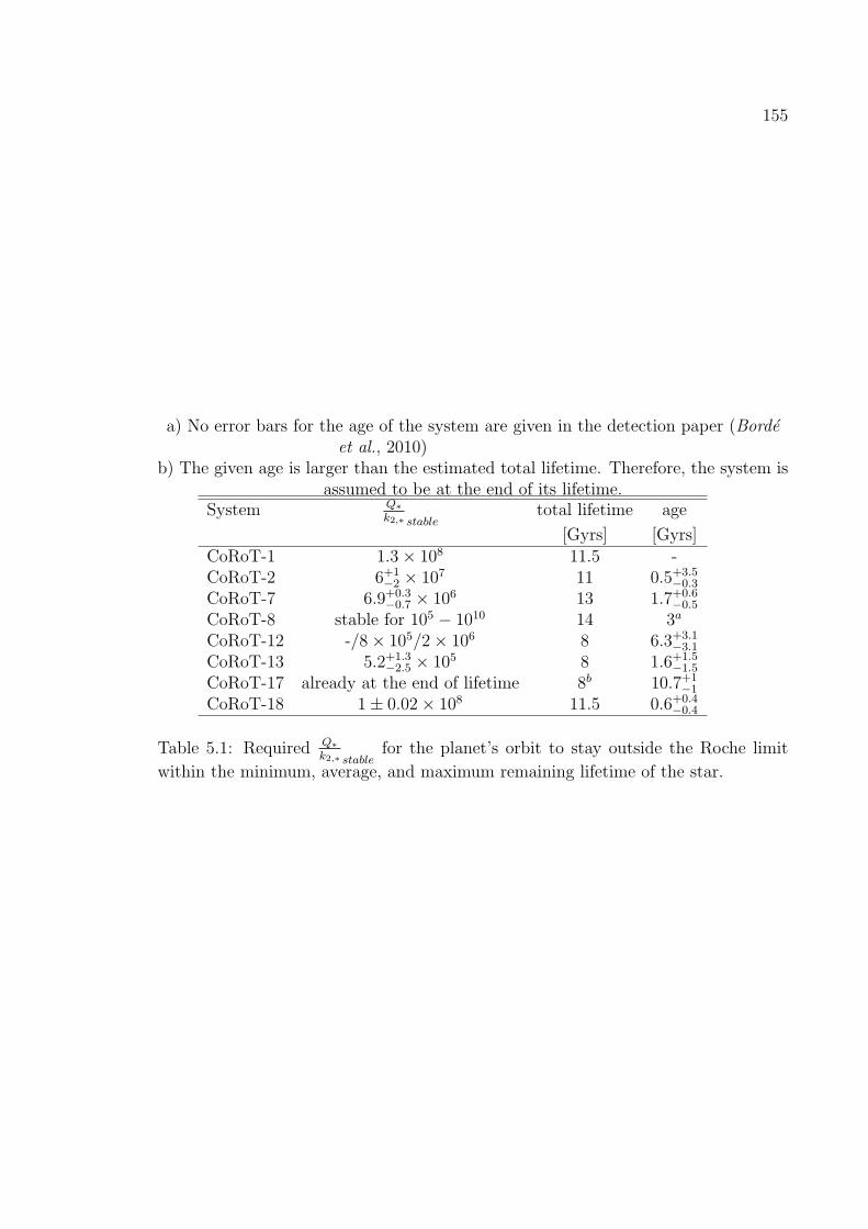
155
a) No error bars for the age of the system are given in the detection paper (Bordeet al., 2010)
b) The given age is larger than the estimated total lifetime. Therefore, the system isassumed to be at the end of its lifetime.
System Q∗k2,∗ stable
total lifetime age
[Gyrs] [Gyrs]CoRoT-1 1.3× 10⁸ 11.5 -CoRoT-2 6+1
−2 × 10⁷ 11 0.5+3.5−0.3
CoRoT-7 6.9+0.3−0.7 × 10⁶ 13 1.7+0.6
−0.5
CoRoT-8 stable for 105 − 1010 14 3a
CoRoT-12 -/8× 105/2× 106 8 6.3+3.1−3.1
CoRoT-13 5.2+1.3−2.5 × 10⁵ 8 1.6+1.5
−1.5
CoRoT-17 already at the end of lifetime 8b 10.7+1−1
CoRoT-18 1± 0.02× 10⁸ 11.5 0.6+0.4−0.4
Table 5.1: Required Q∗k2,∗ stable
for the planet’s orbit to stay outside the Roche limit
within the minimum, average, and maximum remaining lifetime of the star.

156
5.1.2 Tidal evolution of the semi major axis of planets oncircular orbits around F stars and subgiants
The orbit stability of the CoRoT-planets on circular orbits around F-stars is inves-
tigated: These are CoRoT-5b, CoRoT-14b, CoRoT-19b, and CoRoT-21b orbiting a
subgiant.
Figure 5.2: The tidal evolution of the semi major axis of the planets CoRoT-5b, 14b,19b, and -21b for the next 1.5 × 10¹⁰ years and for Q∗
k2,∗= 105 − 109. The horizontal
lines span the Roche zone. The horizontal line at a = 1R∗ marks the stellar surface.The vertical lines show the remaining lifetime of the system. See Figure 5.1 for amore detailed description.
Figure 5.2 shows the evolution of the planets’ semi major axes. All planets inves-
tigated in this subsection may reach the Roche zone within their remaining lifetime.

157
System Q∗k2,∗ stable
total lifetime age
[Gyrs] [Gyrs]CoRoT-5 2.7+1.2
−1.2 × 10⁵ 10 6.9+1.4−1.4
CoRoT-14 -/9× 107/1.9× 108 7.1 4+4−3.6
CoRoT-19 -/6.3× 105/1.4× 106 5.9 5+1−1
CoRoT-21 1+0.2−0.6 × 10⁷ 4.9 4.1+0.5
−0.1
Table 5.2: Required Q∗k2,∗ stable
(eq. 5.1.2) for the planet’s orbit to stay outside the Roche
limit within the remaining lifetime of the star.
The age of CoRoT-14 and -19 are not very well constrained and it cannot be excluded
that the systems are already at the end of their lifetimes. Strictly speaking, Q∗k2,∗
can-
not be constrained by requiring the planets CoRoT-14b and -19b to survive for the
next few billion years. Still, the CoRoT-14 system would already be destroyed within
the next few hundred million years if Q∗k2,∗
≤ 107. The same is true for CoRoT-21b.
If Q∗k2,∗
is indeed as small as 105, it should be unlikely to observe such systems on the
’brink of destruction’.
Equivalent to the approach in the previous section, Q∗k2,∗ stable
is calculated as a
lower limit that would allow the planet to survive the remaining lifetime under tidal
friction (Table 5.2).
Again, Q∗k2,∗
= 107 − 108 emerges as a common limit of stability; even though the
systems in this subset have much shorter lifetimes than the systems with low mass
stars, discussed previously (Table 5.1)

158
5.2 Tidal evolution of the semi major axis and ec-
centricity of planets on eccentric orbits
The following CoRoT-systems with non-negligible orbit eccentricity are identified:
CoRoT-9, CoRoT-10, CoRoT-16 and CoRoT-20. CoRoT-9b’s semi major axis, how-
ever, is so great that no substantial orbital evolution is expected. Furthermore,
CoRoT-9 rotates much faster than the planet revolves around it. Consequently, even
if tidal friction would be a factor in the system’s evolution, it would drive the planet
away from the star. That tidal friction plays no role in the orbital evolution of
CoRoT-9b is confirmed by the computation (Appendix, Figure B.2). In the follow-
ing, the semi major axis and eccentricity evolution of CoRoT-10b, CoRoT-16b and
CoRoT-20b are investigated in more detail.

159
The relevant set of equations are:
da
dt=− 3
k2,∗Q∗
MPl
M∗
(R∗
a
)5
na(1− e2)−15/2
[f1(e)n− (1− e2)3/2f2(e)Ω∗
]|n− Ω∗|
− 3k2,P l
QPl
M∗
MPl
(RPl
a
)5
na(1− e2)−15/2
[f1(e)n− (1− e2)3/2f2(e)ΩPl
]|n− ΩPl|
(5.2.1)
de
dt=− 27
2
k2,∗Q∗
MPl
M∗
(R∗
a
)5
ne(1− e2)−13/2
[f3(e)n− 11
18(1− e2)3/2f4(e)Ω∗
]|n− Ω∗|
− 27
2
k2,P l
QPl
M∗
MPl
(RPl
a
)5
ne(1− e2)−13/2
[f3(e)n− 11
18(1− e2)3/2f4(e)ΩPl
]|n− ΩPl|
(5.2.2)
dΩ∗
dt=
3
2I∗
k2,∗Q∗
MPl
M∗ +MPl
MPl
M∗
(R∗
a
)3
n2(1− e2
)−6
[f2(e)n− (1− e2)3/2f5(e)Ω∗
]|n− Ω∗|
+dΩ∗
dt m.braking(5.2.3)
dΩPl
dt=
3
2IPl
k2,P l
QPl
M∗
M∗ +MPl
M∗
MPl
(RPl
a
)3
n2(1− e2
)−6
[f2(e)n− (1− e2)3/2f5(e)ΩPl
]|n− ΩPl|
,
(5.2.4)
where
f1(e) = 1 +31
2e2 +
225
8e4 +
185
16e6 +
25
64e8 (5.2.5)
f2(e) = 1 +15
2e2 +
45
8e4 +
5
16e6
f3(e) = 1 +15
4e2 +
15
8e4 +
5
64e6
f4(e) = 1 +3
2e2 +
1
8e4
f5(e) = 1 + 3e2 +3
8e4,
dΩ∗
dt m.braking= − K
I∗M∗R2∗Ω3
∗
(R∗
RSun
)1/2(M∗
MSun
)−1/2
if Ω∗ < ωsat (5.2.6)
= − K
I∗M∗R2∗Ω2
∗ωsat
(R∗
RSun
)1/2(M∗
MSun
)−1/2
if Ω∗ > ωsat. (5.2.7)

160
As can be seen, apart from tidal friction due to tides raised on the star (stellar
tidal friction), the effect of tidal friction due to tides raised on the planet (planetary
tidal friction) are taken into account as well. The latter were neglected for planets
on circular orbits due to tidal locking of the planet’s spin. The influence of stellar
and planetary tidal friction on the orbit are added; just as it was done by Matsumura
et al. (2010) based on the Hut (1981) equations described in Section 2.73. Matsumura
et al. (2010) calculates tidal friction, however, in the constant τ∗ and τPl formalism
but discusses his results using Q∗ and QPl values which the authors derives by the
well known relation:
τ =1
2|Ω− n|Q.
In this work, the relation above is already applied to (Eq. 5.2.1, 5.2.2, 5.2.3, and 5.2.4)
to keep the discussion consistent throughout this work. The constant Q assumption
is used with care, keeping in mind that it requires 2|Ω∗−n| ≈ const and 2|ΩPl−n| ≈
const4 The calculations shown here should therefore be handled with care and may
need to be revised in the future. For now, the constant Q assumption is used as a
first order approach to gain insights about the possible tidal evolution for planets on
eccentric orbits.
When comparing the stellar rotation period P∗ and the orbital period Porb for the
CoRoT-10, the CoRoT-16, and the CoRoT-20 system (Table 1.4), several conclusions
can already be drawn. For the CoRoT-10 and 16 system, the stellar rotation is slower
than the orbital revolution (Ω∗ < n), the planet should migrate towards the star. For
the CoRoT-20 system, the situation is uncertain, because here P∗ = 11.5 ± 2.6 days
3Contrary to Matsumura et al. (2010), stellar obliquity ϵ∗ is neglected (cos ϵ∗ ≈ 1).4It was shown that for planets on circular orbits (Chapter 3.2) |ΩPl − n| ≈ 0. For planets on
eccentric orbits, however, |ΩPl − n| = n(6e2 + 3
8e4 + 223
8 e6)(See Appendix D).
161
and Porb = 9.244±0.001. Therefore, either Ω∗ < n, Ω∗ = n, or Ω∗ > n within limits of
uncertainty. In this section, the average stellar rotation period P∗ = 11.5 days is used
as a starting point of the evolution. Another possible starting point P∗ = 8.9 days is
investigated in Section 8.4.1 when discussing possible double synchronous systems.
To distinguish the influence of planetary tidal friction from that of stellar tidal
friction, the tidal evolution of the planetary semi major axes are not only investigated
for different Q∗k2,∗
-values but also for different planetary tidal dissipation factors. The
exoplanets discussed here are jovian planets, therefore QPl
k2,P l≈ 105 (from Section 2.8)
is a good first choice for the investigation of tidal evolution. To be on the safe side,
a QPl
k2,P l-range covering three orders of magnitude is investigated, QPl
k2,P l= 104, 105, 106.
This QPl
k2,P l-range is also adopted by Dobbs-Dixon et al. (2004) and Jackson et al. (2008).
Exemplarily, the semi major axis evolution of eccentric planets for QPl
k2,P l= 104
(Figure 5.3) is discussed:
Semi major axis evolution of CoRoT-10b, QPl
k2,P l= 104
If Q∗k2,∗
≥ 106, the semi major axes of CoRoT-10b will decrease for the next two billion
years until the orbit settles at 0.076 AU and remains there. If Q∗k2,∗
= 105, the planet
settles on a slightly smaller semi major axis after an initial decrease and will even
start to migrate moderately towards the star after several billion years.
Semi major axis evolution of CoRoT-16b, QPl
k2,P l= 104
The orbital evolution of CoRoT-16b also goes through two stages of tidal orbital
migration. At first, there is an initial decrease on timescales of tens of million years.
The orbit remains stable for the next billion years. After several billion years, a
decrease in the semi major axis follows that depends on Q∗k2,∗
. For the smallest Q∗k2,∗
=

162
Figure 5.3: The tidal evolution of the semi major axis of the planets CoRoT-10b,-16b, and CoRoT-20b for the next 1.5 × 10¹⁰ years, for Q∗
k2,∗= 105, 106, 107, 108, 109
and QPl
k2,P l= 104. The horizontal lines span the Roche zone. The horizontal line at
a = 1R∗ marks the stellar surface. The vertical lines show the remaining lifetime ofthe system. See Figure 5.1 for a more detailed description.

163
105, the planet will reach the Roche limit after two billion years. For Q∗k2,∗
= 106, the
planet may start to migrate towards the star after 10 billion years. The system is,
however, foreseen to survive only the next 4 billion years at most. Therefore, the
orbit of CoRoT-16b will remain stable within the remaining lifetime for Q∗k2,∗
≥ 106.
Only for Q∗k2,∗
= 105, the planet may be destroyed and only at the end of the system’s
remaining lifetime.
Semi major axis evolution of CoRoT-20b, QPl
k2,P l= 104
The semi major axis evolution of CoRoT-20b is more complicated. If Q∗k2,∗
≥ 107, the
orbit evolution is very similar to that of CoRoT-10b: After a decrease in semi major
axis within the next two billion years, the semi major axis settles at 0.063 AU. For
smaller Q∗k2,∗
≤ 106, two stages of orbit evolution are again discernible. There is a
fast initial decrease within 100 million years if Q∗k2,∗
= 105, within 900 million years
if Q∗k2,∗
= 106. For Q∗k2,∗
= 105, the planet remains only for about one hundred million
years at a ≈ 0.05 AU, showing a moderate migration towards the star during this
time. Then, the planet’s migration towards the star accelerates rapidly and CoRoT-
20b reaches the Roche limit within 400 million years evolution time. For Q∗k2,∗
= 106,
the planet remains at a ≈ 0.06 AU for several billion years until the planet migrates
toward the star and reaches the Roche limit after nine billion years evolution time.
Orbital eccentricity evolution of CoRoT-10b, QPl
k2,P l= 104
When taking into account the tidal eccentricity evolution (Figure 5.4), it becomes
clearer why there are two stages of tidal orbital evolution. The orbital eccentricity of
CoRoT-10b will decrease within the next 2.5 billion years until the orbit is circular,
for any Q∗k2,∗
. This is exactly the time for which a semi major axis decrease is observed.

164
Figure 5.4: The tidal evolution of the orbit eccentricity of CoRoT-10b, -16b, andCoRoT-20b for the next 1.5× 10¹⁰ years, for Q∗
k2,∗= 105 − 109 (solid lines) and QPl
k2,P l=
104. The vertical lines show the remaining lifetime of the system.

165
Apparently, the orbital evolution during this time is driven mainly by planetary tidal
friction. When e = 0, the terms in equation (5.2.1) depending on QPl
k2,P lvanish, as was
already discussed previously. Only for Q∗k2,∗
≤ 106, a small contribution of stellar tidal
friction to the initial semi major axis and eccentricity evolution is visible (Figures 5.5
and 5.6).
For the long-term stability of the CoRoT-10 system it can be concluded that the
system is stable and unaffected by stellar tidal friction, if Q∗k2,∗
≥ 106. Because the
orbit settles at 0.076 AU after orbit circularization, the planet is too far away from
the star to experience tidal migration within the remaining lifetime.
Figure 5.5: Close-up of the orbit eccentricity evolution of CoRoT-10b and -16b dueto tides for Q∗
k2,∗= 105 − 109 and QPl
k2,P l= 104.
For Q∗k2,∗
= 105, on the other hand, the combination of stellar and planetary tidal
friction leads to a stronger decrease in semi major axis during this initial evolution
phase. The planet settles at a lower orbit than compared with evolution tracks with
Q∗k2,∗
≥ 106, a = 0.071 AU . This small difference is sufficient to lead to a destabilization
of the orbit on timescales of billion years due to stellar tidal friction.

166
Figure 5.6: The tidal evolution of the semi major axis of the planets CoRoT-10b forthe next 1.5 × 10¹⁰ years in more detail, for Q∗
k2,∗= 105 − 109 and QPl
k2,P l= 104. The
vertical lines show the remaining lifetime of the system.
Orbital eccentricity evolution of CoRoT-16b, QPl
k2,P l= 104
The orbital eccentricity of CoRoT-16b will already be zero after ten million years,
this is so fast that no influence on the eccentricity evolution is seen due to stellar
tidal friction. The evolution is the same for each Q∗k2,∗
(Figure 5.5). This very fast
circularization corresponds to a fast decrease in the semi major axis of CoRoT-16b
(Figure 5.3). After that, only stellar tidal friction may affect the system and only if
Q∗k2,∗
= 105. In that case, however, the planet reaches the Roche limit within the next
three billion years.
167
Orbital eccentricity evolution of CoRoT-20b, QPl
k2,P l= 104
While for any Q∗k2,∗
, the influence of stellar and planetary tidal friction on the orbital
parameters of the planets CoRoT-10b and CoRoT-16b could be divided into an early
phase driven mainly by planetary tidal friction and a possible later phase driven only
by stellar tidal friction, for CoRoT-20b, only orbital evolution tracks with Q∗k2,∗
≥ 107
show this behavior. In that case, the orbit of CoRoT-20b is circularized within the
next two billion years and the semi major axis finally settles at 0.063 AU, too far
away to be affected by stellar tidal friction.
For smaller Q∗k2,∗
≤ 106, stellar tides have a non-negligible influence on the eccen-
tricity evolution of CoRoT-20b in the initial phase and lead to further damping such
that the orbit becomes circular much earlier within 150 million years ( Q∗k2,∗
≥ 105)
and 900 million years Q∗k2,∗
≥ 106, respectively. In addition, the semi major axis is
reduced so much for Q∗k2,∗
= 105 due to the combined action of planetary and stellar
tidal friction, that the orbit decays within the remaining lifetime.
5.2.1 How does the semi major axis and eccentricity evolu-tion change with larger QPl
k2,P l
Figures 5.7, 5.8, and 5.9, 5.10 show the semi major axis and eccentricity evolution for
QPl
k2,P l= 105 and QPl
k2,P l= 106, respectively. Any change in the evolution tracks compared
to the QPl
k2,P l= 104-scenario can be ascribed to the reduction in planetary tidal friction
strength.

168
Figure 5.7: The tidal evolution of the semi major axis of CoRoT-10b, -16b, andCoRoT-20b for the next 1.5 × 10¹⁰ years, for Q∗
k2,∗= 105 − 109 and QPl
k2,P l= 105. The
horizontal lines span the Roche zone. The horizontal line at a = 1R∗ marks the stellarsurface. The vertical lines show the remaining lifetime of the system. See Figure 5.1for a more detailed description.

169
Figure 5.8: The tidal evolution of the orbit eccentricity of CoRoT-10b, -16b, andCoRoT-20b for the next 1.5× 10¹⁰ years, for Q∗
k2,∗= 105 − 109 (solid lines) and QPl
k2,P l=
105. The vertical lines show the remaining lifetime of the system.

170
Figure 5.9: The tidal evolution of the semi major axis of CoRoT-10b, -16b, andCoRoT-20b for the next 1.5 × 10¹⁰ years, for Q∗
k2,∗= 105 − 109 and QPl
k2,P l= 106. The
horizontal lines span the Roche zone. The horizontal line at a = 1R∗ marks the stellarsurface. The vertical lines show the remaining lifetime of the system. See Figure 5.1for a more detailed description.

171
Figure 5.10: The tidal evolution of the orbit eccentricity of CoRoT-10b, -16b, andCoRoT-20b for the next 1.5× 10¹⁰ years, for Q∗
k2,∗= 105 − 109 (solid lines) and QPl
k2,P l=
106. The vertical lines show the remaining lifetime of the system.
172
Orbital evolution of CoRoT-16b, QPl
k2,P l= 105 − 106
The evolution of CoRoT-16b will be discussed first, as an example for planets with
moderate to low orbit eccentricity e ≤ 0.3. The discussion starts with this case
because comparing the different QPl
k2,P lis more straightforward for this case than for
the other two CoRoT planets with larger eccentricities, as will be shown later.
For CoRoT-16b, it will take longer for the eccentricity to become zero with increas-
ing QPl
k2,P l. In any case, the eccentricity will be damped to zero within a few hundred
million years which is very fast when compared to the total stellar lifetime of several
billion years. Most importantly, the semi major axis evolution after the eccentricity
is damped to zero is independent of QPl
k2,P l: The semi major axis after circularization,
let’s call it aequiv, is the same.
The equivalent semi major axis aequiv
Therefore, aequiv can be used for CoRoT-16b, a planet on an orbit with e = 0.3, to
derive the orbital long-term stability limit Q∗k2,∗ stable
from calculations developed for
circular orbits.
aequiv can be derived keeping in mind that planetary tidal friction requires conser-
vation of total angular momentum Ltot, where the total angular momentum in this
case is the sum of the orbital angular momentum and the angular momentum of the
planet’s rotation. Because the latter is negligible as discussed in Section 3.3, the total
angular momentum is approximately equal the orbital angular momentum.
Before circularization, this is (using Kepler’s third law n =√G(M∗ +MPl)/a3):
Lorb,e>0 =MPlM∗
MPl +M∗na2
√1− e2
=MPlM∗
MPl +M∗
√G(M∗ +MPl)
√a√1− e2,

173
Planet semi major axis eccentricity aequiv[AU] [AU]
CoRoT-9b 0.407 0.11 0.402CoRoT-10b 0.1055 0.53 0.076CoRoT-16b 0.0618 0.3 0.056CoRoT-20b 0.092 0.562 0.063
Table 5.3: Equivalent semi major axis aequiv (equation 5.2.8) of the CoRoT-planetson eccentric orbits.
and after circularization this is:
Lorb,e=0 =MPlM∗
MPl +M∗
√G(M∗ +MPl)
√aequiv.
Because Lorb,e>0 ≈ Lorb,e=0, combining the equations above and solving for aequiv
yields:
aequiv = a(1− e2
). (5.2.8)
The equivalent semi major axes of CoRoT-9b, CoRoT-10b, CoRoT-16b, and
CoRoT-20b for a circular orbit are listed in Table (5.3).
When comparing aequiv of CoRoT-20b instead of the ’normal’ semi major axis of
the eccentric orbit with the tidal stability maps (Section 4.1), it is no longer surprising
that CoRoT-20b may become unstable for Q∗k2,∗
= 105 − 106. It should also be noted
that the aequiv-values of CoRoT-10b and CoRoT-20b given in Table 5.3 are the semi
major axes values on which the planets settle after an initial eccentricity damping
phase for QPl
k2,P l= 104 and Q∗
k2,∗≥ 107.
It has to be stressed, however, that the calculations used to derive aequiv are only
valid as long as planetary tidal friction acts on much shorter timescales than stellar
tidal friction. Only then it can be assumed that the orbital angular momentum is
conserved during eccentricity damping by planetary tidal friction.

174
The eccentricities of the orbits of CoRoT-10b and CoRoT-20b are, however, rela-
tively large (e > 0.5). For these planets, it will be shown that planetary and stellar
tidal friction may act on the same timescale if Q∗k2,∗
≤ 106 and, therefore, it can no
longer be assumed that the orbital angular momentum is always conserved during
eccentricity damping. The long-term stability of the orbits depends on Q∗k2,∗
and QPl
k2,P l.
5.2.2 Positive feedback effect for planets on orbits withe > 0.5
Orbital evolution of CoRoT-10b, QPl
k2,P l= 105 − 106
For CoRoT-10, an increased QPl
k2,P l= 105 − 106 results in an inefficient orbit circular-
ization if Q∗k2,∗
≥ 107. The eccentricity will never be zero within the remaining lifetime.
Furthermore, the eccentricity evolution tracks are the same for each Q∗k2,∗
, suggesting
that the eccentricity damping is driven by planetary tidal friction alone.
For Q∗k2,∗
≤ 106, stellar tidal friction is no longer negligible for the eccentricity
damping, leading to a faster decrease in eccentricity. This becomes even more appar-
ent when considering the semi major axis evolution. As the semi major axis decreases,
stellar and planetary tidal friction increase in strength. This leads to an accelerating
decrease in semi major axis.
For Q∗k2,∗
= 105, the positive feedback effect is the strongest: When the eccentricity
becomes zero, the semi major axis of the circularized orbit is so small and stellar tidal
friction is so efficient that the planet becomes unstable within the next seven billion
years well within the system’s remaining lifetime. Apparently, the assumptions used
to calculate aequiv no longer hold. Namely, that the orbital angular momentum is
conserved during circularization because planetary tidal friction acts on much shorter
timescales than stellar tidal friction. When discussing the stellar rotation evolution

175
in the next chapter, it will become obvious that the missing amount of orbital angular
momentum during the orbit circularization is transferred to the star by stellar tidal
friction. It is surprising that a planet with the same orbital angular momentum as
CoRoT-10b would be regarded as stable if the orbit were circular. Due to the large
eccentricity of the orbit of CoRoT-10b, the planet will instead reach the Roche limit
if Q∗k2,∗
= 105 and QPl
k2,P l≥ 105.
Orbital evolution of CoRoT-20b, QPl
k2,P l= 105 − 106
The early evolution of the semi major axis of CoRoT-20 gives even stronger evidence
for the positive feedback effect of the combined influence of stellar and planetary tidal
friction, when comparing the semi major axis evolution in the QPl
k2,P l= 104-scenario
with those of the QPl
k2,P l= 105- and QPl
k2,P l= 106-scenarios. In the QPl
k2,P l= 104-scenario,
the semi major axis reaches the Roche limit only for Q∗k2,∗
= 105 within the remaining
lifetime but then very fast within the next 400 million years. When QPl
k2,P lincreases,
the Q∗k2,∗
= 106 evolution track reaches the Roche limit within the remaining lifetime
as well. Within five to six billion years, if QPl
k2,P l= 105 − 106.
5.2.3 Orbital stability for planets on eccentric orbits
In summary, for low Q∗k2,∗
≤ 106, planetary tidal friction can not be neglected when
investigating the orbital long term stability of planets with large orbital eccentricities
e > 0.5 like CoRoT-20b and CoRoT-10b. In this case, planetary and stellar tidal
friction act on similar timescales to decrease the semi major axis. Therefore, the orbit
stability depends on Q∗k2,∗
as well as on QPl
k2,P l. To derive the stability limit, the orbital
evolution is modeled with different Q∗k2,∗
, where Q∗k2,∗
is incremented logarithmically in
steps of 100.2, beginning with Q∗k2,∗
= 106, until the evolution track is found on which

176
a) using eq.(5.1.2) with aequivb) orbit simulation with stepwise Q∗
k2,∗-increase
System Q∗k2,∗ stable
QPl
k2,P ltotal lifetime age
[Gyrs] [Gyrs]CoRoT-9 stable for 105 − 1010 104 − 106 10 0.15− 8CoRoT-10 stable for 105 − 1010 104 14 2± 1CoRoT-10b 105.2 105 14 2± 1CoRoT-10b 105.4 106 14 2± 1CoRoT-16a -/8× 104/1.6× 105 104 − 106 7.7 6.7± 2.8CoRoT-20b 106 104 6.9 0.1+0.8
−0.04
CoRoT-20b 106.2 105 6.9 0.1+0.8−0.04
CoRoT-20b 106.2 106 6.9 0.1+0.8−0.04
Table 5.4: Required Q∗k2,∗ stable
for the planet’s orbit to stay outside the Roche limit
within the minimum, average and maximum remaining lifetime of the star.
the planet enters the Roche zone at the end of the remaining lifetime. For CoRoT-16b,
aequiv can be inserted into eq.(5.1.2) to yield the stability limit.
Q∗k2,∗ stable
for all eccentric planets, CoRoT9b, -10b, CoRoT-16b, CoRoT-20b, are
listed in Table 5.45. CoRoT-16 may very well be at the end of its lifetime. Therefore,
Q∗k2,∗
cannot be constrained for the upper limit of the remaining lifetime.
As can be seen, the orbits of CoRoT-16b and CoRoT-10b are stable for Q∗k2,∗
≫ 105.
The orbit of CoRoT-20b for Q∗k2,∗
≫ 106, which agrees nicely with the stability limit
107− 108 derived in previous sections. If Q∗k2,∗
≥ 107, the planets may settle after orbit
circularization at the equivalent semi major axes listed in (Table 5.3) and will remain
stable there.
5CoRoT-9 is only included for completeness.

177
5.3 Limits of stability on potentially unstable sys-
tems
The common limit of stability is Q∗k2,∗
≥ 107 for all cases discussed in this chapter. If Q∗k2,∗
is indeed so large, this would explain why close-in extrasolar planets are frequently
discovered. Otherwise, some of these planets would exist only for several hundred
million years or even less if Q∗k2,∗
= 106. This is very small in astronomical time scales
and it would be very improbable to observe such a planet before it reaches the Roche
zone and is tidally disrupted.
So far, the tidal evolution of the stellar rotation was not discussed in detail. It was
only assumed that the tidal frequency 2|Ω∗ − n|, which contains the stellar rotation,
is more or less constant during the computation and that at all times Ω∗ ≪ n. It will
be shown that the evolution of stellar rotation itself bears surprises that may help to
constrain the stellar tidal dissipation factor based on other arguments.

Chapter 6
Constraining Q∗k2,∗
by stellar rotation
evolution of slowly rotating stars
In the previous chapter, the tidal evolution of the orbit of CoRoT planets around
slowly rotating stars due to stellar tidal friction - and planetary tidal friction, in the
case of eccentric orbits - was investigated. It was shown that, for the lower values
of Q∗k2,∗
≤ 106, the semi major axis of many planets may decay considerably over
astronomical timescales. In consequence, the orbital angular momentum of these
planets decreases. Due to conservation of total angular momentum, the angular
momentum has to be transferred somewhere else. As was outlined in Sections 2.6 and
2.7, it is transferred to the extrasolar planet host star. To gain further insight into this
process, the stellar rotation evolution is investigated in this chapter. It has to be noted
that the stellar rotation period might have large error bars, in particular, when the
rotation is slow. In this work, the average rotation period is used as a starting point
of evolution to obtain qualitative results on the expected stellar rotation evolution
in the presence of tidal friction. It will be shown that the derived conclusions with
respect to Q∗k2,∗
do not depend strongly on the stellar rotation starting point. A more
detailed model sensitivity analysis with respect to the limits of uncertainties of the
178

179
initial parameters is given in Appendix, Chapter F.
Like in the previous chapter, the following categories of CoRoT systems are inves-
tigated: low mass main sequence host stars of planets on circular orbit, host stars of
F-spectral type and one subgiant of planets on circular orbit and host stars of planets
on eccentric orbits.
6.1 Tidal rotation evolution of the host stars of
CoRoT-Planets on circular orbits
The star rotates more slowly than the planet revolves around it (Ω∗ < n) and the
tidal evolution of the stellar rotation is modeled according to Section 2.6 with equa-
tion (2.6.18). Because main sequence stars lose angular momentum due to magnetic
braking, the model used here also has to account for this effect. The model of Bouvier
et al. (1997) is adopted as described in Section 2.10. Therefore, the following set of
equations describe the stellar rotation evolution:
Ω∗ =3k2,∗2I∗Q∗
M2Pl
M∗(M∗ +MPl)
(R∗
a
)3
n2 (6.1.1)
+dΩ∗
dt m.braking,
where
dΩ∗
dt m.braking= − K
I∗M∗R2∗Ω3
∗
(R∗
RSun
)1/2(M∗
MSun
)−1/2
if Ω∗ < ωsat (6.1.2)
= − K
I∗M∗R2∗Ω2
∗ωsat
(R∗
RSun
)1/2(M∗
MSun
)−1/2
if Ω∗ > ωsat (6.1.3)
. (6.1.4)

180
As stellar normalized moment of inertia I∗ = 0.074 (see Section 2.11) is adopted.
The scaling factor K determines the effectiveness of magnetic braking.
6.1.1 Tidal rotation evolution of low mass host stars of CoRoT-Planets on circular orbits
CoRoT systems with a close-in planet on a circular orbit and a low mass star (M∗ <
1.1MSun) are: CoRoT-1, CoRoT-2, CoRoT-7, CoRoT-8, CoRoT-12, CoRoT-13, CoRoT-
17, and CoRoT-18. For these stars, the effectiveness of magnetic braking is well es-
tablished and the scaling factor K = 2.7 × 1040 Nms is adopted from Bouvier et al.
(1997).
Figure 6.1 shows the evolution of the stellar rotation due to stellar tidal friction
for the next 15 billion years. In addition, the remaining lifetime with all uncertainties
due to the age of the system is marked. For comparison, the evolution of the orbital
period is included as well.
As can be seen by comparing Figure 6.1 with Figure 5.1, when the planet ap-
proaches the star and enters the Roche zone (i.e. if Q∗k2,∗
≤ 106), tidal friction is in
general efficient enough to compensate for angular momentum loss due to magnetic
braking and to spin up the star. In the end, the star rotates with a rotation period
in the order of magnitude of several days. Therefore, the stellar rotation evolution
of main sequence stars with very close-in massive substellar companions may differ
from the regular rotation evolution of main sequence stars.
The only unstable planet unable to spin up the star in this sample is the Super-
Earth CoRoT-7b. Only for very small Q∗k2,∗
≤ 106, a small effect on the stellar rotation
is visible just before the planet is tidally disrupted. This is not surprising because
the angular momentum stored in the orbit of a planet, which is then transferred onto

181
Figure 6.1: The tidal evolution of the stellar rotation of CoRoT-1, -2, -7, -8, -12,-13, -17 and -18 for the next 1.5 × 10¹⁰ years and for Q∗
k2,∗= 105 − 109 (solid lines).
The dashed-dotted lines show the evolution of the orbital period of the correspondingclose-in planet for comparison. The vertical lines show again (like in Figure 5.1) theremaining lifetime of the system.

182
the star due to tidal friction, is proportional to the mass of the planet (Section 3.3).
The mass of the Super-Earth CoRoT-7b (≈ 8Earthmasses) is about 10−2 times the
mass of a Jupiter analogue. Therefore, CoRoT-7b’s orbital angular momentum is
10−2 times the orbital angular momentum of a Jupiter-mass planet. This amount is
negligible compared to the angular momentum of a main sequence star. In summary,
only close-in companions with minimum masses approximately that of Jupiter can
spin up the star due to tidal friction.
Not only planets with fast orbital evolution that reach the Roche zone within
the remaining lifetime of the star affect the stellar rotation. Even planets that only
migrate moderately towards the star at the end of the stellar lifetime spin-up their
star due to conservation of total angular momentum.
The tidal evolution of CoRoT-12 system is now discussed as an example (Fig-
ure 6.1): If Q∗k2,∗
≤ 106 below the threshold of orbital stability (Table 5.1), the star is
spun up in the future as the planet migrates towards the Roche limit (Figure 5.1).
When the planet enters the Roche zone, the final rotation period P∗ ≈ 8 days of
CoRoT-12 is virtually identical for Q∗k2,∗
= 105 and Q∗k2,∗
= 106; no matter how long it
takes for the planet to reach the Roche limit – either a few hundred million years or
a few billion years.
If Q∗k2,∗
= 107, the planet is not destroyed within the remaining lifetime, but only
starts to migrate towards the Roche limit just before the end of the lifetime. Even
this moderate migration is accompanied by an angular momentum transfer to the
star which spins up the star considerably, in the end. Apparently, the stellar rotation
is even more susceptible to stellar tidal friction than the extrasolar planet’s orbit.
This can be explained by comparing the stellar and orbital angular momentum. In

183
Section 3.3 it was found that the bulk of the total angular momentum is stored in the
planet’s orbit (Section 3.3). In addition, a main sequence star loses a considerable
amount of its angular momentum over time. Therefore, it comes as no surprise that
old stars are very susceptible to spin-up due to stellar tidal friction.
It should be noted that even for small values of Q∗k2,∗
= 105, although the star is
spun up rapidly as the planet approaches the Roche limit, the stellar rotation and
planetary revolution are never synchronized. Indeed, it will be shown in Chapter 8
that only few CoRoT systems fulfill the requirements to achieve rotation-revolution
synchronization. Therefore, the assumption that Ω∗ − n does not vary by more than
two orders of magnitude remains valid in this Section (see Figure C.1).
6.1.2 Tidal rotation evolution of F-spectral type host starsof CoRoT-Planets on circular orbits
CoRoT systems with a close-in planet on a circular orbit and an F spectral type star
rotating slower than the planet’s revolution are CoRoT-5, CoRoT-14, and CoRoT-19.
CoRoT-21b orbits a subgiant. For all intents and purposes, CoRoT-21 is treated like
an F star in this work to gain first insights about the stability and evolution of this
special system for the next few billion years. The stellar rotation evolution due to
stellar tidal friction is modeled by the same set of equations used above - with one
difference: The magnetic braking term.
The effectiveness of magnetic braking in F-stars is not so clear as for low mass
stars discussed in the previous section (See Section 2.10). There are many indications
that these stars experience either inefficient or no magnetic braking at all.
To account for this uncertainty in magnetic braking efficiency, the magnetic brak-
ing term used above adopted from Bouvier et al. (1997) is used again but with different
184
scaling factors K:
• K = 2.7×1040 Nms for ’full magnetic braking’, adopting the same scaling factor
as for low mass main sequence stars,
• K = 2.7× 1039 Nms for ’reduced magnetic braking’,
• K = 0 for a model without magnetic braking.
This allows to constrain the possible stellar rotation evolution. Consequently,
three instead of one panel with stellar rotation evolution tracks are shown (Figures
6.2, 6.3, and 6.4).
When comparing stellar rotation evolution with the equivalent semi major axis
evolution of their planets (Figure 5.2), the following becomes apparent: If the planet
approaches the Roche limit, the star is spun up significantly in the end. The presence
of magnetic braking may only delay the on-set of stellar tidal spin-up in the near
future. When the planet enters the Roche zone, however, even full magnetic braking
(Figure 6.2) is finally overcome by stellar tidal friction. The star is rapidly rotating;
regardless whether the spin-up was initially counteracted by magnetic braking or not.
This is again due to the fact that the amount of angular momentum stored in the
orbit is much larger than the angular momentum stored in the stellar rotation. In
addition, it is found that at the end of the stellar lifetime even a moderate migration
of the planet towards the star is enough to result in stellar spin-up.

185
Figure 6.2: The tidal evolution of the stellar rotation of CoRoT-5, -14, 19, and -21for the next 1.5 × 10¹⁰ years and for Q∗
k2,∗= 105 − 109 (solid lines) in the presence
of full magnetic braking. The dashed-dotted lines show the evolution of the orbitalperiod of the corresponding close-in planet for comparison. The vertical lines showthe remaining lifetime of the system.

186
Figure 6.3: The tidal evolution of the stellar rotation of CoRoT-5, 14, 19, and -21for the next 1.5 × 10¹⁰ years and for Q∗
k2,∗= 105 − 109 (solid lines) in the presence of
reduced magnetic braking.

187
Figure 6.4: The tidal evolution of the stellar rotation of CoRoT-5, 14, 19, and -21for the next 1.5 × 10¹⁰ years and for Q∗
k2,∗= 105 − 109 (solid lines) without magnetic
braking.

188
Take as an example CoRoT-19: If Q∗k2,∗
≥ 108, the stellar rotation evolution is
not affected at all by tidal friction and determined by magnetic braking only (Fig-
ures 6.2, 6.3, and 6.4).
Either the stellar rotation will decelerate unhindered for either full and reduced
magnetic braking, or without magnetic braking (Figure 6.4) will remain the same as
today.
If Q∗k2,∗
= 107, the stellar rotation will decelerate for the next few billion years or will
remain the same. In the presence of full magnetic braking, tidal friction reduces the
deceleration of the star’s rotation after four billion years, and after ten billion years
it will become more efficient than magnetic braking and the star will be spun up
again. Without magnetic braking, the tidal spin-up will become apparent after four
billion years, as the star will start to rotate faster. Actually, the difference between
the evolution with reduced and no magnetic braking is minor for Q∗k2,∗
= 107. In both
cases, the star rotates at the end of the system’s lifetime with a rotation period in
the order of six to eight days.
If Q∗k2,∗
= 106 and in the presence of either full or reduced magnetic braking, the
stellar rotation will slightly decelerate in the next few hundred million years. The
deceleration stops after about 600 million years, and the star will be spun-up rapidly
as the planet approaches the Roche zone after one and a half billion years. If no
magnetic braking is acting, then the stellar rotation will remain unchanged for the
first 400 million years, before it will be spun up earlier than in the presence of magnetic
braking.
In any case, for Q∗k2,∗
below the limit of stability 107 − 108 given in Table 5.2, not
only is the planet destroyed, the star is spun-up even in the presence of full magnetic

189
braking. Furthermore, no matter how long it takes for the planet to reach the Roche
limit - either a few hundred million years or a few billion years - and regardless if the
star experiences magnetic braking or not: the star is rapidly rotating at about the
same rotation rate, in the end. Apparently, the amount of angular momentum lost by
magnetic braking is more than compensated for by angular momentum transferred
by tidal friction from the planet’s orbit to the stellar rotation.
Whereas all the stars in the previous subsection settled at a rotation period of
a few days, once the planet has been destroyed in the Roche zone, there are two
stars in this section for which this conclusion does not hold: CoRoT-5 ends up with
a comparatively slow rotation period of 12 days when the planet reaches the Roche
zone. This is due to the fact that this star starts its rotation evolution with an
unusually long rotation period of 60 days although CoRoT-5 is an F-star. F-stars
typically rotate faster than that (see Section 2.10). The rotation period of CoRoT-5,
however, is not very well constrained with a measured value of 60+∞−30 (Table 1.4).
Even taking into account that the stellar rotation period could be as low as 30 days,
this star stands out in this section due to its slow rotation. Chapter F shows that
even such large uncertainties in P∗ do not affect the qualitative results derived in this
Section and the previous Chapter for very slow stellar rotators. CoRoT-14, on the
other hand, represents the other extreme. Here, the stellar rotation is relatively low
P∗ = 14± 2.4 days to begin with and the star ends up with a rotation period below
1 day when the planet reaches the Roche zone. Although this rotation is relatively
fast, in Chapter H, it is shown that stars with rotation periods much larger than
0.1 days don’t run the risk of being disrupted due to centrifugal forces. In summary,
when a star is tidally spun-up its final rotation period can range between more than

190
10 days to less than 1 day. It is still rotating much faster than expected for a star of
its age.
6.2 Tidal rotation evolution of host stars of CoRoT-
Planets on eccentric orbits
The following CoRoT-systems with non-negligible orbit eccentricity are identified:
CoRoT-9, CoRoT-10, CoRoT-16 and CoRoT-20. In the previous chapter it was
already shown that CoRoT-9b is too far away to cause a significant tidal evolution of
the orbit. The same is true for the stellar rotation (Figure B.2) In the following, the
stellar rotation evolution of CoRoT-10, CoRoT-16 and CoRoT-20 is investigated.
As already outlined in Section 5.2, the tidal evolution for systems with planets
on eccentric orbits need to take into account stellar as well as planetary tidal friction
terms. Consequently, the stellar rotation evolution is modeled by the following set of
equations repeated here:
dΩ∗
dt=
3
2I∗
k2,∗Q∗
MPl
M∗ +MPl
MPl
M∗
(R∗
a
)3
n2(1− e2
)−6
[f2(e)n− (1− e2)3/2f5(e)Ω∗
]|n− Ω∗|
+dΩ∗
dt m.braking
dΩPl
dt=
3
2IPl
k2,P l
QPl
M∗
MPl
M∗
M∗ +MPl
(RPl
a
)3
n2(1− e2
)−6
[f2(e)n− (1− e2)3/2f5(e)ΩPl
]|n− ΩPl|
,

191
where
f1(e) = 1 +31
2e2 +
225
8e4 +
185
16e6 +
25
64e8
f2(e) = 1 +15
2e2 +
45
8e4 +
5
16e6
f3(e) = 1 +15
4e2 +
15
8e4 +
5
64e6
f4(e) = 1 +3
2e2 +
1
8e4
f5(e) = 1 + 3e2 +3
8e4,
dΩ∗
dt m.braking= − K
I∗M∗R2∗Ω3
∗
(R∗
RSun
)1/2(M∗
MSun
)−1/2
if Ω∗ < ωsat (6.2.1)
= − K
I∗M∗R2∗Ω2
∗ωsat
(R∗
RSun
)1/2(M∗
MSun
)−1/2
if Ω∗ > ωsat, (6.2.2)
Like in the previous chapter, the tidal evolution is discussed first for QPl
k2,P l= 104 and
Q∗k2,∗
= 105 − 109 (Figure 6.5).
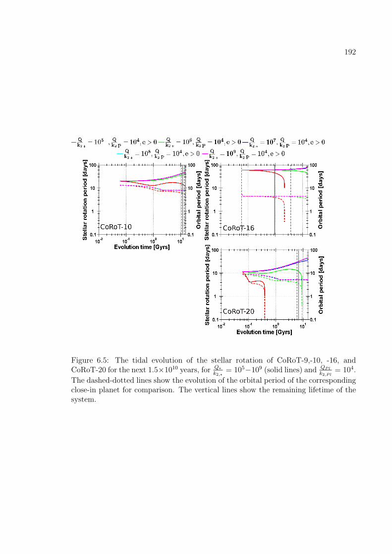
192
Figure 6.5: The tidal evolution of the stellar rotation of CoRoT-9,-10, -16, andCoRoT-20 for the next 1.5×10¹⁰ years, for Q∗
k2,∗= 105−109 (solid lines) and QPl
k2,P l= 104.
The dashed-dotted lines show the evolution of the orbital period of the correspondingclose-in planet for comparison. The vertical lines show the remaining lifetime of thesystem.

193
Stellar rotation evolution of CoRoT-16, QPl
k2,P l= 104
CoRoT-16 experiences tidal spin-up for Q∗k2,∗
≤ 106 as the planet CoRoT-16b moves
toward the star (Figure 5.3) due to stellar tidal friction, just as it was found for
several stars discussed in the previous section. During the first tens of million of
years (Figure 5.4) – when the eccentricity is damped to zero due to planetary tidal
friction – no influence is seen on the stellar rotation. But then again this is expected
because planetary tidal friction only transfers angular momentum within the orbit
and from the planet’s rotation.
Stellar rotation evolution of CoRoT-10, QPl
k2,P l= 104
If Q∗k2,∗
= 106, the rotation of CoRoT-10 is affected - albeit not strongly - by tidal
spin-up although the corresponding orbital migration due to stellar and planetary
tidal friction is small. If Q∗k2,∗
= 105, the spin-up is much stronger due to the positive
feedback effect explained in Section 5.2 that leads to moderate planetary migration.
Stellar rotation evolution of CoRoT-20, QPl
k2,P l= 104
The rotation of CoRoT-20 is already affected for Q∗k2,∗
= 106 by the positive feedback
between stellar and planetary tidal friction, which is to be expected considering the
orbital evolution of CoRoT-20b (Figures 5.3 and 5.4) for small Q∗k2,∗
≤ 106. In the
initial tidal evolution phase, stellar and planetary tidal friction decrease the planet’s
semi major axis and eccentricity more efficiently than each would acting on its own.
Consequently, a comparatively large amount of angular momentum is transferred
from the orbit to the star, which is observed as rapid spin-up already at an early
evolution stage. This is in contrast to the stellar rotation evolution of stars with
close-in planets on circular orbits where the spin-up is the strongest at the end of the

194
tidal evolution. When e has become zero, stellar tidal friction alone is less efficient in
spinning-up the star, but catches up as the planet approaches the star.
For Q∗k2,∗
= 107, the star experiences weak tidal spin-up at the end of the full
evolution time, which is not strong enough to compensate magnetic braking. This
evolution is driven by moderate planetary migration (Figure 5.3) due to stellar tidal
friction. For larger Q∗k2,∗
, the stellar rotation evolution is unaffected.
6.2.1 How does the stellar rotation evolution change withlarger QPl
k2,P l
Now, the tidal evolution scenario for QPl
k2,P l= 104 is compared with tidal evolution
tracks for QPl
k2,P l= 105 and Q∗
k2,∗= 105 − 109 (Figure 6.6), and finally QPl
k2,P l= 106 and
Q∗k2,∗
= 105 − 109 (Figure 6.7)
Stellar rotation evolution of CoRoT-16, QPl
k2,P l= 105 − 106
The stellar rotation evolution of CoRoT-16 does not change when QPl
k2,P lis increased.
Therefore, planetary tidal friction has no influence on the star. The stellar rotation
may only be affected by stellar tidal friction and for the smallest Q∗k2,∗
≤ 106.
6.2.2 Positive feedback effect for planets on orbits withe > 0.5
Stellar rotation evolution of CoRoT-10, QPl
k2,P l= 105 − 106
Comparing the stellar rotation evolution of CoRoT-10 for different QPl
k2,P l-scenarios
shows that for Q∗k2,∗
= 106 the stellar spin-up due to the combination of stellar and
planetary tidal friction becomes stronger with increasing QPl
k2,P l. Still, the stellar rota-
tion period of CoRoT-10 never falls below fifteen days and, at the end of the system’s
lifetime, the stellar rotation period is always larger than 25 days. It would be very

195
Figure 6.6: The tidal evolution of the stellar rotation of CoRoT-9,-10, -16, andCoRoT-20 for the next 1.5×10¹⁰ years, for Q∗
k2,∗= 105−109 (solid lines) and QPl
k2,P l= 105.
The dashed-dotted lines show the evolution of the orbital period of the correspondingclose-in planet for comparison. The vertical lines show the remaining lifetime of thesystem.

196
Figure 6.7: The tidal evolution of the stellar rotation of CoRoT-9,-10, -16, andCoRoT-20 for the next 1.5×10¹⁰ years, for Q∗
k2,∗= 105−109 (solid lines) and QPl
k2,P l= 106.
The dashed-dotted lines show the evolution of the orbital period of the correspondingclose-in planet for comparison. The vertical lines show the remaining lifetime of thesystem.
197
hard to identify such abnormally fast rotating state, especially due the difficulties
when measuring the rotation of a slowly rotating star where error bars can span tens
of days (See Table 1.4).
For Q∗k2,∗
= 105, the combination of stellar and planetary tidal friction acting on
similar timescales affects the stellar rotation more strongly than if stellar tidal friction
would act individually. The combined tidal spin-up is even stronger than magnetic
braking, leading to a net spin-up of the star at an early evolution stage as long as
planetary tidal friction is strong. Apparently, the strength of planetary tidal friction
diminishes over time as the eccentricity approaches zero (Figures 5.8 and 5.10). As
the planet approaches the star, stellar tidal friction eventually becomes stronger than
magnetic braking and is spinning up the star again. If the planet reaches the Roche
limit, which only happens if QP
k2,P≥ 105, the star would rotate with a rotation period
of one day, in the end.
Stellar rotation evolution of CoRoT-20, QPl
k2,P l= 105 − 106
The same feedback effect is also seen in the stellar rotation evolution of CoRoT-20,
if Q∗k2,∗
≤ 106. Indeed, when comparing the rotational evolution of the different QP
k2,P
scenarios, the tidal spin-up due to the combination of stellar and planetary tidal
friction becomes stronger with increasing QPl
k2,P l. But this only holds for the next forty
million years, if Q∗k2,∗
= 105, and for the next one billion years, if Q∗k2,∗
= 106. After
that, magnetic braking takes over as the eccentricity is damped to zero (Figures 5.8
and 5.10). Afterwards, the star may be spun-up again due to stellar tidal friction
alone when the planet enters the Roche zone (Figures 5.7 and 5.9). If CoRoT-20b
enters the Roche zone, the stellar rotation finally ends up with a rotation period of
about one day; regardless of the initial evolution phases and how long it took to

198
reach the Roche zone. Looking at Figures 6.5, 6.6, and 6.7, it appears that the stellar
rotation comes very close to the planetary revolution.
A detailed inspection of Ω∗−n shows that while for QPl
k2,P l= 104 the stellar rotation
always exceeds the planetary revolution (Figure C.5), Ω∗ will be synchronized with
n very briefly for QPl
k2,P l= 104 − 105 (Figures C.6 and C.7). Here, P∗ = 11.5 days
was selected as a start point for the model. It will be shown in Section 8.4.1 and
Chapter F that the CoRoT-20 system may synchronize the stellar rotation with the
planet’s revolution starting with a different initial stellar rotation period within limits
of uncertainties P∗ = 11.5 ± 2.6 days. The system, however, will fail to maintain
a stable double synchronous orbit because magnetic braking removes the required
angular momentum from the system.
6.3 Using stellar rotation as a ’smoking gun’ for
the influence of tidal friction
In this chapter, it was shown for several examples that the stellar rotation is affected
very strongly by tidal friction, even when the orbit remains stable over the remaining
stellar lifetime. Tidal spin-up may be even efficient enough to compensate magnetic
braking. Old stars, in particular, are noticeably affected. Geochronology may yield
false results for the age of a system that once harbored or may still harbor a close-in
massive extrasolar planet.
To gain an insight about what can be learned in terms of Q∗k2,∗
from an abnormally
rotating star, Q∗k2,∗ spin−up limit
is computed for the previously discussed main sequence
stars for which tidal friction may overcome magnetic braking.
For the host stars of planets on circular orbits, mainly the ones described in

199
a) No error bars for the age of the system are given in the detection paper (Bordeet al. (2010))
b) The given age is larger than the estimated total lifetime. Therefore, the system isassumed to be at the end of its lifetime.
System Q∗k2,∗ spin−up limit
age
[Gyrs]CoRoT-1 ≤ 5× 10⁶ -CoRoT-2 ≤ 5× 10⁵ 0.5+3.5
−0.3
CoRoT-7 ≤ 4× 10⁴ 1.7+0.6−0.5
CoRoT-8 ≤ 103 3a
CoRoT-12 ≤ 4× 10⁷ 6.3+3.1−3.1
CoRoT-13 ≤ 105 1.6+1.5−1.5
CoRoT-17 ≤ 2× 10⁷ 10.7+1−1
CoRoT-18 ≤ 2× 10⁶ 0.6+0.4−0.4
Table 6.1: Required Q∗k2,∗
for tidal friction to compensate magnetic braking at the
planet’s current position.
Section 6.1, the following can be found when comparing the tidal friction and magnetic
braking term and solving for Q∗k2,∗
:
dΩtidal friction
dt<
dΩmagnetic braking
dt
Q∗
k2,∗<
3
2
M2Pl
M∗ +MPl
(R∗
a
)3
n2 R2∗
KΩ3∗
(R∗
RSun
)−1/2(M∗
MSun
)1/2
..(6.3.1)
Consequently, Table 6.1 lists the Q∗k2,∗
for which the stellar rotation would be dom-
inated by stellar tidal friction in the near future.
CoRoT-7 and CoRoT-8 are currently not spun up stronger than magnetic braking
can decelerate the star because tidal friction is too inefficient to affect the stellar
rotation for the whole investigated Q∗k2,∗
-range 105 − 109. This is different for the
other stars in the sample: The youngest stars in this sample, CoRoT-2, CoRoT-
13, and CoRoT-18, require Q∗k2,∗
smaller than 105 − 2 × 10⁶. Consequently, only the
smallest investigated Q∗k2,∗
-values are sufficient to spin-up the star at this young age.

200
The oldest stars, CoRoT-12 and CoRoT-17, which are the best indicators for tidal
spin-up, require 4 × 10⁷ and 2 × 10⁷, respectively. Indeed, CoRoT-12 rotates today
(P∗ = 57+∞−28 days) rather slowly showing no indication of considerable spin-up but
rather a rotation period that is expected if the past evolution was dominated by
magnetic braking. Such an evolution requires Q∗k2,∗
= 4 × 10⁷ which agrees nicely
with the limit derived for orbit stability in the previous chapter. CoRoT-17, on the
other hand, appears to be rotating rather fast for a star at the end of its lifetime
(P∗ = 18 ± 2 days), but the rotation period is still larger than 10 days (Figure 6.8).
This may indicate moderate tidal spin-up and planetary migration due to tidal friction
with Q∗k2,∗
≈ 107. CoRoT-1, for which no age constraint is given, requires Q∗k2,∗
less than
5× 10⁶.
Figure 6.8: The stellar rotation periods of the CoRoT-stars of spectral type K andG versus age including the limits of uncertainties. The stellar rotation of CoRoT-17stands out because it is faster than expected for such an old star.
For stars with uncertain magnetic braking efficiency, equation (6.3.1) cannot be

201
used. However, CoRoT-5 is rotating slowly (P∗ = 60+∞−30) and is several billion years
old (Figure 6.9). As was shown in Section 6.1.2, such a star would be spun up
considerably over billion years if Q∗k2,∗
≤ 106. One may therefore tentatively assume
that in this system in the past Q∗k2,∗
≫ 105, because otherwise the star would currently
rotate much faster. When looking at Figure 6.9 one may tentatively assume that
at least the rotations of CoRoT exoplanet host stars of spectral type F seem to
show a deceleration trend with increasing age, hinting to a reduced magnetic braking
scenario.
Figure 6.9: The stellar rotation periods of the spectral type F CoRoT-stars versusage including the limits of uncertainties. The blue crosses are the rotation periodsand the age of CoRoT-3 and CoRoT-15.
For host stars of planets on eccentric orbits, CoRoT-10, CoRoT-16 and CoRoT-20,
Q∗k2,∗ spin−up limit
can be derived, required for tidal friction to spin up the star stronger
than magnetic braking can decelerate it. The tidal stellar rotation evolution of

202
Table 6.2: Required Q∗k2,∗
for tidal friction to compensate magnetic braking for planets
on eccentric orbits at the current position.System Q∗
k2,∗ spin−up limit
QPl
k2,P lage
[Gyrs]CoRoT-9a not affected by tidal friction 104 − 106 0.15− 8CoRoT-10 105.6 104 − 106 2± 1CoRoT-16 2.3× 10⁶ 104 − 106 6.7± 2.8CoRoT-20 106.2 104 − 106 0.1+0.8
−0.04
a) included for completeness.
CoRoT-16 is solely driven by stellar tidal friction after the orbit has become cir-
cular. Therefore, the limiting Q∗k2,∗
can be found by using the equivalent semi major
axis aequiv = 0.063 AU (see previous chapter) and inserting it into equation (6.3.1)
derived for circular orbits.
For CoRoT-10 and CoRoT-20, the stellar rotation evolution depends on stellar
and planetary tidal friction, therefore it depends on the combination of QPl
k2,P land
Q∗k2,∗
if a stellar rotation evolution is dominated by magnetic braking or tidal friction.
The limiting Q∗k2,∗
can be found, however, by the same method by which the orbit
stability limit was found in the previous chapter: by modeling the stellar evolution
for QPl
k2,P l= 104, 105, and 105 and by increasing the stellar tidal dissipation factor –
beginning with Q∗k2,∗
= 105 for CoRoT-10 and Q∗k2,∗
= 106 for CoRoT-20 in each scenario
– until the value is found for which tidal friction spin-up equals magnetic braking.
The results for eccentric orbits are collected in Table 6.2.
Again, stellar spin-up at the current position due to tidal friction is only possible
for very low Q∗k2,∗
= 105 − 106. CoRoT-16’s low stellar rotation (P∗ > 60 days) at
an age of several billion years does not allow for tidal spin-up due to tidal friction.
Consequently, for this system Q∗k2,∗
≫ 105 can be tentatively assumed.

203
6.4 Evaluating evidence for tidal spin up
In summary, it was shown that for slowly rotating host stars of very close-in massive
extrasolar planets considerable spin-up of the stellar rotation is expected when the
planet’s orbit is unstable due to tidal friction. During the migration of the planet
towards the Roche zone, considerable angular momentum is transferred onto the star
whose own angular momentum due to its rotation is in general much smaller than
orbital angular momentum. Furthermore, the amount of angular momentum lost by
magnetic braking is more than compensated by tidal friction. In addition, it was
found that old stars in particular are prone to being spun-up even by moderate tidal
friction.
At last, a limit of Q∗k2,∗
was derived for which the stellar rotation evolution is
dominated by tidal friction between the star and the planet at the current position.
Several old or middle-aged stars, CoRoT-5, CoRoT-12, and CoRoT-16, have been
found which rotate very slowly. This is only feasible if in the past Q∗k2,∗
> 105 − 106.
CoRoT-17, a very old star at the end of its lifetime on the main sequence, may show
moderate tidal spin-up, which would require Q∗k2,∗
≈ 107.
Therefore, it seems implausible that CoRoT planet host stars have very low values
of Q∗k2,∗
= 105−106 requiring an efficient tidal energy dissipation mechanism. Not only
would the orbit of many planets be very unstable (Chapter 5), but the stars would
be tidally spun-up so efficiently that not even magnetic braking would be able to
compensate. Apart from CoRoT-17, no signs of tidal spin-up stronger than magnetic
braking is seen in the CoRoT host stars.
The tidal spin-up of host stars to close-in massive planetary companions may,

204
in addition, affect one method to determine the age of a main sequence star. Gy-
rochronology assumes that main sequence stars rotate slower with increasing age and
that, therefore, the stellar rotation can be used to estimate it’s age. The results de-
rived in this section, however, show that this assumption may not be valid for stars
with close-in massive extrasolar planets. It may not even be valid for stars that don’t
currently have a close-in companion because the stars may have had a planet in the
past that is now lost due to tidal disruption. The only sign of the existence of the
tidally disrupted planet would be the spin-up of the star which may be mistaken
for an indication of young stellar age. The danger of determining a false age by gy-
rochronology is the greatest for old stars. These may be spun up even by moderate
tidal friction i.e. Q∗k2,∗
≈ 108.
6.5 A word regarding the evolution of the tidal
frequencies
The constant Q∗ and QPl model requires the tidal frequencies 2|Ω∗−n| and 2|ΩPl−n|
at least not to vary strongly. This is a valid assumption for CoRoT planetary systems
with circular orbits (Figures C.1, C.2, C.3, C.4) and planets with small to moderate
orbital eccentricties like CoRoT-16b (e ≤ 0.3). The constant Q assumption warrants
further investigation for planets with large orbital eccentricities (e > 0.5) because
|Ω∗ − n|(Figures C.5, C.6, and C.6) and |ΩPl − n| (Chapter D) may vary strongly
during the evolution. It is worthwhile investigating, if the tidal evolution of the
CoRoT-10 and CoRoT-20 system changes for tidal friction models by switching to
the constant τ∗ and τPl formalism, for example, as described in Section 3.1.4. This
shall be reserved for future investigations.

Chapter 7
Tidal evolution of close-inexoplanets around fast rotatingstars
In the systems CoRoT-6 and CoRoT-11, the stars rotate faster than the planets
revolve around them. In contrast to the systems previously discussed this means:
Ω∗ > n (Table 1.4). Consequently, the planets currently migrate outwards and the
stellar rotation is slowed down by tidal friction. Furthermore, it will be found that
a state Ω∗ = n may be reached. Therefore, the orbital and stellar rotation evolution
can not be modeled independent from each other but are closely linked.
Although, the assumption Ω∗ − n ≈ const, in principle, no longer holds all the
time, it will be shown that the synchronicity Ω∗ = n is, in most cases, not achieved by
tidal friction. Furthermore, it will be shown that at least for the CoRoT-11 system,
apart from a brief initial evolution phase, |Ω∗ − n| ≈ const is still a valid assumption
on timescales of billion years.
205

206
The relevant set of equations for modeling the system’s tidal evolution are:
a =sign(Ω∗ − n)3k2,∗MPl
Q∗M∗
(R∗
a
)5
na
Ω∗ =− sign(Ω∗ − n)3k2,∗2I∗Q∗
M2Pl
M∗(M∗ +MPl)
(R∗
a
)3
n2
+dΩ∗
dt m.braking,
where
dΩ∗
dt m.braking= − K
I∗M∗R2∗Ω3
∗
(R∗
RSun
)1/2(M∗
MSun
)−1/2
if Ω∗ < ωsat (7.0.1)
= − K
I∗M∗R2∗Ω2
∗ωsat
(R∗
RSun
)1/2(M∗
MSun
)−1/2
.if Ω∗ > ωsat (7.0.2)
(7.0.3)
Another point of uncertainty is the stellar rotation evolution. CoRoT-6 and
CoRoT-11 are F-stars. Therefore, the evolution of the CoRoT-6 and -11 system
is calculated with full magnetic braking (K = 2.7 × 1040 Nms), reduced magnetic
braking (K = 2.7 × 1039 Nms) and without magnetic braking (K = 0). This yields
three different evolution tracks for the stellar rotation, and for the semi major axes of
the planets. Contrary to the evolution of the planets previously discussed, the orbit
evolution in this chapter depends on when and if the state Ω∗ = n is reached. Luckily,
the stellar rotation period of fast rotating stars has small error bars: P∗ = 7± 1 days
for CoRoT-6 and 1.4 ± 0.3 days for CoRoT-11. Therefore, it is justified to use the
mean value as starting point of the stellar rotation evolution. See also Chapter F
for a model sensitivity analysis that shows that the general evolution will not change
drastically with different start points.
Figure 7.1 shows the evolution of the semi major axes of the planets CoRoT-11b
and CoRoT-6b with full, reduced and no magnetic braking in constant Q∗-formalism.

207
Figure 7.2 shows the corresponding evolution of the stellar rotation of CoRoT-11 and
CoRoT-6.

208
Figure 7.1: The tidal evolution of the semi major axis of the planets CoRoT-6b, and-11b for the next 1.5 × 10¹⁰ years and for Q∗
k2,∗= 105 − 109. The horizontal lines
span the Roche zone. The horizontal line at a = 1R∗ marks the stellar surface. Thevertical lines show the remaining lifetime of the system. See Figure 5.1 for a moredetailed description).

209
Figure 7.2: The tidal evolution of the stellar rotation of CoRoT-6, and -11 for thenext 1.5 × 10¹⁰ years and for Q∗
k2,∗= 105 − 109 (solid lines) with full, reduced and
without magnetic braking. The dashed-dotted lines show the evolution of the orbitalperiod of the corresponding close-in planet for comparison. The vertical lines showthe remaining lifetime of the system.

210
7.1 The tidal evolution of the CoRoT-6 system
The orbit of CoRoT-6b and the stellar rotation of its host star do not change signifi-
cantly under tidal friction for Q∗k2,∗
= 106 − 109. On closer inspection (Figure 7.3), it
becomes apparent that the orbit of CoRoT-6b may change after ten billion years if
Q∗k2,∗
= 105. In contrast to the cases discussed in previous sections, the orbit change
depends on the evolution of the relation Ω∗ − n in the near future which is closely
linked to the stellar rotation evolution (Figure 7.2).
Figure 7.3: The tidal evolution of the semi major axis of the planets CoRoT-6b forthe next 1.5× 10¹⁰ years and for Q∗
k2,∗= 105− 109. The y-axis is this time set to linear
scale and spans from 0.04 to 0.1 AU.

211
Full magnetic braking
For full magnetic braking, the stellar rotation is decelerated within the next three
hundred million years, crosses the Ω∗ − n = 0 state and is decelerated further. The
CoRoT-6 system then becomes a planetary system with a close-in planet around a
slowly rotating star with Ω∗ ≪ n, like the planetary systems discussed previously.
CoRoT-6b will then start to migrate towards the star, but will fail to reach the Roche
limit within the remaining lifetime.
Reduced magnetic braking
For reduced magnetic braking, the planet may migrate slightly away from the star
before the stellar rotation rate is decelerated into a state where again Ω∗ < n. After
that, the planet starts to migrate towards the star after ten billion years. Conse-
quently, the orbit will never near the Roche limit even after fifteen billion years.
No magnetic braking
Without magnetic braking, Ω∗ remains larger than n until tidal friction kicks in and
starts to synchronize the stellar rotation period and the planetary revolution period by
increasing both (See also Figure C.8). The planet will migrate only slightly outwards.
This will be discussed in more detail in Chapter 8.
Summary
Apparently, the early stellar rotation evolution may only be affected by magnetic
braking. Tidal friction may affect the stellar rotation only on longer timescales of
billion of years. Because the tidal friction evolution starts very late into the system’s
evolution time, |Ω∗ − n| ≈ const for the majority of the evolution and, therefore, the

212
constant Q∗ assumption is a valid approach (See also Figure C.8).
In any case, even for Q∗k2,∗
= 105 and for all magnetic braking scenarios, tidal
friction leaves the orbit virtually unchanged and stable during the remaining lifetime.
This confirms the conclusions drawn in Section 4.1, where the semi major axis of
CoRoT-6b a = 0.0855 AU places the planet in the stable region around an F-star for
all investigated Q∗k2,∗
. Only the stellar rotation may be affected significantly within this
time, leading either to a moderate tidal spin-up in the presence of magnetic braking
or to a slight spin-down of the stellar rotation if no magnetic braking is acting on the
star.
7.2 The tidal evolution of the CoRoT-11 system
The CoRoT-11 system, on the other hand, is one system that is expected to evolve
strongly due to tidal friction within the remaining lifetime, as can already inferred
by looking at the tidal stability maps (Section 4.1), the Doodson constant and the
property factor (Section 4.1.1). Here, the close connection between the semi major
axis and the stellar rotation evolution is even more apparent.
Full magnetic braking
In the presence of full magnetic braking acting on the star, the planet hardly has
time to migrate outwards (Figure 7.1). Even for the smallest Q∗k2,∗
the stellar rota-
tion is braked so efficiently that it reaches the state Ω∗ = n within 100 million years
(Figure 7.2). Only for Q∗k2,∗
= 105 will the planet move noticeably outwards in this
brief time. After that, magnetic braking slows down the stellar rotation further. Ap-
parently, the early stellar rotation evolution is dominated again by magnetic braking
and not by tidal friction. Therefore, the planet will start to migrate towards the star

213
again in the long run. apart from the first two hundred million years evolution time,
the tidal evolution of the CoRoT-11 system is similar to the evolution of the CoRoT-
systems with close-in planets around slowly rotating stars discussed in Section 5.1.2
(See also Figure C.8).
Reduced magnetic braking
For reduced magnetic braking acting on the star, the stellar rotation will be faster
than the planet’s revolution only for the the first 600 million years if Q∗k2,∗
≥ 106 and
for the next one billion years if Q∗k2,∗
≥ 105.
During the first evolution stage, while Ω∗ − n > 0 and Q∗k2,∗
≤ 106, the planet will
migrate quite a distance outwards. Indeed, when the state Ω∗ = n is reached, the
distance between the planet and its star is very different for Q∗k2,∗
= 105 − 107, and
Q∗k2,∗
≥ 108.
For Q∗k2,∗
≥ 108, the planet is approximately at the same position as today. If
Q∗k2,∗
= 107, the semi major axis does not change initially but will decrease long after
the stellar rotation has slowed down beyond the Ω∗ = n state. Then, the planet will
migrate towards the star and will even reach the Roche zone within the next seven
billion years. This is, however, longer than the remaining stellar lifetime.
For Q∗k2,∗
= 106, the planet will have migrated noticeably outwards until Ω∗ = n.
After the star is decelerated further by magnetic braking, CoRoT-11b will then start
to migrate towards the star again and will reach the Roche zone within the next two
billion years evolution time; well within the remaining lifetime of the system. For
Q∗k2,∗
= 105 the planet will have migrated even farther outwards until Ω∗ = n. When
the stellar rotation is decelerated further, the planet will again ’turn around’ and
migrate towards the star. It will reach the Roche limit after more than three billion

214
years, much later than compared to the Q∗k2,∗
= 106-evolution track. Figure 7.4 shows
this in more detail.
Figure 7.4: The tidal evolution of the stellar rotation of CoRoT-11 with reducedmagnetic braking for the next three billion years and for Q∗
k2,∗= 105 and 106.
In this detailed view, it is apparent that tidal friction is already efficient enough
during the next hundred million years of evolution time, if Q∗k2,∗
= 105, and that it will
cause a noticeable additional spin-down of the stellar rotation. At the same time, the
planet’s semi major axis and the planet’s revolution period increase considerably due
to tidal friction. The Ω∗ − n = 0 state will be met at 1 billion years, later than for
Q∗k2,∗
≥ 106. For Q∗k2,∗
≥ 106, the stellar rotation evolution is driven mainly by magnetic
braking at this early state and the system will reach Ω∗ − n = 0 after 600 million
years. If Q∗k2,∗
= 105, not only does CoRoT-11b show the strongest outwards migration
compared to larger Q∗k2,∗
-values, it also has more time to migrate outwards. Therefore,
the planet’s semi major axis at the ’turning point’ Ω∗ − n = 0 is so large that tidal
friction is less efficient compared to the Q∗k2,∗
= 106-scenario where the distance at

215
the turning point lies much nearer towards the star. The strength of tidal friction
depends more strongly on the semi major axis a (with the power to five) than on Q∗k2,∗
(linear dependency). This is the only situation found so far where the Q∗k2,∗
= 106-semi
major axis evolution track overtakes the Q∗k2,∗
= 105-semi major axis evolution track
during the planet’s migration towards the star. In any case, the stellar rotation rate
will never match the orbital revolution rate again, even when the planet enters the
Roche zone.
If Q∗k2,∗
≥ 106 the stellar rotation decreases even due to reduced magnetic braking
very fast such that Ω∗ ≪ n before tidal friction can have a noticeable effect on the
system. The constant Q∗ assumption is again valid on timescales of billion of years
on which tidal friction acts. For Q∗k2,∗
= 105, this assumption may be shaky for the first
billion years because tidal spin-up can not be neglected at this early stage. After that,
Ω∗ ≪ n is established and therefore, even in this case, the constant Q∗ assumption
can be assumed as valid at the later evolution phase at least (Figure C.8).
No magnetic braking
If no magnetic braking is acting on the star, the turning point Ω∗ − n = 0 is never
reached and |Ω∗−n| ≈ const (See also Figure C.8). The planet will migrate noticeably
outwards for the whole evolution time if Q∗k2,∗
≤ 107. At the same time, the stellar
rotation is slowed down by a negligible amount due to tidal friction. Even after 15
billion years of evolution and for Q∗k2,∗
= 105, the stellar rotation period changes from
about 1.5 days to 3 days. For higher values of Q∗k2,∗
, tidal friction is too weak to
noticeably affect the system within the next 15 billion years.
216
7.3 Orbital stability
While the orbit of CoRoT-6b is stable within the remaining lifetime, CoRoT-11b may
reach the Roche zone, depending on Q∗k2,∗
and the strength of magnetic braking which
decelerates the stellar rotation.
Without magnetic braking, the planet will never come in the vicinity of the star
for any Q∗k2,∗
. On the contrary, the planet may migrate outwards for small Q∗k2,∗
≤ 107.
The stellar rotation can be regarded as unaltered for any Q∗k2,∗
.
If magnetic braking is decelerating the star, the system will evolve within the
remaining lifetime into a configuration where a close-in extrasolar planet revolves
around a slowly rotating star (Ω∗ ≪ n), like the systems discussed in previous chap-
ters. In consequence, the planet may reach the Roche zone depending on Q∗k2,∗
. For
reduced magnetic braking, it is safe to use the current semi major axis to investigate
orbital stability using equation (5.1.2). For full magnetic braking, equation (5.1.2)
can not be used because the evolution of the semi major axis depends on how far the
planet has migrated during the Ω∗ > n-state. To derive the stability limit, the orbital
evolution is simulated beginning with Q∗k2,∗
= 106 and increasing Q∗k2,∗
in steps of 100.2,
until the evolution track is found for which the planet enters the Roche zone exactly
at the end of the remaining lifetime. The results are listed in Table 7.1.
7.4 Results of the stellar rotation evolution
The fact that stellar rotation is decelerated by even reduced magnetic braking into a
slowly rotating state (Ω∗ ≪ n) shows that fast rotating host stars of close-in extrasolar
planets must either be very young or cannot experience magnetic braking. According
to Barnes (2003), only F stars may meet the last criterion. Furthermore, Bouvier et al.
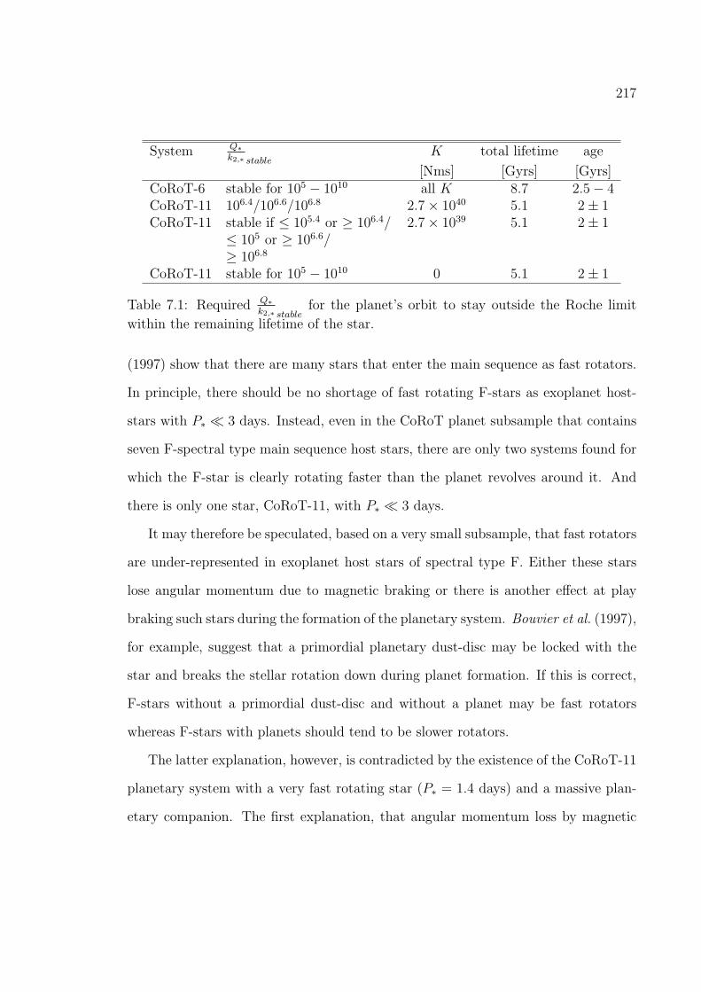
217
System Q∗k2,∗ stable
K total lifetime age
[Nms] [Gyrs] [Gyrs]CoRoT-6 stable for 105 − 1010 all K 8.7 2.5− 4CoRoT-11 106.4/106.6/106.8 2.7× 1040 5.1 2± 1CoRoT-11 stable if ≤ 105.4 or ≥ 106.4/
≤ 105 or ≥ 106.6/≥ 106.8
2.7× 1039 5.1 2± 1
CoRoT-11 stable for 105 − 1010 0 5.1 2± 1
Table 7.1: Required Q∗k2,∗ stable
for the planet’s orbit to stay outside the Roche limit
within the remaining lifetime of the star.
(1997) show that there are many stars that enter the main sequence as fast rotators.
In principle, there should be no shortage of fast rotating F-stars as exoplanet host-
stars with P∗ ≪ 3 days. Instead, even in the CoRoT planet subsample that contains
seven F-spectral type main sequence host stars, there are only two systems found for
which the F-star is clearly rotating faster than the planet revolves around it. And
there is only one star, CoRoT-11, with P∗ ≪ 3 days.
It may therefore be speculated, based on a very small subsample, that fast rotators
are under-represented in exoplanet host stars of spectral type F. Either these stars
lose angular momentum due to magnetic braking or there is another effect at play
braking such stars during the formation of the planetary system. Bouvier et al. (1997),
for example, suggest that a primordial planetary dust-disc may be locked with the
star and breaks the stellar rotation down during planet formation. If this is correct,
F-stars without a primordial dust-disc and without a planet may be fast rotators
whereas F-stars with planets should tend to be slower rotators.
The latter explanation, however, is contradicted by the existence of the CoRoT-11
planetary system with a very fast rotating star (P∗ = 1.4 days) and a massive plan-
etary companion. The first explanation, that angular momentum loss by magnetic

218
braking is at play, is corroborated by the rotation rates and ages of the F-stars found
in the CoRoT-planetary system sample (Figure 6.9). CoRoT-11, the fastest rotation
F-star, is relatively young with an age of 2± 1 billion years. CoRoT-5, the oldest F-
star in this sample with an age of 5−8 billion years, is also the slowest rotating F-star
(P∗ > 30 days). The other F-stars, with ages between one to five billion years show
rotation periods between CoRoT-11’s and CoRoT-5’s. This is exactly the expected
age-rotation period-relation if such stars lose angular momentum due to magnetic
braking. At the same time, the rotation periods of F-stars are at all times - with the
exception of CoRoT-5 - noticeably smaller than that of other main sequence stars.
This would indicate reduced magnetic braking as pointed out by Barnes (2007). As
was shown in this chapter, reduced magnetic braking is sufficient to break the system
out of the Ω∗ > n state.
As a side effect, the investigation of tidal effects within close-in extrasolar systems
may shed light upon the efficiency of magnetic braking in higher mass main sequence
stars.
Furthermore, it was shown that the CoRoT-11 system does not settle at the
Ω∗ − n = 0-state and that the CoRoT-6 system may only settle at Ω∗ − n = 0 in
the absence of magnetic braking and at the end of the remaining lifetime. In the
next chapter, several CoRoT-systems will be investigated that may indeed settle on
a double synchronous state within the remaining stellar lifetime.
Chapter 8
Double synchronous states
The CoRoT-systems CoRoT-3, CoRoT-4 and CoRoT-15 may be in double syn-
chronous rotation (|Ω∗ − n| ≈ 0). CoRoT-6 may evolve into a double synchronous
state in the absence of magnetic braking (see Chapter 7), CoRoT-10 and 20 may
briefly establish a double synchronous state (see Section 6.2). Indeed, in all these
cases (except for CoRoT-10) the planetary revolution rate n is very similar to the
stellar rotation rate Ω∗ (See Section 1.4, Table 1.4). Therefore, the possibility of tidal
equilibrium states warrants in-depth investigation.
8.1 The stability of the double synchronous CoRoT
systems
In the previous chapters it was shown that the evolution of the stellar rotation is driven
by two mechanisms that in most cases counteract each other: Tidal friction decreases
the planet’s orbit and consequently spins up the stellar rotation, in particular for
very small Q∗k2,∗
≈ 105 − 106. Magnetic braking, on the other hand, reduces the stellar
rotation.
While tidal friction is found to be very efficient in spinning up the star, in most
219

220
cases, it is not efficient enough to actually catch up with the planetary revolution rate
n that will usually be larger than the stellar rotation rate Ω∗.
What is the difference between the CoRoT-systems in apparent double synchronous
rotation and other systems? With the exception of CoRoT-4, the main difference lies
in the mass of the companions: CoRoT-3b and CoRoT-15b are the most massive
CoRoT planetary companions (Table 1.3). CoRoT-6b, the planet that may evolve
into a double synchronous rotation at the end of the system’s lifetime, is with a mass
of about 3MJup also relatively massive. The orbits of massive planets and brown
dwarfs should contain more angular momentum than the orbits of the less close-in
Super-Earths, for example.
Indeed, Hut (1980) showed that energy and angular momentum considerations are
necessary to evaluate the stability of double synchronous states. See section 2.9 for
the mathematical derivation.
’Binary systems’ can end up in a double synchronous rotation state only if their
total angular momentum, Ltot, exceeds a critical value Ltot,crit (2.9.10):
Ltot,crit = 4
[G2
27
(I∗M∗R
2∗ + IPlMPlR
2P
) M3∗M
3Pl
M∗ +MPl
]1/4. (8.1.1)
Furthermore, this state can only be stable if the orbital angular momentum, Lorb,
exceeds a critical value Lorb,crit (2.9.14):
Lorb,crit = 3(I∗M∗R
2∗ + IPlMPlR
2∗)n. (8.1.2)
Figure (8.1) shows the total angular momentum of each CoRoT system in comparison
with the total critical angular momentum Ltot,crit and the orbital angular momentum
of each CoRoT planet in comparison with the critical value Lorb,crit.

221
Figure 8.1: Comparison of the total angular momentum, Ltot, of the CoRoT planetswith the critical angular momentum, Ltot,crit, and comparison of the orbital angularmomentum of the CoRoT systems, Lorb, with the critical orbital angular momentumLorb. Top: The ratio Ltot over Ltot,crit for each CoRoT system. Bottom: The ratio ofLorb and Lorb,crit for each CoRoT system.

222
The following eight CoRoT-systems have a total angular momentum which allows
the existence of a double synchronous state: CoRoT-3, CoRoT-4, CoRoT-6, CoRoT-
9, CoRoT-10, CoRoT-11, CoRoT-15 and CoRoT-20. Such a state, however, is only
stable if the orbital angular momenta of the planets exceed the critical value Lorb,crit.
Indeed, CoRoT-4 and CoRoT-11 fail this test. The evolution of CoRoT-11 was
investigated in the previous chapter, and the detailed simulation of the tidal evolution
of this system shows that the Ω∗ = n is only a transient state. In the end, the planet
will migrate towards the host star and may be unstable under tidal friction.
The ’false’ double synchronous case of CoRoT-4
Why are the orbital period of CoRoT-4b and the rotation period of CoRoT-4 al-
most identical, when the CoRoT-4 system fails the angular momentum requirement
for achieving a stable double synchronous state? Furthermore, it was found in Sec-
tion 4.1.1 that the Doodson constant of CoRoT-4b is one of the smallest among the
CoRoT planets. In addition, its orbit is in a region of tidal stability for Q∗k2,∗
= 105−109
when considering the tidal stability map. Therefore, the orbit and stellar rotation
are not expected to be affected strongly within the complete stellar lifetime. Indeed,
the computation of the tidal evolution of the CoRoT-4 system confirms this result
(Figure B.1). Even if a stable double synchronous state would be possible for the
CoRoT-4 system, it is hard to understand how the system should evolve into such
state under tidal friction within its lifetime.
Another explanation is needed for the apparent synchronicity of stellar rotation
and planetary revolution within the CoRoT-4 system: It may just be coincidence
to find a planet around such a star with just about the ’correct’ revolution period.
The stellar rotation of CoRoT-4 of nine days is a typical value for F-stars (See for

223
instance Bouvier et al. (1997) or Barnes (2007)). The stellar rotation is not a very
precisely determined property and therefore might be ’off’ within limits of uncertainty
( P∗ = 9.2+1.7−1.3 days and Porb = 9.20205± 0.00037 days).
’True’ potentially double synchronous systems
The following six CoRoT-systems may end up in a stable double synchronous state
due to angular momentum considerations: CoRoT-3, CoRoT-6, CoRoT-9, CoRoT-10,
CoRoT-15, and CoRoT-20.
CoRoT-6b, however, is relatively far away from its star and was shown to end
up in a double synchronous state very late only in the absence of magnetic braking
and if Q∗k2,∗
= 105 (Chapter 7, Figure 7.2). Interestingly, CoRoT-6b’s semi major axis
(a = 0.0855 AU) is similar to that of CoRoT-4b (a = 0.09 AU), which also orbits an
F-star. But CoRoT-6b (MPl = 2.96MJup) is four times as massive than CoRoT-4
(MPl = 0.72MJup) and, consequently, stellar tidal friction acting in the CoRoT-6
system is four times as efficient than stellar tidal friction acting in the CoRoT-4
system.
CoRoT-9b (a = 0.407 AU) is even farther away from its star and tidal forces
are too weak to force the systems into double synchronous states. Indeed, the stellar
rotation and orbital period are not similar and will not converge within the remaining
lifetime of the systems.
In the end, only four CoRoT-systems remain that may be ’true’ examples of
double synchronous tidal equilibrium states within the lifetime of the star: CoRoT-3,
CoRoT-5, CoRoT-10 and CoRoT-20. These will be discussed in more detail in the
following sections.
The examples of the systems CoRoT-6, and CoRoT-9 illustrate that the energy

224
and angular momentum considerations of Hut (1980) ’only’ allow to draw the conclu-
sion that such systems may end up in principle in stable double synchronous states.
If in reality a double synchronous state is achieved in reasonable time, i.e., within
the lifetime of the system, is another matter entirely that depends on the strength of
stellar tidal friction (and planetary tidal friction for eccentric orbits), and also on the
strength of magnetic braking, in the case of the CoRoT-6 system,.
8.2 Constraints on Q∗k2,∗
to achieve a double syn-
chronous state in the presence of magnetic brak-
ing
To force a star into corotation and to maintain this double synchronous orbit, stellar
tidal friction has to act efficiently. This depends on Q∗k2,∗
. It will be shown that
planetary tidal friction may help to establish a double synchronous state but, in the
long run, planetary tidal friction will not maintain the double synchronous orbit as
the orbital eccentricity is forced rapidly towards zero.
In the following, the evolution of such a system around the double synchronous
rotation state (Ω∗−n ≈ 0 ) is investigated in the presence of at least reduced magnetic
braking.
Several justified assumptions to simplify the calculations are:
• The tidal equilibrium state is stable; that is, the stability criteria discussed in
the previous section are fulfilled.
• The system is assumed to be double synchronous if Ω∗ = n is achieved, because
the planetary rotation is already synchronized with the planets revolution (Sec-
tion 3.2).

225
• Once the system is in double synchronous rotation it remains there.
• The orbit is circular; indeed it will be shown that the potential double syn-
chronous systems either have circular orbits or evolve quickly into circular or-
bits.
• In consequence, the tidal frequency ω = 2|Ω∗ − n| ≈ 0 during the whole calcu-
lation.
• Therefore, the constant Q∗ assumption that requires the tidal frequency or
tidal lag angle to be approximately constant (see Section 2.5), can be used to
investigate the further evolution.
It should be noted, however, that the constantQ∗ required for ω ≈ 0 in this chapter
can, and in fact should, differ from the constant Q∗ required for ω = 2|Ω∗ − n| ≈ 2n
in previous sections for planetary systems with slowly rotating stars where Ω∗ ≪ n.
This should be kept in mind during the discussion of the results.
The systems evolution can be modeled using equations derived in Section 2.6 and
2.10 by:
da
dt= sign (Ω∗ − n)
3k2,∗Q∗
MPl
M∗
(R∗
a
)5
na (8.2.1)
dΩ∗
dt=− sign (Ω∗ − n)
3k2,∗2 ∗ I∗Q∗
M2Pl
M∗(M∗ +MPl)
(R∗
a
)3
n2 (8.2.2)
− K
I∗M∗R∗2Ω3
∗
(R∗
RSun
)1/2(M∗
MSun
)−1/2
.

226
In the following, the constant terms are expressed as follows to simplify the equa-
tions:
A =3k2,∗Q∗
MPl
M∗R5
∗ (8.2.3)
B =3k2,∗
2 ∗ I∗Q∗
M2Pl
M∗(M∗ +MPl)R3
∗ (8.2.4)
C =K
I∗M∗R∗2
(R∗
RSun
)1/2(M∗
MSun
)−1/2
(8.2.5)
B′ =B
G(MPl +M∗)
Then the equations governing the evolution of the system shortly before entering
the doubly synchronous state can be written as:
da
dt= sign (Ω∗ − n)A
n
a4(8.2.6)
dΩ∗
dt= −sign (Ω∗ − n)B
n2
a3− CΩ3
∗ (8.2.7)
= −sign (Ω∗ − n)B′n4 − CΩ3∗, (8.2.8)
where in addition Kepler’s third law a3 = G(M∗ +MPl)/n2 is used to express the
equation describing Ω∗ in terms of n and Ω∗ instead of a, n and Ω∗.
Furthermore, it is advisable to describe the situation with respect to the fictive
double synchronous orbit for any given Ω∗ (Figure 8.2). This is the orbit for which
the mean motion is exactly n = Ω∗. If the planet is revolving faster around the star
than the star rotates about its axis of symmetry, n > Ω∗, and the planet’s orbit
would lie inside the synchronous orbit. After all, a3 = G(M∗ +MPl)/n2 according
to Kepler’s law. Such a configuration is sometimes called a subsynchronous orbit in
the literature (Lanza (2010) and Levrard et al. (2009), for example). If n < Ω∗, the
planet’s orbit lies outside the double synchronous orbit.

227
Figure 8.2: The orbit of a planet around a star with respect to the double synchronousorbit (n = Ω∗, solid line). If n < Ω∗, the orbit lies outside the double synchronousorbit (dashed line). If n > Ω∗, the orbit lies inside the double synchronous orbit(dotted line)
In the following, the evolution into and around the double synchronous state is
investigated in several steps:
Step 0: One time step before double synchronicity As a start point of inves-
tigation, a situation was chosen where the star rotates slower (Ω∗,0) than a
close-in planet with semi major axis a0 and mean motion n0 revolves around it.
Consequently, Ω∗,0 < n0 shortly before entering double synchronous rotation.
The orbit lies inside the double synchronous orbit for which ndoub,0 = Ω∗,0.
228
This initial situation is selected because it is more difficult to achieve the double
synchronous state from inside the double synchronous orbit: tidal friction spins
up the star and forces the star and planet into corotation. Magnetic braking, on
the other hand, decelerates the star away from the double synchronous rotation
state1. Therefore sign (Ω∗ − n) = −1. In this case, the following set of equations
describe the evolution of the system under stellar tidal friction:
da
dt= −An0
a40(8.2.9)
dΩ∗
dt= B′n4
0 − CΩ3∗,0. (8.2.10)
Step 1: Double synchronous orbit achieved After a time step δt, the semi ma-
jor axis a1 and stellar rotation rate Ω∗,1 are:
a1 = a0 +da
dtδt
Ω∗,1 = Ω∗,0 +dΩ∗
dtδt.
or
a1 = a0 − An0
a40δt
Ω∗,1 = Ω∗,0 + (B′n40 − CΩ3
∗,0)δt.
This new orbit should be double synchronous: Ω∗,1 = n1 = ndoub,1, with n1 =√G(MPl +M∗)/a31. This is shown in Figure 8.3. The new planetary orbit is
1If Ω∗,0 > n0 is chosen as initial situation, both, magnetic braking and tidal friction, woulddecelerate the stellar rotation. From this starting point, the double synchronous state is easier toachieve.
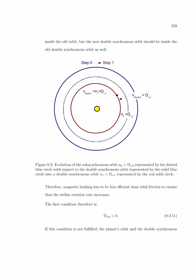
229
inside the old orbit, but the new double synchronous orbit should be inside the
old double synchronous orbit as well.
Figure 8.3: Evolution of the subsynchronous orbit n0 > Ω∗,0 represented by the dottedblue circle with respect to the double synchronous orbit represented by the solid bluecircle into a double synchronous orbit n1 = Ω∗,1 represented by the red solid circle.
Therefore, magnetic braking has to be less efficient than tidal friction to ensure
that the stellar rotation rate increases.
The first condition therefore is:
Ω∗,0 > 0. (8.2.11)
If this condition is not fulfilled, the planet’s orbit and the double synchronous

230
orbit will evolve away from each other (Figure 8.4).
The condition above can also be expressed as:
B′n40 − CΩ3
∗,0 > 0. (8.2.12)
It is at this point safe to assume that n0 and Ω∗,0 are already very similar just
before entering the double synchronous state: n0 ≈ Ω∗,0. Therefore the relation
above reduces to
B′n0 > C. (8.2.13)
Or fully expressed and solved for Q∗k2,∗
:
3k2,∗2I∗Q∗
M2Pl
GM∗(MPl +M∗)2R3
∗n0 >K
I∗M∗R2∗
(R∗
RSun
)1/2(M∗
MSun
)−1/2
(8.2.14)
3
2
k2,∗Q∗
M2Pl
G(MPl +M∗)2R5
∗n0 > K
(R∗
RSun
)1/2(M∗
MSun
)−1/2
(8.2.15)
Q∗
k2,∗< n0
3
2
M2Pl
G(MPl +M∗)2R5
∗1
K
(R∗
RSun
)−1/2(M∗
MSun
)1/2
(8.2.16)
This is the upper limit of Q∗k2,∗
required to force a planetary system in double
synchronous rotation despite magnetic braking. It depends on the planetary
revolution rate n or on a−3/2 (using Kepler’s third law). The larger the semi
major axis and the lower n is, the lower is the required Q∗k2,∗
for establishing
double synchronous rotation.
Up to now, it was only made sure that the double synchronous orbit decreases
as well as the planet’s orbit. Close inspection of Figure 8.3 makes another

231
Figure 8.4: Evolution of a subsynchronous orbit n0 > Ω∗,0 represented by the dottedblue circle with respect to the double synchronous orbit represented by the solid bluecircle if magnetic braking is more efficient than tidal friction. In the next time step, theplanet’s orbit would shrink (dotted red circle) but the stellar rotation would decreaseand lead to a double synchronous orbit with even larger radius, where n1 = Ω∗,1,represented by the red solid circle.
232
condition apparent: The double synchronous orbit must decrease faster than
the planet’s orbit for the two to meet.
ndoub,0 = Ω∗,0 > n0. (8.2.17)
If C = 0, that is, if no magnetic braking is counteracting tidal friction, equa-
tion (8.2.17) is equivalent to equation (8.1.2). This is proven in detail in Chap-
ter G2. Without magnetic braking, therefore the system has no problem to
achieve a double synchronous state, as long as the orbital angular momentum
exceeds the critical value Lorb,crit.
If C > 0, the orbital angular momentum has not only to exceed Lorb,crit but
the sum of Lorb,crit + ∆Lmagnetic braking , where ∆Lmagnetic braking is the total an-
gular momentum that magnetic braking removes from the system during the
stellar lifetime. Incidently, in a subsequent section there will be investigated a
CoRoT system that fulfills the requirement Lorb > Lorb,crit but fails the stronger
requirement Lorb > Lorb,crit +∆Lmagnetic braking .
In summary, two requirements were identified that must be fulfilled to achieve
a double synchronous state even in the presence of magnetic braking. Q∗k2,∗
must be
lower than the upper limit defined by 8.2.16. In addition to the requirements given in
the previous section for the orbital and total angular momentum (equations (8.1.1)
and (8.1.2)), the orbital angular momentum has to exceed: Lorb,crit+∆Lmagnetic braking
to achieve a double synchronous state.
Whether the system ends up in a double synchronous state in reasonable time - on
time scales of several billion years - is another matter entirely and will be investigated
in a subsequent section.
2It should be noted that this proof is original work and not adopted from other authors.

233
8.3 Long-term stability of double synchronous or-
bits in the presence of magnetic braking
Can tidal interactions maintain this state in the future despite magnetic braking,
once the double rotation state is established? To answer this question, the evolution
of the system is investigated starting with the system in double synchronous rotation
(Figure 8.5):
Step 2 The system’s parameters at this point are:
a1 = (G(MPl +M∗)/n21)
1/3
Ω∗,1 = n1.
Therefore, from equations 8.2.6 and 8.2.8 the following set of equations govern
the further evolution:
da
dt 1= 0
dΩ∗
dt 1= −Cn3
1.
In the presence of magnetic braking, Ω∗ always decreases once the system is
in a double synchronous state. This is the same as stating that the double
synchronous orbit is forced outside of the the planet’s orbit by magnetic braking.
Step 3 = Step 0 The system is in the following configuration
a2 = a1
Ω∗,2 > Ω∗,1 = n1.
The system is again in a subsynchronous rotation state as described in the
previous section as ’step 0’ and depicted in Figure 8.3.

234
Figure 8.5: Evolution of double synchronous orbit n1 = Ω∗,1 represented by the solidblue circle in the presence of magnetic braking. The stellar rotation becomes slowerand as a consequence the radius of the new double synchronous orbit is larger thanthe radius of the previous one (solid red circle), while the planet’s orbit (dotted redcircle) remains at its position. This is the same situation than depicted in Figure 8.3.
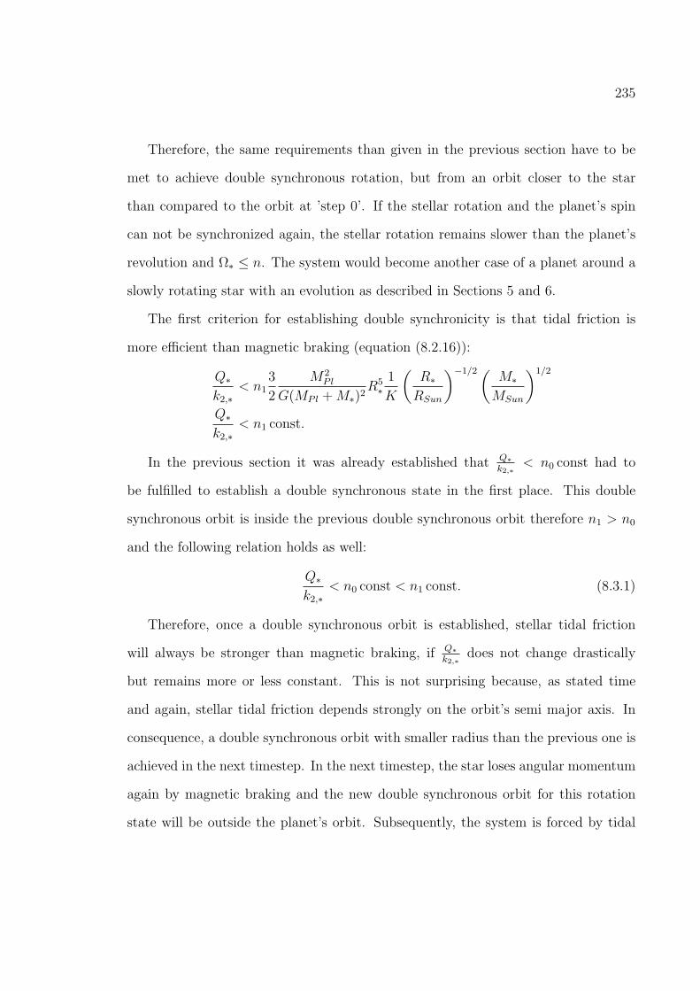
235
Therefore, the same requirements than given in the previous section have to be
met to achieve double synchronous rotation, but from an orbit closer to the star
than compared to the orbit at ’step 0’. If the stellar rotation and the planet’s spin
can not be synchronized again, the stellar rotation remains slower than the planet’s
revolution and Ω∗ ≤ n. The system would become another case of a planet around a
slowly rotating star with an evolution as described in Sections 5 and 6.
The first criterion for establishing double synchronicity is that tidal friction is
more efficient than magnetic braking (equation (8.2.16)):
Q∗
k2,∗< n1
3
2
M2Pl
G(MPl +M∗)2R5
∗1
K
(R∗
RSun
)−1/2(M∗
MSun
)1/2
Q∗
k2,∗< n1 const.
In the previous section it was already established that Q∗k2,∗
< n0 const had to
be fulfilled to establish a double synchronous state in the first place. This double
synchronous orbit is inside the previous double synchronous orbit therefore n1 > n0
and the following relation holds as well:
Q∗
k2,∗< n0 const < n1 const. (8.3.1)
Therefore, once a double synchronous orbit is established, stellar tidal friction
will always be stronger than magnetic braking, if Q∗k2,∗
does not change drastically
but remains more or less constant. This is not surprising because, as stated time
and again, stellar tidal friction depends strongly on the orbit’s semi major axis. In
consequence, a double synchronous orbit with smaller radius than the previous one is
achieved in the next timestep. In the next timestep, the star loses angular momentum
again by magnetic braking and the new double synchronous orbit for this rotation
state will be outside the planet’s orbit. Subsequently, the system is forced by tidal

236
friction on a double synchronous orbit with an even smaller radius and so forth and
so forth (Figure 8.6).
This creates the strange situation of a system in or near double synchronous ro-
tation which is not stable. The orbit still decays as the stellar rotation is ’dragged
along’ and always kept close to the orbital mean motion. Therefore, a planetary sys-
tem cannot be regarded as tidally stable if Ω∗ ≈ n, unless stellar angular momentum
loss by magnetic braking is investigated.
Another point of concern is that the system loses orbital angular momentum as
well as the double synchronous orbit decays, therefore Lorb > Lorb,crit+∆Lmagnetic braking
may at one point not be fulfilled anymore as the double synchronous orbit moves
closer and closer to the star. Should that happen, synchronicity can not be reestab-
lished again and the double synchronous orbit will lag behind the planet’s orbit: the
planetary system will become unstable.
In any case, in the presence of magnetic braking a double synchronous orbit may
be unstable.
8.3.1 The possible decay of the double synchronous orbit dueto magnetic braking
A step-wise calculation of the decay of the double synchronous orbit as described
above would be very cumbersome and computationally challenging. In the following,
it will be investigated how this can be achieved more efficiently.
The key to a better description is again the angular momentum:
Step 1 The system is in double synchronous rotation. The total angular momentum
of a double synchronous system can be expressed in terms of orbital revolution
rate ndoub,1. Because Ω∗,1 = n1 and Kepler’s third law is used to replace a1 with

237
Figure 8.6: The decay of a double synchronous orbit (red circles) in the presence ofmagnetic braking starting with a subsynchronous planetary orbit (the blue dottedcircle is the planet’s orbit, the blue solid line is the ’fictive’ double synchronous orbitthat lies outside the planet’s orbit). In the first step, the planetary and double syn-chronous orbit converge to a new double synchronous orbit with smaller radius(red).In the next step, the stellar rotation decreases and for this state the ’fictive’ doublesynchronous orbit (blue) would lie outside the ’old’ double synchronous state wherethe planet is still orbiting the star. In the next step, the planet’s and double syn-chronous orbit converge into a new double synchronous orbit with even smaller radiusetc. In consequence, the planetary orbit continually shrinks. The double synchronousorbit alternatively shrinks and expands, as indicated by the black arrows.

238
n1 = ndoub,1:
L1 = Ltot = I∗M∗R2∗ndoub,1 +
MPlM∗
MPl +M∗µ2/3n
−1/3doub,1, (8.3.2)
where µ = G(MPl +M∗).
Step 2 The star loses angular momentum δL1 due to magnetic braking according to
equation (2.10.4):
L2 = L1 − δL1 = I∗M∗R2∗Ω∗,2 +
MPlM∗
MPl +M∗µ2/3n
−1/32 , (8.3.3)
where Ω∗,2 < n2 and n2 = n1 = ndoub,1 as explained in the previous section.
Step 3 Now tidal friction acts to synchronize the stellar rotation and orbital revolu-
tion rate again, but only if tidal friction is more efficient than magnetic braking
(Ωmag.braking < Ωtidalfriction). This is a condition that may safely be regarded as
fulfilled as was proven in previous sections (equation 8.2.11). This is equivalent
to saying that from the point of view of magnetic braking, tidal friction acts
’instantly’ to reestablish a new double synchronous state. Therefore, there will
only be a transfer of angular momentum from the orbit to the star during the
synchronization:
L3 ≈ L2 = I∗M∗R2∗ndoub,2 +
MPlM∗
MPl +M∗µ2/3n
−1/3doub,2. (8.3.4)
The system will settle again on a new double synchronous orbit that lies beneath
the previous one (ndoub,2 < ndoub,1).
Because the total amount of angular momentum loss does not change from step
2 to step 3, the amount of angular momentum lost by magnetic braking can be

239
calculated using equation (2.10.4). The equation only depends on constants and
ndoub,1. Therefore, the new double synchronous rotation rate ndouble,2 can be calculated
by going from step 0 directly to step 2.
Therefore, the decay of the double synchronous orbit in the presence of magnetic
braking can be modeled using equation 2.10.4 and setting it equal to dLtot
dt:
dJ
dt= I∗M∗R
2∗ndoub +
MPlM∗
MPl +M∗µ2/31
3n−4/3doub ndoub. (8.3.5)
Solving for ndoub gives:
dndoub
dt=
dΩ∗
dt=
dJdt
C∗ +Bn−4/3doub
, (8.3.6)
where C∗ = I∗M∗R2∗ is the stellar moment of inertia and B = 1
3MPlM∗MPl+M∗
µ2/3.
As a reminder, the angular momentum loss due to magnetic braking, dJdt, is once
again shown at full length:
dJ
dt Ω∗=−KΩ3
∗
(R∗
RSun
)0.5(M∗
MSun
)−0.5
for Ω∗ < ωsat (8.3.7)
dJ
dt Ω∗=−KΩ∗ω
2sat
(R∗
RSun
)0.5(M∗
MSun
)−0.5
for Ω∗ ≥ ωsat,
where K is the phenomenologically derived scaling constant (K = 2.7× 1040 Nms
for low-mass main sequence stars).
Using equation (8.3.6), the evolution of the systems CoRoT-3 and CoRoT-15 can
be calculated (Figures 8.7 and 8.8), as long as the orbital and total angular momentum
fulfill equations (8.1.2) and (8.1.1).
240
8.4 Tidal evolution of the CoRoT-3 and CoRoT-15
system
The tidal evolution of CoRoT-3 and CoRoT-15 systems are modeled using Equa-
tions (5.1.1) and (6.1.1), as long as Ω∗ < n. To account for the uncertainty in mag-
netic braking in the F-stars CoRoT-3 and CoRoT-15, the semi major axis and stellar
rotation evolution is simulated with full, reduced and without magnetic braking (See
also Section 5.1.2) by using different scaling factors K:
• K = 2.7×1040 Nms for ’full magnetic braking’, adopting the same scaling factor
as for low mass main sequence stars,
• K = 2.7× 1039 Nms for ’reduced magnetic braking’,
• K = 0 for a model without magnetic braking.
As soon as a state Ω∗ = n is reached, the further evolution is modeled using
Equation 8.3.6 as a ’short cut’ saving computation time.
Figures 8.7 and 8.8 show the evolution of the planet’s orbit and the stellar rotation
for the next 15 billion years. Figures 8.9 and 8.10 show a close-up of the first billion
years of evolution. This allows to better identify the conditions for which the CoRoT-
3 and CoRoT-15 system may enter the double synchronous state.(See also Figures C.9
for the Ω∗−n evolution). The evolution was modeled with the average stellar rotation
period as given in Table 1.4. It should be considered that a variation of the stellar
rotation period at the start of the computations may change the semi major axis and
stellar rotation evolution because the Ω∗ = n state may be met earlier or later than
computed here. This does not affect, however, the qualitative results derived in terms
of magnetic braking and Q∗k2,∗
(See also Chapter F).

241
Figure 8.7: The tidal evolution of the semi major axis of the brown dwarfs CoRoT-3b,and -15b for the next 1.5× 10¹⁰ years and for Q∗
k2,∗= 105 − 109. The horizontal lines
span the Roche zone. The horizontal line at a = 1R∗ marks the stellar surface. Thevertical lines show the remaining lifetime of the system.

242
Figure 8.8: The tidal evolution of the stellar rotation of CoRoT-3, and -15 for thenext 1.5 × 10¹⁰ years and for Q∗
k2,∗= 105 − 109 (solid lines) with full, reduced and
without magnetic braking. The dashed-dotted lines show the evolution of the orbitalperiod of the corresponding close-in planet for comparison. The vertical lines showthe remaining lifetime of the system.
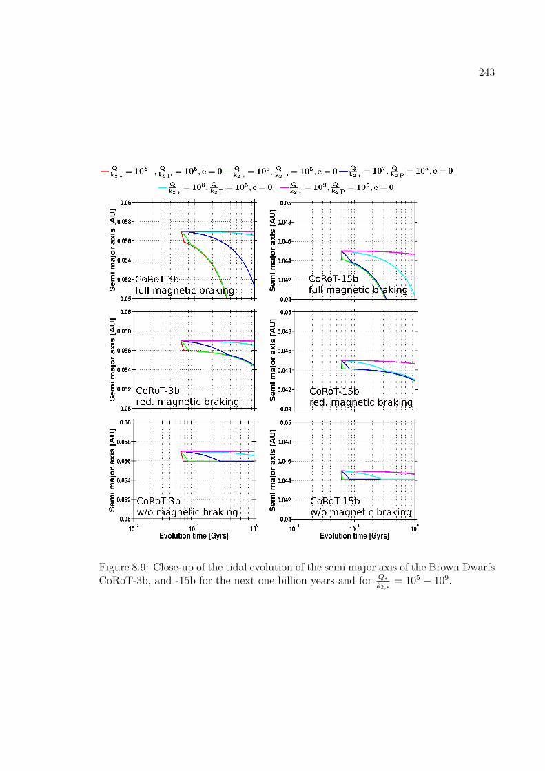
243
Figure 8.9: Close-up of the tidal evolution of the semi major axis of the Brown DwarfsCoRoT-3b, and -15b for the next one billion years and for Q∗
k2,∗= 105 − 109.

244
Figure 8.10: Close-up of the tidal evolution of the stellar rotation of CoRoT-3, and-15 for the next one billion years and for Q∗
k2,∗= 105−109 (solid lines) with full, reduced
and without magnetic braking. The dashed-dotted lines show the evolution of theorbital period of the corresponding close-in planet for comparison.

245
The CoRoT-3 system, full magnetic braking
With full magnetic braking, the CoRoT-3-system will not reach the double syn-
chronous state if Q∗k2,∗
≥ 108, although the system is near the double synchronous
Ω∗ = n state and although the system in principle fulfills the energy and angular
momentum criteria for a stable double synchronous state. But magnetic braking is
stronger than tidal friction and slows the stellar rotation efficiently away from the
near-double synchronous state. For Q∗k2,∗
= 108, tidal friction appears to catch up in
strength with magnetic braking after several billion years and begins to dominate the
stellar rotation and semi major axis evolution. But even then it will not come near
the double synchronous state at the end of the evolution time, that is, after 15 billion
years. If Q∗k2,∗
= 107, tidal friction will ’win’ after two billion years and force the system
in double synchronous rotation. After that, the system will continue to lose angular
momentum due to magnetic braking. As a consequence, the double synchronous or-
bit will decay and will even reach the Roche limit very quickly one hundred million
years later. In principle, the orbit is already on its way towards the Roche limit when
stellar rotation catches up with the planet’s revolution rate.
If Q∗k2,∗
≤ 106, the double synchronous state will be reached within the next few ten
million years. After that, the double synchronous orbit will decay. As shown in the
section above, once inside the double synchronous state, the decay will not depend
on Q∗k2,∗
but only on the strength of magnetic braking and the revolution rate of the
double synchronous orbit ndoub. Because the double synchronous revolution rate that
is reached for Q∗k2,∗
= 105 and Q∗k2,∗
= 106 is almost the same, the further evolution is
virtually the same for both Q∗k2,∗
-values.

246
The CoRoT-3 system, reduced magnetic braking
With reduced magnetic braking, the system will reach the double synchronous state
already after a few hundred million years for Q∗k2,∗
≤ 107. The evolution of this double
synchronous state is same for very Q∗k2,∗
≤ 107. Consequently, the decay of the double
synchronous orbit will be identical. The decay will take, however, longer than for full
magnetic braking. The orbit will reach the Roche zone after ca. six billion years. For
Q∗k2,∗
≥ 108, even for reduced magnetic braking, tidal friction is still not strong enough
to force the system into corotation.
The CoRoT-3 system, no magnetic braking
In the absence of magnetic braking, the orbit will not decrease any further once the
double synchronous state is reached (Figure 8.11). That will happen within the next
ten million years if Q∗k2,∗
= 105, the next twenty million years if Q∗k2,∗
= 106, within
the next two hundred million years if Q∗k2,∗
= 107 and ca. after two billion years if
Q∗k2,∗
= 108. Even for Q∗k2,∗
= 109 the system may gradually evolve towards the double
synchronous state over billions of years, but not quite reach it after 15 billion years.
The CoRoT-15 system, full magnetic braking
The CoRoT-15 system will evolve into a double synchronous state within the next
few ten million years if Q∗k2,∗
≤ 107 in the presence of full magnetic braking. Even for
Q∗k2,∗
= 108 the system will be in double synchronous rotation after two billion years.
For Q∗k2,∗
= 109, tidal friction will have compensated magnetic braking after three
billion years and spin-up the star. The system will not reach the double synchronous
state, however, within the evolution time of 15 billion years.

247
Figure 8.11: Close-up of the tidal evolution of the semi major axis of the BrownDwarfs CoRoT-3b for the next 15 billion years and Q∗
k2,∗= 105 − 109. Vertical lines
denote the minimum, average and maximum remaining lifetime.
The CoRoT-15 system, reduced magnetic braking
In the presence of reduced magnetic braking the system will still evolve very fast
(within the next few ten million years) towards the double synchronous state if Q∗k2,∗
≤
107. For Q∗k2,∗
= 108, the system will be caught within the next few hundred million
years in a double synchronous state already. The subsequent decay of the double
synchronous orbit, on the other hand, will take much longer than with full magnetic
braking. The orbit may reach the Roche zone after ca. eight billion years, which is
probably longer than the remaining lifetime. Indeed, within the remaining lifetime,
the double synchronous orbit will only migrate moderately. If Q∗k2,∗
= 109, the system
will hardly evolve. A slow evolution towards a double synchronous state can be seen
after eight billion years. The system, however, will not have reached the double

248
synchronous state at the end of the simulation time.
The CoRoT-15 system, no magnetic braking
Without magnetic braking, the system will still evolve within a few ten million years
towards the double synchronous state for Q∗k2,∗
≤ 107. Apparently, tidal friction is
so efficient for these Q∗k2,∗
-values that magnetic braking hardly changes anything. If
Q∗k2,∗
= 108, the system may be a little earlier in a double synchronous state than with
reduced magnetic braking. The difference is, however, negligible. If Q∗k2,∗
= 109, the
system may reach the double synchronous state as well and even within the remaining
lifetime of the star. Once the system is in double synchronous rotation, it will stay
there and will not evolve further. As was shown in Section 2.9, the double synchronous
state is stable if the angular and energy criteria are fulfilled.
Summary of the results of the CoRoT-3 and CoRoT-15 evolution
The lessons learned from these scenarios are:
a Only relatively massive substellar companions i.e. Brown Dwarfs on close orbit are
capable to spin-up the star sufficiently within the remaining lifetime of the star
to achieve a double synchronous state from state Ω∗ < n.
b To achieve a double synchronous state within the remaining lifetime Q∗k2,∗
≤ 107 for
the CoRoT-3 system, and Q∗k2,∗
≤ 108 for the CoRoT-15 system is required.
c If the system has been forced by tidal friction into a double synchronous state, the
double synchronous orbit will decay in the presence of magnetic braking, in any
case, and may even reach the Roche limit within the remaining lifetime for full
magnetic braking.

249
d The orbital decay may take several billion years for reduced magnetic braking,
which is, however, too long to lead to significant decay within the remaining
stellar lifetime. Therefore, the double synchronous orbits of CoRoT-3b and
CoRoT-15b can be regarded as stable in the reduced magnetic braking scenario.
e Without magnetic braking, a double synchronous system will be stable and the
planet will be ’safe’ from migrating towards the star. Furthermore, a rather
massive companion (MPl ≈ 60MJup) like CoRoT-15b will evolve within the
remaining stellar lifetime into a double synchronous state for every Q∗k2,∗
= 105−
109.
f In any case, a double synchronous orbit is more stable than the ’normal’ non-
synchronous orbit if Q∗k2,∗
≤ 106. Even in the presence of full magnetic braking,
the decay rate of the double synchronous orbit is much smaller than the decay
rate of the non-synchronous planetary orbit if Q∗k2,∗
≤ 106.
8.4.1 Why will CoRoT-20 not be able to maintain a stabledouble synchronous state?
In section 2.9, the CoRoT-20 system was identified as one of three systems that may
end up in a stable double synchronous state configuration. Its tidal evolution was
already investigated in Sections 5.2 and 6.2 as an example of a potentially unstable
system where the planet may reach the Roche zone within the lifetime of the start.
Figures C.6 and C.7 suggest that for Q∗k2,∗
= 105 and QPl
k2,P l≥ 105, the CoRoT-20
system may come very close to Ω∗ = n at an evolution time of 90 million years for
a very brief time. Still, it can safely be concluded that the system never settles at a
double synchronous orbit.

250
Decay of total angular momentum by magnetic braking
This can be explained by looking in more detail into the angular momentum evolution.
The system’s total angular momentum currently exceeds the critical value, but only
barely (Figure 8.1).
The critical total angular momentum, Ltot,crit, for the CoRoT-20 system is:
Ltot,crit = 4
[G2
27
(I∗M∗R
2∗ + IPlMPR
2Pl
) M3∗M
3Pl
M∗ +MPl
]1/4= 9.74× 1042kg
m2
s. (8.4.1)
Currently, the total angular momentum, Ltot of the CoRoT-30 system is the sum of
the orbital angular momentum and the angular momenta of the rotation of CoRoT-20
and CoRoT-20b:
Ltot = Lorb + Lrot,P l + Lrot,∗
=MPlM∗
MPlM∗n2a
√1− e2 +MPl ·R2
Pl · IPlΩPl +M∗ +R2∗ ∗ I∗Ω∗
=[9.5× 1042 + 1.5× 1038 + 5.05× 1041
]kg
m2
s
= 1× 1043kgm2
s(8.4.2)
It was confirmed again that, even for rather massive exoplanets, the angular mo-
mentum of the planet’s rotation is negligible. More importantly is the following result:
The total angular momentum of the CoRoT-20 system is only slightly larger than the
critical total angular momentum to begin with.
In the next few billion years, the system loses angular momentum by magnetic

251
braking. The angular momentum loss rate is currently (Section 2.10):
dJ
dt= −KΩ3
∗
(R∗
RSun
)1/2(M∗
MSun
)−1/2
= −7.23× 1024kgm2
s2. (8.4.3)
This value can be used to roughly estimate the angular momentum loss in the
next one billion years by assuming that dJdt
is more or less constant over this time
period ∆t = 1 Gyrs:
∆J =dJ
dt×∆t
= −2.3× 1041kgm2
s. (8.4.4)
As can be seen, when subtracting ∆J from Ltot, the system has already lost so
much angular momentum after one billion years that Ltot ≈ Ltot,crit. Because the
star continues to lose angular momentum, the system is expected to have a total
angular momentum Ltot smaller than Ltot,crit after more than one billion years. As
Hut (1980) has shown, a double synchronous state is not possible in such a case. This
is, however, only a quick ’back of the envelope’ calculation. Figure 8.12 shows the
evolution of the total angular momentum for magnetic braking and tidal friction with
QP
k2,P= 105 and Q∗
k2,∗= 106 as modeled in Sections 5.2 and ??. As can be seen, the
total angular momentum decreases due to magnetic braking and falls below Ltot,crit
even earlier than estimated above. After 600 hundred million years already, the total
angular momentum does not exceed Ltot,crit anymore, which is the prerequisite for a
double synchronous state.

252
0 1 2 3 4 5 60
0.5
1
1.5
2
evolution time [Gyrs]
Figure 8.12: The evolution of the ratio of total angular momentum Ltot over criticaltotal angular momentum Ltot,crit for the CoRoT-20 system under tidal friction andmagnetic braking with QPl
k2,P l= 105 and Q∗
k2,∗= 106. The horizontal dashed line marks
Lcrit,tot.
Alternative evolution of the CoRoT-20 system with P∗ = 8.9 days
In Sections 5.2 and 6.2, however, P∗ = 11.5 days was selected as initial condition
for the tidal evolution (Ω∗ < n). It was already stated there that the limits of
uncertainties of the stellar rotation P∗ = 11.5 ± 2.6 days allow also for an evolution
with Ω∗ = n, and Ω∗ > n.
In the following, tidal evolution tracks of the CoRoT-20 system using P∗ = 8.9 days
as initial condition are discussed, with Q∗k2,∗
= 105 − 109 and QPl
k2,P l= 104 − 106
(Figures 8.13, 8.14, and 8.15). The evolution tracks were calculated using Equa-
tions (5.2.1), (5.2.2), (5.2.3), and (5.2.4) (See Section 5.2).

253
Figure 8.13: Tidal evolution of the CoRoT-20 system with P∗ = 8.9 days as initialcondition of the stellar rotation. The panels show the evolution of the semi majoraxis, the eccentricity, the stellar rotation (solid lines) and planetary orbital revolutionperiod (dashed lines), and of |Ω∗−n| for Q∗
k2,∗= 105−109 and QPl
k2,P l= 104. The vertical
lines show the remaining stellar lifetime with limits of uncertainty.
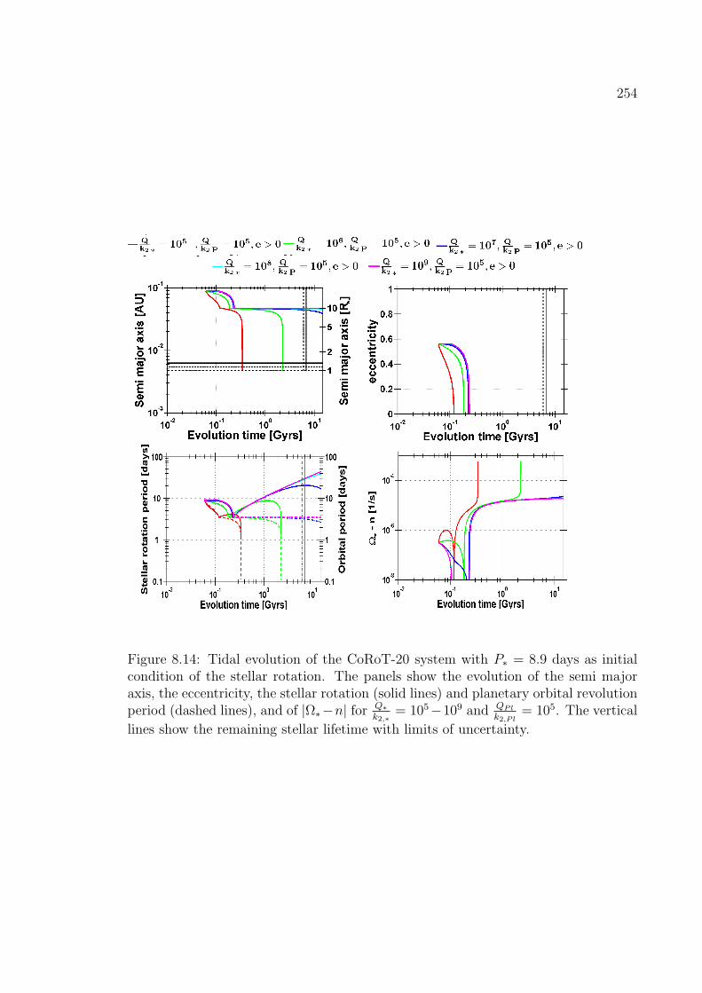
254
Figure 8.14: Tidal evolution of the CoRoT-20 system with P∗ = 8.9 days as initialcondition of the stellar rotation. The panels show the evolution of the semi majoraxis, the eccentricity, the stellar rotation (solid lines) and planetary orbital revolutionperiod (dashed lines), and of |Ω∗−n| for Q∗
k2,∗= 105−109 and QPl
k2,P l= 105. The vertical
lines show the remaining stellar lifetime with limits of uncertainty.
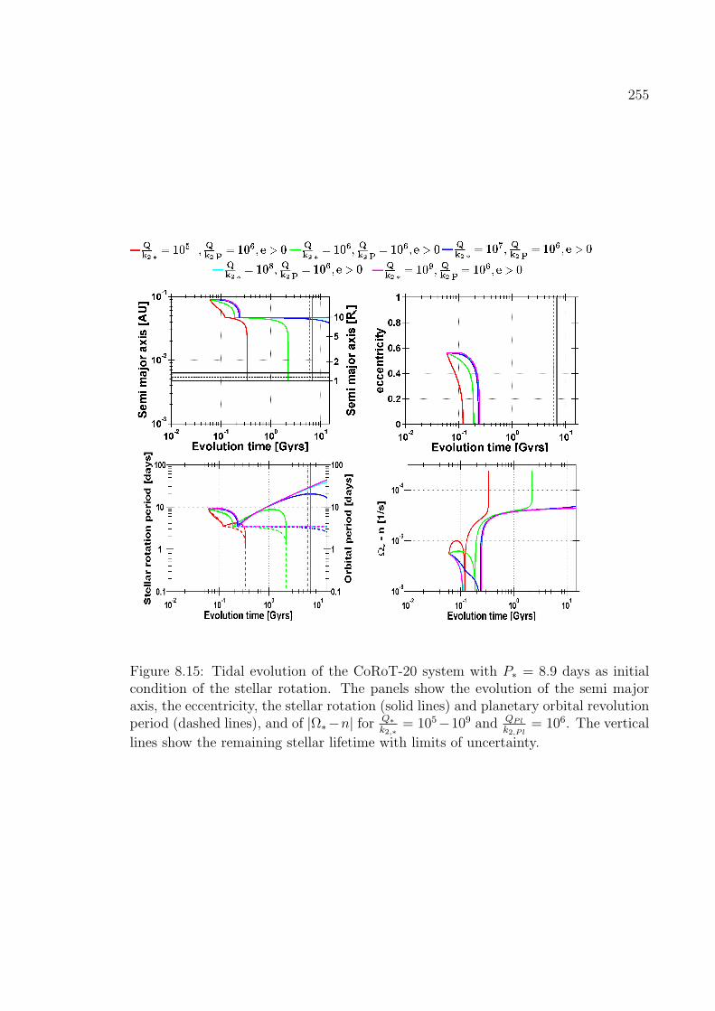
255
Figure 8.15: Tidal evolution of the CoRoT-20 system with P∗ = 8.9 days as initialcondition of the stellar rotation. The panels show the evolution of the semi majoraxis, the eccentricity, the stellar rotation (solid lines) and planetary orbital revolutionperiod (dashed lines), and of |Ω∗−n| for Q∗
k2,∗= 105−109 and QPl
k2,P l= 106. The vertical
lines show the remaining stellar lifetime with limits of uncertainty.

256
Apparently, the tidal evolution of the CoRoT-20 system changes only slightly for
different QPl
k2,P l= 104 − 106 if P∗ = 8.9 days is chosen as initial condition. Therefore,
this tidal evolution scenario will be discussed in detail for Q∗k2,∗
= 105 − 109 and the
average QPl
k2,P l= 105, only.
The system will evolve for every Q∗k2,∗
= 105 − 109 and QPl
k2,P linto a double syn-
chronous state within one hundred million years. This is in contrast to the evolution
of CoRoT-20 described in Sections 5.2 and 6.2. There, the system reached the double
synchronous state only for Q∗k2,∗
= 105 and QPl
k2,P l≥ 105.
This confirms one statement from Section 8.2: It is much easier to achieve a double
synchronous state Ω∗ = n from an initial condition Ω∗ > n (a supsynchronous orbit)
than from an initial condition Ω∗ < n (a subsynchronous orbit). As can be seen
on detailed inspection (Figure 8.16), tidal evolution is not even necessary to achieve
this state. If Q∗k2,∗
≥ 107, magnetic braking on its own moves the ’fictive’ double
synchronous state outwards towards the planetary orbit. Neither the semi major axis
nor the eccentricity changes during this brief initial phase.
Once a state Ω∗ = n is reached, apparently stellar and planetary tidal friction,
even for Q∗k2,∗
= 109 and QPl
k2,P l= 104 − 106, are sufficient to force the system into a
’true’ double synchronous state. The most telling sign for the double synchronous
orbit evolution is the efficient eccentricity dampening. As was described in Section 2.9,
a stable double synchronous orbit is not only characterized by Ω∗ = n. Furthermore,
the total and orbital angular momentum need to exceed Ltot,crit and Lorb,crit, which
is currently true for the CoRoT-20 system (Section 8.1). In addition, a true double
synchronous orbit can not be eccentric. Indeed, the evolution tracks here show that,
once the Ω∗ = n is reached, the eccentricity is damped very fast within the next one
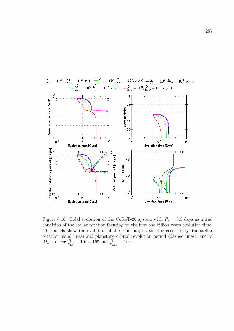
257
Figure 8.16: Tidal evolution of the CoRoT-20 system with P∗ = 8.9 days as initialcondition of the stellar rotation focusing on the first one billion years evolution time.The panels show the evolution of the semi major axis, the eccentricity, the stellarrotation (solid lines) and planetary orbital revolution period (dashed lines), and of|Ω∗ − n| for Q∗
k2,∗= 105 − 109 and QPl
k2,P l= 105.

258
hundred million years to zero for any Q∗k2,∗
= 105 − 109 and QPl
k2,P l. In contrast to that,
the non-synchronous evolution of the CoRoT-20 system shows that the eccentricity
may never reach zero within the remaining lifetime if Q∗k2,∗
≥ 108 and QPl
k2,P l(Sections 5.2
and 6.2). The fast eccentricity dampening in a true double synchronous configuration
shows that although Ω∗ = n is in principle a possible state for the CoRoT-20 system
within the limits of uncertainty, the large eccentricity of the orbit of CoRoT-20b
shows that the system cannot truly be in a double synchronous state.
Furthermore, once the eccentricity is damped to zero, magnetic braking imme-
diately decelerates the stellar rotation and stellar tidal friction on its own and is
not able to compensate by spinning-up the star at the current position. Apparently,
even with this favorable initial condition P∗(initial) = 8.9 days, the positive feed-
back effect between stellar and planetary tidal friction is needed to maintain a double
synchronous state despite magnetic braking. This result supports the reasoning ex-
plained in Section 8.2, which leads to the condition that an upper Q∗k2,∗ spinup
limit is
required to guarantee that tidal friction can maintain a stable double synchronous
orbit in the presence of magnetic braking.
Stellar tidal friction may, in principle, be able to spin up CoRoT-20 at a later
point in evolution if Q∗k2,∗
≤ 106 and the planet moves towards the star. At that
point, however, the system has lost so much angular momentum that the angular
momentum criteria for a double synchronous state are no longer fulfilled and a double
synchronous orbit is not possible. Instead, the planet will decay within the remaining
lifetime. Therefore, in terms of orbital stability due to stellar and planetary tidal
friction, the conclusions here are the same as in Section 5.2: Q∗k2,∗
= 107 − 108 is
required as a stability limit to guarantee that the planet does not reach the Roche

259
zone within the remaining lifetime. Double synchronicity can not save the system
from the decay because magnetic braking forces the system out of a possible double
synchronous state. A transient double synchronicity can force, however, the orbit to
become circular much earlier than under tidal evolution without reaching a double
synchronous state. See also Chapter F), which confirms this ’duality’ of the possible
evolution tracks of the CoRoT-20 system.
8.4.2 Limits on Q∗k2,∗
to currently maintain a double synchronousrotation state
As was previously shown by modeling the evolution of the CoRoT-3 and CoRoT-
15 system, these two systems may already be in a double synchronous state. This
depends on Q∗k2,∗
and magnetic braking .
It will now be assumed that these systems are currently in the process of being
forced into a double synchronous state by tidal friction. Based on this assumption,
the upper limit Q∗k2,∗
can be derived to achieve a double synchronous state despite
magnetic braking using equation (8.2.16) (Table 8.1).
This constraint is not applicable to systems currently not affected by magnetic
System Q∗k2,∗ upper limit ,rot
magnetic braking
CoRoT-3 4.5× 10⁶ K = 2.7× 1040 NmsCoRoT-3 4.5× 10⁷ K = 2.7× 1039 NmsCoRoT-15 4× 10⁷ K = 2.7× 1040 NmsCoRoT-15 4× 10⁸ K = 2.7× 1039 NmsCoRoT-20a 8.5× 10⁴ K = 2.7× 1040 Nms
a) applying aequiv = 0.063 AU to Eq. 8.2.16.
Table 8.1: Required Q∗k2,∗
for tidal friction to compensate magnetic braking at the
planet’s current position.

260
braking. Furthermore, it doesn’t necessarily require that the system evolves into a
double synchronous state within the remaining stellar lifetime. This yields Q∗k2,∗
≤
4.5× 10⁷ for CoRoT-3 and reduced magnetic braking and Q∗k2,∗
≤ 4× 10⁸ for CoRoT-
15 and reduced magnetic braking. After all, for CoRoT exoplanet host stars of
spectral type F, reduced magnetic braking appears to be a reasonable assumption
(Sections 6.1.2, and Chapter 7).
If it is further assumed that the orbits of CoRoT-3b and CoRoT-15b have evolved
into this approximately double synchronous state by tidal friction, another much
stronger constraint on Q∗k2,∗
can be put that does not depend on magnetic braking.
For this purpose, a minimal orbit variation in the past into the double synchronous
state is assumed. This approach is similar to the work done by Dermott (1979b) who
derived a constant onQJup
k2,Jupof Jupiter by requiring that the orbits of the Galilean
moons evolved into the Laplace resonances by tidal migration (See Section 2.8.1).
Using equation 2.6.21 and solving for Q∗k2,∗
yields the following upper limit that
needs to be fulfilled to allow for orbital migration:
Q∗
k2,∗=
392
(GM∗
)1/2R5
∗MPl
a13/20
[|1−
(aia0
)13/2|]∆t. (8.4.5)
Here, a0 is the current semi major axis and ai is the primordial semi major axis
from which the planet originated. The upper limit is derived by setting ai = a0±∆a,
where ∆a is set to 5% a0 and 10% a0, respectively, to allow for at least small variation
of the semi major axis in the past. The results are listed in Table 8.2. Q∗k2,∗
≤ 1× 10⁷
is required for CoRoT-3, and Q∗k2,∗
≤ 1 × 10⁸ is required for CoRoT-15 to allow for
tidal evolution.

261
System Q∗k2,∗ upper limit ,a
ai/a0
CoRoT-3 4± 1× 10⁷ 0.95CoRoT-3 3.1± 0.8× 10⁷ 1.05CoRoT-3 2.3± 0.7× 10⁷ 0.9CoRoT-3 1.4+0.3
−0.5 × 10⁷ 1.1CoRoT-15 4.2± 2.0× 10⁸ 0.95CoRoT-15 3.2± 1.6× 10⁸ 1.05CoRoT-15 2.4± 1.2× 10⁸ 0.9CoRoT-15 1.4+0.7
−4.4 × 10⁸ 1.1
Table 8.2: Required Q∗k2,∗
for tidal friction to allow for minimal migration in the past.
As can be seen, when comparing results from Tables 8.2 and 8.1, the same upper
limit of Q∗k2,∗
is derived from requiring stellar spin-up in the presence of reduced mag-
netic braking and from requiring orbital migration into a double synchronous state:
Q∗k2,∗
in the order of 107 for CoRoT-3 and Q∗k2,∗
in the order of 108 for CoRoT-15. When
excluding full magnetic braking for the stars CoRoT-3 and CoRoT-15 and favoring
Q∗k2,∗
≤ 107, the double synchronous orbit further remains stable in the remaining stel-
lar lifetime. The possible decay outlined in the previous section only takes place after
several billion years and takes much longer than the remaining lifetime.
It is interesting to note that to establish double synchronicity relatively small
Q∗k2,∗
≤ 107−108 are favored, whereas the orbital stability limit and tidal spin up limit
from Sections 5 and 6 require Q∗k2,∗
≥ 107 − 108.
As was shown in Section 3.1, when a system approaches a double synchronous
state, i.e., if the tidal frequency ω = 2|Ω∗ − n| → 0, it is expected that Q∗ → ∞.
Instead, the exact opposite is seen. This may be explained by suggesting that the
weak friction case is no longer valid. Instead, dynamical tides are at work because,
on its way to synchronicity, the tidal frequency has a higher chance to meet stellar

262
eigenfrequencies. Dynamical tides dissipate tidal energy more efficiently (Zahn, 1977),
reducing Q∗. Therefore, dynamical tides can easily and consistently explain why Q∗k2,∗
apparently becomes smaller instead of larger when ω → 0.

Chapter 9
Summary and Discussion
The investigation of tidal friction due to tides raised on the star by the planet (stellar
tidal friction) and due to tides raised by the star on the planet (planetary tidal fric-
tion), may be used to constrain Q∗k2,∗
for main sequence stars and different scenarios.
In this work, CoRoT planetary systems with close-in Jupiter-mass planets around
slowly rotating and fast rotating stars, short-period Jupiter-mass exoplanets on cir-
cular and eccentric orbits, short-period brown dwarfs near double synchronous states
and a low-mass Super-Earth planet were investigated.
It was found that the majority of the CoRoT planets may migrate towards the
star (because Ω∗ < n) and be destroyed within the Roche zone if Q∗k2,∗
≤ 106. For
Q∗k2,∗
= 105, many planets - including the Super-Earth CoRoT-7b - would reach the
Roche zone even within one hundred million years, which is only circa 1% of the total
lifetime of a main sequence star. The planets would be destroyed ’in the blink of an
eye’ on astronomical time scales, making it statistically improbable to find them.
In contrast to that, such planetary systems are ubiquitous and frequently found,
as the distribution of the so far discovered exoplanets’ semi major axes shows (Sec-
tion 1.5). Furthermore, the fact that such systems are frequently discovered by transit
263

264
surveys, like the CoRoT space mission, proves that such close-in massive planets are
not rare. After all, transiting planets represent only≈ 5−10% of all planetary systems
due to the strong observation bias regarding the orbital plane, limiting the detection
to planetary systems whose orbital plane is parallel to the line-of-sight (Section 1.3.2).
The detection of Kepler-10b, the second transiting terrestrial planet after CoRoT-
7b, shows that even short-period Super-Earths are probably not rare objects and
should survive over timescales of billion years. Kepler-10b (Batalha et al., 2011) and
CoRoT-7b (Table A.1) are very similar in planetary parameters, except for the age:
Kepler-10b is a ten billion years older version of CoRoT-7b. This suggests that such
planets should survive over the timescales of several billion years.
With this reasoning, Q∗k2,∗ stable
= 107 − 108 can be derived as the com-
mon lower orbital stability limit. Indeed, this result is consistent with the Q∗k2,∗
constraint derived by Patzold and Rauer (2002) ( Q∗k2,∗
≥ 108), Rasio et al. (1996)
( Q∗k2,∗
= 4× 10⁸), and Carone and Patzold (2007) ( Q∗k2,∗
≥ 3× 10⁷), but contradicts the
Q∗k2,∗
- values favored by Jackson et al. (2008) ( Q∗k2,∗
= 105.5), Dobbs-Dixon et al. (2004)
( Q∗k2,∗
= 105 − 106), and Lin et al. (1996)( Q∗k2,∗
= 105).
Another, independent argument against Q∗k2,∗
≤ 106 and in favor of Q∗k2,∗
≥ 107−108
can be derived from the stellar rotation evolution. If a planet migrates towards the
Roche zone, conservation of angular momentum leads to efficient stellar spin-up com-
pensating even strong magnetic braking in low-mass main sequence stars. The stellar
rotation period versus age distribution of the CoRoT planet host stars (Figures 6.8
and 6.9) shows the expected behavior for stars whose rotation is decelerated by mag-
netic braking with increasing age, except for CoRoT-17. Therefore, a tidal spin-up
constraint for Q∗k2,∗
is derived by requiring tidal friction to be weaker than

265
magnetic braking at the current position, which yields Q∗k2,∗ spin−up
> 106, and
agrees nicely with the orbital stability limit.
CoRoT-17, on the other hand, is the one star that seems to be rotating faster than
its age suggests (Figure 6.8, P∗ = 18 ± 2 days at an age of 10.7 billion years). The
star does not show, however, the fast tidal spin-up expected for stars whose planets
enter the Roche zone. This would require rotation periods in the order of 1− 10 days
(Section 6). The star appears rather to be moderately spun-up at the end of its
lifetime. It was shown in Section 6 that old stars are susceptible to being spun up by
comparatively large Q∗k2,∗
= 107. Indeed, the tidal Q∗k2,∗ spin−up
limit at the position
of CoRoT-17b requires Q∗k2,∗
≈ 4 × 10⁷ to account for the current moderate
spin-up despite magnetic braking. This still agrees with the previously derived
orbital stability and stellar spin up limit on Q∗k2,∗
by excluding Q∗k2,∗
= 105 − 106. But
to allow for tidal spin-up, Q∗k2,∗
has to be smaller than 109 for CoRoT-17.
Otherwise no tidal evolution would occur.
Q∗k2,∗
≈ 107 would allow for long-term stability of short-period Jupiter mass planets,
allow for moderate tidal spin-up of old stars, but would not allow for long-term
stability of short-period brown dwarfs as can be seen by inspecting Eq. 5.1.2. This
stability threshold is proportional to MPl. If Jupiter mass planets require Q∗k2,∗
≥ 107
for long-term stability, brown dwarfs with masses MPl ≥ 10MJup require Q∗k2,∗
≥ 108
on similar orbits. Indeed, in Section 1.5 an erosional feature may be present, which
warrants additional investigation. This is, however, not within the scope of this work.
The possible erosion of short-period brown dwarfs and Jupiter mass planets and
the corresponding possible tidal spin-up of stars should be taken into account before

266
trying to derive the age of a star by Gyrochronology. Otherwise, this age determina-
tion method may yield an age too small. Old stars towards the end of their lifetime,
like CoRoT-17, are particularly susceptible for tidal spin-up. Even stars that don’t
currently have a close-in companion may have been tidally spun-up in the past when
the corresponding companion has migrated towards the Roche zone and has been
destroyed there. Interestingly, abnormally fast rotating stars are not unknown. So-
called ’blue stragglers’ are reported, for example, by Fuhrmann et al. (2011) who
identified a F6V star whose rotation is spun-up through interaction with an unseen
0.42MSun companion.
Another interesting scenario in terms of tidal interactions are presented by CoRoT
planets on eccentric orbits. It was shown that for moderate to small orbital eccentric-
ity e ≤ 0.3, represented by CoRoT-16b, planetary tidal friction with QPl
k2,P l= 104− 106
(taken from the gas giants in our Solar System), acts on much shorter timescales
than stellar tidal friction. Planetary tidal friction, in this case, leads to eccentric-
ity dampening within one billion years conserving the orbital angular momentum.
Therefore, the secular stability of short-period planets with e ≤ 0.3 can be
evaluated with the same equations derived for circular orbits but using
aequiv = a(1 − e2), assuming QPl
k2,P l≤ 106. The efficient eccentricity dampening by
planetary tidal friction explains the fact that most close-in extrasolar planets have
circular orbits. That the orbit of CoRoT-16b, with an age of about six billion years,
is still quite eccentric suggests that the orbit was even more eccentric in the past.
This warrants additional investigation that is, however, not within the scope of this
work.
267
It was found that aequiv can not be used for planets like CoRoT-10b and CoRoT-
20b. For e ≥ 0.5, planetary and stellar tidal friction may act on the same
time scales, if Q∗k2,∗
= 105 − 106 and QPl
k2,P l= 104 − 106. This would lead to
a positive feedback effect, decreasing the semi major axis/spinning up
the star much stronger than stellar and planetary tidal friction would on
their own. This feedback effect may even destabilize planets that would
otherwise be stable under tidal friction or may force systems into double
synchronous rotation that can not be maintained by stellar tidal friction
alone. To avoid such effects, Q∗k2,∗
has to be again larger than 106.
Another interesting tidal interaction scenario is presented by the CoRoT-11 sys-
tem: A short-period Jupiter-mass planet around a fast-spinning F-star. Here, the
tidal evolution depends not only on Q∗k2,∗
but also on magnetic braking efficiency.
• Scenario 1: The star is braked down efficiently by magnetic braking similar in
strength than for lower mass stars M∗ < 1.1MSun.
Regardless of the strength of stellar tidal friction, the planetary system CoRoT-
11 will become within a few hundred million years a ’normal’ planetary system
with a close-in exoplanet around a slowly rotating star. In this case, the orbital
stability limit Q∗k2,∗
= 107 − 108 is again required to keep the planet CoRoT-11b
from reaching the Roche zone within the remaining lifetime.
• Scenario 2: The star is braked down by reduced magnetic braking that is ten
times less efficient than in scenario 1.
The rotation of CoRoT-11 is still braked down relatively fast within one billion
years, until a state is reached where again Ω∗ < n and the planet may migrate
towards the star again. The planet will not reach the Roche zone within the
268
remaining lifetime if Q∗k2,∗
≥ 107. Interestingly, the same may be true for Q∗k2,∗
=
105 due to a fast initial outward migration phase.
• Scenario 3: The star is not slowed down by magnetic braking.
CoRoT-11b may migrate away from the star, if Q∗k2,∗
≤ 107. The stellar rotation
period of CoRoT-11 is tidally spun-down by less than one day even if Q∗k2,∗
= 105
which is negligible.
Only in the absence of magnetic braking can stars like CoRoT-11 maintain their
fast rotation over secular timescales. CoRoT-11 itself, however, is relatively young
(age=2 ± 1 billion years). The distribution of stellar rotation period versus age for
CoRoT stars of spectral type F(Figure 6.9) seems to indicate a reduced magnetic
braking mechanism. If spectral type F-stars are indeed subjected to at least
moderate magnetic braking, then the following predication can be made:
Only young stars can rotate faster than their close-in Jupiter mass planet
revolves around it, because magnetic will decelerate the star within one
billion years. Therefore, the fast stellar rotation is only a transient state.
In the long run, such systems still require Q∗k2,∗ stable
≥ 107 for long-term
stability.
Finally, several possible double synchronous states were identified in the CoRoT
subsample and their evolution was investigated:
• Of all investigated CoRoT planetary systems CoRoT-3, CoRoT-6, CoRoT-9,
CoRoT-10, CoRoT-15, and CoRoT-20 currently satisfy the angular momenta
conditions to achieve a double synchronous state Ω∗−n described by Hut (1980).
• The CoRoT-4 system is a ’false’ double synchronous state because it does not

269
satisfy the angular momentum criteria by Hut (1980).
• CoRoT-9b and CoRoT-6b are currently too far away from their stars, however,
to establish synchronization within the remaining stellar lifetime.
• Due to the large orbital eccentricity, the CoRoT-20 system can not currently
be in double synchronous rotation; even though the limits of uncertainties for
the stellar rotation allow in principle Ω∗ = n.
• CoRoT-20 may, however, reach a double synchronous state due the positive
feedback effect between planetary and tidal friction because the orbital eccen-
tricity is very large. If this happens, then the eccentricity is damped to zero
within a few hundred million years. When the eccentricity has become zero and
planetary tidal friction seizes to act on the system, stellar tidal friction on its
own will not be able to compensate magnetic braking for any Q∗k2,∗
= 105 − 109
and the double synchronous orbit can not be maintained.
• In addition, magnetic braking will remove so much angular momentum from
the CoRoT-20 system within the next one billion years, that the system will
no longer meet all the angular momenta requirements to establish a double
synchronous state (Hut, 1981).
• CoRoT-3 and CoRoT-15 may be systems that are evolving into ’true’ double
synchronous states.
• In the presence of magnetic braking, a double synchronous orbit will decay.
In other words, the planet may still migrate towards the star and the stellar
rotation will be ’dragged’ along.

270
• A mathematical formulation was derived that describes that decay. Once tidal
friction has forced the system into corotation, the subsequent decay of the dou-
ble synchronous orbit does not depend on Q∗k2,∗
but on the efficiency of magnetic
braking.
• If CoRoT-3 and CoRoT-15 experience efficient magnetic braking like spectral
type G-stars, the double synchronous orbit will decay and the brown dwarfs
may even reach the Roche limit within the remaining lifetime.
• If CoRoT-3 and CoRoT-15 experience reduced magnetic braking or no magnetic
braking at all, the double synchronous states are stable within the remaining
lifetime.
This leads to the following prediction: Only F-stars are capable to maintain
a double synchronous state over secular timescales with a close-in massive
planetary companion. In addition, it was found that in order to maintain
a double synchronous state despite magnetic braking, the following con-
straints can be derived for Q∗k2,∗
: Q∗k2,∗
≤ 107 for CoRoT-3, and Q∗k2,∗
≤ 108 for
CoRoT-15. If it is further required that CoRoT-3b and CoRoT-15b mi-
grated towards the double synchronous orbit, again, Q∗k2,∗
≤ 107 for CoRoT-3,
and Q∗k2,∗
≤ 108 for CoRoT-15 is derived when allowing for a 10% change in
the semi major axis.
The Q∗k2,∗
-values required to force the CoRoT-3 and CoRoT-15 system into a double
synchronous state ( Q∗k2,∗
≤ 107 − 108) barely overlap with the Q∗k2,∗
-values required for
orbital stability in non-synchronous systems ( Q∗k2,∗
≥ 107 − 108).
For double synchronous systems, the tidal frequency ω = |2Ω∗ − n| ≈ 0 is orders

271
of magnitude smaller than the tidal frequency in non-synchronous systems where
ω = 2|Ω∗ − n| ≈ 2n which is in the order of 10−3 − 10−5 1/s.
In the weak friction assumption that is used in this work, Q∗ is related to the tidal
frequency by
Q∗ =|ω2
0 − ω2|ω/τd
, (9.0.1)
where the resonance frequency ω0 and the damping timescale τd are constants. There-
fore, Q∗k2,∗
is expected to grow as ω → 0. This is, however, not the result that is derived
here. Q∗k2,∗
for double synchronous states (ω → 0) equals or is even smaller than the
values derived for the non-synchronous states.
This contradiction can be solved by suggesting that dynamical tides are at work in
double synchronous cases because the tidal frequency meets stellar eigenfrequencies
as 2|Ω∗ − n| → 0. This leads in turn to an increase in tidal energy dissipation
and to a reduction of Q∗. The work by Penev and Sasselov (2011) supports this
conclusion: ’the time variable tidal perturbation can resonantly excite inertial waves
in the star, thus resulting in several orders of magnitude larger shear, and hence
dissipation, compared to the static tide’.
Indeed, this explanation also solves the deviation between the low Q∗k2,∗
= 105−106
favored by several authors (Jackson et al., 2009; Lin et al., 1996; Dobbs-Dixon et al.,
2004) from synchronization time scales of double synchronous binary stars (Meibom
and Mathieu, 2005), and the relatively high Q∗k2,∗
≥ 107 − 108 required for orbital
stability as found in this work and supported by Rasio et al. (1996); Patzold and
Rauer (2002); Carone and Patzold (2007).
As the results in this work and the work of Penev and Sasselov (2011) confirm,
it is probably not a good idea to apply tidal dissipation factors derived from double

272
synchronous states to tidal friction cases with Ω∗ ≪ n. This is a completely differ-
ent tidal frequency regime with possibly very different tidal dissipation efficiencies.
Therefore, one has to take care when applying tidal friction and tidal dissipation
models. There are a lot of underlying assumptions that have to be investigated prior
to applying them to cases, for which they were not developed. Otherwise the results
may be misleading.

Appendix
273

Appendix A
CoRoT planet references
274

275
Table A.1: References for the parameters of the CoRoT planetary systems.
System ReferencesCoRoT-1 Barge et al. (2008)CoRoT-2 Bouchy et al. (2008), Alonso et al. (2008)CoRoT-3 Deleuil et al. (2008)CoRoT-4 Moutou et al. (2008)CoRoT-5 Rauer et al. (2009)CoRoT-6 Fridlund et al. (2010)CoRoT-7 Leger et al. (2009), Queloz et al. (2009), Bruntt et al.
(2010), Hatzes et al. (2010), Hatzes et al. (2011)CoRoT-8 Borde et al. (2010)CoRoT-9 Deeg et al. (2010)CoRoT-10 Bonomo et al. (2010)CoRoT-11 Gandolfi et al. (2010)CoRoT-12 Gillon et al. (2010)CoRoT-13 Cabrera et al. (2010)CoRoT-14 Tingley et al. (2011)CoRoT-15 Bouchy et al. (2011)CoRoT-16 In PreparationCoRoT-17 Csizmadia et al. (2011)CoRoT-18 Hebrard et al. (2011)CoRoT-19 Guenther et al. (2012)CoRoT-20 Deleuil et al. (2011)CoRoT-21 Patzold and the CoRoT-Team, in preparation

Appendix B
Tidal evolution of CoRoT-4 andCoRoT-9
276

277
Figure B.1: Tidal evolution of the of the CoRoT-4 system for for Q∗k2,∗
= 105 − 109,QPl
k2,P l= 105, and full, reduced and without magnetic braking. The vertical lines show
the remaining stellar lifetime with limits of uncertainty.
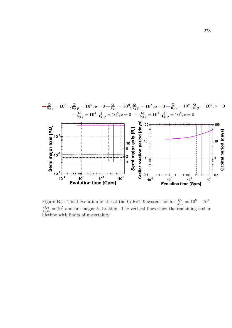
278
Figure B.2: Tidal evolution of the of the CoRoT-9 system for for Q∗k2,∗
= 105 − 109,QPl
k2,P l= 105 and full magnetic braking. The vertical lines show the remaining stellar
lifetime with limits of uncertainty.

Appendix C
|Ω∗ − n| evolution for close-inCoRoT-planets
279

280
Figure C.1: The evolution of |Ω∗ − n| for the planetary systems CoRoT-1,-2,-7,-8,-12,-13,-17,-18 for the next 1.5× 10¹⁰ years, Q∗
k2,∗= 105 − 109.

281
Figure C.2: The evolution of |Ω∗−n| for the planetary systems CoRoT-5,-14,-19 andfull magnetic braking for the next 1.5× 10¹⁰ years, Q∗
k2,∗= 105 − 109.

282
Figure C.3: The evolution of |Ω∗−n| for the planetary systems CoRoT-5,-14,-19 andreduced magnetic braking for the next 1.5× 10¹⁰ years, Q∗
k2,∗= 105 − 109.

283
Figure C.4: The evolution of |Ω∗−n| for the planetary systems CoRoT-5,-14,-19 andwithout magnetic braking for the next 1.5× 10¹⁰ years, Q∗
k2,∗= 105 − 109.

284
Figure C.5: The evolution of |Ω∗−n| for the planetary systems CoRoT-10,-16,-20 forthe next 1.5× 10¹⁰ years, Q∗
k2,∗= 105 − 109 and QP
k2,P= 104.

285
Figure C.6: The evolution of |Ω∗−n| for the planetary systems CoRoT-10,-16,-20 forthe next 1.5× 10¹⁰ years, Q∗
k2,∗= 105 − 109 and QP
k2,P= 105.

286
Figure C.7: The evolution of |Ω∗−n| for the planetary systems CoRoT-10,-16,-20 forthe next 1.5× 10¹⁰ years, Q∗
k2,∗= 105 − 109 and QP
k2,P= 106.

287
Figure C.8: The evolution of |Ω∗−n| for the planetary systems CoRoT-6, and CoRoT-11 for the next 1.5× 10¹⁰ years, Q∗
k2,∗= 105 − 109.

288
Figure C.9: The evolution of |Ω∗−n| for the planetary systems CoRoT-3, and CoRoT-15 for the next 1.5× 10¹⁰ years, Q∗
k2,∗= 105 − 109.

Appendix D
Evolution of the rotation of CoRoTplanets on eccentric orbits
Figures D.1, D.2, and D.3 show the tidal evolution of the planet’s rotation period
starting with PPl(initial) = 2.5 days1. The planetary rotation of CoRoT-10b, -16b,
and -20b is quickly forced into a synchronized state. This happens before the orbit
becomes circular. Therefore, the planetary rotation rate ΩPl is not synchronized with
the mean orbital revolution rate n but rather pseudo-synchronized with (Hut, 1981)
npseudo = n
(1 + 6e2 +
3
8e4 +
223
8e6). (D.0.1)
Therefore, the tidal planetary frequency 2|ΩPl − n| evolves with
2|ΩPl − n| = 2n
(6e2 +
3
8e4 +
223
8e6), (D.0.2)
starting for the planets CoRoT-10b,-16b, and 20b with
Planet 2|ΩPl − n|start
CoRoT-10b 4.66n
CoRoT-16b 1.12n
CoRoT-20b 5.6n
1This value was chosen as a medium value between the fast rotation of 10 hours and 10 daysselected in Section 3.2.
289

290
and approaching zero, as the eccentricity is damped to zero as well.
The planetary rotation of CoRoT-9b on the other hand may, depending on QPl
k2,P l,
never become synchronized or take several hundred million years to several billion
years to evolve into a pseudo-synchronized state.
Figure D.1: The tidal evolution of the rotation period of the planets CoRoT-9b,-10b,-16b, and CoRoT-20b for the next 1.5 × 10¹⁰ years, for Q∗
k2,∗= 105.5, 106, 107, 108, 109
(solid lines) and QPl
k2,P l= 104. The vertical lines show the remaining lifetime of the
system. The dashed-dotted lines show the evolution of the mean orbital revolutionperiod for comparison. npseudo is depicted by a dotted line which is for CoRoT-10b,-16b, 20b hidden by the planetary rotation evolution because – apart from a verybrief initial phase – ΩPl = npseudo.

291
Figure D.2: The tidal evolution of the rotation period of the planets CoRoT-9b,-10b,-16b, and CoRoT-20b for the next 1.5 × 10¹⁰ years, for Q∗
k2,∗= 105.5, 106, 107, 108, 109
(solid lines) and QPl
k2,P l= 105. The vertical lines show the remaining lifetime of the
system. The dashed-dotted lines show the evolution of the mean orbital revolutionperiod for comparison. npseudo is depicted by a dotted line which is for CoRoT-10b,-16b, 20b hidden by the planetary rotation evolution because – apart from a verybrief initial phase – ΩPl = npseudo

292
Figure D.3: The tidal evolution of the rotation period of the planets CoRoT-9b,-10b,-16b, and CoRoT-20b for the next 1.5 × 10¹⁰ years, for Q∗
k2,∗= 105.5, 106, 107, 108, 109
(solid lines) and QPl
k2,P l= 106. The vertical lines show the remaining lifetime of the
system. The dashed-dotted lines show the evolution of the mean orbital revolutionperiod for comparison. npseudo is depicted by a dotted line which is for CoRoT-10b,-16b, 20b hidden by the planetary rotation evolution because – apart from a verybrief initial phase – ΩPl = npseudo

Appendix E
Integration method
There exists a number of numerical integrators (Vallado (2001), and Gould et al.
(2006)) suitable to solve ordinary differential equations. In this work, the RK4(5)
algorithm is used, a special case of the classical Runge-Kutta method (Gould et al.,
2006).
The Runga-Kutta method was first formulated in 1895 by Carl Runge and later
improved by Heun and Kutta. To explain this method, the following first-order
differential equation is considered:
f(x, t) =dx
dt, (E.0.1)
where f(x, t) is the rate of the solution at position x and time t. Let xn(tn) be the
initial condition. To obtain the solution xn+1(tn+1), the rate is evaluated s times in the
time interval [tn, tn+1]. Each evaluation yields a slightly different rate ki = f(xi, ti).
The solution is derived by using a weighted mean of the intermediate rates for the
time step h = tn+1 − tn.
The Runga-Kutta algorithm with number of intermediate steps s is described by:
xn+1(tn+1) = xn(tn) + h
s∑i=1
biki, (E.0.2)
293

294
where the rates ki are developed iteratively:
k1 = f(xn, tn)
k2 = f(xn + k1a21h, tn + c2h)
k3 = f(xn + k1a31h+ k2a32h, tn + c3h)
...
ks = f(xn + k1as1h+ k2as2h+ · · ·+ ks−1as,s−1h, tn + csh)
The coefficients bi, ci with i = 1, 2, . . . s and aij with 1 ≤ j < i ≤ s can be derived
from the coefficient tableau of the selected Runge-Kutta algorithm:
c1 0 0 0 0
c2 a21 0 0 0...
.... . . 0 0
cs as1 · · · as,s−1 0
b1 b2 · · · bs
The coefficients are determined such that
s∑i=1
bi = 1 ci =i−1∑j=1
aij and c1 = 0. (E.0.3)
The accuracy of the numerical integration depends on the step size h. This can
be estimated, for example, by applying the method with step size h and h/2, and by
comparing the solutions with each other. The RK4(5) algorithm uses another method
to derive the accuracy at each time step. It simultaneously runs a fourth and fifth
order Runge-Kutta method. The difference between the two solutions is the accuracy
of the 4th order solution1. RK4(5) is an adaptive time step algorithm. The user se-
lects beforehand the relative accuracy required for the integration and the algorithm
reduces or increases the step size until the accuracy criterium is met. In this work,
the relative accuracy is set to 10−8. The coefficient tableau of the RK4(5) algorithm is:
1A Runga-Kutta method is of order p if it has the local truncation error O(hp+1).

295
0 0 0 0 0 0 0 0
15
15
0 0 0 0 0 0
310
340
940
0 0 0 0 0
45
4445
−5615
329
0 0 0 0
89
193726561
−253602187
644486561
−212729
0 0 0
1 90173168
−35533
467325247
49176
− 510318656
0 0
1 35384
0 5001113
125192
−21876784
1184
0
35384
0 5001113
125192
−21876784
1184
0
517957600
0 757116695
393640
− 92097339200
1872100
140
The validity of the results derived with the RK4(5) algorithm can be tested by
computing the tidal evolution of a planetary system without magnetic braking. If
the numerical integration is implemented with acceptable accuracy, then the total
angular momentum should remain constant during the whole computation2.
This will be shown for one example: The tidal evolution of the CoRoT-21b system
for Q∗k2,∗
= 105 and without magnetic braking is computed. This system is selected
because the rate of change a is one of the largest: The planet will reach the Roche
limit in 7.6 million years for Q∗k2,∗
= 105 (Section 5.1.2, Figure 5.2). Figure E.1 shows
the total angular momentum Ltot, the orbital angular momentum Lorb, the stellar
rotational angular momentum Lrot,∗, and the planetary angular momentum Lrot,P l
for this evolution track.
Ltot appears to be constant over the evolution time. Furthermore, the total angular
momentum is Ltot(t0) = 7.0894 × 1042Nms at the start time t0 = 60 million years.
At the end time tend = 67 million years, the total angular momentum is Ltot(tend) =
7.0900× 1042Nms. This corresponds to a relative change of 0.0085%.
As a control, the tidal evolution of the CoRoT-21b system for Q∗k2,∗
= 109 and
without magnetic braking is computed and the angular momenta are compared (Fig-
ure E.2). Ltot appears to be constant over the evolution time. Furthermore, the total
angular momentum is Ltot(t0) = 7.0894 × 1042Nms at the start time t0 = 60 mil-
lion years. At tend = 15 billion years, the total angular momentum is Ltot(tend) =
7.0884× 1042Nms. This corresponds to a relative change of 0.0141%.
These results support the conclusion that the RK4(5) algorithm yields indeed
2Magnetic braking has to be switched off for this accuracy test, because otherwise the stellarwind would remove angular momentum from the planetary system.

296
Figure E.1: The evolution of the total angular momentum Ltot, the orbital angularmomentum Lorb, the stellar rotational angular momentum Lrot,∗, and the planetaryangular momentum Lrot,P l during the tidal evolution of the CoRoT-21 system forQ∗k2,∗
= 105. The rotation of the planet was initialized with a rotation period Prot,P l =
10 hours which is rapidly synchronized with the revolution period Porb = 2.72 days.
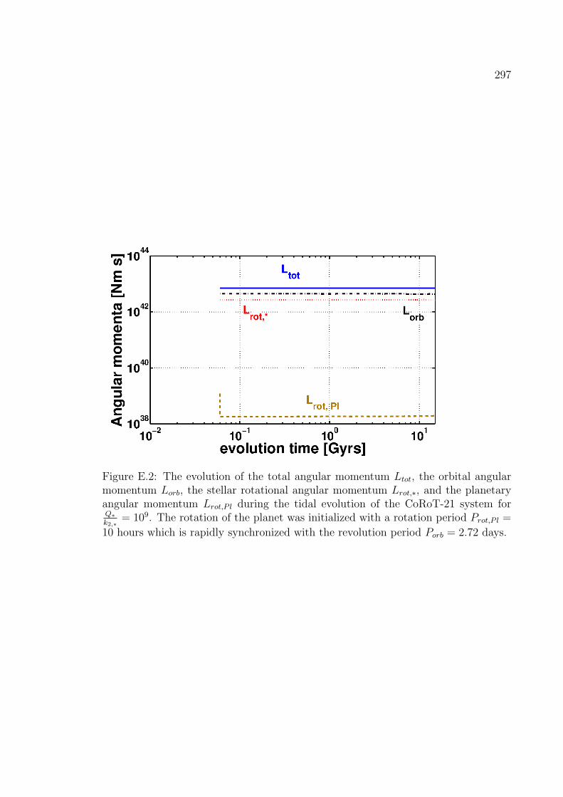
297
Figure E.2: The evolution of the total angular momentum Ltot, the orbital angularmomentum Lorb, the stellar rotational angular momentum Lrot,∗, and the planetaryangular momentum Lrot,P l during the tidal evolution of the CoRoT-21 system forQ∗k2,∗
= 109. The rotation of the planet was initialized with a rotation period Prot,P l =
10 hours which is rapidly synchronized with the revolution period Porb = 2.72 days.

298
sufficiently accurate results.

Appendix F
Model sensitivity analysis
In this work, the models did not take the uncertainties of the input parameters into
account. This will now be investigated in this chapter. A representative planetary
system is selected for each subcase discussed in this work and the model input pa-
rameters are varied using a Monte-Carlo method. The models investigated in this
work start with the following initial conditions:
a±∆a
P∗ ±∆P∗
e±∆e
PPl ± PPl (F.0.1)
It was shown that the energy and angular momentum of the planetary rotation is
negligible compared to the stellar rotation and planetary orbit (Section 3.3), therefore
it can be assumed that the tidal evolution does not depend on PPl.
To investigate the model sensitivity for the initial conditions a, P∗, and e – the
latter is only important for planets on eccentric orbits–, a set of one hundred start
parameters are randomly chosen within limits of uncertainty. The tidal evolution is
computed for each start condition of this set.
299
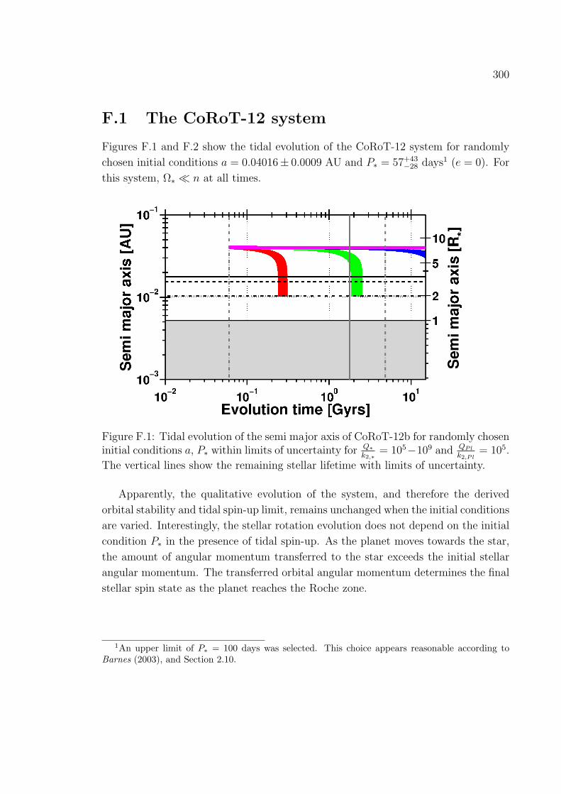
300
F.1 The CoRoT-12 system
Figures F.1 and F.2 show the tidal evolution of the CoRoT-12 system for randomly
chosen initial conditions a = 0.04016± 0.0009 AU and P∗ = 57+43−28 days
1 (e = 0). For
this system, Ω∗ ≪ n at all times.
Figure F.1: Tidal evolution of the semi major axis of CoRoT-12b for randomly choseninitial conditions a, P∗ within limits of uncertainty for Q∗
k2,∗= 105−109 and QPl
k2,P l= 105.
The vertical lines show the remaining stellar lifetime with limits of uncertainty.
Apparently, the qualitative evolution of the system, and therefore the derived
orbital stability and tidal spin-up limit, remains unchanged when the initial conditions
are varied. Interestingly, the stellar rotation evolution does not depend on the initial
condition P∗ in the presence of tidal spin-up. As the planet moves towards the star,
the amount of angular momentum transferred to the star exceeds the initial stellar
angular momentum. The transferred orbital angular momentum determines the final
stellar spin state as the planet reaches the Roche zone.
1An upper limit of P∗ = 100 days was selected. This choice appears reasonable according toBarnes (2003), and Section 2.10.

301
Figure F.2: Tidal evolution of the stellar rotation of CoRoT-12 for randomly choseninitial conditions a and P∗ within limits of uncertainty for Q∗
k2,∗= 105 − 109 and
QPl
k2,P l= 105. The vertical lines show the remaining stellar lifetime with limits of
uncertainty.
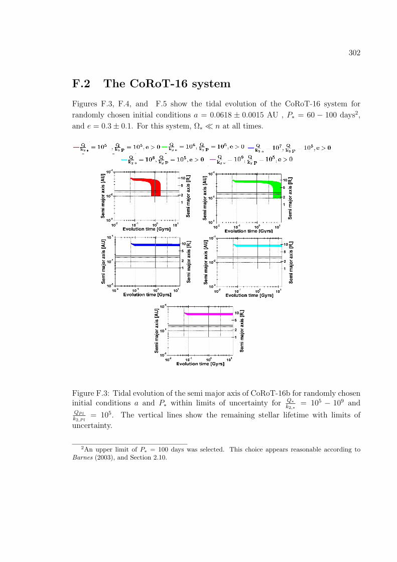
302
F.2 The CoRoT-16 system
Figures F.3, F.4, and F.5 show the tidal evolution of the CoRoT-16 system for
randomly chosen initial conditions a = 0.0618 ± 0.0015 AU , P∗ = 60 − 100 days2,
and e = 0.3± 0.1. For this system, Ω∗ ≪ n at all times.
Figure F.3: Tidal evolution of the semi major axis of CoRoT-16b for randomly choseninitial conditions a and P∗ within limits of uncertainty for Q∗
k2,∗= 105 − 109 and
QPl
k2,P l= 105. The vertical lines show the remaining stellar lifetime with limits of
uncertainty.
2An upper limit of P∗ = 100 days was selected. This choice appears reasonable according toBarnes (2003), and Section 2.10.

303
Figure F.4: Tidal evolution of the stellar rotation of CoRoT-16 for randomly choseninitial conditions a and P∗ within limits of uncertainty for Q∗
k2,∗= 105 − 109 and
QPl
k2,P l= 105. The vertical lines show the remaining stellar lifetime with limits of
uncertainty.

304
Figure F.5: Tidal evolution of the orbital eccentricity of CoRoT-16b for randomlychosen initial conditions a and P∗ within limits of uncertainty for Q∗
k2,∗= 105−109 and
QPl
k2,P l= 105. The eccentricity evolution does not depend on Q∗
k2,∗. The vertical lines
show the remaining stellar lifetime with limits of uncertainty.
Evidently, the tidal evolution of the semi major axis of CoRoT-16b and the stellar
rotation period of CoRoT-16 system varies more strongly with initial conditions forQ∗k2,∗
≤ 106 than the tidal evolution of the semi major axis of CoRoT-12b and the
stellar rotation of CoRoT-12. The eccentricity evolution, on the other hand, does not
very strongly with initial conditions. The strong variation of the a and P∗-evolution
is not surprising because for the evaluation of the CoRoT-16-system an additional
parameter, the orbital eccentricity, is introduced. The tidal model of the CoRoT-16
system is sensitive to three input parameters and not to two input parameters like
the tidal model of the CoRoT-12 system. Still, the qualitative results with respect toQ∗k2,∗
remain valid for this system as well because the tidal models yield qualitatively
similar results and depend more strongly on Q∗k2,∗
than on the initial conditions.
F.3 The CoRoT-20 system
Figures F.6, F.7, and F.8 show the tidal evolution of the CoRoT-20 system for
randomly chosen initial conditions a = 0.0618 ± 0.0015 AU , P∗ = 11.5 ± 2.6 days,
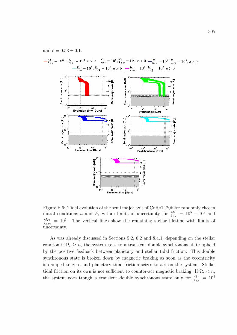
305
and e = 0.53± 0.1.
Figure F.6: Tidal evolution of the semi major axis of CoRoT-20b for randomly choseninitial conditions a and P∗ within limits of uncertainty for Q∗
k2,∗= 105 − 109 and
QPl
k2,P l= 105. The vertical lines show the remaining stellar lifetime with limits of
uncertainty.
As was already discussed in Sections 5.2, 6.2 and 8.4.1, depending on the stellar
rotation if Ω∗ ≥ n, the system goes to a transient double synchronous state upheld
by the positive feedback between planetary and stellar tidal friction. This double
synchronous state is broken down by magnetic braking as soon as the eccentricity
is damped to zero and planetary tidal friction seizes to act on the system. Stellar
tidal friction on its own is not sufficient to counter-act magnetic braking. If Ω∗ < n,
the system goes trough a transient double synchronous state only for Q∗k2,∗
= 105

306
Figure F.7: Tidal evolution of the stellar rotation of CoRoT-20 for randomly choseninitial conditions a and P∗ within limits of uncertainty for Q∗
k2,∗= 105 − 109 and
QPl
k2,P l= 105. The vertical lines show the remaining stellar lifetime with limits of
uncertainty.

307
Figure F.8: Tidal evolution of the orbital eccentricity of CoRoT-20b for randomlychosen initial conditions a and P∗ within limits of uncertainty for Q∗
k2,∗= 105 − 109
and QPl
k2,P l= 105. The vertical lines show the remaining stellar lifetime with limits of
uncertainty.
308
and QPl
k2,P l= 105 − 106. In any case, the planet will reach the Roche limit within
the remaining lifetime if Q∗k2,∗
≤ 106. As a consequence, the star may be spun up.
Therefore, the orbital stability limit has to be Q∗k2,∗
> 106. The star may be spun
up during the transient double synchronous state. But after the orbit has become
circular, the stellar rotation is decelerated by magnetic braking again and ’meets’ the
stellar rotation evolution tracks that never went trough a double synchronous state.
They main difference is the eccentricity evolution. If the system goes though a double
synchronous state, the eccentricity is damped to zero within 200 million years. If the
system does not go through a double synchronous state, the orbit may never become
circular in the remaining lifetime.
F.4 The CoRoT-11 system
Figures F.9 and F.10 show the tidal evolution of the CoRoT-11 system for randomly
chosen initial conditions a = 0.044± 0.005 AU and P∗ = 1.4± 0.3 days. The general
evolution of the CoRoT-11 system does not change with initial conditions. The results
derived in Chapter 7 hold.
F.5 The CoRoT-15 system
Figures F.11 and F.12 show the tidal evolution of the CoRoT-15 system for randomly
chosen initial conditions a = 0.045 ± 0.01 AU and P∗ = 3.9 ± 0.4 days. Apparently,
the semi major axis is not very well constrained for this system. Still, most solutions
show that the system will evolve into a double synchronous orbit, depending on Q∗k2,∗
and remain there within the remaining stellar lifetime. Therefore, the results derived
in Chapter 8 still hold despite the large uncertainty in semi major axis.

309
Figure F.9: Tidal evolution of the semi major axis of CoRoT-11b for randomly choseninitial conditions a and P∗ within limits of uncertainty for Q∗
k2,∗= 105−109, QPl
k2,P l= 105,
and reduced magnetic braking. The vertical lines show the remaining stellar lifetimewith limits of uncertainty.

310
Figure F.10: Tidal evolution of the stellar rotation of CoRoT-11 for randomly choseninitial conditions a and P∗ within limits of uncertainty for Q∗
k2,∗= 105−109, QPl
k2,P l= 105,
and reduced magnetic braking. The vertical lines show the remaining stellar lifetimewith limits of uncertainty.

311
Figure F.11: Tidal evolution of the semi major axis of CoRoT-11b for randomlychosen initial conditions a and P∗ within limits of uncertainty for Q∗
k2,∗= 105 and
Q∗k2,∗
= 109, QPl
k2,P l= 105, and reduced magnetic braking. The vertical lines show the
remaining stellar lifetime with limits of uncertainty.

312
Figure F.12: Tidal evolution of the stellar rotation of CoRoT-11 for randomly choseninitial conditions a and P∗ within limits of uncertainty for Q∗
k2,∗= 105−109, QPl
k2,P l= 105,
and reduced magnetic braking. The vertical lines show the remaining stellar lifetimewith limits of uncertainty.
Appendix G
Proof that the double synchronousorbit is always forced intocorrotation if Lorb > Lorb,crit
Let’s assume that
Ω∗ > n, (G.0.1)
where Ω∗ > n.
Using Kepler’s third law n can be derived by
n = −3
2
µ
a4na. (G.0.2)
where µ = G(M∗ +MPl).
In the absence of magnetic braking, the condition Ω∗ > n with Ω∗ > n can be
written as
3
2I∗
k2,∗Q∗
M2Pl
M∗(M∗ +MPl)
(R∗
a
)3
n2 >9
2µk2,∗Q∗
MPl
M∗R5
∗a−8, (G.0.3)
which reduces to and can be further rearranged as follows:
MPl
I∗(M∗ +Mpl)
n2
a3> 3µR2
∗a−8. (G.0.4)
In the following, µ = G(M∗ +MPl) is inserted, the relation rearranged, Kepler’s
third law n2 = G(M∗ +MPl)/a3 is applied and finally the relation is multiplied with
313

314
M∗ · n:
MPl
G(M∗ +MPl)2n2a5 > 3I∗R
2∗ (G.0.5)
MPl
M∗ +MPl
a2 > 3I∗R2∗ (G.0.6)
M∗MPl
M∗ +MPl
a2n > 3I∗R2∗M∗n (G.0.7)
The left hand side of the relation is Lorb, and the right hand side is – assuming that
Ω∗ ≈ n – approximately 3 · Lrot,∗.
Therefore, the relation Ω∗ > n is automatically fulfilled near double synchronous
rotation Ω∗ ≈ n, if
Lorb > 3L∗,rot, (G.0.8)
which is one of the angular momentum requirements for a stable double synchronous
orbit (Section 2.9, Hut (1980)). In other words, if the orbital angular momentum
exceeds the critical value, the ’fictive’ double synchronous orbit decays always faster
than the planetary orbit allowing the double synchronous to ’catch up’ with the
planet.

Appendix H
Centrifugal versus gravitationalforce
It was shown several times that tidal friction has the potential to spin up the star
considerably. It will be investigated if the centrifugal force of a rapidly rotating star
may overcome the gravitational force. Following the treatment given in Section 2.12,
the gravitational force FG and centrifugal force FC acting on a test mass δm on the
surface of the star is investigated. In a coordinate system with the center of mass
as its origin, the position vector of test mass δm and the axis of rotation shall be
perpendicular to each other.
To guarantee stability, the gravitational force has to exceed the centrifugal force
FG > FC (H.0.1)
GδmM∗
R2∗
> δmΩ2∗R∗. (H.0.2)
This yields the following limit for Ω∗:
Ω∗ <
√GM∗
R3∗. (H.0.3)
For a solar analogue star R∗ = 1RSun and M∗ = 1MSun this is:
ΩSun < 6.273× 10⁻⁴s−1, (H.0.4)
which corresponds to a rotation period of P∗ = 0.116 days or 2.78 hours.
This is, of course, only a first order treatment neglecting stellar deformation due
to rotation and tides, the structure of the star and other forces. Still, it confirms
315

316
that the stars investigated in this work don’t run the risk of being disrupted due to
centrifugal forces when they are tidally spun up.

Bibliography
Alonso, R., M. Auvergne, A. Baglin, M. Ollivier, C. Moutou, D. Rouan,
H. J. Deeg, S. Aigrain, J. M. Almenara, M. Barbieri, P. Barge, W. Benz,
P. Borde, F. Bouchy, R. de La Reza, M. Deleuil, R. Dvorak, A. Erikson,
M. Fridlund, M. Gillon, P. Gondoin, T. Guillot, A. Hatzes, G. Hebrard,
P. Kabath, L. Jorda, H. Lammer, A. Leger, A. Llebaria, B. Loeil-
let, P. Magain, M. Mayor, T. Mazeh, M. Patzold, F. Pepe, F. Pont,
D. Queloz, H. Rauer, A. Shporer, J. Schneider, B. Stecklum, S. Udry and
G. Wuchterl, Transiting exoplanets from the CoRoT space mission. II. CoRoT-
Exo-2b: a transiting planet around an active G star, Astron. Astrophys., 482,
L21–L24, 2008.
Baglin, A., COROT: A minisat for pionnier science, asteroseismology and planets
finding, Advances in Space Research, 31, 345–349, 2003.
Baraffe, I., F. Selsis, G. Chabrier, T. S. Barman, F. Allard, P. H.
Hauschildt and H. Lammer, The effect of evaporation on the evolution of close-
in giant planets, Astron. Astrophys., 419, L13–L16, 2004.
Barge, P., A. Baglin, M. Auvergne, H. Rauer, A. Leger, J. Schneider,
F. Pont, S. Aigrain, J.-M. Almenara, R. Alonso, M. Barbieri, P. Borde,
F. Bouchy, H. J. Deeg, D. La Reza, M. Deleuil, R. Dvorak, A. Erikson,
M. Fridlund, M. Gillon, P. Gondoin, T. Guillot, A. Hatzes, G. Hebrard,
L. Jorda, P. Kabath, H. Lammer, A. Llebaria, B. Loeillet, P. Magain,
317

318
T. Mazeh, C. Moutou, M. Ollivier, M. Patzold, D. Queloz, D. Rouan,
A. Shporer and G. Wuchterl, Transiting exoplanets from the CoRoT space
mission. I. CoRoT-Exo-1b: a low-density short-period planet around a G0V star,
Astron. Astrophys., 482, L17–L20, 2008.
Barnes, S. A., An Assessment of the Rotation Rates of the Host Stars of Extrasolar
Planets, Astrophys. J., 561, 1095–1106, 2001.
Barnes, S. A., On the Rotational Evolution of Solar- and Late-Type Stars, Its
Magnetic Origins, and the Possibility of Stellar Gyrochronology, Astrophys. J.,
586, 464–479, 2003.
Barnes, S. A., Ages for Illustrative Field Stars Using Gyrochronology: Viability,
Limitations, and Errors, Astrophys. J., 669, 1167–1189, 2007.
Batalha, N. M., W. J. Borucki, S. T. Bryson, L. A. Buchhave, D. A. Cald-
well, J. Christensen-Dalsgaard, D. Ciardi, E. W. Dunham, F. Fressin,
T. N. Gautier, III, R. L. Gilliland, M. R. Haas, S. B. Howell, J. M.
Jenkins, H. Kjeldsen, D. G. Koch, D. W. Latham, J. J. Lissauer, G. W.
Marcy, J. F. Rowe, D. D. Sasselov, S. Seager, J. H. Steffen, G. Torres,
G. S. Basri, T. M. Brown, D. Charbonneau, J. Christiansen, B. Clarke,
W. D. Cochran, A. Dupree, D. C. Fabrycky, D. Fischer, E. B. Ford,
J. Fortney, F. R. Girouard, M. J. Holman, J. Johnson, H. Isaacson, T. C.
Klaus, P. Machalek, A. V. Moorehead, R. C. Morehead, D. Ragozzine,
P. Tenenbaum, J. Twicken, S. Quinn, J. VanCleve, L. M. Walkowicz,
W. F. Welsh, E. Devore and A. Gould, Kepler’s First Rocky Planet: Kepler-
10b, Astrophys. J., 729, 27–+, 2011.
Bean, J. L., A. Seifahrt, H. Hartman, H. Nilsson, A. Reiners, S. Dreizler,
T. J. Henry and G. Wiedemann, The Proposed Giant Planet Orbiting VB 10
Does Not Exist, Astrophys. J., Lett., 711, L19–L23, 2010.

319
Bennett, D. P., I. A. Bond, A. Udalski, T. Sumi, F. Abe, A. Fukui, K. Fu-
rusawa, J. B. Hearnshaw, S. Holderness, Y. Itow, K. Kamiya, A. V. Ko-
rpela, P. M. Kilmartin, W. Lin, C. H. Ling, K. Masuda, Y. Matsubara,
N. Miyake, Y. Muraki, M. Nagaya, T. Okumura, K. Ohnishi, Y. C. Per-
rott, N. J. Rattenbury, T. Sako, T. Saito, S. Sato, L. Skuljan, D. J. Sulli-
van, W. L. Sweatman, P. J. Tristram, P. C. M. Yock, M. Kubiak, M. K.
Szymanski, G. Pietrzynski, I. Soszynski, O. Szewczyk, L. Wyrzykowski,
K. Ulaczyk, V. Batista, J. P. Beaulieu, S. Brillant, A. Cassan, P. Fouque,
P. Kervella, D. Kubas and J. B. Marquette, A Low-Mass Planet with a Possi-
ble Sub-Stellar-Mass Host in Microlensing Event MOA-2007-BLG-192, Astrophys.
J., 684, 663–683, 2008.
Bond, I. A., A. Udalski, M. Jaroszynski, N. J. Rattenbury, B. Paczynski,
I. Soszynski, L. Wyrzykowski, M. K. Szymanski, M. Kubiak,
O. Szewczyk, K. Zebrun, G. Pietrzynski, F. Abe, D. P. Bennett,
S. Eguchi, Y. Furuta, J. B. Hearnshaw, K. Kamiya, P. M. Kilmartin,
Y. Kurata, K. Masuda, Y. Matsubara, Y. Muraki, S. Noda, K. Oka-
jima, T. Sako, T. Sekiguchi, D. J. Sullivan, T. Sumi, P. J. Tristram,
T. Yanagisawa and P. C. M. Yock, OGLE 2003-BLG-235/MOA 2003-BLG-
53: A Planetary Microlensing Event, Astrophys. J., Lett., 606, L155–L158, 2004.
Bonfils, X., X. Delfosse, S. Udry, T. Forveille, M. Mayor, C. Perrier,
F. Bouchy, M. Gillon, C. Lovis, F. Pepe, D. Queloz, N. C. Santos,
D. Segransan and J.-L. Bertaux, The HARPS search for southern extra-solar
planets XXXI. The M-dwarf sample, ArXiv e-prints, November 2011.
Bonomo, A. S., A. Santerne, R. Alonso, J. Gazzano, M. Havel, S. Aigrain,
M. Auvergne, A. Baglin, M. Barbieri, P. Barge, W. Benz, P. Borde,
F. Bouchy, H. Bruntt, J. Cabrera, A. C. Cameron, L. Carone,

320
S. Carpano, S. Csizmadia, M. Deleuil, H. J. Deeg, R. Dvorak, A. Erik-
son, S. Ferraz-Mello, M. Fridlund, D. Gandolfi, M. Gillon, E. Guen-
ther, T. Guillot, A. Hatzes, G. Hebrard, L. Jorda, H. Lammer, A. F.
Lanza, A. Leger, A. Llebaria, M. Mayor, T. Mazeh, C. Moutou, M. Ol-
livier, M. Patzold, F. Pepe, D. Queloz, H. Rauer, D. Rouan, B. Samuel,
J. Schneider, B. Tingley, S. Udry and G. Wuchterl, Transiting exoplan-
ets from the CoRoT space mission. X. CoRoT-10b: a giant planet in a 13.24 day
eccentric orbit, Astron. Astrophys., 520, A65+, 2010.
Borde, P., F. Bouchy, M. Deleuil, J. Cabrera, L. Jorda, C. Lovis, S. Csiz-
madia, S. Aigrain, J. M. Almenara, R. Alonso, M. Auvergne, A. Baglin,
P. Barge, W. Benz, A. S. Bonomo, H. Bruntt, L. Carone, S. Carpano,
H. Deeg, R. Dvorak, A. Erikson, S. Ferraz-Mello, M. Fridlund, D. Gan-
dolfi, J. Gazzano, M. Gillon, E. Guenther, T. Guillot, P. Guterman,
A. Hatzes, M. Havel, G. Hebrard, H. Lammer, A. Leger, M. Mayor,
T. Mazeh, C. Moutou, M. Patzold, F. Pepe, M. Ollivier, D. Queloz,
H. Rauer, D. Rouan, B. Samuel, A. Santerne, J. Schneider, B. Tin-
gley, S. Udry, J. Weingrill and G. Wuchterl, Transiting exoplanets from the
CoRoT space mission. XI. CoRoT-8b: a hot and dense sub-Saturn around a K1
dwarf, Astron. Astrophys., 520, A66+, 2010.
Born, G. H. and T. C. Duxbury, The motions of PHOBOS and Deimos from
Mariner 9 TV data, Celestial Mechanics, 12, 77–88, 1975.
Borucki, W. J., D. G. Koch, G. Basri, N. Batalha, T. M. Brown, S. T.
Bryson, D. Caldwell, J. Christensen-Dalsgaard, W. D. Cochran, E. De-
Vore, E. W. Dunham, T. N. Gautier, III, J. C. Geary, R. Gilliland,
A. Gould, S. B. Howell, J. M. Jenkins, D. W. Latham, J. J. Lissauer,
G. W. Marcy, J. Rowe, D. Sasselov, A. Boss, D. Charbonneau, D. Ciardi,
L. Doyle, A. K. Dupree, E. B. Ford, J. Fortney, M. J. Holman, S. Seager,

321
J. H. Steffen, J. Tarter, W. F. Welsh, C. Allen, L. A. Buchhave, J. L.
Christiansen, B. D. Clarke, S. Das, J.-M. Desert, M. Endl, D. Fabrycky,
F. Fressin, M. Haas, E. Horch, A. Howard, H. Isaacson, H. Kjeldsen,
J. Kolodziejczak, C. Kulesa, J. Li, P. W. Lucas, P. Machalek, D. Mc-
Carthy, P. MacQueen, S. Meibom, T. Miquel, A. Prsa, S. N. Quinn,
E. V. Quintana, D. Ragozzine, W. Sherry, A. Shporer, P. Tenenbaum,
G. Torres, J. D. Twicken, J. Van Cleve, L. Walkowicz, F. C. Witteborn
and M. Still, Characteristics of Planetary Candidates Observed by Kepler. II.
Analysis of the First Four Months of Data, Astrophys. J., 736, 19–+, 2011.
Bouchy, F., D. Queloz, M. Deleuil, B. Loeillet, A. P. Hatzes, S. Aigrain,
R. Alonso, M. Auvergne, A. Baglin, P. Barge, W. Benz, P. Borde, H. J.
Deeg, R. de La Reza, R. Dvorak, A. Erikson, M. Fridlund, P. Gondoin,
T. Guillot, G. Hebrard, L. Jorda, H. Lammer, A. Leger, A. Llebaria,
P. Magain, M. Mayor, C. Moutou, M. Ollivier, M. Patzold, F. Pepe,
F. Pont, H. Rauer, D. Rouan, J. Schneider, A. H. M. J. Triaud, S. Udry
and G. Wuchterl, Transiting exoplanets from the CoRoT space mission. III.
The spectroscopic transit of CoRoT-Exo-2b with SOPHIE and HARPS, Astron.
Astrophys., 482, L25–L28, 2008.
Bouchy, F., M. Deleuil, T. Guillot, S. Aigrain, L. Carone, W. D. Cochran,
J. M. Almenara, R. Alonso, M. Auvergne, A. Baglin, P. Barge, A. S.
Bonomo, P. Borde, S. Csizmadia, K. de Bondt, H. J. Deeg, R. F. Dıaz,
R. Dvorak, M. Endl, A. Erikson, S. Ferraz-Mello, M. Fridlund, D. Gan-
dolfi, J. C. Gazzano, N. Gibson, M. Gillon, E. Guenther, A. Hatzes,
M. Havel, G. Hebrard, L. Jorda, A. Leger, C. Lovis, A. Llebaria, H. Lam-
mer, P. J. MacQueen, T. Mazeh, C. Moutou, A. Ofir, M. Ollivier,
H. Parviainen, M. Patzold, D. Queloz, H. Rauer, D. Rouan, A. San-
terne, J. Schneider, B. Tingley and G. Wuchterl, Transiting exoplanets from

322
the CoRoT space mission. XV. CoRoT-15b: a brown-dwarf transiting companion,
Astron. Astrophys., 525, A68+, 2011.
Bouvier, J., M. Forestini and S. Allain, The angular momentum evolution of
low-mass stars., Astron. Astrophys., 326, 1023–1043, 1997.
Broeg, C. and G. Wuchterl, The formation of HD149026b, Mon. Not. R. Astron.
Soc., 376, L62–L66, 2007.
Brown, R. A. and C. J. Burrows, On the feasibility of detecting extrasolar planets
by reflected starlight using the Hubble Space Telescope, Icarus, 87, 484–497, 1990.
Bruntt, H., M. Deleuil, M. Fridlund, R. Alonso, F. Bouchy, A. Hatzes,
M. Mayor, C. Moutou and D. Queloz, Improved stellar parameters of CoRoT-
7. A star hosting two super Earths, Astron. Astrophys., 519, A51+, 2010.
Cabrera, J., M. Fridlund, M. Ollivier, D. Gandolfi, S. Csizmadia,
R. Alonso, S. Aigrain, A. Alapini, J.-M. Almenara, P. Barge, A. S.
Bonomo, P. Borde, F. Bouchy, H. Bruntt, L. Carone, S. Carpano, H. J.
Deeg, R. de La Reza, M. Deleuil, R. Dvorak, A. Erikson, M. Gillon,
P. Gondoin, E. W. Guenther, T. Guillot, M. Hartmann, A. Hatzes,
G. Hebrard, L. Jorda, H. Lammer, A. Leger, A. Llebaria, C. Lovis,
P. Magain, M. Mayor, T. Mazeh, C. Moutou, A. Ofir, M. Patzold,
F. Pepe, F. Pont, D. Queloz, M. Rabus, H. Rauer, C. Regulo, S. Renner,
D. Rouan, B. Samuel, A. Santerne, J. Schneider, A. Shporer, B. Steck-
lum, B. Tingley, S. Udry and G. Wuchterl, Planetary transit candidates in
CoRoT-LRc01 field, Astron. Astrophys., 506, 501–517, 2009.
Cabrera, J., H. Bruntt, M. Ollivier, R. F. Dıaz, S. Csizmadia, S. Aigrain,
R. Alonso, J. Almenara, M. Auvergne, A. Baglin, P. Barge, A. S.
Bonomo, P. Borde, F. Bouchy, L. Carone, S. Carpano, M. Deleuil, H. J.

323
Deeg, R. Dvorak, A. Erikson, S. Ferraz-Mello, M. Fridlund, D. Gan-
dolfi, J. Gazzano, M. Gillon, E. W. Guenther, T. Guillot, A. Hatzes,
M. Havel, G. Hebrard, L. Jorda, A. Leger, A. Llebaria, H. Lammer,
C. Lovis, T. Mazeh, C. Moutou, A. Ofir, P. von Paris, M. Patzold,
D. Queloz, H. Rauer, D. Rouan, A. Santerne, J. Schneider, B. Tingley,
R. Titz-Weider and G. Wuchterl, Transiting exoplanets from the CoRoT space
mission . XIII. CoRoT-13b: a dense hot Jupiter in transit around a star with solar
metallicity and super-solar lithium content, Astron. Astrophys., 522, A110+, 2010.
Carone, L. and M. Patzold, Constraints on the tidal dissipation factor of a main
sequence star: The case of OGLE-TR-56b, Planet. Space Sci., 55, 643–650, 2007.
Carone, L., D. Gandolfi, J. Cabrera, A. P. Hatzes, H. J. Deeg, S. Csiz-
madia, M. Paetzold, J. Weingrill, S. Aigrain, R. Alonso, A. Alapini, J. .
Almenara, M. Auvergne, A. Baglin, P. Barge, A. S. Bonomo, P. Borde,
F. Bouchy, H. Bruntt, S. Carpano, W. D. Cochran, M. Deleuil, R. F.
Dıaz, S. Dreizler, R. Dvorak, J. Eisloeffel, P. Eigmueller, M. Endl,
A. Erikson, S. Ferraz-Mello, M. Fridlund, J. . Gazzano, N. Gibson,
M. Gillon, P. Gondoin, S. Grziwa, E. W. Guenther, T. Guillot, M. Hart-
mann, M. Havel, G. Hebrard, L. Jorda, P. Kabath, A. Leger, A. Lle-
baria, H. Lammer, C. Lovis, P. J. MacQueen, M. Mayor, T. Mazeh,
C. Moutou, L. Nortmann, A. Ofir, M. Ollivier, H. Parviainen, F. Pepe,
F. Pont, D. Queloz, M. Rabus, H. Rauer, C. Regulo, S. Renner, R. de
la Reza, D. Rouan, A. Santerne, B. Samuel, J. Schneider, A. Shporer,
B. Stecklum, L. Tal-Or, B. Tingley, S. Udry and G. Wuchterl, Planetary
transit candidates in the CoRoT LRa01 field, ArXiv e-prints, Oktober 2011.
Carpano, S., J. Cabrera, R. Alonso, P. Barge, S. Aigrain, J.-M. Almenara,
P. Borde, F. Bouchy, L. Carone, H. J. Deeg, R. de La Reza, M. Deleuil,
324
R. Dvorak, A. Erikson, F. Fressin, M. Fridlund, P. Gondoin, T. Guil-
lot, A. Hatzes, L. Jorda, H. Lammer, A. Leger, A. Llebaria, P. Magain,
C. Moutou, A. Ofir, M. Ollivier, E. Janot-Pacheco, M. Patzold, F. Pont,
D. Queloz, H. Rauer, C. Regulo, S. Renner, D. Rouan, B. Samuel,
J. Schneider and G. Wuchterl, Planetary transit candidates in Corot-IRa01
field, Astron. Astrophys., 506, 491–500, 2009.
Cassan, A., D. Kubas, J.-P. Beaulieu, M. Dominik, K. Horne, J. Greenhill,
J. Wambsganss, J. Menzies, A. Williams, U. G. Jørgensen, A. Udal-
ski, D. P. Bennett, M. D. Albrow, V. Batista, S. Brillant, J. A. R.
Caldwell, A. Cole, C. Coutures, K. H. Cook, S. Dieters, D. D. Prester,
J. Donatowicz, P. Fouque, K. Hill, N. Kains, S. Kane, J.-B. Marquette,
R. Martin, K. R. Pollard, K. C. Sahu, C. Vinter, D. Warren, B. Watson,
M. Zub, T. Sumi, M. K. Szymanski, M. Kubiak, R. Poleski, I. Soszyn-
ski, K. Ulaczyk, G. Pietrzynski and L. Wyrzykowski, One or more bound
planets per Milky Way star from microlensing observations, Nature, 481, 167–169,
2012.
Chandrasekhar, S., Ellipsoidal figures of equilibrium, 1987.
Chauvin, G., A.-M. Lagrange, C. Dumas, B. Zuckerman, D. Mouillet,
I. Song, J.-L. Beuzit and P. Lowrance, A giant planet candidate near a young
brown dwarf. Direct VLT/NACO observations using IR wavefront sensing, Astron.
Astrophys., 425, L29–L32, 2004.
Csizmadia, S., C. Moutou, M. Deleuil, J. Cabrera, M. Fridlund, D. Gan-
dolfi, S. Aigrain, R. Alonso, J.-M. Almenara, M. Auvergne, A. Baglin,
P. Barge, A. S. Bonomo, P. Borde, F. Bouchy, H. Bruntt, L. Carone,
S. Carpano, C. Cavarroc, W. Cochran, H. J. Deeg, R. F. Dıaz, R. Dvo-
rak, M. Endl, A. Erikson, S. Ferraz-Mello, T. Fruth, J.-C. Gazzano,

325
M. Gillon, E. W. Guenther, T. Guillot, A. Hatzes, M. Havel, G. Hebrard,
E. Jehin, L. Jorda, A. Leger, A. Llebaria, H. Lammer, C. Lovis, P. J.
MacQueen, T. Mazeh, M. Ollivier, M. Patzold, D. Queloz, H. Rauer,
D. Rouan, A. Santerne, J. Schneider, B. Tingley, R. Titz-Weider and
G. Wuchterl, Transiting exoplanets from the CoRoT space mission. XVII. The
hot Jupiter CoRoT-17b: a very old planet, Astron. Astrophys., 531, A41, 2011.
Deeg, H. J., C. Moutou, A. Erikson, S. Csizmadia, B. Tingley, P. Barge,
H. Bruntt, M. Havel, S. Aigrain, J. M. Almenara, R. Alonso, M. Au-
vergne, A. Baglin, M. Barbieri, W. Benz, A. S. Bonomo, P. Borde,
F. Bouchy, J. Cabrera, L. Carone, S. Carpano, D. Ciardi, M. Deleuil,
R. Dvorak, S. Ferraz-Mello, M. Fridlund, D. Gandolfi, J. Gazzano,
M. Gillon, P. Gondoin, E. Guenther, T. Guillot, R. D. Hartog, A. Hatzes,
M. Hidas, G. Hebrard, L. Jorda, P. Kabath, H. Lammer, A. Leger,
T. Lister, A. Llebaria, C. Lovis, M. Mayor, T. Mazeh, M. Ollivier,
M. Patzold, F. Pepe, F. Pont, D. Queloz, M. Rabus, H. Rauer, D. Rouan,
B. Samuel, J. Schneider, A. Shporer, B. Stecklum, R. Street, S. Udry,
J. Weingrill and G. Wuchterl, A transiting giant planet with a temperature
between 250K and 430K, Nature, 464, 384–387, 2010.
Deleuil, M., H. J. Deeg, R. Alonso, F. Bouchy, D. Rouan, M. Auvergne,
A. Baglin, S. Aigrain, J. M. Almenara, M. Barbieri, P. Barge, H. Bruntt,
P. Borde, A. Collier Cameron, S. Csizmadia, R. de La Reza, R. Dvorak,
A. Erikson, M. Fridlund, D. Gandolfi, M. Gillon, E. Guenther, T. Guil-
lot, A. Hatzes, G. Hebrard, L. Jorda, H. Lammer, A. Leger, A. Llebaria,
B. Loeillet, M. Mayor, T. Mazeh, C. Moutou, M. Ollivier, M. Patzold,
F. Pont, D. Queloz, H. Rauer, J. Schneider, A. Shporer, G. Wuchterl
and S. Zucker, Transiting exoplanets from the CoRoT space mission . VI. CoRoT-
Exo-3b: the first secure inhabitant of the brown-dwarf desert, Astron. Astrophys.,

326
491, 889–897, 2008.
Deleuil, M., A. S. Bonomo, S. Ferraz-Mello, A. Erikson, F. Bouchy,
M. Havel, S. Aigrain, J. . Almenara, R. Alonso, M. Auvergne, A. Baglin,
P. Barge, P. Borde, H. Bruntt, J. Cabrera, S. Carpano, C. Cavar-
roc, S. Csizmadia, C. Damiani, H. J. Deeg, R. Dvorak, M. Fridlund,
G. Hebrard, D. Gandolfi, M. Gillon, E. Guenther, T. Guillot, A. Hatzes,
L. Jorda, A. Leger, H. Lammer, T. Mazeh, C. Moutou, M. Ollivier,
A. Ofir, H. Parviainen, D. Queloz, H. Rauer, A. Rodrıguez, D. Rouan,
A. Santerne, J. Schneider, L. Tal-Or, B. Tingley, J. Weingrill and
G. Wuchterl, XX. CoRoT-20b: A very high density, high eccentricity transit-
ing giant planet, ArXiv e-prints, September 2011.
Delfosse, X., X. Bonfils, T. Forveille, S. Udry, M. Mayor, F. Bouchy,
M. Gillon, C. Lovis, V. Neves, F. Pepe, C. Perrier, D. Queloz, N. C.
Santos and D. Segransan, The HARPS search for southern extra-solar planets
XXXV. Super-Earths around the M-dwarf neighbors Gl433 and Gl667C, ArXiv
e-prints, Februar 2012.
Dermott, S. F., Shapes and gravitational moments of satellites and asteroids, Icarus,
37, 575–586, 1979a.
Dermott, S. F., Tidal dissipation in the solid cores of the major planets, Icarus, 37,
310–321, 1979b.
Dobbs-Dixon, I., D. N. C. Lin and R. A. Mardling, Spin-Orbit Evolution of
Short-Period Planets, Astrophys. J., 610, 464–476, 2004.
Doodson, A. T., The Harmonic Development of the Tide-Generating Potential,
Royal Society of London Proceedings Series A, 100, 305–329, 1921.
327
Dziembowski, W. A., P. R. Goode, A. A. Pamyatnykh and R. Sienkiewicz,
A seismic model of the Sun’s interior, Astrophys. J., 432, 417–426, 1994.
Efroimsky, M. and J. G. Williams, Tidal torques: a critical review of some
techniques, Celestial Mechanics and Dynamical Astronomy, 104, 257–289, 2009.
Fridlund, M., G. Hebrard, R. Alonso, M. Deleuil, D. Gandolfi, M. Gillon,
H. Bruntt, A. Alapini, S. Csizmadia, T. Guillot, H. Lammer, S. Aigrain,
J. M. Almenara, M. Auvergne, A. Baglin, P. Barge, P. Borde, F. Bouchy,
J. Cabrera, L. Carone, S. Carpano, H. J. Deeg, R. de La Reza, R. Dvo-
rak, A. Erikson, S. Ferraz-Mello, E. Guenther, P. Gondoin, R. den Har-
tog, A. Hatzes, L. Jorda, A. Leger, A. Llebaria, P. Magain, T. Mazeh,
C. Moutou, M. Ollivier, M. Patzold, D. Queloz, H. Rauer, D. Rouan,
B. Samuel, J. Schneider, A. Shporer, B. Stecklum, B. Tingley, J. We-
ingrill and G. Wuchterl, Transiting exoplanets from the CoRoT space mission.
IX. CoRoT-6b: a transiting “hot Jupiter” planet in an 8.9d orbit around a low-
metallicity star, Astron. Astrophys., 512, A14, 2010.
Fuhrmann, K., R. Chini, V. H. Hoffmeister and O. Stahl, Discovery of the
nearby F6V star HR 3220 as a field blue straggler, Mon. Not. R. Astron. Soc., 416,
391–392, 2011.
Gandolfi, D., G. Hebrard, R. Alonso, M. Deleuil, E. W. Guenther, M. Frid-
lund, M. Endl, P. Eigmuller, S. Csizmadia, M. Havel, S. Aigrain, M. Au-
vergne, A. Baglin, P. Barge, A. S. Bonomo, P. Borde, F. Bouchy,
H. Bruntt, J. Cabrera, S. Carpano, L. Carone, W. D. Cochran, H. J.
Deeg, R. Dvorak, J. Eisloffel, A. Erikson, S. Ferraz-Mello, J. Gaz-
zano, N. B. Gibson, M. Gillon, P. Gondoin, T. Guillot, M. Hartmann,
A. Hatzes, L. Jorda, P. Kabath, A. Leger, A. Llebaria, H. Lammer, P. J.
MacQueen, M. Mayor, T. Mazeh, C. Moutou, M. Ollivier, M. Patzold,

328
F. Pepe, D. Queloz, H. Rauer, D. Rouan, B. Samuel, J. Schneider,
B. Stecklum, B. Tingley, S. Udry and G. Wuchterl, Transiting exoplan-
ets from the CoRoT space mission. XIV. CoRoT-11b: a transiting massive “hot-
Jupiter” in a prograde orbit around a rapidly rotating F-type star, Astron. Astro-
phys., 524, A55+, 2010.
Gatewood, G. and H. Eichhorn, An unsuccessful search for a planetary compan-
ion of Barnard’s star BD +4 3561., Astrophys. J., 78, 769–776, 1973.
Gillon, M., A. Hatzes, S. Csizmadia, M. Fridlund, M. Deleuil, S. Aigrain,
R. Alonso, M. Auvergne, A. Baglin, P. Barge, S. I. Barnes, A. S.
Bonomo, P. Borde, F. Bouchy, H. Bruntt, J. Cabrera, L. Carone,
S. Carpano, W. D. Cochran, H. J. Deeg, R. Dvorak, M. Endl, A. Erikson,
S. Ferraz-Mello, D. Gandolfi, J. C. Gazzano, E. Guenther, T. Guillot,
M. Havel, G. Hebrard, L. Jorda, A. Leger, A. Llebaria, H. Lammer,
C. Lovis, M. Mayor, T. Mazeh, J. Montalban, C. Moutou, A. Ofir,
M. Ollivier, M. Patzold, F. Pepe, D. Queloz, H. Rauer, D. Rouan,
B. Samuel, A. Santerne, J. Schneider, B. Tingley, S. Udry, J. Wein-
grill and G. Wuchterl, Transiting exoplanets from the CoRoT space mission.
XII. CoRoT-12b: a short-period low-density planet transiting a solar analog star,
Astron. Astrophys., 520, A97+, 2010.
Goldreich, P., An explanation of the frequent occurrence of commensurable mean
motions in the solar system, Mon. Not. R. Astron. Soc., 130, 159–+, 1965.
Goldreich, P. and P. D. Nicholson, Turbulent viscosity and Jupiter’s tidal Q,
Icarus, 30, 301–304, 1977.
Goldreich, P. and S. Soter, Q in the Solar System, Icarus, 5, 375–389, 1966.
Gould, H., J. Tobochnik and W. Christian, An introduction to computer sim-
ulation methods, 2006.
329
Grziwa, S., M. Patzold and L. Carone, The needle in the haystack: searching for
transiting extrasolar planets in CoRoT stellar light curves, Mon. Not. R. Astron.
Soc., 420, 1045–1052, 2012.
Guenther, E. W., R. F. Dıaz, J.-C. Gazzano, T. Mazeh, D. Rouan, N. Gib-
son, S. Csizmadia, S. Aigrain, R. Alonso, J. M. Almenara, M. Au-
vergne, A. Baglin, P. Barge, A. S. Bonomo, P. Borde, F. Bouchy,
H. Bruntt, J. Cabrera, L. Carone, S. Carpano, C. Cavarroc, H. J.
Deeg, M. Deleuil, S. Dreizler, R. Dvorak, A. Erikson, S. Ferraz-Mello,
M. Fridlund, D. Gandolfi, M. Gillon, T. Guillot, A. Hatzes, M. Havel,
G. Hebrard, E. Jehin, L. Jorda, H. Lammer, A. Leger, C. Moutou,
L. Nortmann, M. Ollivier, A. Ofir, T. Pasternacki, M. Patzold, H. Parvi-
ainen, D. Queloz, H. Rauer, B. Samuel, A. Santerne, J. Schneider, L. Tal-
Or, B. Tingley, J. Weingrill and G. Wuchterl, Transiting exoplanets from
the CoRoT space mission. XXI. CoRoT-19b: a low density planet orbiting an old
inactive F9V-star, Astron. Astrophys., 537, A136, 2012.
Halbwachs, J. L., F. Arenou, M. Mayor, S. Udry and D. Queloz, Exploring
the brown dwarf desert with Hipparcos, Astron. Astrophys., 355, 581–594, 2000.
Harrington, J., B. M. Hansen, S. H. Luszcz, S. Seager, D. Deming,
K. Menou, J. Y.-K. Cho and L. J. Richardson, The Phase-Dependent In-
frared Brightness of the Extrasolar Planet υ Andromedae b, Science, 314, 623–626,
2006.
Hatzes, A. P., R. Dvorak, G. Wuchterl, P. Guterman, M. Hartmann,
M. Fridlund, D. Gandolfi, E. Guenther and M. Patzold, An investiga-
tion into the radial velocity variations of CoRoT-7, Astron. Astrophys., 520, A93+,
2010.

330
Hatzes, A. P., M. Fridlund, G. Nachmani, T. Mazeh, D. Valencia, G. He-
brard, L. Carone, M. Paetzold, S. Udry, F. Bouchy, P. Borde, H. Deeg,
B. Tingley, R. Dvorak, D. Gandolfi, S. Ferraz-Mello, G. Wuchterl,
E. Guenther, H. Rauer, A. Erikson, J. Cabrera, S. Csizmadia, A. Leger,
H. Lammer, J. Weingrill, D. Queloz, R. Alonso and J. Schneider, On the
Mass of CoRoT-7b, ArXiv e-prints, Mai 2011.
Hayashi, C., Structure of the Solar Nebula, Growth and Decay of Magnetic Fields
and Effects of Magnetic and Turbulent Viscosities on the Nebula, Progress of The-
oretical Physics Supplement, 70, 35–53, 1981.
Hebrard, G., T. M. Evans, R. Alonso, M. Fridlund, A. Ofir, S. Aigrain,
T. Guillot, J. M. Almenara, M. Auvergne, A. Baglin, P. Barge, A. S.
Bonomo, P. Borde, F. Bouchy, J. Cabrera, L. Carone, S. Carpano,
C. Cavarroc, S. Csizmadia, H. J. Deeg, M. Deleuil, R. F. Dıaz,
R. Dvorak, A. Erikson, S. Ferraz-Mello, D. Gandolfi, N. Gibson,
M. Gillon, E. Guenther, A. Hatzes, M. Havel, L. Jorda, H. Lammer,
A. Leger, A. Llebaria, T. Mazeh, C. Moutou, M. Ollivier, H. Parviainen,
M. Patzold, D. Queloz, H. Rauer, D. Rouan, A. Santerne, J. Schneider,
B. Tingley and G. Wuchterl, Transiting exoplanets from the CoRoT space mis-
sion. XVIII. CoRoT-18b: a massive hot Jupiter on a prograde, nearly aligned orbit,
Astron. Astrophys., 533, A130, 2011.
Heintz, W. D., Reexamination of suspected unresolved binaries, Astrophys. J., 220,
931–934, 1978.
Heller, R., B. Jackson, R. Barnes, R. Greenberg and D. Homeier, Tidal
effects on brown dwarfs: application to the eclipsing binary 2MASS J05352184-
0546085. The anomalous temperature reversal in the context of tidal heating, As-
tron. Astrophys., 514, A22, 2010.

331
Hershey, J. L., Astrometric analysis of the field of AC +65 6955 from plates taken
with the Sproul 24-inch refractor., Astronomical Journal, 78, 421–425, 1973.
Holman, M. J., D. C. Fabrycky, D. Ragozzine, E. B. Ford, J. H. Stef-
fen, W. F. Welsh, J. J. Lissauer, D. W. Latham, G. W. Marcy, L. M.
Walkowicz, N. M. Batalha, J. M. Jenkins, J. F. Rowe, W. D. Cochran,
F. Fressin, G. Torres, L. A. Buchhave, D. D. Sasselov, W. J. Borucki,
D. G. Koch, G. Basri, T. M. Brown, D. A. Caldwell, D. Charbonneau,
E. W. Dunham, T. N. Gautier, J. C. Geary, R. L. Gilliland, M. R. Haas,
S. B. Howell, D. R. Ciardi, M. Endl, D. Fischer, G. Furesz, J. D. Hart-
man, H. Isaacson, J. A. Johnson, P. J. MacQueen, A. V. Moorhead,
R. C. Morehead and J. A. Orosz, Kepler-9: A System of Multiple Planets
Transiting a Sun-Like Star, Confirmed by Timing Variations, Science, 330, 51–,
2010.
Hut, P., Stability of tidal equilibrium, Astron. Astrophys., 92, 167–170, 1980.
Hut, P., Tidal evolution in close binary systems, Astron. Astrophys., 99, 126–140,
1981.
Jackson, B., R. Greenberg and R. Barnes, Tidal Evolution of Close-in Extra-
solar Planets, Astrophys. J., 678, 1396–1406, 2008.
Jackson, B., R. Barnes and R. Greenberg, Observational Evidence for Tidal
Destruction of Exoplanets, Astrophys. J., 698, 1357–1366, 2009.
Kertz, W., Einfuhrung in die Geophysik: Erdkorper, Bd. 1 in BI-
Hochschultaschenbuch, Bibliographisches Institut, 1969.
Knutson, H. A., D. Charbonneau, L. E. Allen, J. J. Fortney, E. Agol,
N. B. Cowan, A. P. Showman, C. S. Cooper and S. T. Megeath, A map of
332
the day-night contrast of the extrasolar planet HD 189733b, Nature, 447, 183–186,
2007.
Lainey, V., V. Dehant and M. Patzold, First numerical ephemerides of the
Martian moons, Astron. Astrophys., 465, 1075–1084, 2007.
Lainey, V., J.-E. Arlot, O. Karatekin and T. van Hoolst, Strong tidal dis-
sipation in Io and Jupiter from astrometric observations, Nature, 459, 957–959,
2009.
Lambeck, K., Tidal Dissipation in the Oceans: Astronomical, Geophysical and
Oceanographic Consequences, Royal Society of London Philosophical Transactions
Series A, 287, 545–594, 1977.
Lambeck, K., On the orbital evolution of the Martian satellites, Journal of Geo-
physical Research, 84, 5651–5658, 1979.
Lanza, A. F., Hot Jupiters and the evolution of stellar angular momentum, Astron.
Astrophys., 512, A77, 2010.
Latham, D. W., R. P. Stefanik, T. Mazeh, M. Mayor and G. Burki, The
unseen companion of HD114762 - A probable brown dwarf, Nature, 339, 38–40,
1989.
Leconte, J., D. Lai and G. Chabrier, Distorted, nonspherical transiting planets:
impact on the transit depth and on the radius determination, Astron. Astrophys.,
528, A41, 2011.
Leger, A., H. Bruntt, T. Guillot, A. Shporer, E. Guenther, S. Aigrain,
J. M. Almenara, R. Alonso, M. Auvergne, A. Baglin, M. Barbieri,
P. Barge, W. Benz, P. Borde, F. Bouchy, H. J. Deeg, R. de La Reza,
M. Deleuil, R. Dvorak, A. Erikson, M. Fridlund, M. Gillon, P. Gondoin,

333
A. Hatzes, G. Hebrard, L. Jorda, P. Kabath, H. Lammer, L. Carone,
A. Llebaria, B. Loeillet, P. Magain, M. Mayor, T. Mazeh, M. Ol-
livier, M. Patzold, F. Pepe, F. Pont, D. Queloz, H. Rauer, M. Rabus,
C. Moutou, D. Rouan, J. Schneider, S. Udry and G. Wuchterl, Tran-
siting exoplanets from the CoRoT space mission. VIII. CoRoT-Exo-7b: the first
Super-Earth with measured radius, Astron. Astrophys., tbd, 2009.
Levrard, B., C. Winisdoerffer and G. Chabrier, Falling Transiting Extrasolar
Giant Planets, Astrophys. J., Lett., 692, L9–L13, 2009.
Lin, D. N. C., P. Bodenheimer and D. C. Richardson, Orbital migration of
the planetary companion of 51 Pegasi to its present location, Nature, 380, 606–607,
1996.
Lippincott, S. L., The Unseen Companion of the Fourth Nearest Star, Lalande
21185., Astrophys. J., 65, 349–+, 1960.
Marcy, G. W. and R. P. Butler, Planets Orbiting Other Suns, Publications of
the Astronomical Society of the Pacific, 112, 137–140, 2000.
Matsumura, S., S. J. Peale and F. A. Rasio, Tidal Evolution of Close-in Planets,
Astrophys. J., 725, 1995–2016, 2010.
Mayor, M. and D. Queloz, A Jupiter-Mass Companion to a Solar-Type Star,
Nature, 378, 355–+, 1995.
Mazeh, T., S. Zucker and F. Pont, An intriguing correlation between the masses
and periods of the transiting planets, Mon. Not. R. Astron. Soc., 356, 955–957,
2005.
Meibom, S. and R. D. Mathieu, A Robust Measure of Tidal Circularization in
Coeval Binary Populations: The Solar-Type Spectroscopic Binary Population in
the Open Cluster M35, Astrophys. J., 620, 970–983, 2005.

334
Moutou, C., H. Bruntt, T. Guillot, A. Shporer, E. Guenther, S. Aigrain,
J. M. Almenara, R. Alonso, M. Auvergne, A. Baglin, M. Barbieri,
P. Barge, W. Benz, P. Borde, F. Bouchy, H. J. Deeg, R. de La Reza,
M. Deleuil, R. Dvorak, A. Erikson, M. Fridlund, M. Gillon, P. Gondoin,
A. Hatzes, G. Hebrard, L. Jorda, P. Kabath, H. Lammer, A. Leger,
A. Llebaria, B. Loeillet, P. Magain, M. Mayor, T. Mazeh, M. Ollivier,
M. Patzold, F. Pepe, F. Pont, D. Queloz, M. Rabus, H. Rauer, D. Rouan,
J. Schneider, S. Udry and G. Wuchterl, Transiting exoplanets from the
CoRoT space mission. V. CoRoT-Exo-4b: stellar and planetary parameters, As-
tron. Astrophys., 488, L47–L50, 2008.
Murray, C. D. and S. F. Dermott, Solar system dynamics, Solar system dynamics
by Murray, C. D., 1999, 1999.
Patzold, M. and H. Rauer, Where Are the Massive Close-in Extrasolar Planets?,
Astrophys. J., Lett., 568, L117–L120, 2002.
Patzold, M., L. Carone and H. Rauer, Tidal interactions of close-in extrasolar
planets: The OGLE cases, Astron. Astrophys., 427, 1075–1080, 2004.
Penev, K. and D. Sasselov, Tidal Evolution of Close-in Extrasolar Planets: High
Stellar Q from New Theoretical Models, Astrophys. J., 731, 67–+, 2011.
Perryman, M. A. C., GAIA: An Astrometric and Photometric Survey of our
Galaxy, Astrophysics and Space Science, 280, 1–10, 2002.
Pollack, J. B., PHOBOS and Deimos, in IAU Colloq. 28: Planetary Satellites,
herausgegeben von J. A. Burns, 319–344, 1977.
Pollack, J. B., M. Podolak, P. Bodenheimer and B. Christofferson, Planetes-
imal dissolution in the envelopes of the forming, giant planets, Icarus, 67, 409–443,
1986.

335
Pravdo, S. H. and S. B. Shaklan, An ultracool Star’s Candidate Planet, Astro-
phys. J., 700, 623–632, 2009.
Prialnik, D., An Introduction to the Theory of Stellar Structure and Evolution, Juli
2000.
Queloz, D., F. Bouchy, C. Moutou, A. Hatzes, G. Hebrard, R. Alonso,
M. Auvergne, A. Baglin, M. Barbieri, P. Barge, W. Benz, P. Borde, H. J.
Deeg, M. Deleuil, R. Dvorak, A. Erikson, S. Ferraz Mello, M. Fridlund,
D. Gandolfi, M. Gillon, E. Guenther, T. Guillot, L. Jorda, M. Hartmann,
H. Lammer, A. Leger, A. Llebaria, C. Lovis, P. Magain, M. Mayor,
T. Mazeh, M. Ollivier, M. Patzold, F. Pepe, H. Rauer, D. Rouan,
J. Schneider, D. Segransan, S. Udry and G. Wuchterl, The CoRoT-7netary
system: two orbiting super-Earths, Astron. Astrophys., 506, (1), 303–319, 2009.
Rasio, F. A., C. A. Tout, S. H. Lubow and M. Livio, Tidal Decay of Close
Planetary Orbits, Astrophys. J., 470, 1187–+, 1996.
Rauer, H., D. Queloz, S. Csizmadia, M. Deleuil, R. Alonso, S. Aigrain,
J. M. Almenara, M. Auvergne, A. Baglin, P. Barge, P. Borde, F. Bouchy,
H. Bruntt, J. Cabrera, L. Carone, S. Carpano, R. de La Reza, H. J. Deeg,
R. Dvorak, A. Erikson, M. Fridlund, D. Gandolfi, M. Gillon, T. Guillot,
E. Guenther, A. Hatzes, G. Hebrard, P. Kabath, L. Jorda, H. Lammer,
A. Leger, A. Llebaria, P. Magain, T. Mazeh, C. Moutou, M. Ollivier,
M. Patzold, F. Pont, M. Rabus, S. Renner, D. Rouan, A. Shporer,
B. Samuel, J. Schneider, A. H. M. J. Triaud and G. Wuchterl, Transiting
exoplanets from the CoRoT space mission. VII. The “hot-Jupiter”-type planet
CoRoT-5b, Astron. Astrophys., 506, 281–286, 2009.

336
Reffert, S. and A. Quirrenbach, Mass constraints on substellar companion candi-
dates from the re-reduced Hipparcos intermediate astrometric data: nine confirmed
planets and two confirmed brown dwarfs, Astron. Astrophys., 527, A140+, 2011.
Saar, S. H., Recent magnetic fields measurements of stellar, in Stellar Surface Struc-
ture, herausgegeben von K. G. Strassmeier & J. L. Linsky, Bd. 176 von IAU Sym-
posium, 237–+, 1996.
Sasselov, D. D. and M. Lecar, On the Snow Line in Dusty Protoplanetary Disks,
Astrophys. J., 528, 995–998, 2000.
Sato, B., D. A. Fischer, G. W. Henry, G. Laughlin, R. P. Butler, G. W.
Marcy, S. S. Vogt, P. Bodenheimer, S. Ida, E. Toyota, A. Wolf, J. A.
Valenti, L. J. Boyd, J. A. Johnson, J. T. Wright, M. Ammons, S. Robin-
son, J. Strader, C. McCarthy, K. L. Tah and D. Minniti, The N2K Con-
sortium. II. A Transiting Hot Saturn around HD 149026 with a Large Dense Core,
Astrophys. J., 633, 465–473, 2005.
Saumon, D. and T. Guillot, Shock Compression of Deuterium and the Interiors
of Jupiter and Saturn, Astrophys. J., 609, 1170–1180, 2004.
Schatzman, E., A theory of the role of magnetic activity during star formation,
Annales d’Astrophysique, 25, 18–+, 1962.
Shor, V. A., The motion of the Martian satellites, Celestial Mechanics, 12, 61–75,
1975.
Skumanich, A., Time Scales for CA II Emission Decay, Rotational Braking, and
Lithium Depletion, Astrophys. J., 171, 565–+, 1972.
Strand, K. A., 61 Cygni as a Triple System, Publ. Astron. Soc. Pac., 55, 29–32,
1943.

337
Thomson, W., Dynamical problems regarding elastic spheroidal shells and spheroids
of incompressible liquid, Philosophical Transactions of the Royal Society of London,
153, pp. 583–616, 1863a.
Thomson, W., On the rigidity of the earth, Philosophical Transactions of the Royal
Society of London, 153, pp. 573–582, 1863b.
Tingley, B., M. Endl, J. Gazzano, R. Alonso, T. Mazeh, L. Jorda,
S. Aigrain, J. Almenara, M. Auvergne, A. Baglin, P. Barge, A. S.
Bonomo, P. Borde, F. Bouchy, H. Bruntt, J. Cabrera, S. Carpano,
L. Carone, W. D. Cochran, S. Csizmadia, M. Deleuil, H. J. Deeg, R. Dvo-
rak, A. Erikson, S. Ferraz-Mello, M. Fridlund, D. Gandolfi, M. Gillon,
E. W. Guenther, T. Guillot, A. Hatzes, G. Hebrard, A. Leger, A. Lle-
baria, H. Lammer, C. Lovis, P. J. MacQueen, C. Moutou, M. Ollivier,
A. Ofir, M. Patzold, F. Pepe, D. Queloz, H. Rauer, D. Rouan, B. Samuel,
J. Schneider, A. Shporer and G. Wuchterl, Transiting exoplanets from the
CoRoT space mission: XIII. CoRoT-14b: an unusually dense very hot Jupiter,
ArXiv e-prints, Januar 2011.
Tittemore, W. C. and J. Wisdom, Tidal evolution of the Uranian satellites. III -
Evolution through the Miranda-Umbriel 3:1, Miranda-Ariel 5:3, and Ariel-Umbriel
2:1 mean-motion commensurabilities, Icarus, 85, 394–443, 1990.
Unsoeld, A. and B. Baschek, The new cosmos : an introduction to astronomy
and astrophysics, 2001.
Vallado, D. A., Fundamentals of astrodynamics and applications, 2001.
van de Kamp, P., Astrometric study of Barnard’s star from plates taken with the
24-inch Sproul refractor., Astrophys. J., 68, 515–521, 1963.

338
Weber, E. J. and L. Davis, Jr., The Angular Momentum of the Solar Wind,
Astrophys. J., 148, 217–227, 1967.
Weidenschilling, S. J. and F. Marzari, Gravitational scattering as a possible
origin for giant planets at small stellar distances, Nature, 384, 619–621, 1996.
Weissman, P. R., L.-A. McFadden and T. V. Johnson, Encyclopedia of the
solar system, 1999.
Wolszczan, A., Confirmation of Earth Mass Planets Orbiting the Millisecond Pulsar
PSR:B1257+12, Science, 264, 538–+, 1994.
Wolszczan, A. and D. A. Frail, A planetary system around the millisecond pulsar
PSR1257 + 12, Nature, 355, 145–147, 1992.
Wuchterl, G., The critical mass for protoplanets revisited - Massive envelopes
through convection, Icarus, 106, 323, 1993.
Wuchterl, G., Extrasolar Giant Planets: Masses and Luminosities from In-situ
Formation Theories, in AAS/Division for Planetary Sciences Meeting Abstracts
#31, Bd. 31 von AAS/Division for Planetary Sciences Meeting Abstracts, 36.07,
1999.
Yoder, C. F., Astrometric and Geodetic Properties of Earth and the Solar System,
in Global Earth Physics: A Handbook of Physical Constants, herausgegeben von
T. J. Ahrens, 1–+, 1995.
Zahn, J.-P., Tidal friction in close binary stars, Astron. Astrophys., 57, 383–394,
1977.
Zapatero Osorio, M. R., V. J. S. Bejar, E. L. Martın, R. Rebolo, D. Bar-
rado y Navascues, R. Mundt, J. Eisloffel and J. A. Caballero, A Methane,
Isolated, Planetary-Mass Object in Orion, Astrophys. J., 578, 536–542, 2002.

Acknowledgements
The successful completion of this work would not have been possible without the
advice and support of many people. The support and commitment of my supervisor
Priv. Doz. Dr. Martin Patzold is gratefully acknowledged. The invaluable help of my
colleagues at RIU in Cologne is highly appreciated. I kindly thank Prof. Dr. Lucas
Labadie, Prof. Dr. Michael Kerschgens and Prof. Dr. Heike Rauer, in particular,
for joining the doctoral committee. I thank Priv. Doz. Dr. Martin Baker, Dr.
Jorg Rings, and Dr. Florian Freistatter for useful suggestions and proof-reading. I
would also like to thank the CoRoT community and the German CoRoT community,
in particular, for fruitful discussions, exiting discoveries and an excellent working
environment.
Last but not least, I sincerely thank my partner in life and crime, Mike Mader, for
his endless patience, love and support, my brother Maurizio and my sister Patrizia
and my grandparents for their understanding, commitment and love.
Part of this work was supported by the German Deutsches Zentrum fur Luft- und
Raumfahrt grant 50 QM 0701 and 50 QM 1004 and DFG grant Pa5251 9-1.
339

Erklarung
Ich versichere, dass ich die von mir vorgelegte Dissertation selbstandig angefertigt, die
benutzten Quellen und Hilfsmittel vollstandig angegeben und die Stellen der Arbeit -
einschließlich Tabellen, Karten und Abbildungen -, die anderen Werken im Wortlaut
oder dem Sinn nach entnommen sind, in jedem Einzelfall als Entlehnung kenntlich
gemacht habe; dass diese Dissertation noch keiner anderen Fakultat oder Universitat
zur Prufung vorgelegen hat; dass sie - abgesehen von unten angegebenen Teilpublika-
tionen - noch nicht veroffentlicht worden ist sowie, dass ich eine solche Veroffentlichung
vor Abschluss des Promotionsverfahrens nicht vornehmen werde. Die Bestimmungen
der Promotionsordnung sind mir bekannt. Die von mir vorgelegte Dissertation ist
von Priv. Doz. Dr. Martin Patzold betreut worden.
Koln, den 13.2.2012: ..............................................................
Ludmila Carone
340

Lebenslauf
Ludmila Carone
Kerpstr. 20
53844 Troisdorf
geb. am 14.4.1976 in Bukarest
Staatsangehorigkeit: Italienisch
Schulausbildung
10.6.1996 Abitur am Bodelschwingh-Gymnasium, Windeck-
Herchen
Studium
1996-2002 Studium der Physik an der Rheinischen Friedrich-
Wilhelm-Universitat, Bonn
9.1.2002 Erlangung des Physik-Diploms mit der Arbeit: ’Impul-
srekonstruktion mithilfe der Vorwartsdriftkammern des
ZEUS-Detektors’
3/2003-12/2010 Promotionsstudium Geophysik an der Universitat zu
Koln
Berufliche Tatigkeit
3/2003-12/2011 wissenschaftliche Angestellte an der Universitat zu Koln
am Institut fur Geophysik der Universitat zu Koln
und am RIU-Planetenforschung
341
Copyright © 2022 FDOKUMEN