Energy Storage Inherent in LargeTidal Turbine Farms

Ross Vennell1 and Thomas A. A. Adcock2

1 Ocean Physics Group, Department of Marine Science, University of Otago, Dunedin9054, New Zealand, ross.vennell@otago.ac.nz, 2 Department of Engineering Science,University of Oxford, United Kingdom, thomas.adcock@eng.ox.ac.uk

Philosophical Transactions of the Royal Society A:Mathematical and Physical Sciences, 2013.0580, April (2014)

doi: 10.1098/rspa.2013.0580

Uncorrected Proof

While wind farms have no inherent storage to supply power in calm conditions, thispaper demonstrates that large tidal turbine farms in channels have short term energystorage. This storage lies in the inertia of the oscillating flow and can be used to exceedthe previously published upper limit for power production by currents in a tidal channel,while simultaneously maintaining stronger currents. Inertial storage exploits the abilityof large farms to manipulate the phase of the oscillating currents by varying the farm’sdrag coefficient. This work shows that by optimizing how a large farm’s drag coefficientvaries during the tidal cycle it is possible to have some flexibility about when poweris produced. This flexibility can be used in many ways, e.g. producing more power, orto better meet short predictable peaks in demand. This flexibility also allows tradingtotal power production off against meeting peak demand, or mitigating the flow speedreduction due to power extraction. The effectiveness of inertial storage is governed bythe frictional time scale relative to either the duration of a half tidal cycle or the durationof a peak in power demand, thus has greater benefits in larger channels.

1. Introduction

A big challenge for many renewable energy sources is being able to deliver powerwhen it is required. While energy from wind and solar farms can meet a substantialfraction of the need for renewable alternatives to fossil fuels, these renewable energysources have no inherent way to store energy which can be used to meet demand duringcalm periods or at night. To use such sources during these times requires expensive andinefficient secondary storage systems, such as batteries, otherwise demand must be metby supplementing supply from other sources, such as fossil fuels. Underwater turbines inthe strong flows through tidal channels have the potential to produce significant power tomeet the demand for renewable energy Blunden and Bahaj (2007). While the timing of

Proc. R. Soc. A 1–24; doi: 10.1098/rspa.00000000This journal is c© 2011 The Royal Society

2

power production by tidal turbines is highly predictable, they cannot produce powerwhen currents are weak during the change between ebb and flood tides. Like windturbines, tidal turbines appear to lack any inherent storage and thus also appear to bedependent on expensive and inefficient secondary storage to meet demand during periodsof weak tidal flows.

While a single tidal turbine produces power at times determined by the prevailingtidal currents, surprisingly, this paper shows that large tidal turbine farms in channelshave a degree of energy storage which allows some control over when power is produced.This short term storage lies in the inertia of the oscillating tidal flow. Inertial storage ismuch more complex than just retaining the energy until it is needed, i.e. “fly wheel”storage. For tidal inertial storage, the longer the delay in extracting the energy thegreater the total energy that can be extracted, though the maximum delay is limitedby bottom frictional losses and the reversal of the tidal forcing. In large channelsit is theoretically possible to use inertial storage to significantly exceed the limit ontidal current power production given by Garrett and Cummins (2005), hereafter GC05(Garrett and Cummins (2013) extends their result to 2D). To achieve the GC05 limitwith a constant farm drag coefficient, requires flow speeds to be reduced by 29-42%throughout the tidal channel. Thus, there is an inherent compromise between the fractionof the GC05 limit which can be extracted from the channel and the environmentalimpacts of the associated flow speed reduction (Vennell, 2011), such as reduced sedimenttransport (Neill et al., 2009). This work shows that farms can both exceed the GC05 limitand have average flow speeds stronger than those at the GCO5 limit. Thus along with thepossibility of generating more power, or better meeting the timing of demand, inertialstorage could also be used to mitigate the environmental effects of large tidal farms bymaintaining higher tidal flow speeds along a channel than those of a GC05 farm.

This ability to generate more power or meet peaks in demand comes from optimizinghow the farm’s drag coefficient varies with time, which manipulates the phase of the tidalcurrents. Given the scale of the ocean, manipulating the tides sounds fanciful, howeverthis manipulation occurs within the confines of narrow channels, rather than the openocean. Even a small manipulation could give a large tidal turbine farm an advantageover a similarly sized wind farm, when a 1.5% improvement in wind farm output due todinosaur inspired blade modifications is considered significant (Emspak, 2012). To datetwo works have considered time variable farm drag coefficients. Adcock (2012) pointedout it is possible to exceed the GC05 potential with a time variable drag coefficient, whileAdcock (2013) showed it is possible to produce more power from a channel connected toa lagoon by only operating the tidal turbines during the ebb tide. Here we present manymore benefits of time variable farm drag coefficients, e.g. maintaining higher flows ormeeting peaks in demand, along with providing physical explanations for these potentialbenefits. This short paper is a first step in outlining the conditions under which inertialenergy storage can give a large tidal turbine farm advantages over a large wind farm.

2. Model

This work uses the GC05 model for a channel with a constant rectangular cross-section.GC05 models the tidal turbine farm as an enhanced drag coefficient in a short narrowchannel which connects two large water bodies, so large that they are unaffected bypower extraction within the channel, Fig. 1. As in V10 the starting point for the model

3

is the along channel depth-averaged shallow water momentum balance

∂u∂ t

+u∂u∂x

=−g∂η

∂x−CD|u|u

h−F (2.1)

where u is the tidal velocity, η the free surface elevation and F the additional dragdue to the turbine farm. h is the water depth and CD the bottom drag coefficient. Indynamically short channels the mass flow rate does not vary along the channel (Vennell,1998b). Even large channels, like the 100 km long, 25 km wide Cook Strait NZ, canbe dynamically short (Vennell, 1998a). Integrating (2.1) across a uniform rectangularchannel cross-section, where lateral friction can be ignored, and then integrating alonga short channel gives a simplified equation ∂u

∂ t = g(η |x=0−η |x=L)/L−(CD

h + CFL

)|u|u.

Here, CF is the drag coefficient due to the farm based on channel cross-sectional areaand the flow is forced by the water level difference between the ends of the channel.This can be non-dimensionalized to give GC05’s model for short channels which can bewritten as (see Vennell (2012) for details)

∂u′

∂ t= sin(t ′)−

(λ0 +λF(t ′)

)∣∣u′∣∣u′ (2.2)

Where u′ is the non-dimensional tidal velocity relative to the maximum velocity alongthe channel without any drag , i.e. relative to the velocity at the inertial limit uI . λ0 =g∆CD/ω2h, is a constant rescaled bottom drag coefficient (see Table 1) and λF is the dragcoefficient due to power extraction by the farm. Non-dimensional time t ′ is measured inradians (2π =one tidal cycle), though times will be presented as either a fraction of thetidal cycle or in hours within a 12.42 hour long semi-diurnal tidal cycle. Within (2.2) thefirst term is the acceleration of the flow and the second is the periodic forcing due to thewater level difference between the ends of the channel. The last term is the combineddrag due to background bottom friction and the drag due to power extraction by the farm.The likely small effects of power extraction on the water levels at the ends of the channeland non-linear distortion of these water levels are discussed in section 5.

The only difference between (2.2) and GC05’s model is that the farm’s dragcoefficient is allowed to vary with time. Existing turbines can vary their blade pitch usingmotors to limit loads or to stop production when marine mammals approach (Douglaset al., 2008). It is this ability to vary blade pitch, or the related tip speed ratio, whichcould be used to vary a farm’s drag coefficient. The variation of λF with time is optimizedto maximize the output of the farm or its ability to meet the demand for electricity. Here,the solutions are presented relative to other solutions, often those from GC05’s constantλF model, thus using the non-dimensional form of the momentum equation (2.2) makesdiscussion of the results simpler. Equation (2.2) was solved numerically for the velocity,u′(t ′), using the Runge-Kutta 4th order algorithm with 300 time steps per tidal cycle.Convergence of the numerical solution was tested by solving examples with between50 and 500 steps per tidal cycle. Above 300 the step size had minimal affect on thesolution’s maximum velocity, average velocity or the average power output. Vennell(2010)’s approximate analytic solution to GC05’s constant λF model was used as aninitial condition and the model was run repeatedly for a number of tidal cycles until thevelocity was periodic.

The non-dimensional power extracted by the farm is expressed as P(t ′) =

λF(t ′) |u(t ′)|3 and in this work the initial interest is in maximizing the power averaged

4

over a tidal cycle

P =1

2π

ˆ 2π

0λF(t ′)

∣∣u(t ′)∣∣3 dt ′ (2.3)

In order to maximize the average power output, λF(t ′) needs to be expressed asa function of a set of coefficients which can then be optimized. As the tidal flow isperiodic, λF(t ′) is expressed as a Fourier series, i.e.

λF(t ′) = a0 +N

∑n=1

an sin(nt ′)+bn cos(nt ′) (2.4)

However, physically λF(t ′) cannot be negative. In addition, λF(t ′) cannot beunrealistically large, as it will be limited by the number of turbines in the farm. Thusfarm optimization is done by maximizing average power (2.3) with constraints, i.e.

max{

12π

ˆ 2π

0

[λF(t ′) |u(t)|3

]dt ′}, subject to 0≤ λF(t ′)≤ λ

maxF (2.5)

where the constant λ maxF is a specified maximum permitted farm drag coefficient. This

restriction on λF(t ′) was enforced by optimizing (2.3) subject to a set of linear inequalityconstraints on the coefficients based on (2.4) evaluated at the 300 time steps within themodel’s tidal cycle. Typically 30 terms were used in the Fourier series representationof λF(t ′). To speed up the search for the optimal set of coefficients, adjoint methodswere used to calculate the components of the partial derivatives of (2.3) with respectto the coefficients in (2.4) (Strang, 2007). Typically the maximum λ max

F was set at theoptimal farm drag coefficient for GC05’s constant drag coefficient model, i.e. λ max

F =

λGC05

F . Where λGC05

F was found by optimizing (2.5) with an = bn = 0.

(a) Example Channels

Table 1 presents three channels which are used as examples in this paper. The first isloosely based on Cook Strait which separates New Zealand’s two main islands and waschosen as an example of a large channel, with λ0 = 0.1. Its 14,000 MW GC05 potentialis large . This results from the semi-diurnal tide having a 1300 phase difference betweenthe ends of the 100 km long Strait driving strong flows over a large cross-sectional area,(Vennell, 1994, 2011). These flows can exceed 3 m/s on the eastern side during springtides. The 20 km long Pentland Firth, UK was chosen as an example of a medium sizedchannel. The Firth has several islands and connected channels (Adcock et al., 2013), thusthe simplified 1D channel version used here should be seen as a channel of the same scaleas the Firth, rather than an accurate model for power extraction from the complex set ofchannels which make up the Firth. The strong tidal currents through the Firth, which liesto the south of the Orkney Islands, have a considerable potential for tidal current powergeneration Bryden and Couch (2006); Adcock et al. (2013); Draper et al. (2014b). Thevalues in the Table 1 are based on a bottom drag coefficient of 0.0025 which Adcocket al. (2013) found best fit the observations in the Firth. This value matches the standardbottom drag coefficient, though for their definition of bottom drag the standard value is0.005. Recent works have modeled the Firth estimating the undisturbed volume transportdue to the M2 tide at 1.1×106m3/s and for M2 tides λ0≈ 1.0 (Adcock and Draper, 2014;Draper et al., 2014b). The dimensions of the example loosely based on the Firth in Table1 have been chosen to match these values for CD, volume transport and λ0. The result is

5

peak undisturbed flows of 2.7 m/s which is reasonable, but the estimated potential of 2.3GW is less than the 4 GW based on the more realistic 2D model of Draper et al. (2014b).However, a value of λ0 = 1.0 provides an example representative of a channel whereinertia and bottom friction are of equal importance in the undisturbed channel. The thirdexample is a hypothetical small channel just 5 km long and 20 m deep, with λ0 = 2.8.The results in this work are presented for an average tide , i.e. the M2 constituent whichdominates within these channels, thus the λ0 for the channels are only indicative andmay vary over the spring-neap tidal cycle. The relative importance of the farm withinthe channel’s dynamical balance can be gauged by the ratio λ

GC05

F /λ0, which is given inTable 1. Values range from around 15 for Cook Strait to around 3 for the Firth and thesmall channel. Thus in all three examples the force exerted by an optimal GC05 farm issignificantly larger than the force due to background bottom friction.

3. Exceeding the GCO5 limit on power production

(a) The Extreme Case

It is useful to consider the extreme case of a farm in a channel with no bottom frictionwhen there is no constraint on the size of the farm and its drag coefficient, i.e. λ0 = 0and λ max

F = ∞. In this case, it is possible to intuitively derive the optimal time dependentfarm drag coefficient and the velocity along the channel, which is given by the red curvein Fig. 2. For the extreme case, the farm is so large that power extraction can be used toreduce the velocity to zero at t = 0. No more power is extracted until the end of the halftidal cycle at t = 0.5. During the half tidal cycle the flow is accelerated by the forcing dueto the water level difference between the ends of the channel given by the black dashedline, resulting in the red velocity curve in Fig. 2. The acceleration of the flow is exactlythe same as that for the flow in the undisturbed channel, whose velocity is shown by thesolid black curve. The only difference is that the extreme farm has changed the phase ofthe velocity by reducing the starting velocity to zero. Flows in both the extreme case andthe undisturbed channel undergo an acceleration of 2 units during the half tidal cycle,with the final velocity in the extreme case being twice that of the undisturbed channel.The average power generated by the extreme case is easily calculated by multiplying(2.2) by the velocity and integrating to give the average rate of work done on the flow bythe forcing over the half tidal cycle

´π

0 (1− cos(t))sin(t)dt/π , which is equal to 2/π .GC05’s model is shown by the green curve in Fig. 2. The constant drag coefficient

which maximizes the average power (2.3) of a GC05 farm gives 0.24 units of power(slightly less than the 0.25 from Vennell (2010)’s approximate analytic solution to (2.2),for which the peak non-dimensional flow speed is 1/

√2). The extreme variable λF farm

can produce around 8/π or 2.5 times more power than a GC05 farm with its constantλF .

Not only does the extreme case significantly exceed the GC05 limit on powerproduction, the peak tidal flow in the channel is around 2

√2, or 2.8 times stronger.

In addition, the average current speed during the half cycle in the extreme case is 1unit, over twice as strong as the average speed of 0.45 for a GC05 farm. Superficiallythis appears to violate the laws of physics, producing more energy from the currents,whilst making the average current speed much stronger. So strong, that peak flow speedis twice that in the channel with no farm, while the speed averaged over the half cycleequals the peak flow in the undisturbed channel, Fig. 2. The resolution of this paradox,

6

lies in realizing that the extreme farm’s energy source lies in the changing of the phaseof the velocity relative to the forcing by extracting power only at the end of each halftidal cycle.

The inertial storage mechanism is more than a simple fly wheel, as the forcingcontinues to accelerate the flow through the half cycle. Delaying extraction increasesthe total power that can be extracted. It is possible to generate additional power only inchannels where inertia in the undisturbed channel’s dynamical balance results in a lagbetween the velocity and the forcing, providing scope to manipulate the velocity’s phaseusing a variable farm drag coefficient. In the extreme case λ0 = 0 and the lag is 900 inthe undisturbed channel. Extracting power increases the total drag and shifts the velocityphase to be closer to that of the forcing. A variable λF farm manipulates this shift toextract more power. There is little scope to manipulate the phase in order to extract morepower in quasi-steady state channels, λ0 > 2, as inertia is not important and forcing andvelocity are already almost in phase.

Inertial storage in a channel connecting two very large water bodies is very differentto a tidal barrage across a channel linking an ocean to a lagoon. A lagoon can be usedto store potential energy, as opposed to storage in the flow’s inertia as discussed here forchannels without lagoons. An extreme barrage in a channel as used here could exploitpotential energy stored within the channel by allowing water to rapidly flow throughturbines within the barrage when the water level difference is greatest. However, theshort channels used here have no lagoon and have a tidal prism which is small comparedto the volume of water flowing along the channel during a half tidal cycle (Vennell,1998b). Thus, for short channels the potential energy available within the channel froman extreme barrage will be much smaller than the KE available from the extreme inertialstorage farm. Consequently, barrage and inertial storage are not directly comparable inthe channels used here.

(b) Limited variable farm drag coefficient, λF , and the effect of bottom friction, λ0

In the extreme case the farm must have an extremely large drag coefficient andwithstand huge loads in order to stop the flow at the end of the half cycle. Clearly sucha large farm would not be built. A more useful question is: Is it possible to exceed theGC05 limit if the farm’s drag coefficient is limited to the same value as that required tooptimize power production in GC05’s constant λF model? i.e. if λ max

F = λGC05

F . The bluecurve in Fig. 2 shows that the peak velocity in this case still significantly exceeds theGC05’s peak flow speed and is also stronger than the peak flow in the channel without afarm.

The Cook Strait example, λ0 = 0.1, in Fig. 3 is near to the extreme case. Optimalfarms in the Strait have only “on” and “off” phases, Fig. 3a. The “on” phase of λF(t ′)extracts power near the end of the half cycle. The power extracted curve is a smoothedversion of the extreme case, rapidly rising, with a slower decay in power productionat the end of the “on” phase, Fig. 3c. The average of this spike in power production is1.3 times GC05’s potential, which is less than in the extreme case due to the limit onλF . However, delaying extraction still allows the limited variable drag coefficient farmto exceed GC05’s limit. For the Pentland Firth example peak power for a variable λFfarm is slightly higher than that of the GC05 farm and spread over a longer period, thusalso exceeds the GC05 limit. For the Firth the optimal drag coefficient appears to havetwo steps with small oscillations, Fig. 3d. These small oscillations were reduced if moreterms were used in the Fourier series (2.4), suggesting the oscillations may be a Gibbs’

7

phenomena associated with a step change in λF(t ′). The two step optimal drag coefficientonly occurred around λ0 = 1 , becoming a single step above λ0 = 2. This suggests thatfor high and low λ0 the optimal λF(t ′) is simply “on” or “off”. More work is needed tounderstand this two step character of λF(t ′) for intermediate values of λ0.

Fig. 4a shows that as bottom friction becomes more important in the channel’sdynamical balance, the average power production achieved by optimizing a variable λFdecreases asymptotically towards the power from a constant λF farm. Adcock (2012)used a figure similar to Fig. 4a, based on a Fourier series (2.4) with 2 to 6 terms, todemonstrate how it is possible to exceed the GC05 limit. The additional power fromthe variable λF farm in Cook Strait with λ max

F = λGC05

F is large, around 30%. However,this falls to 5% if the farm is only large enough to have λ max

F = 0.5λGC05

F . For the Firththe benefits are small, 3% and 1% for the given cases of λ max

F . Though for λ0 > 1 theadditional power from a variable λF farm is modest Fig. 4b demonstrates that they can beused to maintain significantly higher peak and average flow speeds across a wide rangeof λ0, despite producing more power than a constant λF farm . For λ0 < 0.4 peak flowsfor an inertial storage farm even exceed those in the channel without a farm. Not onlyare peak flow speeds higher in an inertial storage farm than those in a constant λF farm,the dashed lines in Fig. 4b show that current speeds averaged over a half tidal cycle arealso higher. Thus while any additional power production in a variable λF farm is limitedto large channels, with λ0 < 1, surprisingly the inertial storage farm has average flowssignificantly stronger than a constant λF farm for channels with λ0 < 2. Thus over awide range of channel sizes a variable λF farm can still be used to reduce flow speedsless than those of a constant λF farm.

4. Meeting the timing of demand

The use of inertial storage to increase power production exploits the ability to delaypower extraction until the end of the half tidal cycle. Any delay is limited by the timescale of frictional dissipation, which for larger channels, with λ0 < 1 is longer thanthe half cycle, (5.2) and Table 1. Here we demonstrate that inertial storage can beused to better meet predictable peaks in demand which have time scales shorter thanthe half tidal cycle. For example, peaks in demand due to domestic use of electricity.These peaks typically occur around 7am and 7pm and span approximately 2 hours.Meeting as much of the demand as possible is simply achieved in the model of Sec.2 by including additional constraints on the coefficient of λF(t ′) in (2.4), with (2.3) nowbeing maximized subject to non-linear constraints which require power production to beless than or equal to a specified demand at each time step of the numerical model, i.e.

max{

12π

ˆ 2π

0

[λF(t ′)

∣∣u(t ′)∣∣3]dt ′}, subject to 0≤ λF(t ′)≤ λ

maxF (4.1)

and λF(t ′) |u(t ′)|3 ≤ D(t ′), where D(t ′) is the specified power demand.The gray curve in Fig. (5) is an idealized example of a demand curve, with a constant

base load or background demand B = PGC05 and a Gaussian shaped peak in demand ofheight 2PGC05 and half width 0.6 hours. This example is used in the remainder of thispaper, though the timing of peak demand will vary. The example is in itself demanding,asking the farm to best meet both a background power demand equal to the current

8

upper limit for production, GC05’s potential, and a short peak demand of twice theGC05 potential.

Optimizing the farm to meet the total demand, while never exceeding instantaneousdemand, is one possible strategy (4.1). The turbine farm could also be optimized tomeet the peak demand, i.e altering (4.1) to only include the power produced above thebackground demand B

max{

12π

ˆ 2π

0

[λF(t ′)

∣∣u(t ′)∣∣3]dt ′ ≥ B}, subject to 0≤ λF(t ′)≤ λ

maxF (4.2)

and λF(t ′) |u(t ′)|3 ≤ D(t ′). The farm could also be used to maximize meeting the baseload component of a variable demand. However exploiting inertial storage to do thisproduces only modest benefits, so optimizing for base load demand will not be discussedfurther.

The GC05 farm is no longer useful as a reference case as it may exceed demandfor part of the tidal cycle. The new reference case is a “Maximum Instantaneous OutputFarm”, or MIOF, where at each time step λF = λ max

F or a smaller value which gives apower output matching the demand at that time step. The difference between a MIOF and(4.1) is that a MIOF optimizes the output to best meet instantaneous demand, whereas(4.1) optimizes the total demand met over the whole tidal cycle, and (4.2) optimizes thedemand met during periods of peak demand. These optimizations use inertial storage toallow excess energy in one part of the tidal cycle to be used to better meet demand laterin the half tidal cycle.

(a) Example of meeting demand

Fig. 5 shows an example of optimizing to meet total demand (4.1). Remarkablyinertial storage can be used to match much of the peak demand curve, at a time 1.2 hourslater than the maximum production by a GC05 farm. While a MIOF can only meet 40%of peak demand, the inertial storage farm can meet 90% of peak demand. In the example,both the inertial storage farm and a MIOF meet a similar fraction of the total demand,around 65%. Thus inertial storage can make the timing of farm output malleable. Thisgives farm operators some flexibility about when power is produced, around 1-2 hoursin this example, giving them some choice about which part of the demand the farm isused to meet.

The drag coefficient of the MIOF farm is maximized over much of the tidal cycle,only reducing at the ends so as to not exceed the background demand, Fig. 5b. Theinertial storage farm has a more complex drag coefficient, which is maximized at threedistinct periods during the tidal cycle. Despite meeting more of the peak demand, theinertial storage farm has much stronger peak flows than either a GC05 farm or a MIOF,Fig. 5c). In this example, peak flows for an inertial storage farm almost equal those inthe channel with no farm.

Meeting the single demand peak in the tidal cycle creates an asymmetry betweenebb and flood flows. This can be seen in the MIOF’s velocities, where the positive peakflood flow speed is 20% weaker than the peak negative ebb flow. This asymmetry willresult in a mean velocity through the channel, which may have environmental impacts,such as creating a strong net drift of sediment along the channel in the direction of themean flow. In this example an inertial storage farm gives a much smaller asymmetrythan a MIOF farm. Fig. 5b shows that the maximum force on the inertial storage farm is

9

similar to that in a MIOF, suggesting that design specifications for turbine loads will besimilar in the two types of farm.

(b) Sliding peak demand relative to the tidal forcing

Peak domestic demand often has a 12 hour cycle, with peaks around 7am and 7pm,whereas the tidal cycle is typically 12.42 hours long. Peak tidal flow shifts approximatelyan hour later each day, thus peak demand slides relative to the tidal forcing over a 14 daycycle, with a greater or lesser correspondence between the timing of production anddemand over this cycle (there is also a 14 day neap-spring tidal cycle which will not beconsidered here in order to simplify the interpretation).

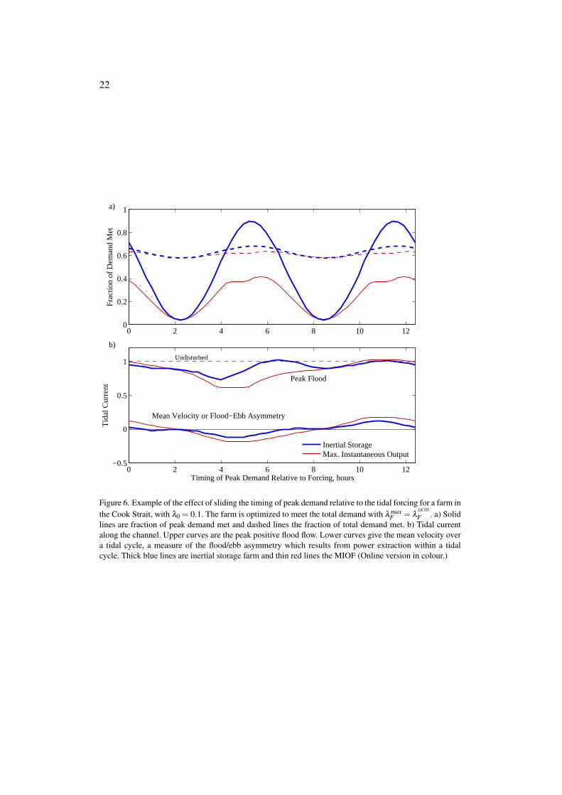
To understand the effect of sliding peak demand a periodic demand curve was movedrelative to the forcing through a full tidal cycle, simulating power production over a 14day period. The result is Fig. 6a which shows that while both MIOF and inertial storagefarms meet a similar fraction of the total demand, an inertial storage farm can meet up to90% of the peak demand, whereas a MIOF can meet less than 40% of the peak demand.Interestingly, for the inertial storage farm, the peak flood flow in Fig. 6b is generallystronger and its mean flow weaker than the MIOF. Thus the inertial storage farm isbetter able to mitigate any impacts of both flow speed reduction and tidal asymmetryresulting from power extraction to meet peak demand.

Fig. 7a shows the effect of bottom friction on the fraction of demand met, averagedover a 14 day period. For the Cook Strait example, the up to 90% of peak demand metby an inertial storage farm in Fig. 6a averages out as 58% over 14 days, meeting 30%more of the peak demand than a MIOF. Across the range of λ0, inertial stoage and MOIFfarms both meet a similar fraction of the total demand, with the average fraction of peakdemand met being significantly higher for inertial storage than MIOF farms for mediumto large channels, λ0 < 2.

Whereas the farms in Fig. 7a are optimized to meet total demand, those in Fig. 7bare optimized to meet peak demand. This figure demonstrates the flexibility of inertialstorage, which can trade meeting a reduced fraction of total demand for meeting a largerfraction of peak demand. This flexibility can even be exploited to a degree in smallchannels, with a relaxed threshold of λ0 < 3. The average current speed for both MIOFand inertial storage farms are similar when optimized to meet total demand, Fig. 7c,with both below the average speed in the undisturbed channel. For the farms optimizedto meet peak demand, average current speeds for the inertial storage farm are around10% higher than for the MIOF across the full range of channel sizes, Fig. 7d. This islikely a consequence of the inertial storage farm meeting less of the total demand andhence having a smaller time averaged farm drag coefficient.

5. Discussion

Inertial storage works by delaying power extraction until later in the half tidal cycle,allowing the forcing to further increase the flow speed. The stored energy’s lifetime islimited by dissipation due to bottom friction. If the farm is turned off and in the absenceof further forcing, (2.2) gives the velocity as u(t) = uint/(uintλ0ωt/uI +1), where uint isthe velocity at the time the farm turns off and uI is the velocity along the channel withno drag (which was used to non-dimensionalize u, §2 and (2.2)). Thus velocity in a farmwhich is turned off at peak flow would decay with a time scale, or storage time, of order

10

TD0 ≈uI

λ0ω |umax|. (5.1)

Table 1 shows that this frictional time scale for the example channels ranges between17 hours and 0.7 hours. The scale TD0 determines how beneficial delaying production is,because it indicates how long energy can persist within the flow before it is dissipatedby background bottom friction. Due to the non-linear drag law, turning the farm off ata lower initial velocity would give a longer time scale, i.e. increase storage times. ThusTD0 varies over the tidal cycle, with energy persisting longer for flows weaker than themaximum velocity. Consequently, TD0 indicates a lower limit for how long energy canpersist within the flow when the farm is turned off. For Cook Strait, this lower limit TD0=17 hours, which is much longer than the half tidal tidal cycle, thus delayed productioncan result in significantly higher total power production, Fig. 4a. For Pentland Firth, thelower limit is TD0=2.4 hours, less than half a tidal cycle, thus delayed production hasmore modest benefits.

In addition to switching off the farm, it could under produce by having λF < λ maxF ,

storing some energy for later in the cycle. Energy stored due to under production has ashorter storage time

TD ≈uI

(λ0 +λF(t ′))ω |umax|. (5.2)

Table 1 gives values of TD at peak flow based on a constant λF equal to the GC05 optimalvalue. The table shows that storage times for under production are longer than 1.7 hours,1.0 hours and 0.7 hours for the three examples.

Using inertial storage to exceed the GC05 limit relies on a combination of twoaspects of the physics. Firstly, using inertial storage to retain energy in the oscillatingflow, allows extraction to be delayed until as late as possible in the half tidal cycle.Secondly, it relies on the forcing continuing to accelerate the flow during the delay. Thiscontinued acceleration creates stronger flows, which generate more power because ofthe cubic dependance of power on velocity. As noted above, to effectively use inertialstorage to increase production the bottom friction time scale needs to be comparable to,or longer than, the half tidal cycle. This delays extraction as long as possible, taking fulladvantage of the acceleration due to forcing which continues throughout the half cycle.Thus it is no surprise that using inertial storage to increase production is only reallyeffective in large channels which have longer frictional time scales, with λ0 ≤ 1 in Fig.4a. What is surprising is that in both large and small channels a variable drag coefficientcan be used to maintain higher average flow speeds than those for a GC05 farm, Fig. 4b.Using the farm to maintain flow speeds closer to those in the undisturbed channel doesnot necessarily mean environmental effects are mitigated, but raises the possibility thatit may be possible to do so. Much more work on the effects of the change in strength ofthe flow over a full tidal cycle is needed in order to understand how to mitigate effects,such as those on sediment transport along the channel.

An inertial storage farm in Cook Strait can meet up to 90% of the example peakdemand curve, or 58% of peak demand when averaged over 14 days, even though thispeak demand is on top of a background demand equal to the channel’s GC05 potential.The ability to meet peaks in power demand is determined by the duration of the peakrelative to the frictional time scale. The example demand peaks have a width of 1.2hours, a duration comparable to the frictional time scale in the Pentland Firth, where on

11

average an inertial storage farm meets 15% more of peak demand than a MOIF. Usinginertial storage to delay peak production by 1-2 hours gives the farm the ability to betteralign with peak demand on more tidal cycles within a 14 day period, Fig. 7. Thus inertialstorage can be used over a much wider range of channel sizes to meet predictable peakdemand than the range for which it can be used to increase total power production.Consequently, tidal turbine farms in a wide range of channel sizes could have a role inproducing short bursts of power to meet predictable peaks in demand.

Another important time scale is the resonant period of the channel. Rapid changesin the farm’s drag coefficient may set up destructive seiching within the channel. Thefundamental seiche periods in the example channels are 85 min. 30 min. and 5 min.respectively, however a high drag coefficient farm may effectively halve the length ofthe channel, with seiches developing between the farm and the ends of the channelwith fundamental periods of half these values. Though channels are “short” for tidaloscillations, they are not short for these seiche periods, thus more work is needed tounderstand the dynamic effects of shallow water waves generated by rapid changes infarm drag coefficient. At the very least, any large change in the farm’s drag coefficientmust be made more gradually than the fundamental seiche period in order to minimizeany seiching within the channel.

The dynamical equation (2.2) used to solve for the velocity has an electricalanalogue. Inertia, which provides the storage here, is analogous to inductance and thedrag is equivalent to a non-linear resistor (Draper et al., 2014a). This electrical circuitanalogy could be used to understand how inertial storage could be exploited for arraysof tidal turbines within a network of interconnected channels, such as the Pentland Firth.

In the channel model of GC05, and that used here, it is assumed that the headlossbetween the ends of the channel is not affected by power extraction. Models for farms inthe open ocean have shown power extraction can have regional effects (Shapiro, 2011;Garrett and Cummins, 2013). Here, the channels are assumed to have a volumes smallcompared to the volume of the oceans they connect, thus any exchange of water betweenthe channel and the oceans will not significantly affect tidal patterns within the oceans. Arecent regional tidal model of the Pentland Firth has demonstrated that power extractionaffects the water level difference between the ends of the Firth by less than 10% (Draperet al., 2014b). Another effect of power extraction is to generate higher harmonics ofthe M2 tide through the non-linear effects of the quadratic drag law (2.2) (Adcock andDraper, 2014). This distortion of water level, both at the ends and within the channel, isnot part of the GC05 short channel model. However, its importance can be gauged fromtidal analysis of velocity solutions to (2.2). For the examples in Fig. 3 this nonlineareffect is small. Both the variable and constant λF farms create M4 tidal currents whichare only 5%-10% of the amplitude of the M2 constituent, slightly larger than the M4 of5% for the undisturbed velocity. While the model used here may not allow for the smalleffects of power extraction on water levels at the ends of the channel and non-lineardistortion of water levels, these effects are likely to be similar for farms with variableλF , constant λF and for MIOF farms. The advantages of variable λF farms presentedhere are given relative to these latter two types of reference farm, thus the relativeadvantages are unlikely to be sensitive to these effects. However, regional 2D depthaverage models which tackle the computationally challenging problem of optimizingthe farm drag coefficient in time must be developed to confirm this. These could exploitadjoint methods (Funke et al., 2014).

12

(a) Limitation of farm size and turbine efficiency

All the previous results assume that the farm is large enough to have a dragcoefficient as large as that required for a GC05 farm to realize the potential of the tidalchannel.

However economics or the available space within the channel may limit the size ofthe farm (Walters et al., 2013). Figure 4a demonstrated that halving the maximum dragcoefficient restricts the ability to use inertial storage to exceed the GC05 limit. Inertialstorage is likely be more useful in better meeting short duration peaks in demand as seenin Fig. 7. Figure 8 plots the fraction of total and peak demand met by inertial storagefarms with λ max

F ≤ λGC05

F in the example channels. In this figure both the inertial storagefarms and the MIOFs had λ max

F restricted to the fraction of λGC05

F given on the x-axis.To enable a fair comparison the demand was set in proportion to farm size. Backgrounddemand was set equal to that from a constant drag coefficient farm with the given λ max

Fand, as in previous examples, peak demand was set at three times background demand. InCook Strait, farms optimized to meet total demand can meet much more of peak demandthan MIOFs, while meeting a similar fraction of total demand, Figure 8a. Even a farmonly 1/5 the size of a GC05 farm still meets 10% more of peak demand than a MIOF.For the Firth the benefits when optimized to meet total demand are more modest, withinertial storage farms 1/2 the size of the GC05 farm meeting around 1% more of peakdemand, a figure which will be useful when seeking many small improvements frommature tidal turbine technology.

Farms optimized to meet peak demand, Fig. 8b, show significant benefits for inertialstorage farms across a wide range of farm sizes. In Cook Strait inertial storage farms 1/4the size of a GC05 farm can meet twice the fraction of peak demand met by a MIOF. Atλ max

F = 0.1λGC05

F a small inertial storage farm in the Strait still meets 12% more of peakdemand than a MIOF. The additional peak demand met results in a reduced fractionof total demand being met, demonstrating the ability to trade peak and total demandacross a wide range of farm sizes in the Strait. In the Firth an inertial storage farm has atleast a 10% advantage over a MIOF for farms larger than 1/5 the size of a GC05 farm.Even inertial storage farms in the shallow channel have more than a 10% advantage forfarms 1/2 the size of a GC05 farm. Thus, the malleability to trade meeting total demandwith meeting peak demand exists across a wide range of channel sizes and farm sizes.Much more work is required to estimate the number of turbines required to exploit thismalleability.

To exploit inertial storage, turbines will need to be built with the ability to rapidlychange their drag coefficient and power output. This would most likely be done byadjusting blade pitch or by varying the tip speed ratio. Existing tidal turbines alreadyuse changes in blade pitch to limit loads on the structure at flows above a rated velocity,or to rapidly stop production when marine mammals are nearby Douglas et al. (2008).The turbines in an inertial storage farm will likely need different design criteria, forexample rapidly turning turbines on and off several times per tidal cycle may increasethe risk of metal fatigue within the structure. This fatigue risk may also be compoundedby oscillating loads due to any seiching associated with rapid changes in drag coefficient.Another design consideration which will impact on both inertial storage and MIOF farmsis minimum operating flow speeds. A further consideration is the need for maximumoperating speeds to limit structural load. However, Fig. 5d suggests that loads on inertialstorage farms are similar to those on MIOFs.

13

To maintain navigation along the channel, tidal turbines will often only be permittedto fill part of a channel’s cross-section. The mixing of high speed flow which bypassesthe turbines, with slower flow passing through the turbines results in mixing losses(Garrett and Cummins, 2007). This mixing converts some of the flow’s energy in toheat (Corten, 2000). This energy loss, and that due to drag on any structures supportingthe turbines, reduces the energy available from the channel for electricity production(Vennell, 2012). The power lost to mixing and support structure drags are not accountedfor in the simple model given by (2.2) and (2.3). These losses will occur in both inertialstorage farms and MIOFs, thus more work is needed to determine how these lossesaffect the relative performance of these two farms. These losses would likely affect bothfarms to a similar degree, thus the relative benefits of inertial storage presented here maybe reasonable. An obvious next step is to extend the farm drag model to one built onactuator disk theory (Garrett and Cummins, 2007; Vennell, 2010). More work is alsorequired to understand the impacts of support structure drag, which may significantlyaffect the flow’s phase and magnitude, even if the turbines are not producing power.

6. Conclusions

This work shows that a variable farm drag coefficient can be used to make the timingof output from large tidal farms malleable. This malleability exploits the inertia of theoscillating tidal flow and can be used to produce more power, or better meet total or peakpower demand. This will give farm operators some flexibility about how they optimizethe farm’s output. For example, trading total power production off against meeting moreof the peak demand. They could also optimize the farm to minimize any environmentaleffects due to the flow speed reduction caused by power extraction.

For larger channels it is possible to exceed the GC05 limit on power production,while maintaining stronger currents. In some cases peak flows even exceed that in theundisturbed channel. This is possible, because more power can be produced in largerchannels by manipulating the phase of the currents relative to the forcing due to the headloss between the ends of the channel. Extracting more power is limited to medium tolarge channels, with λ0 < 1, Fig. 4a. However, the benefit of maintaining higher averageflow speeds over the half tidal cycle than those for a GC05 farm, extends across mostchannel sizes, Fig. 4b. Thus using inertial storage to maintain higher average speedsalong the channel, in order to minimize environmental impacts, may be more significantthan producing more power.

While producing more power is important, it is essential to generate power when itis required. Inertial storage can be used to delay production by 1-2 hours to better meetpredictable daily peaks in power demand in medium to large channels, with λ0 < 2, Fig.7a. Over a wider range of channel sizes, when λ0 < 3, inertial storage can be used totrade off meeting total demand against meeting more of the peak demand Fig. 7b, ormaintaining higher current speeds, Fig. 7d.

The example demand curve used here required the farm to attempt to meet abackground demand equal to the previous upper limit for production, GC05’s potential,plus an additional peak demand of twice the channel’s potential. This is a challengingdemand to meet. However, inertial storage can only be useful if the farm is large enoughto influence the flow’s amplitude and phase. Farms of this scale can meet up to 90% ofthis peak demand, depending on the timing of the demand relative to the phase of thetidal forcing in the channel, Fig. 6. How useful an inertial storage farm is depends on the

14

size of the channel and the size of the farm, Figs. 4, 7 and 8. In particular, inertial storageis useful in exceeding the GC05 limit for channels where the frictional time scale (5.2)is comparable to or longer than the half tidal cycle and useful in providing malleabilityto meet peaks in demand if the frictional time scale is comparable to or longer than theduration of those peaks.

This paper only presents the possibility that large tidal farms have some storagewhich could be used in a number of ways by farm operators. The simple 1D modelused here illustrates the mechanisms, but more sophisticated 2D and 3D models must bedeveloped in order to properly quantify the benefits. In addition, more work is needed todetermine how many turbines are required in a particular channel to make a farm largeenough to be able to develop a drag coefficient capable of manipulating the phase of thetidal currents. Clearly the farms must be large, though Fig. 8 demonstrates that inertialstorage farms much smaller than a GC05 farm have a significant ability to trade peakpower production for total power production. For large channels like Cook Strait thenumber of turbines required is of order 1,000 one MW turbines, 1/10 that required to fillits cross-section, Table 1. For medium sized channels like the Pentland Firth, the numberrequired could be around 300 one MW turbines, 1/5 that required to fill its cross-section.Thus, tidal turbine farms comparable in size to the largest wind farms may be able toexploit inertial storage. When tidal turbine technology matures even a 1% benefit fromexploiting inertial storage would be significant, as improvements of this size are alreadysignificant to large wind farms (Emspak, 2012). However, the turbines would need toform a “tidal fence”, spanning much of the channel’s width and have a high channelblockage ratio. Tidal turbine farms of this scale are well off in the future, but this workpresents ways large farms could be better utilized to meet varying energy demand whenthey are developed. Much further work is also needed to estimate the number of turbinesrequired and how best to arrange turbines within an inertial storage farm, along withwork to estimate the loads on the turbines in order to develop designs suitable for thesefarms.

Acknowledgments.

Craig Stevens, Tim Divett and Lara Wilcocks for their comments on drafts. Thiswork was supported by New Zealand Marsden Fund Grant number 12-UO-101.

References

Adcock, T. A. A., On the Garrett & Cummins limit, in Oxford Tidal Energy Workshop,2012.

Adcock, T. A. A., Unidirectional power extraction from a channel connecting a bay tothe open ocean, Proceedings of the Institute of Mechanical Engineers, Part A: Journalof Power and Energy, 227(8), 826–832, 2013.

Adcock, T. A. A., and S. Draper, Power extraction from tidal channels-multiple tidalconstituents, compound tides and overtides, Renewable Energy, 63, 797–806, doi:10.1098/rspa.2013.0072, 2014.

Adcock, T. A. A., S. Draper, G. T. Houlsby, A. G. L. Borthwick, and S. Serhadlıoglu,The available power from tidal stream turbines in the Pentland Firth, Proceedings of

15

the Royal Society A: Mathematical, Physical and Engineering Sciences, 469(2157),20130,072–20130,072, doi:10.1098/rspa.2013.0072, 2013.

Blunden, L. S., and A. S. Bahaj, Tidal energy resource assessment for tidal streamgenerators, Proc. of the Inst. MECH E Part A J. of Power and Energy, 221, 137–146(10), doi:10.1243/09576509JPE332, 2007.

Bryden, I., and S. Couch, ME1 Marine energy extraction: tidal resource analysis,Renewable Energy, 31(2), 133–139, 2006.

Corten, G., Heat generation by a wind turbine, in 14th IEA Symposium on theAerodynamics of Wind Turbines, vol. ECN report ECN-RX-01-001, p. 7, 2000.

Douglas, C., G. Harrison, and J. Chick, Life cycle assessment of the Seagen marinecurrent turbine, Proc. of the Inst. MECH E Part M J. of Eng. for the MaritimeEnvironment, 222(1), 1–12, doi:10.1243/14750902JEME94, 2008.

Draper, S., T. A. A. Adcock, A. G. Borthwick, and G. T. Houlsby, An electrical analogyfor the Pentland Firth tidal stream power resource, Proceedings Society of the RoyalSociety Part A, 470(2161), 20130,207, 2014a.

Draper, S., T. A. A. Adcock, A. G. Borthwick, and G. T. Houlsby, Estimate of theextractable Pentland Firth resource, Renewable Energy, 63, 650–657, 2014b.

Emspak, J., Dinosaur-inspired upgrades add bite to wind turbines, in New Scientist, vol.2882, 2012.

Funke, S. W., P. E. Farrell, and M. D. Piggott, Tidal turbine array optimisation usingthe adjoint approach, Renewable Energy, 63, 658–673, doi:10.1016/j.renene.2013.09.031, 2014.

Garrett, C., and P. Cummins, The power potential of tidal currents in channels, Proc.Royal Society A, 461, 2563–2572, 2005.

Garrett, C., and P. Cummins, The efficiency of a turbine in a tidal channel, Journal ofFluid Mechanics, 588, 243–251, 2007.

Garrett, C., and P. Cummins, Maximum power from a turbine farm in shallow water,Journal of Fluid Mechanics, 714, 634–643, doi:10.1017/jfm.2012.515, 2013.

Neill, S. P., E. J. Litt, S. J. Couch, and A. G. Davies, The impact of tidal stream turbineson large-scale sediment dynamics, Renewable Energy, 34(12), 2803 – 2812, doi:DOI: 10.1016/j.renene.2009.06.015, 2009.

Shapiro, G. I., Effect of tidal stream power generation on the region-wide circulation ina shallow sea, Ocean Science, 7(1), 165–174, doi:10.5194/os-7-165-2011, 2011.

Strang, G., Computational science and engineering, 290 pp., Wellesley-CambridgePress, 2007.

Vennell, R., ADCP measurements of tidal phase and amplitude in Cook Strait,New Zealand, Continental Shelf Research, 14, 353–364, doi:10.1016/0278-4343(94)90023-X, 1994.

16

Vennell, R., Observations of the Phase of Tidal Currents along a Strait, Journal ofPhysical Oceanography, 28(8), 1570–1577, doi:10.1175/1520-0485(1998)028<1570:OOTPOT>2.0.CO;2, 1998a.

Vennell, R., Oscillating barotropic currents along short channels, Journal ofPhysical Oceanography, 28(8), 1561–1569, doi:10.1175/1520-0485(1998)028<1561:OBCASC>2.0.CO;2, 1998b.

Vennell, R., Tuning turbines in a tidal channel, Journal of Fluid Mechanics, 663, 253–267, doi:10.1017/S0022112010003502, 2010.

Vennell, R., Estimating the power potential of tidal currents and the impact of powerextraction on flow speeds, Renewable Energy, 36, 3558–3565, doi:10.1016/j.renene.2011.05.011, 2011.

Vennell, R., The energetics of large tidal turbine arrays, Renewable Energy, 48, 210–219,doi:10.1016/j.renene.2012.04.018, 2012.

Vennell, R., Exceeding the Betz limit with tidal turbines, Renewable Energy, 55, 277–285, doi:10.1016/j.renene.2012.12.016, 2013.

Walters, R. A., M. R. Tarbotton, and C. E. Hiles, Estimation of tidal power potential,Renewable Energy, 51(25), 5e262, 2013.

17

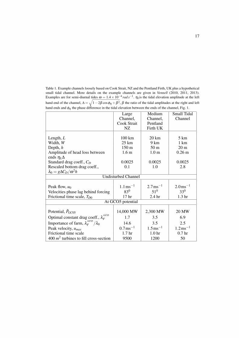
Table 1. Example channels loosely based on Cook Strait, NZ and the Pentland Firth, UK plus a hypotheticalsmall tidal channel. More details on the example channels are given in Vennell (2010, 2011, 2013).Examples are for semi-diurnal tides ω = 1.4× 10−4 rad s−1. ηLis the tidal elevation amplitude at the left

hand end of the channel, ∆ =√

1−2β cosφη +β 2, β the ratio of the tidal amplitudes at the right and lefthand ends and φη the phase difference in the tidal elevation between the ends of the channel, Fig. 1.

LargeChannel,

Cook StraitNZ

MediumChannel,PentlandFirth UK

Small TidalChannel

Length, L 100 km 20 km 5 kmWidth, W 25 km 9 km 1 kmDepth, h 150 m 50 m 20 mAmplitude of head loss betweenends ηL∆

1.6 m 1.0 m 0.26 m

Standard drag coeff., CD 0.0025 0.0025 0.0025Rescaled bottom drag coeff.,λ0 = g∆CD/ω2h

0.1 1.0 2.8

Undisturbed Channel

Peak flow, u0 1.1ms−1 2.7ms−1 2.0ms−1

Velocities phase lag behind forcing 830 510 330

Frictional time scale, TD0 17 hr 2.4 hr 1.3 hrAt GCO5 potential

Potential, PGC05 14,000 MW 2,300 MW 20 MWOptimal constant drag coeff., λ

GC05

F 1.7 3.5 6.9Importance of farm, λ

GC05

F /λ0 14.6 3.5 2.5Peak velocity, umax 0.7ms−1 1.5ms−1 1.2ms−1

Frictional time scale 1.7 hr 1.0 hr 0.7 hr400 m2 turbines to fill cross-section 9500 1200 50

18

Figure 1. Schematic of tidal channel connecting two large water bodies. The channel has length L and arectangular cross-section with width W and depth h. Flow, u(t) is forced along the channel by a differencein the relative amplitude of tidal water levels β in the two water bodies and/or a difference in the phase oftheir surface tides φη .

0 0.1 0.2 0.3 0.4 0.5 0.6−1

−0.5

0

0.5

1

1.5

2

No Farm λF= 0

Farm turns on

Turns off

Unlimited Variable λF

Farm turns on

Turns off

Limited Variable λF

Farm turns on

Turns off

Constant λF (GC05)

Farm turns on

Turns off

Pressure forcing

Tid

al C

urre

nt

Time in tidal cyles

Figure 2. Velocity solutions to (2.2) which maximize average power (2.3) for λ0 = 0. Red curve is theintuitively derived extreme case solution for λ max

F = ∞, blue curve is the optimal solution to (2.2) forλ max

F = λGC05

F and the green curve is GC05’s optimal solution for constant λF . Velocities are relative to thepeak flow in the channel when there is no farm.

19

0 0.1 0.2 0.3 0.4 0.5 0.60

0.2

0.4

0.6

0.8

1

1.2

Far

m D

rag

Coe

ff. λ F/λ

GC

05

a)

0 0.1 0.2 0.3 0.4 0.5 0.6−2

−1

0

1

2

Tid

al C

urre

nt

Peak Without Farm

b)

Constant λF , λ

0 = 0.1, Cook Strait

Variable λF , λ

0 = 0.1, Cook Strait

Constant λF , λ

0 = 1.0, Pentland Firth

Variable λF , λ

0 = 1.0, Pentland Firth

0 0.1 0.2 0.3 0.4 0.5 0.60

0.5

1

1.5

2

2.5

3

3.5

Pow

er

GC05 potential

c)

Time in tidal cycles

Figure 3. Limited variable drag coefficient and constant drag coefficient farms which maximize averagefarm output (2.3) in two of the example channels. Blue lines are for optimal variable drag coefficient withλ max

F = λGC05

F and green lines are for GC05’s optimal constant drag coefficient. Thick lines are for CookStrait and thin lines the Pentland Firth. a) Optimal variable farm drag coefficient λ

optF (t ′) relative to λ

GC05

Ffor each channel. b) Tidal current relative to the peak flow in the undisturbed channel. c) Instantaneouspower production of the farm relative to GC05’s potential for each channel, PGC05.

20

0 1 2 30.5

1

1.5

Background Bottom Friction, λ0

Pow

er R

el. t

o C

onst

ant λ

F

5% benefit

Cook StraitPentland Firth

Shallow Channel

a)

λmax

= λGC05

λmax

= 0.5 λGC05

0 1 2 30

0.5

1

1.5

Background Bottom Friction, λ0

Undisturbed

Max

. or

Ave

rage

Spe

ed

GC05

Cook StraitPentland Firth

Shallow Channel

b)

Figure 4. The effect of increasing bottom friction on power production by farm with optimal variable dragcoefficient. Labels show λ0 for the three example channels. a) Average power relative to a constant dragcoefficient farm with given λ max

F b) Velocities relative to the velocity in channel with no farm at given λ0.Solid lines show peak flow and the dashed lines the flow speed averaged over a tidal cycle. (Online versionin colour.)

21

0 2 4 6 8 10 120

1

2

3

Pow

er Optimized for Total Demand

a)

Power DemandInertial StorageMax. Instantaneous OutputGC05

0 2 4 6 8 10 120

0.2

0.4

0.6

0.8

1λ

GC05

Far

m D

rag

Coe

ffici

entb)

0 2 4 6 8 10 12

−1

−0.5

0

0.5

1Undisturbed Maximum

Vel

ocity

c)

0 2 4 6 8 10 12−1

−0.5

0

0.5

1 Maximum Force on GC05 Farm

For

ce o

n F

arm

Time within tidal cycle, Hours

d)

Figure 5. Example of a farm in the Cook Strait example channel optimized to meet the total demand (4.1)given by the gray curve with λ max

F = λGC05

F . The peak in the Gaussian demand curve is at 5.5 hours. a)Power and demand relative to PGC05. An inertial storage farm meets 68% of total demand and 90% of peakdemand, whereas a MIOF meets 63% of total demand but only 40% of peak demand. b) Optimized variablefarm drag coefficient relative to λ

GC05

F . c) Velocity along the channel relative to velocity when there is nofarm. d) Total force on the farms relative to the maximum force on a GC05 farm.

22

0 2 4 6 8 10 120

0.2

0.4

0.6

0.8

1

Fra

ctio

n of

Dem

and

Met

a)

0 2 4 6 8 10 12−0.5

0

0.5

1

Timing of Peak Demand Relative to Forcing, hours

Tid

al C

urre

nt

Undisturbed

Peak Flood

Mean Velocity or Flood−Ebb Asymmetry

b)

Inertial StorageMax. Instantaneous Output

Figure 6. Example of the effect of sliding the timing of peak demand relative to the tidal forcing for a farm inthe Cook Strait, with λ0 = 0.1. The farm is optimized to meet the total demand with λ max

F = λGC05

F . a) Solidlines are fraction of peak demand met and dashed lines the fraction of total demand met. b) Tidal currentalong the channel. Upper curves are the peak positive flood flow. Lower curves give the mean velocity overa tidal cycle, a measure of the flood/ebb asymmetry which results from power extraction within a tidalcycle. Thick blue lines are inertial storage farm and thin red lines the MIOF (Online version in colour.)

23

0

0.2

0.4

0.6

0.8Optimized for Total Demand

Ave

r. D

eman

d Fr

actio

n M

et

Cook StraitPentland Firth

Shallow Channel

a)

0

0.2

0.4

0.6

0.8Optimized for Peak Demand

Ave

r. D

eman

d Fa

ctio

n M

eet

Cook StraitPentland Firth

Shallow Channel

b)

0 0.5 1 1.5 2 2.50

0.2

0.4

0.6

0.8

1

Bottom Friction, λ0

Ave

arge

Cur

rent

Spe

ed

Optimized for Total Demand

Cook StraitPentland Firth

Shallow Channel

c)

Inertial StorageMax. Instantaneous Output

0 0.5 1 1.5 2 2.50

0.2

0.4

0.6

0.8

1Optimized for Peak Demand

Ave

arge

Cur

rent

Spe

ed

Bottom Friction, λ0

Cook StraitPentland Firth

Shallow Channel

d)

Figure 7. Fraction of demand met averaged over 14 days for inertial storage farms and MIOF farms in arange of channel sizes with λ max

F = λGC05

F . Dashed lines give fraction of total demand met, solid lines thefraction of peak demand met. a) Farms optimized to meet total demand (4.1). b) Farms optimized to meetpeak demand (4.2) are able to trade meeting more peak demand for meeting less of the total demand. c+d)Average current speed, relative to average current speed in the undisturbed channel, for farms optimizedto meet total demand and peak demand respectively. Thick blue lines are inertial storage farm and thin redlines the MIOF (Online version in colour.)

24

0 0.2 0.4 0.6 0.8 10.5

1

1.5

2

2.5

λFmax / λ

GC05

Rel

. fra

ctio

n of

dem

and

met

Optimized for Total Demand

a)

Cook StraitPentland FirthShallow Channel10% advantage

0 0.2 0.4 0.6 0.8 10.5

1

1.5

2

2.5Optimized for Peak Demand

Rel

. fra

ctio

n of

dem

and

met

λFmax / λ

GC05

b)

Figure 8. Effect of varying λ maxF on the fraction of demand met by an inertial storage farm averaged over 14

days relative to a MIOF in the three example channels. Solid lines are ratio of the fraction of peak demandmet by an inertial storage farm to the fraction met by a MIOF with the same λ max

F . Dashed lines give theratio for the fractions of total demand met. Horizontal dotted line indicates ratio giving an inertial storagefarm a 10% advantage of over a MIOF. a) Farms optimized to meet total demand (4.1). b) Farms optimizedto meet peak demand (4.2). (Online version in colour.)